Bifurcations in the Herd Immunity Threshold for Discrete-Time Models of Epidemic Spread
Abstract
We performed a thorough sensitivity analysis of the herd immunity threshold for discrete-time SIR compartmental models with a static network structure. We find unexpectedly that these models violate classical intuition which holds that the herd immunity threshold should monotonically increase with the transmission parameter. We find the existence of bifurcations in the herd immunity threshold in the high transmission probability regime. The extent of these bifurcations is modulated by the graph heterogeneity, the recovery parameter, and the network size. In the limit of large, well-mixed networks, the behavior approaches that of difference equation models, suggesting this behavior is a universal feature of all discrete-time SIR models. These results suggest careful attention is needed in both selecting the assumptions on how to model time and heterogeneity in epidemiological models and the subsequent conclusions that can be drawn.
Introduction
The herd immunity threshold (henceforth, HIT) is a key epidemiological quantity that signifies the end of the growth phase of an epidemic. During the COVID-19 pandemic, the HIT has both received a great deal of attention from scientists, media, and the public, as well has been a significant source of contention amongst policymakers [13, 26, 21]. Despite its importance, the behavior of this quantity beyond classical epidemiological models is still not well understood. How the HIT is affected by heterogeneity in the spacing of infections in time and heterogeneity in contact structure remain open areas of research.
In constructing epidemic models, a key conceptual decision is deciding on how to represent the flow of time, which can be done in either a continuous or discrete fashion. For continuous-time models of epidemic spread, the underlying premise is that contact events or potential infection events are well-mixed and evenly distributed through time. Typically, this assumption is formalized as contact events being a Poisson-distributed transmission process. This is a common and convenient assumption which is used both in classical differential equation-based models, as well as in graph network models [29, 28, 7]. The assumption is also more amenable to mathematical analysis techniques.
In contrast, there are arguments that have been posed in the literature on the utility of a model of infections that is fundamentally discrete-time [9, 3, 14, 2]. Firstly, since case data (both prevalence and incidence) are typically reported discretely on a daily or weekly basis [5], it is worth investigating the consequences of models that update time on the same time-scale as the real-world data. Secondly, human mobility patterns have been empirically shown to be quite regular and concentrated in time [8, 27], suggesting that social contact peaks at certain times during the day. These bursts of social activity are opportunities for infection that are more concentrated than a Poisson process would suggest. Finally, from a computational standpoint, it is sometimes necessary and easier to deal with discrete-time models.
It is an open question whether these two representations of time significantly differ in their behavior and predictions for key epidemic quantities, such as the HIT. While we do not believe time to actually be discrete in reality, there are valid reasons a modeller may choose either type of time dynamic. Thus we explore the understudied assumption of modeling time as discrete and the resulting implications of that assumption as it relates to the HIT. Any resulting differences in the behavior of the HIT must be taken as a consequence of the modeling of time, rather than necessarily a reflection of physical reality. As will be shown, a seemingly innocuous choice on how to represent time can have rather dramatic downstream consequences, serving as an important reminder to all modelers to consider their basis of assumptions meticulously.
Another key choice in modeling epidemics is establishing the structure for how infections will spread. Realistic models of disease spread are critical for accurate forecasting and management of epidemics, as the COVID-19 pandemic has made clear. Classical models of disease spread, which have been very useful for general understanding of epidemic phenomena and for their analytical tractability in certain cases, can make unrealistic modelling assumptions about the structure of the underlying contact network. This simplification can render these models unsatisfactory as tools for predicting the extent and severity of disease spread. For instance, the classical SIR compartmental model assumes a contact network structure wherein each individual is (1) connected to all other individuals in the network and (2) the size of the network approaches a magnitude that allows for stochastic effects of spread to be ignored. Often, neither of these assumptions is realistic. One consequence is that these assumptions do not mathematically allow for known epidemic phenomena, such as superspreaders [19, 6, 22], to occur. Recently, the explosion of computational resources for simulation and availability of granular data for contact network estimation have made agent-based models that simulate spread of epidemics on realistic networks a viable and practical tool [10, 25]. Recent work has also begun to explore the impact of heterogeneity on HIT [12, 4, 16, 11, 20].
To investigate how these modeling choices influence the HIT, we considered simulations of agent-based models that use graphs of varying degree heterogeneity with infection events occurring in discrete time. As a result, the states of all individuals in the network are updated simultaneously at each time-step. This relaxes the above assumption that infections occur uniformly through continuous time. It is the purpose of this paper to shed light on the highly non-classical behaviors these models can generate and subsequently discuss the implications for epidemic forecasting.
Results
Results are reported for the following numerical experiments. We conducted simulations of SIR epidemic spread on an agent-based model, where individuals infect contacts on a network structure represented by a graph. We performed a thorough sensitivity analysis on four critical model parameters: the network heterogeneity parameter , which controls the heterogeneity in the degree-distribution of the network generated [23]; the transmission probability , which determines how likely an infected individual is to infect a susceptible neighbor in a given time-step; the spontaneous recovery parameter , which controls how probable it is that an infected individual recovers in a given time-step, and the size of the network .
Our simulations generate time-series of the number of individuals in a given compartment: Susceptible, Infected, or Recovered, from which we compute key epidemic statistics: the HIT and the time at the peak of infection prevalence. For ODE-based SIR models, the HIT can be derived analytically in terms of the basic reproduction number [1]. Since does not have a standard analogue in the context of epidemic spread on a network, we have defined the HIT based on a key feature on when it would classically occur, namely that the HIT occurs at the peak of infection prevalence. Here we defined HIT as the cumulative proportion of the population that has been reached by the disease by the time the infection prevalence peaks. This definition is meant to intuitively align with classical expectations of a herd immunity threshold, namely that it is the point at which the effective reproductive number equals 1 and where the epidemic is no longer growing in size.
As we scan through parameter space, we study the distribution and behavior of the HIT and time to infection prevalence to understand the behavior of epidemic peaks under iteration. Although we allow the topology of the contact networks to vary, all edges carry equal weight . For each unique quadruplet of parameters: transmission probability, recovery probability, graph heterogeneity, and size given as , we run 150 simulations, randomly infecting a small initial fraction of nodes on the graph. Further details of the construction of the contact network and the model for simulations can be found in the Methods section.
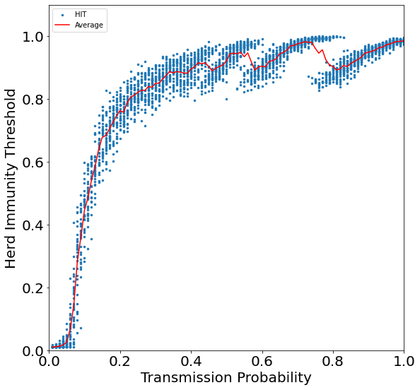
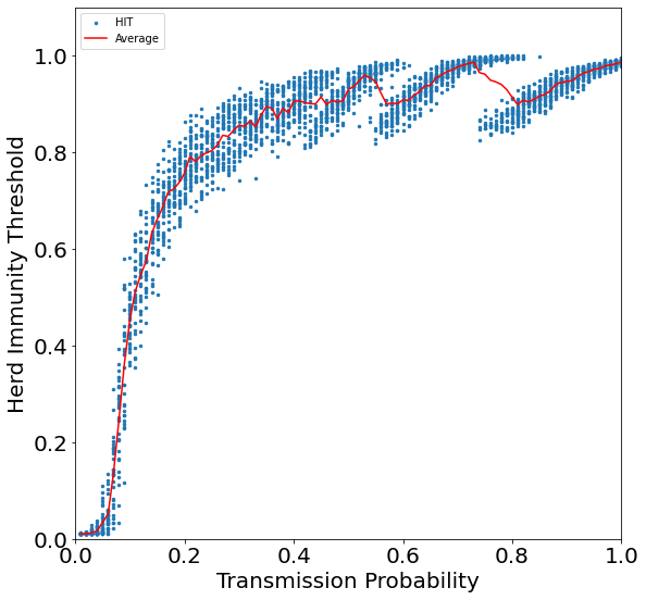
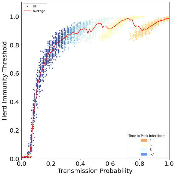
In Figure 1, we display the HIT as a function of transmission probability for a single triple and the full range of transmission probabilities (). Each point represents the results of a single simulated epidemic, and the red line represents the empirical average across iterations for a single value of .
Starting from the lowest transmission probability and moving right, we first encounter a subcritical phase gated by a critical threshold value of . Upon crossing the threshold, the average HIT rapidly grows before saturating at an asymptotic phase which is characterized by oscillations in the average HIT and bifurcations in the individual point clouds. In what follows, we present further results that test the sensitivity of this bifurcation behavior to various parameters of the SIR model.
Increased Contact Heterogeneity Suppresses Bifurcations
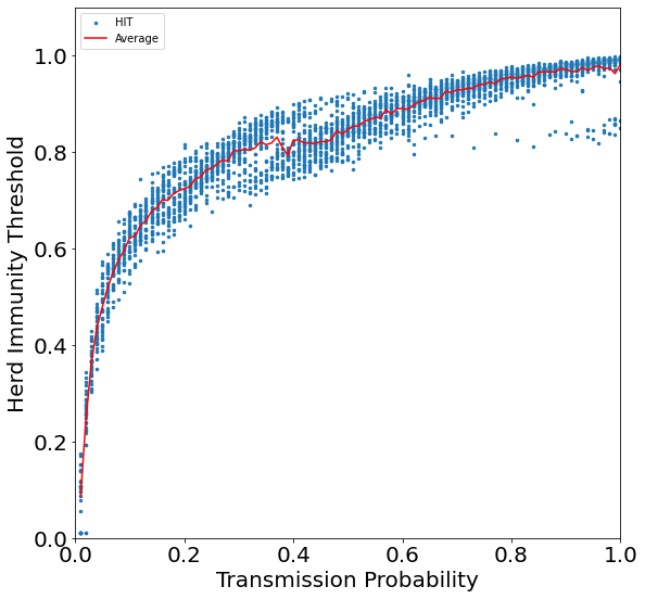
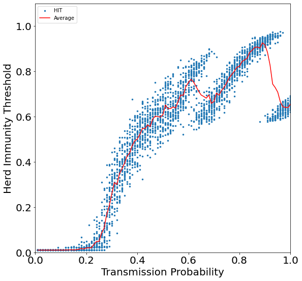
We investigated the sensitivity of the HIT to the heterogeneity of the underlying contact network. The heterogeneity of the network is given by a single parameter which, at , specifies a set of graphs with completely homogeneous degree distributions (all nodes in the graph have the same degree), while specifies a graph whose degree distribution is heavy-tailed. More details on this parameter and the method used to generate the degree distributions is included in the Methods section.
In Figure 2, it can be seen that the HIT is generally increasing as a function of the transmission probability. More homogeneous graphs have a subcritical regime where the HIT and epidemic does not grow to an appreciable size until a critical transmission probability threshold is reached. The disappearance of this threshold in more heterogeneous networks, particularly scale-free networks, is well documented [24]. Increasing graph heterogeneity appears to decrease the number and the gaps in the bifurcations in the distribution of the HIT.
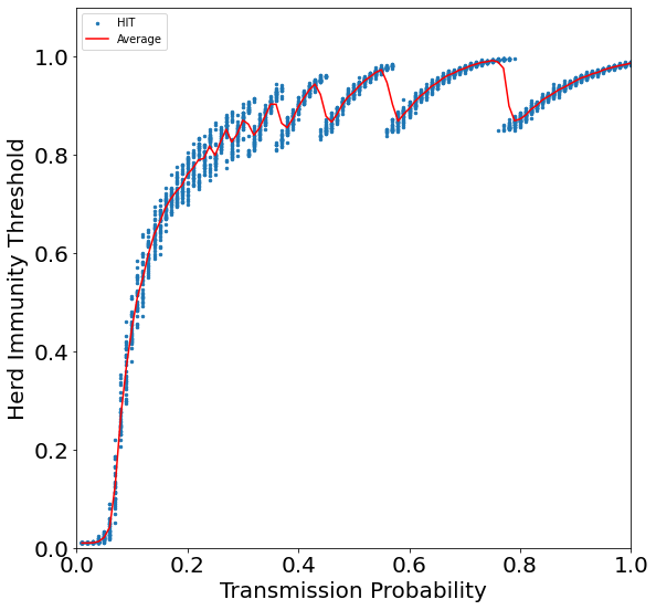
Increased Recovery Probability Drives Variability in Epidemic Peak
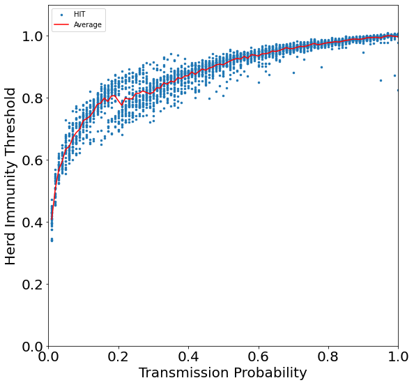
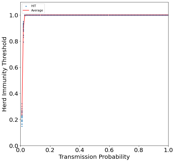
We investigated the sensitivity of the HIT to the spontaneous recovery probability . In Figure 3, it can be seen that as (which is the SI limit of the SIR model) there is no bifurcation in the HIT observed and convergence to a completely infected network () is very rapid, as there is no recovery. As we increase the recovery probability, the convergence to the asymptotic phase is slower as a function of transmission probability. In addition, the extent of the subcritical phase becomes elongated for higher recovery probabilities. The range of potential HIT values also increases with increasing recovery probability, allowing for significantly lower HIT values to be possible. Increasing the recovery probability also increases the magnitude of the gaps in HIT bifurcations in the asymptotic phase.
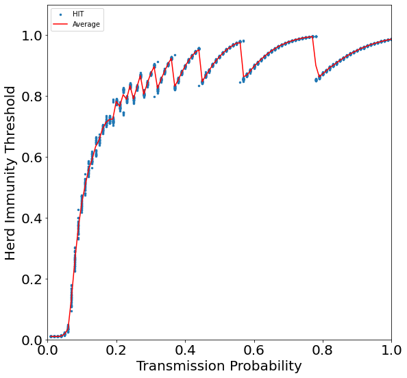
Bifurcations Sharpen and Increase in Number with System Size
We considered the effect of changing the size of the system on the HIT by changing the number of nodes on which we simulate the epidemic. In Figure 4, increasing the order of magnitude of the nodes leads to a greater number and frequency of bifurcations in the HIT. Additionally, the variance around the average HIT value for a given transmission probability decreases as the size of the graph increases.
Discussion
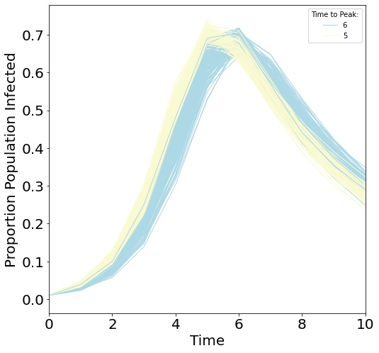
The most notable of the non-classical behaviors presented is the bifurcation gaps of the HIT, as seen in Figures 1-4. The classical intuition that as the transmission parameter increases, the HIT will also monotonically increase is clearly violated both at the level of individual simulations (blue dots), as well as for averages over simulations runs (red line). In certain parameter regimes, for instance Figure 3c, the difference in HIT values across the bifurcation gap can be substantial: for a , the epidemic may realize an HIT of 0.6 or 1 depending on how the stochastics of the epidemic process play out. We thus observed that even the simplest models of discrete-time disease spread on networks produces behavior that is highly non-classical and even counter-intuitive by the standard results of ODE-based SIR models in the literature.
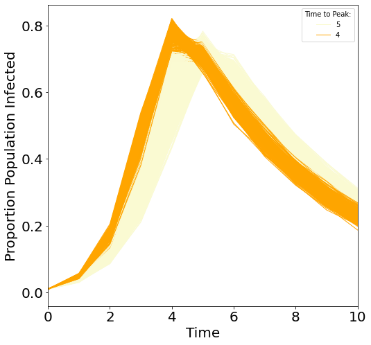
The origin of this bifurcation behavior can be unraveled by inspecting the infection curves of the individual simulation runs as a function of time. To demonstrate, let us look at the distribution of infection curves for the interval of in Figure 1, which includes a single bifurcation. We see that when we plot the infection curves for simulations with parameter values of in this interval as a function of time (Figure 5a), all of the simulation runs segregate into exactly two groups: runs that peak at time 5 (yellow curves) and time 6 (blue curves) respectively. We note that both groups of infection curves are similar in shape, which can be verified by calculating a convolution of curves representative of the two groups, reflecting that both groups are drawn under the same parameter values. Importantly however, we note that all of the curves in yellow grow at a rate faster than the blue curves during the growth phase (times 1-4). In addition, the individual runs in the yellow group recover at a slightly faster rates, as seen by an earlier decline in infections compared to blue curves. Thus, small absolute differences in the initial spreading dynamics due to stochasticity differentiates runs into two groups, allowing some runs to peak one time-step earlier without shifting the bulk of the infection curve. While the infection curves between the two groups overlap heavily, importantly, the position of the peak shifts from one shoulder to another. Since the HIT is a cumulative summation that is sensitive to where the peak occurs, even a difference of a single time step can cause a large difference in the HIT attained between runs. Increasing the transmission probability amounts to shifting the infection curves to larger values of time, while still maintaining this dimorphism between faster-peaking runs and slower-peaking runs, as seen in Figures 5b,c.
The explanation above is also consistent with the trends observed in how these bifurcations are dependent on the other parameters of the model. For instance, as the graph becomes more heterogeneous () the bifurcations decrease in frequency. As heterogeneity increases, the networks become more heavy-tailed in the degree distribution. This causes the average path length between pairs of nodes to decrease as shortcuts can be taken through hubs. This is in contrast with homogeneous networks, which are characterized by a lattice-like structure and feature much longer minimum path lengths between any two nodes in the network. In effect, heterogeneity in the network allows a larger set of initial conditions and transmission probabilities to lead to a full blown epidemic. For example, in Figure 2c the time to the peak of infection prevalence peaks quickly. This fast time to peak is the same for all runs in the entire range of after the first bifurcation. There are no further bifurcations because the network can not peak any faster since the average shortest path length sets a topological lower bound on the time to peak of infections.
The impact of the recovery rate on the phenomena can also be disentangled. In the SI limit () the bifurcation behavior does not manifest, whereas in the limit of immediate recovery in the time-step following infection () the bifurcation jumps are the most dramatic. Intuitively, the increased recovery parameter makes it more difficult for the epidemic to continue spreading, which allows for both lower HIT values and for critical transmission probability threshold needed for a non-trivial epidemic. Increased recovery also makes the epidemic trajectory more dependent on the initial conditions, which is reflected on the wider variation in HIT values for a given . The effect of system size agrees with intuition that as the system size increases one should expect stochastic effects to decrease in relative magnitude. This is reflected by the decrease in smearing of data points around the average HIT with increasing system size. This is sensible, as deterministic systems should only attain a single HIT value for a given set of parameter values, given they always generate a single epidemic path.
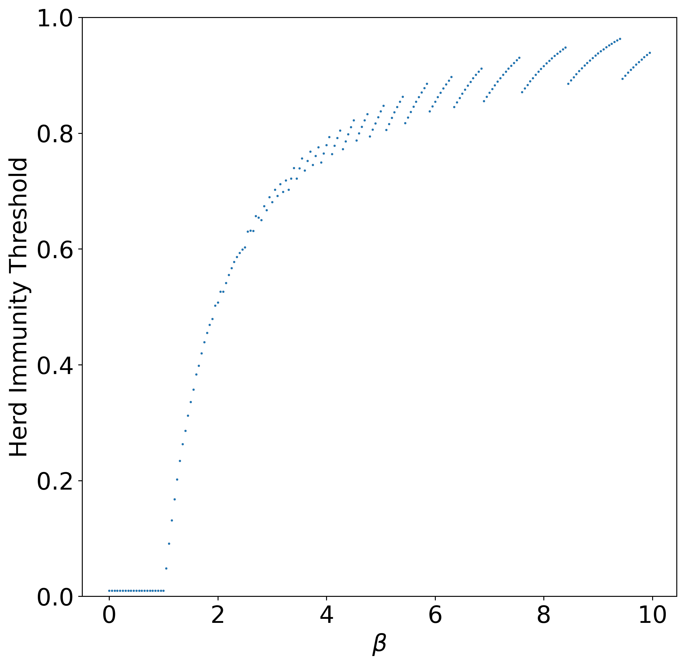
With the intuition given by the sensitivity analysis, we might expect then that in the large, well-mixed limit, the behavior of the HIT for network models should approach that of the Kermack-McKendrick SIR model [17]. Indeed, we found that the network behavior recapitulates the same qualitative behavior as the deterministic SIR equations under time discretization (Figure 6). Equations for the SIR model in the form of difference equations can be found in the Methods. This implies the bifurcation behavior of the HIT at high transmission probabilities is not restricted to SIR models that contain either network structure or stochasticity. This suggests that these bifurcations and oscillations in HIT may exist in certain regions of parameter space for all discrete-time SIR models. Other discrete-time SIR models are reported in the literature [9, 18].
Conclusion
In general, increasing the transmission probability causes the epidemic to spread more rapidly in the population, which decreases the time to peak of infections. However, for discrete-time models this is necessarily a transition from one discrete time-step to another. The incremental nature of discrete time directly yields the observed bifurcation behavior in the HIT. That the observed bifurcation behavior occurs rather generically in discrete-time SIR models suggests that a modeler is faced with a key decision when deciding on how to represent time conceptually in their models. For the reasons mentioned previously, both continuous- and discrete-time models present distinct advantages that merit their use. Here we have illustrated some key behaviors and even unintended impacts that may arise when making the choice to model time discretely and considering the role of heterogeneity. This may prove insightful not only to epidemic modelers, but also those in position to make public policy who need to understand the limits of the conclusions they can draw from the models being employed [15]. That such a simple alteration to the SIR model can lead to highly non-classical behavior suggests it would be prudent for the epidemiological community to carefully revisit and to inspect even the most basic assumptions being used in models.
References
- [1] Roy M. Anderson and Robert M. May “Vaccination and herd immunity to infectious diseases” Number: 6044 Publisher: Nature Publishing Group In Nature 318.6044, 1985, pp. 323–329 DOI: 10.1038/318323a0
- [2] Per Block et al. “Social network-based distancing strategies to flatten the COVID-19 curve in a post-lockdown world” Number: 6 Publisher: Nature Publishing Group In Nature Human Behaviour 4.6, 2020, pp. 588–596 DOI: 10.1038/s41562-020-0898-6
- [3] Fred Brauer, Zhilan Feng and Carlos Castillo-Chávez “Discrete epidemic models” Company: Mathematical Biosciences & Engineering Distributor: Mathematical Biosciences & Engineering Institution: Mathematical Biosciences & Engineering Label: Mathematical Biosciences & Engineering Publisher: American Institute of Mathematical Sciences In Mathematical Biosciences & Engineering 7.1, 2010, pp. 1 DOI: 10.3934/mbe.2010.7.1
- [4] Tom Britton, Frank Ball and Pieter Trapman “A mathematical model reveals the influence of population heterogeneity on herd immunity to SARS-CoV-2” Publisher: American Association for the Advancement of Science In Science 369.6505, 2020, pp. 846–849 DOI: 10.1126/science.abc6810
- [5] CDC “COVID Data Tracker”, 2020 URL: https://covid.cdc.gov/covid-data-tracker
- [6] Serina Chang et al. “Mobility network models of COVID-19 explain inequities and inform reopening” Number: 7840 Publisher: Nature Publishing Group In Nature 589.7840, 2021, pp. 82–87 DOI: 10.1038/s41586-020-2923-3
- [7] Zesheng Chen “Discrete-Time vs. Continuous-Time Epidemic Models in Networks” Conference Name: IEEE Access In IEEE Access 7, 2019, pp. 127669–127677 DOI: 10.1109/ACCESS.2019.2940132
- [8] Eunjoon Cho, Seth A. Myers and Jure Leskovec “Friendship and mobility: user movement in location-based social networks” In Proceedings of the 17th ACM SIGKDD international conference on Knowledge discovery and data mining, KDD ’11 New York, NY, USA: Association for Computing Machinery, 2011, pp. 1082–1090 DOI: 10.1145/2020408.2020579
- [9] Odo Diekmann, Hans G. Othmer, Robert Planqué and Martin C.. Bootsma “The discrete-time Kermack–McKendrick model: A versatile and computationally attractive framework for modeling epidemics” Publisher: Proceedings of the National Academy of Sciences In Proceedings of the National Academy of Sciences 118.39, 2021, pp. e2106332118 DOI: 10.1073/pnas.2106332118
- [10] Stephen Eubank et al. “Modelling disease outbreaks in realistic urban social networks” Number: 6988 Publisher: Nature Publishing Group In Nature 429.6988, 2004, pp. 180–184 DOI: 10.1038/nature02541
- [11] Matthew J Ferrari, Shweta Bansal, Lauren A Meyers and Ottar N Bjørnstad “Network frailty and the geometry of herd immunity” Publisher: Royal Society In Proceedings of the Royal Society B: Biological Sciences 273.1602, 2006, pp. 2743–2748 DOI: 10.1098/rspb.2006.3636
- [12] Paul Fine, Ken Eames and David L. Heymann ““Herd Immunity”: A Rough Guide” In Clinical Infectious Diseases 52.7, 2011, pp. 911–916 DOI: 10.1093/cid/cir007
- [13] Arnaud Fontanet and Simon Cauchemez “COVID-19 herd immunity: where are we?” Number: 10 Publisher: Nature Publishing Group In Nature Reviews Immunology 20.10, 2020, pp. 583–584 DOI: 10.1038/s41577-020-00451-5
- [14] Nancy Hernandez-Ceron, Zhilan Feng and Carlos Castillo-Chavez “Discrete epidemic models with arbitrary stage distributions and applications to disease control” In Bulletin of mathematical biology 75.10, 2013, pp. 1716–1746 DOI: 10.1007/s11538-013-9866-x
- [15] Lyndon P. James, Joshua A. Salomon, Caroline O. Buckee and Nicolas A. Menzies “The Use and Misuse of Mathematical Modeling for Infectious Disease Policymaking: Lessons for the COVID-19 Pandemic” Publisher: SAGE Publications Inc STM In Medical Decision Making 41.4, 2021, pp. 379–385 DOI: 10.1177/0272989X21990391
- [16] Matt J Keeling and Ken T.D Eames “Networks and epidemic models” Publisher: Royal Society In Journal of The Royal Society Interface 2.4, 2005, pp. 295–307 DOI: 10.1098/rsif.2005.0051
- [17] William Ogilvy Kermack, A.. McKendrick and Gilbert Thomas Walker “A contribution to the mathematical theory of epidemics” Publisher: Royal Society In Proceedings of the Royal Society of London. Series A, Containing Papers of a Mathematical and Physical Character 115.772, 1927, pp. 700–721 DOI: 10.1098/rspa.1927.0118
- [18] Matthias Kreck and Erhard Scholz “Back to the Roots: A Discrete Kermack–McKendrick Model Adapted to Covid-19” In Bulletin of Mathematical Biology 84.4, 2022, pp. 44 DOI: 10.1007/s11538-022-00994-9
- [19] J.. Lloyd-Smith, S.. Schreiber, P.. Kopp and W.. Getz “Superspreading and the effect of individual variation on disease emergence” Number: 7066 Publisher: Nature Publishing Group In Nature 438.7066, 2005, pp. 355–359 DOI: 10.1038/nature04153
- [20] C… Metcalf, M. Ferrari, A.. Graham and B.. Grenfell “Understanding Herd Immunity” In Trends in Immunology 36.12, 2015, pp. 753–755 DOI: 10.1016/j.it.2015.10.004
- [21] David M Morens, Gregory K Folkers and Anthony S Fauci “The Concept of Classical Herd Immunity May Not Apply to COVID-19” In The Journal of infectious diseases 226.2, 2022, pp. 195–198 DOI: 10.1093/infdis/jiac109
- [22] Bjarke Frost Nielsen, Lone Simonsen and Kim Sneppen “COVID-19 Superspreading Suggests Mitigation by Social Network Modulation” Publisher: American Physical Society In Physical Review Letters 126.11, 2021, pp. 118301 DOI: 10.1103/PhysRevLett.126.118301
- [23] Sinan A. Ozbay and Maximilian M. Nguyen “Parameterizing Network Graph Heterogeneity using a Modified Weibull Distribution” arXiv, 2022 DOI: 10.48550/arXiv.2212.06994
- [24] Romualdo Pastor-Satorras and Alessandro Vespignani “Epidemic Spreading in Scale-Free Networks” Publisher: American Physical Society In Physical Review Letters 86.14, 2001, pp. 3200–3203 DOI: 10.1103/PhysRevLett.86.3200
- [25] Romualdo Pastor-Satorras, Claudio Castellano, Piet Van Mieghem and Alessandro Vespignani “Epidemic processes in complex networks” Publisher: American Physical Society In Reviews of Modern Physics 87.3, 2015, pp. 925–979 DOI: 10.1103/RevModPhys.87.925
- [26] Haley E. Randolph and Luis B. Barreiro “Herd Immunity: Understanding COVID-19” In Immunity 52.5, 2020, pp. 737–741 DOI: 10.1016/j.immuni.2020.04.012
- [27] Chaoming Song, Zehui Qu, Nicholas Blumm and Albert-László Barabási “Limits of Predictability in Human Mobility” Publisher: American Association for the Advancement of Science In Science 327.5968, 2010, pp. 1018–1021 DOI: 10.1126/science.1177170
- [28] Eugenio Valdano, Michele Re Fiorentin, Chiara Poletto and Vittoria Colizza “Epidemic Threshold in Continuous-Time Evolving Networks” Publisher: American Physical Society In Physical Review Letters 120.6, 2018, pp. 068302 DOI: 10.1103/PhysRevLett.120.068302
- [29] Piet Van Mieghem, Jasmina Omic and Robert Kooij “Virus Spread in Networks” Conference Name: IEEE/ACM Transactions on Networking In IEEE/ACM Transactions on Networking 17.1, 2009, pp. 1–14 DOI: 10.1109/TNET.2008.925623
Methods
Construction of Contact Networks With A Specified Amount of Heterogeneity
We generate the graph as follows. First, we select a value of , with representing a highly homogeneous degree distribution and representing a highly heterogeneous degree distribution. The value of chosen maps to a unique value of where is the shape parameter of the Weibull distribution, through the transformation
Next, we fix , which can be thought of as the number at which the degree distribution will be centered at. Simulations in the Results section are conducted on graphs of 1000 nodes and 5000 connections. Simulations on graphs several orders of magnitude larger produce results that are similar.
The scale parameter and shape parameter specify a unique 2-parameter Weibull distribution, given by:
| (1) |
We then sample from this distribution to achieve the desired network size. With the sample obtained, we construct the graph using the configuration model. This specifies a graph which is sampled from the space of all graphs that are compatible with the degree distribution generated per the above procedure.
Simulation of a Discrete-Time SIR Model on A Graph
The model of the simulation is as follows. Given a graph representing the contact network of interest, fix a transmission probability and recovery probability :
-
1.
At time , fix a small fraction of nodes to be chosen uniformly on the graph and assign them to the Infected state. The remaining fraction of nodes start as Susceptible.
-
2.
For each , for each pair of adjacent S and I nodes, the susceptible node becomes infected with probability .
-
3.
For each , each infected node recovers with probability .
-
4.
At time , record two quantities: The final attack rate and the herd immunity threshold at the peak of the epidemic.
-
5.
Repeat steps (1-4) n = 150 times for each value of .
-
6.
Repeat steps (1-5) for each value of .
Discretizing the SIR Ordinary Differential Equations Model
To numerically compute the trajectory of the deterministic system of ODEs, we discretize the Kermack-McKendrick SIR model and then apply Euler’s method. The SIR equations are given as:
| (2) | ||||
| (3) | ||||
| (4) |
Commonly, the Euler method is used when numerically integrating these equations. For an ordinary differential equation of the form this amounts to computing an approximate solution according to
| (5) |
In the case of the SIR model we can write:
| (6) |
and similarly for and , where tilde denotes an approximate numerical solution.
In Figure S1, we show that the oscillations are a direct result of time-discretization by discretizing the SIR ODE model with an increasingly small time-step and measure the HIT attained across these deterministic simulations of epidemics.
As we can see, finer time steps lead to smaller oscillations in the HIT as we vary the transmissibility parameter . Thus, as the discretization of time becomes negligible for the ODE model, the oscillations disappear.
Acknowledgements
The authors would like to acknowledge the members of the Levin Lab for their suggestions and feedback. S.A.O. was supported by the Global Health Program at Princeton University. B.F.N. was supported by the Carlsberg Foundation under its Semper Ardens programme (grant CF20-0046).
Author Contributions
S.A.O. and M.M.N. designed and performed research. All authors analyzed the results and wrote the paper.
Additional Information
The authors declare no competing interests.
Data Availability
The datasets and code generated during and/or analysed during the current study are available from the corresponding author on reasonable request.