Comment on “Spin-orbit coupling induced ultrahigh-harmonic generation from magnetic dynamics” with prescriptions on how to validate scientific software for computational quantum transport

Abstract

In a recent paper [Phys. Rev. B 105, L180415 (2022)], Ly and Manchon used open source code TKWANT for time-dependent computational quantum transport to predict surprising features in the mature field of current pumping by magnetization dynamics in spintronics—in the presence of spin-orbit (SO) coupling, the pumped charge current oscillates at both the frequency $\omega_{0}$ of magnetization precession and high harmonics $N=\omega/\omega_{0}$, reaching astonishingly high cutoff $N_{\mathrm{max}}\simeq 1000$ by increasing the SO coupling. This prediction could also open new avenues for applications as such currents would emit electromagnetic radiation “deep in the terahertz regime” (op. cit.). However, results in the paper violate two basic theorems of time-dependent quantum transport: (i) current response to time-periodic external field must be perfectly periodic itself in the long time limit for a two-terminal device because its active region is attached to two semi-infinite leads bringing continuous energy spectrum; and (ii) no DC component of charge current is allowed in the left-right symmetric two-terminal devices, or in asymmetric devices its value cannot be changed by simply increasing the SO coupling. We illustrate these two theorems by using completely different calculations applied to one-dimensional two-terminal devices with either ferromagnetic (for which the device is left-right symmetric) and antiferromagnetic (for the device is left-right asymmetric) active region hosting the Rashba SO coupling. We conclude that harmonics in pumped current in the presence of SO coupling do exist, but their “ultrahigh” cutoff is an artifact of either “bugs” or inadequate algorithms selected within TKWANT. Finally, we suggest strategies for validating time-dependent quantum transport codes, or selection of algorithms by a user within putatively validated (by developers) code, prior to deploying them to produce research papers.

In Ref. [1], the authors conduct time-dependent computational quantum transport study of charge current pumping by precessing magnetization in the presence of spin-orbit (SO) coupling. The study is a welcome addition to more than two decades of intense efforts [2, 3] in spintronics where spin or charge current pumping by dynamical localized magnetic moments [4] is one of the ubiquitous quantum transport phenomena occurring even at room temperature. Although classic review paper [2] already noticed that widely-used scattering approach [5] to adiabatic quantum pumping applied to this problem needs substantial upgrade to handle presence of SO coupling (see quote on p. 1397 of Ref. [2]:“Strong spin-orbit coupling immediately at interfaces, for example, requires generalization of spin-pumping and circuit theories beyond the scope of this review.”), only a handful of studies [6, 7, 8, 9, 10, 11] have looked at this issue while being focused on the DC component of pumped currents that is usually detected experimentally [3]. In contrast, Ly and Manchon [1] performed real-time evolution of a two-terminal device , via open source package TKWANT [12], where its ferromagnetic metal (FM) or antiferromagnetic metal (AFM) as the active region hosts steadily precessing classical localized magnetic moments at frequency $\omega_{0}$ while its conduction electrons are subjected to the Rashba SO coupling [13]. This setup is akin to one-dimensional (1D) illustration in Fig. 1(a), but using two-dimensional (2D) tight-binding (TB) square lattice in Ref. [1]. The authors find that the fast Fourier transform (FFT) of pumped charge current $I_{p}(t)$ into normal metal (NM) lead $p=L,R$ ($L$-left; $R$-right) contains peak at frequency $\omega_{0}$, as well as peaks at higher frequencies $\omega=N\omega_{0}$, where $N$ is both even and odd integer. The cutoff for such high harmonics of pumped current can reach [1] “ultrahigh” order $N_{\mathrm{max}}\simeq 1000$.

The presence of high harmonics in oscillatory functional dependence of time for both spin and charge currents (note that Ref. [1] presents results only for charge current) pumped by precessing magnetization in the presence of SO coupling has been independently confirmed [14] by completely different computational strategies, such as: by time-dependent quantum transport code [4] different than TKWANT; or by time-independent calculations [14] based on the Floquet formalism [6, 10, 15, 16, 17]. However, the claim of “ultrahigh” value $N_{\mathrm{max}}\simeq 1000$ seems implausible. For example, study [18] of high harmonics of charge and spin currents pumped by light-driven 2D electron systems with the Rashba SO coupling, which is mathematically analogous problem (aside from time-dependence in Ref. [1] being in the diagonal elements of TB Hamiltonian while it is in the off-diagonal elements in Refs. [18]) of periodically-driven noninteracting SO-split electronic system, finds only $N_{\mathrm{max}}\simeq 40$. In nearly identical problem of 2D electrons on a honeycomb lattice with precessing magnetic moments, only $N_{\mathrm{max}}\simeq 25$ is found [14] with increasing Rashba SO coupling.

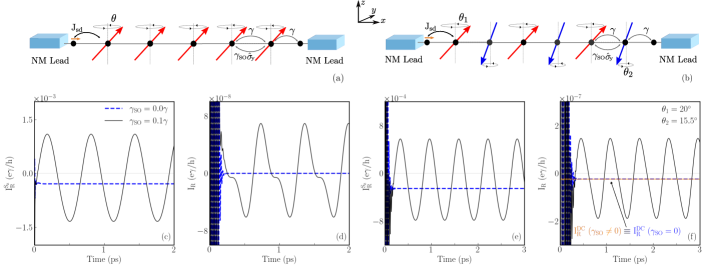
Figure 1: (a) Schematic view of a ferromagnetic metal, modeled on 1D TB lattice of $N=9$ sites (five ferromagnetic sites are shown in the illustration), which is attached to two NM leads modeled as semi-infinite TB chains. Its classical localized magnetic moments $\mathbf{M}_{i}(t)=\big{(}\sin\theta\cos(\omega_{0}t),\sin\theta\sin(\omega_{0}t),\cos\theta\big{)}$ (red arrows) are steadily precessing with frequency $\hbar\omega_{0}=0.01\gamma$ and precession cone angle $\theta=20^{\circ}$ around the $z$-axis due to assumed resonant absorption of microwaves. The conduction electrons within the chain interact with $\mathbf{M}_{i}$ via $sd$ exchange interaction of strength $J_{sd}=0.1\gamma$ and they also experience the Rashba SO coupling [13], so that their Hamiltonian is given by $\hat{H}(t)=-\gamma\sum_{\langle ij\rangle}\hat{c}_{i}^{\dagger}\hat{c}_{j}-i\gamma_{\mathrm{SO}}\sum_{\langle ij\rangle}\hat{c}_{i}^{\dagger}\hat{\sigma}_{y}\hat{c}_{j}-J_{\mathrm{sd}}\sum_{i}\hat{c}_{i}^{\dagger}\hat{\bm{\sigma}}\cdot\mathbf{M}_{i}(t)\hat{c}_{i}$. Here $\hat{c}_{i}^{\dagger}=(\hat{c}_{i\uparrow}^{\dagger}\ \ \hat{c}_{i\downarrow}^{\dagger})$ is a row vector containing operators $\hat{c}_{i\sigma}^{\dagger}$ which create an electron with spin $\sigma=\uparrow,\downarrow$ at site $i$; $\hat{c}_{i}$ is a column vector containing the corresponding annihilation operators; $\gamma$ is the hopping parameter between nearest-neighbor sites; $\gamma_{\mathrm{SO}}$ is an additional spin-dependent hopping [26] due to the Rashba SO coupling [13]; and $\hat{\bm{\sigma}}=(\hat{\sigma}_{x},\hat{\sigma}_{y},\hat{\sigma}_{z})$ is by the vector of the Pauli matrices. In the absence of any bias voltage between macroscopic reservoirs into which NM leads terminate, dynamics of localized magnetic moments $\mathbf{M}_{i}(t)$ drives conduction electrons out of equilibrium so that they comprise pumped (b) spin $I^{S_{z}}_{p}(t)$ [other two components $I^{S_{x}}_{p}(t)$ and $I^{S_{y}}_{p}(t)$ are also nonzero but not shown] and (c) charge $I_{p}(t)$ currents plotted in the right NM lead $p=R$. At $t=0$, electrons are described by the grand canonical equilibrium density matrix [4] and $\mathbf{M}_{i}$ start to precess leading to transient currents at early times in panels (b) and (c), while perfectly periodic [or constant [2], like blue dashed lines at zero SO coupling] currents are established at sufficiently long times. Panels (d)–(f) are counterparts of panels (a)–(c) for antiferromagnetic metal of $N=10$ sites [six antiferromagnetic sites are shown as the illustration in (d)].

A close inspection of Fig. 3 in Ref. [1] reveals that computed charge current is manifestly not periodic, with deviation from periodic function and sudden onset of high frequency embedded signal becoming more conspicuous with increasing SO coupling. This suggests numerical artifacts in the code or its algorithms selected as one increases SO coupling. While nonperiodic currents pumped by time-dependent quantum systems are sometimes reported in the literature (see, e.g., Fig. 1(d) in Ref. [19]), this is invariable related to the usage of a finite-size quantum system with discrete energy spectrum. Once semi-infinite NM leads are attached—so that the whole system active region + NM leads has continuous energy spectrum, which plays a key role in in nonequilibrium quantum statistical mechanics as it provides effective dissipation [20, 21]—perfectly periodic spin $I^{S_{\alpha}}_{p}(t)=I^{S_{\alpha}}_{p}(t+2\pi/\omega_{0})$ and charge $I_{p}(t)=I_{p}(t+2\pi/\omega_{0})$ currents are ensured in the long time limit. This is illustrated by Fig. 1(b) [Fig. 1(e)] for spin and by Fig. 1(c) [Fig. 1(f)] for charge currents pumped into semi-infinite right (R) NM lead of 1D FM [AFM] systems in Fig. 1(a) [Fig. 1(d)] we choose as examples. Thus, the authors citing Ref. [19], where no leads and continuous energy spectrum were used, to justify nonperiodic features of their currents is due to misunderstanding of the properties of the result that TKWANT must produce when properly employed on harmonically driven quantum systems attached to semi-infinite leads.

The second theorem violated by the results of Fig. 3 in Ref. [1] is more subtle and has to do with the key requirement to obtain the DC component, $I_{p}^{\mathrm{DC}}=\frac{1}{\tau}\int_{0}^{\tau}I_{p}(t)dt\neq 0$ where $\tau=2\pi/\omega_{0}$ is one period, of pumped charge current. Note that

$$I_{p}(t) = I_{p}^{\mathrm{DC}}+\sum_{N=1}^{\infty}[(I_{p,N}+I_{p,-N})\cos(N\omega_{0}t)$$ (1)

$$+i(I_{p,N}-I_{p,-N})\sin(N\omega_{0}t)],$$

where $|I_{p,N}|$ is the $N$th harmonic of charge current flowing into lead $p$ that was extracted from FFT of $I_{p}(t)$ in Ref. [1]. The number of non-negligible harmonics and their magnitude can be alternatively, as well as more accurately [14], obtained from the Floquet scattering matrix [15, 16, 17, 14]. For $I_{p}^{\mathrm{DC}}\neq 0$ to happen, the left-right symmetry of a two-terminal device must be broken [22, 15, 23, 24]. For example, if the left-right symmetry is broken by both inversion and time-reversal symmetries being violated dynamically, such as by standard example of two spatially separated potentials oscillating out-of-phase [5], one finds $I_{p}^{\mathrm{DC}}\propto\omega_{0}$ (termed adiabatic pumping) in the low frequency regime. In contrast, if only one of those two symmetries is broken, and this does not have to occur dynamically, then $I_{p}^{\mathrm{DC}}\propto\omega_{0}^{2}$, termed nonadiabatic pumping [22, 15, 23, 24] (e.g., just by adding nonzero on-site potential at one site of the device in Fig. 1(a) would statically break [24] the left-right symmetry and produce $I_{p}^{\mathrm{DC}}\propto\omega_{0}^{2}$ [25]). Thus, perfectly left-right symmetric device in Fig. 1(a) is expected to exhibit $I_{p}^{\mathrm{DC}}\equiv 0$, as confirmed by Fig. 1(c) both in the absence or presence of SO coupling.

Figure 3(a) of Ref. [1] for very small SO coupling does show $I_{p}^{\mathrm{DC}}=0$ [i.e., drawing horizontal line at zero shows that oscillatory current in Fig. 3(a) is symmetric with respect to this line]. But the authors use AFM in which case one actually expects $I_{p}^{\mathrm{DC}}\neq 0$, as confirmed by our example in Fig. 1(f). This is because AFM depicted in Fig. 1(d) breaks the left-right symmetry [there is red LMM on the left edge and blue LMM on the right edge of the active region in Fig. 1(f)]. Further problem with Fig. 3 of Ref. [1] is that $I_{p}^{\mathrm{DC}}\neq 0$ turns nonzero in Fig. 3(b)–(d) with increasing SO coupling while changing its magnitude for different values of SO coupling in panels (b) to (d). Since $I_{p}^{\mathrm{DC}}\neq 0$ means finite transmitted charge into the external circuit, which can do useful work as an example of photovoltaic effect (i.e., generation of DC current by radiation of a finite frequency [22]), Fig. 3(b)–(d) are essentially reporting violation of the conservation of energy, suggesting the trouble with the code. The correct calculation on any AFM system must produce $I_{p}^{\mathrm{DC}}\neq 0$ that is insensitive to the value of the SO coupling, as confirmed by the example in Fig. 1(f) where we denote explicitly $I_{p}^{\mathrm{DC}}(\gamma_{\mathrm{SO}}\neq 0)\equiv I_{p}^{\mathrm{DC}}(\gamma_{\mathrm{SO}}=0)$.

In general, the origin of two violations produced by time-dependent computational quantum transport employed in Ref. [1] could be either due to “bugs” in the software or improper selection of its algorithms. For example, time-dependent currents in TKWANT are obtained by integrating over energy an expression involving auxiliary wavefunctions [27], where bound states have to located [28] on the energy axis and their contributions added manually [12, 29]. Ref. [1] does mention that “evaluation of these integrals constitutes the most demanding task of the calculations” but the issue of bound state contributions is never discussed. These states do not contribute to current in the absence of SO coupling, buy they start to contribute [30] to it once the SO coupling is switched on. Since this is precisely how Fig. 3 of Ref. [1] starts to violate two theorems, i.e., with increasing SO coupling, it is possible that TKWANT is “bug”-free but the authors of Ref. [1] have simply not included all contributions from bound states and/or converged energy integrals [29] (whose integrands can be highly spiky function [27]). Additional pitfalls one can encounter when performing ${\tt TKWANT}$ simulations are discussed in its manual [29].

We note that the need to verify and validate complex scientific software has been recognized long ago [31, 32], and the software and validation procedures have become only more intricate since then [33, 34]. This includes a possibility that combination of different modules within the software could be wrong even if individual modules are well-tested. Otherwise blind trust in the code can lead to huge financial losses, as exemplified by seismic codes motivating drilling for oil in incorrect spots or computationally designed aircrafts that fail testing in real-world wind tunnels. While it is highly unlikely that improperly validated time-dependent quantum transport codes will generate huge financial losses for nanoelectronic or spintronic industry, they could lead to proliferation of apparently fantastic but incorrect results in the physics literature where the arguments with the referees will be settled by saying “we believe in the code” instead of empirical testing and rigorous attention to details at the core of the success of modern science [35].

When experimental data are available, they offer the most effective validation strategy [32]. When both experimental data and exactly solvable examples are absent, one usually resorts to validation based on “code benchmarking” where the results of many different codes for a single problem are compared in order to determine the reasons for divergence [32], as pursued in computational materials science [33, 34]. Here we propose validation strategy tailored for time-dependent quantum transport codes:

• Using simple example, such as 1D TB chain with time-dependent on-site potentials, confirm that code results satisfy two basic theorems explained above, as illustrated by validation performed in Fig. 4 of Ref. [24].

• Compare code with an example with the exact analytical solution. This typically means focusing on quantum system driven by time-periodic external fields. For the case of spin pumping, such an example is provided by a single precessing spin within an infinite 1D TB chain whose analytical formula [25] for pumped spin and charge currents has been reproduced (see, e.g., Fig. 6 in Ref. [4]) in the process of validation of the code employed in Fig. 1, as well as by using TKWANT [30].

• However, exact analytical solution of Ref. [25] cannot be generalized in the presence of SO coupling. Since SO coupling brings new physics and thereby demand on the selection of proper algorithms, code used in Fig. 1 or code used in Fig. 3 of Ref. [1] could be validated for nonzero SO coupling $\gamma_{\mathrm{SO}}$ by time-independent numerical calculations within the Floquet formalism [16] where numerically exact solution is easily achieved by increasing the size [14] of truncated matrices that are otherwise infinite [36] in the Floquet formalism. For this purpose one can also employ KWANT package [37] for time-independent computational quantum transport, where Floquet scattering matrix [15, 16, 17, 14] can be extracted directly from KWANT. We also note that finding precise cutoff harmonic order $N_{\mathrm{max}}$ via time-dependent quantum transport and FFT of its results, as employed in Ref. [1], is very difficult to achieve [14] due to numerical artifacts easily introduced by the choice of time step and FFT window. On the other hand, KWANT calculations of Floquet scattering matrix and pumped currents expressed by it can yield precise [14] number of high harmonics from magnetic systems with precessing magnetization.

In conclusion, we reexamined the problem of current pumping by precessing magnetization in the presence of SO coupling that was very recently explored in Ref. [1], using open source package TKWANT [12] for time-dependent computational quantum transport, to predict implausibly large number of high harmonics in pumped current. We explain that the results of Ref. [1] violate two basic theorems of time-dependent quantum transport, and we also use simple examples [Figs. 1(a) and  1(d)] and a completely different computational scheme [4] to demonstrate how the correct results [panels (b),(c),(e) and (f) of Fig. 1] must obey both theorems. Thus, the claim of “ultrahigh” harmonic number in Ref. [1] appears to be an artifact of either “bugs” or incorrectly selected algorithms within TKWANT package. Regarding the latter possibility, let us recall that in teaching of elementary Computational Physics [38] students are exposed early to the Euler algorithm for discretization of ordinary differential equations, as well as to its failure for oscillatory problems where it generates unphysical monotonically increasing energy with time. One then learns a simple fix to the Euler algorithm by switching to the Euler-Cromer one [38]. The same approach—looking for violation of energy conservation—is also often used to select proper algorithms for much more complicated quantum time evolution [39]. Usage of the first of two theorems discussed above is of the same type, but the second one is far less obvious. Even if both theorems are satisfied, one should still perform additional testing of code accuracy, as exemplified by recent extensive efforts in computational materials science to compare large number of codes [33, 34].

For time-dependent quantum transport codes, this can be accomplished by comparing code results with an analytical formula, or with numerically exact results obtained independently of a chosen code, for one or more carefully chosen testbed systems. As suggested above, a single testbed system would not be sufficient to validate accuracy of calculations of Ref. [1] due to completely different demand on the selection of algorithms within TKWANT for zero vs. nonzero SO coupling. A user of open source scientific software who spends time to run carefully chosen testbed example (such as the three items suggested above), instead of running software as a black box, could evade blind reporting of invalid results due to subtle issues [32] like software components combined could be wrong even though the components test well individually; or a software combination that is insensitive to minor component errors but still gives an invalid results.

- [1] O. Ly and A. Manchon, Spin-orbit coupling induced ultrahigh-harmonic generation from magnetic dynamics, Phys. Rev. B 105, L180415 (2022).
- [2] Y. Tserkovnyak, A. Brataas, G. E. W. Bauer, and B. I. Halperin, Nonlocal magnetization dynamics in ferromagnetic heterostructures, Rev. Mod. Phys. 77, 1375 (2005).
- [3] K. Ando, Dynamical generation of spin currents, Semicond. Sci. Technol. 29, 043002 (2014).
- [4] M. D. Petrović, B. S. Popescu, U. Bajpai, P. Plecháč, and B. K. Nikolić, Spin and charge pumping by a steady or pulse-current-driven magnetic domain wall: A self-consistent multiscale time-dependent quantum-classical hybrid approach, Phys. Rev. Appl. 10, 054038 (2018).
- [5] P. W. Brouwer, Scattering approach to parametric pumping, Phys. Rev. B 58, R10135 (1998).
- [6] F. Mahfouzi, J. Fabian, N. Nagaosa, and B. K. Nikolić, Charge pumping by magnetization dynamics in magnetic and semimagnetic tunnel junctions with interfacial Rashba or bulk extrinsic spin-orbit coupling, Phys. Rev. B 85, 054406 (2012).
- [7] K. Chen and S. Zhang, Spin pumping in the presence of spin-orbit coupling, Phys. Rev. Lett. 114, 126602 (2015).
- [8] C. Ciccarelli, K. M. D. Hals, A. Irvine, V. Novak, Y. Tserkovnyak, H. Kurebayashi, A. Brataas, and A. Ferguson, Magnonic charge pumping via spin–orbit coupling, Nat. Nanotech. 10, 50 (2015).
- [9] A. Ahmadi and E. R. Mucciolo, Microscopic formulation of dynamical spin injection in ferromagnetic-nonmagnetic heterostructures, Phys. Rev. B 96, 035420 (2017).
- [10] K. Dolui, U. Bajpai, and B. K. Nikolić, Effective spin-mixing conductance of topological-insulator/ferromagnet and heavy-metal/ferromagnet spin-orbit-coupled interfaces: A first-principles Floquet-nonequilibrium Green function approach, Phys. Rev. Mater. 4, 121201(R) (2020).
- [11] K. Dolui, A. Suresh, and B. K. Nikolić, Spin pumping from antiferromagnetic insulator spin-orbit-proximitized by adjacent heavy metal: A first-principles Floquet-nonequilibrium Green function study, J. Phys. Mater. 5, 034002 (2022).
- [12] T. Kloss, J. Weston, B. Gaury, B. Rossignol, C. Groth, and X. Waintal, TKWANT: a software package for time-dependent quantum transport, New J. Phys. 23 023025 (2021).
- [13] A. Manchon, H. C. Koo, J. Nitta, S. M. Frolov, and R. A. Duine, New perspectives for Rashba spin–orbit coupling, Nat. Mater. 14, 871 (2015).
- [14] J. V. Manjarres and B. K. Nikolić, High-harmonic generation in spin and charge current pumping at ferromagnetic or antiferromagnetic resonance in the presence of spin-orbit coupling, arXiv:2112.14685.
- [15] M. Moskalets and M. Büttiker, Floquet scattering theory of quantum pump, Phys. Rev. B 66, 205320 (2002).
- [16] M. V. Moskalets, Scattering Matrix Approach to Non-Stationary Quantum Transport (Imeprial College Press, London, 2011).
- [17] L. Arrachea and M. Moskalets, Relation between scattering-matrix and Keldysh formalisms for quantum transport driven by time-periodic fields, Phys. Rev. B 74, 245322 (2006).
- [18] M. Lysne, Y. Murakami, M. Schüler, and P. Werner, High-harmonic generation in spin-orbit coupled systems, Phys. Rev. B 102, 081121(R) (2020).
- [19] S. Imai, A. Ono, and S. Ishihara, High harmonic generation in a correlated electron system, Phys. Rev. Lett. 124, 157404 (2020).
- [20] G. Giuliani and G. Vignale, Quantum Theory of the Electron Liquid (Cambridge University Press, Cambridge, 2012).
- [21] A. Brataas, Y. Tserkovnyak, and G. E. W. Bauer, Scattering theory of Gilbert damping, Phys. Rev. Lett. 101, 037207 (2008).
- [22] M. G. Vavilov, V. Ambegaokar, and I. L. Aleiner, Charge pumping and photovoltaic effect in open quantum dots, Phys. Rev. B 63, 195313 (2001).
- [23] L. E. F. Foa Torres, Mono-parametric quantum charge pumping: Interplay between spatial interference and photon-assisted tunneling, Phys. Rev. B 72, 245339 (2005).
- [24] U. Bajpai, B. S. Popescu, P. Plecháč, B. K. Nikolić, L. E. F. Foa Torres, H. Ishizuka, and N. Nagaosa, Spatio-temporal dynamics of shift current quantum pumping by femtosecond light pulse, J. Phys.: Mater. 2, 025004 (2019).
- [25] S.-H. Chen, C.-R. Chang, J. Q. Xiao, and B. K. Nikolić, Spin and charge pumping in magnetic tunnel junctions with precessing magnetization: A nonequilibrium Green function approach, Phys. Rev. B. 79, 054424 (2009).
- [26] B. K. Nikolić, L. P. Zârbo, and S. Souma, Imaging mesoscopic spin Hall fow: Spatial distribution of local spin currents and spin densities in and out of multiterminal spin-orbit coupled semiconductor nanostructures, Phys. Rev. B 73, 075303 (2006).
- [27] B. Gaury, J. Weston, M. Santin, M. Houzet, C. Groth, and X. Waintal, Numerical simulations of time-resolved quantum electronics, Phys. Rep. 534, 1 (2014).
- [28] M. Istas, C. Groth, A. R. Akhmerov, M. Wimmer, and X. Waintal, A general algorithm for computing bound states in infinite tight-binding systems, SciPost Phys. 4, 026 (2018); see also TKWANT manual, https://tkwant.kwant-project.org/doc/dev/tutorial/boundstates.html.
- [29] https://tkwant.kwant-project.org/doc/dev/tutorial/pitfalls.html
- [30] T. Kloss, private communication.
- [31] L. Hatton, The T experiments: errors in scientific software, IEEE Comput. Sci. Eng. 4, 27 (1997).
- [32] D. Post and L. Votta, Computational science demands a new paradigm, Phys. Today 58, 35 (2005).
- [33] K. Lejaeghere et al., Reproducibility in density functional theory calculations of solids, Science 351, aad3000 (2016).
- [34] T. Vogel, S. Druskat, M. Scheidgen, C. Draxl, and L. Grunske, Challenges for verifying and validating scientific software in computational materials science, 2019 IEEE/ACM 14th International Workshop on Software Engineering for Science (SE4Science), 25 (2019); also available as arXiv:1906.09179.
- [35] M. Strevens, The Knowledge Machine: How Irrationality Created Modern Science (Liveright, New York, 2020).
- [36] A. Eckardt and E. Anisimovas, High-frequency approximation for periodically driven quantum systems from a Floquet-space perspective, New J. Phys. 17, 093039 (2015).
- [37] C. W. Groth, M. Wimmer, A. R. Akhmerov, and X. Waintal, Kwant: a software package for quantum transport, New J. Phys. 16, 063065 (2014).
- [38] N. J. Giordano and H. Nakanishi, Computational Physics (Pearson Prentice Hall, Upper Saddle River, 2006).
- [39] N. Hatano and M. Suzuki, Finding exponential product formulas of higher orders, arXiv:math-ph/0506007.