Fundamentals of Perpetual Futures

Abstract

Perpetual futures—swap contracts that never expire—are the most popular derivative traded in cryptocurrency markets, with more than $100 billion traded daily. Perpetuals provide investors with leveraged exposure to cryptocurrencies, which does not require rollover or direct cryptocurrency holding. To keep the gap between perpetual futures and spot prices small, long position holders periodically pay short position holders a funding rate proportional to this gap. The funding rate incentivizes trades that tend to narrow the futures-spot gap. But unlike fixed-maturity futures, perpetuals are not guaranteed to converge to the spot price of their underlying asset at any time, and familiar no-arbitrage prices for perpetuals are not available, as the contracts have no expiry date to enforce arbitrage. Here, using a weaker notion of random-maturity arbitrage, we derive no-arbitrage prices for perpetual futures in frictionless markets and no-arbitrage bounds for markets with trading costs. These no-arbitrage prices provide a valuable benchmark for perpetual futures and simultaneously prescribe a strategy to exploit divergence from these fundamental values. Empirically, we find that deviations of crypto perpetual futures from no-arbitrage prices are considerably larger than those documented in traditional currency markets. These deviations comove across cryptocurrencies and diminish over time as crypto markets develop and become more efficient. A simple trading strategy generates large Sharpe ratios even for investors paying the highest trading costs on Binance, which is currently the largest crypto exchange by volume. JEL Classification: G11, G12, G13
Keywords: Perpetual futures, crypto, random-maturity arbitrage, funding rate

1 Introduction

Perpetual futures are, by far, the most popular derivative traded in cryptocurrency markets, generating a daily volume of more than $100 billion. Prior to the recent collapse of FTX, perpetual futures were among the most actively-traded products on the exchange, with the now-bankrupt hedge fund Alameda Research taking the other side of many such leveraged trades. Despite their central role in crypto markets, there is relatively little work studying these derivatives. In this paper we ask: what are the theoretical fundamental values of perpetual futures, and how large are deviations from these fundamentals empirically?

Perpetuals are derivatives that allow investors to speculate on or hedge against cryptocurrency price fluctuations using high leverage, without needing to acquire the cryptocurrencies or to roll them over. Like traditional fixed-maturity futures, at initiation, a long and short counterparty agree on an initial futures price without exchanging any money, other than posting margin with the exchange. Both parties can enter or exit the contract at any time, with profits or losses continuously calculated and allocated to each side’s margin account based on the prevailing market prices.

Unlike fixed-maturity futures, perpetuals do not expire. This feature enhances the liquidity of the contract, as there is no staggering of contracts with different maturities traded on the exchange, and only a single perpetual futures contract per underlying asset is listed. Moreover, this instrument does not require market participants to deal with the rolling over of their futures positions and is traded 24/7.

Because they have no set expiration date, perpetuals are not guaranteed to converge to the spot price of their underlying asset at any given time, and the usual no-arbitrage prices for perpetuals are not applicable. To minimize the gap between perpetual futures and spot prices, long position holders periodically pay short position holders a ’funding rate’ proportional to this gap to incentivize trades that narrow it. For example, when the futures price exceeds the spot price, arbitrageurs who borrow cash to long the spot and simultaneously short the futures would receive the funding rate. Their trades would tend to increase the spot price and decrease the futures price. A narrow gap means that perpetual futures offer effective exposure to variation in the spot price of the underlying asset to hedging and speculating investors. Typically, the funding rate is paid every eight hours and approximately equals the average futures-spot spread over the preceding eight hours. Note that the strategy just sketched, commonly referred to as ’funding rate arbitrage,’ is not risk-free even disregarding margin requirements and trading costs, simply because there is no predetermined expiration date when the trade would be unwound at a profit.

We derive no-arbitrage prices for perpetual futures in frictionless markets and derive no-arbitrage bounds in markets with trading costs. The theoretical perpetual futures price is proportional to the spot price of the underlying, with a constant of proportionality that increases in the ratio of the interest rate to a constant that determines the magnitude of the funding rate. The interest rate captures the cost of borrowing cash to finance holding the underlying, while the funding rate captures the benefit of shorting the futures. Thus, intuitively, the future-spot spread is larger when the cash borrowing interest rate is large relative to the funding rate.

Our derivation relies on a weaker notion of arbitrage that we call random-maturity arbitrage. As its name suggests, unlike traditional riskless arbitrage, we allow the strategy’s time-to-maturity to be random. At first glance, one might object that such prices are not truly based on riskless arbitrage. Note, however, that riskless no-arbitrage pricing is usually just a useful fiction (Pedersen, 2019). For example, in real-world futures markets, arbitrageurs must maintain a margin account during the entire period in which the arbitrage trade is open. Temporary worsening of apparent arbitrage opportunities can lead to liquidations and losses. As the saying goes, an arbitrageur must remain liquid longer than the market stays irrational. Thus, even arbitrage opportunities that appear to be riskless in theory, may be risky in practice.

These no-arbitrage prices provide a useful benchmark for perpetual futures and simultaneously prescribe a strategy to exploit divergence from these fundamental values. Motivated by the theoretical understanding, we study the empirical deviations of the perpetual futures price from the spot. We find that the mean deviation from our benchmark is modest and statistically insignificant, which suggests that it is a useful benchmark for futures prices.

Around this benchmark, however, perpetual futures often differ significantly from spot prices. The mean absolute deviation is about 60% to 100% per year across different cryptocurrencies, which is considerably larger than the deviations documented in traditional currency markets by Du, Tepper, and Verdelhan (2018). We find strong comovement of the futures-spot gap across different cryptocurrencies. This comovement can be due to commonality in funding and market liquidity faced by arbitrageurs who operate in multiple cryptocurrencies. Common sentiment could also drive the difference in futures demand relative to the spot. Overall, the deviation’s magnitude is comparable to our theoretic no-arbitrage bound calibrated to actual trading fees.

These deviations narrows considerably in 2022, suggesting a decrease in arbitrage frictions in the market and an increase in competition among arbitrageurs. The narrowing gap provides an additional perspective on the downfall of Alameda Research and Three Arrows Capital. According to news reports and interviews, both hedge funds seem to have pivoted from such arbitrage activity around late 2021 to early 2022 and started taking more directional bets on cryptocurrencies, with both direct unhedged crypto holdings and investments in crypto startups. The large declines in crypto prices in 2022 subsequently exhausted their capital and led to their bankruptcies.

To understand the economics of the futures-spot spread, we consider a trading strategy motivated by the random-maturity arbitrage theory. Whenever the futures-spot spread exceeds the theoretical bound under certain trading cost tiers, we open the trading position and close it when the futures-spot spread returns to its theoretical relationship under no trading costs. We find that empirically, the random maturity arbitrage strategy generates a sizable Sharpe ratio even under high trading costs. For example, for Bitcoin perpetual futures, the strategy generates a Sharpe ratio of 1.92 under high trading costs typical of retail investors, and up to 3.94 for highly-active market makers who pay no such fees. The strategy’s performance is even better for Ether and other cryptocurrencies and deliver significant alphas relative to the 3-factor model of Liu, Tsyvinski, and Wu (2022) and the 5-factor model of Cong, Karolyi, Tang, and Zhao (2022b).

What explains these large no-arbitrage deviations? One natural explanation is that liquidity in crypto markets is insufficient for arbitrageurs to eliminate such violations. Our finding that the spreads decline over time is consistent with liquidity improving as these markets develop, and leaves open the possibility that they will narrow going forward. We also find, however, that past return momentum significantly explains the futures-spot gap with a time-series regression $R^{2}$ of more than $50\%$. When past returns are high, futures tend to trade at a higher price relative to the spot. This indicates positive feedback or momentum trading behavior in the perpetual futures market. This correlation may linger even as crypto markets become more efficient.

The existing literature on perpetual futures mainly focuses on descriptive evidence. See e.g. Alexander, Choi, Park, and Sohn (2020), Schmeling, Schrimpf, and Todorov (2022), De Blasis and Webb (2022), Ferko, Moin, Onur, and Penick (2022), and Streltsov and Ruan (2022). Angeris, Chitra, Evans, and Lorig (2022) provide a theoretical no-arbitrage analysis of perpetuals, but they make over-simplifying assumptions by assuming the payoff from the perpetual is a fixed function of the underlying spot price. Compared to the existing literature, we illustrate the fundamental mechanism behind the perpetual design and derive theoretical no-arbitrage prices and bounds for this instrument.

Also related is recent literature on fixed maturity futures in the crypto space. Schmeling, Schrimpf, and Todorov (2022) provides a comprehensive analysis of the carry of crypto futures, with the carry defined following the general definition of Koijen, Moskowitz, Pedersen, and Vrugt (2018). Schmeling, Schrimpf, and Todorov (2022) document a volatile convenience yield in the crypto space driven by high leverage from trend-chasing small investors and the relative scarcity of arbitrage capital. Cong, He, and Tang (2022a) provide a novel link of the volatile convenience yield to the staking, service flow, and transaction convenience of the underlying tokens. They show that the large deviation from uncovered interest rate parity can be reconciled with transaction convenience. Our paper focuses on perpetual futures rather than fixed maturity futures and extends fixed-maturity to random-maturity no-arbitrage pricing.

More broadly, our paper contributes to the understanding of the frictions and arbitrage in cryptocurrency markets. Makarov and Schoar (2020) study price deviations across exchanges. They find large gaps across countries, highlighting the important role played by capital controls and slow-moving arbitrage capital as in Duffie (2010). Our analysis focuses on the price wedge between the spot and the futures market. We find that even within an exchange, futures prices deviate from their theoretical arbitrage-free values. These results indicate there are significant limits to arbitrage as in Gromb and Vayanos (2018) for cryptocurrencies in the early years.

The rest of the paper is organized as follows: Section 2 provides the institutional details and history of perpetual futures. Section 3 presents the no-arbitrage analysis of the perpetual futures market and derives the theoretical price of perpetual futures. Section 4 demonstrates the empirical futures-spot deviation and presents the simple theory-motivated trading strategy that can exploit the arbitrage opportunity. Section 5 provides some explanation for the deviation between futures and the spot. Section 6 concludes.

2 An Introduction to Perpetual Futures

The idea of perpetual futures was first introduced by Shiller (1993). The goal was to set up a perpetual claim on the cash flows of an illiquid asset. For example, the underlying illiquid asset could be a house which generates rents as cash flows. The purpose of the perpetual futures is to enable price discovery for the underlying with an illiquid or hard-to-measure price. Perpetual futures have no expiration date but cash is exchanged between the long and the short side: after buying the perpetual futures, the long side is entitled to receive the flow cash flow from the short side and they settle the price difference when exiting the position.

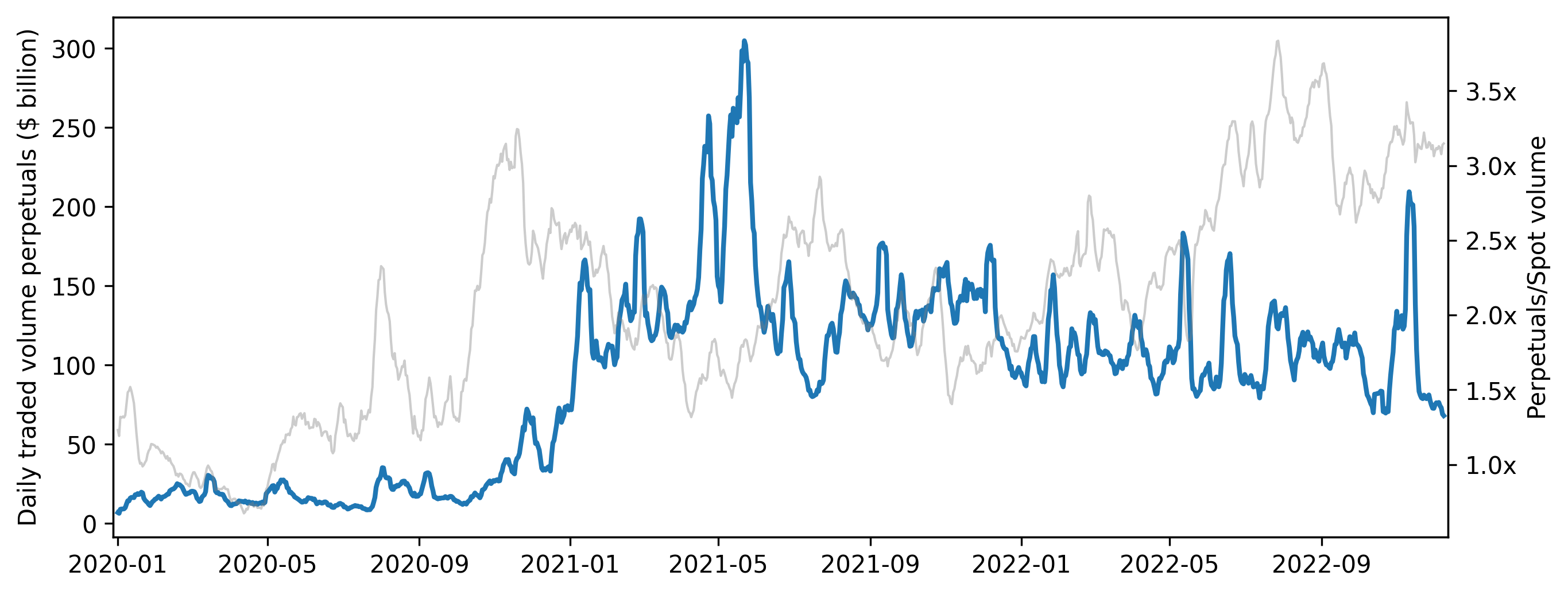
Figure 1: Total trading volumes of perpetual futures across exchanges

The figure displays the 7-day moving average daily traded volume for perpetual futures across all exchanges in blue. The median daily volume is $17.8 bn. (2020), $132.0 bn. (2021) and $101.9 bn. (2022). This translates to a yearly volume of $8,551 bn. (2020), $51,989 bn. (2021) and $39,306 bn. (2022) respectively. Additionally, the grey line depicts the ratio between the traded volume in perpetuals and spot markets. In 2022 the Perpetual markets are consistently trading between 2x or 3.5x the spot volume. The data is obtained from CoinGecko, a crypto data specialist. We exclude exchanges that are known for misrepresenting data (e.g. forms of wash trading).

Perpetual futures in crypto markets similarly have no expiration date and cash is exchanged between the long and the short side, but their purpose is different from Shiller’s original idea. First, unlike, e.g. real estate market, crypto has no inherent dividend or cash flow. Second, the price discovery argument of Shiller is most applicable to settings where spot prices are difficult to measure. Crypto spot prices, however, can be measured from active trading on different exchanges, and decentralized exchanges such as Bancor (Hertzog et al., 2017) or Uniswap (Adams et al., 2021) offer price discovery for assets with minimal liquidity. The major role perpetual futures play in the crypto space is to offer an effective leveraged trading vehicle to hedge or speculate the underlying spot price movement, which makes the market more complete. It also serves as an effective tax payment optimization tool for investors.

Crypto perpetual futures were first introduced by BitMEX in 2016, which gained great popularity in the crypto space since its inception. It initially served as an effective hedging tool for crypto miners. It was later adopted by crypto speculators interested in leveraged exposure. Nowadays, based on data from CoinGecko, the median total daily trading volume of perpetual futures across all exchanges is 101.9 billion in the year 2022 which is about $2\times$ to $3\times$ the total spot trading volume across these exchanges. Figure 1 presents the 7-day moving average of the total trading volume of perpetual futures across all exchanges. We see a significant rise in trading of perpetual futures around January 2021 and the total volume stabilizes at a level above $100 billion per day following the rise.

Cong, Li, Tang, and Yang (2022c) document significant wash trading behavior among crypto exchanges because of competition, the ranking mechanism, and lack of regulation. They estimate that over 70% of crypto trading volume is not real. Amiram, Lyandres, and Rabetti (2021) confirm this conclusion using new data and an extended methodology. Therefore, in calculating trading volume, we exclude exchanges that are known to misrepresent data.

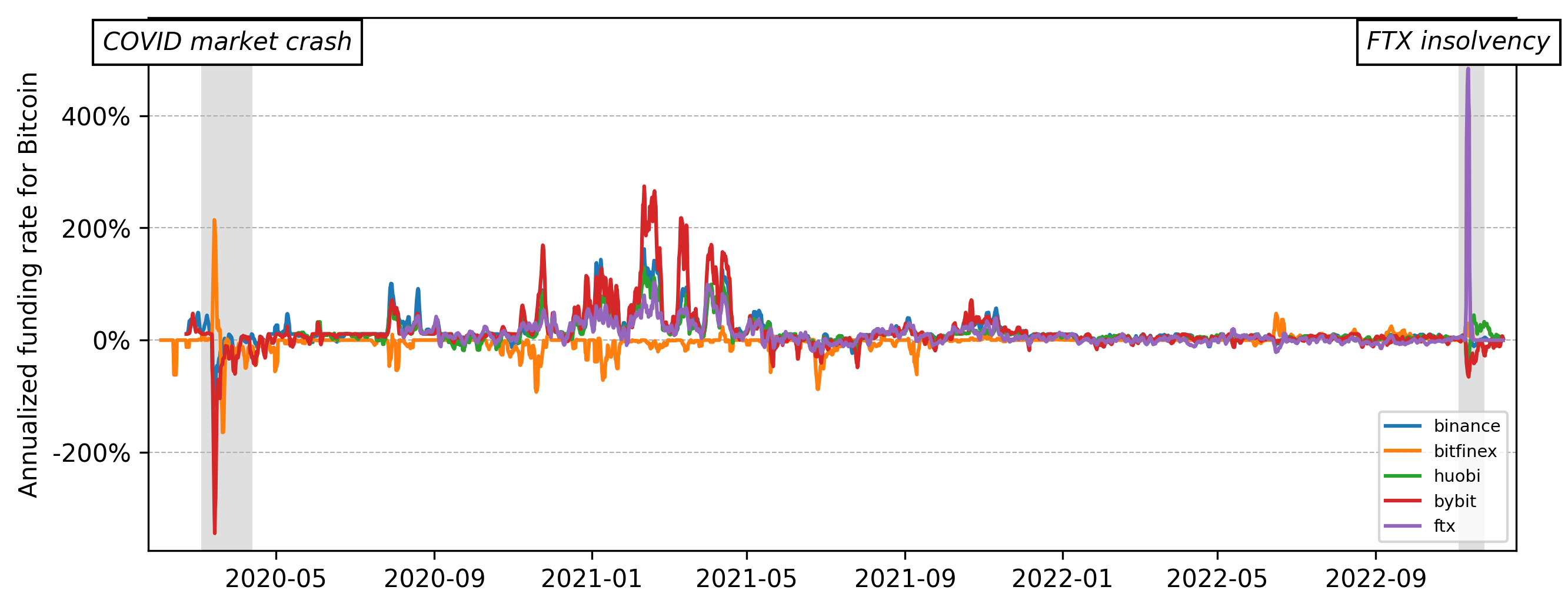
Figure 2: Bitcoin annualized funding rate across exchanges

The figure presents the 7-day moving average annualized funding rate for Bitcoin (BTC) across exchanges. The data is obtained from glassnode, an analytics platform. The data covers two major market turbulences: the COVID stock market crash from February to April 2020, and the FTX insolvency in November 2022. The FTX collapse led to significant negative funding rates on all solvent exchanges, thus the perpetual future prices were lower than the spot prices on the solvent exchanges. Vice versa on the insolvent FTX. The funding rates become more volatile after the event, indicating increased uncertainty for the market participants.

A key feature of crypto perpetual futures is the funding rate, which is the cash exchanged between the long and short counterparties. Its goal is to keep the futures price close to the underlying spot so that the futures can be an effective hedging tool for spot price movement. The funding rate is typically paid every 8 hours. Its value is approximately a weighted average of the prior 8 hours’ price gap of the futures and the spot. If the futures price is above the spot, the funding rate will be positive, meaning the long side of the futures needs to pay the short side. This incentivizes traders to short the futures, and in doing so, to move its price back in line with the spot. On the other hand, when the futures price is below the spot, the funding rate turns negative, which means the short side needs to pay the long side. Therefore, the funding rate is the key mechanism keeping the futures price close to the spot price. Note that perpetual futures cannot be replicated by rolling over 8-hour maturity futures. For the latter, every 8 hours, the price is guaranteed to converge to the underlying spot, while for the perpetual futures this is not the case.

Figure 2 presents the annualized 7-day moving average of Bitcoin perpetual funding rates across leading exchanges from January 2020 to December 2022. The funding rate is positive when the futures-to-spot spread is positive, and negative otherwise. Funding rates tend to be similar across exchanges due to cross-exchange arbitrage activity, but can diverge during extreme liquidity episodes. During March 2020, as Covid-19 started to spread and liquidity evaporated, funding rates turned substantially negative in most exchanges. Funding rates turned highly positive during the crypto bull run of early 2021. The last episode highlighted is the collapse of FTX, which was the 4th largest crypto exchange at the time. The figure shows that Bitcoin futures prices were substantially higher than spot prices at FTX, but the opposite was true on other exchanges. This pattern is consistent with FTX investors liquidating their short futures positions quickly, either voluntarily to reduce their exposure to the failing exchange, or involuntarily as the exchange liquidated their underfunded positions.

3 Arbitrage in Perpetual Futures

We next derive no-arbitrage prices for perpetual futures prices relative to spot prices. Unlike traditional futures, perpetual futures have no expiration date. To analyze arbitrage in this market, we extend the traditional notion of risk-free arbitrage where arbitrageurs have a guaranteed positive payoff at a certain time in the future. We first describe the payoff structure of perpetual futures. We then introduce a generalized notion of an arbitrage opportunity with a certain positive payoff but at an uncertain future time.

Definition 1 (Perpetual futures).

A perpetual futures contract $\{F_{t}\}_{t=0}^{\infty}$ written on $\{S_{t}\}_{t=0}^{\infty}$ is an agreement between the long and the short side. There is $0$ cost to enter the agreement. After entering, both the long side and the short side can terminate the contract at any time $t$. Before termination, for each unit of the perpetual, the long must pay the short an $\mathcal{F}_{s}-$adapted cash-flow $\kappa(F_{s}-S_{s})ds,\,s\in(0,t)$, referred to as the funding value. $\kappa$ is a scaling parameter determining the magnitude of the funding rate relative to the price gap. At termination, the short needs to pay the long $F_{t}-F_{0}\,$ for each unit shorted.

This definition is an approximation of real-world perpetual futures. In most exchanges, the funding value for perpetual futures is paid every $8$ hours and approximately equals the average difference between the futures price and the spot over the $8$ hours ($480$ minutes or $\frac{1}{1095}$ years). If we measure time units in years, the cumulative funding rate payment during an 8-hour period is:

$$\int_{t}^{t+1/1095}\kappa(F_{s}-S_{s})ds.$$

Consider the case when $F_{t}-S_{t}=G$, which is constant over the 8-hour interval. In the real world, the funding rate payment would equal $G$ while in our model, the number is $\frac{\kappa G}{1095}$. To equalize the two, we have $\kappa=1095$.

The traditional notions of arbitrage typically consider a guaranteed positive payoff at a certain future date.

Definition 2 (Riskless arbitrage).

A riskless arbitrage opportunity is defined with respect to a payoff $x$ at a certain future time $\tau$ and its price $p(x)$. If the following conditions are satisfied: (1) $x\geq 0$ almost surely, (2) $x>0$ with some positive probability, and (3) its price satisfies $p(x)\leq 0$, then this payoff is an arbitrage opportunity (Cochrane, 2009).

There is no certain future time, however, when a perpetual futures expires and its price is guaranteed to converge to some fixed function of the spot price. Therefore, a generalized notion of arbitrage is required. Suppose the risk-free rate is constant. We define random-maturity arbitrage opportunities as zero-cost strategies with a guaranteed positive payoff at an uncertain future time. Stated formally:

Definition 3 (Random-maturity arbitrage).

A random-maturity arbitrage opportunity is defined with respect to a random payoff $x$ at a future random time $\tilde{\tau}$, $\tilde{\tau}\in(0,\infty)$, and its price $p(x)$. If the following conditions are satisfied: (1) $x\geq 0$ almost surely, (2) $x>0$ with some positive probability, and (3) its price satisfies $p(x)\leq 0$, then this payoff is a random-maturity arbitrage opportunity.

Definition 3 generalizes traditional arbitrage in the sense that there is a guaranteed positive payoff but at an uncertain future time. The following corollary specializes this definition for perpetual futures:

Corollary 1.

In the perpetual futures market, if a strategy (1) has $0$ cost at time $0$, and (2) for any price path of the futures and the spot, $\{F_{t}\}_{t=0}^{\infty}$ and $\{S_{t}\}_{t=0}^{\infty}$, there exists an unwinding time $\tilde{\tau}$ such that its discounted payoff at time $t=\tilde{\tau}$ is positive, then this strategy is a random-maturity arbitrage.

We next show that when there is no random-maturity arbitrage, the gap between futures and spot prices is bounded by a constant. We make the two following assumptions:

Assumption 1.

The gap between the perpetual futures and the spot satisfies the following condition: $\liminf_{t\rightarrow\infty}|F_{t}(\omega)-S_{t}(\omega)|<\infty$, $\forall\,\omega$

Assumption 2.

The risk-free rate $r$ for arbitrageurs is constant.

Assumption 1 is a no-bubble condition. $\liminf$ represents the greatest lower bound as $t\rightarrow\infty$. In other words, we can always find $F_{t}$ and $S_{t}$ that lie within a finite bound as $t\rightarrow\infty$. This condition allows for the gap between $F_{t}$ and $S_{t}$ to explode in the limit as long as it shrinks at some subsequent time. Assumption 2 guarantees that there is no roll-over risk for the arbitrageurs. With these two assumptions, we can state the conclusion as follows.

Proposition 1 (No-arbitrage bound).

Under Assumptions 1 and 2, when there is a constant trading cost $C$ paid when terminating the position, arbitrageurs will trade the perpetual futures until it lies within the following bound relative to the spot:

$$S_{t}\left(1+\frac{r}{\kappa}\right)-C\leq F_{t}\leq S_{t}\left(1+\frac{r}{\kappa}\right)+C\ .$$ (1)

Proof.

Consider the following two scenarios in Table 1. (1) $F_{0}>S_{0}(1+\frac{r}{\kappa})+C$; (2) $F_{0}<S_{0}(1+\frac{r}{\kappa})-C$. We show in the first case, arbitrageurs would long the spot and short the futures because this is a random-maturity arbitrage opportunity. We then show that the opposite strategy is optimal in the second case.

		$F_{0}>S_{0}\left(1+\frac{r}{\kappa}\right)+C$	$F_{0}<S_{0}\left(1+\frac{r}{\kappa}\right)-C$
Actions		Long spot, short futures	Long futures, short spot
	Futures	0	0
Time $0$	Spot	$-S_{0}$	$+S_{0}$
	Cash	$+S_{0}$	$-S_{0}$
Time $t$	Futures	$F_{0}-F_{t}$	$F_{t}-F_{0}$
	Spot	$+S_{t}$	$-S_{t}$
	Cash	$-S_{0}e^{rt}$	$+S_{0}e^{rt}$
	Funding	$\kappa\int_{0}^{t}(F_{s}-S_{s})e^{r(t-s)}ds$	$-\kappa\int_{0}^{t}(F_{s}-S_{s})e^{r(t-s)}ds$
	Trading Cost	$-C$	$-C$
	Payoff	$e^{-rt}F_{0}-e^{-rt}(F_{t}-S_{t})-S_{0}$	$e^{-rt}(F_{t}-S_{t})-e^{-rt}F_{0}+S_{0}$
		$+\kappa\int_{0}^{t}(F_{s}-S_{s})e^{-rs}ds-$	$-\kappa\int_{0}^{t}(F_{s}-S_{s})e^{-rs}ds-$
		$e^{-rt}C$	$e^{-rt}C$

Table 1: Discounted payoffs to arbitrage strategies in perpetual futures and spot markets

This table presents the costs and benefits of two arbitrage trading strategies: (1) when $F_{0}>S_{0}\left(1+\frac{r}{\kappa}\right)+C$, long the spot and short the futures; (2) when $F_{0}<S_{0}\left(1+\frac{r}{\kappa}\right)-C$, long the futures and short the spot. In the last row, the payoff from exiting the position is the discounted payoff from future and spot price changes, proceeds from the cash market, and the funding rate.

Scenario 1: If $F_{0}>S_{0}\left(1+\frac{r}{\kappa}\right)+C$, consider the strategy of longing the spot and shorting the futures. We want to show that for any price path of the perpetual futures and the spot, there exists a future unwinding time $t$ such that the strategy’s payoff is positive, that is, this is a random-maturity arbitrage. Suppose to the contrary that there exists a price path $\{F_{t}\}_{t=0}^{\infty}$ and $\{S_{t}\}_{t=0}^{\infty}$ such that $\forall t$, the discounted payoff from the strategy is negative, or equivalently that:

$$\underbrace{e^{-rt}F_{0}-S_{0}}_{\text{traditional spread}}+\underbrace{\kappa\int_{0}^{t}(F_{s}-S_{s})e^{-rs}ds}_{\text{funding payments}}\leq\underbrace{e^{-rt}(F_{t}-S_{t})}_{\text{spread at unwinding}}+\underbrace{e^{-rt}C}_{\text{trading costs}}.$$ (2)

Denote $(F_{t}-S_{t})e^{-rt}\equiv u_{t}$ the discounted deviation. The inequality becomes:

$$u_{t}\geq e^{-rt}(F_{0}-C)-S_{0}+\kappa\int_{0}^{t}u_{s}ds\ .$$

$\underline{u}_{t}=e^{-rt}(F_{0}-C)-S_{0}+\kappa\int_{0}^{t}\underline{u}_{s}ds$ provides a lower bound for all processes $u_{t}$ satisfying the above inequality. Solving this integral equation, we have:

$$\underline{u}_{t}=\frac{F_{0}re^{-rt}}{\kappa+r}+\left(\frac{F_{0}-C}{1+\frac{r}{\kappa}}-S_{0}\right)e^{\kappa t}\ .$$

When $F_{0}>S_{0}\left(1+\frac{r}{\kappa}\right)+C$, $\lim_{t\rightarrow\infty}\underline{u}_{t}=\infty$. This contradicts Assumption 1, because it implies: $\liminf_{t\rightarrow\infty}(F_{t}-S_{t})e^{-rt}\geq\lim_{t\rightarrow\infty}\underline{u}_{t}\rightarrow\infty$. Therefore, when $F_{0}>S_{0}\left(1+\frac{r}{\kappa}\right)+C$, longing the spot and shorting the futures is a random-maturity arbitrage opportunity.

Scenario 2: Next, if $F_{0}<S_{0}\left(1+\frac{r}{\kappa}\right)-C$, consider the strategy of longing the futures and shorting the spot. As before, we want to show for this strategy, that for any price path of the perpetual futures and the spot, there always exists a future time $t$ such that the strategy payoff is positive, i.e. this is a random-maturity arbitrage. Suppose not, then there exists a price path $\{F_{t}\}_{t=0}^{\infty}$ and $\{S_{t}\}_{t=0}^{\infty}$ such that $\forall t$, the discounted payoff is negative:

$$u_{t}\leq e^{-rt}(F_{0}+C)-S_{0}+\kappa\int_{0}^{t}u_{s}ds\ .$$

$\bar{u}_{t}=e^{-rt}(F_{0}+C)-S_{0}+\kappa\int_{0}^{t}\bar{u}_{s}ds$ provides an upper bound for all processes $u_{t}$ satisfying the above inequality. This is the same integral equation as we see in the first case. We have:

$$\bar{u}_{t}=\frac{F_{0}re^{-rt}}{\kappa+r}+\left(\frac{F_{0}+C}{1+\frac{r}{\kappa}}-S_{0}\right)e^{\kappa t}\ .$$

When $F_{0}<S_{0}\left(1+\frac{r}{\kappa}\right)-C$, $\lim_{t\rightarrow\infty}\bar{u}_{t}=-\infty$. This contradicts Assumption 1, because $\liminf_{t\rightarrow\infty}(S_{t}-F_{t})e^{-rt}\geq\lim_{t\rightarrow\infty}(-\bar{u}_{t})\rightarrow\infty$. Therefore, when $F_{0}<S_{0}\left(1+\frac{r}{\kappa}\right)-C$, longing the futures and shorting the spot is a random-maturity arbitrage opportunity. ∎

No arbitrage prices are usually derived assuming away trading costs. For completeness, the following result considers this special case and provides the fundamental value of perpetual futures.

Proposition 2 (No-arbitrage price).

When there is no trading cost ($C=0$), arbitrageurs will trade perpetual futures toward:

$$F_{t}=S_{t}\left(1+\frac{r}{\kappa}\right)\ .$$ (3)

Proof.

The proof follows that of Proposition $1$ by setting $C=0$. ∎

To gain intuition for this result consider the first three terms of Equation (2). The first is the traditional spread familiar from fixed-maturity futures pricing. Equating it to zero generates the usual no-arbitrage price for futures that pay no dividends and without carrying or storage costs. The second term is the present value of cumulated funding payments from initiation to unwinding. These first two terms account for the gains to the arbitrageur in this scenario. The third term, on the right hand side of the inequality, is the present value of the futures-to-spot spread at the random unwinding time and is the source of tension here. For fixed-maturity futures this spread is guaranteed to be zero at expiration. But an arbitrageur in perpetual futures faces the risk that when they wish to unwind the trade, the spread may be arbitrarily large.

Our key insight is that a positive and even modestly large spread can still leave the arbitrageur with a positive payoff because funding payments also increase with the spread. As long as the spread does not diverge to infinity, there will be some future unwinding time $t$ when the accumulated funding rate payments overcome any finite potential losses at unwinding. Arbitrage is absent when the accumulated benefits due to the funding rate $\kappa$ exactly balance against the accumulated costs due to the borrowing interest rate $r$. The no-arbitrage price (3) captures this intuition and says that the futures-spot gap increases with the ratio $r/\kappa$.

Note that if we relax the assumption that the short rate is constant for arbitrageurs, this may introduce some additional risk to the payoff: (1) the arbitrageur will face some risk in rolling over her borrowing in the cash market; (2) she faces some risk in reinvesting the funding payment she receives. To map this more general case into the payoffs in Table 1, this corresponds to a cash market payoff of $-S_{0}e^{\int_{0}^{t}r_{s}ds}$ at time $t$ and a funding payment of $\kappa\int_{0}^{t}(F_{s}-S_{s})e^{\int_{s}^{t}r_{u}du}ds$, where $\{r_{s}\}_{s=0}^{\infty}$ is a stochastic process. Empirically, however, the volatility in the short rate is considerably smaller than the volatility in the gap between futures and spot prices. Moreover, the changes in the short rate have opposite effects on payment from the cash market and the funding payment. Therefore, we abstract from short rate randomness here, but note it is an interesting avenue for future work.

In the presence of trading costs, when the deviation of perpetual futures price from $S_{0}(1+\frac{r}{k})$, is larger than the round-trip trading costs $C$, arbitrageurs would have a strong incentive to trade perpetual futures toward the price $S_{0}(1+\frac{r}{\kappa})$. This proposition also prescribes a trading strategy to exploit the futures-spot divergence in markets with different levels of trading costs. In the next section, we provide an empirical analysis of the futures-spot deviation and present arbitrage trading strategies motivated by our theory.

4 Data and Empirical Analysis

We conduct an empirical analysis of perpetual futures arbitrage strategies. We first describe the data. We then measure the deviations of the crypto futures-spot spread from the no-arbitrage benchmark. Finally, we implement a trading strategy that exploits deviations from random-maturity no-arbitrage bounds and quantify the gains from this strategy net of trading costs.

4.1 Data

We focus on the five largest cryptocurrencies excluding stablecoins: Bitcoin (BTC), Ether (ETH), BNB (BNB), Dogecoin (DOGE), and Cardano (ADA) with a total market cap of $529 billion, which account for 64.15% of the total market share of the Crypto market by November 2022.

For each token, we obtain perpetual futures and spot prices at a 1-hour frequency from Binance. Binance is by far the leading exchange in the crypto realm. Another major benefit of using the Binance data is: nearly every part of our trading strategies can be completed within the same platform without delay in transferring funds. As such, it approximates the real-world investment opportunities faced by traders.

We retrieve the perpetual funding rates from Binance. The funding rate is paid every 8 hours on Binance. So we have futures and spot prices every hour and realized funding rate payment at 8:00, 16:00, and 0:00 GMT each day. The perpetual and spot tradings occur 24 hours per day and 7 days a week so there are no after-market hours in this market.

We get the earliest possible data on perpetual futures trading from Binance. The table below lists the starting and ending dates of our data for each cryptocurrency. Our data ends on 2022-11-13, covering the fallout of the FTX.

Crypto	Start date	End date	N
BTC	2019-09-10	2022-11-13	27,895
ETH	2019-11-27	2022-11-13	25,985
BNB	2020-02-10	2022-11-13	24,184
DOGE	2020-07-10	2022-11-13	20,559
ADA	2020-01-31	2022-11-13	24,424

Table 2: Sample descriptions

This table presents the sample start and end dates for the 5 cryptocurrencies and their total number of observations.

We obtain trading costs from Binance’s website. In general, trading costs for the spot market are significantly larger than those for the perpetual futures for similar trading volume because futures are typically traded with leverage. Fee tiers are attributed to the 30-day trading volume. We attribute high trading costs with a 30-day spot trading volume above $1 million and futures trading volume above $15 million (small individual trader). Medium trading costs attribute to a 30-day spot trading volume above $150 million and futures trading volume above $1 billion (small funds). Low trading costs attribute to a 30-day spot trading volume above $2 billion and futures trading volume above 12.5 billion (large funds). Zero fees can be negotiated with customized contracts, for example for market makers. We consider trading costs for makers instead of takers because institutions typically trade maker orders. Table 3 presents the specification of different trading costs. It also shows the random-maturity arbitrage bound for the deviation between the perpetual futures and the no-arbitrage price ($\rho_{l}$ and $\rho_{u}$). The bounds become wider as the trading costs increase. Detailed explanations of the trading costs specifications are also provided in appendix Figure 6 and Figure 7.

Fee tier	Spot	Futures	$\rho_{l}$	$\rho_{u}$
No	0%	0%	0.0%	0.0%
Low	0.0225%	0.0018%	-53.2%	53.2%
Medium	0.045%	0.0072%	-114.4%	114.3%
High	0.0675%	0.0144%	-179.5%	179.2%

Table 3: Trading costs tiers

Fee tiers are assigned based on past 30-day trading volume. High fees correspond to a 30-day trading volume above $1mn in spot and above $15mn in perpetuals, typically an individual trader. Medium fees attribute to a 30-day trading volume above $150mn in spot and above $1bn in perpetuals (small funds). Low fees attribute to a 30-day trading volume above $2bn in spot and above $12.5bn in perpetuals (large funds). The no fees tier can be negotiated with customized contracts, for example for market makers. We also report the theory implied no arbitrage bound ($\rho_{l}$ and $\rho_{u}$) for $\rho$ under different trading costs specifications. They are calculated using the following formulas: $\rho_{l}=\kappa log\left(1-C\right)$, $\rho_{u}=\kappa log\left(1+C\right)$, where $C$ is the round-trip percentage trading costs of the long-short strategy of perpetual and spot.

To measure the deviation from the no-arbitrage price, we also obtain the interest rate data from Aave, a leading open-source DeFi liquidity protocol. Customers on Aave can either be a supplier or a borrower of cryptocurrencies. Because of the anonymity and decentralization of DeFi system, all borrowings are over-collateralized and the collateral can serve as an additional supply to the system for borrowing. The customers can also supply spare currencies to the system to earn an interest rate. The supply interest rate is typically different from the borrowing interest rate. Both interest rates and their wedge are determined algorithmically based on the market condition of supply and demand. We use interest rates from this platform because we believe it is a good proxy for the funding condition in the crypto market. Our results are robust if we use the interest rate from the traditional financial market.

Our theory indicates using a risk-free rate available to the arbitrageurs. Therefore, we consider the interest rates on the stablecoins, which are not subject to volatile spot price movement and are the currency of denomination for perpetual futures margins. There are three major stablecoins traded on Aave: USDT, USDC, and DAI. To get a robust measure of the risk-free rate, we take an average of the three interest rates to arrive at our final risk-free supply and borrowing rate for the arbitrageurs.

We plot the time-series evolvement of the interest rate in the appendix Figure 9. During the early years, we see higher interest rate volatility due to the funding liquidity of the DeFi platform. In later samples, interest rates are more stable and approach interest rates in traditional financial markets.

Our interest rate data starts from 2020-01-08. Therefore, for coins with perpetual data available before the time (BTC and ETH), we begin the analysis from 2020-01-08. For other coins (BNB, DOGE, ADA), we begin the analysis from the time when they have data available.

4.2 Deviations of perpetual futures from no-arbitrage benchmarks

The focus of our empirical analysis is the annualized deviation $\rho$, defined as the interest rate spread would rationalize an observed future-spot spread:

$$F=S\left(1+\frac{r+\rho}{\kappa}\right)\ .$$

For example, an estimated $\rho$ of 1 percent would mean that borrowing costs faced by arbitrageurs would have to be 1 percentage points higher than the prevailing interest rate $r$ for the the futures-spot gap to be arbitrage free.

Using $f$ and $s$ to denote $log(F)$ and $log(S)$ respectively, we obtain the following approximate equation for $\rho$:

$$\rho=\kappa\left(\frac{F}{S}-1\right)-r\approx\kappa(f-s)-r\ .$$ (4)

This definition is the same in spirit to Du et al. (2018) who measure covered interest parity (CIP) deviations with the wedge that would equate the dollar borrowing rate and the synthetic dollar borrowing rate.

At each hour, we calculate $\rho$ using data on the perpetual futures price, spot price, and the crypto risk-free interest rate. When the perpetual futures price is above the spot, an arbitrageur would short the futures and long the spot, and would finance her position by borrowing in the cash market (as is shown in Table 1). Therefore, we use the borrowing rate from Aave as the risk-free rate. On the other hand, when the perpetual futures price is below the spot, an arbitrageur would long the futures, short the spot, and invest the proceeds from shorting in the cash market (as is shown in Table 1). In such cases, we use the supply rate from Aave as the risk-free rate.

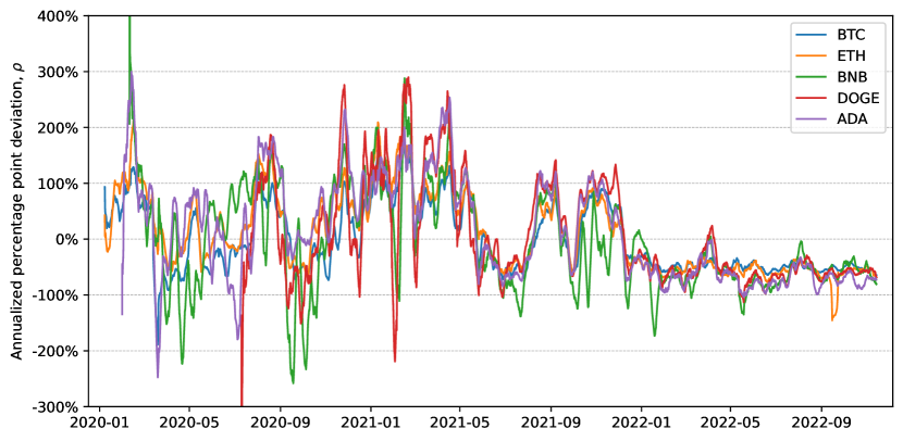
Figure 3: Deviations of perpetual futures from no-arbitrage benchmarks

This figure presents the 7-day moving averages of the annualized deviation of the perpetual futures-spot spread from the no-arbitrage benchmark for the five cryptocurrencies.

	$\rho$				$|\rho|$
Crypto	Mean	Median	Std	p-value	Mean	Median	Std	p-value
BTC	-0.02	-0.25	0.79	0.60	0.59	0.53	0.52	0.00
ETH	0.12	-0.09	0.89	0.13	0.67	0.56	0.61	0.00
BNB	-0.07	-0.18	1.32	0.70	0.94	0.73	0.93	0.00
DOGE	0.08	-0.18	1.62	0.28	1.01	0.72	1.27	0.00
ADA	0.12	-0.06	1.25	0.18	0.91	0.74	0.87	0.00

Table 4: Summary Statistics for Deviations from No-arbitrage Prices

The table below summarizes statistics for $\rho$ and $|\rho|$ across various crypto tokens. $p_{NW}$ corresponds to the Newey-West adjusted p-value, testing the null hypothesis that the mean $\rho$ (or $|\rho|$) is zero. The sample periods are shown in Table 2.

Table 4 reports summary statistics for $\rho$ and $|\rho|$ in our sample. As can be seen, the mean future-spot spread is modest, lying between $-2$ and 12 percentage points. The p-values show we cannot reject the hypothesis that the deviations are zero on average. Thus, on average our theoretical prices provide a useful benchmark. Around this benchmark, however, perpetual futures prices vary significantly from spot prices. The mean absolute deviation is about 60% to 100% per year across different cryptocurrency tokens. Figure 3 depicts the 7-day moving average of $\rho$ for each of the five examined cryptocurrencies. It reveals considerable comovement in futures-spot spreads across these cryptocurrencies, suggesting a common factor at play that drives the observed divergence. This observation is corroborated by Table LABEL:tab_corr, which demonstrates high correlations among futures-spot deviations across the different cryptocurrencies. This trend underscores the interconnectedness of cryptocurrency markets.

One hypothesis for this significant comovement in $\rho$ across various cryptocurrencies pertains to time-varying funding constraints encountered by arbitrageurs in the market (Brunnermeier and Pedersen, 2009; Garleanu and Pedersen, 2011). Because arbitrageurs often serve as marginal traders in all markets, their funding constraints are potentially reflected in the $\rho$ across all major cryptocurrency markets. Our theoretical and empirical analyses underscore the importance of measuring $\rho$. Doing so not only sheds light on potential market stress but also provides a gauge for the shadow costs associated with the trading and funding constraints arbitrageurs face.

Conversely, from the demand side, shared sentiment across various cryptocurrencies could also contribute to explaining the concurrent movement of $\rho$ across different markets. Our theoretical analysis suggests that arbitrageurs will only meet the market demand if the price deviation surpasses the combined trading and funding costs. As a result, the overall market sentiment in the futures market relative to the spot market becomes evident in the price difference between futures and spot prices. If the sentiment across different markets is influenced by a common factor, we would anticipate a significant comovement in the futures-spot spread. In Section 5, we delve deeper into explaining the futures-spot spread. Our results demonstrate that the past returns of each cryptocurrency serve as significant explanatory variables for the time-series variation in the spread.

Interestingly, the correlation between deviations and spot market returns is quite modest. Although spot market returns are highly correlated among themselves, in line with the strong market factor results from Liu et al. (2022), and no-arbitrage price deviations are highly correlated among themselves, it appears that different forces drive these distinct phenomena.

Furthermore, we find that after the year 2022, futures-spot spreads become smaller in magnitude and less volatile compared to earlier years. The 7-day moving average stays around -50% most of the time for the 5 cryptocurrencies while larger sways in earlier years are quite common. This suggests the market is becoming increasingly efficient. In terms of the sign of the deviation, which appears to stabilize at the negative region, two forces are potentially at play: (1) on the futures customer end, the relative demand in the futures market is weaker compared to the spot; (2) for arbitrageurs, because of the lack of infrastructure to short the cryptos in the spot market (high shorting costs), their funding constraints would be larger in the negative region. All these forces contribute to the stabilization of the futures spot deviation around $-50$ percentage points.

Last but not least, by design, $\rho$ is also highly correlated with the funding rate. The funding rate does not correlate perfectly with $\rho$ because in real-world implementations: (1) there is a clamp region, within which the funding rate is fixed at 0.01%; (2) the funding rate is calculated as a weighted average of futures-spot price deviations, with larger weight given to more recent observations; (3) in calculating the funding rate, Binance does not just consider the quote price, they also use an impact margin notional to consider price impact of the trade.

4.3 Random-maturity Arbitrage Strategy

We next provide a trading strategy motivated by our random-maturity arbitrage theory. Table 3 reports for different trading cost tiers, the bounds ($\rho_{l}$ and $\rho_{u}$) beyond which there exist random-maturity arbitrage opportunities. We consider a simple trading strategy: whenever $\rho$ enters the region outside the annualized round-trip trading costs in Table 3, we open the position. We close the position when $\rho$ first goes back to 0.

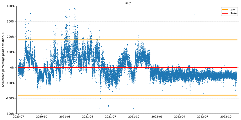
Figure 4: Random-maturity Arbitrage Strategy: Bitcoin, high trading costs

Futures-spot deviations and trading thresholds of the random-maturity arbitrage strategy we implement for BTC under high trading costs. Each blue dot in the figure represents the annualized deviation of futures from the spot $\rho=\kappa(f-s)-r$. The orange line is the open-position threshold and the red line is the close-position threshold.

Figure 4 provides an illustration of the trading strategy. When the deviation is beyond the orange lines, the strategy opens a trading position. The position is closed when the futures/spot deviation first hits the red line. We present trading thresholds across different trading costs for different currencies in Figure 10 in the appendix. Different trading strategies have the same close-position line which is equal to the risk-free rate while the open-position line adjusts to the level of trading costs.

Since our trading strategy is a threshold trading rule, to annualize Sharpe ratios we follow Lucca and Moench (2015), which considers a trading strategy that is only active on FOMC announcement dates. We first calculate the mean ($\mu$) and standard deviation ($\sigma$) of our trading strategy during the time it is active. Next, we scale $\mu/\sigma$ by the number of periods the strategy is active in a year:

$$SR=\frac{\mu}{\sigma}\sqrt{N_{a}}\ ,$$

where $\mu$ and $\sigma$ are average hourly returns and $N_{a}$ is the average number of hours the strategy is active in a year. We follow the same approach to annualize the returns and standard deviations: $\mu_{ann}=\mu N_{a}$, $\sigma_{ann}=\sigma\sqrt{N_{a}}$.

		Fee tiers
		No	Low	Medium	High
BTC	SR	3.94	2.50	2.31	1.92
	Return	17.89	11.21	10.13	8.15
	Volatility	4.54	4.48	4.39	4.25
	MaxDD	-4.24	-4.27	-4.34	-4.43
	$\alpha$	22.64	10.86	8.24	5.47
	$t_{\alpha}$	5.39	2.71	2.10	1.38
	Active %	100.00	84.93	43.87	22.32
	OtC time	15.80	63.90	95.97	113.38
ETH	SR	5.43	3.46	3.13	2.82
	Return	28.03	17.49	15.17	12.68
	Volatility	5.16	5.06	4.85	4.49
	MaxDD	-4.13	-4.21	-3.90	-3.94
	$\alpha$	45.55	23.09	18.33	14.42
	$t_{\alpha}$	7.56	4.25	3.69	3.15
	Active %	99.94	84.63	51.21	28.11
	OtC time	12.10	37.57	70.75	75.77
BNB	SR	12.49	8.07	6.41	5.44
	Return	62.38	38.40	29.14	23.43
	Volatility	4.99	4.76	4.55	4.31
	MaxDD	-1.12	-1.12	-1.10	-1.11
	$\alpha$	107.81	58.17	41.12	32.87
	$t_{\alpha}$	10.53	7.79	7.08	6.50
	Active %	99.97	89.25	66.67	39.94
	OtC time	7.87	14.65	22.20	24.07
DOGE	SR	12.61	8.34	5.96	4.42
	Return	112.09	70.88	49.74	35.82
	Volatility	8.89	8.49	8.35	8.10
	MaxDD	-8.56	-8.56	-8.56	-8.56
	$\alpha$	312.42	151.20	88.73	54.65
	$t_{\alpha}$	7.76	6.56	5.53	4.46
	Active %	99.85	90.35	68.52	36.90
	OtC time	5.56	8.50	11.21	11.26
ADA	SR	11.34	6.46	4.07	3.12
	Return	69.58	38.05	23.33	16.72
	Volatility	6.13	5.89	5.73	5.36
	MaxDD	-4.30	-4.26	-4.29	-4.34
	$\alpha$	120.52	52.28	27.52	18.11
	$t_{\alpha}$	14.56	10.22	6.55	4.59
	Active %	99.64	90.49	69.32	41.03
	OtC time	6.57	11.26	20.80	33.77

Table 5: Performance of Random-maturity Arbitrage Strategy

Performance under different trading cost tiers. The fees for spot (futures) are 2.25 (0.18) bps, 4.5 (0.72) bps, and 6.75 (1.44) bps for the low, medium, and high trading cost levels. Statistics reported are the annualized Sharpe ratio, return (%), volatility (%), max drawdown (%), alpha (%), t-stat of the alpha, proportion of time the strategy is active (%), and average open-to-close (OtC) position duration in hours.

Table 5 presents the strategy’s performance under different fee tiers. As trading costs decrease, the random-maturity arbitrage strategy engages in more active trading, leading to an increase in the SRs and a decrease in the average duration of open-to-close positions. The strategy also delivers highly significant alphas relative to the 3-factor model by Liu et al. (2022) and the 5-factor model by Cong et al. (2022a). Evidently, the strategy’s performance cannot be explained by previously suggested risk factors.

Table 6 zooms in and presents the trading performance of the strategy under high trading costs. We consider two cases: (1) unrestricted; (2) long-spot only. We consider the second case because, in earlier years of crypto derivatives, the infrastructure of shorting cryptocurrencies is not well-developed. We find that, as is implied by our theory, whenever the deviation between futures and spot is larger than the trading costs, performing a random-maturity arbitrage strategy would generate returns with high SR. After trading costs, the strategy generates a SR of 1.92 for BTC and much higher SRs for other cryptocurrencies.

		Unrestricted				Long-spot Only
		2020	2021	2022	All	2020	2021	2022	All
BTC	SR	2.26	2.39	1.23	1.92	1.98	2.28	0.55	1.75
	Return	8.28	14.80	0.26	8.15	6.43	13.96	0.10	7.16
	Volatility	3.67	6.18	0.21	4.25	3.25	6.12	0.18	4.10
	Active %	28.66	34.43	1.01	22.32	22.18	32.07	0.03	18.95
	N	8,616	8,760	7,536	24,912	8,616	8,760	7,536	24,912
ETH	SR	3.08	3.52	1.39	2.82	2.57	3.37	0.87	2.50
	Return	17.11	18.08	1.36	12.68	13.99	17.14	0.62	11.06
	Volatility	5.55	5.13	0.98	4.49	5.44	5.09	0.71	4.42
	Active %	37.80	34.91	9.12	28.11	34.40	34.54	0.09	24.07
	N	8,616	8,760	7,536	24,912	8,616	8,760	7,536	24,912
BNB	SR	6.04	6.60	2.61	5.44	4.45	5.00	0.68	3.94
	Return	31.26	33.13	4.04	23.43	15.32	21.94	0.16	12.99
	Volatility	5.17	5.02	1.55	4.31	3.44	4.39	0.24	3.29
	Active %	55.07	48.03	14.84	39.94	34.96	31.27	0.03	22.70
	N	7,815	8,760	7,536	24,111	7,815	8,760	7,536	24,111
DOGE	SR	4.90	5.93	1.93	4.42	2.64	5.05	1.11	3.10
	Return	59.81	53.51	1.94	35.82	31.16	36.34	0.29	22.02
	Volatility	12.19	9.02	1.00	8.10	11.80	7.19	0.26	7.11
	Active %	60.12	49.19	9.70	36.90	37.49	41.91	0.05	25.61
	N	4,190	8,760	7,536	20,486	4,190	8,760	7,536	20,486
ADA	SR	3.87	3.41	2.27	3.12	3.16	2.94	0.00	2.49
	Return	21.32	24.18	3.15	16.72	16.03	20.36	0.00	12.62
	Volatility	5.51	7.09	1.39	5.36	5.08	6.92	0.00	5.08
	Active %	47.61	42.18	32.66	41.03	36.41	39.53	0.00	26.27
	N	8,055	8,760	7,536	24,351	8,055	8,760	7,536	24,351

Table 6: Performance Over Time: High Trading Costs Tier

This table presents the Sharpe ratios, annualized returns (%), standard deviations (%), and active percentages (%) of the random-maturity arbitrage trading strategies for five different cryptocurrencies with high trading costs. We break down returns for each year and provide summary statistics across all time. The left panel shows the performance of the unrestricted trading strategy, where both long and short spot positions are allowed. The right panel shows the performance of the long-spot-only trading strategy, where shorting the spot is not allowed.

Table 6 also shows that as time goes by, the perpetual futures market seems to become more and more efficient. As we can see in 2022, the deviation of crypto price from the arbitrage-free bound is much less frequent compared to earlier years. But when the deviation happens, the resulting SR from the trade remains high.

Comparing the results with Du, Tepper, and Verdelhan (2018), we find that deviations in crypto perpetual futures are considerably larger in magnitude. As a result, gains from the arbitrage strategies we study are also larger. Even though the volatility of the trading strategy also scales up, the Sharpe ratios in the crypto space are still larger than those in the traditional foreign exchange market as reported in Du, Tepper, and Verdelhan (2018).

When a futures-spot gap opens up, gains from the trading strategy could potentially arise from two main sources: price convergence and funding rate payments. While industry publications usually emphasize the funding rate channel, we note that price convergence can generate quicker gains from arbitrage if dislocations are short-lived. To examine these two sources empirically, in Table 7 we provide a decomposition of the trading strategy’s performance into price convergence versus funding rate payment. We find that price convergence plays a dominant role in total trading returns, while funding rate payments have a more minor role, which seems to diminish over time.

		2020	2021	2022	All
BTC	Return	21.68	29.60	-0.05	17.89
	Price	14.00	14.29	2.11	10.51
	Funding	7.68	15.31	-2.16	7.39
ETH	Return	40.93	36.66	3.24	28.03
	Price	27.58	19.07	3.75	17.38
	Funding	13.35	17.59	-0.51	10.65
BNB	Return	82.48	76.29	25.36	62.38
	Price	66.70	60.37	20.00	49.80
	Funding	15.78	15.92	5.36	12.57
DOGE	Return	220.81	113.79	49.67	112.09
	Price	214.72	93.24	50.52	102.37
	Funding	6.09	20.55	-0.85	9.72
ADA	Return	90.81	66.73	50.19	69.58
	Price	77.17	49.51	49.05	58.52
	Funding	13.64	17.22	1.13	11.06

Table 7: Return Decomposition: Price Convergence vs Funding Rate Payment for Random-maturity Arbitrage Strategies

This table decomposes the portfolio return into the part due to price convergence and the part due to funding rate payment.

The success of the trading strategy supports the theory of random-maturity arbitrage. Whenever there is a deviation larger than the gap implied by the theory, betting on convergence tends to generate a positive payoff at some uncertain future time. Therefore, the convergence arbitrage trade generates high Sharpe ratios.

5 Explaining Futures-spot Deviations

From Figure 3, we observe a strong common comovement of the futures-spot deviation across all crypto assets. Our goal is to understand the fundamental forces driving this common factor. We consider two potential hypotheses: (1) the time-varying funding constraints of arbitrageurs, and (2) the time-varying relative demand from end-users for perpetual futures compared to the spot.

Both forces could potentially explain these patterns. Arbitrageurs will accommodate the relative demand from end-users only until the price deviation lies within the random-maturity no-arbitrage bound, which depends on arbitrageurs’ funding conditions. As arbitrageurs are likely the marginal investors in all cryptocurrency markets, their time-varying funding constraints may create common time-series variation in $\rho$ across different cryptocurrencies.

On the other hand, when the deviation lies within the no-arbitrage bound, variations in demand from the perpetual futures market compared to the spot market will influence the price deviation. It is plausible that relative demand has common factors across different cryptocurrencies. For instance, sentiment could drive their common variation, as perpetual futures allow for high leverage, which attracts overconfident, extrapolative, and sentiment-driven investors.

Determining which of the two factors better explains the observed price deviation is an empirical question. To shed light on this, we use past returns as a proxy for relative extrapolative demand in the perpetual futures market compared to the spot market. Past returns correlate with the demand from investors with extrapolative beliefs, who are more likely to trade in the perpetual futures market given the high leverage it provides. Therefore, past returns would correlate with the relative demand in the perpetual futures market compared to the spot.

For the time-varying funding constraint, we consider using crypto return volatility as a proxy, because, as in Adrian and Shin (2010), arbitrageurs likely face Value-at-Risk (VaR) type constraints, which are more likely to bind when market volatility is high.

Dependent Variable:	$\rho$
	BTC			ETH
Ret	0.28***		0.28***	0.20***		0.23***
	(7.79)		(7.74)	(3.87)		(4.83)
Vol		-0.02	-0.01		-0.01**	0.01
		(-1.60)	(-0.64)		(-1.99)	(1.58)
Const	-0.12**	0.30	-0.03	-0.06	0.36	-0.28*
	(-2.16)	(1.22)	(-0.16)	(-0.58)	(1.40)	(-1.67)
R2	0.55	0.03	0.56	0.47	0.03	0.49
N	1011	1011	1011	1011	1011	1011

Table 8: Regression of the futures-spot gap against explanatory variables

We present regression results of $\rho$ on the past four months’ annualized returns (Ret) and volatility (Vol) for Bitcoin and Ethereum. The left panel reports results for Bitcoin, and the right panel reports results for Ethereum. For each cryptocurrency, we consider three models: (1) regressing $\rho$ on past returns; (2) regressing $\rho$ on past volatility; and (3) regressing $\rho$ on both past returns and volatility. The observations are at a daily frequency. The sample period spans from January 30, 2020, to November 13, 2022, totaling 1,011 days. The table also reports the R-squared values for each regression model. We report HAC-robust t-statistics in parentheses. $*p<.1$, $**p<.05$, $***p<.01$

Table 8 presents the regression results of $\rho$ on past returns, volatility, and both for BTC and ETH. The regression coefficients on past returns are positive and highly significant. This suggests that when past returns are high, perpetual futures exhibit a more positive deviation against the spot. Mapping this back to our second hypothesis, when past returns are high, the demand for futures relative to the spot is also likely to be high. Consequently, even after arbitrageurs accommodate the demand outside of trading costs, the residual demand still manifests itself through the perpetual-spot deviation.

This observation on limits to arbitrage is related to Makarov and Schoar (2020) which finds that crypto price deviations across international exchanges tend to comove with one another. The driving force behind this comovement is investors’ buying pressure across various countries, with cross-country capital controls serving as the primary impediment to arbitrage capital. In the context of perpetual futures, end-user demand contributes to the comovement of different cryptocurrencies. The limits to arbitrage predominantly manifest in the form of trading frictions.

Liu and Tsyvinski (2021) document a significant time-series momentum pattern in the crypto market. Given that positive past returns lead to a positive gap between futures and spot prices, it is worth examining further whether the time-series momentum phenomenon is driven by margin trading and price pressure from the perpetual futures market. We leave this as an open question for future research.

We find that volatility does not significantly covary with the futures and spot deviation. This suggests that time-varying funding constraints of arbitrageurs do not drive the comovement in futures-spot deviations across different cryptocurrencies.

In summary, a prerequisite for the gap between futures and spot prices to occur is the existence of trading costs for arbitrageurs. Arbitrage trading will accommodate all the demand in the futures until the price deviation lies within a trading cost bound. Within the bound, the relative demand of futures compared to the spot will still manifest itself in the deviation of futures prices from the spot. Due to the comovement of the time-varying relative demand, we observe a significant common factor in crypto future-spot deviations.

6 Conclusion

Perpetual futures play an important role in today’s crypto markets and could potentially be adopted in non-crypto markets in the future. Understanding the fundamental mechanism of this financial derivative is a crucial first step for understanding speculation and hedging dynamics in this fast-evolving area. We provide a comprehensive analysis of the arbitrage and funding rate payment mechanisms that underpin perpetual futures.

In an ideal, frictionless world, we show that arbitrageurs would trade perpetual futures in such a way that a constant proportional relationship would hold between the futures price and the spot price. In the presence of trading costs, the deviation of the futures price from the spot would lie within a bound.

Motivated by the theory, we then empirically examine the comovement of the futures-spot spread across different cryptocurrencies and implement a theory-motivated arbitrage strategy. We find that this simple strategy yields substantial Sharpe ratios across various trading cost scenarios. The evidence supports our theoretical argument that perpetual futures-spot spreads exceeding trading costs represent a random-maturity arbitrage opportunity.

Finally, we provide an explanation for the common comovement in futures-spot spreads across different crypto-currencies: arbitrageurs can only accommodate market demand if the price deviation exceeds trading costs. As a result, the overall sentiment in the futures market relative to the spot market is reflected in the spread. Our empirical findings suggest that past return momentum can account for a significant portion of the time-series variation in the futures-spot spread.

Appendix

A. Additional figures and tables

Figure 5: Trading view of BTC perpetual futures on Binance

This figure presents the perpetual futures trading view on Binance. The key information includes the futures price (Mark), spot price (Index), real-time funding rate based on the rolling average of the past 8 hours’ observations, and countdown toward funding rate payment (Funding / Countdown) (illustrated with a red rectangle). In this example, futures are trading at a lower price than the spot. The funding rate is negative and is to be paid in 1 hour and 12 minutes.

Figure 6: Trading costs tiers for the spot market

This figure presents the trading costs tiers for the crypto spot market from Binance: https://www.binance.com/en/fee/trading. Our high, medium, and low trading cost specification corresponds to VIP 1, VIP 5, and VIP 8 tiers as illustrated with red rectangles in the picture. The 30-day trading volume requirements for VIP 1, 5, and 8 are 1 million, 150 million, and 2 billion respectively in the spot market. We consider the trading costs for makers as institutions typically trade maker orders. Binance offers a temporary discount for VIP 4-8 to have the same trading cost as VIP 9. We consider the non-discounted trading costs to make the comparison more reliable and fair.

Figure 7: Trading costs tiers for the perp market

This figure presents the trading costs tiers for the crypto perpetual market from Binance: https://www.binance.com/en/fee/trading. Our high, medium, and low trading cost specification corresponds to VIP 1, VIP 5, and VIP 8 tiers as illustrated with red rectangles in the picture. The 30-day trading volume requirements for VIP 1, 5, and 8 are 15 million, 1 billion, and 12.5 billion respectively in the perpetual market. We consider the trading costs for makers as institutions typically trade maker orders.

Figure 8: Ether annualized funding rate across exchanges

The figure presents the 7-day moving average annualized funding rate for Ether (ETH) across exchanges. The data is obtained from glassnode, an analytics platform. The data covers two major market turbulences: the COVID stock market crash from February to April 2020, and the FTX insolvency in November 2022. The FTX collapse led to significant negative funding rates on all solvent exchanges, thus the perpetual future prices were lower than the spot prices on the solvent exchanges. Vice versa on the insolvent FTX. The funding rates become more volatile after the event, indicating increased uncertainty for the market participants.

Figure 9: Annualized interest rate from Aave

This figure presents the daily supply and borrowing rate from Aave. We consider three stablecoins: USDT, USDC, and DAI. Each day, we take the average interest rate of the 3 crypto stablecoins to get the proxy for the risk-free funding rate of the arbitrageurs. The averaging removes the idiosyncratic noise in borrowing and supply in individual stablecoins. The sample period is from 2020-01-08 to 2022-11-13.

Figure 10: Trading Strategy Visualization: Random-maturity Arbitrage

This figure presents the random-maturity arbitrage strategy motivated by the theory. The orange, green and purple lines correspond to the open-position threshold under high, medium, and low trading costs. The red line represents the close-position threshold.

Figure 11: Trading Strategy Visualization: No Trading Costs

This figure presents the real-time trading thresholds under no trading costs. The orange line is the open-position threshold and the red line is the close-position threshold. The trading thresholds are determined based on the adjusted SR from the past 6 months.

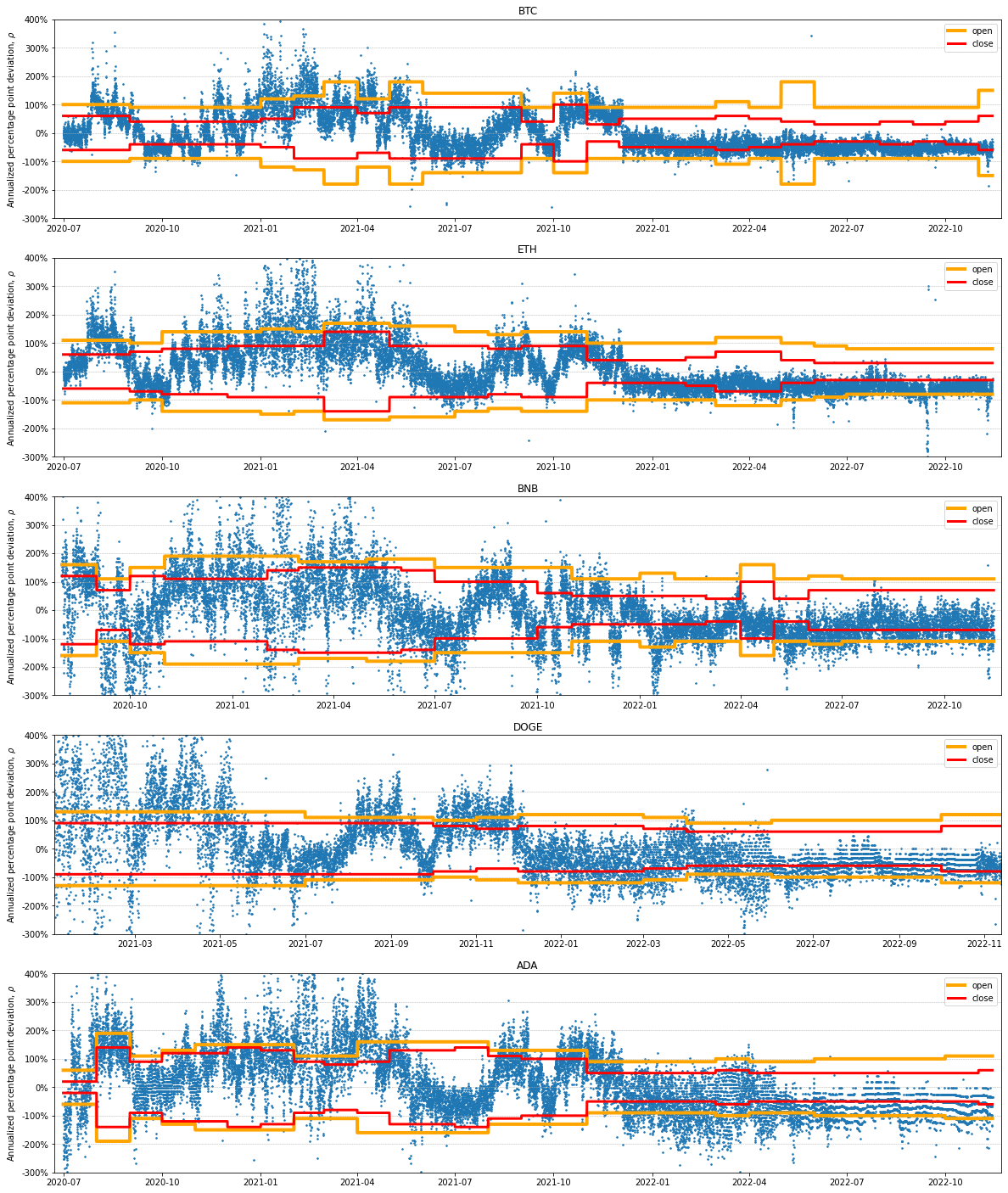
Figure 12: Trading Strategy Visualization: Low Trading Costs

This figure presents the real-time trading thresholds under low trading costs (2.25 bps for spot trading and 0.18 bp for futures trading). The orange line is the open-position threshold and the red line is the close-position threshold. The trading thresholds are determined based on the adjusted SR from the past 6 months.

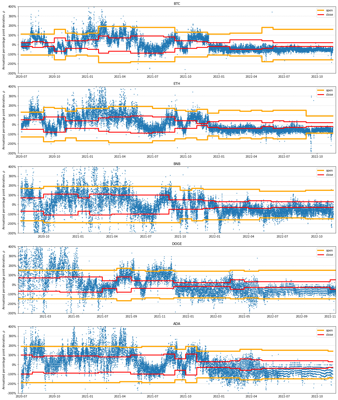
Figure 13: Trading Strategy Visualization: Medium Trading Costs

This figure presents the real-time trading thresholds under medium trading costs (4.5 bps for spot trading and 0.72 bp for futures trading). The orange line is the open-position threshold and the red line is the close-position threshold. The trading thresholds are determined based on the adjusted SR from the past 6 months.

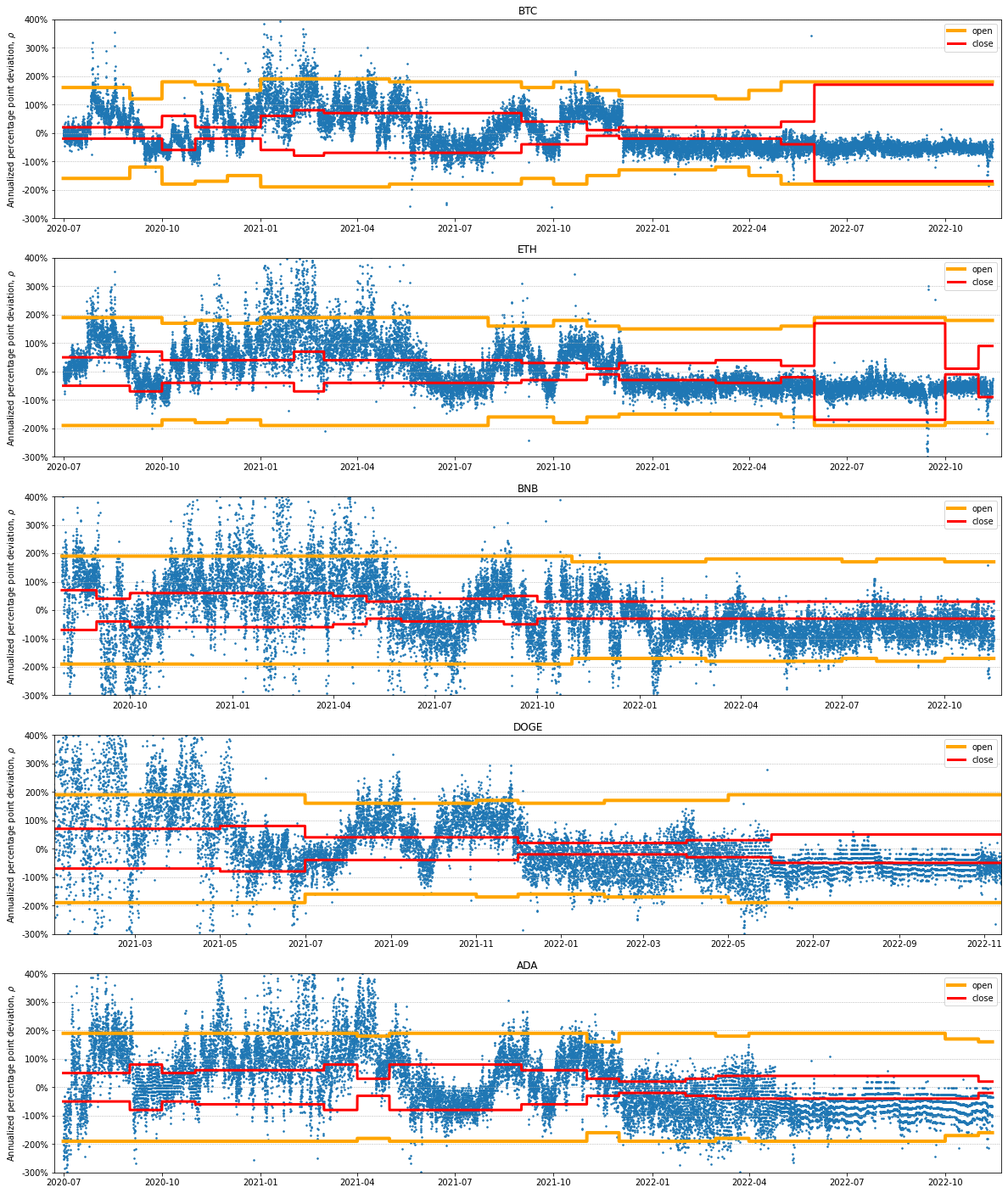
Figure 14: Trading Strategy Visualization: High Trading Costs

This figure presents the real-time trading thresholds under high trading costs (6.75 bps for spot trading and 1.44 bps for futures trading). The orange line is the open-position threshold and the red line is the close-position threshold. The trading thresholds are determined based on the adjusted SR from the past 6 months.

B. Data-driven Arbitrage Strategy

In the main text of our paper, we demonstrate the profitability of a simple theory-motivated trading strategy. The trading threshold can also be potentially further improved using a data-driven approach. In this part, we implement a data-driven two-threshold arbitrage trading strategy in the perpetual futures market. The strategy can be characterized with a tuple of two thresholds: $(u,l)$, where $u$ denotes the upper bar and $l$ denotes the lower bar, $u>l$. When $\rho>u$, we long the spot and short the futures. When $-l<\rho<l$, we close the position. When $\rho<-u$, we long the futures and short the spot. Figure 15 presents an illustration of the strategy for Bitcoin with the trading thresholds estimated using real-time data.

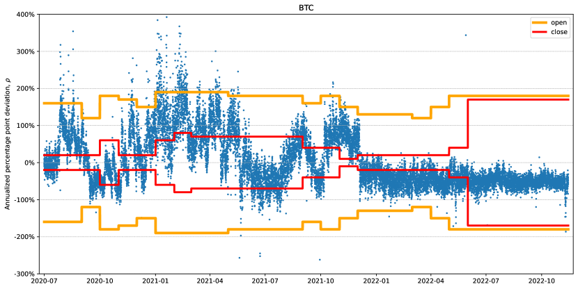
Figure 15: Data-driven strategy: Bitcoin, high trading costs

This figure presents real-time trading thresholds of the arbitrage strategy we implement for BTC under high trading costs. Each blue dot in the figure represents annualized deviation of futures from the spot $\rho=\kappa(f-s)-r$. The orange line is the open-position threshold and the red line is the close-position threshold.

To determine the optimal $(u,l)$, at the beginning of each month, we calculate the returns of the two-threshold trading strategy based on the past 6 months’ data on a grid of parameters. From Table 3, we find the theory implied bounds for price deviation across all trading costs specifications lie within $-200\%$ to $+200\%$. So we choose the grid as increasing from $0\%$ to $200\%$ with an incremental step of $10\%$ for $u$ and $l$ ($u\geq l$). In total, there are $210$ model specifications. We choose the model that delivers the highest Sharpe Ratio in the validation sample of the past 6 months.

Figure 15 presents the real-time trading thresholds of our arbitrage strategy for BTC under high trading costs. To mitigate the trading cost, the strategy automatically chooses a much lower close-position threshold compared to the open-position threshold. We also present the visualization of all trading strategies under different trading costs in appendix Figure 11 to 14. Under no-trading costs, the strategy chooses a low open-position threshold and the open- and close-position thresholds coincide with each other. Since there is no trading cost, the strategy no longer needs to wait for price convergence to avoid high turnover. On the contrary, with high trading costs, the strategy chooses a larger open-position threshold and a smaller close-position threshold. This reflects the automatic adjustment from the algorithm for trading costs and turnovers.

Table 9 presents the return statistics for this strategy under high trading costs over time. In the baseline ‘unrestricted’ strategy, we allow for both (1) longing the futures and shorting the spot and (2) shorting the futures and longing the spot while in the ‘long-spot only’ strategy, we only allow for shorting the futures and longing the spot. The reason we consider the ‘long-spot only’ strategy is the infrastructure for shorting the spot is not well-developed. So we want to examine the performance of the trading strategy in the presence of such limits to arbitrage.

		Unrestricted				Long-spot Only
		2020	2021	2022	All	2020	2021	2022	All
BTC	N	4,416	8,760	7,536	20,712	7,344	8,760	7,609	23,713
	Active %	26.11	18.06	0.29	13.31	30.27	52.45	0.03	28.76
	Return	5.78	8.51	0.13	4.88	6.24	15.21	0.10	7.58
	Volatility	3.74	3.26	0.19	2.74	3.47	6.50	0.18	4.40
	SR	1.55	2.61	0.70	1.78	1.80	2.34	0.54	1.72
ETH	N	4,416	8,760	7,536	20,712	5,880	8,760	7,609	22,249
	Active %	22.98	23.90	12.08	19.40	44.12	54.35	0.09	33.09
	Return	9.23	13.25	0.60	7.79	11.56	18.07	0.61	10.38
	Volatility	2.55	3.73	0.93	2.76	4.29	6.13	0.71	4.45
	SR	3.62	3.55	0.64	2.83	2.70	2.95	0.87	2.33
BNB	N	3,672	8,760	7,536	19,968	3,672	8,760	7,609	20,041
	Active %	41.04	32.32	10.51	25.69	57.30	48.11	1.10	31.94
	Return	24.61	25.33	3.33	16.89	12.23	20.07	0.10	11.05
	Volatility	4.24	4.23	1.32	3.44	3.77	4.80	0.30	3.57
	SR	5.80	5.99	2.52	4.91	3.24	4.18	0.33	3.10
DOGE	N		8,760	7,536	16,296		8,760	7,609	16,369
	Active %		41.66	6.62	25.45		54.26	1.22	29.60
	Return		47.57	0.98	26.02		32.74	0.08	17.56
	Volatility		7.93	0.87	5.85		7.39	0.40	5.42
	SR		6.00	1.14	4.45		4.43	0.21	3.24
ADA	N	4,416	8,760	7,536	20,712	4,416	8,760	7,609	20,785
	Active %	34.24	26.58	7.43	21.24	62.09	55.89	0.00	37.10
	Return	14.15	19.45	0.61	11.46	15.15	18.77	0.00	11.08
	Volatility	3.62	5.13	0.89	3.77	5.07	7.20	0.00	5.23
	SR	3.91	3.79	0.68	3.04	2.99	2.61	0.00	2.12

Table 9: Portfolio Performance: Data-driven strategy, High Trading Cost

This table presents the annual return, standard deviations, Sharpe ratios of the two-threshold trading strategies for the 5 different cryptocurrencies with high trading costs. We also report the proportion of time the trading strategy has an open position. We break down returns into each year and also provide summary stat across all time. The left panel shows the performance of the unrestricted trading strategy where both long and short spot is allowed. The right panel shows the performance of the long-spot-only trading strategy where shorting the spot is not allowed.

We find the arbitrage trading strategy has a high Sharpe ratio under high trading costs. The annualized Sharpe ratio for Bitcoin is 1.78 in our sample. They are even higher for other cryptos. The high Sharpe ratio of the trading strategy corroborates our theoretical results that when the price deviation is large enough, the trading would be a random-maturity arbitrage opportunity.

In the year 2022, the deviation between the futures and the spot becomes smaller and less volatile. There seems to be a structural break. We indeed find the trading strategy takes less active positions and significantly lower annualized returns. However, when there is a large enough deviation, the strategy can still generate sizeable Sharpe ratios in trading.

The conclusion and results remain similar if we consider ‘long-spot only’ trading strategies where only shorting the futures and longing the spot is allowed. Considering this one-sided trade slightly lowers the Sharpe ratio but the algorithm automatically adjusts by increasing the proportion of times being active. The resulting annualized returns increase. In the year 2022, since most of the time, the futures price is below the spot and we don’t allow longing the futures and shorting the spot trade, the proportion of time the strategy is active is very low.

		Trading costs
		No	Low	Medium	High
BTC	Active %	23.20	20.79	16.29	13.31
	Return	15.98	7.42	6.02	4.88
	Volatility	2.38	2.63	2.61	2.74
	SR	6.72	2.82	2.31	1.78
ETH	Active %	32.34	25.85	20.84	19.40
	Return	23.48	11.80	9.41	7.79
	Volatility	2.27	2.27	2.69	2.76
	SR	10.32	5.20	3.50	2.83
BNB	Active %	37.76	30.90	25.52	25.69
	Return	54.50	30.40	22.07	16.89
	Volatility	3.26	3.02	3.12	3.44
	SR	16.72	10.07	7.07	4.91
DOGE	Active %	36.62	39.81	32.46	25.45
	Return	72.95	46.87	34.45	26.02
	Volatility	5.65	5.60	5.81	5.85
	SR	12.90	8.37	5.92	4.45
ADA	Active %	40.00	43.22	24.38	21.24
	Return	53.06	29.63	16.53	11.46
	Volatility	3.22	3.33	3.26	3.77
	SR	16.47	8.90	5.07	3.04

Table 10: Data-driven strategy: Portfolio Performance under Different Trading Costs

This table presents the portfolio performance under different trading cost specifications. The fee for spot is 0, 1.5 bps, 3.75 bps, and 5.25 bps for the 4 trading costs specifications. The fee for the futures are 0, 0, 0.54 bp, 1.08 bps for the 4 trading costs specifications.

Table 10 further reports the performance of the trading strategy under different trading costs specifications laid out in Table 2. The results from Table 9 correspond to the last column in Table 10. As trading costs increase, our trading strategy dynamically adjusts by lowering the proportion of time being active. The annualized return decreases and annualized standard deviation are of similar magnitude across different trading costs. As a result, SR decreases as trading costs increase. Under no trading cost, we see a Sharpe ratio of 6.72 for BTC and Sharpe ratios above 10 for all other cryptos. This also confirms our theoretical results that when there is no trading cost, any deviation of perpetual price from the no-arbitrage benchmark would be a random-maturity arbitrage opportunity.

Comparing Table 10 with Table 5, we find under low and no trading costs, the potential incremental benefits from using a data-driven two-threshold trading rule are much larger compared to higher trading costs. The intuition can be easily illustrated by comparing the empirical real-time trading thresholds in the theory-motivated strategy and the data-driven strategy under low trading costs (Figure 10 and Figure 11). With persistent $\rho$ the data-driven approach can find the optimal close-position threshold corresponding to the level of $\rho$ while the theory-motivated one is too conservative in setting a close-position threshold equal to 0.

There are two sources of trading profit for our trading strategy: (1) the price convergence; (2) the funding rate payment. In Table 11, we decompose the return to our trading strategy without trading cost into the two sources. We find across different cryptos, the return from price convergence accounts for a larger proportion of the total profit. For BTC, the price convergence accounts for more than $2/3$ of the profits, and for ETH, it accounts for about $3/4$. Additionally, the decomposition for the year 2022 generates different patterns, the return due to funding rate plays a much smaller role across different cryptos. This is because the deviation from perpetual to spot is much smaller during the year. The results suggest when more sophisticated arbitrageurs enter the market, the large deviation of perpetual from the spot would be more of an off-equilibrium outcome. As a result, the funding rate payment will also be small.

		2020	2021	2022	All
BTC	Return	17.70	25.69	3.69	15.98
	Price	11.77	16.10	3.58	10.62
	Funding	5.93	9.59	0.11	5.36
ETH	Return	22.51	30.99	15.31	23.48
	Price	14.22	21.86	14.36	17.50
	Funding	8.29	9.13	0.95	5.98
BNB	Return	74.35	64.93	32.71	54.50
	Price	61.16	56.63	28.70	46.92
	Funding	13.19	8.29	4.01	7.58
DOGE	Return		96.17	45.95	72.95
	Price		82.50	45.58	65.43
	Funding		13.68	0.36	7.52
ADA	Return	44.24	56.21	54.57	53.06
	Price	31.81	45.69	53.12	45.44
	Funding	12.43	10.52	1.44	7.62

Table 11: Data-driven strategy: Price Convergence vs Funding Rate Payment

This table decomposes the portfolio return into the part due to price convergence and the part due to funding rate payment.

In all, our analysis of the trading strategy demonstrates the profitability of perpetual-spot arbitrage trade. The deviation of the futures to spot can also serve as an important measure for the frictions, trading costs, and limits to arbitrage in the market.

References

- Adams et al. (2021) Adams, Hayden, Noah Zinsmeister, Moody Salem, River Keefer, and Dan Robinson, 2021, Uniswap v3 core, Whitepaper .
- Adrian and Shin (2010) Adrian, Tobias, and Hyun Song Shin, 2010, Liquidity and leverage, Journal of financial intermediation 19, 418–437.
- Alexander et al. (2020) Alexander, Carol, Jaehyuk Choi, Heungju Park, and Sungbin Sohn, 2020, Bitmex bitcoin derivatives: Price discovery, informational efficiency, and hedging effectiveness, Journal of Futures Markets 40, 23–43.
- Amiram et al. (2021) Amiram, Dan, Evgeny Lyandres, and Daniel Rabetti, 2021, Cooking the order books: Information manipulation and competition among crypto exchanges, SSRN Electronic Journal .
- Angeris et al. (2022) Angeris, Guillermo, Tarun Chitra, Alex Evans, and Matthew Lorig, 2022, A primer on perpetuals, arXiv .
- Brunnermeier and Pedersen (2009) Brunnermeier, Markus K, and Lasse Heje Pedersen, 2009, Market liquidity and funding liquidity, The review of financial studies 22, 2201–2238.
- Cochrane (2009) Cochrane, John, 2009, Asset pricing: Revised edition (Princeton university press).
- Cong et al. (2022a) Cong, Lin William, Zhiheng He, and Ke Tang, 2022a, Staking, token pricing, and crypto carry, SSRN Electronic Journal .
- Cong et al. (2022b) Cong, Lin William, George Andrew Karolyi, Ke Tang, and Weiyi Zhao, 2022b, Value premium, network adoption, and factor pricing of crypto assets, SSRN Electronic Journal .
- Cong et al. (2022c) Cong, Lin William, Xi Li, Ke Tang, and Yang Yang, 2022c, Crypto wash trading, Technical report, National Bureau of Economic Research.
- De Blasis and Webb (2022) De Blasis, Riccardo, and Alexander Webb, 2022, Arbitrage, contract design, and market structure in bitcoin futures markets, Journal of Futures Markets 42, 492–524.
- Du et al. (2018) Du, Wenxin, Alexander Tepper, and Adrien Verdelhan, 2018, Deviations from Covered Interest Rate Parity, Journal of Finance 73, 915–957.
- Duffie (2010) Duffie, Darrell, 2010, Presidential address: Asset price dynamics with slow-moving capital, The Journal of finance 65, 1237–1267.
- Ferko et al. (2022) Ferko, Alex, Amani Moin, Esen Onur, and Michael Penick, 2022, Who trades bitcoin futures and why?, Global Finance Journal 100778.
- Garleanu and Pedersen (2011) Garleanu, Nicolae, and Lasse Heje Pedersen, 2011, Margin-based asset pricing and deviations from the law of one price, The Review of Financial Studies 24, 1980–2022.
- Gromb and Vayanos (2018) Gromb, Denis, and Dimitri Vayanos, 2018, The dynamics of financially constrained arbitrage, The Journal of Finance 73, 1713–1750.
- Hertzog et al. (2017) Hertzog, Eyal, Guy Benartzi, Galia Benartzi, and Omri Ross, 2017, Bancor protocol, continuous liquidity for cryptographic tokens through their smart contracts, Whitepaper .
- Koijen et al. (2018) Koijen, Ralph SJ, Tobias J Moskowitz, Lasse Heje Pedersen, and Evert B Vrugt, 2018, Carry, Journal of Financial Economics 127, 197–225.
- Liu and Tsyvinski (2021) Liu, Yukun, and Aleh Tsyvinski, 2021, Risks and returns of cryptocurrency, The Review of Financial Studies 34, 2689–2727.
- Liu et al. (2022) Liu, Yukun, Aleh Tsyvinski, and Xi Wu, 2022, Common risk factors in cryptocurrency, The Journal of Finance 77, 1133–1177.
- Lucca and Moench (2015) Lucca, David O, and Emanuel Moench, 2015, The pre-fomc announcement drift, The Journal of finance 70, 329–371.
- Makarov and Schoar (2020) Makarov, Igor, and Antoinette Schoar, 2020, Trading and arbitrage in cryptocurrency markets, Journal of Financial Economics 135, 293–319.
- Pedersen (2019) Pedersen, Lasse Heje, 2019, Efficiently inefficient: how smart money invests and market prices are determined (Princeton University Press).
- Schmeling et al. (2022) Schmeling, Maik, Andreas Schrimpf, and Karamfil Todorov, 2022, Crypto carry, SSRN Electronic Journal .
- Shiller (1993) Shiller, Robert J, 1993, Measuring asset values for cash settlement in derivative markets: hedonic repeated measures indices and perpetual futures, The Journal of Finance 48, 911–931.
- Streltsov and Ruan (2022) Streltsov, Artem, and Qihong Ruan, 2022, Perpetual price discovery and crypto market quality, SSRN Electronic Journal .