Sums of Two Squares Visualized

Abstract

We provide a geometric interpretation of Brillhart’s celebrated algorithm for expressing a prime $p\equiv 1\pmod{4}$ as the sum of two squares.

1 Introduction

On Christmas Day 1640, Pierre de Fermat stated his famous “two-square” theorem in a letter to Marin Mersenne. This theorem, which was first stated by Girard in 1625, and first proved by Euler in 1749, states that an odd prime $p$ is the sum of two squares if (and only if) $p\equiv 1\pmod{4}$. Among the many admirers of the theorem was G.H. Hardy, who wrote in A Mathematician’s Apology that the theorem is one of the finest of arithmetic, and also that “there is no proof within the comprehension of anybody but a fairly expert mathematician.”

Perhaps Hardy meant to encourage his younger readers, and flatter his older ones! In any case, his famous textbook with E. M. Wright An Introduction to the Theory of Numbers contains a neat geometrical proof of the two-square theorem, due to J.H. Grace [4]. Grace’s proof can be summarized as follows. First, we solve the congruence $u^{2}+1\equiv 0\pmod{p}$. (No major expertise required here: writing $p=4k+1$, a short argument using Wilson’s theorem shows that $u=(2k)!$ is a solution. The proof is due to Lagrange.) Next consider the integer lattice $L$ given by

$$L=\{(x,y)\in\mathbb{Z}^{2}:x\equiv uy\pmod{p}\}.$$ (1)

$L$ is a lattice containing a proportion $1/p$ of integer points; more precisely, the area of any fundamental parallelogram of the lattice is $p$. But $L$ is also a square lattice, since if $P=(g,h)$ is a point of $L$ closest to the origin $O$, then $g\equiv uh\pmod{p}$, so that $ug\equiv-h\pmod{p}$, and so $(-h,g)\in L$ too. These two facts together imply that the area $g^{2}+h^{2}$ of the square on side $OP$ is $p$, proving the theorem.

All well and good. But is there a fast algorithm for finding $g$ and $h$? Indeed there is. In 1972, John Brillhart [2], building on earlier work of Legendre, Serret and Hermite, proposed the following method, starting with $p$ and the number $u$ defined above. If $p=u^{2}+1$, stop. Otherwise, simply apply the Euclidean algorithm to $p$ and $u$, and stop when the first remainder $r$ satisfies $r<\sqrt{p}$. If the next remainder is $r^{\prime}$, then $(g,h)=(r,r^{\prime})$. (The fly in the ointment is that we first need to find $u$. Lagrange’s formula $u=(2k)!$ is computationally inefficient, but Shiu [5] provides a non-deterministic algorithm with a short expected running time; the key is to first find a quadratic non-residue modulo $p$, and then repeatedly square it.)

An example will serve to illustrate the method. Let $p=73$, and solve $u^{2}+1\equiv 0\pmod{p}$ to get $u=\pm 27$. Taking $u=27$, the Euclidean algorithm now yields:

$$73 =2\cdot 27+19$$

$$27 =1\cdot 19+{\bf 8}$$

$$19 =2\cdot 8+{\bf 3}$$

and, lo and behold, $8^{2}+3^{2}=73$.

Magic? Maybe. Certainly, Brillhart’s proof of his algorithm’s correctness is somewhat mysterious, even after simplification by Wagon [6]. Shiu [5] proves it using properties of continuants. But a closer look at Grace’s proof reveals that Brillhart’s algorithm has a secret geometric twin: Lagrange’s algorithm.

2 Lattice reduction

Two integer vectors in $\mathbb{R}^{2}$, such as ${\bf b_{1}}=(3,1)^{\sf T}$ and ${\bf b_{2}}=(5,3)^{\sf T}$, generate a lattice $L$ in the plane, consisting of all vectors of the form $m{\bf b_{1}}+n{\bf b_{2}}$, where $m$ and $n$ are integers. Noting that $||{\bf b_{1}}||=\sqrt{10}$ and $||{\bf b_{2}}||=\sqrt{34}$, we might wonder if there is a better way of generating the same lattice. What do we mean by better? One answer is that we should try to minimize $||{\bf b_{1}}||$ and $||{\bf b_{2}}||$. Equivalently, we need to find the two points of $L$ closest to the origin $O$. It turns out that there is a simple way to do this, which was discovered independently by Lagrange (first) and Gauss (second). We will call it Lagrange’s algorithm. It is similar to the Gram-Schmidt process, but more complicated, since we are only allowed to adjust vectors by integer multiples of other vectors, because we need to stay inside the lattice $L$. Indeed, given any two linearly independent vectors in $\mathbb{R}^{2}$, the Gram-Schmidt process terminates after one step, while Lagrange’s algorithm will terminate, but, depending on the initial two vectors, could take arbitrarily many steps to do so.

Figure 1 illustrates how Lagrange’s algorithm works. We start with ${\bf b_{1}}$ (shorter) and ${\bf b_{2}}$ (longer, or, for the first step only, at least as long as ${\bf b_{1}}$). Next, we reduce the longer vector ${\bf b_{2}}$ by adding or subtracting multiples of the shorter vector ${\bf b_{1}}$, to get ${\bf b_{3}}={\bf b_{2}}-q{\bf b_{1}}$, where the integer $q$ is chosen to make $||{\bf b_{3}}||$ as short as possible. For ${\bf b_{1}}=(3,1)^{\sf T}$ and ${\bf b_{2}}=(5,3)^{\sf T}$, illustrated on the left of Figure 1, we get ${\bf b_{3}}=(-1,1)^{\sf T}$. Notice that $||{\bf b_{3}}||=\sqrt{2}$, so that ${\bf b_{1}}$ and ${\bf b_{2}}$ have exchanged places; the shortened version ${\bf b_{3}}$ of ${\bf b_{2}}$ is now strictly shorter than ${\bf b_{1}}$. This means that we should exchange the vectors, setting ${\bf b^{\prime}_{1}=b_{3}}$ and ${\bf b^{\prime}_{2}=b_{1}}$, and repeat. The second step of the algorithm is shown on the right of Figure 1. The new shortened vector is ${\bf b^{\prime}_{3}}=(2,2)^{\sf T}$, of length $\sqrt{8}$.

Figure 1: Two steps of Lagrange’s algorithm

But now there is a problem. This time, ${\bf b^{\prime}_{1}}$ and ${\bf b^{\prime}_{2}}$ have not exchanged places; the adjusted longer vector ${\bf b^{\prime}_{3}}$ is still longer than (or, in general, at least as long as) the shorter vector ${\bf b^{\prime}_{1}}$. The resulting basis, consisting of ${\bf b^{\prime\prime}_{1}=b^{\prime}_{1}}$ and ${\bf b^{\prime\prime}_{2}=b^{\prime}_{3}}$, is said to be Lagrange-reduced. This means that ${\bf b^{\prime\prime}_{1}}$ and ${\bf b^{\prime\prime}_{2}}$ satisfy

$$||{\bf b^{\prime\prime}_{1}}||\leq||{\bf b^{\prime\prime}_{2}}||\leq||{\bf b^{\prime\prime}_{2}-qb^{\prime\prime}_{1}}||$$

for all integers $q$. Lagrange’s algorithm terminates here. (In this example, the final basis is orthogonal, but in general it need not be.)

It is nontrivial that Lagrange’s algorithm does yield two basis vectors of minimal length, which are thus the closest and second-closest lattice points to the origin. The proof, left as an exercise in [3], and presented in full in [1], is about half a page long.

Lagrange’s algorithm is very reminiscent of the Euclidean algorithm, with two quantities leapfrogging each other in a race to the bottom. Consequently, it may now be clear to the reader that (as stated without proof in [7]) Brillhart’s algorithm is just Lagrange’s algorithm applied to Grace’s lattice (1), starting with ${\bf b_{1}}=(u,1)^{\sf T}$ and ${\bf b_{2}}=(p,0)^{\sf T}$. But the algorithms are in fact different, even for the case $p=73,u=27$ considered earlier. Before proceeding, the reader is encouraged to run the two algorithms for this special case.

3 The plot thickens

The basic connection between Lagrange’s algorithm and Brillhart’s is that, at least initially, the $x$-components of the sequence of vectors produced by Lagrange’s algorithm (applied to $(p,0)^{\sf T}$ and $(u,1)^{\sf T}$) are the remainders in the Euclidean algorithm (applied to $p$ and $u$). Indeed, if the $y$-components are small, we can neglect them, so that Lagrange’s algorithm is approximated by its one-dimensional version, which is precisely the Euclidean algorithm.

Or is it? Figure 2 shows the result of applying Lagrange’s algorithm to the vectors $(73,0)^{\sf T}$ and $(27,1)^{\sf T}$. It does indeed produce (essentially) the same answer as Brillhart’s. But look at the $x$-components. Instead of the expected sequence $73,27,19,8,3$, we see $73,27,3,-8$. The number 19 is absent entirely, and 8 and 3 are replaced by 3 and -8. So the two algorithms are different. They are also different when, for example, $p=277$.

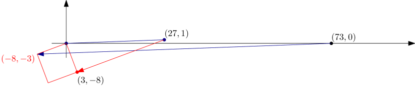
Figure 2: Lagrange’s algorithm

The resolution to this paradox is that the one dimensional version of Lagrange’s algorithm is not the ordinary version of Euclidean algorithm with non-negative remainders. Instead, it is the version where the remainders are chosen to minimize their absolute values. So the obvious way to connect the algorithms is to modify Brillhart’s algorithm to use this version of Euclid’s algorithm instead. Then it will run even faster.

The catch is that the fast Brillhart algorithm doesn’t work, in the sense that it doesn’t produce the required goods! Taking $p=277$ and $u=60$, we get

$$277 =5\cdot 60-23$$

$$60 =3\cdot 23-9$$

$$23 =3\cdot 9-4$$

which misses the solution $9^{2}+14^{2}=277$ entirely.

Fortunately, there is another possibility. We can modify Lagrange’s algorithm instead. And the obvious way to do this is to insist that every vector it generates has positive $x$-component. Figure 3 shows the result of applying this modification of Lagrange’s algorithm with initial vectors $(73,0)^{\sf T}$ and $(27,1)^{\sf T}$ This time, the sequence of $x$-components does match the (positive) remainders. And, finally, it is not hard to modify the proof from [1] to show that the modified Lagrange algorithm also terminates with a Lagrange-reduced basis, at least for the lattices under consideration.

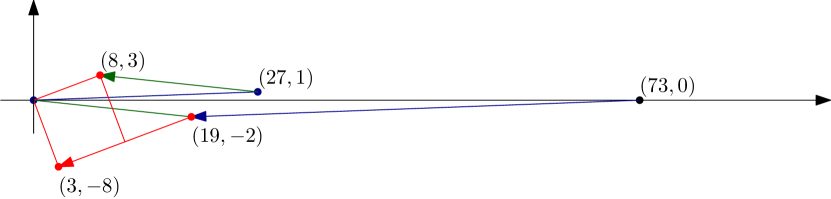
Figure 3: Lagrange’s algorithm, restricted to $x>0$

4 A calculation

There is one final hurdle to clear. These approximations are only valid when the $y$-components of the relevant vectors are small. Once they start growing, the shortest vector ${\bf b_{3}}$ from (the modified) Lagrange algorithm might not be the one with the smallest $x$-component. We will show that, in fact, these vectors coincide, until both algorithms terminate with the same result.

To do this, it will be convenient to change notation slightly, and to work with points in $\mathbb{R}^{2}$, instead of their position vectors. Let’s introduce the notation by restating both algorithms.

Ingredients: $p\equiv 1\pmod{4}$ is a prime, and $u$ satisfies $u^{2}\equiv-1\pmod{p}$ with $1\leq u<p/2$.

Initialization: We start with ${\bf x}_{0}=(x_{0},y_{0})={\bf x}^{\prime}_{0}=(p,0)$ and ${\bf x}_{1}=(x_{1},y_{1})={\bf x}^{\prime}_{1}=(u,1)$.

Brillhart’s Algorithm [2]: For $i=1,2,\ldots$, we write $x_{i-1}=q_{i}x_{i}+r_{i}$ with $0\leq r_{i}<x_{i}$, and set

$${\bf x}_{i+1}={\bf x}_{i-1}-q_{i}{\bf x}_{i}=(x_{i-1}-q_{i}x_{i},y_{i-1}-q_{i}y_{i})=(r_{i},y_{i-1}-q_{i}y_{i}).$$

Note that here we have extended Brillhart’s algorithm to produce points in $\mathbb{R}^{2}$, and we have also extended it to run until Euclid’s algorithm terminates. The sequence $(x_{i})$ is just the sequence of remainders $(r_{i})$ from the Euclidean algorithm applied to $p$ and $u$, while the sequence $(y_{i})$ is also related to the Euclidean algorithm: we have $r_{i}=s_{i}p+y_{i}u$ for another sequence $(s_{i})$ (see [6]).

For example, with $p=193$ we have $u=81$, and successive ${\bf x}_{i}$ are given by

$$(193,0),(81,1),(31,-2),(19,5),(12,-7),(7,12),(5,-19),(2,31),(1,-81),(0,193).$$

The symmetry is related to the fact that $u^{2}\equiv-1\pmod{p}$; we will derive it as a consequence of the arguments below.

The Modified Lagrange (ML) Algorithm: For $i=1,2,\ldots$, as long as $||{\bf x^{\prime}}_{i}||\leq||{\bf x^{\prime}}_{i-1}||$, write

$$q^{\prime}_{i}=\left\lfloor\frac{{\bf x^{\prime}}_{i}\cdot{\bf x^{\prime}}_{i-1}}{||{\bf x^{\prime}}_{i}||^{2}}\right\rfloor,$$

and set

$${\bf x^{\prime}}_{i+1}={\bf x^{\prime}}_{i-1}-q^{\prime}_{i}{\bf x^{\prime}}_{i}.$$

Our aim is to show that, with the above choices of $p$ and $u$, the two sequences do indeed coincide, until the ML algorithm terminates at ${\bf x}_{t}=(x_{t},y_{t})$. (In the example above, $(x_{t},y_{t})=(7,12)$.) In other words, we need to show that $q_{i}=q^{\prime}_{i}$, until the ML algorithm terminates.

We recall some details from earlier. First, the integer lattice $L$ given by

$$L=\{(x,y)\in\mathbb{Z}^{2}:x\equiv uy\pmod{p}\}$$

is a square lattice with determinant $p$, so that, for all $(x,y)\in L$, we have $p\mid(x^{2}+y^{2})$, and, if $(x,y)\in L$ is a point closest to the origin, then $p=x^{2}+y^{2}$. Consequently, if Lagrange’s algorithm terminates at ${\bf x}_{t}=(x_{t},y_{t})$, then $p=||{\bf x}_{t}||^{2}=x_{t}^{2}+y_{t}^{2}$.

We now observe that each of the points ${\bf x}_{i}$ (and ${\bf x}^{\prime}_{i}$) lies on $L$. Consequently, for all $i\geq 1$,

$$p\mid(x_{i}^{2}+y_{i}^{2}).$$ (2)

Moreover, it is easy to see by induction that, for all $i\geq 1$,

$$x_{i-1}y_{i}-x_{i}y_{i-1}=p,$$ (3)

and so

$$(x_{i-1}x_{i}+y_{i-1}y_{i})^{2} =(x_{i-1}^{2}+y_{i-1}^{2})(x_{i}^{2}+y_{i}^{2})-(x_{i-1}y_{i}-x_{i}y_{i-1})^{2}$$

$$=(x_{i-1}^{2}+y_{i-1}^{2})(x_{i}^{2}+y_{i}^{2})-p^{2},$$

so that

$$p\mid(x_{i-1}x_{i}+y_{i-1}y_{i}).$$ (4)

We can use these properties to establish the symmetry observed earlier. Suppose the (extended) Brillhart algorithm terminates at $(x_{T},y_{T})$. Then, since the $x_{i}$ are just the reminders $r_{i}$ in the Euclidean algorithm, we must have $x_{T}=0$ and $x_{T-1}=1$. By (2) we get $y_{i}=p$, and, since $(x_{T-1},y_{T-1})\in L$, we then get $y_{i-1}=-u$. We can now establish the required symmetry by induction (see also [6]).

Now, it is easy to show, by induction, that the $y_{i}$ alternate in sign, and that the sequence $|y_{i}|$ is increasing. From the remarks above, the sequence $(|y_{i}|)$ is just the sequence $(x_{i})$ in reverse order. Consequently, we can stop iterating once $x_{i}\leq|y_{i}|$. Thus, in the following, we will assume that $x_{i}>|y_{i}|$.

Claim: For all $i\geq 1$, $q_{i}=q^{\prime}_{i}$.

Proof: We use induction on $i$. The induction starts. For the induction step, we need to show that

$$q_{i}:=\left\lfloor\frac{x_{i-1}}{x_{i}}\right\rfloor=\left\lfloor\frac{x_{i-1}x_{i}+y_{i-1}y_{i}}{x^{2}_{i}+y_{i}^{2}}\right\rfloor=:q^{\prime}_{i}.$$

For simplicity of notation, write $a,b,c,d$ for $x_{i-1},y_{i-1},x_{i},y_{i}$ respectively. Then we need that

$$\left\lfloor\frac{a}{c}\right\rfloor=\left\lfloor\frac{ac+bd}{c^{2}+d^{2}}\right\rfloor.$$

Suppose first that $q^{\prime}_{i}<q_{i}$. Then there is an integer $m$ with

$$\frac{ac+bd}{c^{2}+d^{2}}<m\leq\frac{a}{c}.$$ (5)

Now, from the above, we know there are integers $K$ and $L$

$$ac+bd=pK{\rm\ and\ }c^{2}+d^{2}=pL.$$

Multiplying (4) by $c(c^{2}+d^{2})$, and noting that $y_{i}=d<c=x_{i}$, we get

$$cpK =c(ac+bd)<mc(c^{2}+d^{2})$$

$$=mcpL\leq a(c^{2}+d^{2})$$

$$=c(ac+bd)+d(ad-bc)$$

$$=cpK+dp<cpK+cp$$

$$=cp(K+1),$$

so that, dividing both sides by $cp$, we have

$$K<mL<K+1,$$

a contradiction.

The case where $q_{i}<q^{\prime}_{i}$ is handled similarly; this corresponds to the case $y_{i}=d<0$.

5 Exercise

There is one remaining mystery. We’ve shown that Brillhart’s algorithm is equivalent to the modified Lagrange algorithm. The original Lagrange algorithm, meanwhile, corresponds to the modified Brillhart algorithm, but the two can’t quite be equivalent, since the former works and the latter doesn’t. Explain why!

6 Acknowledgment

Both authors are extremely grateful to the second author’s teacher and mentor, Peter Shiu, whose paper [5] was the inspiration for this project, and whose subsequent communication and feedback has been indispensable.

References

- [1] C. Bright, Algorithms for lattice bass reduction , available at: https://cs.uwaterloo.ca/ cbright/reports/latticealgs.pdf.
- [2] J. Brillhart, Note on representing a prime as a sum of two squares, Math. Comp. 26 (1972), 1011–1013.
- [3] S. Galbraith, Mathematics and Public Key Cryptography, Cambridge University Press, 2012.
- [4] J. Grace, The four square theorem, J. Lond. Math. Soc. 2 (1927), 3–8.
- [5] P. Shiu, The two squares theorem of Fermat for a prime , Newsletter Lond. Math. Soc. 494, 26–31.
- [6] S. Wagon, The Euclidean algorithm strikes again, Amer. Math. Monthly 97 (1990), 125–129.
- [7] B. de Weger, Lagrange’s algorithm strikes again, available at: https://www.win.tue.nl/bdeweger/downloads/sumof2squares.pdf.