White Dwarfs Revealed in Gaia’s Candidate Compact Object Binaries

Abstract

Discovery and characterisation of black holes (BHs), neutron stars (NSs), and white dwarfs (WDs) with detached luminous companions (LCs) in wide orbits are exciting because they are important test beds for dark remnant (DR) formation physics as well as binary stellar evolution models. Recently, 187 candidates have been identified from Gaia’s non-single star catalog as wide orbit (${P_{\rm{orb}}}/{\rm{day}}>45$), detached binaries hosting DRs. We identify UV counterparts for 49 of these sources in the archival GALEX data. Modeling the observed spectral energy distribution (SED) spanning FUV-NUV to IR for these sources and stellar evolution models, we constrain the LC properties including mass, bolometric luminosity, and effective temperature for these 49 sources. Using the LC masses, and the astrometric mass function constrained by Gaia, we constrain the DR masses for these sources. We find that 9 have masses clearly in the NS or BH mass range. Fifteen sources exhibit significant NUV excess and 4 show excess both in FUV and NUV. The simplest explanation for these excess UV fluxes is that the DRs in these sources are WDs. Using SED modeling we constrain the effective temperature and bolometric luminosity for these 15 sources. Our estimated DR masses for all of these 15 sources are lower than the Chandrasekhar mass limit for WDs. Interestingly, five of these sources had been wrongly identified as neutron stars in literature.

1 Introduction

Understanding the formation details of dark stellar remnants (DRs) and binary stellar evolution, especially for interacting binaries, are among the most interesting questions in today’s stellar astrophysics. Identifying and characterizing the properties of DRs with luminous companions (LCs) in wide detached orbits in large numbers can be instrumental in improving our understanding in this regard (e.g., Chawla et al., 2022). If created from a primordial binary in the field, the age and metallicity of the DR’s progenitor and the LC must be the same. In a small fraction of cases, the DR–LC binary may have been created inside star clusters via dynamical processes and ejected from them into the field (e.g., Chatterjee et al., 2017; Khurana et al., 2023). For dynamically created DR–LC binaries, although the DR’s progenitor and LC may not have been together by birth, all stars in a star cluster are roughly coeval with usually small spreads in metallicity and age (e.g., Milone et al., 2020). As a result, constraining the age and metallicity of the DR’s progenitor from the constraints of the LC is possible even in dynamically produced DR–LC binaries (Chawla et al., 2022). Outside star clusters, the possibility of dynamical exchange or capture is of course vanishingly low.

Several studies have pointed out that Gaia  is expected to astrometrically identify hundreds to thousands of black holes (BHs) and neutron stars (NSs) in detached binaries simply from the motion of the LCs (Mashian & Loeb, 2017; Breivik et al., 2017; Yamaguchi et al., 2018; Chawla et al., 2022). If so, the mass of the LC can also be constrained from parallax, magnitude ($G$) and colors ($BP$, $RP$), and hence the mass of the DR can be constrained as well via Gaia’s astrometry (e.g., Gould & Salim, 2002; Andrews et al., 2019; Chawla et al., 2022), photometric variation (e.g., Shakura & Postnov, 1987; Masuda & Hotokezaka, 2019), or radial velocity (RV) followup (e.g., Zeldovich & Guseynov, 1966; Trimble & Thorne, 1969; Chawla et al., 2022). Thus these sources can directly establish a much coveted map between the DR mass and the progenitor properties.

DR–LC binaries in detached orbits are also expected to be instrumental to put constraints on the details of the supernova process and binary interaction physics. For example, it is expected that common envelope evolution is an important channel for the production of astrometrically detectable DR–LC binaries and hence the details of the common envelope physics can be constrained based on the orbital properties of the DR–LC binaries (e.g., Yamaguchi et al., 2018; Shikauchi et al., 2022). In addition, the distribution of formation kicks that BHs and NSs receive may leave its imprints on the distribution of DR–LC orbital properties, as well as the total number of DR–LC binaries in astrometrically resolvable orbits (e.g., Breivik et al., 2017; Chawla et al., 2022). Furthermore, it is expected that the majority of the BH and NS binaries in nature are in wide detached orbits, a population complimentary to those detected through X-ray, radio, and gravitational wave (GW) observations.

In this context, the sources identified by Andrews et al. (2022, ATF22 hereafter) and Shahaf et al. (2023, SHA23 hereafter) as candidate BH, NS, or WD binaries from the non-single star (NSS) catalog (Gaia Collaboration et al., 2022a) of Gaia’s third data release (DR3) provide a really exciting group for further investigation and characterisation. Interestingly, these are not the only candidates for DR–LC binaries identified from Gaia DRs. For example, Jayasinghe et al. (2023) provided a catalog of 80 DR–LC candidates with high mass function ($f_{M}$) from the spectroscopic binary catalog in Gaia’s, early DR3. Although, El-Badry & Rix (2022) showed that at least some of the Jayasinghe et al. (2023) candidates are likely Algol-type binaries near the end of the mass transfer process and not BH or NS binaries with LCs. Furthermore, Gomel et al. (2022) identified 6,306 short-period binaries as candidates to host massive unseen companions from Gaia’s ellipsoidal variables catalog. Clearly, the demography of possible DR–LC binaries is expanding fast and it is interesting to constrain the component properties of these candidates. Even when the existence of a DR is inferred and mass can be constrained with some accuracy, it remains challenging to identify the nature of the DR. For example, the Chandrasekhar mass limit for WDs (${M_{\rm{Ch}}}$) cannot clearly demarcate the boundary between NSs and WDs because of mass loss during the SN explosion (e.g., Fryer et al., 2012). As a result, demarcation is attempted using expectations from population synthesis and gaussian-mixture assumptions (e.g., SHA23) which can be highly uncertain and model dependent. Hence, in addition to mass, constraining stellar properties such as the bolometric luminosity (${L_{\rm{bol}}}$), effective temperature (${T_{\rm{eff}}}$), and radius can be crucial in characterisation as well as confirmation.

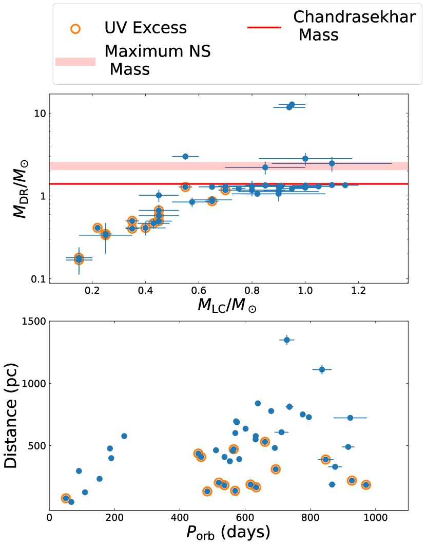
Figure 1: Top: ${M_{\rm{LC}}}$ vs ${M_{\rm{DR}}}$. Each blue dot is a candidate from the ATF22 and SHA23 catalogs. Orange open circles show the candidates for which we found UV excess. The red line shows the Chandrasekhar mass limit and the red-shaded region is the expected limiting mass for NSs. Bottom: ${P_{\rm{orb}}}$ vs Distance for the same sources. All of them are in detached wide orbits and relatively close from us. Blue dots and orange circles have the same meaning.

In this study, we investigate the spectral energy distribution (SED) of selected candidate DR–LC binaries from the ATF22 and SHA23 catalogues in wavelengths spanning ultraviolet (UV), optical, and infrared (IR), and aim to constrain the stellar properties of the components. All sources in these catalogues are expected to have a MS star as the LC in wide orbits (${P_{\rm{orb}}}>45\,{\rm{day}}$) to a DR. Such wide orbits make it very unlikely for active ongoing mass transfer at present. Interestingly, all of these sources are within $1.5\,{\rm{kpc}}$ making them easy targets for follow-up studies (Figure 1).

A SED is the end result of a compilation of images across the electromagnetic spectrum. When such multi-wavelength coverage is available, SEDs have been commonly used to reveal the individual components of an unresolved source. SED analysis can be particularly powerful if the components have significantly different ${T_{\rm{eff}}}$ (Ren et al., 2020; Rebassa-Mansergas et al., 2021). If the DRs in the candidate binaries are non-accreting NSs or BHs, then the SED is not expected to show any statistically significant excess in the UV flux relative to what can be explained by the SED of the LC. On the other hand, if instead, the DR is a WD, then depending on the age, the WD can contribute significantly to the UV flux. As a result, the source’s SED would exhibit significant UV excess compared to what is expected of the SED of the LC alone. In either case, SED analysis can constrain the LC’s stellar properties such as mass (${M_{\rm{LC}}}$), effective temperature (${T_{\rm{eff},LC}}$), metallicity, and bolometric luminosity (${L_{\rm{bol},LC}}$). In combination with Gaia’s astrometric constraints, e.g., for $f_{M}$ or the astrometric mass ratio function (AMRF) the estimated ${M_{\rm{LC}}}$ can also put constraints on the mass of the DR (${M_{\rm{DR}}}$). In case, a significant UV excess is found which can be fitted by a WD, then in addition, we can also estimate the ${T_{\rm{eff}}}$ and ${L_{\rm{bol}}}$ of the candidate WD.

We discuss how we select candidates and observational data for our analysis, model the SEDs and estimate masses for each source in section 2. We show our key results in section 3. Finally, we discuss the implications of our results and future avenues to improve the characterisation of similar sources in section 4.

Table 1: Candidates from ATF22 and SHA23 catalogs with GALEX UV counterparts.

Object	Gaia  DR3 ID	RA	DEC	Parameters from Gaia  DR3				$A_{v}$	Our estimates
		(deg)	(deg)						LC				DR
				${P_{\rm{orb}}}$	e	AMRF	[Fe/H]		${T_{\rm{eff}}}$	$L_{\rm{bol}}$	[Fe/H]	${M_{\rm{LC}}}$	${M_{\rm{DR}}}$
				($10^{2}\,{\rm{day}}$)			(dex)		($10^{3}\,\rm{K}$)	$L_{\odot}$	(dex)	($M_{\odot}$)	($M_{\odot}$)
sources with significant observed UV excess
0812$+$7046	1098489704734299648	123.04	70.78	9.71 $\pm$ 0.12	0.10 $\pm$ 0.01	0.68 $\pm$ 0.03	-0.43	0.08	3.50 $\pm$ 0.12	0.02 $\pm$ 0.00	-0.5 $\pm$ 0.25	0.15 $\pm$ 0.05	0.17 $\pm$ 0.06
1220$+$5841	1581117310088807552	185.05	58.69	9.27 $\pm$ 0.06	0.52 $\pm$ 0.01	1.05 $\pm$ 0.03	$\cdots$	0.04	4.25$\pm$ 0.12	0.08$\pm$ 0.00	0.2$\pm$ 0.12	0.55$\pm$ 0.03	1.28$\pm$ 0.06
2106$-$5218	6476764747694402560	316.53	-52.31	8.47 $\pm$ 0.24	0.08 $\pm$ 0.04	0.76 $\pm$ 0.04	-1.82	0.11	3.75 $\pm$ 0.12	0.05 $\pm$ 0.00	-2.0 $\pm$ 0.25	0.25 $\pm$ 0.10	0.34 $\pm$ 0.13
0824$+$2300	678085695778294784	126.06	23.00	6.94 $\pm$ 0.06	0.13 $\pm$ 0.07	0.67 $\pm$ 0.04	-0.58	0.10	3.75 $\pm$ 0.12	0.04 $\pm$ 0.00	-0.5 $\pm$ 0.25	0.43 $\pm$ 0.06	0.47 $\pm$ 0.07
0709$+$7052	1109902566711892352	107.26	70.87	6.61 $\pm$ 0.06	0.36 $\pm$ 0.03	0.81 $\pm$ 0.04	0.02	0.16	4.25 $\pm$ 0.12	0.09 $\pm$ 0.01	0.0 $\pm$ 0.18	0.45 $\pm$ 0.08	0.67 $\pm$ 0.11
2338$-$7152	6380360186645909760	354.60	-71.88	6.34 $\pm$ 0.02	0.01 $\pm$ 0.02	0.69 $\pm$ 0.03	$\cdots$	0.08	3.50$\pm$ 0.12	0.02$\pm$ 0.00	-0.5$\pm$ 0.25	0.35$\pm$ 0.03	0.40$\pm$ 0.03
0124$+$0758	2566461354152574976	21.05	7.98	6.17 $\pm$ 0.04	0.05 $\pm$ 0.04	0.71 $\pm$ 0.04	-0.30	0.15	3.50 $\pm$ 0.12	0.02 $\pm$ 0.00	-0.5 $\pm$ 0.25	0.15 $\pm$ 0.05	0.18 $\pm$ 0.06
0358$-$8154	4616146191642331008	59.50	-81.90	5.69 $\pm$ 0.02	0.09 $\pm$ 0.02	0.78 $\pm$ 0.05	$\cdots$	0.19	3.75$\pm$ 0.12	0.01$\pm$ 0.00	-1.0$\pm$ 0.25	0.25$\pm$ 0.03	0.35$\pm$ 0.03
0327$-$4342	4847718871053268480	51.83	-43.71	5.65 $\pm$ 0.05	0.33 $\pm$ 0.04	0.76 $\pm$ 0.03	$\cdots$	0.04	4.50$\pm$ 0.12	0.17$\pm$ 0.01	0.2$\pm$ 0.12	0.65$\pm$ 0.03	0.87$\pm$ 0.03
1143$-$2807	3484138291549376128	175.97	-28.12	5.37 $\pm$ 0.03	0.09 $\pm$ 0.04	0.93 $\pm$ 0.07	-0.74	0.30	3.50 $\pm$ 0.12	0.01 $\pm$ 0.00	-0.5 $\pm$ 0.25	0.22 $\pm$ 0.00	0.41 $\pm$ 0.00
2001$-$4438	6685604337007194368	300.31	-44.63	5.19 $\pm$ 0.02	0.06 $\pm$ 0.03	0.64 $\pm$ 0.02	$\cdots$	0.15	3.75$\pm$ 0.12	0.04$\pm$ 0.00	-0.5$\pm$ 0.25	0.40$\pm$ 0.08	0.41$\pm$ 0.08
0338$+$3913	224549450109569536	54.63	39.23	4.84 $\pm$ 0.01	0.03 $\pm$ 0.01	0.67 $\pm$ 0.03	0.07	0.47	3.75 $\pm$ 0.12	0.03 $\pm$ 0.00	0.2 $\pm$ 0.12	0.45 $\pm$ 0.05	0.50 $\pm$ 0.06
1330$+$2827	1449731030688880512	202.65	28.46	4.65 $\pm$ 0.02	0.29 $\pm$ 0.03	0.74 $\pm$ 0.02	-0.15	0.05	4.50 $\pm$ 0.12	0.25 $\pm$ 0.01	-0.5 $\pm$ 0.25	0.45 $\pm$ 0.07	0.58 $\pm$ 0.10
0640$-$2621	2919995917769953408	100.03	-26.36	4.57 $\pm$ 0.02	0.75 $\pm$ 0.05	0.87 $\pm$ 0.04	0.10	0.40	5.25 $\pm$ 0.12	0.21 $\pm$ 0.01	0.2 $\pm$ 0.12	0.70 $\pm$ 0.03	1.18 $\pm$ 0.04
1606$+$6120	1626845895609073536	241.56	61.35	0.51 $\pm$ 0.00	0.02 $\pm$ 0.02	0.79 $\pm$ 0.04	$\cdots$	0.04	3.50$\pm$ 0.12	0.02$\pm$ 0.00	-1.5$\pm$ 0.25	0.35$\pm$ 0.02	0.50$\pm$ 0.04
other sources
1007$+$4453	809741149368202752	151.79	44.90	9.22 $\pm$ 0.51	0.35 $\pm$ 0.03	0.96 $\pm$ 0.04	-0.09	0.03	5.25 $\pm$ 0.12	0.45 $\pm$ 0.03	0.0 $\pm$ 0.18	0.65 $\pm$ 0.05	1.29 $\pm$ 0.10
2244$-$2236	2397135910639986304	341.20	-22.60	9.16 $\pm$ 0.19	0.56 $\pm$ 0.03	0.84 $\pm$ 0.03	-0.17	0.07	6.25 $\pm$ 0.12	0.85 $\pm$ 0.03	0.0 $\pm$ 0.18	0.85 $\pm$ 0.05	1.34 $\pm$ 0.08
0336$+$1419	41408333753757056	54.13	14.32	8.76 $\pm$ 0.21	0.53 $\pm$ 0.03	0.84 $\pm$ 0.03	0.00	1.54	6.75 $\pm$ 0.12	0.31 $\pm$ 0.01	0.0 $\pm$ 0.18	$\cdots$ $\pm$  $\cdots$	$\cdots$ $\pm$  $\cdots$
1012$-$3537	5446310318525312768	153.10	-35.62	8.67 $\pm$ 0.11	0.25 $\pm$ 0.00	0.70 $\pm$ 0.02	$\cdots$	0.38	7.00$\pm$ 0.12	2.41$\pm$ 0.05	0.2$\pm$ 0.12	1.15$\pm$ 0.05	1.35$\pm$ 0.06
1048$+$6547	1058875159778407808	162.25	65.80	8.36 $\pm$ 0.29	0.42 $\pm$ 0.04	0.85 $\pm$ 0.04	-0.19	0.04	6.00 $\pm$ 0.12	1.45 $\pm$ 0.10	0.0 $\pm$ 0.18	0.80 $\pm$ 0.10	1.30 $\pm$ 0.16
1205$+$6914	1683575679079854848	181.35	69.24	7.96 $\pm$ 0.08	0.62 $\pm$ 0.03	0.72 $\pm$ 0.02	0.42	0.05	5.75 $\pm$ 0.12	0.76 $\pm$ 0.02	0.5 $\pm$ 0.15	1.10 $\pm$ 0.05	1.36 $\pm$ 0.06
1622$+$1647	4466767229088016256	245.63	16.80	7.77 $\pm$ 0.05	0.15 $\pm$ 0.03	0.70 $\pm$ 0.03	-0.26	0.14	5.75 $\pm$ 0.12	1.44 $\pm$ 0.08	-0.5 $\pm$ 0.25	0.90 $\pm$ 0.18	1.06 $\pm$ 0.21
1432$-$1021	6328149636482597888	218.09	-10.37	7.36 $\pm$ 0.12	0.14 $\pm$ 0.04	1.03 $\pm$ 0.04	-1.50	0.28	6.00 $\pm$ 0.12	3.02 $\pm$ 0.22	-1.5 $\pm$ 0.25	1.10 $\pm$ 0.23	2.47 $\pm$ 0.51
1812$+$2409	4578398926673187328	273.06	24.15	7.28 $\pm$ 0.23	0.56 $\pm$ 0.05	0.80 $\pm$ 0.04	-0.14	0.39	6.00 $\pm$ 0.12	1.80 $\pm$ 0.11	0.0 $\pm$ 0.18	0.80 $\pm$ 0.13	1.18 $\pm$ 0.18
0036$-$0932	2426116249713980416	9.05	-9.54	7.12 $\pm$ 0.21	0.40 $\pm$ 0.03	0.80 $\pm$ 0.03	-0.56	0.11	5.75 $\pm$ 0.12	1.85 $\pm$ 0.13	-0.5 $\pm$ 0.25	0.91 $\pm$ 0.09	1.32 $\pm$ 0.14
1949$+$0129	4240540718818313984	297.43	1.49	6.91 $\pm$ 0.02	0.62 $\pm$ 0.02	0.86 $\pm$ 0.02	-0.07	0.85	5.75 $\pm$ 0.12	0.48 $\pm$ 0.02	0.0 $\pm$ 0.18	0.75 $\pm$ 0.03	1.23 $\pm$ 0.04
2228$-$3943	6593763230249162112	337.21	-39.72	6.80 $\pm$ 0.03	0.61 $\pm$ 0.07	0.86 $\pm$ 0.04	-0.06	0.05	6.00 $\pm$ 0.12	1.76 $\pm$ 0.09	0.0 $\pm$ 0.18	0.80 $\pm$ 0.13	1.32 $\pm$ 0.21
0217$-$7541	4637171465304969216	34.46	-75.70	6.39 $\pm$ 0.04	0.37 $\pm$ 0.03	0.80 $\pm$ 0.02	0.05	0.15	5.75 $\pm$ 0.12	1.45 $\pm$ 0.04	0.0 $\pm$ 0.18	0.90 $\pm$ 0.05	1.30 $\pm$ 0.07
1150$-$2203	3494029910469026432	177.72	-22.06	6.33 $\pm$ 0.02	0.55 $\pm$ 0.02	0.74 $\pm$ 0.02	0.21	0.13	6.00 $\pm$ 0.12	2.30 $\pm$ 0.06	0.2 $\pm$ 0.12	1.00 $\pm$ 0.05	1.29 $\pm$ 0.06
1449$+$6919	1694708646628402048	222.33	69.32	6.32 $\pm$ 0.03	0.26 $\pm$ 0.02	0.73 $\pm$ 0.02	-0.71	0.09	6.00 $\pm$ 0.12	1.28 $\pm$ 0.04	-0.5 $\pm$ 0.25	1.00 $\pm$ 0.05	1.26 $\pm$ 0.06
1310$+$6016	1579254496872812032	197.71	60.28	6.01 $\pm$ 0.03	0.31 $\pm$ 0.03	0.74 $\pm$ 0.02	-0.69	0.04	5.25 $\pm$ 0.12	0.53 $\pm$ 0.01	-0.5 $\pm$ 0.25	0.82 $\pm$ 0.06	1.06 $\pm$ 0.08
0109$-$1034	2469926638416055168	17.37	-10.58	5.82 $\pm$ 0.04	0.74 $\pm$ 0.06	1.03 $\pm$ 0.07	-0.17	0.08	4.75 $\pm$ 0.12	0.09 $\pm$ 0.00	-0.5 $\pm$ 0.25	0.45 $\pm$ 0.08	1.02 $\pm$ 0.17
2100$-$2535∗	6802561484797464832	315.11	-25.59	5.75 $\pm$ 0.06	0.83 $\pm$ 0.07	1.11 $\pm$ 0.16	-0.22	0.25	6.25 $\pm$ 0.12	2.98 $\pm$ 0.13	0.0 $\pm$ 0.18	0.85 $\pm$ 0.15	2.21 $\pm$ 0.39
1733$+$5808	1434445448240677376	263.40	58.15	5.72 $\pm$ 0.02	0.30 $\pm$ 0.02	0.73 $\pm$ 0.02	-0.21	0.13	5.75 $\pm$ 0.12	1.37 $\pm$ 0.03	-0.5 $\pm$ 0.25	0.90 $\pm$ 0.15	1.13 $\pm$ 0.19
1046$+$1002	3869650535947137920	161.52	10.05	5.70 $\pm$ 0.05	0.18 $\pm$ 0.04	0.84 $\pm$ 0.04	-0.09	0.08	6.25 $\pm$ 0.12	1.87 $\pm$ 0.08	0.0 $\pm$ 0.18	0.85 $\pm$ 0.08	1.35 $\pm$ 0.12
0003$-$5604	4922744974687373440	0.86	-56.08	5.62 $\pm$ 0.02	0.81 $\pm$ 0.03	0.92 $\pm$ 0.07	$\cdots$	0.04	5.00$\pm$ 0.12	0.29$\pm$ 0.01	0.0$\pm$ 0.18	0.70$\pm$ 0.05	1.30$\pm$ 0.09
0119$-$2526	5039979680444075392	19.79	-25.44	5.53 $\pm$ 0.01	0.18 $\pm$ 0.01	0.73 $\pm$ 0.02	0.03	0.05	5.75 $\pm$ 0.12	0.87 $\pm$ 0.02	0.2 $\pm$ 0.12	1.05 $\pm$ 0.05	1.30 $\pm$ 0.06
0152$-$2049	5136025521527939072	28.21	-20.82	5.37 $\pm$ 0.01	0.65 $\pm$ 0.01	0.74 $\pm$ 0.02	-1.39	0.05	6.50 $\pm$ 0.12	2.07 $\pm$ 0.04	-1.0 $\pm$ 0.25	0.90 $\pm$ 0.06	1.16 $\pm$ 0.07
0334$+$0009	3263804373319076480	53.73	0.15	5.11 $\pm$ 0.05	0.28 $\pm$ 0.02	1.15 $\pm$ 0.11	-1.26	0.35	5.75 $\pm$ 0.12	1.89 $\pm$ 0.08	-1.0 $\pm$ 0.25	1.00 $\pm$ 0.18	2.82 $\pm$ 0.49
2057$-$4742	6481502062263141504	314.49	-47.70	2.30 $\pm$ 0.01	0.30 $\pm$ 0.04	0.74 $\pm$ 0.02	$\cdots$	0.14	6.25$\pm$ 0.12	0.98$\pm$ 0.03	0.2$\pm$ 0.12	0.95$\pm$ 0.05	1.23$\pm$ 0.06
0553$-$1349	2995961897685517312	88.47	-13.83	1.90 $\pm$ 0.00	0.37 $\pm$ 0.07	0.76 $\pm$ 0.03	-0.46	1.07	7.25 $\pm$ 0.12	1.78 $\pm$ 0.03	-0.5 $\pm$ 0.25	1.00 $\pm$ 0.05	1.34 $\pm$ 0.07
1728$-$0034	4373465352415301632	262.17	-0.58	1.86 $\pm$ 0.00	0.49 $\pm$ 0.07	2.26 $\pm$ 0.17	-1.07	1.23	6.25 $\pm$ 0.12	1.43 $\pm$ 0.03	-1.0 $\pm$ 0.25	0.95 $\pm$ 0.05	12.74 $\pm$ 0.67
1452$-$1922	6281177228434199296	223.21	-19.37	1.54 $\pm$ 0.00	0.18 $\pm$ 0.04	2.21 $\pm$ 0.11	-0.54	0.29	5.75 $\pm$ 0.12	1.65 $\pm$ 0.03	-0.5 $\pm$ 0.25	0.94 $\pm$ 0.06	11.75 $\pm$ 0.75
1301$-$1852	3509370326763016704	195.32	-18.87	1.09 $\pm$ 0.00	0.24 $\pm$ 0.02	1.57 $\pm$ 0.04	-0.19	0.32	4.75 $\pm$ 0.12	0.18 $\pm$ 0.00	0.0 $\pm$ 0.18	0.55 $\pm$ 0.05	3.00 $\pm$ 0.27
0632$-$6614	5283631903842076032	98.17	-66.24	0.91 $\pm$ 0.00	0.31 $\pm$ 0.04	0.77 $\pm$ 0.03	-0.22	0.17	5.00 $\pm$ 0.12	0.39 $\pm$ 0.00	-0.5 $\pm$ 0.25	0.65 $\pm$ 0.08	0.90 $\pm$ 0.10
0156$+$1228	2574867704662509568	29.15	12.47	0.68 $\pm$ 0.00	0.56 $\pm$ 0.03	0.81 $\pm$ 0.03	$\cdots$	0.25	4.25$\pm$ 0.12	0.20$\pm$ 0.00	-1.5$\pm$ 0.25	0.57$\pm$ 0.08	0.85$\pm$ 0.11
						$f_{M}$(${M_{\odot}}$)
1007$+$3408	747174436620510976	151.84	34.14	9.99$\pm$0.26	0.71$\pm$0.02	$0.56^{+0.05}_{-0.04}$	-0.02	0.04	5.5$\pm$0.1	$0.30\pm 0.02$	0.0$\pm$0.2	$0.6\pm 0.1$	$1.2^{+0.2}_{-0.1}$
1433$-$0114	3649963989549165440	218.38	-1.25	8.93$\pm$0.60	0.36$\pm$0.14	0.8 ${}^{+0.5}_{-0.2}$	0.01	0.13	24$\pm$1	$8.1\pm 0.1$	0.0$\pm$0.2	$\cdots$	$\cdots$
2033$+$0758	1749013354127453696	308.31	7.98	9.32$\pm$0.78	0.51$\pm$ 0.08	0.8 ${}^{+0.6}_{-0.4}$	-0.27	0.30	6.0$\pm$0.1	$4.0\pm 0.1$	0.0$\pm$0.2	$1.0\pm 0.5$	$1.9^{+1.2}_{-0.9}$

Note. — Properties of 49 sources from the ATF22 and SHA23 catalogs with GALEX counterparts. The sources are sorted by their ${P_{\rm{orb}}}$. Parameters we estimate and those found in Gaia’s DR3 and its non-single star catalog are noted separately. Errors in AMRF (for SHA23), $f_{M}$ ( for ATF22) and ${P_{\rm{orb}}}$ denote $95\%$ confidence interval. Our estimated for ${T_{\rm{eff}}}$ and [Fe/H] for the LC come from SED modelling with uncertainty denoting half of the grid spacing for the SED models. ${L_{\rm{bol}}}$ measurement and their corresponding errors come from the observed flux and Gaia-estimated distances. We did not model 1433$-$0114, a hot sub-dwarf (Boudreaux et al., 2017; Geier et al., 2017). * denotes low (6.82) significance for the astrometric solution.

2 Data Selection and Mass estimation

2.1 Data Selection and SED fitting

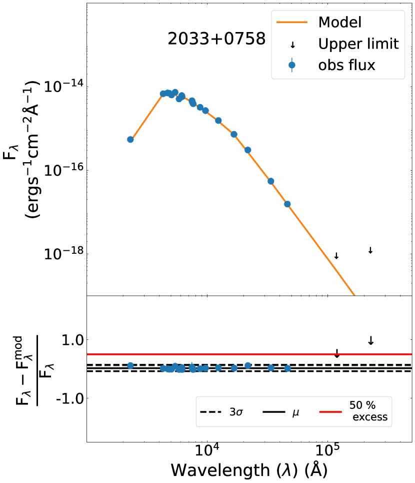
Figure 2: Flux density (per unit wavelength, $F_{\lambda}$) vs wavelength ($\lambda$) for source 2033$+$0758 (Table 1), as an example of a source exhibiting no significant (c.f., subsection 2.1) UV excess. Blue dots and orange line show the observed and best-fit synthetic $F_{\lambda}$ assuming a single-component MS star SED. Black arrows for IR flux denote upper limits. Bottom: Fractional residuals (blue dots) vs $\lambda$. We show the mean of the residual flux ratios (blue solid), $3\sigma$ limits centering the mean (black dashed), and $50\%$ excess from the mean (red solid line). Similar figures with single-component SEDs for the other sources are available online.

We cross match 187 DR–LC candidate sources listed in the ATF22 and SHA23 catalogs with the GALEX archival data (Bianchi et al., 2017) using 3^′′ radius and find unique UV counterparts for 49 sources. The properties and call names for these sources are listed in Table 1. We cross-match these 49 sources with APASS DR9 (Henden et al., 2015) and PanSTARRS-DR2 (Magnier et al., 2020) in the optical, and 2MASS (Skrutskie et al., 2006), ALLWISE (Wright et al., 2010) in the IR to construct the SED from UV to Near-IR (NIR). Often only the limiting IR flux is available, in these cases, we use the IR flux as an upper limit but do not use it for the SED fitting. We use the Kurucz model spectra (Castelli et al., 1997) in a large range of $\log(g/{\rm{cm\ s^{-2}}})=4$–$5$ and effective temperature ${T_{\rm{eff}}}/{\rm K}=3,500$–$50,000$ to fit the observed SEDs by synthetic MS star SEDs spanning NUV to NIR using the widely used and publicly available VOSA utility which estimates the best-fit stellar parameters based on astronomical input and available observed fluxes using $\chi^{2}$ optimization (Bayo et al., 2008a, b). We provide astronomical input to the VOSA utility while fitting the SED of each source. For example, we adopt the interstellar extinction values listed in the GALEX  catalog ($A_{v}$; Schlegel et al., 1998), the Gaia-estimated parallax for each source (Gaia Collaboration et al., 2022a), and use bounds around the Gaia-estimated photometric metallicity (Gaia Collaboration et al., 2022b). Figure 2 shows source 2033$+$0758 as an example where the observed SED can be fitted with a single-component MS star. The best-fit SED provides us with a variety of stellar parameters for the LC including metallicity, ${T_{\rm{eff},LC}}$, ${L_{\rm{bol},LC}}$, and ${\log\ g_{\rm{LC}}}$.

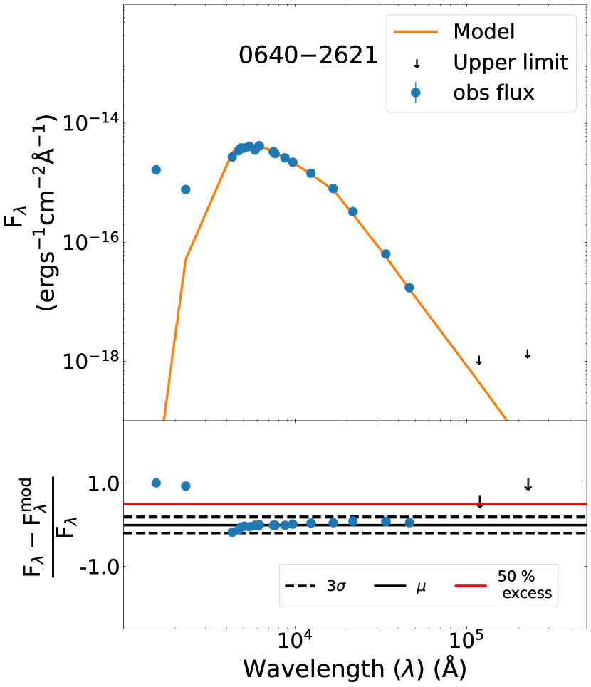
Figure 3: Same as Figure 2, but for source 0640$-$2621 which exhibits significant UV excess relative to the best-fit MS star SED.

For each source, we analyze the residuals in the observed SED with respect to the best-fit model SED of a MS star obtained from VOSA. If the UV flux is higher than three times the standard deviation found in the residuals across optical and IR, and shows a fractional excess of above $50\%$ in the UV, we consider that the source exhibits a significant UV excess. Note that these are stringent requirements; the latter ensures significant excess in UV flux and the former ensures that the excess is significantly higher compared to residuals in other bands. Figure 3 shows source 0640$-$2621 as an example with significant excess in FUV and NUV. If significant UV excess is found, we fit a composite MS–WD model to the observed SED to extract the WD properties including ${T_{\rm{eff,WD}}}$ and ${L_{\rm{bol,WD}}}$, and update the LC properties. To model the contribution of the WD to the combined SED, we adopt the widely used Koester DA-type WD model spectra (Koester, 2010) in the range ${T_{\rm{eff}}}/{\rm K}=5,000$–$80,000$ and $\log(g/{\rm{cm\ s^{-2}}})=6.5$–$9.5$. We use VOSA-recommended Visual goodness of fit (Vgf_b), similar to reduced $\chi^{2}$, but adopted for unknown or wrongly reported small flux errors, to justify composite SED fits Bayo et al. (2008b). When excess is found, the composite fit significantly improves $\rm{Vgf_{b}}$ (Table 2).

2.2 Mass Estimates

Single component (MS star only if there is no UV excess) or multi-component (MS–WD if there is significant UV excess) SED modelling provides us with excellent constraints on ${L_{\rm{bol}}}$, ${T_{\rm{eff}}}$, and the radius of the source (and components). However, we notice that the constraint on mass from the SED modelling is rather weak. This is because SEDs are not sufficiently sensitive to $\log\ g$ and this results in large errors in the estimated mass (Bayo et al., 2008b). Hence, we constrain ${M_{\rm{LC}}}$ using stellar evolution models created via MIST (Dotter, 2016; Choi et al., 2016; Paxton et al., 2011, 2013, 2015, 2018) and the constraints on the metallicity, ${L_{\rm{bol},LC}}$, and ${T_{\rm{eff},LC}}$ found from SED modeling. In particular, using MIST, we evolve stars within a reasonable range ($0.10$–$1.45\,{M_{\odot}}$ with a grid resolution of $0.015\,{M_{\odot}}$) in zero-age MS mass from pre-MS to the MS turn-off adopting metallicity from the best-fit parameters of the SED. We create small 2D boxes around the SED-estimated ${L_{\rm{bol},LC}}$ and ${T_{\rm{eff},LC}}$ values for each source. The width and height of these small boxes are adopted to be $\delta{L_{\rm{bol}}}/{L_{\rm{bol}}}=\delta{T_{\rm{eff}}}/{T_{\rm{eff}}}=\pm 5\%$. These adopted fractional errors are typical of SED modelling errors obtained from VOSA. We collect all stellar tracks passing through this box and assign ${M_{\rm{LC}}}$ to the median value of the stellar masses for these tracks. The error in ${M_{\rm{LC}}}$ is assigned to be the difference between the $25$ and $75$th percentiles for these masses.

Astrometric solutions are thought to be acceptable if goodness of fit $<25$ and significance $>12$ (Halbwachs et al., 2022). We find that the maximum goodness of fit for our sources is 11.3. On the other hand, except for source 2100$-$2535 with a significance 6.82 all other sources have a significance $>12$, median, 5th, and 95th percentiles are 47.75, 14.03, 119.43. We use our estimated ${M_{\rm{LC}}}$ and

$$\mathrm{AMRF}=\frac{{M_{\rm{DR}}}/{M_{\rm{LC}}}}{(1+{M_{\rm{DR}}}/{M_{\rm{LC}}})^{2/3}}$$ (1)

or

$$f_{M}=\frac{{M_{\rm{DR}}}^{3}}{({M_{\rm{DR}}}+{M_{\rm{LC}}})^{2}}$$ (2)

calculated from Gaia’s astrometric solution to estimate ${M_{\rm{DR}}}$ for sources in the SHA23 or ATF22 catalogs, respectively. Hence, the ${M_{\rm{DR}}}$ estimates depend on the accuracy of the astrometric solutions.

3 Results

3.1 Sources showing significant UV excess

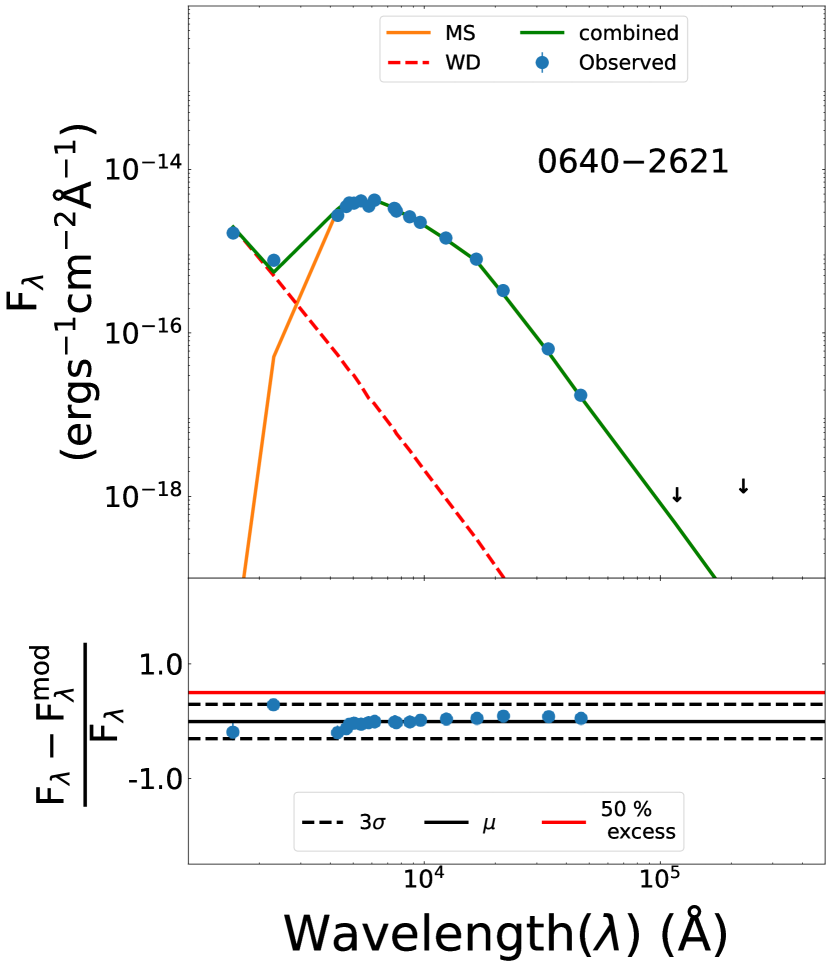
Figure 4: SEDs and residuals for 0640$-$2621 showing significant UV excess. In the SED panels, the orange solid (red dashed) line shows the best-fit synthetic SED for the MS (WD) star. The solid green line shows the combined MS–WD flux. Blue dots denote observed flux (subsection 2.1). Lines and symbols in the residual panels have the same meaning as in Figure 3. The complete figure set (15 images) is available in the online journal.

Table 2: Properties of the candidate WDs.

Object	UV	${T_{\rm{eff}}}$	${L_{\rm{bol}}}$	$\log\ (g/{\rm{cm\ s^{-2}}})$	${M_{\rm{DR}}}$	% Vgfb	SHA23
		$(10^{3}\,\rm{K})$	$(L_{\odot})$		$({M_{\odot}})$	Improvement${}^{\tablenotemark{a}}$	Classification
0812$+$7046	N	12.00 $\pm$ 0.12	0.0014 $\pm$ 0.0001	9.00 $\pm$ 0.12	0.17 $\pm$ 0.06	87	WD
1220$+$5841	N	7.00 $\pm$ 0.12	0.0029 $\pm$ 0.0004	9.00 $\pm$ 0.12	1.28 $\pm$ 0.06	41	NS
2106$-$5218	N	10.00 $\pm$ 0.12	0.0023 $\pm$ 0.0003	6.00 $\pm$ 0.12	0.34 $\pm$ 0.13	43	WD
0824$+$2300	B	17.50 $\pm$ 0.12	0.0021 $\pm$ 0.0003	9.00 $\pm$ 0.12	0.47 $\pm$ 0.07	71	WD
0709$+$7052	B	16.00 $\pm$ 0.12	0.0036 $\pm$ 0.0017	9.00 $\pm$ 0.12	0.67 $\pm$ 0.11	86	NS
2338$-$7152	N	80.00 $\pm$ 0.50	0.0014 $\pm$ 0.0001	9.00 $\pm$ 0.12	0.40 $\pm$ 0.03	99	WD
0124$+$0758	N	6.75 $\pm$ 0.12	0.0031 $\pm$ 0.0002	8.00 $\pm$ 0.12	0.18 $\pm$ 0.06	-50	WD
0358$-$8154	N	80.00 $\pm$ 0.50	0.0028 $\pm$ 0.0001	9.00 $\pm$ 0.12	0.35 $\pm$ 0.03	89	WD
0327$-$4342	N	13.00 $\pm$ 0.12	0.0024 $\pm$ 0.0008	9.00 $\pm$ 0.12	0.87 $\pm$ 0.03	86	NS
1143$-$2807	N	14.50 $\pm$ 0.12	0.0005 $\pm$ 0.0001	6.00 $\pm$ 0.12	0.41 $\pm$ 0.00	76	WD
2001$-$4438	B	14.50 $\pm$ 0.12	0.0017 $\pm$ 0.0002	9.00 $\pm$ 0.12	0.41 $\pm$ 0.08	74	WD
0338$+$3913	N	17.00 $\pm$ 0.12	0.0032 $\pm$ 0.0002	9.00 $\pm$ 0.12	0.50 $\pm$ 0.06	25	WD
1330$+$2827	N	7.75 $\pm$ 0.12	0.0105 $\pm$ 0.0030	9.00 $\pm$ 0.12	0.58 $\pm$ 0.10	24	NS
0640$-$2621	B	50.00 $\pm$ 0.38	0.0269 $\pm$ 0.0014	6.00 $\pm$ 0.12	1.18 $\pm$ 0.04	88	NS
1606$+$6120	N	10.25 $\pm$ 0.12	0.0011 $\pm$ 0.0001	9.00 $\pm$ 0.12	0.50 $\pm$ 0.04	44	WD

Note. — Properties of the 15 sources with significant UV excess. Errors in ${M_{\rm{DR}}}$ is estimated from ${M_{\rm{LC}}}$ errors. ${T_{\rm{eff}}}$ and $\log\ (g)$ estimates are from SED modeling. Uncertainties denote half of the grid spacing for the SED models. ${L_{\rm{bol}}}$ measurements and their corresponding errors come from the observed flux and Gaia-estimated distances. N, B denote only NUV, both FUV and NUV flux are available. While the composite fit is visibly better (7th figure of Figure 4) than the single component fit for source 0124$+$0758, we do not find a clear improvement in VGf_b.

We find significant UV excess relative to a single-component model SED for 15 of the 49 sources we have analysed. In 4 of these sources (0824$+$2300, 0709$+$7052, 2001$-$4438, and 0640$-$2621) both FUV and NUV data are available and both fluxes show excess. In case of the others, only the NUV flux is available. Using two-component MS–WD synthetic SEDs we are able to fit all of the 15 sources. Figure 4 shows the observed SEDs, best-fit models for the combined two-component models, the MS and WD individual contributions, and the residuals for the 15 sources. Clearly, adding a hot component from a WD to the MS star’s SED significantly improves the fit and the presence of a WD companion can easily explain the observed excess UV flux. We find the stellar properties including [Fe/H], ${L_{\rm{bol}}}$, ${T_{\rm{eff}}}$, and $\log\ (g/{\rm{cm\ s^{-2}}})$ for both components. The stellar properties of the LCs are summarised in Table 1 and those for the WDs are shown in Table 2. In all cases the errors in ${T_{\rm{eff}}}$, [Fe/H], and $\log(g/{\rm{cm\ s^{-2}}})$ denote half of the grid-spacing available in VOSA for the SED modelling, whereas, ${L_{\rm{bol}}}$ error denotes propagated errors from uncertainties in the observed flux and Gaia’s distance measurement.

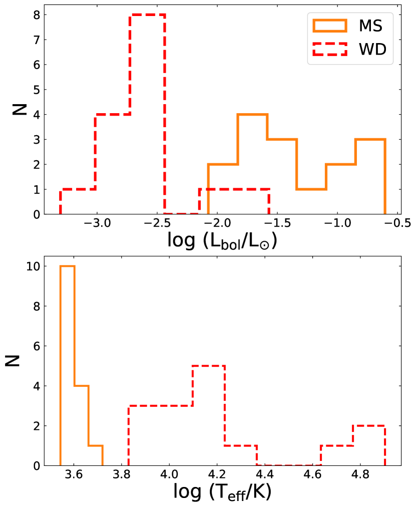
Figure 5: Probability distribution functions for ${L_{\rm{bol}}}$ (top) and ${T_{\rm{eff}}}$ (bottom) for the WDs (red dashed) and MS stars (orange solid) for sources showing significant UV excess.

Figure 5 shows the distributions of ${L_{\rm{bol}}}$ and ${T_{\rm{eff}}}$ for the MS and the WD in these 15 sources. As expected, distributions for ${T_{\rm{eff,WD}}}$ and ${T_{\rm{eff},LC}}$ are well separated with medians ${T_{\rm{eff,WD}}}/\rm{K}=14500\pm 7125$ and ${T_{\rm{eff},LC}}/\rm{K}=5750\pm 1750$. Whereas, the medians for ${L_{\rm{bol,WD}}}/L_{\odot}=0.0024\pm 0.0016$ and ${L_{\rm{bol},LC}}/L_{\odot}=0.51\pm 1.50$. All of these sources are well explained by DA type WDs with pure hydrogen atmosphere.

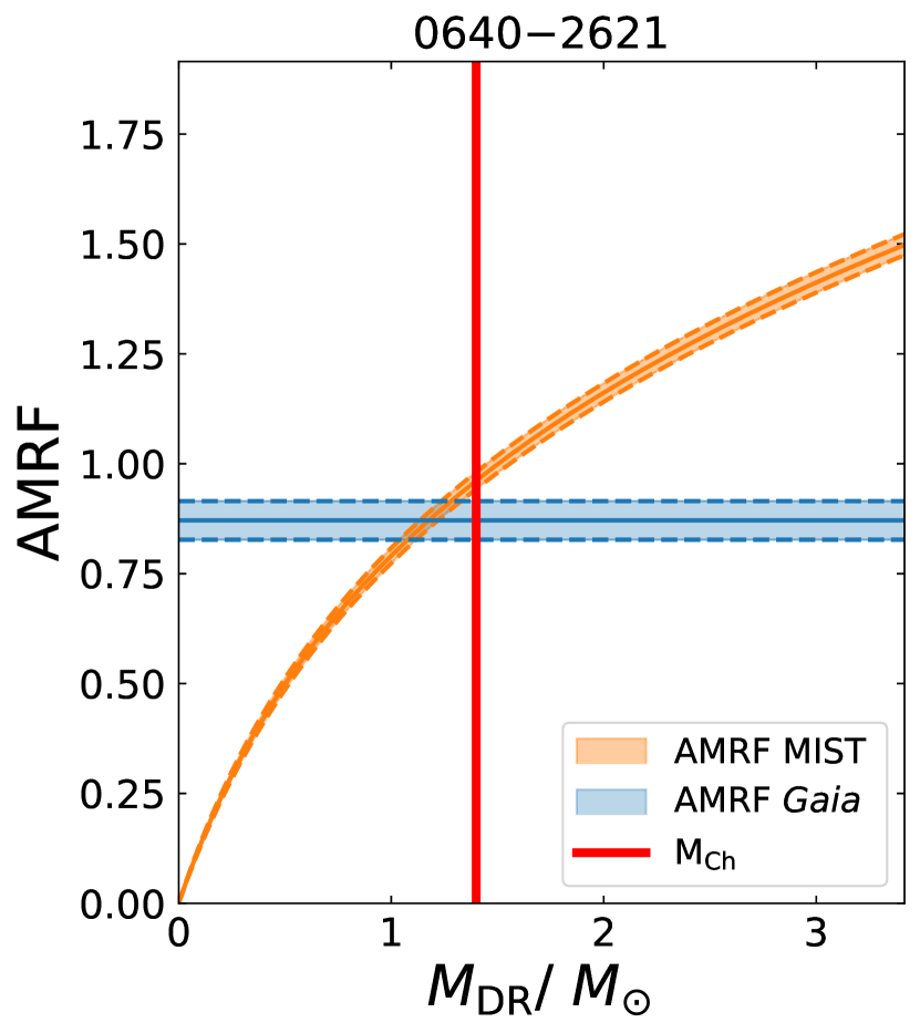
Figure 6: AMRF vs ${M_{\rm{DR}}}$ for 0640$-$2621. The orange-shaded region shows the allowed parameter space based on our estimated ${M_{\rm{LC}}}$ (subsection 3.2). The blue-shaded region shows the estimated AMRF from SHA23. The overlap between the blue and the orange regions is the solution for ${M_{\rm{DR}}}$ that satisfies all available constraints. The red vertical line denotes ${M_{\rm{Ch}}}$. Our results suggest that source 0640$-$2621 hosts a WD. (Similar figures for the other sources are available online.)

Incidentally, all of these 15 sources belong to the SHA23 catalog which provides constraints on the AMRF (Equation 1) from Gaia’s astrometric solutions for these candidate binaries. Adopting the constraints of ${L_{\rm{bol},LC}}$, ${T_{\rm{eff},LC}}$, and [Fe/H] from SED modeling, and using MIST stellar evolution models we constrain ${M_{\rm{LC}}}$ (subsection 2.2). Using ${M_{\rm{LC}}}$ and the constraints on the AMRF we estimate ${M_{\rm{DR}}}$ for these sources (subsection 2.2). Figure 6 shows AMRF vs ${M_{\rm{DR}}}$ using source 0640-2621 as an example. The orange shaded region shows the allowed AMRF values as a function of ${M_{\rm{DR}}}$ adopting our ${M_{\rm{LC}}}$ constraints. The blue shaded region shows the AMRF measured by SHA23 from Gaia DR3. The overlap between the two shaded regions satisfy all available constraints. Clearly, the estimated ${M_{\rm{DR}}}$ for source 0640$-$2621 is below ${M_{\rm{Ch}}}$ denoted by the vertical red line. Indeed, we find that the estimated ${M_{\rm{DR}}}$ for all of these 15 sources are significantly below ${M_{\rm{Ch}}}$. While ${M_{\rm{DR}}}/{M_{\odot}}<1$ for most sources, source 1220$+$5841 exhibits the highest ${M_{\rm{DR}}}/M_{\odot}=1.28\pm 0.06$ with source 0640$-$2621 a close second, ${M_{\rm{DR}}}/{M_{\odot}}=1.18\pm 0.04$ (Table 2). This bolsters our belief that the easiest way to explain the UV excess for these sources is that the DRs in them are indeed WDs.

Interestingly, sources 0812$+$7046, 2106$-$5218, 0124$+$0758, and 0358$-$8154 with ${M_{\rm{DR}}}/{M_{\odot}}<0.4$ are likely so-called extremely low-mass WDs (ELMWD). ELMWDs cannot be created via a single star’s evolution simply because the universe is not old enough for the progenitors to evolve off the MS (Iben, 1990; Iben et al., 1997). ELMWDs are usually observed in compact binaries, the orbital period set by the requirement of mass transfer via Roche-lobe overflow, typically with a WD or a NS companion (Brown et al., 2020). If indeed, these sources host ELMWDs, these would be very interesting sources to study in detail since the LCs are MS stars and the orbital periods are ${P_{\rm{orb}}}/{\rm{day}}>5.6\times 10^{2}$, significantly larger compared to the boundary predicted by the requirement of mass transfer via RLOF (Rappaport et al., 1995; Tauris & Savonije, 1999; Lin et al., 2011; Istrate et al., 2014, 2016). These four ELMWD candidates from our analysis show eccentricity values around 0.1 and a period of 500 - 1000 days. These eccentricities and orbital periods may indicate creation via dynamical processes Khurana et al. (2023).

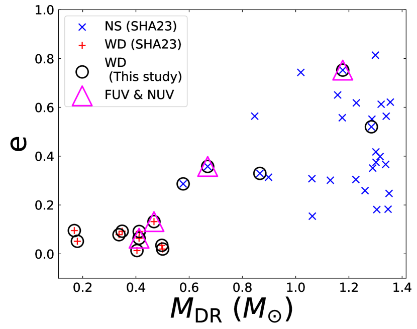
Figure 7: Eccentricity vs ${M_{\rm{DR}}}$ for the 49 sources with identified UV counterparts. Circles denote the 15 sources with significant UV excess. Red + (blue x) denotes sources identified as WDs (NSs) in the SHA23 catalog. In all cases, we use ${M_{\rm{DR}}}$ estimated by this study (subsection 3.3) and the eccentricities given by SHA23. All the magenta triangles show where we have both FUV and NUV data.

Interestingly, SHA23, found that the candidate sources hosting DRs with estimated ${M_{\rm{DR}}}/M_{\odot}<2.1$ likely constitute a mixture of gaussian distributions with peaks that are reasonably well separated in ${M_{\rm{DR}}}$. Based on the gaussian mixture model SHA23 classified these sources into NSs and WDs. Of course, this is a probabilistic classification and can have large uncertainties. Based on Gaussian mixtures, SHA23 classified 0709+7052 and 0640$-$2621 as NSs. Both 0709$+$7052 and 0640$-$2621 show significant excess both in the NUV and FUV. We find ${M_{\rm{DR}}}/{M_{\odot}}=0.7$ ($1.2$) for 0709$+$7052 (0640$-$2621). While mass alone cannot be a clear classifier between WDs and NSs, together with the UV excess both in the FUV and NUV for these sources would suggest that these sources were wrongly classified as NSs by SHA23. We also find significant UV excess in NUV and masses below the NS mass range for 1220$+$5841, 0327$-$4342, and 1330$+$2827 though SHA23 classified them as NSs. The other 10 sources showing significant UV excess and fitted well by a WD as the DR, were also identified as WDs by SHA23.

Figure 7 shows eccentricity vs ${M_{\rm{DR}}}$ for the 15 sources showing significant UV excess and compares them with all SHA23 sources shown in (figure 8 Shahaf et al., 2023). Clearly, the misidentified sources are near the parameter space where the NSs and the WDs are well mixed. This is likely the reason why the gaussian mixture model failed to predict the nature of these two sources correctly. This underlines the power of multi-wavelength followup and SED analysis to identify or confirm the nature of DRs in candidate systems identified by Gaia.

3.2 Sources without significant UV excess

We do not find significant (subsection 2.1) UV excess in the other 34 sources. In these cases, we are able to fit a single-component MS star model to the observed SEDs and estimate ${T_{\rm{eff}}}$, [Fe/H], ${L_{\rm{bol}}}$, and $\log(g/{\rm{cm\ s^{-2}}})$ for the LC. We estimate ${M_{\rm{LC}}}$ for all of these sources using the constraints on the stellar properties and MIST models except for sources 1433$-$0114 and 0336$+$1419. Source 1433$-$0114 has been previously identified as a hot sub-dwarf (Geier et al., 2017; Boudreaux et al., 2017). Being a hot sub-dwarf, source 1433$-$0114 lies in between the MS and the WD regions on a Hertzprung-Russel diagram (HRD). Due to its potentially complex formation history and its unusual position in the HRD (Heber, 2016), we do not attempt to estimate ${M_{\rm{LC}}}$ for 1433$-$0114. In case of 0336$+$1419, we could not find enough MIST isochrones satisfying the constraints on [Fe/H], ${L_{\rm{bol},LC}}$, and ${T_{\rm{eff},LC}}$. All stellar properties as well as ${M_{\rm{LC}}}$ (when available) are summarised in Table 1.

3.3 Estimated masses

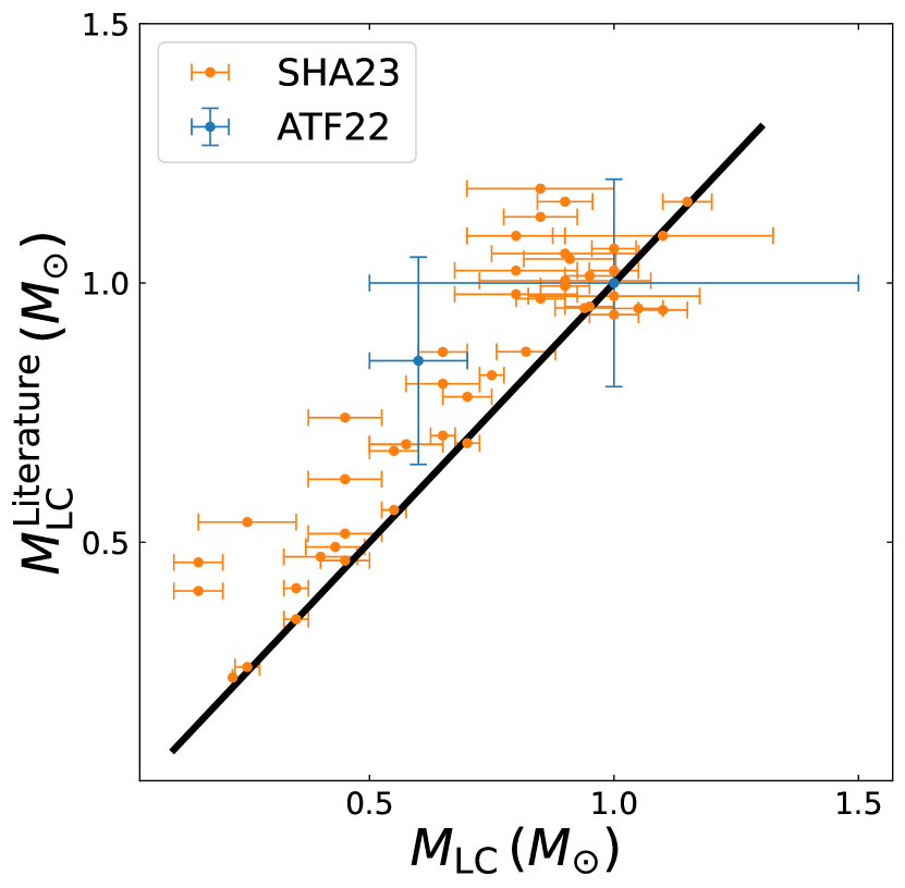
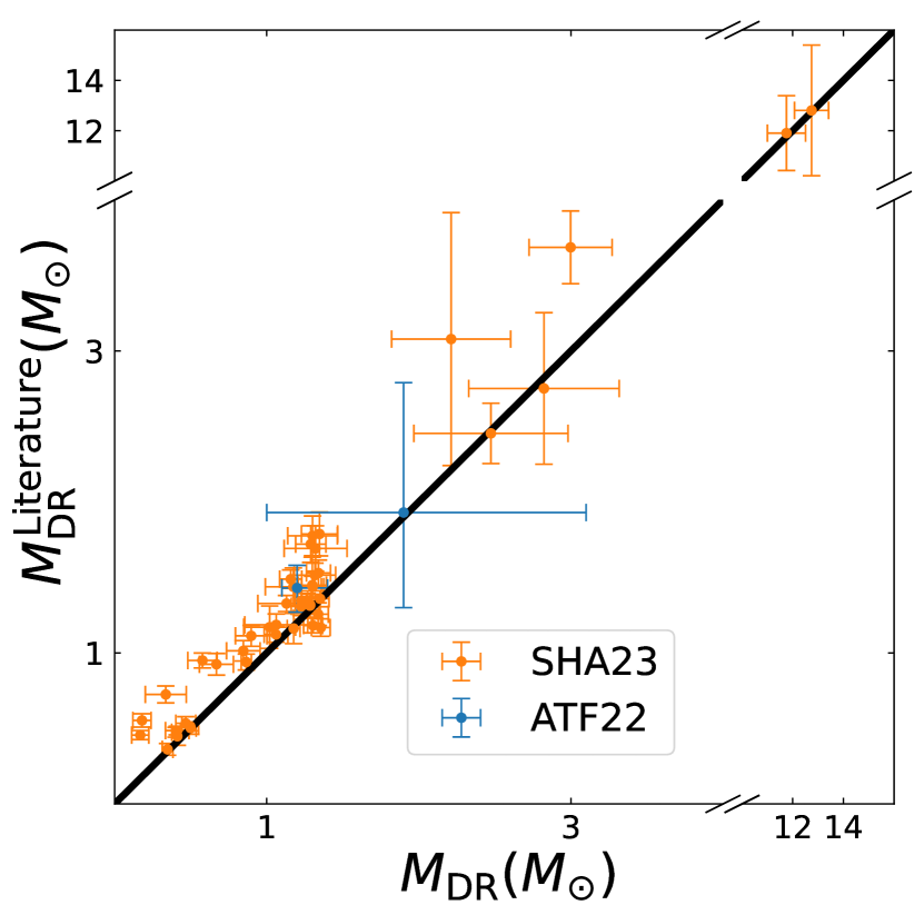
Figure 8: Comparison of mass estimated in this study vs those reported in the SHA23 and ATF22 catalogs for the LCs (left) and DRs (right). Blue (orange) dots show candidates from the ATF22 (SHA23) catalogs. Black solid line shows the $x=y$ line. While more or less consistent, our estimated ${M_{\rm{LC}}}$ and ${M_{\rm{DR}}}$ are typically slightly lower.

Our estimates provide independent measurements of ${M_{\rm{LC}}}$ employing completely different methods compared to the estimated, or often, adopted masses available in the literature. For example, ATF22 estimated ${M_{\rm{LC}}}$ of 1433$-$0114 using the UCO Lick spectra and Apsis and assumed an ad-hoc uncertainty of $0.1\,{M_{\odot}}$. The reported masses of the other ATF22 sources were simply adopted to be between $0.63$ and $1\,{M_{\odot}}$ based on their nominal locations on the Gaia CMD. SHA23 directly used Gaia’s mass estimates, which are derived using PARSEC isochrones and Gaia’s color and magnitude. In contrast, we estimate ${M_{\rm{LC}}}$ uniformly for all our analysed sources using [Fe/H], ${L_{\rm{bol},LC}}$, and ${T_{\rm{eff},LC}}$ constrained by SED modelling and MIST stellar evolution models. Instead of depending only on Gaia colors and magnitude, SED modeling takes into account flux from UV to NIR to constrain the stellar properties which is then used to constrain the mass. In spite of the different methods, our ${M_{\rm{LC}}}$ measurements are more or less in agreement with those estimated or adopted previously in the ATF22 and SHA23 catalogs (left panel Figure 8). Nevertheless, we find that our estimated ${M_{\rm{LC}}}$ is usually slightly lower than the previously adopted or estimated values. Note that these small differences in the estimated ${M_{\rm{LC}}}$ actually push the corresponding ${M_{\rm{DR}}}$ a little lower than was reported in the SHA23 and ATF22 catalogs (right panel Figure 8; Equation 1, 2).

For sources 1728$-$0034 and 1452$-$1922, our estimated ${M_{\rm{DR}}}/{M_{\odot}}\gtrsim 10$ and they show no UV excess. These are good candidates for wide-orbit BH–LC binaries predicted to be present in large numbers in the Milky Way (e.g., Breivik et al., 2017; Chawla et al., 2022). Interestingly, source 1728$-$0034, popularly called the Gaia BH1, has already been identified through radial velocity and astrometric measurements to likely host a BH with ${M_{\rm{DR}}}/{M_{\odot}}=9.8\pm 0.2$ (El-Badry et al., 2023) to $11.9^{+2.0}_{-1.6}$ (Chakrabarti et al., 2022). The proximity of our estimated mass for 1728$-$0034 and these recently estimated spectroscopic masses provides further confidence in our estimates. For 1452$-$1922, we estimate ${M_{\rm{DR}}}/{M_{\odot}}=11.75\pm 0.75$ relative to $11.9\pm 1.5$ by SHA23. Both measurements suggest that this could be a candidate BH-LC binary. Although, recently El-Badry & Rix (2022) ruled out this candidate claiming that the astrometric solution for this source may be spurious. We strongly encourage further followup on this source via RV or multiple wavelengths such as radio and X-ray.

While significant uncertainties still exist in the maximum NS mass (e.g., Özel et al., 2010; Farr et al., 2011; Kochanek, 2014), sources such as 1432$-$1021, 2100$-$2535, 0334$+$0009, 1301$-$1852 exhibit ${M_{\rm{DR}}}$ within the so-called mass gap between NSs and BHs (Fryer et al., 2012; Belczynski et al., 2012) if it exists. Sources such as 0632$-$6614 and 0156$+$1228 have ${M_{\rm{DR}}}<{M_{\rm{Ch}}}$ and 1007$+$4453, 2244$-$2236, and 1012$-$3537 are very close to ${M_{\rm{Ch}}}$. We do not find signficant UV excess for these sources. Sources that are not clearly BHs or mass gap objects, or identified as WDs because of UV excess in this study, have ${M_{\rm{DR}}}$ ranging from $1.0$ ${M_{\odot}}$ to $1.4$ ${M_{\odot}}$. These might be good candidates for low mass NSs. However, it is hard to characterise the nature of a DR based on mass only. Even if clear mass boundaries do exist in nature, significant uncertainties remain in identifying them (Fryer et al., 2012; Belczynski et al., 2012; Griffith et al., 2021; Fryer et al., 2022; Patton et al., 2022). Only NUV data is available for these sources. Although, these sources have been classified as NSs in the SHA23 catalog, followup observation to obtain FUV flux may help ascertain whether the DRs in these sources may actually be hotter and fainter WDs compared to those where excess in NUV is detected. Hence, it remains unclear whether they are very faint WDs or low-mass NSs. In any case, in order to clearly characterize all candidate sources into BH, NS, or WD, we encourage followup observations in multiple wavelengths including UV and radio.

4 Summary and Discussion

We have identified the UV counterparts in the archival GALEX data for 49 of the 187 candidate sources in the ATF22 and SHA23 catalogs expected to host unseen DR companions to luminous stars observed by Gaia (Figure 1, Table 1). All of these sources are expected to host a MS star as the LC and have long ${P_{\rm{orb}}}/{\rm{day}}\gtrsim 45$. Hence, there is little chance for ongoing mass transfer at present. We further find optical and IR fluxes for these sources by cross-matching with the archival data of APASS, PanSTARRS, 2MASS, and ALLWISE. We construct the SEDs from UV to IR for each of these sources and constrain the stellar parameters of the LCs including ${L_{\rm{bol}}}$, ${T_{\rm{eff}}}$, and $\log\ g$ using VOSA by taking into account Gaia’s distance, metallicity, and extinction constraints (subsection 3.2, Figure 3, Figure 2).

Below we summariese our key findings.

• Fifteen of the 49 sources show significant UV excess which can be explained if the DR is a WD (Figure 4).

• Five of these 15 WDs were classified as NSs by SHA23. Two of these 5 show excess both in NUV and FUV. This shows that the gaussian mixture model of SHA23 can have large uncertainties. Two of these WDs are squarely within SHA23’s modeled gaussian for NSs (Figure 7).

• Our estimated ${M_{\rm{LC}}}$ and ${M_{\rm{DR}}}$ (Figure 8) are somewhat lower but more or less consistent with those estimated or adopted by SHA23 and ATF22.

• We find four sources with ${M_{\rm{DR}}}/{M_{\odot}}\leq 0.4$ with significant UV excess (Table 2). These may be the so called ELMWDs. If so, these are extremely interesting sources to study since their ${P_{\rm{orb}}}$ is much larger compared to expectations (e.g., Lin et al., 2011). Moreover, these have LCs while most observed ELMWDs have other WDs or NSs as companions (e.g., Brown et al., 2020).

• We find two WD candidates with ${M_{\rm{DR}}}/{M_{\odot}}\approx 1.2$, close to ${M_{\rm{Ch}}}$. One of them show significant UV excess both in NUV and FUV (Table 2).

We caution that NUV and FUV data is available for only 5 (4 show excess) of the 49 sources we have analysed. Furthermore, based on our adopted stringent criteria we have ignored some sources showing less significant NUV excess. Finding FUV flux constraints for our analysed sources may significantly improve the constraints on the WD properties as well as make the analysis more complete by allowing us to identify hotter and fainter WDs. Although unlikely at the levels found in our candidates based on the LC ages and stellar properties, chromospheric activity of the LC may also create an excess in the UV flux (Lorenzo-Oliveira et al., 2016; Gomes da Silva et al., 2021). Wider availability of both NUV and FUV fluxes should help in this regard as well. RV follow-up may put stronger constraints on ${M_{\rm{DR}}}$, especially because of the possibility of spurious astrometric solutions (e.g., El-Badry & Rix, 2022) even when the significance and goodness of fit are acceptable. Deep radio observations may also be very useful for these sources, especially to clearly identify NSs if they are pulsating.

In summary, the sources presented in the SHA23 and ATF22 catalogs can be very interesting candidates as potential wide DR-LC binaries and it will be really interesting to clearly identify the nature of the DRs they host. Our work shows a relatively simple and inexpensive way to characterise such sources.

References

- Andrews et al. (2019) Andrews, J. J., Breivik, K., & Chatterjee, S. 2019, ApJ, 886, 68, doi: 10.3847/1538-4357/ab441f
- Andrews et al. (2022) Andrews, J. J., Taggart, K., & Foley, R. 2022, arXiv e-prints, arXiv:2207.00680. https://arxiv.org/abs/2207.00680
- Astropy Collaboration et al. (2013) Astropy Collaboration, Robitaille, T. P., Tollerud, E. J., et al. 2013, A&A, 558, A33, doi: 10.1051/0004-6361/201322068
- Astropy Collaboration et al. (2018) Astropy Collaboration, Price-Whelan, A. M., Sipőcz, B. M., et al. 2018, AJ, 156, 123, doi: 10.3847/1538-3881/aabc4f
- Bayo et al. (2008a) Bayo, A., Rodrigo, C., Barrado Y Navascués, D., et al. 2008a, A&A, 492, 277, doi: 10.1051/0004-6361:200810395
- Bayo et al. (2008b) —. 2008b, A&A, 492, 277, doi: 10.1051/0004-6361:200810395
- Belczynski et al. (2012) Belczynski, K., Wiktorowicz, G., Fryer, C. L., Holz, D. E., & Kalogera, V. 2012, ApJ, 757, 91, doi: 10.1088/0004-637X/757/1/91
- Bianchi et al. (2017) Bianchi, L., Shiao, B., & Thilker, D. 2017, ApJS, 230, 24, doi: 10.3847/1538-4365/aa7053
- Boudreaux et al. (2017) Boudreaux, T. M., Barlow, B. N., Fleming, S. W., et al. 2017, ApJ, 845, 171, doi: 10.3847/1538-4357/aa8263
- Bovy et al. (2016) Bovy, J., Rix, H.-W., Green, G. M., Schlafly, E. F., & Finkbeiner, D. P. 2016, ApJ, 818, 130, doi: 10.3847/0004-637X/818/2/130
- Breivik et al. (2017) Breivik, K., Chatterjee, S., & Larson, S. L. 2017, ApJ, 850, L13, doi: 10.3847/2041-8213/aa97d5
- Brown et al. (2020) Brown, W. R., Kilic, M., Kosakowski, A., et al. 2020, The Astrophysical Journal, 889, 49, doi: 10.3847/1538-4357/ab63cd
- Castelli et al. (1997) Castelli, F., Gratton, R. G., & Kurucz, R. L. 1997, A&A, 318, 841
- Chakrabarti et al. (2022) Chakrabarti, S., Simon, J. D., Craig, P. A., et al. 2022, arXiv e-prints, arXiv:2210.05003, doi: 10.48550/arXiv.2210.05003
- Chatterjee et al. (2017) Chatterjee, S., Rodriguez, C. L., & Rasio, F. A. 2017, ApJ, 834, 68, doi: 10.3847/1538-4357/834/1/68
- Chawla et al. (2022) Chawla, C., Chatterjee, S., Breivik, K., et al. 2022, ApJ, 931, 107, doi: 10.3847/1538-4357/ac60a5
- Choi et al. (2016) Choi, J., Dotter, A., Conroy, C., et al. 2016, ApJ, 823, 102, doi: 10.3847/0004-637X/823/2/102
- Dotter (2016) Dotter, A. 2016, ApJS, 222, 8, doi: 10.3847/0067-0049/222/1/8
- El-Badry & Rix (2022) El-Badry, K., & Rix, H.-W. 2022, Monthly Notices of the Royal Astronomical Society, 515, 1266, doi: 10.1093/mnras/stac1797
- El-Badry & Rix (2022) El-Badry, K., & Rix, H.-W. 2022, MNRAS, doi: 10.1093/mnras/stac1797
- El-Badry et al. (2023) El-Badry, K., Rix, H.-W., Quataert, E., et al. 2023, MNRAS, 518, 1057, doi: 10.1093/mnras/stac3140
- Farr et al. (2011) Farr, W. M., Sravan, N., Cantrell, A., et al. 2011, The Astrophysical Journal, 741, 103, doi: 10.1088/0004-637X/741/2/103
- Fryer et al. (2012) Fryer, C. L., Belczynski, K., Wiktorowicz, G., et al. 2012, ApJ, 749, 91, doi: 10.1088/0004-637X/749/1/91
- Fryer et al. (2022) Fryer, C. L., Olejak, A., & Belczynski, K. 2022, ApJ, 931, 94, doi: 10.3847/1538-4357/ac6ac9
- Gaia Collaboration et al. (2022a) Gaia Collaboration, Arenou, F., Babusiaux, C., et al. 2022a, arXiv e-prints, arXiv:2206.05595. https://arxiv.org/abs/2206.05595
- Gaia Collaboration et al. (2022b) Gaia Collaboration, Vallenari, A., Brown, A. G. A., et al. 2022b, arXiv e-prints, arXiv:2208.00211. https://arxiv.org/abs/2208.00211
- Geier et al. (2017) Geier, S., Østensen, R. H., Nemeth, P., et al. 2017, A&A, 600, A50, doi: 10.1051/0004-6361/201630135
- Gomel et al. (2022) Gomel, R., Mazeh, T., Faigler, S., et al. 2022, arXiv e-prints, arXiv:2206.06032. https://arxiv.org/abs/2206.06032
- Gomes da Silva et al. (2021) Gomes da Silva, J., Santos, N. C., Adibekyan, V., et al. 2021, A&A, 646, A77, doi: 10.1051/0004-6361/202039765
- Gould & Salim (2002) Gould, A., & Salim, S. 2002, ApJ, 572, 944, doi: 10.1086/340435
- Green et al. (2019) Green, G. M., Schlafly, E., Zucker, C., Speagle, J. S., & Finkbeiner, D. 2019, ApJ, 887, 93, doi: 10.3847/1538-4357/ab5362
- Griffith et al. (2021) Griffith, E. J., Sukhbold, T., Weinberg, D. H., et al. 2021, ApJ, 921, 73, doi: 10.3847/1538-4357/ac1bac
- Halbwachs et al. (2022) Halbwachs, J.-L., Pourbaix, D., Arenou, F., et al. 2022, arXiv e-prints, arXiv:2206.05726, doi: 10.48550/arXiv.2206.05726
- Heber (2016) Heber, U. 2016, Publications of the Astronomical Society of the Pacific, 128, 082001, doi: 10.1088/1538-3873/128/966/082001
- Henden et al. (2015) Henden, A. A., Levine, S., Terrell, D., & Welch, D. L. 2015, in American Astronomical Society Meeting Abstracts, Vol. 225, American Astronomical Society Meeting Abstracts #225, 336.16
- Iben (1990) Iben, Icko, J. 1990, ApJ, 353, 215, doi: 10.1086/168609
- Iben et al. (1997) Iben, Icko, J., Tutukov, A. V., & Yungelson, L. R. 1997, ApJ, 475, 291, doi: 10.1086/303525
- Istrate et al. (2016) Istrate, A. G., Marchant, P., Tauris, T. M., et al. 2016, A&A, 595, A35, doi: 10.1051/0004-6361/201628874
- Istrate et al. (2014) Istrate, A. G., Tauris, T. M., & Langer, N. 2014, A&A, 571, A45, doi: 10.1051/0004-6361/201424680
- Jayasinghe et al. (2023) Jayasinghe, T., Rowan, D. M., Thompson, T. A., Kochanek, C. S., & Stanek, K. Z. 2023, Monthly Notices of the Royal Astronomical Society, 521, 5927, doi: 10.1093/mnras/stad909
- Khurana et al. (2023) Khurana, A., Chawla, C., & Chatterjee, S. 2023, The Astrophysical Journal, 949, 102, doi: 10.3847/1538-4357/acc8d6
- Kochanek (2014) Kochanek, C. S. 2014, The Astrophysical Journal, 785, 28, doi: 10.1088/0004-637X/785/1/28
- Koester (2010) Koester, D. 2010, Mem. Soc. Astron. Italiana, 81, 921
- Lin et al. (2011) Lin, J., Rappaport, S., Podsiadlowski, P., et al. 2011, The Astrophysical Journal, 732, 70, doi: 10.1088/0004-637X/732/2/70
- Lorenzo-Oliveira et al. (2016) Lorenzo-Oliveira, D., Porto de Mello, G. F., & Schiavon, R. P. 2016, A&A, 594, L3, doi: 10.1051/0004-6361/201629233
- Magnier et al. (2020) Magnier, E. A., Schlafly, E. F., Finkbeiner, D. P., et al. 2020, ApJS, 251, 6, doi: 10.3847/1538-4365/abb82a
- Mashian & Loeb (2017) Mashian, N., & Loeb, A. 2017, MNRAS, 470, 2611, doi: 10.1093/mnras/stx1410
- Masuda & Hotokezaka (2019) Masuda, K., & Hotokezaka, K. 2019, ApJ, 883, 169, doi: 10.3847/1538-4357/ab3a4f
- Milone et al. (2020) Milone, A. P., Marino, A. F., Da Costa, G. S., et al. 2020, MNRAS, 491, 515, doi: 10.1093/mnras/stz2999
- Patton et al. (2022) Patton, R. A., Sukhbold, T., & Eldridge, J. J. 2022, MNRAS, 511, 903, doi: 10.1093/mnras/stab3797
- Paxton et al. (2011) Paxton, B., Bildsten, L., Dotter, A., et al. 2011, ApJS, 192, 3, doi: 10.1088/0067-0049/192/1/3
- Paxton et al. (2013) Paxton, B., Cantiello, M., Arras, P., et al. 2013, ApJS, 208, 4, doi: 10.1088/0067-0049/208/1/4
- Paxton et al. (2015) Paxton, B., Marchant, P., Schwab, J., et al. 2015, ApJS, 220, 15, doi: 10.1088/0067-0049/220/1/15
- Paxton et al. (2018) Paxton, B., Schwab, J., Bauer, E. B., et al. 2018, ApJS, 234, 34, doi: 10.3847/1538-4365/aaa5a8
- Rappaport et al. (1995) Rappaport, S., Podsiadlowski, P., Joss, P. C., Di Stefano, R., & Han, Z. 1995, Monthly Notices of the Royal Astronomical Society, 273, 731, doi: 10.1093/mnras/273.3.731
- Rebassa-Mansergas et al. (2021) Rebassa-Mansergas, A., Solano, E., Jiménez-Esteban, F. M., et al. 2021, MNRAS, 506, 5201, doi: 10.1093/mnras/stab2039
- Ren et al. (2020) Ren, J. J., Raddi, R., Rebassa-Mansergas, A., et al. 2020, ApJ, 905, 38, doi: 10.3847/1538-4357/abc017
- Schlegel et al. (1998) Schlegel, D. J., Finkbeiner, D. P., & Davis, M. 1998, ApJ, 500, 525, doi: 10.1086/305772
- Shahaf et al. (2023) Shahaf, S., Bashi, D., Mazeh, T., et al. 2023, MNRAS, 518, 2991, doi: 10.1093/mnras/stac3290
- Shakura & Postnov (1987) Shakura, N. I., & Postnov, K. A. 1987, A&A, 183, L21
- Shikauchi et al. (2022) Shikauchi, M., Tanikawa, A., & Kawanaka, N. 2022, The Astrophysical Journal, 928, 13, doi: 10.3847/1538-4357/ac5329
- Skrutskie et al. (2006) Skrutskie, M. F., Cutri, R. M., Stiening, R., et al. 2006, AJ, 131, 1163, doi: 10.1086/498708
- Tauris & Savonije (1999) Tauris, T. M., & Savonije, G. J. 1999, A&A, 350, 928, doi: 10.48550/arXiv.astro-ph/9909147
- Trimble & Thorne (1969) Trimble, V. L., & Thorne, K. S. 1969, ApJ, 156, 1013, doi: 10.1086/150032
- Van Rossum & Drake (2009) Van Rossum, G., & Drake, F. L. 2009, Python 3 Reference Manual (Scotts Valley, CA: CreateSpace)
- VanderPlas (2016) VanderPlas, J. 2016, Python Data Science Handbook: Essential Tools for Working with Data, 1st edn. (O’Reilly Media, Inc.)
- Wright et al. (2010) Wright, E. L., Eisenhardt, P. R. M., Mainzer, A. K., et al. 2010, AJ, 140, 1868, doi: 10.1088/0004-6256/140/6/1868
- Yamaguchi et al. (2018) Yamaguchi, M. S., Kawanaka, N., Bulik, T., & Piran, T. 2018, ApJ, 861, 21, doi: 10.3847/1538-4357/aac5ec
- Yamaguchi et al. (2018) Yamaguchi, M. S., Kawanaka, N., Bulik, T., & Piran, T. 2018, The Astrophysical Journal, 861, 21, doi: 10.3847/1538-4357/aac5ec
- Zeldovich & Guseynov (1966) Zeldovich, Y. B., & Guseynov, O. H. 1966, ApJ, 144, 840, doi: 10.1086/148672
- Özel et al. (2010) Özel, F., Psaltis, D., Narayan, R., & McClintock, J. E. 2010, The Astrophysical Journal, 725, 1918, doi: 10.1088/0004-637X/725/2/1918