Guess the cheese flavour by the size of its holes: A cosmological test using the abundance of popcorn voids

Abstract

We present a new definition of cosmic void and a publicly available code with the algorithm that implements it. Underdense regions are defined as free-form objects, called popcorn voids, made from the union of spheres of maximum volume with a given joint integrated underdensity contrast. The method is inspired by the excursion-set theory and consequently no rescaling processing is needed, the removal of overlapping voids and objects with sizes below the shot noise threshold is inherent in the algorithm. The abundance of popcorn voids in the matter field can be fitted using the excursion-set theory provided the relationship between the linear density contrast of the barrier and the threshold used in void identification is modified relative to the spherical evolution model. We also analysed the abundance of voids in biased tracer samples in redshift space. We show how the void abundance can be used to measure the geometric distortions due to the assumed fiducial cosmology, in a test similar to an Alcock-Paczyński test. Using the formalism derived from previous works (Correa et al., 2021), we show how to correct the abundance of popcorn voids for redshift-space distortion effects. Using this treatment, in combination with the excursion-set theory, we demonstrate the feasibility of void abundance measurements as cosmological probes. We obtain unbiased estimates of the target parameters, albeit with large degeneracies in the parameter space. Therefore, we conclude that the proposed test in combination with other cosmological probes has potential to improve current cosmological parameter constraints.

1 Introduction

Of the variety of recognisable topological forms that make up the large-scale structure of the Universe, cosmic voids are commonly regarded as vast underdense regions surrounded by walls of filaments from which matter initially escapes to later fall along the filaments and finally reach the galaxy clusters. Although this idea is conceptually behind most of the work in the literature, making a precise definition of these regions in simulations and observations relies on somewhat arbitrary criteria. There are many void finders in the literature and, equivalently, void definitions, each based on some fundamental properties of voids.

A popular family of void finders are those based on feature analysis in the matter density field (Platen et al., 2007; Neyrinck, 2008; Sutter et al., 2015). The concept here is to look for basins surrounded by bridges of matter. This is the case, for instance, of void finders based on watershed transformations, which by making an analogy between the matter density field with topographic maps, define voids as the regions where the falling water eventually drain. They have the advantage of assuming no shape for the void, as it is defined by the basin surfaces naturally conforming to the filament walls surrounding the low density regions. This definition of a void, based on the density field characteristics of the surrounding matter, is useful in some research contexts, although it can also have some disadvantages in other contexts. Some important properties of the velocity field in voids are not guaranteed by this definition, because the density field of matter within the void region is not completely constrained. In particular, the velocity field divergence within these basins may be negative, rather than the expected positive behaviour, due to the presence of high densities within these regions. In other words, and perhaps going too far in the analogy, the possible presence of islands within basins can result in regions with a higher integrated density than is expected for a void region.

Another criterion widely used in the literature is to define voids through its dynamics, that is, using the characteristics of the tidal or velocity fields in these regions (Hahn et al., 2007; Lavaux & Wandelt, 2010; Elyiv et al., 2015). Because voids are underdense respecting to the average density of the Universe, they are expected to expand at a faster rate than the rest of the Universe, which is often called a super-Hubble expansion (Sheth & van de Weygaert, 2004). Then voids regions can be thought as zones of positive divergence in the velocity field. Equivalently, in perturbation theory they can be associated with regions where the gravity tidal field has only positive eigenvalues. Both type of criteria, based on velocity or tidal field, can be used in simulations, defining physically meaningful regions, however its application to galaxy surveys could be somewhat difficult without the use of reconstruction methods to infer the tidal and velocity fields from the galaxy positions in redshift space.

Finally, we will consider a third family of void finders, those that define a void as an integrated underdensity in a given volume (Hoyle & Vogeley, 2002; Colberg et al., 2005; Padilla et al., 2005; Brunino et al., 2007; Ruiz et al., 2015). Generally speaking, a parametric template shape is defined as a window function and then convolved on the matter or tracer field, looking for regions with density below to a given threshold. This is usually done by using a sphere of variable radius centred somewhere (either randomly or at low-density local minima) and calculating the total amount of matter or tracers within it. Voids are then defined as the largest regions, generally non-overlapping each other, with a negative density contrast below a certain parameter. This class of finders are usually referred to as spherical void finders.

As a consequence of Birkhoff’s theorem, the negative density contrast within the spherical region ensures that the outer spherical shell will expand at a rate greater than the universal average (Peebles, 1993). Therefore it can be thought that this void finder methodology is somewhat closer than others to theory of void abundances developed in Sheth & van de Weygaert (2004). The convolution in space of spheres of different radii resembles the excursion-set framework while the constraint on integrated density relates closely to the barriers in this theory (of course leaving aside the differences between the nonlinear fluctuations field and the initial Gaussian field). However, as we shall see, due to the imposed spherical shape of the window function some underdense regions can be artificially identified as multiple spherical voids as consequence of its intrinsic shape.

Beyond the three types of void definitions presented in this introduction (which is not intended to be exhaustive), there are many more algorithms available to define and identify voids in simulations and observations. Given the zoo of available methods to define a void, it is worth asking which are the best criteria to follow when choosing one. A pragmatic choice is to use the definition that allows us to extract the greatest meaning from void samples in a given research context. In this work, we will focus on the abundance of cosmic voids as a cosmological probe. In other contexts, the interested reader can check the different comparison projects as Colberg et al. (2008), Cautun et al. (2018) and Paillas et al. (2019).

Several methods using voids have been developed to measure background model parameters, test dark energy models, and constrain alternative theories of gravity. These methods can be classified into two main statistics: the void-galaxy correlation function (hereafter VGCF) and the void size function (hereafter VSF).

On small to intermediate scales, the VGCF can be interpreted as the average density profile of galaxies, or more generally matter tracers, around void regions. This is considered in what we call 1-void term scales, following Cai et al. (2016), in analogy with the halo model of the correlation function. The behaviour at larger scales, that is, in the 2-void term, is given by the clustering of the tracer field multiplied by a bias factor that describes the clustering of voids at these scales (Cai et al., 2016). By correctly modelling this function and its measurement in galaxy surveys, see for instance Paz et al. (2013); Cai et al. (2016); Achitouv et al. (2017); Chuang et al. (2017); Hawken et al. (2017, 2020); Achitouv (2019); Nadathur & Percival (2019); Nadathur et al. (2022); Hamaus et al. (2017, 2020); Hamaus et al. (2022); Woodfinden et al. (2022) and references in this last work, it is possible to perform an Alcock-Paczyński test (hereafter AP test, Alcock & Paczynski, 1979) similar to the cosmological tests based on the two point correlation function at scales of the Baryon Acoustic Oscillation (BAO) (for BAO tests see for instance Sánchez et al., 2017). In particular, in a previous work (Correa et al., 2019), we developed a new test based on two perpendicular projections of the VGCF with respect to the line-of-sight direction. Our method provides three novel aspects. First, we propose a fiducial-free test, since correlations are treated directly in terms of void-centric angles and redshifts, without the need of explicitly assuming a distance scale. Second, the combination of working in this observable-space framework with two perpendicular projections of the VGCF allows us to effectively break any possible degeneracy in the parameter space. Finally, the covariance matrices associated with the method allow us a robust Bayesian analysis and to significantly reduce the number of mock catalogues needed to estimate them.

However, some difficulties arise in modelling cross-correlations between voids and galaxies in redshift surveys (Correa et al., 2022). The redshift-space distortions due to the tracer velocity field induce apparent patterns in the distribution of galaxies around voids depending on their intrinsic dynamics. Some void regions are surrounded by large overdensities, resulting in void overcompensation and, as a consequence, large-scale region shrinkage. On the other hand, some voids are surrounded by underdense or slightly overdense regions, achieving large-scale asymptotic compensation, so these regions tend to expand at all scales. Thus, depending on the large-scale void environment, we have different modes of void evolution, often called void-in-void and void-in-cloud, as described in Sheth & van de Weygaert (2004) and first observed in redshift surveys in Paz et al. (2013). This phenomelogy complicates the control of systematics in VGCF cosmological tests.

In this work we will focus on the analysis of the void size function (Furlanetto & Piran, 2006; Achitouv et al., 2015; Pisani et al., 2015a; Pollina et al., 2016, 2017; Pollina et al., 2019; Ronconi et al., 2019; Contarini et al., 2019; Contarini et al., 2022b, a; Contarini et al., 2022c; Verza et al., 2019; Verza et al., 2022b; Verza et al., 2022a; Correa et al., 2021) and its possible exploitation in the determination of cosmological parameters in galaxy surveys. This function describes the abundance of voids of a given size and can be modelled using the excursion-set formalism combined with the spherical evolution of matter underdensities derived from perturbation theory (Sheth & van de Weygaert, 2004; Jennings et al., 2013).

The Sheth & van de Weygaert (2004) formalism was implemented in void statistics by assuming that voids form in isolation due to only their initial density. Jennings et al. (2013) have shown that, as a consequence of this assumption, the model seems to overestimate the abundance of voids. These authors obtain a significantly smaller number of voids by imposing the condition that voids occupy a constant fraction of the volume of the Universe. Without this assumption, the Sheth & van de Weygaert model results in a fraction of the volume of the Universe occupied by voids greater than unity, after the transition to nonlinear regime. See Section 2 for more details regarding the VSF modelling. Jennings et al. (2013) also compare models with samples of voids identified in the matter field using the zobov void finder (Neyrinck, 2008), which employs a watershed transformation approach to identify void regions. However, to obtain abundances of voids in simulations comparable to those predicted by the models, it is necessary to ensure that each voids encloses a region with an integrated density contrast below the desired threshold. Voids that do not satisfy this condition should be discarded. Given this approach, Ronconi & Marulli (2017) provides the implementation of a set of numerical tools for analysing cosmic void catalogues, implemented within CosmoBolognaLib (Marulli et al., 2016). This toolkit facilitates the implementation of cosmological tests based on void abundances. These authors also confirm that in the case of vide voids (Sutter et al., 2015, this finder is a modification of the zobov code), the cleaning procedure to make theory and data comparable requires removing almost $90\%$ of the objects in the raw sample of voids. After this step, it is necessary to scale the void sizes to meet the density threshold required by theory. By definition, these procedures have no effect when applied to voids identified in the integrated density contrast (see for instance Ruiz et al., 2015; Correa et al., 2021). We verified in the case of our spherical void finder the procedures of Ronconi & Marulli (2017) barely remove or resized objects, leaving the catalogue almost identical.

In a previous work (Correa et al., 2021), we show how the abundance distribution of voids identified in the integrated density contrast can be used to perform an AP test. We derive analytical correction factors on void sizes for geometric distortions (GD) due to the assumption of a fiducial cosmology and for redshift space distortions (RSD) due to tracer dynamics around voids. These formulas allow us not only to correct for the effect of redshift-space distortions, but also to add an additional dependency on cosmological parameters with respect to excursion-set theory that can be exploited in the tests. Briefly, the void sizes can be corrected for distortions using linear theory and thus this adds a dependence on the growth rate of the structures. On the other hand, the geometric distortions add a dependency on the parameters of the background model and therefore with the expansion history of the Universe.

In this work we derive a new definition of a void: the popcorn void finder. As we will see in Section 4, this void definition has some advantages that make it useful in the context of void abundance studies and comparison with models. The algorithm, presented in Section 3, has an important and distinctive feature: voids are defined as free-form objects by means of the integrated density contrast of underdense locations of space. We also release open source software to identify popcorn voids in cosmological simulations. In Section 4, using the correction factors for the redshift and geometric spatial distortions derived from Correa et al. (2021), and excursion-set models for the abundance of voids, we implement a cosmological test for the abundance of popcorn voids identified in the redshift space over biased tracer samples. Finally, in Section 5 we discuss our results in the current context of cosmic void abundance studies.

2 Void size function modelling

The void size function (denoted here with $A_{\mathrm{v}}$), depict the void abundance as the number density of this objects in a given logarithmic interval in void sizes divided by the length of this interval, that is:

$$A_{\mathrm{v}}(R_{\rm v}):=\frac{d\mathrm{n_{v}}}{d\mathrm{ln}R_{\rm v}}=\frac{1}{V}\frac{d\mathrm{N_{v}}}{d\mathrm{ln}R_{\rm v}}\,,$$ (1)

where $d\mathrm{N_{v}}$ is the total number of voids with the natural logarithm of their radius, $\mathrm{ln}(R_{\rm v})$, between $\mathrm{ln}(R_{\rm v})$ and $\mathrm{ln}(R_{\rm v})+d\mathrm{ln}R_{\rm v}$, while $V$ is the volume of the universe where voids are studied.

The excursion-set formalism is generally used to model the void size function as the halo mass function as well. Briefly, this formalism is based on the fact that over the initial Gaussian field, the integrated density contrast $\Delta$ on a sphere of radius $s_{m}$ describes a Markovian process as $s_{m}$ increases. The jump probability in such a process depends on the power spectrum of the density field, therefore also on the cosmological parameters. Generally speaking, if such a sphere centred at a given random position in the initial conditions contains more matter than a given critical density contrast, the matter inside it is expected to collapse and form a virialised object (Press & Schechter, 1974). Similarly, if the sphere contains a negative density contrast, below a given threshold (void barrier), and do not cross at larger scales the collapse barrier, it is likely to develop a void region.

In this way, it is possible to relate the classical hypothesis tests for crossing barriers in Markovian processes with the statistics of rare peaks (galaxy clusters) or density minima (voids). In other words, by counting the number of processes that cross certain barriers in the initial conditions, it is possible to infer the abundance of structures at present time.

With this approach, and considering the definition of Eq. (1), Sheth & van de Weygaert (2004) derived the following model for the VSF:

$$A_{\rm v}(R_{\rm v})=\frac{f_{\mathrm{ln}\sigma}(\sigma)}{4/3\pi(R_{\rm v}^{\rm L})^{3}}\frac{d\mathrm{ln}\sigma^{-1}}{d\mathrm{ln}R_{\mathrm{v}}^{\rm L}},$$ (2)

referred to as the SvdW model. Here, $\sigma$ is the square root of the mass variance, defined in terms of a smoothing scale $\mathcal{R}$ as follows:

$$\sigma^{2}(\mathcal{R})=\int\frac{k^{2}}{2\pi^{2}}P_{m}(k)|W(k,\mathcal{R})|^{2}~{}dk,$$ (3)

where $P_{m}(k)$ is the matter power spectrum, $W(k,\mathcal{R})$ a filter function, and $f_{\mathrm{ln}\sigma}$ the fraction of the Universe occupied by voids:

$$f_{\mathrm{ln}\sigma}=2\sum_{j=1}^{\infty}j\pi\chi^{2}\mathrm{sin}(j\pi\mathcal{D})\mathrm{exp}\left[-\frac{(j\pi\chi)^{2}}{2}\right],$$ (4)

where in turn, $\chi=\mathcal{D}\sigma/|\Delta_{\rm v}^{\rm L}|$ and $\mathcal{D}=|\Delta_{\rm v}^{\rm L}|/(|\Delta_{\rm v}^{\rm L}|+\Delta_{\rm c}^{\rm L})$. $\Delta_{\rm c}^{\rm L}$ and $\Delta_{\rm v}^{\rm L}$ represent the two barriers needed in the excursion-set to take into account both the void-in-cloud and void-in-void modes. The former is expected to vary within $1.06<\Delta_{\rm c}^{\rm L}<1.686$, the moments of turn-around and collapse, respectively. The latter is expected to be associated with the moment of shell crossing in the expansion process. Therefore a key ingredient is the relationship between the linear barrier $\Delta_{\rm v}^{\rm L}$ and the non-linear contrast used to identify voids in numerical simulations, namely $\Delta_{\rm v}$. This relationship is typically established based on the spherical evolution model, which initially assumes small density perturbations that evolve isotropically towards a non-linear regime embedded in a FLRW background. Finally, $R_{\rm v}^{\rm L}$ is the linear radius predicted by theory. It can be related to its non-linear counterpart by a constant factor: $R_{\rm v}=\gamma R_{\rm v}^{\rm L}$, with $\gamma=(1+\Delta_{\rm v})^{-1/3}$, which follows from considering the radius of the underdense region in the spherical expansion model at the moment of shell crossing, i.e. when it reaches the average non-linear density contrast of $\Delta_{\rm v}$. In this sense, $\Delta_{\rm v}^{\rm L}$ is the linearly-extrapolated value of $\Delta_{\rm v}$.

The key assumption of the SvdW model is that the comoving number density of voids is conserved during the evolution. However, this assumption leads to a cumulative comoving volume fraction in voids that exceeds unity. To fix this problem, Jennings et al. (2013) suggest that the comoving volume fraction must be fixed during the evolution, instead. In this picture, when a void evolves, it combines with its neighbours to conserve volume and not number. In this way, the abundance of voids becomes

$$A_{\rm v}(R_{\rm v})=\frac{f_{\mathrm{ln}\sigma}(\sigma)}{4/3\pi R_{\rm v}^{3}}\frac{d\mathrm{ln}\sigma^{-1}}{d\mathrm{ln}R_{\rm v}^{\rm L}}\frac{d\mathrm{ln}R_{\rm v}^{\rm L}}{d\mathrm{ln}R_{\rm v}},$$ (5)

referred to as the volume-conserving (Vdn) model. Note that a simple comparison between Eqs. (2) and (5) indicates that $A_{\rm v}[{\rm Vdn}]=A_{\rm v}[{\rm SvdW}]$ / $\gamma^{3}$. Therefore, the SvdW and Vdn models only differ by a constant amplitude.

In practice, we can only define voids from the observed galaxy distribution. In this case, it is not trivial to relate linear density barrier to a specific density threshold. This can be overcome by the procedure suggested by Contarini et al. (2019). First, we define an observational density threshold as low as possible: $\Delta_{\rm v,g}$ (usually less than $-0.7$, in this work we use $-0.9$). Then, we relate this value to the one corresponding to the total matter density field by means of the bias parameter: $\Delta_{\rm v}=\Delta_{\rm v,g}/b_{\mathrm{eff}}$. Finally, we derive its corresponding linear value with the fitting formula provided by Bernardeau (1994): $\Delta_{\rm v}^{\rm L}=C[1-(1+\Delta_{\rm v})^{-1/C}]$, with $C=1.594$.

A last, but very important aspect, must be considered in the VSF modelling. The models presented up to now make predictions for void radii $R_{\rm v}$ in real space. Following Correa et al. (2021), there is a linear relation between the observational (redshift space) void radii $\tilde{R}_{\rm v}$ and its real-space counterpart by means of the AP and RSD factors given by Eqs. (9) and (10), respectively:

$$\tilde{R}_{\rm v}=q_{\rm AP}~{}q_{\rm RSD}~{}R_{\rm v}.$$ (6)

As we shall see in the folloing sections, the factors introduced here encode the AP-volume and RSD-expansion effects that voids suffer when they are mapped from real to redshift space, and therefore, encode valuable cosmological and dynamical information. We highlight the importance of considering this step in order to obtain unbiased cosmological constraints when designing cosmological tests.

3 The popcorn void finder

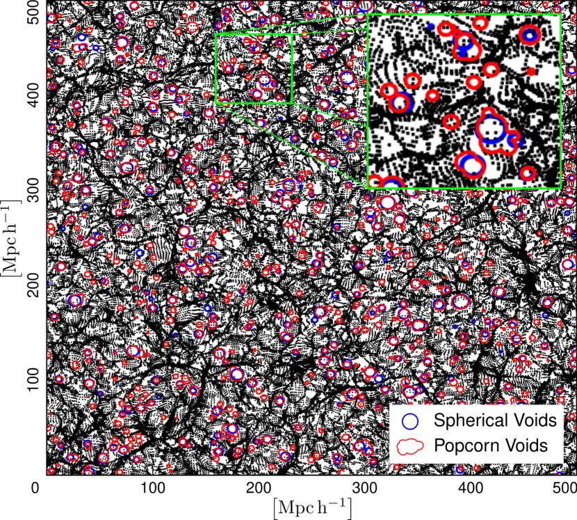
Figure 1: Slice of a dark matter-only simulation at final time (sim-1, $512^{3}$ particles in a box of $500~{}h^{-1}{\rm Mpc}$ side length). The particles (black dots) in the x-y plane have a z-coordinate between $245-255~{}h^{-1}{\rm Mpc}$. Integrated density voids (with $\Delta\leq-0.9$) were identified on the box assuming spherical (blue circles) and free-form popcorn shapes (solid red lines, see text for detailed description). These objects are shown by their intersection with the x-y plane at z$=250~{}h^{-1}{\rm Mpc}$ (solid line in red or blue).

As we briefly described in the introduction section, there are several void finders in the literature, each based on some physical characteristic of these regions. In this section we introduce a new void finder, designed to improve void abundance analyses to some extent. Roughly speaking, the basic idea behind this approach is to look for two desired features of a void object.

The first feature we look for is to obtain a definition with some kind of free form, that is, the shape of the void object must be flexible enough to fill the entire underdense region. As we will see in the following subsections, the intention here is to avoid void fragmentation, that is, to identify multiple void objects in association with a single physically significant underdense region in the large-scale distribution. This also allows us to associate a single scale to the void region, using for instance the equivalent radius of a sphere with the same volume than the void object.

The other important aspect is to identify regions that enclose a well-defined integrated density contrast. Therefore at the moment of identification the density contrast can be taken to be below some desired threshold. This parameter could be then related with a density barrier in excursion-set models at a given scale. In the following subsections, we describe in detail the popcorn void finder algorithm (Section 3.1) and its application in the dark matter distribution of $\Lambda$CDM cosmological simulations (Section 3.2). We restrict ourselves to the analysis of simulations, in this first version of the algorithm, because the periodic boundary conditions of this type of data allow us to avoid the treatment of more complicated selection functions, such as those intrinsic to galaxy surveys. In this way a popcorn object is allowed to fill an underdense region without a boundary limitation. We are leaving for future development a version of the popcorn void finder that can be run on galaxy surveys, implementing similar methods to those used in the spherical void finder on observational data (see for instance Alfaro et al., 2022; Rodríguez-Medrano et al., 2022).

Regarding the simulations in this work we analyse three boxes: sim-1, sim-2 and sim-3, with particles of $512^{3}$, $1024^{3}$ and $6720^{3}$ respectively in periodic boxes of $500$, $1000$ and $3000$ $~{}h^{-1}{\rm Mpc}$ of side length. All boxes are periodic realisations of a flat $\Lambda$CDM cosmology with the matter density and dark energy parameters given by $\Omega_{m}=0.25$, $\Omega_{\Lambda}=0.75$, respectively and a root mean square variance of linear perturbations of $\sigma_{8}=0.9$. The sim-3 box is in fact the Millennium XXL simulation (MXXL, to see details about this run please read Angulo et al., 2012).

3.1 Free form and integrated underdensity void definition

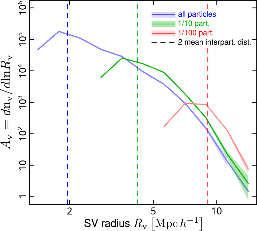
Figure 2: Abundance of spherical voids identified in the dark matter field of the sim-1 box (see Sect. 3) as a function of their radius (blue). In green and red we show the abundances when only 1/10 and 1/100 fractions of randomly selected particles are used. Shaded areas correspond to shot-noise error bars. The dashed vertical lines correspond to 2 times the mean distance between particles for these three different number densities.

In order to compute the integrated density of a given region, it is necessary to define a three dimensional boundary that defines the domain to perform such integration. We define the integrated density of a given region as the total amount of matter or tracers inside divided by its volume. In this work we distinguish this definition with respect to the most used of the differential density field, or simply the density field $\rho$, defined by $d\mathrm{M}=\rho(\mathbf{x})dV$, where $d\mathrm{M}$ is the total amount of matter in a differential volume $dV$ at a given position $\mathbf{x}$ in space. This latter scalar field can be estimated on the data using various methods, from a regular fine mesh of the simulation volume, a tessellation of the tracer distribution, or particle kernel interpolation, among others.

The popcorn void finder approach, as we will see, is a generalisation of the spherical void finder (hereafter SVF) by adding in a recursive way more spheres to fill the void region. This approach is similar to those used in the works of Colberg et al. (2005) and more recently Douglass et al. (2022), although with some differences. We start by identifying spherical voids (SV) on integrated density in the simulation box, following a procedure similar to that described in Ruiz et al. (2015). Briefly, after seeding the simulation box in regions of local low density, we place spheres in each seed and increase their radius as much as possible to keep an integrated density contrast below a certain threshold, $\Delta_{\mathrm{v}}$. After this, all overlapping spheres are removed keeping the largest ones. In this paper and in the accompanying published code, we follow a slightly different algorithm than our previous articles; however, it follows the same two main steps mentioned above. As a consequence, the spherical void samples in this new version do not change significantly from our previous results. Their abundance and distribution in space are very similar, however the new SVF provided in this work performs significantly faster and allows us to identify spherical voids in simulations with higher resolutions. For a detailed description of the method, see Appendix A. We also provide the SVF algorithm used here within the public code released along with this work.

In Fig. 1 we show a slice of the spatial distribution of dark matter particles in the sim-1 box at $z=0$. The slice depth is $5~{}h^{-1}{\rm Mpc}$, while all spherical voids found on the particle distribution and intersecting the mid-plane of the cut are shown using their intersecting circle in blue solid lines. These SV objects are defined with an integrated density contrast below the threshold of $\Delta_{\mathrm{v}}=-0.9$. On the same figure, we also over plot popcorn voids in red, as we will introduce later in this subsection. As stated before, SVs are the first step in defining popcorn objects, so it is expected that there will be at least one of these objects at every SV location.

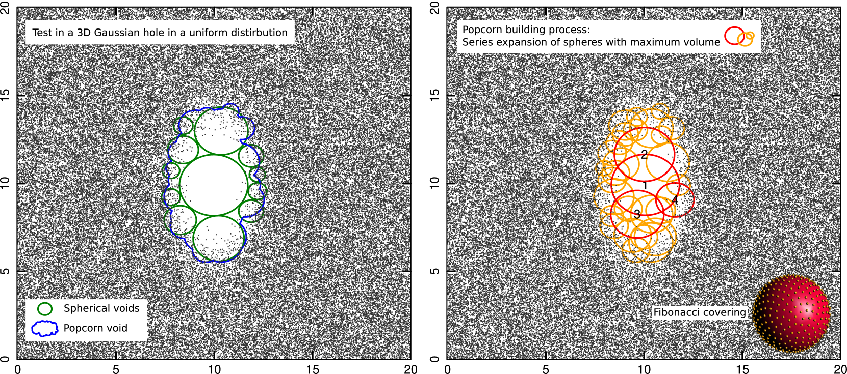
Figure 3: X-Y slice at Z$=10$ of a ellipsoidal Gaussian hole in a uniform random distribution of points in a cube of side 20 (dimensionless). Some points were drawn from the uniform box with a probability given by the product of three normal distributions over their Cartesian coordinates (see details in the text). Left panel: Spherical and popcorn void objects shown by their intersection with the midplane at Z$=10$ (green circles and solid blue curve, respectively, as indicated by the key). Right panel: The member spheres of the popcorn object (orange circles). The first 4 spheres added by the algorithm are indicated by red circles and labelled by their inclusion order. The bottom right inset is an example of a Fibonacci covering of a sphere (see the text)

The SV abundance in the sim-1 simulation as a function of sphere radius is presented in Fig. 2, in solid blue line, as defined in Eq. 1. We also present in green (red) the abundances obtained when only a particle of ten (one hundred) is used randomly chosen in the SV identification. As can be seen, void sizes tend to be larger in these random diluted samples compared to the full sample. Random particle dilution more efficiently suppresses shortwave fluctuations in the matter field, erasing small scale structures. In this way, small voids are incompletely detected and merged into larger regions. The corresponding transparent shaded areas are the error bands. We also indicate with vertical dashed lines, the scale of twice the mean interparticle distance. The behaviour of these abundances is qualitatively consistent with what we expect in a hierarchical clustering scenario: small voids outnumber larger ones, a trend similar to a Schechter function predicted by excursion-set theory. However, at radii less than a few times the mean interparticle distance, the abundance shows the opposite behaviour. This is expected due to the shot noise dominance at low density and low scale regions. This figure helps us to define what we call the shot noise radius, $R_{\mathrm{shot}}$, which is the minimum radius for which spherical voids have physical meaning (see, for instance, the analysis presented in Correa et al. (2021)). Therefore, this radius will be crucial in defining the popcorn voids.

As anticipated, the next step in the popcorn algorithm is to add more spheres to closely cover the void region. This is achieved by placing seeds on the surface of the spherical object. The seed locations follow the Fibonacci covering lattice. In an inset on the right panel of Fig. 3 we show an example of seed distribution (see the small orange dots on a red sphere). As can be seen in the figure, the seeds are placed regularly aligned on a double spiral structure on the surface of the sphere (the so called Golden Spirals). This covering scheme has some advantages over regular lattices, also being found very frequently in nature (e.g. sunflower seeds, pineapple scales, spikes in the cactus Mammillaria, see González, 2009). On the one hand, the total number of points in the scheme can be set to any odd natural number, unlike regular distributions that increase with the square (see for example Górski et al., 2005; González, 2009), this allows us to smoothly vary the number of seeds with the radius of the sphere to be covered, to ensure the desired spatial resolution (larger spheres will be more covered by seeds) The other important advantage is that the seeds in the Fibonacci lattice are optimally packed (Ridley, 1982, 1986), sampling the sphere regularly while each point has a different latitude, which allows a better sampling than regular lattices (González, 2009). This last characteristic is crucial to obtain a correct coverage of the void regions, regardless of their orientation and shape.

After covering, each seed expands one at a time, seeking its maximum radius to satisfy that the integrated density in the volume of the union of the two spheres is below the threshold, $\Delta_{\mathrm{v}}$. Then after considering each seed, the one that has expanded the most is accepted. The next step is to cover the joining surface of these two spheres, that is the surface of the initial spherical void and the accepted sphere. This is done by covering each sphere with a number of seeds appropriate to its size and the desired spatial resolution, and not considering those seeds that fall inside any sphere. Then the process of seeding, keeping only the most expanded sphere, and seeding again is repeated iteratively. Thus, in the second step, the most expansive seed in the joint volume of three spheres is accepted, and in subsequent steps the volume of the union of four, five spheres, is taken into account. The process ends once no sphere with a radius greater than a given threshold $R_{\mathrm{th}}$ can be added, satisfying the integrated density contrast condition ($\Delta<\Delta_{\mathrm{v}}$). This radius threshold is chosen as the radius of the shot noise, $R_{\mathrm{th}}=R_{\mathrm{shot}}$.

In this way it can be deduced that the measurement of $R_{\mathrm{shot}}$ is fundamental for the definition of a popcorn object. $R_{\mathrm{th}}$ can be defined a priori as a few times the mean interparticle distance or it can be chosen more precisely as the radius where the behaviour SV abundance change. That is, $R_{\mathrm{shot}}$ can be defined as the scale at which the SV abundance departs from a power law with negative slope. We have found that if spheres with radius smaller than $R_{\mathrm{shot}}$ are allowed, artificially large void objects are obtained, with a complex multiconnected topology. As a side effect, the total computation time becomes significantly longer. On the other hand, a large value of this threshold ($R_{\mathrm{th}}>R_{\mathrm{shot}}$) results in artificially fragmented voids, that is multiple objects associated to a single underdense region, and at small scales popcorn objects are identical to their associated spherical void.

In Fig. 4 we show the abundances of spherical voids (blue) and popcorn voids for two different values of $R_{\mathrm{th}}$ (red and green) identified over the sim-2 particle distribution at $z=0$. In an analogous way to the case of spherical voids, the VSF defined in Eq. (1) is generalised to popcorn voids by replacing the sphere radius by an equivalent radius defined as the radius of a sphere $R_{\mathrm{v}}$ of equivalent volume to that of the popcorn void ($V_{\mathrm{v}}$),that is:

$$R_{\mathrm{v}}=\left(\frac{3\,V_{\mathrm{v}}}{4\pi}\right)^{1/3}$$ (7)

The shaded areas in Fig. 4 correspond to one standard deviation around the measurements. The solid green line is the abundance of popcorn objects obtained using a larger than ideal threshold radius, that is $R_{\mathrm{shot}}<R_{\mathrm{th}}=5~{}h^{-1}{\rm Mpc}$. In this case, the abundance of popcorn objects closely matches that of spherical ones up to $R_{\mathrm{th}}$, as expected by definition. After this scale, the abundance shows a behaviour different from that expected from the abundance models, having an inflection point close to the chosen threshold radius. The solid red line corresponds to the abundance of popcorn voids with $R_{\mathrm{th}}=R_{\mathrm{shot}}$. The abundance of these objects behaves qualitative similar to what is expected for the theory. However as can be seen in the figure, their abundance is by far underpredicted by the excursion-set models of Jennings et al. (2013) (Vdn), when a linear density barrier of $\Delta_{\rm v}^{\rm L}=-5.16$ is used, that is, the corresponding value on the spherical evolution model for a non-linear density threshold of $\Delta_{\mathrm{v}}=-0.9$ (similar behaviour is obtained using $\Delta_{\mathrm{v}}=-0.8$). In the next section we will return to these results and their comparison with theoretical predictions of void abundances. Finally, after running the iterative process described above for each SV, all overlapping popcorn candidates, with an intersecting volume larger than the volume of the shot noise sphere ($4\pi/3R_{\mathrm{shot}}^{3}$), are removed starting with those with the smallest initial SV and keeping those with the larger initial SV.

The popcorn void finder algorithm can be summarised in the following recipe:

a) Seed regions of local low density and grow spheres to the largest radius allowed by $\Delta<\Delta_{\mathrm{v}}$.

b) Remove all overlapping spheres starting with the smallest ones and keeping the largest ones. In this step, a catalogue of spherical voids is produced, each of which is taken as a popcorn candidate.

c) Cover regularly the surface of the popcorn candidate with seeds.

d) Expand each seed to the largest radius that the condition $\Delta<\Delta_{\mathrm{v}}$ allows in the joint volume of the candidate popcorn and the tested sphere.

e) The seed that expands the most and has a radius greater than $R_{\mathrm{shot}}$ is accepted and the current popcorn candidate is updated.

f) The process is repeated iteratively from step c) until no sphere can be added to the candidate.

g) All intersecting popcorn objects are removed, tolerating volume intersections lower than the shot noise limit, starting with the candidate with the smallest initial SV and keeping those with larger initial SV.

In Fig. 3 we present an illustrative example of the application of the method described above. In a three-dimensional uniform random distribution of points, we have eliminated some of them according to a 3D multivariate normal distribution. The three joint Gaussian probabilities of this distribution have the same mean, that is, the coordinates of the centre of the box and different second moments. In this way we have obtained a kind of triaxial Gaussian hole, as can be seen in the slice shown in the figure. This toy data set allowed us to test some aspects of the popcorn algorithm as we designed it. In the right panel of Fig. 3 we show a section of the spherical members of the resulting popcorn after the step g (solid orange and red lines). The red circles correspond to a slice of the spheres added in the first four iterations of the algorithm, in the order labelled by the numbers in the figure. In blue on the left we show the corresponding intersection of the popcorn surface and with green circles the identified spherical voids. This is a simple example of void region fragmentation when using a spherical void finder. As we will see in the following sections, this is an important aspect in exploiting void abundances as cosmological tests. In this data set, the regions of maximum volume below any density threshold are, by definition, ellipsoids at the centre of the box with semi-axes proportional to the second moment of the Gaussian distributions. The integrated density contrast in these ellipsoids can be derived using the corresponding error functions of the three axes. We have also tested the effect of the angular orientation of the multivariate distribution on the void finder results. Regarding volume estimation, we have found that the popcorn void finder converges uniformly to the expected values depending on the minimum allowed sphere size and also on the numerical density of random points. This convergence is faster using the Fibonacci covering scheme than the regular seed distribution for all orientations.

To improve the clarity of the above description of the popcorn void finder, a non-trivial technicality has been delayed until now. To the authors’ knowledge, there are no simple analytical formulas for the joint volume of more than three spheres. The popcorn algorithm requires thousands of volume calculations of arbitrary distributions of spheres in the assembly of each popcorn candidate. Calculation of volumes by Monte Carlo methods is not feasible here due to computation time and numerical precision required. The problem of calculating the joint volume of a union of spheres is a well-known problem in the field of Chemical Physics. For instance, the estimation of the solvation energy of proteins usually requires calculation of the surface area and volume of macromolecules, which are modeled as the superposition of a large number of spheres (atoms). The arvo (Buša et al., 2005; Buša et al., 2012) package solves this problem through an extremely efficient analytical approach, calculating the surface area and volume of arbitrary sets of overlapping spheres with high precision. We use the C version of the library provided by the authors of this software.

In this subsection, we have provided a full description of the algorithm used in the definition of popcorn voids; for more details, the interested reader can review the documentation and source code provided on https://gitlab.com/dante.paz/popcorn_void_finder. In the next subsection we provide some examples of the application of this new void finder in numerical simulations.

3.2 Popcorn void properties on matter field

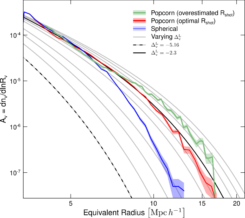
Figure 4: Abundance of popcorn voids identified in the dark matter particle field as a function of their equivalent radius. The results are shown for two different values of $R_{\mathrm{th}}$: in red when this parameter is equal to the radius of the shot noise, and in green when a larger value is used. The abundances of spherical voids are shown in blue. The shaded areas correspond to the uncertainties of the shot noise. Solid gray, solid black, and dashed black lines correspond to different Vdn excursion-set models with varying linear density barrier values.

As presented in the previous subsection, Fig. 4 shows the abundance of popcorn voids identified in dark matter particles in $\Lambda$CDM simulations (solid red line). As we mentioned before, the solid blue line corresponds to spherical voids. As can be seen, spherical voids at the small size end have higher abundances than the models, while the opposite is observed for large radii. This is probably due to the fragmentation problem of spherical void finders when identifying void regions. The black dashed line in the figure represents the predicted void abundance using the Vdn model with a linear density barrier of $\Delta_{\mathrm{v}}^{\mathrm{L}}=-5.16$, which corresponds to an integrated nonlinear density contrast of $\Delta_{\mathrm{v}}=-0.9$ in the spherical expansion model (See Sect. 2). As can be seen, this prediction significantly underestimates the abundance of spherical and popcorn voids with this specific equivalent integrated density contrast in the simulation box. The solid grey lines depict the results of the Vdn model using different values of $\Delta_{\mathrm{v}}^{\mathrm{L}}$. Notably, a value close to $\Delta_{\mathrm{v}}^{\mathrm{L}}=-2.3$ provides a good fit to the popcorn abundances. Note that no feasible value of the linear density barrier can be found to obtain a reasonable fit for the spherical void sample. On the other hand, when the same experiment is conducted using the SvdW model, the predicted abundances show a steeper slope and vary much more rapidly (results not shown for brevity) and those model results cannot be reconciled with the abundances of spherical or popcorn voids for any value of $\Delta_{\mathrm{v}}^{\mathrm{L}}$. Similar results are obtained when identifying spherical and popcorn voids using a nonlinear density contrast of $\Delta_{v}=-0.8$. For this threshold, the spherical evolution model provides a linear density contrast barrier of $\Delta_{\mathrm{v}}^{\mathrm{L}}=-2.8$, which leads to a significant underestimation of the abundances once again. However, we find that a better fit to the popcorn abundances can be achieved using a higher value of density barrier (in this case, $\Delta_{\mathrm{v}}^{\mathrm{L}}=-1.3$).

Since the abundance models fail to reconcile the observed spherical void abundances, we can infer that popcorn voids may be more suitable for studying abundances. As we anticipated when analysing the simply test presented in Fig. 3, the identification using free-form integrated densities allows a more complete coverage of the void regions. This seems to have two effects on the abundance of voids, on the one hand it alleviates the overabundance of small voids in fragmented regions, while also allowing a better characterisation of the scale associated with large voids. It is important to note that here the size of the popcorn object is defined by its volume, i.e. its equivalent radius, and this scale is assumed to be comparable to the radius scale used in excursion-set theory. This approach is different from that used in Jennings et al. (2013) and Marulli et al. (2016), where the voids identified in the density field are associated with the largest integrated density sphere within the void object.

It is worth to emphasise that popcorn void abundances can be modelled by using higher values of the linear density barrier, rather than those expected in the spherical expansion model. These deviations from the spherical expansion model may be due to various factors, including deviations from the isolation assumption. The non-spherical nature of void regions arises from their interaction with other structures (see for instance Ceccarelli et al., 2016). Furthermore, any differences between the nonlinear evolution predicted by the spherical model and the dynamics of voids observed in the numerical simulation could also contribute to these deviations in the relation between $\Delta_{\mathrm{v}}^{\mathrm{L}}$ and $\Delta_{\mathrm{v}}$. Additionally to this last parameter, the VSF models are dependent also on cosmological parameters and the critical density for collapsing objects (here we adopt $\Delta_{c}=1.6$).

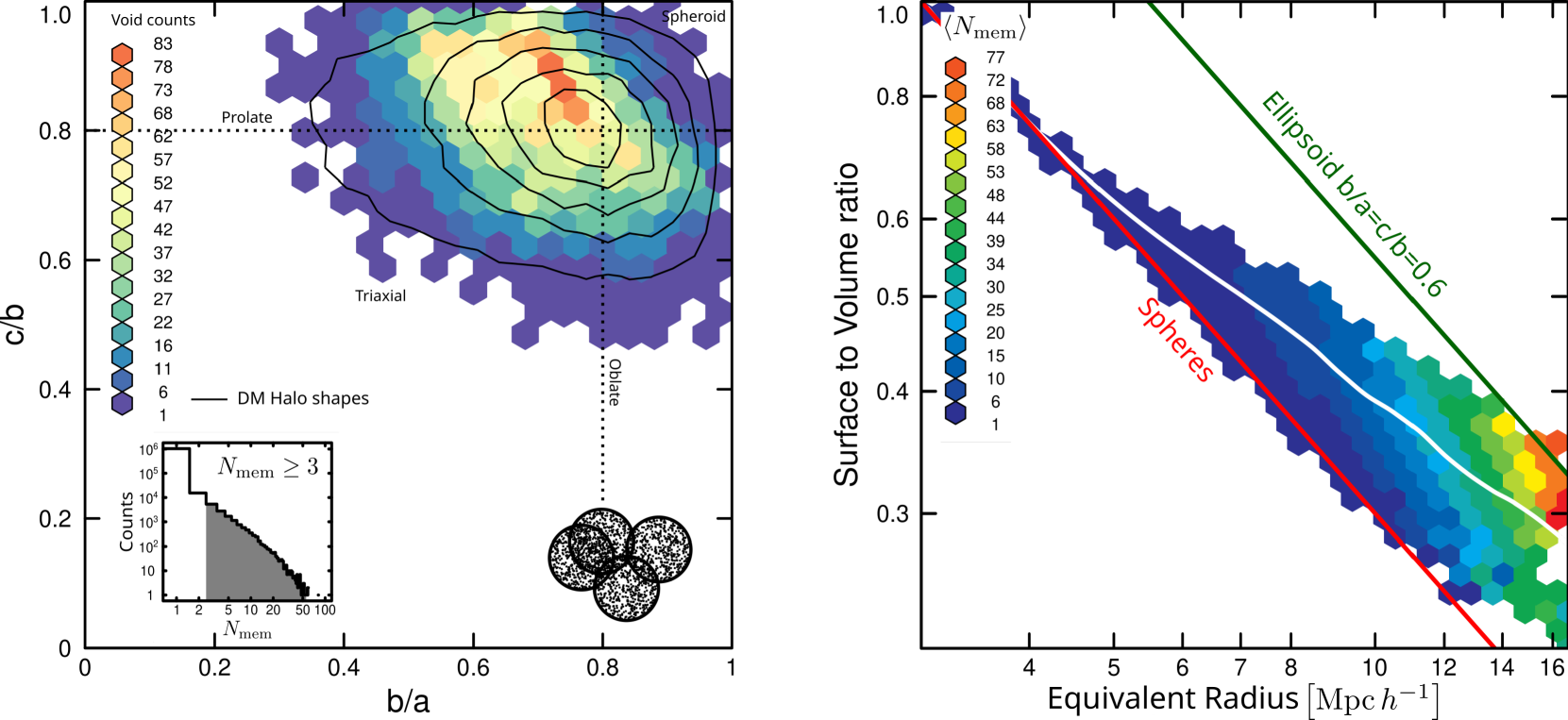
Figure 5: Left panel: Distribution of popcorn objects with three or more member spheres ($N_{\mathrm{mem}}\geq 3$) according to the length ratio of the semi-axes of the void shape, b/a and c/b. The number of objects in each hexagonal bin is indicated by the colours (see the bar on the left). Solid line black contours show the distribution of Dark Matter halo shapes ($\mathrm{M}_{\mathrm{halo}}\geq 10^{12}~{}h^{-1}{\rm M_{\odot}}$, see Paz et al., 2006). The bottom left box is a histogram of the number of member spheres per void, while the grey shaded area corresponds to the sample in the left panel of the figure. Right panel: Mean number of spherical members of popcorn voids $\langle N_{\mathrm{mem}}\rangle$ in hexagonal bins of equivalent radius and ratio of surface area to volume. Both axes are in logarithmic scale, the red and green solid lines correspond to the expected surface area to volume ratios for spheres and triaxial ellipsoids with b/a = c/b = $0.6$ as a function of their size. The solid white line corresponds to the void average behaviour.

In Fig. 5, we present an analysis of the shape, volume, and surface of the popcorn objects identified in the matter field of sim-2. In the case of the shape analysis, we use popcorn voids with three or more member spheres ($N_{\mathrm{mem}}\geq 3$). As described above (see Section 3), the arvo library provides the surface area and volume of the union of spheres using an analytical approach. To analyse the shape of the popcorn objects, we calculate the shape tensor of the region defined by the union of the member spheres using a Monte Carlo approach. Inside each sphere, we randomly allocate $N_{\mathrm{ran}}$ points, assigning each one a weight or mass, $m_{\mathrm{k}}$, given by the inverse of the number of intersecting spheres at its location, that is $1/N_{\mathrm{sph}}({x_{1}}^{\mathrm{k}},{x_{2}}^{\mathrm{k}},{x_{3}}^{\mathrm{k}})$ (where the location of the point is expressed through its Cartesian coordinates). An example of such a random set in a popcorn void is shown in the lower right schematic drawing in the left panel of Fig. 5. This set of $N_{t}=N_{\mathrm{ran}}N_{\mathrm{mem}}$ random points weighted in this way is equivalent to a uniform mass distribution within the volume of the popcorn. We define then a Monte Carlo estimate of the shape tensor of the region as:

$$I_{\mathrm{ij}}:=\frac{1}{N_{t}}\sum_{\mathrm{k=0}}^{N_{t}}m_{\mathrm{k}}\left({x_{\mathrm{i}}}^{\mathrm{k}}-\bar{x}_{\mathrm{i}}\right)\left({x_{\mathrm{j}}}^{\mathrm{k}}-\bar{x}_{\mathrm{j}}\right)$$ (8)

where $\bar{x}_{\mathrm{i}}$ are the components of the geometric centre of the region:

$$\bar{x}_{\mathrm{i}}:=\frac{1}{N_{t}}\sum_{\mathrm{k=0}}^{N_{t}}m_{\mathrm{k}}{x_{\mathrm{i}}}^{\mathrm{k}}\,.$$

The eigenvalues of this tensor are the square of the lengths of the semiaxes (a, b, c with, a$\geq$b$\geq$c) of the characteristic ellipsoid that best approximates the popcorn volume. The b/a and c/b quotients allow us an analysis of the ellipsoidal figures of best fit (see for example Frenk et al., 1988; Paz et al., 2006; Gonzalez et al., 2021; Gu et al., 2022, and their references) of the objects and their classification in spheroids (b/a$\simeq$c/b$\simeq 1$), prolate type (i.e. elongated, 1$\simeq$c/b>b/a), oblate type (i.e flattened 1$\simeq$b/a>c/b) and triaxial (similar ratio between semiaxes lengths, b/a$\simeq$c/b). As can be seen from the above reference list of previous works, this type of shape analysis has been widely applied in the analysis of dark matter haloes, galaxy groups, and galaxy cluster shapes.

In the left panel of Fig. 5, we include with solid black lines the isocontours of the shape distribution for dark matter haloes with masses greater than $10^{12}~{}h^{-1}{\rm M_{\odot}}$ as presented in Paz et al. (2006). In that work we present an extensive analysis of the effect of shot noise in the determination of halo and galaxy group shapes using shape tensors. In our case, shot noise is not an issue due to the large number of random points used, however we are limited by the number of member spheres of each popcorn object ($N_{\mathrm{mem}}$). Popcorn voids with only one sphere are, by definition, in the upper right corner of this figure, while objects with only two spheres are, by definition, perfect prolate ellipsoids (collapsed on the axis given by c/b$=1$). The number of member spheres follows a power law distribution (see lower left inset of the left panel of Fig. 5) and more than $98\%$ of the objects have only one or two member spheres, being mostly small objects ($95\%$ have sizes below $7~{}h^{-1}{\rm Mpc}$). Given a total sample of 1065912 popcorn objects identified in sim-2, 1051176 voids have one or two member spheres, while 14736 objects have three or more member spheres (grey shaded area in the figure inset). We restrict the shape analysis to those popcorn voids that have three or more members. With dotted lines at b/a$=0.8$ and c/b$=0.8$, we have divided the space of the axis ratios into four regions, as indicated in the figure: spheroidal, prolate-like, oblate-like, and triaxial. As can be seen, the peak of the shape distribution of void regions lays in the prolate region of the diagram. Compared to halo shapes, voids exhibit a similar behaviour, presenting mostly triaxial shapes with a prolate trend, more pronounced in void than in dark matter haloes.

In the right panel of Fig. 5, we show the mean number of sphere members in hexagonal bins of equivalent radius and ratio of surface area to volume. The surface area to volume ratio (usually indicated as sa/vol or SA:V in chemistry and physics) can give us an idea of the compactness of popcorn shapes. The red line corresponds to the sa/vol ratio of spheres as a function of their radius, that is, a power law with index -1 (for spheres sa/vol$=3/R_{\mathrm{v}}$). In the case of triaxial ellipsoids, similar behaviours are obtained, almost the same index but with different numerical factors, that is, a straight line parallel to sa/vol of spheres in the log-log space of the figure. An extreme case seems to be the triaxial ellipsoid with b/a=c/b=0.6, whose sa/vol ratio is indicated by a solid green line. The behaviour of popcorn objects seems to follow an intermediate behaviour between spheres and triaxial ellipsoids. This fact can be understood as an indication that the topology of popcorn voids is somewhat close to their ellipsoidal figures of best fit. A complex behaviour or a different compactness of popcorn regions compared to ellipsoids should result in quite different sa/vol ratios as a function of size, and not the intermediate behaviour displayed in the figure. The trend of the average number of spherical members in the hexagonal binning scheme of the figure (the visible colour gradient), seems to indicate that depending on the number of members, the sa/vol ratio behaves like ellipsoids with increasing axis ratio.

4 Cosmological test using Void abundances

In this section we present an analysis of the void abundances measured in a biased tracer field. More specifically, we study the void size function (VSF) of identified objects in the distribution of dark matter haloes and how this function depends on cosmology and redshift-space distortions. We also show how the modelling presented in Correa et al. (2021) to account for geometric and redshift space distortions on abundances of spherical voids can also be applied in our context of integrated density free-form voids. As in that previous work, we define geometric distortions (GD) as those that arise when assuming a fiducial cosmology (but different from the underlying one) when transforming coordinate measurements (position angles and redshifts) to comoving coordinates. This is the concept behind any AP test, if an object is assumed to be the same physical length along the line of sight (LOS) and in the plane of the sky (POS), any distortion that produces a change in the aspect ratio between these directions can be used to derive the underlying cosmological parameters. For further details the interested reader can see Section 2 of Correa et al. (2019). On the other hand, the peculiar velocities introduce deviations in the estimation of the distances to galaxies by using the Hubble’s law. These redshfit space distortions (RSDs) in expanding voids result in apparently larger void regions relative to their size in the underlying three-dimensional space (see Correa et al., 2021, and references there in). Finally, combining the correction factors derived by Correa et al. (2021) with excursion-set theory models of the VSF, we present a cosmological test applicable to the abundance of voids identified in the biased tracer field in redshift space.

4.1 Abundance of voids in biased tracer field and Alcock-Paczyński distortions

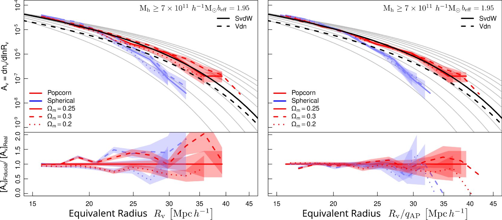
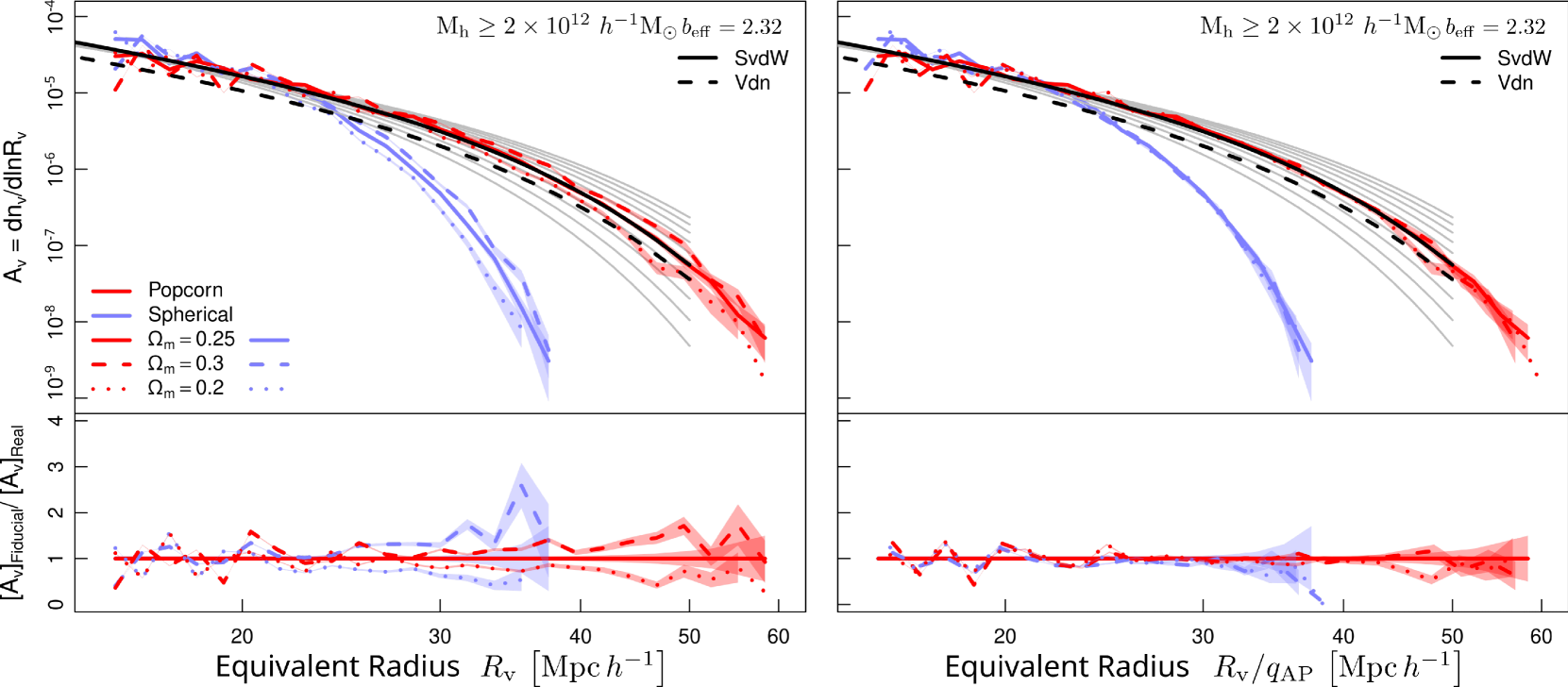
Figure 6: Left panels: Abundance of spherical voids (solid blue line) and popcorn voids (solid red line) identified using the real-space position of dark matter haloes with masses greater than $7\times 10^{11}~{}h^{-1}{\rm M_{\odot}}$ (upper panels) and $2\times 10^{12}~{}h^{-1}{\rm M_{\odot}}$ (lower panels) at $z=0.51$ as a function of the equivalent radius ($\mathrm{A}_{\mathrm{v}}$). The dashed (dotted) line corresponds to the voids identified in the boxes with a higher (lower) value of the matter density parameter in the assumed fiducial cosmology. In each panel, the quotient between the abundances in fiducial and real cosmology is shown below. Right panels: The void abundances corresponding to the left panels as a function of the equivalent void radius corrected for geometric distortions with the factor $q_{\rm AP}$ as defined in the text.

In the left panels in Fig. 6, we show the abundance of spherical voids (blue solid line) and popcorn voids (red solid line) identified using the real-space position of dark matter haloes at $z=0.51$. Haloes were taken as tracers from two simulation boxes, sim-2 and sim-3, with masses in the range of $M_{\rm halo}\geq 7\times 10^{11}~{}h^{-1}{\rm M_{\odot}}$ and $M_{\rm halo}\geq 2\times 10^{12}~{}h^{-1}{\rm M_{\odot}}$ (top and bottom panels, as indicated in the figure key). Similar results are obtained using different halo mass cuts in both simulation boxes. Using the same colour code (blue for SV and red for popcorn voids) with dashed and dotted lines, we show the corresponding abundance of objects identified in boxes with a different fiducial cosmology than the underlying one. In detail, the dotted and dashed line correspond to the abundances obtained when the halo coordinates are transformed from true position to angles and redshifts, assuming a true cosmology, and then immediately transformed back to comoving space, but this time assuming a fiducial cosmology with a lower or higher value of $\Omega_{\mathrm{m}}$. For this procedure we assume a distant observer and a mean redshift of $z=0.51$. This transformation of coordinates from real space to observable space and then back to a comoving space but assuming an incorrect cosmology introduces a pattern of distortion (GD) in the relative distances along the POS and LOS directions from the point of view of the observer (for a detailed description of geometric distortions see Correa et al., 2019, 2021). The void size functions on the right panels of Fig. 6 take the same ordinate values as those on the left, but their arguments (the abscissas $R_{\mathrm{v}}$) are corrected of GD by dividing them by the following factor (as derived in Correa et al., 2021):

$$q_{\rm AP}=\sqrt[3]{\left(\frac{D_{\rm M}^{\rm fid}(z)}{D_{\rm M}^{\rm true}(z)}\right)^{2}\frac{H_{\rm true}(z)}{H_{\rm fid}(z)}}.$$ (9)

As can be seen, the $q_{\rm AP}$ factor correctly captures the effect of geometric distortion of void sizes. It depends on the comoving angular diameter distance at the sample mean redshift ($z$) in the fiducial and underlying cosmologies, $D_{\rm M}^{\rm fid}$ and $D_{\rm M}^{\rm true}(z)$, respectively, as well as in the Hubble parameter for both cosmologies, i.e. $H_{\rm true}$ and $H_{\rm fid}$. It is not surprising that the same factor can correct the volumes of spherical and free-form voids, since geometric distortions at a given fixed mean redshift take the form of a linear coordinate transformation and $q_{\rm AP}$ is its Jacobian determinant.

In Fig. 6 we also include in all panels the corresponding results of the excursion-set models of Jennings et al. (2013) and Sheth & van de Weygaert (2004) using thick dashed and solid black lines, labeled as Vdn and SvdW in the figure key, respectively. As was introduced in Sect. 2, to predict void abundance, it is necessary to convert the integrated density threshold used in void identification (for both spherical and popcorn voids) from $\Delta_{\mathrm{v,g}}=-0.9$ over the tracer sample to a density threshold in the matter field by means of a bias factor, ie $\Delta=\Delta_{\mathrm{v,g}}/b_{\mathrm{eff}}$ (as described in Ronconi & Marulli, 2017). The bias factors $b_{\mathrm{eff}}=1.95$ and $b_{\mathrm{eff}}=2.32$ have been used for the low and high mass halo samples, respectively (upper and lower panels as indicated in Fig. 6) to fit the results.

As can be seen, in this case of biased tracer samples, the model that best fits the simulation data is the SvdW. By definition, the Vdn model always predicts a lower amplitude at small scales than SvdW (and consequently lower than simulation data) due to the volume fraction conservation constraint, regardless of the tracer bias used. This differs from the results on abundances in the matter field presented in Section 3 and may be related with an effect of tracer bias on the volume conservation constraint assumed in the Vdn model. In addition, the reduction in the number of tracers may be affecting void sizes in a similar manner to the shot noise effect illustrated in Figure 2, however, this effect may be compounded with the tracer bias. In the Jennings et al. (2013) work, the authors also compare the abundances predicted by the Vdn model with void objects obtained from a different void finder than the one used here. Despite this, they also find discrepancies between the model and the data. As these authors explain, this problem may be related to the fact that the voids identified in the halo samples are not simply related to the void samples identified in matter, a fact that is common to all void finders. A one-to-one relationship between halo voids and matter voids is not feasible, the time evolution of halo voids depends on the definition of the halo sample (the mass cut for instance). Based on halo mass and assembly history, a void defined in a given halo tracer field at a given redshift does not uniquely correlate with a precursor void at an earlier time. In this work, we simply apply the abundance models (Vdn and SvdW) by transforming the nonlinear void density contrast threshold (used in the popcorn identification) in the halo field to an equivalent value in the matter field through a free bias parameter, used to fit the data. It is important to note that this bias parameter is also encoding by definition possible deviations in the spherical expansion model, as was described in section 3.2. Our goal is to find a suitable model for the inference of cosmological parameters from the abundance of popcorn voids. Although it would be very important to have an adapted model for voids identified in biased tracer samples, we define this issue as outside the scope of this work.

Going back to the results in Fig. 6, at small sizes and regardless of the assumed bias, the SvdW model better predicts void abundance for both spherical and popcorn objects. The solid grey lines in the figure correspond to $0.1$ variations in the bias factors, from $b_{\mathrm{eff}}-0.5$ to $b_{\mathrm{eff}}+0.5$. As we mentioned before and can be seen in the figure, the abundances at small radii are insensitive to the assumed bias (as it is mentioned in Jennings et al., 2013). On the other hand, the behaviour of the VSF models at large sizes seems incompatible with the abundance of spherical voids. In contrast, the SvdW model fits well with the abundance of popcorn objects for a proper bias parameter. It is important to emphasise the fact that here the bias factor is used as a nuisance fitting parameter and is not necessarily related to the bias factor between the clustering measures, or between matter and halo velocity fields. For the halo samples analyzed in this section, namely those with $M_{\rm halo}\geq 7\times 10^{11}~{}h^{-1}{\rm M_{\odot}}$ and $M_{\rm halo}\geq 2\times 10^{12}~{}h^{-1}{\rm M_{\odot}}$, the expected values of the clustering bias at $z=0.51$ are $0.91$ and $1.05$, respectively, as computed using the formulae presented in Tinker et al. (2010). As can be seen, these values for clustering bias are much smaller than the corresponding best-fit $b_{\rm eff}$ values. We see larger differences between the effective bias required to fit popcorn abundances and the clustering bias compared to similar studies using other void finders (Contarini et al., 2019; Pollina et al., 2017; Pollina et al., 2019). The question of tracer bias around void regions remains open and is an active research topic. For further information, we recommend also reading the following works: Chan et al. (2019); Fang et al. (2019); Chan et al. (2014); Schuster et al. (2019); Chan et al. (2020).

4.2 Model fitting of void abundances in redshfit space

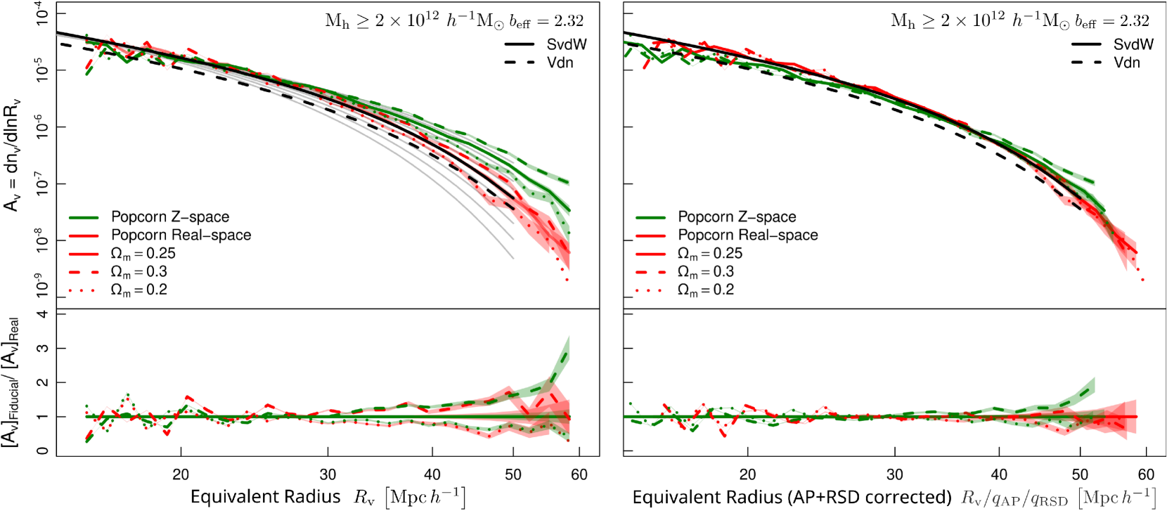
Figure 7: Left panel: Abundance of popcorn voids in real and redshift space, solid red and green lines, respectively, identified on dark matter haloes with masses greater than $2\times 10^{12}~{}h^{-1}{\rm M_{\odot}}$ at $z=0.51$ as a function of the equivalent radius ($\mathrm{A}_{\mathrm{v}}$). The dashed (dotted) line corresponds to the voids identified in the boxes with a higher (lower) value of the density parameter in the assumed fiducial cosmology. The quotient between the abundances in fiducial and real cosmology is shown below. Right panel: The void abundances corresponding to the left panels as a function of the equivalent void radius corrected for geometric and redshift-space distortions with the $q_{\rm AP}$ and $q_{\rm RSD}$ factors as defined in the text.

So far, we have addressed the effect of geometric distortions (the Alcock-Paczyński effect) and tracer bias on void abundance, now we will check if the treatment of redshift-space distortions presented in Correa et al. (2021) can be applied in the context of popcorn voids. In an analysis similar to that presented in our previous works, using the distant observer approach, we add the peculiar velocity component in the LOS direction as an additional Doppler term to the cosmic redshift. This introduces a redshift-space distortion (RSD) pattern at the halo positions (see for example Paz et al., 2013). Being voids regions of negative density contrast a positive divergence of the velocity field is expected, and thus the apparent position of the tracer haloes in redshift space is shifted toward the outskirts of the void. Therefore, the size of voids identified in redshift surveys tend to be larger than in real space, resulting in a right-shifted VSF along the $R_{\mathrm{v}}$ axis.

In Correa et al. (2021) we have derived a correction factor for the RSD in the radius of spherical voids from linear theory:

$$q_{\rm RSD}=1-\frac{1}{3}\delta R_{\rm v}\beta(z)\Delta_{\mathrm{v,g}}.$$ (10)

where ${\beta}$ is the growth rate of structures over a bias factor (see for instance Paz et al., 2013; Hamaus et al., 2015, and references there in) and $\delta R_{\rm v}$ is a parameter to quantify the variation on the predicted expansion of the void radius. This factor is derived from the expected expansion of a hypothetical underdense spherical region, of radius $R_{\mathrm{v}}$, due to RSD. In that context, the elongation produced by RSD along LOS distorts this sphere into an ellipsoid in redshift space, with a major semi-axis greater than $R_{\mathrm{v}}$ and intermediate and minor semi-axes equal to $R_{\mathrm{v}}$. When a spherical void finder is used, this region is associated with a spherical void object with a radius between the semi-major axis and the radius in real space. Therefore, the derivation of a theoretical value of $\delta R_{\rm v}$ will depend on the details of the spherical void profile around the scale associated with the integrated density threshold ($\Delta_{\mathrm{v,g}}$). In Correa et al. (2021) we have derived for spherical voids a mean value of $\delta R_{\rm v}$ between $0.5$ and $0.3$, depending on the size of the void. However, it is important to stress the fact that in the case of popcorn voids we have chosen to study its abundances as a function of its equivalent radius, that is the radius of the sphere with a volume equivalent to the one of the identified object. In this work we will correct the equivalent popcorn void radius by dividing it with the $q_{\rm RSD}$ factor defined in Eq. (10). However, the interpretation of the role of $\delta R_{\rm v}$ has to be different. The popcorn void finder is designed to define free-form objects, so a void region can be considered to a first approximation as an ellipsoidal region, with an arbitrary orientation, assumed to be uniform due to cosmic isotropy. It can be assumed that the shape parameters of these regions follow the distributions shown in Fig. 5. In the context of popcorn voids, $\delta R_{\mathrm{v}}$ depends on the orientation of the void, the details of the velocity field around the void region (not necessarily well described by the model of spherical linear expansion) and the average of the different shapes in a bin of equivalent radius. In this work, $\delta R_{\rm v}$ will be used as a free parameter to adjust the RSD of the popcorn void sizes.

Since $\beta$ is a parameter defined in the spherical expansion model, we derive it from spherical voids, following the same procedure as in Correa et al. (2019) and Correa et al. (2021). In a tracer sample of haloes with masses greater than $2\times 10^{12}~{}h^{-1}{\rm M_{\odot}}$ at $z=0.51$, we have measured the radial velocity and density profiles of spherical voids, finding a $\beta$ value of $0.54$ in a range of sizes from $15$ to $40~{}h^{-1}{\rm Mpc}$. As we will see below, popcorn voids are well characterised with an RSD parameter of $q_{\rm RSD}=1.12$, which corresponds to an increase in radius of $\delta R_{\mathrm{v}}=0.74$.

In Fig. 7 we show the abundance of popcorn voids in real space (solid red lines) and redshift space (solid green line) identified using dark matter haloes with masses greater than $2\times 10^{12}~{}h^{-1}{\rm M_{\odot}}$ at $z=0.51$. In the left panel, the abundances are shown as a function of the equivalent radius of the void (as defined by Eq. 7) calculated from the volume of popcorn objects identified in real or redshift space, depending on the case considered. As in the previous analysis, dashed and dotted lines correspond to voids identified after the coordinates of each halo are affected by geometric and redshfit distortions. This is done by transforming halo coordinates from real to observable space, using the simulation’s underlying cosmology, adding a component of Doppler shift along the LOS, and finally transformed back to comoving space but using a fiducial cosmology with a different value of the density parameter. The quotient between abundances in fiducial and real cosmology is shown in the bottom plot of each panel. In the right panel we show the abundance of popcorn objects once their volumes are divided by the correction factors $q_{\rm AP}$ and $q_{\rm RSD}$. The shaded areas correspond to Possion noise standard deviations. As can be seen the application of both factors successfully correct the void size functions from geometric and redshift-space distortions. The abundances shown in the right panel of Fig. 7 are indistinguishable in almost all scales, showing marginally differences between them at large sizes ($R_{\mathrm{v}}>40~{}h^{-1}{\rm Mpc}$), where the cosmic variance is more important. As in the Fig. 6, the SvdW model with a bias factor of $2.32$ seems to be good fit.

So far we have described how to correct void abundance measurements for redshift space distortions and how to model the Alcock-Paczyński effect. We have also shown a good apparent concordance of these measurements with excursion-set models, after applying the appropriate corrections. Now we will analyse the model fit statistics, in particular the combination of excursion-set models with the factors $q_{\rm RSD}$ and $q_{\rm AP}$ to obtain information on cosmological parameters. We will limit ourselves to the matter density parameter and the root mean square variance of linear perturbations to show the potential of the abundance of voids as cosmological test, leaving the analysis of a larger parameter space for future work. In Fig. 8, we show the likelihood function for the evaluation of the SvdW model for the abundance of popcorn voids. As above, the voids are identified using haloes in redshift space and assuming a fiducial cosmology, in this case with a lower value of the matter density parameter, i.e. the dotted curves shown in Fig. 7. Identical results are obtained using higher values of the density parameter, indicating that the test appears to be independent of the assumed fiducial cosmology.

The parameter space explored consists of the matter density parameter $\Omega_{\mathrm{m}}$, the root mean square variance of linear fluctuations at $8~{}h^{-1}{\rm Mpc}$ $\sigma_{8}$, an effective bias $b_{\mathrm{eff}}$, and the correction factor of redshift-space distortions $q_{\rm RSD}$. The effective bias is used to convert the halo density contrast threshold used in popcorn identification, $\Delta_{\mathrm{v}}=-0.9$, to an equivalent nonlinear density contrast in the matter field, i.e. $\Delta_{\mathrm{NL}}=\Delta_{\mathrm{v}}/b_{\mathrm{eff}}$. This value is then transformed into a linear value by means of the fitting formula presented in Bernardeau (1994, , see Sect. 2). In this way, the linear density contrast in the matter field, $\Delta_{\mathrm{L}}$, corresponding to the density threshold used in void identification, is used as the void density barrier in the excursion-set models. See Sec. 2 for more details. The matter density parameter plays a role in the evaluation of excursion-set models (through the matter spectrum in the barrier statistics) and in the factor $q_{\rm AP}$. The value $\sigma_{8}$ determines the amplitude of the power spectrum that then directly impacts the VSF. Finally, we have chosen to fit the factor $q_{\rm RSD}$ instead of $\delta R_{\mathrm{v}}$ to decouple the bias factor in the velocity field (which appears in the definition of $\beta$, Eq. 10) from the effective bias ($b_{\mathrm{eff}}$) used in the computation of the density barrier in the SvdW model. The measurement of the bias in the velocity field by means of the velocity curves of spherical voids as presented before, gives us inconsistent values of beta with $b_{\mathrm{eff}}$. This could be an indication of the inadequacy of the linear spherical expansion model for the velocity field around popcorn voids or the need for an improvement in the treatment of biased tracer samples in excursion-set theory. Moreover, it is possible that the relationship between the linear barrier and the non-linear integrated density of popcorn objects may not be straightforward. Furthermore, the spherical model may not provide a good model for non-linear evolution of non-spherical void regions. Here we treat the $q_{\rm RSD}$ factor as a nuisance parameter, leaving a detailed study of the velocity and density profiles of popcorn voids for future work. To extract the most information from the cosmological test presented here, an adequate model (beyond the scope of this work) is required that describes the relationship between the different density contrasts involved. These include the linear barrier in excursion-set models, the non-linear value used to identify voids in biased tracer samples, and the density contrast of matter, which is related to the velocity expansion of the region and its distortions in redshift space. An elliptical or non-isolated non-linear model for void evolution is a crucial ingredient to allow void tests to extract the maximum cosmological information.

Lastly, we will analyse the likelihood of the fits presented above in the parameter space of $\Omega_{m}$, $\sigma_{8}$, $q_{\rm RSD}$ and $b_{\mathrm{eff}}$. As a first step, we need to estimate the covariance of the void abundance measurements. This is done using the jackknife resampling technique. We divide the void sample into $N_{\mathrm{jack}}=1000$ subsets of $N_{\mathrm{v}}/N_{\mathrm{jack}}$ non-repeating objects. Each jackknife measure of the void abundance, denoted by ${A_{\mathrm{v}}}^{k}$ where $k=1,\dots,N_{\mathrm{jack}}$, is made over the entire sample but removing one of these random subsets of the calculation, i.e. using $N_{\mathrm{v}}(N_{\mathrm{jack}}-1)/N_{\mathrm{jack}}$ objects. Given the set of jackknife realisations, we are allowed to define the mean jackknife measure in the $i$-th bin in void sizes as:

$$\overline{A_{\mathrm{v}}}_{i}=\frac{1}{N_{\mathrm{jack}}}\sum_{k}^{N_{\mathrm{jack}}}{A_{\mathrm{v}}}^{k}_{i}$$

and consequently estimate the covariance of the void abundances as follows:

$$C_{ij}=\frac{N_{\mathrm{jack}}-1}{N_{\mathrm{jack}}}\sum_{k}^{N_{\mathrm{jack}}}\left({A_{\mathrm{v}}}^{k}_{i}-\overline{A_{\mathrm{v}}}_{i}\right)\left({A_{\mathrm{v}}}^{k}_{j}-\overline{A_{\mathrm{v}}}_{j}\right)\,.$$

Given this data covariance and an array of the differences between the abundance measure (using the whole void sample) and the model, $\delta\mathbf{A}=\mathbf{A}_{\mathrm{model}}\left(\Omega_{m},q_{\rm RSD},b_{\mathrm{eff}},\sigma_{8}\right)-\mathbf{A}_{\mathrm{v}}$, the likelihood function is defined as usual:

$$\chi^{2} =\sum_{ij}{C^{-1}}_{ij}\delta{A_{i}}\delta{A_{j}}$$

$$\mathcal{L} \propto\left|\mathbf{C^{-1}}\right|^{1/2}\mathrm{exp}\left[-\frac{1}{2}\chi^{2}\right]\,.$$ (11)

In Fig. 8 we show in the top right panel the covariance matrix, conveniently normalised by the variances in the pair of sizes associated with the $i,j$ position, in other words the correlation matrix defined as $C_{ij}/\sqrt{C_{ii}C_{jj}}$. This normalisation allows us to see more clearly the structure of the covariance in the measurement of void abundances. Correlation matrix values range from 0 to 1 and are indicated by a colour table ranging from blue to red, as indicated in the figure. The estimation of $A_{\mathrm{v}}$ at a given void size is not independent of the values at near sizes, due to $C_{ij}$ is not diagonal, however as can be seen is close to it. This allows us the use of different methods to control the propagation of errors in the likelihood estimation, in particular in the precision matrix defined as $\mathbf{C^{-1}}$, using for example the covariance tapering (Paz & Sánchez, 2015). However, we have verified here that, due to the large box and the number of jackknife resamples used in this work, this type of cleaning has little effect on the parameter constraints. Nonetheless, in the case of measurements on observations, this quasi-diagonal structure of the data covariance could be exploited to control systematic errors or alleviate the required number of mock catalogues in the analysis.

In Fig. 8 we also show different two-dimensional slices of the likelihood function in the parameter space. As can be seen in all these projections, the likelihood function shows a high degree of degeneracy for each pair of parameters. Because of this behaviour, we have chosen to evaluate the likelihood function on a fine cubic grid in the parameter space instead of using Monte Carlo likelihood estimation methods such as Markov chains. The point marked with a black star indicates the expected parameters: the simulation box underlying values of $\Omega_{\mathrm{m}}$ and $\sigma_{8}$, the effective bias determined in real-space measurements of void abundances $b_{\mathrm{eff}}$, and the $q_{\rm RSD}$ factor, all obtained using the true cosmology of the simulation box. The introduction of geometric and dynamic distortions in this mock sample of voids does not appear to introduce any bias with respect to these target values. In particular, the nuisance parameter $q_{\rm RSD}$ obtained in this fit is insensitive to geometric distortions. Indeed, we have repeated the analysis presented in Fig. 8, obtaining the same best-fit parameters and constraints regardless of the assumed fiducial cosmology. In this case we show the results for a test run assuming a low value of $\Omega_{\mathrm{m}}=0.2$. Despite the long degeneracy shown in the parameter space for this cosmological test, the lack of bias with respect to the target parameters suggests that the popcorn void abundances can be combined with other probes (as supernovae, BAO, CMB, etc.), to find better cosmological parameter constraints. The constraints obtained on the plane defined by $\Omega_{\mathrm{m}}$ and $\sigma_{8}$ are in qualitative agreement with recent results in the literature for both observations and forecasts (Contarini et al., 2019; Contarini et al., 2022b, a; Contarini et al., 2022c; Pelliciari et al., 2022). Notably, the slope of this degeneracy appears to be orthogonal to those derived from other standard probes. This is an important result, as it helps to break the degeneracy between these parameters when using joint probes.

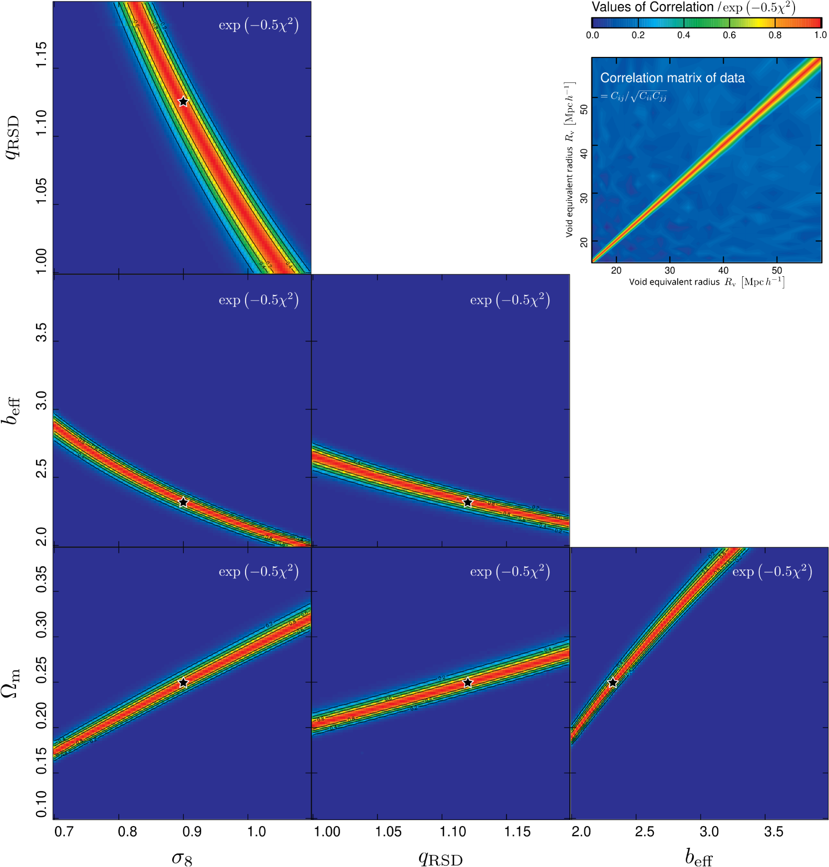
Figure 8: Different two-dimensional slices of the likelihood function of the cosmological test on the abundance of popcorn voids (top left and both bottom panels). The parameter space is composed of the matter density parameter ($\Omega_{\mathrm{m}}$), the RMS linear perturbation variance at $8~{}h^{-1}{\rm Mpc}$ ($\sigma_{8}$), the effective bias of the tracers ($b_{\mathrm{eff}}$, used in the excursion-set model) and the redshift-space expansion factor of void sizes, $q_{\rm RSD}$. Void abundances were measured assuming a fiducial cosmology with a lower value of $\Omega_{\mathrm{m}}=0.2$ and a halo sample with $M_{\mathrm{halo}}\geq 2\times 10^{12}~{}h^{-1}{\rm M_{\odot}}$ in the redshift space at $z=0.51$ (see text). The top right panel shows the correlation matrix of void abundance measurements at different equivalent void radii. Both quantities, correlation and likelihood vary between 0 and 1, and are indicated following the colour table from blue to red as shown in the colour bar in the figure. The black star indicates the expected target parameter set for this test.

5 Summary and Conclusions

In the first part of this work, Section 3, we have presented a new definition of cosmic voids and the accompanying software package where it is implemented. The code is publicly available and ready to be used in the context of cosmological simulations, we leave the implementation for use in galaxy redshift surveys for future work. The popcorn void finder defines voids as regions of maximum free-form volume with a given integrated density contrast. Due to these two features, this definition of a void can be naturally related to predictions of void abundance based on excursion-set theory. The maximum size of a void defines a unique scale associated with the adopted density contrast threshold, $\Delta_{\mathrm{v}}$. Once a prescription has been applied to associate nonlinear densities with linear values (see, for instance, the approach presented by Bernardeau, 1994), the quantity $\Delta_{\mathrm{v}}$ can be mapped onto a linear barrier that can be used to compute the crossing statistics on a linear Gaussian density field within the excursion-set theory. Although spherical void finders also provide a characteristic scale for a given $\Delta_{\mathrm{v}}$, the assumption of a spherical shape results in what we call a fragmentation problem in void identification. A single void region, depending on its size and shape, is often identified as multiple objects. This results in an artificial increase in the abundance of small voids, while the opposite occurs for larger regions. The popcorn void finder algorithm seems to solve this problem. The finder only depends on two parameters, the integrated density contrast threshold $\Delta_{\mathrm{v}}$, and the minimum radius of a popcorn sphere member, $R_{\mathrm{shot}}$, however, this last parameter can be fixed. We have shown that this radius is closely related to the shot noise scale, which is the size at which an underdense sphere is statistically significant in a given tracer sample.

After describing the void finder, we report the first significant finding of this work: the abundance of popcorn voids identified in the matter density field can be accurately described using the model proposed by Jennings et al. (2013), once a suitable linear density threshold is chosen. However, the Sheth & van de Weygaert (2004) model does not provide a viable fit. In contrast, neither of these models provides a good fit for spherical voids. The agreement between the results obtained from the popcorn void finder in simulations and the theoretical models critically depends on the choice of a linear barrier that is generally larger than expected in the spherical expansion model. This suggests the need to re-evaluate the relation between linear and nonlinear density contrast in the context of a new, perhaps non-spherical or non-isolated model. On the other hand, the accurate estimation of the shot noise radius is crucial for obtaining reliable results with the popcorn void finder. The abundance of voids in the matter field could have practical relevance if extended to the analysis of void abundances in lensing fields (see, for instance, Davies et al., 2021)

We have also analysed the shape of the popcorn voids in the matter field. We have found that they can be well described as triaxial ellipsoids, their surface area to volume ratio suggesting that their topology is not much more complex than that of ellipsoids. On the other hand, the distribution of popcorn voids in the axis-ratio space of ellipsoidal shapes is qualitatively similar to that of dark matter haloes. Voids as rare underdense regions that have triaxial shapes with predominance of prolate configurations, similar to what is expected from rare peaks in the matter field. Furthermore, this appears to be in qualitative agreement with the peak patch picture developed by Bond & Myers (1996). These authors show that in the context of the constrained statistics of extremes in a Gaussian field, the matter around the local extremes tends to be distributed in prolate configurations. In our opinion, these results originally interpreted in the context of dark matter haloes can also be applied to void shapes. In a future work we will delve into the analysis of void shapes and their possible use as cosmological probes The ellipticity of voids, in real space, have been proposed as probes of dark energy (Park & Lee, 2007; Lee & Park, 2009; Biswas et al., 2010; de Lavallaz & Fairbairn, 2011; Bos et al., 2012; Pisani et al., 2015b; Rezaei, 2020) as it can affect the shape of voids and therefore their ellipticity distribution. On the other hand, in Correa et al. (2022), we showed how the intrinsic ellipsoidal nature of voids can be detected from RSD analyses of the VGCF, and the impact of this effect on cosmological tests.

In the second part of this work, Section 4, we have presented an analysis of the abundance of popcorn voids in biased tracer samples, i.e. using different dark matter mass cutoffs, in real and redshift space. We have shown that the void abundances in dark matter halo samples are susceptible to geometric distortions due to the assumption of a given fiducial cosmology. We have also shown that the framework developed by Correa et al. (2021) can be applied in the context of popcorn voids. Using the factor $q_{\rm AP}$ derived in that work, we have established that the abundance of popcorn voids can be used to perform an Alcock-Paczyński test.

On the other hand, we also analysed the abundance of identified popcorn voids in the redshift space. Using the Correa et al. (2021) formalism, we have shown that popcorn void sizes behave qualitatively as expected, void regions are apparently larger in redshift space. We have also shown that the abundance in redshift space can also be corrected using a $q_{\rm RSD}$ factor, as derived in Correa et al. (2021). However, in the case of popcorn voids, the distortion of sizes in redshift space tends to be higher compared to what was found for spherical voids in that earlier work. This could be an indication of differences between the linear spherical expansion model and the velocity field in neighbouring regions of the popcorn voids. In a future article we will present a detailed analysis of the density and velocity field in the popcorn surroundings.

Finally, using the abundance of popcorn voids in the biased tracer field in redshift space, we have developed a cosmological proof using excursion-set theory and the Correa et al. (2021) framework. As an example of the possible exploitation of void abundances in cosmological tests, we have analysed the fit of the model in the parameter space formed by the matter density parameter $\Omega_{\mathrm{m}}$, the RMS variance of linear fluctuations $\sigma_{8}$, both as parameters of interest, and two nuisance parameters as described below. The first nuisance parameter is an effective bias, $b_{\mathrm{eff}}$, used to relate the halo density contrast threshold, used in the popcorn void finder, to the nonlinear density contrast in the matter field, used in the excursion-set model. The second parameter is the $q_{\rm RSD}$ factor, which is used to correct sizes due to redshift-space distortions. This last quantity is used as a nuisance parameter, due to our ignorance of an accurate modelling of the velocity field around popcorn voids. However, we hope, as in the case of the linear theory, that this parameter can be related to the growth rate of the structures and, after correct modelling of the bias in the velocity field, it can be used to test different gravity models.

We have found that, in the context of biased tracer samples, the Sheth & van de Weygaert (2004) model appears to be more suitable for describing the abundance of popcorn voids. The discrepancies with the Jennings et al. (2013) model may be related to a possible improper treatment of the halo bias in the volume conservation constraint. Because the aim of this work is not to develop excursion-set models, but rather to show the potential exploitation of popcorn voids in cosmological probes, we apply halo bias prescriptions at the most naive level. As we mentioned before, the halo density contrast threshold is converted to a nonlinear matter value through the effective bias, then this value is used to derive a linear density barrier using the prescription of Bernardeau (1994).

The likelihood function on the parameter space for the proposed cosmological test on the abundance of popcorn voids shows large degeneracies. However, the test shows statistical robustness, that is, there are no biases in the target parameters: the expected parameters coincide with the best fit parameters. This situation is common in various cosmological probes, however, joint analysis has been the key in the era of precision cosmology, reducing parameter constraints and allowing different paradigms to be discarded. In a recent paper Pelliciari et al. (2022) present a cosmological test using the VSF in combination with the halo mass function. Using a similar methodology, Contarini et al. (2022c) provide forecasts for the Euclid mission of the constraining power of cosmological probes based on the void abundances. In those works the cleaning and rescaling method of Ronconi & Marulli (2017) is applied over the a void sample identified using vide (Sutter et al., 2015). Even thought the differences in methodology and in the nuisance parameters, their results suggest the great potential of cosmological test of void abundances in combination with other cosmological probes.

In our opinion, the proposed cosmological test for galaxy redshift surveys using popcorn voids, given the tight contours shown in parameter space, the unbiased recovering of the parameters, and the few nuisance parameters required, has great potential to improve cosmological parameter constraints.

Data Availability

The popcorn and spherical void finders are publicly available under a MIT licence in the GitLab repository at https://gitlab.com/dante.paz/popcorn_void_finder. The data underlying this article will be shared on reasonable request to the corresponding author.

Appendix A The spherical void finder

The SVF defines a void object as the non-overlapping sphere of maximum radius with an integrated density contrast below a desired threshold $\Delta_{\mathrm{v}}$ at a given position. Then the first step is to find the locations to place the candidate spheres, called seeds. To achieve this, we first grid the simulation volume into regular cubic bins (voxcels) of side length $\delta l$. To speed up the calculation of the integrated densities, the total number of particles within each voxcel is computed. We then select voxcels for seed placement using the following procedure. Centred on each cell, we count the total number of tracers, $N_{t}$, using only the voxcels completely contained within the intersecting volume of spheres of radius, $r_{i}$, centred on the edges of the central cell. The radii $r_{i}$ are taken in increasing sequence starting at $(1+1/\sqrt{2})\delta l$ and ending at $R_{\mathrm{max}}=(N_{\mathrm{s}}+1/\sqrt{2})\delta l$, in $N_{\mathrm{s}}$ steps of $\delta l$. Then, for each radius in this sequence, we calculate a lower estimate, $\Delta_{i}$, of the density contrast for spheres centred at any position within the cell. These estimates are given by $\Delta_{i}=N_{t}/(\tfrac{4}{3}\pi{r_{i}}^{3})$. For each voxcel we keep the largest radius $r_{\mathrm{imax}}$ that has an estimated density below $\Delta_{\mathrm{v}}$. If $r_{\mathrm{imax}}$ is greater than a given radius of interest, the cell is seeded following a uniform random distribution. The number of random points seeded depends on the desired spatial resolution for the void centres, given the cell size. For each random seed, we compute the exact density within a sphere of radius $r_{\mathrm{imax}}$ centred at the position of the seed. This is done by opening the voxcels partially inside the sphere and calculating the distances of its particles to the centre. Then the particles with distances within the radius are added to the total number of particles in the voxcels contained within the sphere. If the exact density contrast is greater than $\Delta_{\mathrm{v}}$, $r_{\mathrm{imax}}$ is redefined as the next smallest radius in the radius array ($\mathrm{imax}\rightarrow\mathrm{imax}-1$) and the density calculation is repeated. This procedure is repeated until the exact density on the scale $r_{\mathrm{imax}}$ is below $\Delta_{\mathrm{v}}$ or the seed is discarded, that is, the density condition cannot be met at any radius of the array $r_{i}$.

At the end of the seeding procedure, each seed is expected to cross the exact density threshold at a radius intermediate between $r_{\mathrm{imax}}$ and $r_{\mathrm{imax}+1}$. Next, all the particles within the spherical shell contained between these two radii are ordered according to their distance from the centre. For each particle, a density is calculated using its distance as the radius and the total number of contained particles, including itself. Then the largest sphere with an integrated density contrast below $\Delta_{\mathrm{v}}$ is associated with the seed. All overlapping spheres are then removed, following an order of increasing size, keeping the largest in each pair of overlapping spheres. At the end of the process we have a set of non-overlapping spheres covering the low-density regions of the simulation box. This is the final catalogue of void objects produced by the SVF.

References

- Achitouv (2019) Achitouv I., 2019, Phys. Rev. D, 100, 123513
- Achitouv et al. (2015) Achitouv I., Neyrinck M., Paranjape A., 2015, MNRAS, 451, 3964
- Achitouv et al. (2017) Achitouv I., Blake C., Carter P., Koda J., Beutler F., 2017, Phys. Rev. D, 95, 083502
- Alcock & Paczynski (1979) Alcock C., Paczynski B., 1979, Nature, 281, 358
- Alfaro et al. (2022) Alfaro I. G., Rodriguez F., Ruiz A. N., Luparello H. E., Lambas D. G., 2022, A&A, 665, A44
- Angulo et al. (2012) Angulo R. E., Springel V., White S. D. M., Jenkins A., Baugh C. M., Frenk C. S., 2012, MNRAS, 426, 2046
- Bernardeau (1994) Bernardeau F., 1994, ApJ, 427, 51
- Biswas et al. (2010) Biswas R., Alizadeh E., Wandelt B. D., 2010, Phys. Rev. D, 82, 023002
- Bond & Myers (1996) Bond J. R., Myers S. T., 1996, ApJS, 103, 1
- Bos et al. (2012) Bos E. G. P., van de Weygaert R., Dolag K., Pettorino V., 2012, MNRAS, 426, 440
- Brunino et al. (2007) Brunino R., Trujillo I., Pearce F. R., Thomas P. A., 2007, MNRAS, 375, 184
- Buša et al. (2005) Buša J., et al., 2005, Computer Physics Communications, 165, 59
- Buša et al. (2012) Buša J., Hayryan S., Wu M.-C., Buša J., Hu C.-K., 2012, Computer Physics Communications, 183, 2494
- Cai et al. (2016) Cai Y.-C., Taylor A., Peacock J. A., Padilla N., 2016, MNRAS, 462, 2465
- Cautun et al. (2018) Cautun M., Paillas E., Cai Y.-C., Bose S., Armijo J., Li B., Padilla N., 2018, MNRAS, 476, 3195
- Ceccarelli et al. (2016) Ceccarelli L., Ruiz A. N., Lares M., Paz D. J., Maldonado V. E., Luparello H. E., Garcia Lambas D., 2016, MNRAS, 461, 4013
- Chan et al. (2014) Chan K. C., Hamaus N., Desjacques V., 2014, Phys. Rev. D, 90, 103521
- Chan et al. (2019) Chan K. C., Hamaus N., Biagetti M., 2019, Phys. Rev. D, 99, 121304
- Chan et al. (2020) Chan K. C., Li Y., Biagetti M., Hamaus N., 2020, ApJ, 889, 89
- Chuang et al. (2017) Chuang C.-H., Kitaura F.-S., Liang Y., Font-Ribera A., Zhao C., McDonald P., Tao C., 2017, Phys. Rev. D, 95, 063528
- Colberg et al. (2005) Colberg J. M., Sheth R. K., Diaferio A., Gao L., Yoshida N., 2005, MNRAS, 360, 216
- Colberg et al. (2008) Colberg J. M., et al., 2008, MNRAS, 387, 933
- Contarini et al. (2019) Contarini S., Ronconi T., Marulli F., Moscardini L., Veropalumbo A., Baldi M., 2019, MNRAS, 488, 3526
- Contarini et al. (2022a) Contarini S., Pisani A., Hamaus N., Marulli F., Moscardini L., Baldi M., 2022a, arXiv e-prints, p. arXiv:2212.03873
- Contarini et al. (2022b) Contarini S., Pisani A., Hamaus N., Marulli F., Moscardini L., Baldi M., 2022b, arXiv e-prints, p. arXiv:2212.07438
- Contarini et al. (2022c) Contarini S., et al., 2022c, A&A, 667, A162
- Correa et al. (2019) Correa C. M., Paz D. J., Padilla N. D., Ruiz A. N., Angulo R. E., Sánchez A. G., 2019, MNRAS, 485, 5761
- Correa et al. (2021) Correa C. M., Paz D. J., Sánchez A. G., Ruiz A. N., Padilla N. D., Angulo R. E., 2021, MNRAS, 500, 911
- Correa et al. (2022) Correa C. M., Paz D. J., Padilla N. D., Sánchez A. G., Ruiz A. N., Angulo R. E., 2022, MNRAS, 509, 1871
- Davies et al. (2021) Davies C. T., Cautun M., Giblin B., Li B., Harnois-Déraps J., Cai Y.-C., 2021, MNRAS, 507, 2267
- Douglass et al. (2022) Douglass K., Veyrat D., O’Neill S., BenZvi S., Zaidouni F., Guzzetti M., 2022, The Journal of Open Source Software, 7, 4033
- Elyiv et al. (2015) Elyiv A., Marulli F., Pollina G., Baldi M., Branchini E., Cimatti A., Moscardini L., 2015, MNRAS, 448, 642
- Fang et al. (2019) Fang Y., et al., 2019, MNRAS, 490, 3573
- Frenk et al. (1988) Frenk C. S., White S. D. M., Davis M., Efstathiou G., 1988, ApJ, 327, 507
- Furlanetto & Piran (2006) Furlanetto S. R., Piran T., 2006, MNRAS, 366, 467
- González (2009) González Á., 2009, Mathematical Geosciences, 42, 49
- Gonzalez et al. (2021) Gonzalez E. J., Ragone-Figueroa C., Donzelli C. J., Makler M., García Lambas D., Granato G. L., 2021, MNRAS, 508, 1280
- Górski et al. (2005) Górski K. M., Hivon E., Banday A. J., Wandelt B. D., Hansen F. K., Reinecke M., Bartelmann M., 2005, ApJ, 622, 759
- Gu et al. (2022) Gu Q., Guo Q., Zhang T., Cautun M., Lacey C., Frenk C. S., Shao S., 2022, MNRAS, 514, 390
- Hahn et al. (2007) Hahn O., Porciani C., Carollo C. M., Dekel A., 2007, MNRAS, 375, 489
- Hamaus et al. (2015) Hamaus N., Sutter P., Lavaux G., Wandelt B. D., 2015, Journal of Cosmology and Astroparticle Physics, 2015, 036
- Hamaus et al. (2017) Hamaus N., Cousinou M.-C., Pisani A., Aubert M., Escoffier S., Weller J., 2017, J. Cosmology Astropart. Phys., 7, 014
- Hamaus et al. (2020) Hamaus N., Pisani A., Choi J.-A., Lavaux G., Wandelt B. D., Weller J., 2020, J. Cosmology Astropart. Phys., 2020, 023
- Hamaus et al. (2022) Hamaus N., et al., 2022, A&A, 658, A20
- Hawken et al. (2017) Hawken A. J., et al., 2017, A&A, 607, A54
- Hawken et al. (2020) Hawken A. J., Aubert M., Pisani A., Cousinou M.-C., Escoffier S., Nadathur S., Rossi G., Schneider D. P., 2020, J. Cosmology Astropart. Phys., 2020, 012
- Hoyle & Vogeley (2002) Hoyle F., Vogeley M. S., 2002, ApJ, 566, 641
- Jennings et al. (2013) Jennings E., Li Y., Hu W., 2013, MNRAS, 434, 2167
- Lavaux & Wandelt (2010) Lavaux G., Wandelt B. D., 2010, MNRAS, 403, 1392
- Lee & Park (2009) Lee J., Park D., 2009, ApJ, 696, L10
- Marulli et al. (2016) Marulli F., Veropalumbo A., Moresco M., 2016, Astronomy and Computing, 14, 35
- Nadathur & Percival (2019) Nadathur S., Percival W. J., 2019, MNRAS, 483, 3472
- Nadathur et al. (2022) Nadathur S., et al., 2022, MNRAS, 516, 2936
- Neyrinck (2008) Neyrinck M. C., 2008, MNRAS, 386, 2101
- Padilla et al. (2005) Padilla N. D., Ceccarelli L., Lambas D. G., 2005, MNRAS, 363, 977
- Paillas et al. (2019) Paillas E., Cautun M., Li B., Cai Y.-C., Padilla N., Armijo J., Bose S., 2019, MNRAS, 484, 1149
- Park & Lee (2007) Park D., Lee J., 2007, Phys. Rev. Lett., 98, 081301
- Paz & Sánchez (2015) Paz D. J., Sánchez A. G., 2015, MNRAS, 454, 4326
- Paz et al. (2006) Paz D. J., Lambas D. G., Padilla N., Merchán M., 2006, MNRAS, 366, 1503
- Paz et al. (2013) Paz D., Lares M., Ceccarelli L., Padilla N., Lambas D. G., 2013, MNRAS, 436, 3480
- Peebles (1993) Peebles P. J. E., 1993, Principles of Physical Cosmology
- Pelliciari et al. (2022) Pelliciari D., Contarini S., Marulli F., Moscardini L., Giocoli C., Lesci G. F., Dolag K., 2022, arXiv e-prints, p. arXiv:2210.07248
- Pisani et al. (2015a) Pisani A., Sutter P. M., Hamaus N., Alizadeh E., Biswas R., Wandelt B. D., Hirata C. M., 2015a, Phys. Rev. D, 92, 083531
- Pisani et al. (2015b) Pisani A., Sutter P. M., Hamaus N., Alizadeh E., Biswas R., Wandelt B. D., Hirata C. M., 2015b, Phys. Rev. D, 92, 083531
- Platen et al. (2007) Platen E., van de Weygaert R., Jones B. J. T., 2007, MNRAS, 380, 551
- Pollina et al. (2016) Pollina G., Baldi M., Marulli F., Moscardini L., 2016, MNRAS, 455, 3075
- Pollina et al. (2017) Pollina G., Hamaus N., Dolag K., Weller J., Baldi M., Moscardini L., 2017, MNRAS, 469, 787
- Pollina et al. (2019) Pollina G., et al., 2019, MNRAS, 487, 2836
- Press & Schechter (1974) Press W. H., Schechter P., 1974, ApJ, 187, 425
- R Core Team (2013) R Core Team 2013, R: A Language and Environment for Statistical Computing. R Foundation for Statistical Computing, Vienna, Austria, http://www.R-project.org/
- Rezaei (2020) Rezaei Z., 2020, ApJ, 902, 102
- Ridley (1982) Ridley J., 1982, Mathematical Biosciences, 58, 129
- Ridley (1986) Ridley J., 1986, Mathematical biosciences, 79, 1
- Rodríguez-Medrano et al. (2022) Rodríguez-Medrano A. M., Paz D. J., Stasyszyn F. A., Rodríguez F., Ruiz A. N., Merchán M., 2022, arXiv e-prints, p. arXiv:2212.10594
- Ronconi & Marulli (2017) Ronconi T., Marulli F., 2017, A&A, 607, A24
- Ronconi et al. (2019) Ronconi T., Contarini S., Marulli F., Baldi M., Moscardini L., 2019, MNRAS, 488, 5075
- Ruiz et al. (2015) Ruiz A. N., Paz D. J., Lares M., Luparello H. E., Ceccarelli L., Lambas D. G., 2015, MNRAS, 448, 1471
- Sánchez et al. (2017) Sánchez A. G., et al., 2017, MNRAS, 464, 1640
- Schuster et al. (2019) Schuster N., Hamaus N., Pisani A., Carbone C., Kreisch C. D., Pollina G., Weller J., 2019, J. Cosmology Astropart. Phys., 2019, 055
- Sheth & van de Weygaert (2004) Sheth R. K., van de Weygaert R., 2004, MNRAS, 350, 517
- Sutter et al. (2015) Sutter P. M., et al., 2015, Astronomy and Computing, 9, 1
- Tinker et al. (2010) Tinker J. L., Robertson B. E., Kravtsov A. V., Klypin A., Warren M. S., Yepes G., Gottlöber S., 2010, ApJ, 724, 878
- Verza et al. (2019) Verza G., Pisani A., Carbone C., Hamaus N., Guzzo L., 2019, J. Cosmology Astropart. Phys., 2019, 040
- Verza et al. (2022a) Verza G., Carbone C., Pisani A., Renzi A., 2022a, arXiv e-prints, p. arXiv:2212.09740
- Verza et al. (2022b) Verza G., Carbone C., Renzi A., 2022b, ApJ, 940, L16
- Woodfinden et al. (2022) Woodfinden A., Nadathur S., Percival W. J., Radinovic S., Massara E., Winther H. A., 2022, MNRAS, 516, 4307
- de Lavallaz & Fairbairn (2011) de Lavallaz A., Fairbairn M., 2011, Phys. Rev. D, 84, 083005