Central Concentration of Asymmetric Features in Post-starburst Galaxies at $z\sim 0.8$

Abstract

We present morphological analyses of Post-starburst galaxies (PSBs) at $0.7<z<0.9$ in the COSMOS field. We fitted ultraviolet to mid-infrared multi-band photometry of objects with $i<24$ from COSMOS2020 catalogue with population synthesis models assuming non-parametric, piece-wise constant function of star formation history, and selected 94 those galaxies that have high specific star formation rates (SSFRs) of more than $10^{-9.5}$ yr^-1 in 321–1000 Myr before observation and an order of magnitude lower SSFRs within recent 321 Myr. We devised a new non-parametric morphological index which quantifies concentration of asymmetric features, $C_{A}$, and measured it as well as concentration $C$ and asymmetry $A$ on the Hubble Space Telescope /Advanced Camera for Surveys $I_{\rm F814W}$-band images. While relatively high $C$ and low $A$ values of PSBs are similar with those of quiescent galaxies rather than star-forming galaxies, we found that PSBs show systematically higher values of $C_{A}$ than both quiescent and star-forming galaxies; 36% of PSBs have $\log{C_{A}}>0.8$, while only 16% (2%) of quiescent (star-forming) galaxies show such high $C_{A}$ values. Those PSBs with high $C_{A}$ have relatively low overall asymmetry of $A\sim 0.1$, but show remarkable asymmetric features near the centre. The fraction of those PSBs with high $C_{A}$ increases with increasing SSFR in 321–1000 Myr before observation rather than residual on-going star formation. These results and their high surface stellar mass densities suggest that those galaxies experienced a nuclear starburst in the recent past, and processes that cause such starbursts could lead to the quenching of star formation through rapid gas consumption, supernova/AGN feedback, and so on.

1 Introduction

In general, galaxies can be divided into two populations, namely, star-forming galaxies (hereafter SFGs) and quiescent galaxies with little star formation (hereafter QGs). At $z\lesssim 1$, these two populations show different morphological properties; QGs tend to show centrally concentrated spheroidal shapes with little disturbed feature, while many SFGs have a (main) disk with spiral patterns and a spheroidal bulge (e.g., Roberts & Haynes, 1994; Bluck et al., 2019). The evolution of number or stellar mass density of these two populations over cosmic time suggests that some fraction of SFGs stop their star formation by some mechanism(s) and then evolved into QGs (e.g., Faber et al., 2007; Peng et al., 2010). Such transition from SFG to QG is considered to be one of the most important processes in galaxy evolution. While many mechanisms for the quenching of star formation with various decaying timescales have been proposed so far (e.g., Dekel & Silk, 1986; Barnes & Hernquist, 1996; Abadi, Moore, & Bower, 1999; Birnboim & Dekel, 2003; Martig et al., 2009; Fabian, 2012; Spilker et al., 2022), it is still unclear which mechanism plays a dominant role in galaxy evolution and how it depends on conditions such as galaxy properties, environment, epoch, and so on.

Investigating properties of galaxies in the transition phase is one of the powerful ways to reveal the physical mechanisms of quenching. In this context, post starburst galaxies (hereafter, PSBs) that experienced a strong starburst followed by quenching in the recent past have been considered to be an important population and studied intensively (see French, 2021, for recent review). PSBs are selected by their strong Balmer absorption lines and no or weak nebular emission lines such as H$\alpha$,[OII], and so on (e.g., Zabludoff et al., 1996; Dressler et al., 1999; Quintero et al., 2004). The strong Balmer absorption lines are caused by a significant contribution from A-type stars, which indicates high star formation activities in the recent past, while no significant emission lines suggest little on-going star formation in the galaxy. While fraction of PSBs is relatively small in the entire galaxy population ($\lesssim$1–2%, Zabludoff et al., 1996; Quintero et al., 2004; Blake et al., 2004; Tran et al., 2004; Goto, 2007; Wild et al., 2009; Yan et al., 2009; Vergani et al., 2010; Wong et al., 2012; Rowlands et al., 2018; Chen et al., 2019), PSBs are expected to abruptly stop their star formation after starburst and therefore considered to be in a rapid transition phase from SFG to QG. Several studies suggest that the fraction of PSBs increases with increasing redshift, and a significant fraction of galaxies at $z\sim 1$ could pass through the PSB phase when they evolved into quiescent galaxies (Wild et al., 2009; Whitaker et al., 2012; Wild et al., 2016; Wild et al., 2020).

Morphological properties of PSBs have also been investigated so far, because they can provide important clues to reveal physical origins of the starburst and rapid quenching of star formation. Many previous studies found that a significant fraction of PSBs at low and intermediate redshifts show asymmetric/disturbed features such as tidal tails (e.g., Zabludoff et al., 1996; Blake et al., 2004; Tran et al., 2004; Yamauchi & Goto, 2005; Yang et al., 2008; Pracy et al., 2009; Wong et al., 2012; D’Eugenio et al., 2020; Wilkinson et al., 2022). The morphological disturbances in many PSBs suggest that galaxy mergers/interactions could be closely related with the origin of the PSB phase. Theoretical studies with numerical simulations predicted that gas-rich major mergers cause morphological disturbances and gas infall to the centre of remnants, and then a strong starburst occurs in the central region (e.g., Barnes & Hernquist, 1991; Barnes & Hernquist, 1996; Bekki, Shioya, & Couch, 2001). Such nuclear starbursts could lead to rapid quenching of star formation through rapid gas consumption by the burst and/or gas loss/heating by supernova feedback, AGN outflow, tidal force, and so on (e.g., Bekki et al., 2005; Snyder et al., 2011; Davis et al., 2019; Spilker et al., 2022).

On the other hand, relatively massive PSBs with $M_{\rm star}\gtrsim 10^{10}M_{\odot}$ at $z\lesssim 1$ tend to have centrally concentrated early-type morphologies (e.g., Quintero et al., 2004; Tran et al., 2004; Yamauchi & Goto, 2005; Yang et al., 2008: Vergani et al., 2010; Pracy et al., 2009; Maltby et al., 2018). These results suggest that morphological changes from those with a star-forming disk to spheroidal shapes could rapidly proceed, if such changes are associated with the transition through the PSB phase. Several studies investigated asymmetric/disturbed features in PSBs as a function of time elapsed after starburst, and found that the disturbed features such as tidal tails weaken or disappear on a relatively short timescale of $\sim 0.3$ Gyr (e.g., Pawlik et al., 2016; Sazonova et al., 2021). The numerical simulations of gas-rich mergers also predict the similar decay of disturbed features on a timescale of $\sim$ 0.1–0.5 Gyr (Lotz et al., 2008; Lotz et al., 2010; Snyder et al., 2015; Pawlik et al., 2018; Nevin et al., 2019). While the asymmetric features over entire galaxies seem to rapidly weaken after starburst, observations of CO lines and dust far-infrared emission for PSBs at low redshifts suggest that significant molecular gas and dust are sustained even in those with relatively old ages of $\sim$ 500-600 Myr after starburst (Rowlands et al., 2015; French et al., 2018; Li, Narayanan, & Davé, 2019). The molecular gas and dust tend to be concentrated in the central region of those galaxies (e.g., Smercina et al., 2018; Smercina et al., 2022), and dusty disturbed features near the centre in optical images of PSBs have also been reported (e.g., Yamauchi & Goto, 2005; Yang et al., 2008; Pracy et al., 2009). Thus such disturbed/asymmetric features in the central region of PSBs could continue for longer time than those in outer regions such as tidal tails.

In this paper, we select PSBs that experienced a high star formation activity several hundreds Myr before observation followed by rapid quenching by performing SED fitting with multi-band ultraviolet (UV) to mid-infrared (MIR) photometric data including optical intermediate-bands data set in the COSMOS field (Scoville et al., 2007a) in order to statistically study morphological properties of PSBs with relatively old ages after starburst at $z\sim 0.8$. We investigate their morphological properties with non-parametric indices such as concentration and asymmetry on the Hubble Space Telescope /Advanced Camera for Surveys (HST/ACS) data, in particular, focusing on concentration of asymmetric features near the centre of these galaxies. Section 2 describes the data used in this study. In Section 3, we describe sample selection with the SED fitting and methods to measure the non-parametric morphological indices, including newly devised concentration of asymmetric features. In Section 4, we present the morphological indices of PSBs and compare them with those of SFGs and QGs. We discuss our results and their implications in Section 5, and summarise the results of this study in Section 6. Throughout this paper, we assume a flat universe with $\Omega_{\rm matter}=0.3$, $\Omega_{\Lambda}=0.7$, and $H_{0}=70$ km s^-1 Mpc^-1, and magnitudes are given in the AB system.

2 Data

In this study, we used a multi-wavelength catalogue of COSMOS2020 (Weaver et al., 2022) to construct a sample of $z\sim 0.8$ galaxies that experienced a starburst followed by rapid quenching several hundreds Myr before observation. Weaver et al. (2022) provided multi-band photometry from UV to MIR wavelengths, namely, $GALEX$ FUV and NUV (Zamojski et al., 2007), CFHT/MegaCam $u$ and $u^{*}$ (Sawicki et al., 2019), Subaru/HSC $grizy$ (Aihara et al., 2019), Subaru/Suprime-Cam $Bg^{{}^{\prime}}Vr^{{}^{\prime}}i^{{}^{\prime}}z^{{}^{\prime}}z^{{}^{\prime\prime}}$ (Taniguchi et al., 2007) and 12 intermediate and 2 narrow bands (Taniguchi et al., 2015), VISTA/VIRCAM $YJHK_{s}$ and $NB119$ (McCracken et al., 2012), and $Spitzer$/IRAC ch1–4 (Ashby et al., 2013; Steinhardt et al., 2014; Ashby et al., 2015: Ashby et al., 2018), for objects in the COSMOS field (Scoville et al., 2007a). Source detection was performed on an $izYJHK_{s}$-band combined image, and aperture photometry was done on PSF-matched images with SExtractor (Bertin & Arnouts, 1996). We used the photometry measured with 3 arcsec diameter apertures in the $GALEX$ NUV, MegaCam $u$ and $u^{*}$, HSC $grizy$, Suprime-Cam $BVi^{{}^{\prime}}z^{{}^{\prime\prime}}$ and 12 intermediate, VIRCAM $YJHK_{s}$, and IRAC ch1–4 bands for objects with $i<24$ from “CLASSIC” catalogue of COSMOS2020 in order to carry out SED fitting analysis and sample selection described in Section 3. We set the magnitude limit of $i<24$ to investigate their detailed morphology on HST/ACS data and ensure accuracy of photometry, in particular, that of the intermediate bands in the SED fitting. We excluded X-ray AGNs from our sample because the SED fitting described in the next section does not include AGN emission. The photometric offsets derived from the SED fitting with LePhare (Weaver et al., 2022) were applied to these fluxes. Furthermore, we similarly estimated additional small photometric offsets by performing the SED fitting described in the next section for isolated galaxies with spectroscopic redshifts from zCOSMOS (Lilly et al., 2007; Lilly et al., 2009) and LEGA-C (van der Wel et al., 2016; van der Wel et al., 2021) surveys, and applied them. We corrected these fluxes for Galactic extinction by using $E(B-V)$ value of the Milky Way at each object position from the catalogue.

For morphological analysis, we used COSMOS HST/ACS $I_{\rm F814W}$-band data version 2.0 (Koekemoer et al., 2007). The data have a pixel scale of 0.03 arcsec/pixel and a PSF FWHM of $\sim 0.1$ arcsec. The 50% completeness limit is $I\sim 26$ mag for sources with a half-light radius of 0.5 arcsec (Scoville et al., 2007b). We also used the Subaru/Suprime-Cam $i^{{}^{\prime}}$-band data in order to determine pixels of the ACS image which belong to the target galaxy. The reduced $i^{{}^{\prime}}$-band data have a pixel scale of 0.15 arcsec and a PSF FWHM of $\sim 1.0$ arcsec (Taniguchi et al., 2007).

3 Analysis

3.1 SED fitting

In order to select PSBs that experienced a high star formation activity followed by rapid quenching several hundreds Myr before observation, we fitted the multi-band photometry of objects with $i<24$ from the COSMOS2020 catalogue mentioned above with population synthesis models of GALAXEV (Bruzual & Charlot, 2003). For the purpose, we adopted non-parametric, piece-wise constant function of star formation history (SFH) where SFR varies among different time intervals but is constant in each interval, following previous studies (Tojeiro et al., 2007; Kelson et al., 2014; Leja et al., 2017; Leja et al., 2019; Chauke et al., 2018). We divided the look-back time for each galaxy into seven periods, namely, 0–40 Myr, 40–321 Myr, 321–1000 Myr, 1–2 Gyr, 2–4 Gyr, 4–8 Gyr, and 8–12 Gyr before observation, which are similar with those used in Leja et al. (2017). We constructed model SED templates of stars formed in the different periods by assuming Chabrier IMF (Chabrier, 2003) and constant SFR in each period. Figure 1 shows the model templates of stars formed in the seven periods for different metallicities. The model SEDs used in the fitting are based on a linear combination of the seven templates, and normalisation coefficients for the seven templates are free parameters. Thus SFHs are expressed as constant SFRs in the seven time intervals.

In order to search the best-fit values of the normalisation coefficients that provide the minimum $\chi^{2}$, we adopted Non-Negative Least Squares (NNLS) algorithm (Lawson & Hanson, 1974) following GASPEX by Magris et al. (2015),

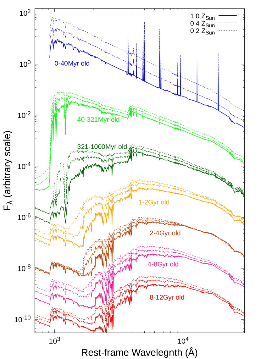
Figure 1: The model templates of stars formed in the seven periods of look-back time. They are constructed from the GALAXEV library under the assumption of constant SFR in each period. The linear combination of these templates is fitted to the observed SEDs. The short-dashed, long-dashed, and solid lines show those with 0.2, 0.4, and 1.0 $Z_{\odot}$, respectively.

while we used a simple full grid search for redshift, metallicity, and dust extinction. The NNLS algorithm basically solves a system of linear equations represented as a matrix equation, but carries out some iterations to search non-negative solutions with changing non-active (zero-value) coefficients. The templates with three stellar metallicities, namely, 0.2, 0.4, and 1.0 $Z_{\odot}$ were fitted. If we include templates with 2.5 $Z_{\odot}$, our sample of PSBs is almost the same and results in this study do not change. For simplicity, we fixed the metallicity over all the periods except for the youngest one, 0–40 Myr before observation. The metallicity of the template of 0–40 Myr was independently chosen from the same 0.2, 0.4, and 1.0 $Z_{\odot}$. We added nebular emission only in the youngest template by using PANHIT (Mawatari et al., 2016; Mawatari et al., 2020) because a contribution from the nebular emission is negligible in templates of the other older periods. In PANHIT, the nebular emission is calculated from ionising spectra of the stellar templates following Inoue (2011). We used only nebular continuum and hydrogen recombination lines from PANHIT, and recalculated fluxes of the other emission lines, namely [OII]$\lambda\lambda$3727, [OIII]$\lambda\lambda$4959,5007, [NII]$\lambda\lambda$6548,6583, [SII]$\lambda\lambda$6726, and [SIII]$\lambda\lambda$9069,9532 by using emission line ratios of local star-forming galaxies with various gas metallicities (Nagao, Maiolino, & Marconi, 2006; Vilchez & Esteban, 1996), because relatively high [OIII]/[OII] ratios in Inoue (2011) model at high metallicity lead to slight underestimates of photometric redshift for some fraction of star-forming galaxies at $z\sim$ 0.5–1.0. This is because the intermediate bands of Subaru/Suprime-Cam densely sample wavelengths around the Balmer break at these redshifts, and the deficit of the model [OII] fluxes in an intermediate band mimics the Balmer break at slightly lower redshifts. In the calculation of these emission lines, we assumed the same gas metallicity with the stellar one (i.e., 0.2, 0.4, and 1.0 $Z_{\odot}$) as in PANHIT. The fraction of ionising photons that really ionise gas rather than escape from the galaxy or are absorbed by dust is also varied from 0.1 to 1.0, while the fraction does not affect results in this study.

Linear independence among the templates is important for estimating SFHs of galaxies accurately (e.g., Magris et al., 2015). In order to select galaxies that experienced a high star formation activity followed by rapid quenching within $\sim 1$ Gyr, we chose the intervals of the periods younger than 1 Gyr so that these templates are close to be orthogonal for wavelength resolutions of the intermediate bands ($\lambda/\Delta\lambda\sim 20$). In Figure 1, one can see that variations in SED among different periods are relatively large for those with young ages of $<1$ Gyr, while differences in metallicity do not so strongly affect SEDs. In appendix, we calculated inner products between the templates with different periods/metallicities to examine the linear independence, and confirmed that ’angles’ between the templates with different periods ($<$ 1 Gyr) are relatively large, while those of the same period with different metallicities are near-parallel. Thus we expect that SFH at $<$ 1 Gyr can be reproduced relatively well, while our assumption of the fixed metallicity except for the youngest period could affect our selection for PSBs if the metallicity significantly changed between different periods. On the other hand, the variations in SED among the different periods and metallicities are much smaller for older ages of $>$ 1 Gyr, which is well known as age-metallicity degeneracy (Worthey, 1994). By setting the several periods at $>1$ Gyr, we intend to keep flexibility to avoid systematic effects of a single long period of the old age on the fitting in the younger periods, while we do not aim to accurately estimate details of SFH and metallicity at $>1$ Gyr.

For the dust extinction, we used the Calzetti law (Calzetti et al., 2000) and attenuation curves for local star-forming galaxies with different stellar masses, namely $10^{8.5}$–$10^{9.5}M_{\odot}$, $10^{9.5}$–$10^{10.5}M_{\odot}$, and $10^{10.5}$–$10^{11.5}M_{\odot}$, from Salim, Boquien, & Lee (2018). These four attenuation curves allow us to cover observed variation in 2175Å bump and reproduce correlation between the bump strength and overall slope of the attenuation curve (Salim, Boquien, & Lee, 2018). We adopted different ranges of $E(B-V)$ (or $A_{V}$) for these different attenuation curves, namely, $E(B-V)\leq 1.6$ for the Calzetti law and $E(B-V)\leq 0.4$ for those from Salim, Boquien, & Lee (2018), to take account of observed correlation between the overall slope and $V$-band attenuation, i.e., the slope tends to be steeper at smaller optical depth (Salim, Boquien, & Lee, 2018; Salim & Narayanan, 2020).

The intergalactic matter (IGM) absorption of Madau (1995) was applied to the dust-reddened model SEDs at each redshift. We took variation of the IGM absorption among lines of sight into account by adding fractional errors to fluxes in bands shorter than the rest-frame 1216 Å as in Yonekura et al. (2022).

In the fitting, we searched the minimum $\chi^{2}$ at each redshift, and calculated a redshift likelihood function, $P(z)\propto\exp(-\frac{\chi^{2}(z)}{2})$, where $\chi^{2}(z)$ is the minimum $\chi^{2}$ at each redshift. We adopted the median of the likelihood function as a redshift of each object (e.g., Ilbert et al., 2010). The photometric data with a central rest-frame wavelength longer than 25000 Å were excluded from the calculation of the minimum $\chi^{2}$ at each redshift, because our model templates do not include the dust/PAH emission. We checked accuracy of the estimated redshifts by using the spectroscopic redshift catalogues from LEGA-C and zCOSMOS. At $z_{\rm spec}<1$, 2587 and 6704 spectroscopic redshifts from LEGA-C and zCOSMOS were matched to our sample. The fraction of those with $\Delta z/(1+z_{\rm spec})>0.1$ is very small (1.35% and 0.45% for the LEGA-C and zCOSMOS samples, respectively), and the means and standard deviations of $\Delta z/(1+z_{\rm spec})$ for galaxies with $\Delta z/(1+z_{\rm spec})<0.1$ are $-0.009\pm 0.011$ and $-0.008\pm 0.012$ for the LEGA-C and zCOSMOS samples, respectively. For PSBs described in the next subsection, 27 spectroscopic redshifts from the both catalogues are available at $z_{\rm spec}<1$, and the accuracy of the estimated redshifts is almost the same as all the spec-$z$ sample with no outlier of $\Delta z/(1+z_{\rm spec})>0.1$. Such high photometric redshift accuracy is provided by the optical intermediate-bands data, which densely sample wavelengths around the Balmer/4000Å break, and is consistent with those in previous studies (Laigle et al., 2016; Weaver et al., 2022). Including the attenuation curves from Salim, Boquien, & Lee (2018) with different slopes and UV bump strengths also contributes to the accuracy of the photometric redshifts. If we use only the Calzetti attenuation law with a fixed slope and no UV bump, the fraction of catastrophic failure increases by $\sim 40$ % and the standard deviation of $\Delta z/(1+z_{\rm spec})$ increases by $\sim 30$ %.

We carried out Monte Carlo simulations to estimate probability distributions of derived physical properties such as stellar mass at the observed epoch, SFR and SSFR in the periods of look-back time. We added random shifts based on photometric errors to the observed fluxes and then performed the same SED fitting with the simulated photometries fixing the redshift to the value mentioned above. We did 1000 such simulations for each object and adopted the median values and 68% confidence intervals as the physical properties and their uncertainty, respectively.

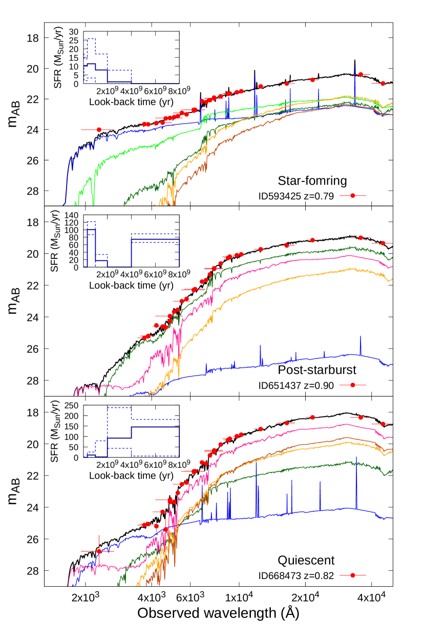
Figure 2: Examples of the SED fitting for galaxies at $z\sim 0.8$. Red circles show the observed fluxes, and vertical and horizontal error bars represent flux errors and FWHMs of the bands, respectively. The thick solid line shows the best-fit model SED, while thin lines represent contributions from stars formed in the different periods. The colours of these thin lines are the same as Figure 1. The estimated SFHs are shown in the insets, where solid and dashed lines represent the best-fit SFR and its 68% confidence interval, respectively. These three examples show different types of SFHs, namely, SFG, PSB, and QG (see text for selection criteria).

In Figure 2, we show examples of the SED fitting for galaxies at $z\sim 0.8$ classified into different types of SFHs in the next section. The contributions from stars formed in the different periods in the best-fit models and estimated SFHs are shown in the figure.

3.2 Sample selection

3.2.1 Post-Starburst Galaxies

We used the physical properties estimated from the SED fitting in the previous subsection to select galaxies that experienced active star formation followed by rapid quenching several hundreds Myr before observation. We set selection criteria with SSFRs in the three youngest periods of look-back time, namely, SSFR_0-40Myr, SSFR_40-321Myr, and SSFR_321-1000Myr. Note that we define these SSFRs as SFRs in these periods divided by stellar mass at the observed epoch (e.g., SSFR${}_{\rm 0-40Myr}=$ SFR${}_{\rm 0-40Myr}/M_{\rm star,0}$) to easily compare the SSFRs among the different periods. Thus the SSFRs used in this study do not coincide with exact values of SFR$/M_{\rm star}$ in these periods. Our selection criteria are

$$\begin{split}&{\rm SSFR}_{\rm 321-1000Myr}>10^{-9.5}\hskip 2.84526pt{\rm yr}^{-1}\hskip 2.84526pt\&\\ &{\rm SSFR}_{\rm 40-321Myr}<10^{-10.5}\hskip 2.84526pt{\rm yr}^{-1}\hskip 2.84526pt\&\\ &{\rm SSFR}_{\rm 0-40Myr}<10^{-10.5}\hskip 2.84526pt{\rm yr}^{-1}.\end{split}$$ (1)

This selection utilises a characteristic SED shape of stars formed in 321–1000 Myr before observation, namely, strong Balmer break, steep and red FUV and relatively flat NUV continuum, and relatively blue continuum at longer wavelength than the break (Figure 1). We used those galaxies at $0.7<z<0.9$ in this study, because the intermediate bands densely sample the rest-frame NUV to $B$ band for these redshifts and enable us to distinguish the characteristic SED of these stars from SEDs of stars formed in the other periods. Furthermore, the HST/ACS $I_{\rm F814W}$ band corresponds to the rest-frame $B$ band at $z\sim 0.8$. Since many morphological studies of galaxies have been done in the rest-frame $B$ band, we can easily compare our morphological results with the previous studies.

Since distributions of SSFR in the periods of 0–40 Myr, 40–321 Myr, and 321–1000 Myr for galaxies with $i<24$ at $0.7<z<0.9$ show a peak at $\sim 10^{-9.5}$ yr^-1, our selection picks up those galaxies whose SSFRs were comparable to or higher than the main sequence of SFGs in 321–1000 Myr before observation and then decreased at least by an order of magnitude in the last 321 Myr. We excluded galaxies with the reduced minimum $\chi^{2}>5$ from our analysis, because the estimated SSFRs are unreliable for those objects. We also discarded objects affected by nearby bright sources in the HST/ACS $I_{\rm F814W}$-band images, and confirmed that all remaining galaxies in our sample are not saturated in the $I_{\rm F814W}$-band images. Finally, there are 17459 galaxies with $i<24$ and reduced $\chi^{2}<5$ at $0.7<z<0.9$ in the HST/ACS $I_{\rm F814W}$-band data, and we selected 94 PSBs.

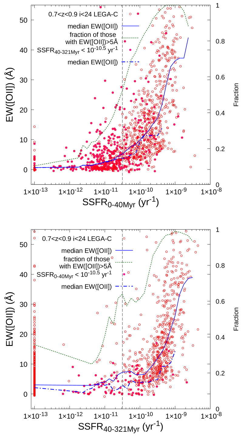
Figure 3: EW([OII]) as a function of SSFR_0-40Myr (top) and SSFR_40-321Myr (bottom) for our sample galaxies with the spectroscopic measurements by LEGA-C (van der Wel et al., 2021). Open circles show all the galaxies with $i<24$ at $0.7<z<0.9$, and solid circles represent those with SSFR${}_{\rm 40-321Myr}<10^{-10.5}$ yr^-1 in the top panel and those with SSFR${}_{\rm 0-40Myr}<10^{-10.5}$ yr^-1 in the bottom panel. Those with SSFR $<10^{-13}$ yr^-1 (SSFR $=0$ for most cases) are plotted at $10^{-13}$ yr^-1. The solid and dashed-dotted lines show the median values of EW([OII]) in SSFR bins with a width of $\pm$ 0.25 dex for all the galaxies and those with SSFR${}_{\rm 40-321Myr}<10^{-10.5}$ yr^-1 (top panel) or SSFR${}_{\rm 0-40Myr}<10^{-10.5}$ yr^-1 (bottom panel), respectively. The short-dashed line shows the fraction of those with EW([OII]) $>$ 5Å. The vertical long-dashed line shows the boundary of SSFR $=10^{-10.5}$ yr^-1, and selected PSBs have lower SSFRs than this value.

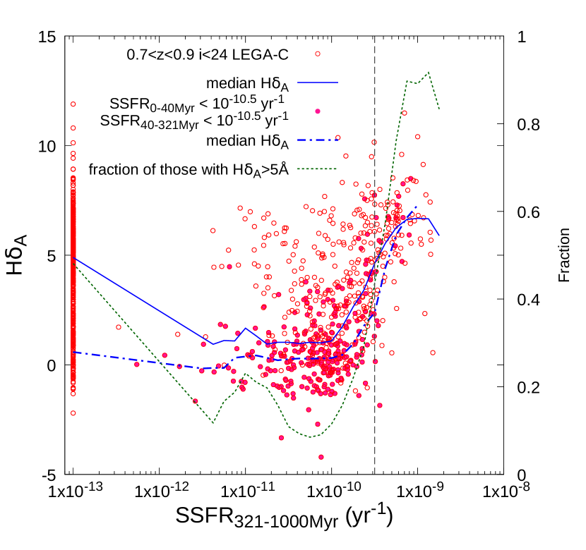
Figure 4: H$\delta_{\rm A}$ as a function of SSFR_321-1000Myr for the sample galaxies with the spectroscopic measurements by LEGA-C. Open circles show all the galaxies with $i<24$ at $0.7<z<0.9$, and solid circles represent those with SSFR${}_{\rm 0-40Myr}<10^{-10.5}$ yr^-1 and SSFR${}_{\rm 40-321Myr}<10^{-10.5}$ yr^-1. Those with SSFR${}_{\rm 321-1000Myr}<10^{-13}$ yr^-1 are plotted at $10^{-13}$ yr^-1. The solid and dashed-dotted lines show the median values of H$\delta_{\rm A}$ in SSFR_321-1000Myr bins with a width of $\pm$ 0.25 dex for all the galaxies and those with SSFR${}_{\rm 0-40Myr}<10^{-10.5}$ yr^-1 and SSFR${}_{\rm 40-321Myr}<10^{-10.5}$ yr^-1. The short-dashed line shows the fraction of those with H$\delta_{\rm A}>$ 5Å. The vertical long-dashed line shows the boundary of SSFR${}_{\rm 321-1000Myr}=10^{-9.5}$ yr^-1, and selected PSBs have higher SSFR_321-1000Myr than this value.

In order to check relation between our selection method and the spectroscopic selection for PSBs used in previous studies, we compared the estimated SSFRs in the youngest three periods with spectroscopic indices of [OII] emission and H$\delta$ absorption lines from the LEGA-C survey (van der Wel et al., 2021). For the purpose, we searched for galaxies with $i<24$ and the reduced $\chi^{2}<5$ at $0.7<z<0.9$ in the LEGA-C catalogue, and found 1265 matched objects. We used EW([OII]) and H$\delta_{\rm A}$ indices from the LEGA-C catalogue. The H$\delta_{\rm A}$ index is corrected for contribution from the emission line (van der Wel et al., 2021). The upper panel of Figure 3 shows EW([OII]) as a function of SSFR_0-40Myr. One can see that EW([OII]) tends to increase with increasing SSFR_0-40Myr, while there is a relatively large scatter at a given SSFR_0-40Myr. At SSFR${}_{\rm 0-40Myr}<10^{-10.5}$ yr^-1, the median EW([OII]) becomes $\lesssim 5$ Å, which is often used as one of the spectroscopic criteria for PSBs, and the fraction of those with EW([OII]) $>5$ Å is less than $\sim 0.5$. Solid circles in the panel show those with SSFR${}_{\rm 40-321Myr}<10^{-10.5}$ yr^-1, and therefore those solid circles at SSFR${}_{\rm 0-40Myr}<10^{-10.5}$ yr^-1 represent objects whose both SSFR_0-40Myr and SSFR_40-321Myr are lower than $10^{-10.5}$ yr^-1. Their median EW([OII]) is less than $\sim 4$ Å at SSFR${}_{\rm 0-40Myr}<10^{-10.5}$ yr^-1. The bottom panel of Figure 3 shows relation between SSFR_40-321Myr and EW([OII]). The similar trend as in the upper panel can be seen, although the median EW([OII]) at SSFR${}_{\rm 40-321Myr}\sim 10^{-10.5}$ yr^-1 is slightly higher ($\sim 7$ Å).

The median EW([OII]) for those galaxies with both SSFR${}_{\rm 0-40Myr}<10^{-10.5}$ yr^-1 and SSFR${}_{\rm 40-321Myr}<10^{-10.5}$ yr^-1 is only $\sim 1.3$ Å, and the fraction of those with EW([OII]) $>5$ Å is $\sim 0.24$. Thus the criteria of low SSFR_0-40Myr and SSFR_40-321Myr can select those galaxies with low EW([OII]), although some fraction of galaxies with EW([OII]) $>5$ Å can be included in our sample. The relatively high EW([OII]) seen in some of those galaxies could be caused by shock or weak AGN rather than star formation, as some previous studies reported that a fraction of “H$\delta$ strong” galaxies with rapidly declining SFHs show detectable [OII] emission lines (e.g., Yan et al., 2006; Pawlik et al., 2018).

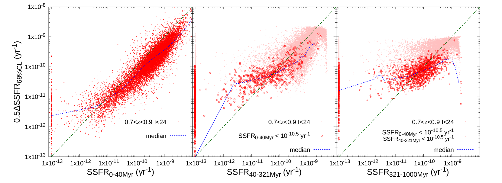
Figure 5: left: The uncertainty of SSFR_0-40Myr estimated in the SED fitting for all the sample galaxies with $i<24$ at $0.7<z<0.9$. Half widths of the 68% confidence interval of SSFR_0-40Myr are shown as a function of SSFR_0-40Myr itself. Those with SSFR${}_{\rm 0-40Myr}<10^{-13}$ yr^-1 are plotted at $10^{-13}$ yr^-1. The dashed line shows the median values in SSFR_0-40Myr bins with a width of $\pm$ 0.125 dex. middle: The same as the left panel but for SSFR_40-321Myr. While magenta dots show all the galaxies with $i<24$ at $0.7<z<0.9$, red open circles represent those with SSFR${}_{\rm 0-40Myr}<10^{-10.5}$ yr^-1. The dashed line shows the median values in SSFR_40-321Myr bins for those with SSFR${}_{\rm 0-40Myr}<10^{-10.5}$ yr^-1. right: The same as the left panel but for SSFR_321-1000Myr. Magenta dots show all the sample galaxies, and red open circles represent those with SSFR${}_{\rm 0-40Myr}<10^{-10.5}$ yr^-1 and SSFR${}_{\rm 40-321Myr}<10^{-10.5}$ yr^-1. The dashed line shows the median values in SSFR_321-1000Myr bins for those with SSFR${}_{\rm 0-40Myr}<10^{-10.5}$ yr^-1 and SSFR${}_{\rm 40-321Myr}<10^{-10.5}$ yr^-1.

Figure 4 shows H$\delta_{\rm A}$ as a function of SSFR_321-1000Myr. The H$\delta_{\rm A}$ index increases with increasing SSFR_321-1000Myr at SSFR${}_{\rm 321-1000Myr}\gtrsim 10^{-10}$ yr^-1. The median H$\delta_{\rm A}$ is $\sim 1$ Å at SSFR${}_{\rm 321-1000Myr}\sim 10^{-10}$ yr^-1 and increases to $\sim 7$Å around SSFR${}_{\rm 321-1000Myr}\sim 10^{-9}$ yr^-1. A relatively high median H$\delta_{\rm A}$ value at SSFR${}_{\rm 321-1000Myr}=10^{-13}$ yr^-1 (SSFR${}_{\rm 321-1000Myr}=0$ for most cases) is caused by those galaxies with high SSFR_0-40Myr and/or SSFR_40-321Myr. When we limit to those galaxies with SSFR${}_{\rm 0-40Myr}<10^{-10.5}$ yr^-1 and SSFR${}_{\rm 40-321Myr}<10^{-10.5}$ yr^-1 (solid circles in the figure), the median H$\delta_{\rm A}$ is $\sim 1$ Å at SSFR${}_{\rm 321-1000Myr}\lesssim 10^{-10.5}$ yr^-1, and the rapid increase at SSFR${}_{\rm 321-1000Myr}>10^{-10}$ yr^-1 remains. Those solid circles at SSFR${}_{\rm 321-1000Myr}>10^{-9,5}$ yr^-1 correspond to selected PSBs. For PSBs, the median H$\delta_{\rm A}$ is $\sim 6$Å  and 14 out of 19 those galaxies have H$\delta_{\rm A}>5$ Å, which is often used as a criterion for PSB or “H$\delta$ strong” galaxies. Therefore, we expect that many of our PSBs satisfy the spectroscopic selection used in the previous studies, namely, relatively high H$\delta_{\rm A}$ and low EW([OII]), while our selection picks up those galaxies with quenching several hundreds Myr before observation and probably misses those with more recent quenching within several tens to a hundred Myr.

In Figure 5, we show half widths of the 68% confidence intervals of SSFR_0-40Myr, SSFR_40-321Myr, and SSFR_321-1000Myr as a function of SSFR itself. In the middle panel, we separately plot the uncertainty of SSFR_40-321Myr for those galaxies with SSFR${}_{\rm 0-40Myr}<10^{-10.5}$ yr^-1 with red circles as well as all galaxies (magenta dots), because the uncertainty tends to be larger when younger population dominates in the SED and vice versa. The uncertainty of SSFR_321-1000Myr for those with SSFR${}_{\rm 0-40Myr}<10^{-10.5}$ yr^-1 and SSFR${}_{\rm 40-321Myr}<10^{-10.5}$ yr^-1 are similarly shown as red circles in the right panel. In the left panel, the median uncertainty of SSFR_0-40Myr is less than factor of 2 at SSFR${}_{\rm 0-40Myr}\gtrsim 10^{-10.5}$ yr^-1, while the fractional error is larger at lower SSFRs. The median uncertainty of SSFR_0-40Myr is less than factor of 2 at SSFR${}_{\rm 0-40Myr}\gtrsim 10^{-10.5}$ yr^-1. While the uncertainty of SSFR_40-321Myr tends to be slightly larger than that of SSFR_0-40Myr in the middle panel, galaxies with SSFR${}_{\rm 0-40Myr}<10^{-10.5}$ yr^-1 show the similar uncertainty at SSFR${}_{\rm 40-321Myr}\gtrsim 10^{-10}$ yr^-1, where the median value is less than factor of 2. The uncertainty of SSFR_321-1000Myr is larger than those of SSFR_0-40Myr and SSFR_40-321Myr (magenta dots in the right panel), which reflects the fact that SED of older stellar population is more easily overwhelmed by those of younger populations. Nevertheless, we can constrain SSFR_321-1000Myr within a factor of 2 at SSFR${}_{\rm 321-1000Myr}\gtrsim 10^{-10}$ yr^-1 for galaxies with low SSFR_0-40Myr and SSFR_40-321Myr (red circles in the panel).

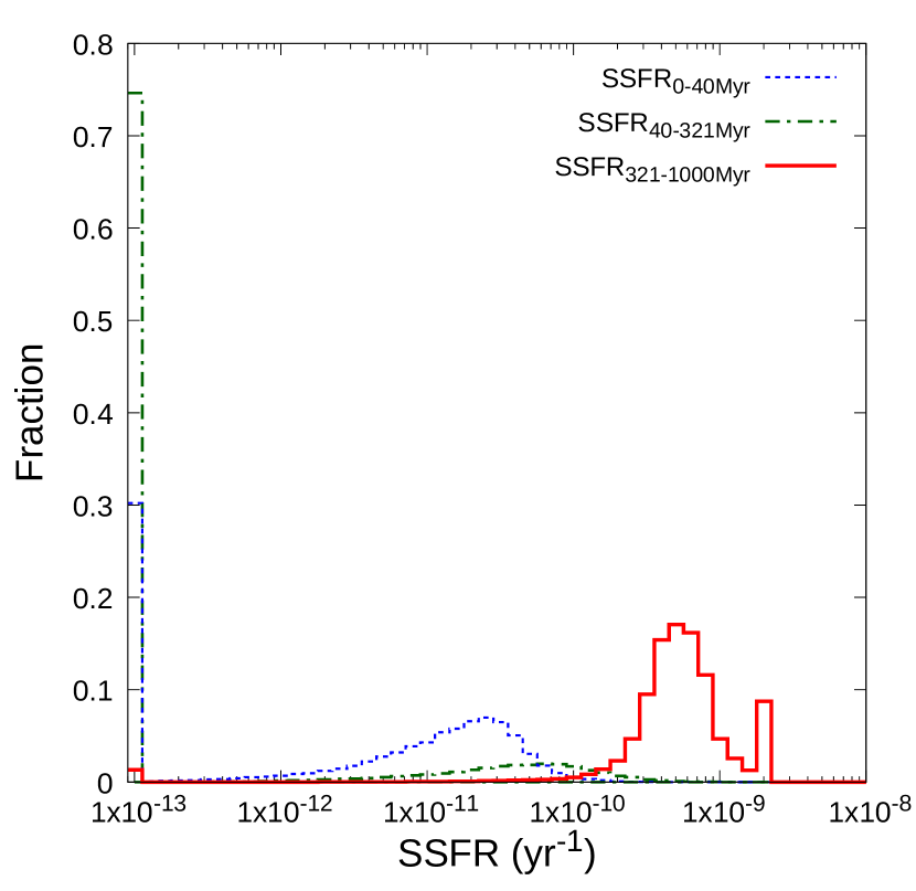
Figure 6: Average probability distributions of SSFR_0-40Myr (dashed), SSFR_40-321Myr (dashed-dotted), and SSFR_321-1000Myr (solid) estimated in the SED fitting for 94 PSBs in our sample. The distributions for each PSB are calculated from the Monte Carlo simulations (see text for details), and those averaged over the 94 PSBs are shown. The probabilities of SSFR $<10^{-13}$ yr^-1 are counted in a bin at $10^{-13}$ yr^-1.

In Figure 6, we show combined probability distributions of SSFR_0-40Myr, SSFR_40-321Myr, and SSFR_321-1000Myr for 94 PSBs to check whether these galaxies show significantly declining SFHs in the recent past even if the uncertainty is considered. We averaged these probability distributions of SSFRs calculated from the Monte Carlo simulations described in the previous subsection over those PSBs with equal weight. One can see that the probability distribution of SSFR_321-1000Myr is clearly higher than those of SSFR_0-40Myr and SSFR_40-321Myr. The probability of SSFR${}_{\rm 321-1000Myr}>$2–3$\times 10^{-10}$ yr^-1 is high, while that of SSFR${}_{\rm 40-321Myr}>10^{-10}$ yr^-1 is very low (SSFR${}_{\rm 40-321Myr}=0$ in most cases). The distribution of SSFR_0-40Myr has a peak around $2\times 10^{-11}$ yr^-1, and there is only a very small probability of SSFR${}_{\rm 0-40Myr}>10^{-10}$ yr^-1. Therefore, we expect that most of these PSBs had experienced a high star formation activity in 321–1000Myr before observation and then rapidly decreased their SFRs.

3.2.2 Star-forming & Quiescent Galaxies

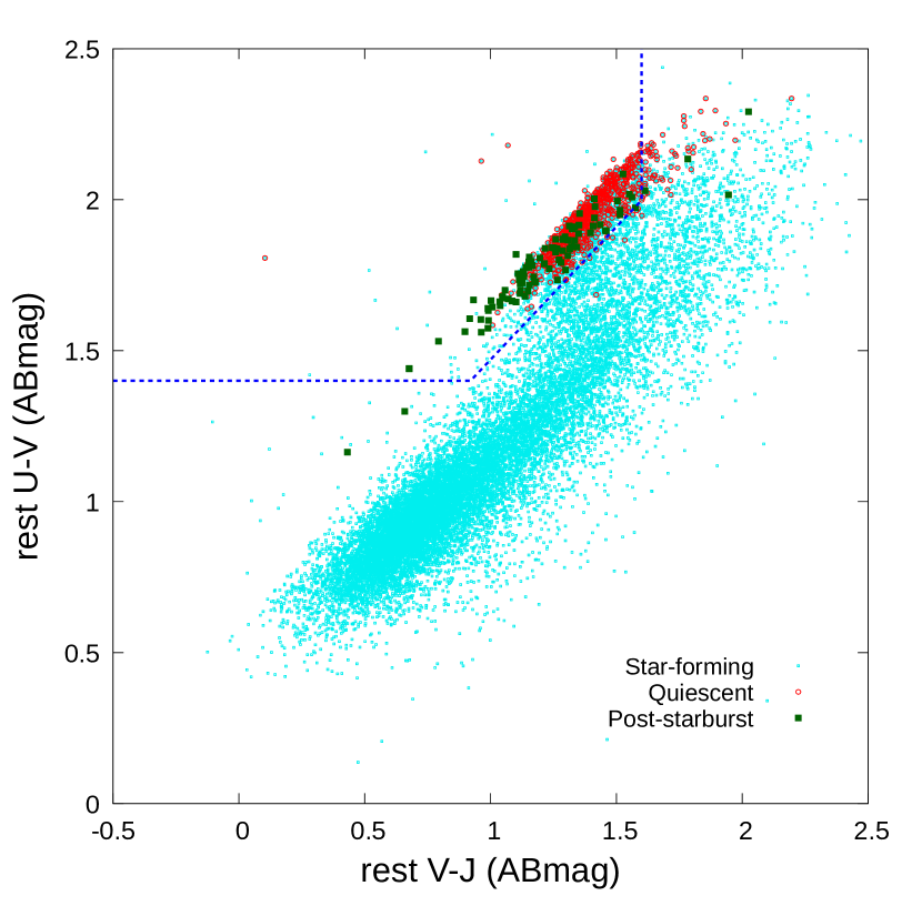
Figure 7: Rest-frame $U-V$ vs. $V-J$ two-colour diagram for SFGs (cyan dot), QGs (red open circle), and PSBs (green solid square) in our sample. The dashed line shows the colour criteria for QGs by Williams et al. (2009).

We also constructed comparison samples of normal SFGs and QGs in the same redshift range. From those galaxies with $i<24$ and the reduced minimum $\chi^{2}<5$ at $0.7<z<0.9$, we selected those objects with SSFR${}_{\rm 0-40Myr}=10^{-10}$–$10^{-9}$ yr^-1 and SSFR${}_{\rm 40-321Myr}=10^{-10}$–$10^{-9}$ yr^-1 as SFGs. Since the both distributions of SSFR_0-40Myr and SSFR_40-321Myr show a peak around $10^{-9.5}$ yr^-1, these galaxies are on and around the main sequence at least in the last $\sim 300$ Myr. We did not use SSFR_321-1000Myr in the criteria for SFGs, because the uncertainty of SSFR_321-1000Myr tends to be large for those galaxies with relatively high SSFR_0-40Myr and/or SSFR_40-321Myr (Figure 5).

For QGs, we selected galaxies with low SSFRs within recent 1 Gyr, namely, SSFR${}_{\rm 0-40Myr}<10^{-10.5}$ yr^-1 & SSFR${}_{\rm 40-321Myr}<10^{-10.5}$ yr^-1 & SSFR${}_{\rm 321-1000Myr}<10^{-10.5}$ yr^-1. We did not use those in the older periods than 1 Gyr in the criteria, because it is difficult to strongly constrain detailed SFHs older than 1 Gyr due to the degeneracy mentioned above (Figure 1). On the other hand, those QGs with a high SSFR_1-2Gyr could be similar with PSBs in that they had experienced a starburst at slightly earlier epoch than PSBs followed by rapid quenching. Thus we check results for those galaxies in Section 5.1.

Finally, we selected 6581 SFGs and 670 QGs with $i<24$ and the reduced $\chi^{2}<5$ at $0.7<z<0.9$. Examples of the SED fitting for these galaxies are shown in Figure 2. In Figure 7, we plot these SFGs, QGs, and PSBs in the rest-frame $U-V$ vs. $V-J$ two-colour plane in order to compare our classification with those in previous studies. The rest-frame colours were estimated from the best-fit model templates in the SED fitting. The dashed line in the figure shows the criteria for QGs by Williams et al. (2009). One can see that most of QGs and PSBs satisfy the criteria, while some galaxies show redder $U-V$ and $V-J$ colours due to relatively large dust extinction. PSBs tend to have bluer colours than QGs, which suggests younger stellar ages and more recent quenching of star formation. If we use the rotated system of coordinates introduced by Belli, Newman, & Ellis (2019) on the two-colour diagram, our PSBs show $S_{\rm Q}=$ 1.60–2.55, while QGs have $S_{\rm Q}=$ 2.05–2.65. The range of $S_{\rm Q}$ for our PSBs are similar with that of the spectroscopic sample at $z=$ 1.0–1.5 in Belli, Newman, & Ellis (2019). Such distribution in the two-colour plane is consistent with those in previous studies of PSBs (e.g., Wild et al., 2014; Wild et al., 2020; D’Eugenio et al., 2020; Wu et al., 2020). On the other hand, most SFGs are outside of the selection area in the plane, although a small fraction of those galaxies enter the area near the boundary. Thus our classification with the SED fitting is consistent with those in the previous studies, while our PSB selection could miss those with very recent quenching of star formation, for example, within $\sim$ 100 Myr.

3.3 Morphological analysis

3.3.1 Preparation

In this study, we used three non-parametric morphological indices, namely, concentration $C$, asymmetry $A$, and concentration of asymmetric features $C_{A}$, to investigate morphological properties of PSBs. We measured these indices on the HST/ACS $I_{\rm F814W}$-band images, while we defined pixels that belong to the object in the Subaru/Suprime-Cam $i^{{}^{\prime}}$-band data in order to keep consistency with the object detection and SED analysis carried out with the ground-based data, and to include discrete features/substructures such as knots, tidal tails, and so on in the analysis.

We cut a 12” $\times$ 12” region centred on the object coordinate of the ACS and Suprime-Cam data for each galaxy. At first, we ran SExtractor version 2.5.0 (Bertin & Arnouts, 1996) on the $i^{{}^{\prime}}$-band images by using the RMS maps (Capak et al., 2007) to scale detection threshold. The detection threshold of 0.6 times RMS values from the RMS map over 25 connected pixels was used. We aligned segmentation maps output by SExtractor to the ACS $I_{\rm F814W}$-band images with a smaller pixel scale, and used these maps to identify pixels that belong to the object in the $I_{\rm F814W}$-band images.

While we basically used pixels identified by the segmentation map from the $i^{{}^{\prime}}$-band data, we added and excluded some pixels that belong to objects/substructures detected in the $I_{\rm F814W}$-band images across the boundary defined by the segmentation map. For this adjustment, we also ran SExtractor on the $I_{\rm F814W}$-band images with a detection threshold of 1.2 times local background root mean square over 12 connected pixels. If more than half pixels of a source detected in the $I_{\rm F814W}$-band data are included in the object region defined by the $i^{{}^{\prime}}$-band segmentation map, we included all pixels of this source in the analysis and added some pixels outside of the object region if exist. On the other hand, if less than half pixels of the source is included, we masked and excluded all pixels of this source from the analysis as another object. We used the adjusted object region to measure the morphological indices for each galaxy.

We estimated pixel-to-pixel background fluctuation in the 12” $\times$ 12” region of the $I_{\rm F814W}$-band data by masking the object region and pixels that belong to the other objects with the segmentation map. We then defined pixels higher than 1$\sigma$ value of the background fluctuation in the object region as the object, and masked the other pixels less than 1$\sigma$ in the region.

3.3.2 Concentration

Following previous studies such as Kent (1985) and Bershady, Jangren, & Conselice (2000), we measured the concentration index defined as $C=r_{80}/r_{20}$, where $r_{80}$ and $r_{20}$ are radii which contain 80% and 20% of total flux of the object. The total flux was estimated as a sum of the pixels higher than 1$\sigma$ value of the background fluctuation in the object region. Since the object region is defined by an extent of the object in the $i^{{}^{\prime}}$-band data, which is often wider than that in the ACS $I_{\rm F814W}$-band data, contribution from background noise higher than the 1$\sigma$ value is non negligible. In order to estimate this contribution, we made sky images by replacing pixels in the object region with randomly selected ones that do not belong to any objects in the 12” $\times$ 12” field. All pixels outside the object region in the sky image were masked with zero value. We defined pixels higher than 2$\sigma$ in the object image as object-dominated region, and masked pixels at the same coordinates with this region in the sky image, because no biased contribution from noises is expected for those pixels with high object fluxes. We summed up pixels higher than 1$\sigma$ value in the sky image except for the object-dominated region, and subtracted this from the total flux of the object.

We then measured a growth curve with circular apertures centred at a flux-weighted mean position of the object pixels to estimate $r_{80}$ and $r_{20}$. In measurements of the growth curve, the similar subtraction of the background contribution was performed with the same sky image. We made 20 sky images for each object and repeated the measurements of $C$, and adopted their mean and standard deviation as $C$ and its uncertainty, respectively.

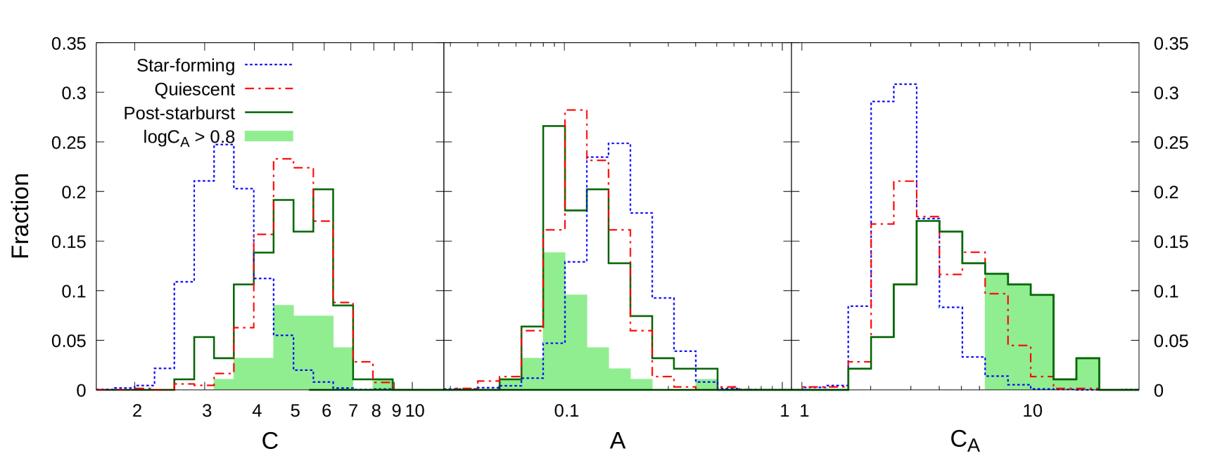
Figure 8: Distributions of the morphological indices, $C$, $A$, and $C_{A}$ for SFGs (blue dashed), QGs (red dotted-dashed), and PSBs (green solid) in our sample. The light-green solid histogram represents the contribution from those PSBs with $\log{C_{A}}>0.8$.

3.3.3 Asymmetry

We used the Asymmetry index defined by previous studies (Schade et al., 1995; Abraham et al., 1996; Conselice, Bershady, & Jangren, 2000) to measure rotation asymmetry of our sample galaxies. The asymmetry index $A$ was calculated by rotating the object image by 180 degree and subtracting it from the original image as

$$A=\frac{0.5\Sigma|I_{\rm O}-I_{180}|}{\Sigma I_{\rm O}},$$ (2)

where $I_{\rm O}$ and $I_{180}$ are pixel values in the original image and that rotated by 180 degree.

We adopted the same definition of the object pixels as in the calculation of $C$, namely, those higher than 1$\sigma$ value in the object region. The denominator of Equation (2) is the same as the total flux of the object described above, and the same correction for the background contribution was applied. In the calculation of the numerator, we chose a centre of the rotation so that a value of $A$ for the object is minimum, following Conselice, Bershady, & Jangren (2000). We searched such a centre with a step of 0.5 pixel, namely, centre of each pixel or boundary between two pixels in X and Y axes over the object region. This step size is about six times smaller than the PSF FWHM of $\sim$ 0.1 arcsec, and we can determine the rotation centre with sufficiently high accuracy to avoid significant artificial residuals in a central region due to errors of the centre. After subtracting the rotated image from the original image, we masked negative pixel values in the residual image with zero value (hereafter rotation-subtracted image). We then summed (positive) fluxes in the object region of the rotation-subtracted image.

By using the same sky image for the object as used in the calculation of total flux, we also estimated the contribution from the background noise for the rotation-subtracted image as follows. At first, we remained only pixels higher than 1$\sigma$ value in the sky image and replaced the other pixels with zero. Second, we rotated the masked sky image by 180 degree and subtracted it from that before rotation. We then summed up only positive pixels in the residual sky image except for those pixels in the object-dominated region, where pixels in the object residual image are higher than 2$\sigma$ value and the contribution from asymmetric features of the object dominates. Finally, we subtracted the estimated background contribution from the summed flux of the object residual image. By using 20 random sky images as in the estimate of $C$, we repeated the calculations described above and adopted the mean and standard deviation as $A$ and its uncertainty, respectively.

3.3.4 Concentration of Asymmetric Features

We newly devised a morphological index measuring central concentration of asymmetric features of the object, $C_{A}$. This is a combination of the asymmetry and concentration indices described above. With $C_{A}$, we aim to detect asymmetric features such as central disturbances or tidal tails, and distinguish them from those by star-forming regions in steadily star-forming disks. For example, normal star-forming disk galaxies, which usually show a central bulge with little asymmetric feature and an extended disk with star-forming regions at random positions, are expected to have relatively low concentration of the asymmetric components in their surface brightness distribution. While tidal tails tend to occur in outer regions of galaxies and lead to lower concentration, nuclear starbursts induced by gas inflow to the centre may cause disturbed features in their central region and enhance this index.

We used the same rotation-subtracted object image as in the calculation of $A$. We similarly estimated radii which contain 80% and 20% of total flux of the rotation-subtracted image, namely, $r_{A,80}$ and $r_{A,20}$, and calculated the index as $C_{A}=r_{A,80}/r_{A,20}$. To do this, we measured a growth curve on the rotation-subtracted image with circular apertures centred at the rotation centre, for which the minimum value of $A$ was obtained. The total flux of the residual image was the same as in the calculation of $A$, where the contribution from the background noise was estimated and subtracted. In measurements of $r_{A,80}$ and $r_{A,20}$, we similarly corrected for the contribution from the background noise with the same rotation-subtracted sky image. We also repeated the calculations with 20 random sky images and adopted the mean and standard deviation as $C_{A}$ and its uncertainty, respectively.

4 Results

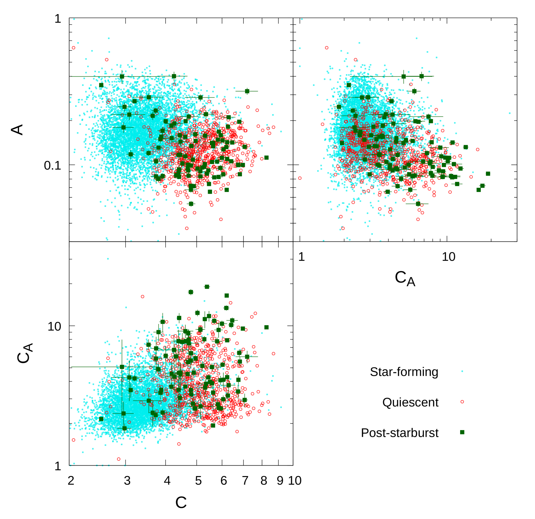
Figure 9: Scatter plots of the morphological indices, $C$, $A$, and $C_{A}$ for SFGs (cyan dot), QGs (red open circle), and PSBs (green solid square) in our sample. The error bars for PSBs show the uncertainty of the indices calculated in Section 3.3, while those for SFGs and QGs are omitted for clarity.

Figure 8 shows distributions of $C$, $A$, and $C_{A}$ for PSBs with $i<24$ at $0.7<z<0.9$ in the COSMOS field. For comparison, we also show SFGs and QGs described in Section 3.2.2. Most PSBs have $C\sim$ 3–7 and the $C$ distribution of PSBs is similar with that of QGs, while the fraction of PSBs with $C\lesssim$ 4 is slightly higher than QGs. PSBs show clearly higher $C$ values than SFGs, most of which have $C\sim$ 2.5–4.5. The $A$ distribution of PSBs shows a peak around $A\sim 0.09$ and most of PSBs have $A\sim$ 0.06–0.3. QGs show a similar range of $A$ and a peak at a slightly higher value of $A\sim$ 0.12. SFGs have a higher distribution of $A$ with a peak around $A\sim$ 0.15, and the fraction of SFGs with $A<0.1$ is small. The $C$ and $A$ indices of PSBs are similar with QGs rather than SFGs, while PSBs show slightly lower values for the both indices than QGs.

Table 1: Median values of the morphological indices for the samples with the different SFHs

sample	$C$	$A$	$C_{A}$	fraction of $\log{C_{A}}>0.8$
PSBs	$4.884\pm 0.044$	$0.1173\pm 0.0032$	$4.755\pm 0.173$	$0.362\pm 0.019$
QGs	$5.047\pm 0.016$	$0.1228\pm 0.0007$	$3.497\pm 0.042$	$0.158\pm 0.007$
SFGs	$3.396\pm 0.003$	$0.1681\pm 0.0004$	$2.723\pm 0.007$	$0.021\pm 0.001$

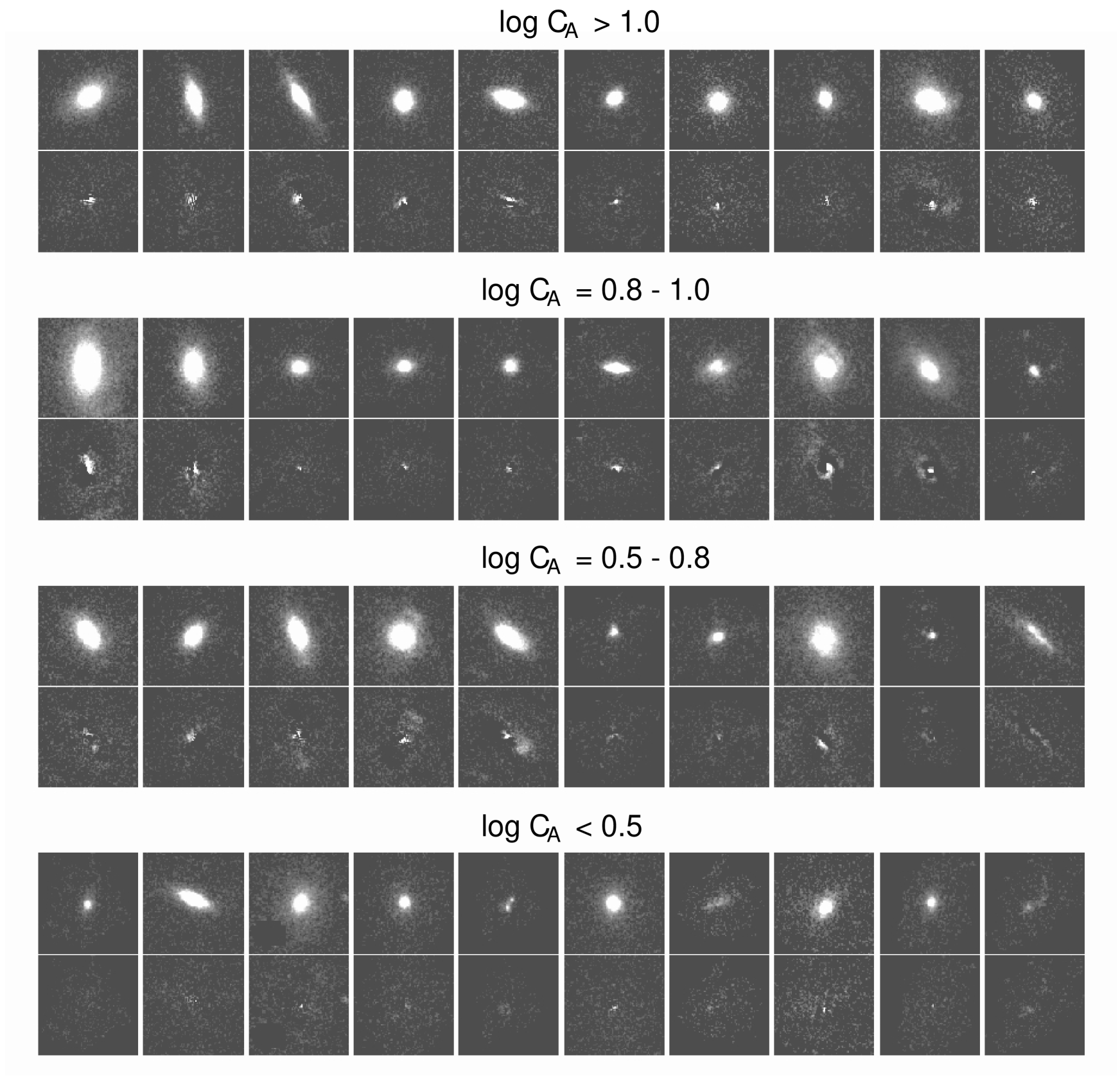
Figure 10: Examples of HST/ACS $I_{\rm F814W}$-band images for PSBs. Each panel is 3” $\times$ 3” in size. Two images are shown for each PSB: the upper panel shows the object image, and the lower panel shows the rotation-subtracted image. Four sets of the two rows of the images represent those with different $C_{A}$ values, and the $C_{A}$ values decease from top to bottom sets. In each set, galaxies are randomly selected from those with the $C_{A}$ values, and are sorted in order of increasing $A$.

In contrast with these indices, PSBs clearly tend to show higher $C_{A}$ values than QGs. While QGs show a peak around $C_{A}\sim 2.5$ and a small fraction of those with $C_{A}\gtrsim 6$, PSBs show a peak around $C_{A}\sim 4$ and more than a third of PSBs have $C_{A}\gtrsim 6$. SFGs have lower $C_{A}$ than QGs and most of them show $C_{A}<6$. We summarise median values of the morphological indices and the fraction of those with high $C_{A}$ for PSBs, QGs, and SFGs in Table 1. The errors in Table 1 are estimated with Monte Carlo simulations. In the simulations, we added random shifts based on the estimated errors (Section 3.3) to the morphological indices of each galaxy in our sample, and calculated the median values of the indices and the fraction of those with high $C_{A}$. We repeated 1000 such simulations and adopted the standard deviations of these values as the errors. The median value of $C_{A}\sim 4.8$ for PSBs is significantly higher than those of QGs and SFGs (3.5 and 2.7). The fraction of PSBs with $\log{C_{A}}>0.8$ is 36%, while those for QGs and SFGs are 16% and 2%, respectively. A significant fraction of PSBs show the high concentration of the asymmetric features. We also performed a Kolmogorov-Smirnov test to statistically examine the differences between PSBs and QGs. The probability that the $C_{A}$ distributions of PSBs and QGs are drawn from the same probability distribution is only 0.003%, while the probabilities for $C$ and $A$ are 14.6% and 15.8%, respectively.

In Figure 9, we show relationships among the morphological indices for PSBs, QGs, and SFGs. In the $C$ vs. $A$ panel, most of PSBs show relatively low $A$ and high $C$, and their distribution is similar with that of QGs. There are also a small fraction of PSBs at relatively high $A$ and low $C$, where most SFGs are located. In the $C_{A}$ vs. $A$ panel, $A$ tends to decrease with increasing $C_{A}$ for all the samples, while there is some scatter. Most of PSBs with a high value of $C_{A}\gtrsim 6$ show $A\sim$ 0.07–0.15, while there are a few PSBs with $C_{A}\gtrsim 6$ and $A>0.15$. The $A$ distribution of those with $\log{C_{A}}>0.8$ is skewed to lower values than that of all PSBs (Figure 8). Those QGs with relatively high $C_{A}$ values show similarly low values of $A$. In the $C_{A}$ vs. $C$ panel, the $C_{A}$ values of galaxies with $C<0.35$ are low, and the scatter of $C_{A}$ tends to increase with increasing $C$. PSBs with a high value of $C_{A}\gtrsim 6$ have $C\sim$ 3–8, and their distribution of $C$ is not significantly different from that of all PSBs. Even if we limit to those with a very high value of $C_{A}>10$, they have $C\sim$ 3.5–7, which is similar with those of QGs and all PSBs. Thus PSBs with high $C_{A}$ values tend to show similar $C$ and slightly lower $A$ values than all PSBs and QGs.

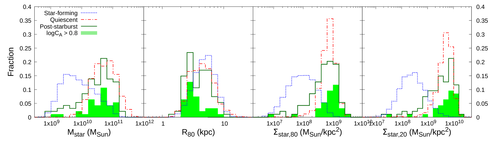
Figure 11: Distributions of stellar mass, $r_{80}$, mean surface stellar mass density within $r_{80}$ ($\Sigma_{\rm star,80}$), and that within $r_{20}$ ($\Sigma_{\rm star,20}$) for SFGs, QGs, and PSBs in our sample. The symbols are the same as Figure 8. Note that the mean surface stellar mass densities are calculated under the assumption of a constant stellar M/L ratio over the entire galaxy.

In Figure 10, we present examples of the ACS $I_{\rm F814W}$-band object images and the rotation-subtracted residual ones for PSBs with different $C_{A}$ values. Many PSBs show early-type morphologies with a significant bulge, while there are a few PSBs with low surface brightness and/or irregular morphologies. One can see that PSBs with high $C_{A}$ values show significant residuals near their centre in the rotation-subtracted images. While signal noises of the object could cause some residuals especially in the central region where their surface brightness tends to be high, the residuals show some extended structures near the centre rather than pixel-to-pixel fluctuations. These asymmetric features seem to reflect physical properties in the central region.

Those PSBs with high $C_{A}$ values tend to show relatively high surface brightness in the original images and do not show large and bright asymmetric features such as tidal tails in their outskirts. On the other hand, those with low $C_{A}$ values have more extended asymmetric features in the rotation-subtracted images. Some of them show lower surface brightness and/or irregular morphologies in the object images.

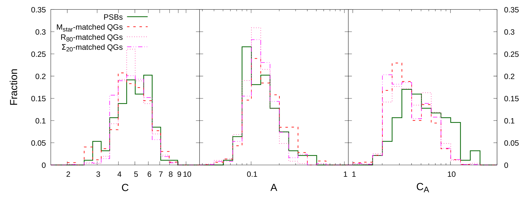
Figure 12: The same as Figure 8 but for PSBs and control samples of QGs. While the solid line shows PSBs, the dashed, dotted, and dashed-dotted lines represent $M_{\rm star}$, $r_{80}$, and $\Sigma_{20}$-matched samples of QGs, respectively.

In Figure 11, we show $M_{\rm star,0}$, $r_{80}$, and mean surface stellar mass densities within $r_{80}$ and $r_{20}$ for all PSBs and those with $\log{C_{A}}>0.8$. Note that we assumed the surface stellar mass density has the same radial profile with the $I_{\rm F814W}$-band surface brightness, and calculated the mean surface stellar mass densities as $\Sigma_{80(20)}=0.8(0.2)\times M_{\rm star,0}/(\pi r_{80(20)}^{2})$. If the galaxy has centrally concentrated young stellar population, which is often seen in PSBs as discussed in the next section, we could overestimate the surface stellar mass density in the inner region, because the contribution from the young population decreases stellar mass to luminosity ratio in the central region. While both all PSBs and those with high $C_{A}$ show similar or slightly lower stellar mass distribution with a significant tail over $10^{9}$–$10^{10}M_{\odot}$ than QGs, PSBs tend to have smaller sizes ($r_{80}$) than QGs. The fraction of relatively small galaxies with $\log{(r_{80}/{\rm kpc})}<0.5$ in all PSBs (those with $\log{C_{A}}>0.8$) is 42% (53%), which is larger than that of QGs (25%). As a result, PSBs with $\log{C_{A}}>0.8$ show higher $\Sigma_{\rm star,80}$ values than QGs, while those of the other PSBs are similar or slightly lower than QGs. The higher surface stellar mass density of those PSBs with $\log{C_{A}}>0.8$ than QGs is more clearly seen in the inner region, i.e., $\Sigma_{\rm star,20}$, although we could overestimate these values as mentioned above.

In order to examine whether morphological properties of PSBs are different from QGs or not when comparing galaxies with similar physical properties such as stellar mass, size, and surface mass density, we made control samples of QGs. By using the distributions of stellar mass in Figure 11 for PSBs and QGs, we calculated ratios of fractions, namely, $f_{\rm PSB}/f_{\rm QG}$ in each stellar mass bin. We then used the ratio in each mass bin as weight to estimate distributions of the morphological indices for a sample of QGs that effectively has the same distribution of stellar mass as PSBs. We similarly estimated distributions of the indices for $r_{80}$-matched and $\Sigma_{20}$-matched samples of QGs. Figure 12 shows comparisons of the morphological indices between PSBs and the control samples of QGs. While the $M_{\rm star}$-matched sample shows slightly higher $A$ values, the control samples basically have the similar distributions with the original sample of QGs. Even if we use the control samples of QGs, PSBs show significantly higher $C_{A}$ values than QGs, while their $C$ and $A$ values are similar with those of QGs.

5 Discussion

In this study, we fitted the photometric SEDs of galaxies with $i<24$ from COSMOS2020 catalogue with population synthesis models assuming non-parametric, piece-wise constant function of SFHs, and selected 94 PSBs with a high SSFR_321-1000Myr ($>10^{-9.5}$ yr^-1) and low SSFR_40-321Myr and SSFR_0-40Myr ($<10^{-10.5}$ yr^-1) at $0.7<z<0.9$. We measured the morphological indices, namely, $C$, $A$, and $C_{A}$ for these PSBs on the ACS $I_{\rm F814W}$-band images and compared them with SFGs whose SSFR_40-321Myr and SSFR_0-40Myr are on the main sequence ($10^{-10}$–$10^{-9}$ yr^-1) and QGs with low SSFR_321-1000Myr, SSFR_40-321Myr, and SSFR_0-40Myr values ($<10^{-10.5}$ yr^-1). We found that PSBs show systematically higher $C_{A}$ than QGs and SFGs, while their $C$ and $A$ are similar with those of QGs. The fraction of PSBs with $\log{C_{A}}>0.8$ is 36%, which is significantly higher than those of QGs and SFGs (16% and 2%). We first examine relation between $C_{A}$ and SFHs to confirm how the $C_{A}$ values are related with their physical properties, and then discuss implications of the results for evolution of these galaxies.

5.1 Relation between $C_{A}$ and SFHs

Figure 13: $C_{A}$ as a function of SSFR_0-40Myr (top), SSFR_40-321Myr (middle), and SSFR_321-1000Myr (bottom) for PSBs and those galaxies that satisfy two out of the three SSFR criteria for the PSB selection (Equation (1)). For example, those with SSFR${}_{\rm 321-1000Myr}>10^{-9.5}$ yr^-1 and SSFR${}_{\rm 40-321Myr}<10^{-10.5}$ yr^-1 are plotted in the top panel, and those objects at SSFR${}_{\rm 0-40Myr}<10^{-10.5}$ yr^-1 are PSBs. Those with SSFR $<10^{-13}$ yr^-1 are plotted at $10^{-13}$ yr^-1. The solid line shows the median values of $C_{A}$ in SSFR bins with a width of $\pm$ 0.125 dex, while the dashed line represents the fraction of those with $\log{C_{A}}>0.8$.

We found that PSBs show higher $C_{A}$ than QGs and SFGs in the previous section. We here examine relationship between $C_{A}$ and SSFRs estimated in the SED fitting. The bottom panel of Figure 13 shows $C_{A}$ distribution of those galaxies with SSFR${}_{\rm 0-40Myr}<10^{-10.5}$ yr^-1 and SSFR${}_{\rm 40-321Myr}<10^{-10.5}$ yr^-1 as a function of SSFR_321-1000Myr. Thus PSBs are located at SSFR${}_{\rm 321-1000Myr}>10^{-9.5}$ yr^-1 in this panel, while QGs are shown at SSFR${}_{\rm 321-1000Myr}<10^{-10.5}$ yr^-1. The median value of $C_{A}$ and the fraction of those with $\log{C_{A}}>0.8$ clearly increase with increasing SSFR_321-1000Myr, especially at SSFR${}_{\rm 321-1000Myr}\gtrsim 10^{-10}$ yr^-1, while scatter at a given SSFR_321-1000Myr is relatively large. This trend suggests that higher $C_{A}$ values of PSBs are related with their past star formation activities several hundreds Myr before observation. We note that those with SSFR${}_{\rm 321-1000Myr}\gtrsim 10^{-9}$ yr^-1 have slightly lower median values of $C_{A}$ and lower fraction of those with high $C_{A}$. Those galaxies with very high SSFR_321-1000Myr show relatively high asymmetry of $A\sim$ 0.15–0.40, and their asymmetric features are widely distributed over the entire galaxies, which could reduce their $C_{A}$ values. Since SSFR${}_{\rm 321-1000Myr}\sim 10^{-9}$ yr^-1 means that two thirds of the observed stellar mass had been formed in 321–1000 Myr before observation (see the next subsection for details), large morphological disturbances over the entire galaxies associated with such high star formation activities may remain at the observed epoch.

Figure 14: The same as Figure 8 but for all PSBs and those with lower SSFR_0-40Myr and SSFR_40-321Myr values. While the solid line shows all PSBs, the dashed-line (solid histogram) represents contribution from those PSBs with SSFR${}_{\rm 0-40Myr}<10^{-12}$ yr^-1 and SSFR${}_{\rm 40-321Myr}<10^{-12}$ yr^-1 (SSFR${}_{\rm 0-40Myr}<10^{-13}$ yr^-1 and SSFR${}_{40-321Myr}<10^{-13}$ yr^-1).

The top panel of Figure 13 shows the similar relationship between $C_{A}$ and SSFR_0-40Myr for those galaxies with SSFR${}_{\rm 321-1000Myr}>10^{-9.5}$ yr^-1 and SSFR${}_{\rm 40-321Myr}<10^{-10.5}$ yr^-1. The median value of $C_{A}$ and the fraction of those with $\log{C_{A}}>0.8$ decrease with increasing SSFR_0-40Myr at SSFR${}_{\rm 0-40Myr}\gtrsim 10^{-11}$ yr^-1. The relatively low values of $C_{A}$ for those galaxies with SSFR${}_{\rm 0-40Myr}=$ 10^-10–10^-9 yr^-1 on the main sequence are probably caused by star-forming regions distributed over their disk, while slightly higher $C_{A}$ values of those with SSFR${}_{\rm 0-40Myr}>10^{-9}$ yr^-1 may indicate some disturbances near the centre, for example, by nuclear starburst. The decrease of $C_{A}$ with increasing SSFR_0-40Myr at SSFR${}_{\rm 0-40Myr}\lesssim 10^{-10}$ yr^-1 suggests that the high $C_{A}$ values seen in PSBs are not closely related with residual on-going star formation. The middle panel of Figure 13 shows the SSFR_40-321Myr dependence of $C_{A}$, although most of those galaxies with SSFR${}_{\rm 321-1000Myr}>10^{-9.5}$ yr^-1 and SSFR${}_{\rm 0-40Myr}<10^{-10.5}$ yr^-1 have SSFR${}_{\rm 40-321Myr}=0$ (plotted at $10^{-13}$ yr^-1 in the figure). One can see the similar trend that those with SSFR${}_{\rm 40-321Myr}=$ 10^-10–10^-9 yr^-1 show relatively low $C_{A}$ values.

Figure 15: $C_{A}$ as a function of SSFR_1-2Gyr for QGs, which satisfy all SSFR_0-40Myr, SSFR_40-321Myr, and SSFR_321-1000Myr are less than $10^{-10.5}$ yr^-1. The solid and dashed lines are the same as Figure 13.

In Figure 14, we compare morphological indices for a sub-sample of PSBs with lower values of SSFR_0-40Myr and SSFR_40-321Myr, namely, less than 10^-12 yr^-1 and 10^-13 yr^-1 with those of all PSBs. Their distributions of the indices including $C_{A}$ are similar with those of all PSBs. This also suggests that residual star formation activities within recent $\sim 300$ Myr in our PSBs do not seem to affect their morphological properties significantly.

In Figure 15, we also examined the $C_{A}$ distribution for QGs, which have low SSFRs within the last 1 Gyr, as a function of SSFR_1-2Gyr, because 16% of these galaxies show $\log{C_{A}}>0.8$. The median value of $C_{A}$ and the fraction of QGs with $\log{C_{A}}>0.8$ increase with increasing SSFR_1-2Gyr at SSFR${}_{\rm 1-2Gyr}\gtrsim 10^{-9.5}$ yr^-1, in particular at SSFR${}_{\rm 1-2Gyr}>10^{-9.0}$ yr^-1, although the uncertainty of SSFR_1-2Gyr is relatively large as mentioned in Section 3.2. Some of those QGs with a high SSFR_1-2Gyr might have experienced a strong starburst at $\sim$ 1 Gyr before observation followed by quenching of star formation, and similarly show significant asymmetric features near the centre, which leads to high $C_{A}$ values. Since about 40% of QGs with $\log{C_{A}}>0.8$ have SSFR${}_{\rm 1-2Gyr}>10^{-9.5}$ yr^-1, some fraction of the high $C_{A}$ values seen in QGs could also be related with the past strong star formation activities.

5.2 Implications for Quenching of Star Formation in PSBs

We selected galaxies that experienced high star formation activities followed by rapid quenching several hundreds Myr before observation, by using the SED fitting with the UV to MIR photometric data including the optical intermediate-bands data. We set the selection criteria to pick up those galaxies whose SFR decreased by an order of magnitude between 321–1000 Myr and 40–321 Myr before observation (Equation (1)). Since we assumed a constant SFR in each period, the criterion of SSFR${}_{\rm 321-1000Myr}>10^{-9.5}$ yr^-1 means that $\frac{SFR_{\rm 321-1000Myr}\times(1000-321)\times 10^{6}}{M_{\rm star,0}}>0.21$, i.e., more than 20% of the observed stellar mass had been formed in the period of 321–1000 Myr before observation. Thus PSBs in this study should have a strong starburst or rather high continuous star formation activities in the period. Our selection could miss many of “H$\delta$ strong” galaxies selected by previous studies, because those galaxies whose SFRs declined on a sufficiently short timescale (e.g., less than a few hundreds Myr) could be H$\delta$ strong without such a strong starburst (e.g., Le Borgne et al., 2006; Pawlik et al., 2018). In fact, if we limit our sample to those with $M_{\rm star,0}>10^{10}M_{\odot}$, which roughly corresponds to the limiting stellar mass for our magnitude limit of $i<24$ (e.g., Satoh, Kajisawa, & Himoto, 2019), the fraction and co-moving number density of PSBs become $\sim$ 1% (76/7266) and $3.5\times 10^{-5}$ Mpc^-3, respectively. These values are smaller than those of spectroscopically selected (H$\delta$ strong) PSBs at similar redshifts in previous studies (Wild et al., 2009; Yan et al., 2009; Vergani et al., 2010; Rowlands et al., 2018), although the fraction and number density of such PSBs depend on stellar mass, environment, and selection criteria. Our PSBs seem to have the similar burst strength and time elapsed after the burst (several hundreds Myr) with those selected by photometric SEDs (Wild et al., 2016; Wild et al., 2020). While the number density of PSBs with $M_{\rm star,0}>10^{10}M_{\odot}$ in our sample is still lower than that reported in Wild et al. (2016), those of massive PSBs with $M_{\rm star}\gtrsim 10^{10.8}M_{\odot}$ are similar. The fraction of PSBs with $M_{\rm star,0}\lesssim 10^{10}M_{\odot}$ is small in our sample (the left panel of Figure 11), while Wild et al. (2016) found that the stellar mass function of those PSBs at $z=$ 0.5–1.0 shows a steep low-mass slope. Thus we could miss such relatively low-mass PSBs probably due to the magnitude limit of $i<24$.

In Figures 8 and 9, PSBs show relatively high $C$ and low $A$ values, which are similar with those of QGs. The high concentration in the surface brightness of PSBs is consistent with results by previous studies in the local universe (e.g., Quintero et al., 2004; Yamauchi & Goto, 2005; Yang et al., 2008: Pracy et al., 2009). At intermediate redshifts, several studies also found that massive PSBs with $M_{\rm star}\gtrsim 10^{10}M_{\odot}$ tend to have early-type morphology with a high concentration, while there are many low-mass PSBs with more disky morphology (Tran et al., 2004; Vergani et al., 2010: Maltby et al., 2018). On the other hand, many previous studies reported that a significant fraction of PSBs show asymmetric morphologies with tidal/disturbed features (e.g., Zabludoff et al., 1996; Blake et al., 2004; Tran et al., 2004; Yamauchi & Goto, 2005; Yang et al., 2008; Pracy et al., 2009; Wong et al., 2012; D’Eugenio et al., 2020), which seems to be inconsistent with the low $A$ values of PSBs in our sample. The discrepancy may be explained by differences in the time elapsed after starburst (hereafter, burst age). Pawlik et al. (2016) found that the fraction of local PSBs with disturbed features decreases with increasing burst age, and their $A$ and shape asymmetry $A_{S}$, which is expected to be more sensitive to faint tidal/disturbed features at outskirt, become similar with those of normal galaxies at $\sim 0.3$ Gyr after the burst. Sazonova et al. (2021) reported the similar anti-correlation between $A$ and burst age for CO-detected PSBs in the local universe. Theoretical studies with numerical simulations also suggest that such tidal/disturbed features in gas-rich major mergers weaken with time and disappear within $\sim$ 0.1–0.5 Gyr after coalescence (Lotz et al., 2008; Lotz et al., 2010; Snyder et al., 2015; Pawlik et al., 2018; Nevin et al., 2019). Since our selection method picks up those PSBs that experience a starburst several hundreds Myr before observation followed by quenching, their asymmetric features could already weaken or disappear at the observed epoch.

In this study, we found that PSBs show higher $C_{A}$ values than QGs and SFGs (Figures 8 and 9). The high $C_{A}$ values are caused by the existence of significant asymmetric features near the centre (Figure 10). Such asymmetric features near the centre of PSBs in the local universe have been reported by several studies. Yang et al. (2008) measured $A$ of 21 PSBs with strong Balmer absorption lines and weak/no [OII] emission varying aperture size, and found that the $A$ values of most PSBs increase with decreasing aperture size, which is different from those of normal spiral galaxies. Yamauchi & Goto (2005) studied colour maps of 22 PSBs with strong H$\delta$ absorption and no significant H$\alpha$ emission at $z<0.2$, and found that some of them show blue asymmetric/clumpy features near the centre in their colour maps. Pracy et al. (2009) also reported the similar irregular colour structures in the central region for two out of 10 PSBs at $z<0.2$. Sazonova et al. (2021) analysed HST/WFC3 data of 26 CO-detected PSBs at $z<0.2$ and measured their morphological parameters such as $A$, $A_{S}$, and residual flux fraction (RFF), which is the fraction of residual flux after subtracting best-fitted smooth Sérsic profile. They found that those with older burst ages tend to show relatively low $A_{S}$ and high $A$ and RFF, which suggests that internal disturbances could continue for longer time than tidal features in outer regions. For PSBs with high $C_{A}$ values in our sample, typical $r_{A,20}$ values are $\sim$ 0.08–0.13 arcsec, which corresponds to $\sim$ 0.6–1.0 kpc for galaxies at $z\sim 0.8$. Therefore, the inner asymmetric features of those galaxies are located within $\sim 1$ kpc from the centre, and the spatial resolution of $\lesssim$ 1 kpc seems to be required to reveal such high concentration of the asymmetric features.

The existence of such asymmetric features near the centre in $\sim$ 36% of our PSBs suggests that disturbances in the central region are closely related with rapid quenching of star formation. One possible scenario is that such disturbances near the centre are associated with nuclear starbursts, which occur in the galaxy mergers or accretion events and lead to the quenching through rapid gas consumption and/or gas loss/heating by supernova explosion, AGN outflow, tidal force, and so on (e.g., Bekki et al., 2005; Snyder et al., 2011; Davis et al., 2019). Several previous studies investigated radial gradients of Balmer absorption lines and colours, and found that PSBs tend to show the stronger Balmer absorption lines and bluer colours in the inner regions (Yamauchi & Goto, 2005; Yang et al., 2008; Pracy et al., 2013; Chen et al., 2019; D’Eugenio et al., 2020). These results suggest that stronger starbursts occurred in the central region of these PSBs. The numerical simulations of gas-rich galaxy mergers also predict that strong nuclear starbursts lead to the strong Balmer absorption lines and blue colours in the central region of PSBs (Bekki et al., 2005; Snyder et al., 2011; Zheng et al., 2020). In the nuclear starburst, stars are formed from kinematically disturbed infalling gas, and spatial distribution and kinematics of newly formed stars in the central region could also have disturbed/asymmetric features. Remaining dust in the central region after the burst could cause morphological disturbances in PSBs (e.g., Yang et al., 2008; Lotz et al., 2008; Sazonova et al., 2021; Smercina et al., 2022). Since the fraction of PSBs with high $C_{A}$ in our sample increases with increasing SSFR_321-1000Myr (Figure 13), their high $C_{A}$ values could be caused by such nuclear starburst several hundreds Myr before observation. Those PSBs with $\log{C_{A}}>0.8$ have the best-fit $A_{V}\lesssim$ 1.0 mag (median $A_{V}=0.5$ mag) and $[3.6]-[4.5]\sim$ 0, which are similar with or slightly lower and bluer than those of the other PSBs. While most of them are not heavily obscured by dust over the entire galaxies, some of those with high $C_{A}$ show dust-lane like features along the major axis of their surface brightness distribution in the rotation-subtracted images (Figure 10). The remaining dust in the central region could cause the asymmetric features in their morphology. Since several studies suggest that molecular gas and dust masses in PSBs at low redshifts decrease by $\sim$ 1 dex in $\sim$ 500–600 Myr after starburst (Rowlands et al., 2015; French et al., 2018; Li, Narayanan, & Davé, 2019), a significant fraction of our PSBs, which are expected to experience a starburst several hundreds Myr before observation, could have the remaining gas and dust in their central region. The relatively high $C_{A}$ values of PSBs in our sample may indicate that disturbances in the stellar and/or dust distribution near the centre tend to sustain for longer time after (nuclear) starburst than asymmetric features in outer regions such as tidal tails.

We found that PSBs, especially, those with high $C_{A}$ values tend to have smaller sizes and higher surface stellar mass densities than QGs (Figure 11). The similar smaller sizes at a given stellar mass for PSBs at low and intermediate redshifts have been reported by previous studies (Maltby et al., 2018; Wu et al., 2018; Setton et al., 2022; Chen et al., 2022). These results are consistent with the scenario where nuclear starburst causes asymmetric features near the centre in those PSBs with high $C_{A}$. The nuclear starburst is expected to increase the stellar mass density in the central region, which leads to decreases in half-light and half-mass radii of these galaxies (e.g., Wu et al., 2020). If this is the case, the half-light radii of those PSBs will gradually increase and become similar with those of QGs, because flux contribution from the young population in the central region is expected to decrease as time elapses.

Although the results in this study suggest the relationship between nuclear starburst and quenching of star formation in those PSBs, we cannot specify why their star formation rapidly declined and has been suppressed for (at least) a few hundreds Myr. Further observations of these galaxies will allow us to reveal the quenching process. NIR and FIR imaging data with similarly high spatial resolution of $\lesssim 1$ kpc scale taken with JWST and ALMA enable to investigate details of the asymmetric features near the centre in those PSBs and their origins. Physical state of molecular gas over the entire galaxies is also important to understand the quenching mechanism(s). Observing stellar absorption lines and nebular emission lines by deep optical (spatially resolved) spectroscopy allows us to study detailed stellar population and excitation state of ionised gas. Although we excluded AGNs from the sample in this study because of the difficulty of estimating non-parametric SFHs with the AGN contribution in the SED fitting, it is interesting to investigate relationship between the disturbances in the central region and AGN activity.

6 Summary

In order to investigate morphological properties of PSBs, we performed the SED fitting with the UV–MIR photometric data including the optical intermediate bands for objects with $i<24$ from COSMOS2020 catalogue, and selected 94 PSBs that experienced a high star formation activity several hundreds Myr before observation (SSFR${}_{\rm 321-1000Myr}>10^{-9.5}$ yr^-1) followed by quenching (SSFR${}_{\rm 40-321Myr}<10^{-10.5}$ yr^-1 and SSFR${}_{\rm 0-40Myr}<10^{-10.5}$ yr^-1) at $0.7<z<0.9$. We measured the morphological indices, namely, concentration $C$, asymmetry $A$, and concentration of asymmetric features $C_{A}$, on the HST/ACS $I_{\rm F814W}$-band images, and compared them with those of QGs and SFGs. Our main results are summarised as follows.

• PSBs show relatively high concentration (the median $C\sim 4.9$) and low asymmetry (the median $A\sim 0.12$), which are similar with those of QGs rather than SFGs. Our selection method, which preferentially picks up those with relatively old burst ages of several hundreds Myr, could lead to the low asymmetry.

• PSBs tend to show higher $C_{A}$ values (the median $C_{A}\sim 4.8$) than both QGs and SFGs (the median $C_{A}\sim 3.5$ and 2.7). The difference of $C_{A}$ between PSBs and QGs is significant even if we compare PSBs with $M_{\rm star}$, $r_{80}$, or $\Sigma_{20}$-matched samples of QGs. The fraction of galaxies with $\log{C_{A}}>0.8$ in PSBs is $\sim$36%, which is much higher than those of QGs and SFGs (16% and 2%). Those PSBs with high $C_{A}$ show remarkable asymmetric features near the centre, while they have relatively low overall asymmetry ($A\sim 0.1$).

• The fraction of those PSBs with $\log{C_{A}}>0.8$ increases with increasing SSFR_321-1000Myr and decreasing SSFR_0-40Myr, which indicates that the asymmetric features near the centre are closely related with the high star formation activities several hundreds Myr before observation rather than residual on-going star formation.

• Those PSBs with high $C_{A}$ tend to have higher surface stellar mass density, in particular, in the central region (e.g., $\lesssim 1$ kpc) than both QGs and the other PSBs, while most of them have the similar stellar masses of $1\times 10^{10}$–$2\times 10^{11}M_{\odot}$.

These results suggest that a significant fraction of PSBs experienced nuclear starburst in the recent past, and the quenching of star formation in these galaxies could be related with such active star formation in the central region. The high $C_{A}$ values of PSBs may indicate that the disturbances near the centre tend to sustain for longer time than those at outskirt such as tidal tails. If this is the case, $C_{A}$ could be used as morphological signs of the past nuclear starburst in those galaxies with relatively old burst ages.

Data Availability

The COSMOS2020 catalogue is publicly available at https://cosmos2020.calet.org/. The COSMOS HST/ACS $I_{\rm F814W}$-band mosaic data version 2.0 are publicly available via NASA/IPAC Infrared Science Archive at https://irsa.ipac.caltech.edu/data/COSMOS/images/acs_mosaic_2.0/. The raw data for the ACS mosaic are available via Mikulski Archive for Space Telescopes at https://archive.stsci.edu/missions-and-data/hst. The Subaru/Suprime-Cam $i{{}^{\prime}}$-band mosaic reduced data are also publicly available at https://irsa.ipac.caltech.edu/data/COSMOS/images/subaru/. The raw data for the Suprime-Cam mosaic are accessible through Subaru Telescope Archive System at https://stars.naoj.org. The zCOSMOS spectroscopic redshift catalogue is publicly available via ESO Science Archive Facility at https://www.eso.org/qi/catalog/show/65. The LEGA-C catalogue is also publicly available at https://www.eso.org/qi/catalogQuery/index/379.

Appendix A Linear independence of templates

Figure 16: The same as Figure 1, but for those convolved with a Gaussian function with FWHM of $\lambda/20\AA$, which corresponds to the wavelength resolution of the intermediate bands.

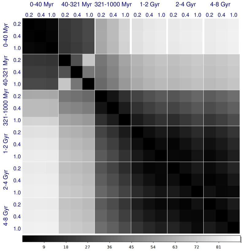
Figure 17: The angle $\theta_{ij}$ (Equation (3)) between spectral templates of stars formed in the different periods of look-back time. Results for three stellar metallicities, namely, 0.2, 0.4, and 1.0 $Z_{\odot}$ are shown for each period.

We here examine the linear independence of the model templates of stars formed in the different periods of look-back time, which were used in the SED fitting. Following Magris et al. (2015), we considered the model templates as vectors, and calculated inner (dot) products between two of these vectors for the purpose. At first, we convolved these templates with a spectral resolution of the intermediate bands, namely, $\lambda/\Delta\lambda=20$ (Figure 16), because we used the photometric SEDs in the SED fitting as described in Section 3.1. The 12 intermediate bands cover only $\sim$ 4000–8000 Å, which corresponds to the rest-frame 2000–5000 Å  at $z=$ 0.7–0.9, and the wavelength resolution becomes lower at longer wavelengths. While we here assume the resolution of $\lambda/\Delta\lambda=20$ in all wavelengths for simplicity, this does not affect results described below. We used the template of 0–40 Myr where 50% of ionising photons from stars really ionise gas and contribute to the nebular emission, but following results do not strongly depend on this fraction. We then calculate ’angle’ between the templates $T_{i}$ and $T_{j}$ as

$$\theta_{ij}=cos^{-1}\biggl{(}\frac{\sum\limits_{m}T_{i}(\lambda_{m})T_{j}(\lambda_{m})}{\sqrt{\sum\limits_{m}T_{i}(\lambda_{m})^{2}}\sqrt{\sum\limits_{m}T_{j}(\lambda_{m})^{2}}}\biggl{)},$$ (3)

where $\lambda_{m}$ is wavelength of each resolution element.

Figure 17 shows the angles between templates with different periods and metallicities. The angles between young ($<$ 321 Myr) templates and older ($>$ 1 Gyr) ones are $\sim 90^{\circ}$, while those among the older templates are nearly zero. The templates of 321–1000 Myr show intermediate angles with those of the other periods, depending on metallicity. In particular, the angle between a template of 321–1000 Myr with high metallicity and 1–2 Gyr one with low metallicity is relatively low. While this could cause some degeneracy, we expect that this does not strongly affect our results because we assume the fixed metallicity except for the youngest period. Those of the same periods with different metallicities show small angles except for 40–321 Myr ones, and effects of the different metallicities seem to be not so large. Thus we can basically differentiates contributions from the young, intermediate (321–1000 Myr), old stellar populations, while the degeneracy could affect our selection for PSBs if the metallicity of stars formed in starburst is significantly higher than older stellar populations.

References

- Abadi, Moore, & Bower (1999) Abadi M. G., Moore B., Bower R. G., 1999, MNRAS, 308, 947
- Abraham et al. (1996) Abraham R. G., van den Bergh S., Glazebrook K., Ellis R. S., Santiago B. X., Surma P., Griffiths R. E., 1996, ApJS, 107, 1
- Aihara et al. (2019) Aihara H., AlSayyad Y., Ando M., Armstrong R., Bosch J., Egami E., Furusawa H., et al., 2019, PASJ, 71, 114
- Ashby et al. (2018) Ashby M. L. N., Caputi K. I., Cowley W., Deshmukh S., Dunlop J. S., Milvang-Jensen B., Fynbo J. P. U., et al., 2018, ApJS, 237, 39
- Ashby et al. (2013) Ashby M. L. N., Willner S. P., Fazio G. G., Huang J.-S., Arendt R., Barmby P., Barro G., et al., 2013, ApJ, 769, 80
- Ashby et al. (2015) Ashby M. L. N., Willner S. P., Fazio G. G., Dunlop J. S., Egami E., Faber S. M., Ferguson H. C., et al., 2015, ApJS, 218, 33
- Barnes & Hernquist (1991) Barnes J. E., Hernquist L. E., 1991, ApJL, 370, L65
- Barnes & Hernquist (1996) Barnes J. E., Hernquist L., 1996, ApJ, 471, 115
- Bekki et al. (2005) Bekki K., Couch W. J., Shioya Y., Vazdekis A., 2005, MNRAS, 359, 949
- Bekki, Shioya, & Couch (2001) Bekki K., Shioya Y., Couch W. J., 2001, ApJL, 547, L17. doi:10.1086/31888
- Belli, Newman, & Ellis (2019) Belli S., Newman A. B., Ellis R. S., 2019, ApJ, 874, 17. doi:10.3847/1538-4357/ab07af
- Bershady, Jangren, & Conselice (2000) Bershady M. A., Jangren A., Conselice C. J., 2000, AJ, 119, 2645
- Bertin & Arnouts (1996) Bertin E., Arnouts S., 1996, A&AS, 117, 393
- Birnboim & Dekel (2003) Birnboim Y., Dekel A., 2003, MNRAS, 345, 349
- Blake et al. (2004) Blake C., Pracy M. B., Couch W. J., Bekki K., Lewis I., Glazebrook K., Baldry I. K., et al., 2004, MNRAS, 355, 713
- Bluck et al. (2019) Bluck A. F. L., Bottrell C., Teimoorinia H., Henriques B. M. B., Mendel J. T., Ellison S. L., Thanjavur K., et al., 2019, MNRAS, 485, 666
- Bruzual & Charlot (2003) Bruzual G., Charlot S., 2003, MNRAS, 344, 1000
- Calzetti et al. (2000) Calzetti D., Armus L., Bohlin R. C., Kinney A. L., Koornneef J., Storchi-Bergmann T., 2000, ApJ, 533, 682
- Capak et al. (2007) Capak P., Aussel H., Ajiki M., McCracken H. J., Mobasher B., Scoville N., Shopbell P., et al., 2007, ApJS, 172, 99
- Chauke et al. (2018) Chauke P., van der Wel A., Pacifici C., Bezanson R., Wu P.-F., Gallazzi A., Noeske K., et al., 2018, ApJ, 861, 13
- Chabrier (2003) Chabrier G., 2003, PASP, 115, 763
- Chen et al. (2022) Chen X., Lin Z., Kong X., Liang Z., Chen G., Zhang H.-X., 2022, ApJ, 933, 228
- Chen et al. (2019) Chen Y.-M., Shi Y., Wild V., Tremonti C., Rowlands K., Bizyaev D., Yan R., et al., 2019, MNRAS, 489, 5709
- Conselice, Bershady, & Jangren (2000) Conselice C. J., Bershady M. A., Jangren A., 2000, ApJ, 529, 886
- Davis et al. (2019) Davis T. A., van de Voort F., Rowlands K., McAlpine S., Wild V., Crain R. A., 2019, MNRAS, 484, 2447
- Dekel & Silk (1986) Dekel A., Silk J., 1986, ApJ, 303, 39
- D’Eugenio et al. (2020) D’Eugenio F., van der Wel A., Wu P.-F., Barone T. M., van Houdt J., Bezanson R., Straatman C. M. S., et al., 2020, MNRAS, 497, 389
- Dressler et al. (1999) Dressler A., Smail I., Poggianti B. M., Butcher H., Couch W. J., Ellis R. S., Oemler A., 1999, ApJS, 122, 51
- Faber et al. (2007) Faber S. M., Willmer C. N. A., Wolf C., Koo D. C., Weiner B. J., Newman J. A., Im M., et al., 2007, ApJ, 665, 265
- Fabian (2012) Fabian A. C., 2012, ARA&A, 50, 455
- French (2021) French K. D., 2021, PASP, 133, 072001
- French et al. (2018) French K. D., Yang Y., Zabludoff A. I., Tremonti C. A., 2018, ApJ, 862, 2
- Goto (2007) Goto T., 2007, MNRAS, 381, 187
- Ilbert et al. (2010) Ilbert O., Salvato M., Le Floc’h E., Aussel H., Capak P., McCracken H. J., Mobasher B., et al., 2010, ApJ, 709, 644
- Inoue (2011) Inoue A. K., 2011, MNRAS, 415, 2920
- Kelson et al. (2014) Kelson D. D., Williams R. J., Dressler A., McCarthy P. J., Shectman S. A., Mulchaey J. S., Villanueva E. V., et al., 2014, ApJ, 783, 110
- Kent (1985) Kent S. M., 1985, ApJS, 59, 115
- Koekemoer et al. (2007) Koekemoer A. M., Aussel H., Calzetti D., Capak P., Giavalisco M., Kneib J.-P., Leauthaud A., et al., 2007, ApJS, 172, 196
- Laigle et al. (2016) Laigle C., McCracken H. J., Ilbert O., Hsieh B. C., Davidzon I., Capak P., Hasinger G., et al., 2016, ApJS, 224, 24
- Lawson & Hanson (1974) Lawson C. L., Hanson R. J., 1974, slsp.book
- Le Borgne et al. (2006) Le Borgne D., Abraham R., Daniel K., McCarthy P. J., Glazebrook K., Savaglio S., Crampton D., et al., 2006, ApJ, 642, 48
- Leja et al. (2019) Leja J., Carnall A. C., Johnson B. D., Conroy C., Speagle J. S., 2019, ApJ, 876, 3
- Leja et al. (2017) Leja J., Johnson B. D., Conroy C., van Dokkum P. G., Byler N., 2017, ApJ, 837, 170
- Li, Narayanan, & Davé (2019) Li Q., Narayanan D., Davé R., 2019, MNRAS, 490, 1425
- Lilly et al. (2009) Lilly S. J., Le Brun V., Maier C., Mainieri V., Mignoli M., Scodeggio M., Zamorani G., et al., 2009, ApJS, 184, 218
- Lilly et al. (2007) Lilly S. J., Le Fèvre O., Renzini A., Zamorani G., Scodeggio M., Contini T., Carollo C. M., et al., 2007, ApJS, 172, 70
- Lotz et al. (2008) Lotz J. M., Jonsson P., Cox T. J., Primack J. R., 2008, MNRAS, 391, 1137
- Lotz et al. (2010) Lotz J. M., Jonsson P., Cox T. J., Primack J. R., 2010, MNRAS, 404, 590
- Madau (1995) Madau P., 1995, ApJ, 441, 18
- Magris et al. (2015) Magris C. G., Mateu P. J., Mateu C., Bruzual A. G., Cabrera-Ziri I., Mejía-Narváez A., 2015, PASP, 127, 16
- Maltby et al. (2018) Maltby D. T., Almaini O., Wild V., Hatch N. A., Hartley W. G., Simpson C., Rowlands K., et al., 2018, MNRAS, 480, 381
- Martig et al. (2009) Martig M., Bournaud F., Teyssier R., Dekel A., 2009, ApJ, 707, 250
- Mawatari et al. (2020) Mawatari K., Inoue A. K., Yamanaka S., Hashimoto T., Tamura Y., 2020, IAUS, 341, 285
- Mawatari et al. (2016) Mawatari K., Yamada T., Fazio G. G., Huang J.-S., Ashby M. L. N., 2016, PASJ, 68, 46
- McCracken et al. (2012) McCracken H. J., Milvang-Jensen B., Dunlop J., Franx M., Fynbo J. P. U., Le Fèvre O., Holt J., et al., 2012, A&A, 544, A156
- Nagao, Maiolino, & Marconi (2006) Nagao T., Maiolino R., Marconi A., 2006, A&A, 459, 85
- Nevin et al. (2019) Nevin R., Blecha L., Comerford J., Greene J., 2019, ApJ, 872, 76
- Pawlik et al. (2018) Pawlik M. M., Taj Aldeen L., Wild V., Mendez-Abreu J., Lahén N., Johansson P. H., Jimenez N., et al., 2018, MNRAS, 477, 1708
- Pawlik et al. (2016) Pawlik M. M., Wild V., Walcher C. J., Johansson P. H., Villforth C., Rowlands K., Mendez-Abreu J., et al., 2016, MNRAS, 456, 3032
- Peng et al. (2010) Peng Y.-. jie ., Lilly S. J., Kovač K., Bolzonella M., Pozzetti L., Renzini A., Zamorani G., et al., 2010, ApJ, 721, 193
- Pracy et al. (2013) Pracy M. B., Croom S., Sadler E., Couch W. J., Kuntschner H., Bekki K., Owers M. S., et al., 2013, MNRAS, 432, 3131
- Pracy et al. (2009) Pracy M. B., Kuntschner H., Couch W. J., Blake C., Bekki K., Briggs F., 2009, MNRAS, 396, 1349
- Quintero et al. (2004) Quintero A. D., Hogg D. W., Blanton M. R., Schlegel D. J., Eisenstein D. J., Gunn J. E., Brinkmann J., et al., 2004, ApJ, 602, 190
- Roberts & Haynes (1994) Roberts M. S., Haynes M. P., 1994, ARA&A, 32, 115
- Rowlands et al. (2018) Rowlands K., Wild V., Bourne N., Bremer M., Brough S., Driver S. P., Hopkins A. M., et al., 2018, MNRAS, 473, 1168
- Rowlands et al. (2015) Rowlands K., Wild V., Nesvadba N., Sibthorpe B., Mortier A., Lehnert M., da Cunha E., 2015, MNRAS, 448, 258
- Salim, Boquien, & Lee (2018) Salim S., Boquien M., Lee J. C., 2018, ApJ, 859, 11
- Salim & Narayanan (2020) Salim S., Narayanan D., 2020, ARA&A, 58, 529
- Satoh, Kajisawa, & Himoto (2019) Satoh Y. K., Kajisawa M., Himoto K. G., 2019, ApJ, 885, 81
- Sawicki et al. (2019) Sawicki M., Arnouts S., Huang J., Coupon J., Golob A., Gwyn S., Foucaud S., et al., 2019, MNRAS, 489, 5202
- Sazonova et al. (2021) Sazonova E., Alatalo K., Rowlands K., Deustua S. E., French K. D., Heckman T., Lanz L., et al., 2021, ApJ, 919, 134
- Schade et al. (1995) Schade D., Lilly S. J., Crampton D., Hammer F., Le Fevre O., Tresse L., 1995, ApJL, 451, L1
- Scoville et al. (2007a) Scoville N., Aussel H., Brusa M., Capak P., Carollo C. M., Elvis M., Giavalisco M., et al., 2007, ApJS, 172, 1
- Scoville et al. (2007b) Scoville N., Abraham R. G., Aussel H., Barnes J. E., Benson A., Blain A. W., Calzetti D., et al., 2007, ApJS, 172, 38. doi:10.1086/516580
- Setton et al. (2022) Setton D. J., Verrico M., Bezanson R., Greene J. E., Suess K. A., Goulding A. D., Spilker J. S., et al., 2022, ApJ, 931, 51
- Smercina et al. (2018) Smercina A., Smith J. D. T., Dale D. A., French K. D., Croxall K. V., Zhukovska S., Togi A., et al., 2018, ApJ, 855, 51
- Smercina et al. (2022) Smercina A., Smith J.-D. T., French K. D., Bell E. F., Dale D. A., Medling A. M., Nyland K., et al., 2022, ApJ, 929, 154
- Snyder et al. (2011) Snyder G. F., Cox T. J., Hayward C. C., Hernquist L., Jonsson P., 2011, ApJ, 741, 77
- Snyder et al. (2015) Snyder G. F., Lotz J., Moody C., Peth M., Freeman P., Ceverino D., Primack J., et al., 2015, MNRAS, 451, 4290
- Spilker et al. (2022) Spilker J. S., Suess K. A., Setton D. J., Bezanson R., Feldmann R., Greene J. E., Kriek M., et al., 2022, arXiv, arXiv:2208.13917
- Steinhardt et al. (2014) Steinhardt C. L., Speagle J. S., Capak P., Silverman J. D., Carollo M., Dunlop J., Hashimoto Y., et al., 2014, ApJL, 791, L25
- Taniguchi et al. (2007) Taniguchi Y., Scoville N., Murayama T., Sanders D. B., Mobasher B., Aussel H., Capak P., et al., 2007, ApJS, 172, 9
- Taniguchi et al. (2015) Taniguchi Y., Kajisawa M., Kobayashi M. A. R., Shioya Y., Nagao T., Capak P. L., Aussel H., et al., 2015, PASJ, 67, 104
- Tojeiro et al. (2007) Tojeiro R., Heavens A. F., Jimenez R., Panter B., 2007, MNRAS, 381, 1252
- Tran et al. (2004) Tran K.-V. H., Franx M., Illingworth G. D., van Dokkum P., Kelson D. D., Magee D., 2004, ApJ, 609, 683
- van der Wel et al. (2021) van der Wel A., Bezanson R., D’Eugenio F., Straatman C., Franx M., van Houdt J., Maseda M. V., et al., 2021, ApJS, 256, 44
- van der Wel et al. (2016) van der Wel A., Noeske K., Bezanson R., Pacifici C., Gallazzi A., Franx M., Muñoz-Mateos J. C., et al., 2016, ApJS, 223, 29
- Vergani et al. (2010) Vergani D., Zamorani G., Lilly S., Lamareille F., Halliday C., Scodeggio M., Vignali C., et al., 2010, A&A, 509, A42
- Vilchez & Esteban (1996) Vilchez J. M., Esteban C., 1996, MNRAS, 280, 720
- Weaver et al. (2022) Weaver J. R., Kauffmann O. B., Ilbert O., McCracken H. J., Moneti A., Toft S., Brammer G., et al., 2022, ApJS, 258, 11
- Whitaker et al. (2012) Whitaker K. E., Kriek M., van Dokkum P. G., Bezanson R., Brammer G., Franx M., Labbé I., 2012, ApJ, 745, 179
- Wild et al. (2014) Wild V., Almaini O., Cirasuolo M., Dunlop J., McLure R., Bowler R., Ferreira J., et al., 2014, MNRAS, 440, 1880
- Wild et al. (2016) Wild V., Almaini O., Dunlop J., Simpson C., Rowlands K., Bowler R., Maltby D., et al., 2016, MNRAS, 463, 832
- Wild et al. (2020) Wild V., Taj Aldeen L., Carnall A., Maltby D., Almaini O., Werle A., Wilkinson A., et al., 2020, MNRAS, 494
- Wild et al. (2009) Wild V., Walcher C. J., Johansson P. H., Tresse L., Charlot S., Pollo A., Le Fèvre O., et al., 2009, MNRAS, 395, 144
- Wilkinson et al. (2022) Wilkinson S., Ellison S. L., Bottrell C., Bickley R. W., Gwyn S., Cuillandre J.-C., Wild V., 2022, arXiv, arXiv:2207.04152
- Williams et al. (2009) Williams R. J., Quadri R. F., Franx M., van Dokkum P., Labbé I., 2009, ApJ, 691, 1879
- Wong et al. (2012) Wong O. I., Schawinski K., Kaviraj S., Masters K. L., Nichol R. C., Lintott C., Keel W. C., et al., 2012, MNRAS, 420, 1684
- Worthey (1994) Worthey G., 1994, ApJS, 95, 107
- Wu et al. (2018) Wu P.-F., van der Wel A., Bezanson R., Gallazzi A., Pacifici C., Straatman C. M. S., Barišić I., et al., 2018, ApJ, 868, 37
- Wu et al. (2020) Wu P.-F., van der Wel A., Bezanson R., Gallazzi A., Pacifici C., Straatman C. M. S., Barišić I., et al., 2020, ApJ, 888, 77
- Yamauchi & Goto (2005) Yamauchi C., Goto T., 2005, MNRAS, 359, 1557
- Yan et al. (2006) Yan R., Newman J. A., Faber S. M., Konidaris N., Koo D., Davis M., 2006, ApJ, 648, 281
- Yan et al. (2009) Yan R., Newman J. A., Faber S. M., Coil A. L., Cooper M. C., Davis M., Weiner B. J., et al., 2009, MNRAS, 398, 735
- Yang et al. (2008) Yang Y., Zabludoff A. I., Zaritsky D., Mihos J. C., 2008, ApJ, 688, 945
- Yonekura et al. (2022) Yonekura N., Kajisawa M., Hamaguchi E., Mawatari K., Yamada T., 2022, ApJ, 930, 102
- Zabludoff et al. (1996) Zabludoff A. I., Zaritsky D., Lin H., Tucker D., Hashimoto Y., Shectman S. A., Oemler A., et al., 1996, ApJ, 466, 104
- Zamojski et al. (2007) Zamojski M. A., Schiminovich D., Rich R. M., Mobasher B., Koekemoer A. M., Capak P., Taniguchi Y., et al., 2007, ApJS, 172, 468
- Zheng et al. (2020) Zheng Y., Wild V., Lahén N., Johansson P. H., Law D., Weaver J. R., Jimenez N., 2020, MNRAS, 498, 1259