Towards Efficient and Domain-Agnostic Evasion Attack
with High-dimensional Categorical Inputs

Abstract

Our work targets at searching feasible adversarial perturbation to attack a classifier with high-dimensional categorical inputs in a domain-agnostic setting. This is intrinsically a NP-hard knapsack problem where the exploration space becomes explosively larger as the feature dimension increases. Without the help of domain knowledge, solving this problem via heuristic method, such as Branch-and-Bound, suffers from exponential complexity, yet can bring arbitrarily bad attack results. We address the challenge via the lens of multi-armed bandit based combinatorial search. Our proposed method, namely FEAT, treats modifying each categorical feature as pulling an arm in multi-armed bandit programming. Our objective is to achieve highly efficient and effective attack using an Orthogonal Matching Pursuit (OMP)-enhanced Upper Confidence Bound (UCB) exploration strategy. Our theoretical analysis bounding the regret gap of FEAT guarantees its practical attack performance. In empirical analysis, we compare FEAT with other state-of-the-art domain-agnostic attack methods over various real-world categorical data sets of different applications. Substantial experimental observations confirm the expected efficiency and attack effectiveness of FEAT applied in different application scenarios. Our work further hints the applicability of FEAT for assessing the adversarial vulnerability of classification systems with high-dimensional categorical inputs.

Introduction

Adversarial evasion attacks have been witnessed in many real-world data analytical applications(Goodfellow, Shlens, and Szegedy 2014; Cartella et al. 2021; Suciu, Coull, and Johns 2019; Stringhini, Kruegel, and Vigna 2010; Imam and Vassilakis 2019), including text processing (Yang et al. 2020; Papernot et al. 2016) and image recognition (Goodfellow, Shlens, and Szegedy 2014; Szegedy et al. 2013). Despite the flourish efforts on evasion attacks with continuous inputs, such as image and video contents (Goodfellow, Shlens, and Szegedy 2014; Szegedy et al. 2013; Carlini and Wagner 2018; Biggio, Nelson, and Laskov 2012), much less attention has been paid to explore the adversarial threat against on machine learning systems with categorical inputs. Categorical data exist prevalently in real-world trust-critical applications, like cyber attack detection (Shu et al. 2020; Wang 2017; van Ede et al. 2022) and medical diagnosis. For instance, detecting cyber attacks usually depends on categorical behavioral signatures of the target IT infrastructures, including malware execution traces, malicious network communication logs, and system event logs (van Ede et al. 2022; Pendlebury et al. 2019). Machine Learning-based medical diagnosis is often conducted by combining and encoding qualitative results of various medical tests. Unlike continuous measurements such as pixel intensities, each categorical feature is valued with mutually exclusively category values. These optional category values have no intrinsic ordering. Conducting adversarial perturbations on categorical features is therefore in nature an NP-hard knapsack problem (Wang et al. 2020). On one hand, popular gradient-guided evasion attack methods against deep learning models (Goodfellow, Shlens, and Szegedy 2015) become infeasible as computing gradients directly over categorical variables is not applicable. On the other hand, classic heuristic search solutions, e.g., Branch-and-Bound and trial-and-error methods, suffer from high complexity and lack guaranteed quality of the derived attack results, which can lead to arbitrarily bad attack performances. It is therefore difficult to define a computationally efficient strategy to produce effective adversarial perturbations over categorical inputs.

The current study in solving the adversarial attack problem over categorical inputs falls into two groups. First, domain-specific knowledge is applied to narrow down the combinatorial perturbation space, and used as constraints to preserve semantic/function integrity of the perturbed instances (Li et al. 2020; Zang et al. 2020; Gao et al. 2018; Li et al. 2018; Jin et al. 2020; Samanta and Mehta 2017; Papernot et al. 2016; Ma et al. 2018a; Wang et al. 2020; Suciu, Coull, and Johns 2019; Narodytska and Kasiviswanathan 2017; Croce and Hein 2019; Pierazzi et al. 2020). Such domain-specific dependency limits the adaptive potential of the attack method across different applications. Moreover, domain-specific knowledge may not be always readily available. For example, the threat settings of cyber attacks vary drastically across different attack techniques and IT system architectures (van Ede et al. 2022). Encoding domain-specific contexts of various intrusion incidents require expensive investigation overheads on a case-by-case basis. Besides, system threats may stay unknown to security analysts when an attack is delivered. It is impossible to define domain-specific rules for the zero-day attack events. The absence of a principled and domain-agnostic adversarial attack protocol makes it difficult to provide an attack-as-a-service pipeline to evaluate the adversarial vulnerability of different trust-critical applications. Second, forward stepwise greedy search (FSGS) has been adopted in (Ebrahimi et al. 2018; Wang et al. 2020) as a domain-agnostic method to generate feasible adversarial modifications to categorical data. Domain-specific constraints over the feasible adversarial modifications can be used as a plug-in to FSGS. However, the greedy search method induces prohibitively expensive computational cost as the number of categorical features and/or the optional category values in the target input become large. The intense overheads prevent the adversary from organizing efficient attacks and/or makes it inapplicable to assess the adversarial vulnerability of a target machine learning system in practices.

To address the limits of current study, we propose an orthogonal matching pursuit (OMP)-boosted multi-armed bandit search to deliver a fast and effective adversarial attack in a high-dimensional combinatorial search space, named as FEAT hereafter. FEAT adopts orthogonal matching pursuit (Elenberg et al. 2018; Wang et al. 2020) to identify the most sensitive categorical features to perturb in each round of the iterative attack process. Over the selected candidate features, FEAT considers modifying each categorical feature as triggering an arm in a multi-armed bandit game. Exploring the feasible combinations of categorical feature modifications can thus be guided with Upper Confidence Bound (UCB)-driven exploration in a computationally efficient way. The advantages of FEAT are summarized as follows.

• Computationally-economic attack with high-dimensional categorical inputs. The computational complexity of FEAT is linear to the number of modified features. In contrast, the complexity of the state-of-the-art domain-agnostic attack methods proposed by (Qi et al. 2019) and (Wang et al. 2020) grow as a geometric series of the number of modified features. Empirically FEAT costs 1/10 – 1/3 of the overheads compared to the state-of-the-art domain-agnostic and domain-specific attack methods, while requiring less features to modify to deliver highly successful attacks.

• Theoretical guaranteed attack performance. We set up an upper bound of the expected regret of FEAT in our analysis. It applies to a general Lipschitz-smooth deep learning-based target classifier with categorical inputs, which guarantees the attack performance of FEAT in general attack scenarios.

• Domain-agnostic adaption to various different applications. We evaluate FEAT over 4 categorical data sets collected from various real-world applications. The empirical observations confirm FEAT is well adapted to different application domains and show its consistently superior attack effectiveness and efficiency, comparing to the state-of-the-art domain-agnostic and domain specific attack baseline methods. The results also reconcile with the theoretical guarantee to the success of FEAT attacking general classifiers.

Related Work

(Wang et al. 2020; Qi et al. 2019; Yang et al. 2020; Ebrahimi et al. 2018) proposed to adopt forward stepwise greedy search (FSGS) based methods in generating discrete adversarial samples in a domain-agnostic way. FSGS is an iterative process. In each iteration, it considers all possible combination of each candidate categorical feature with the subsets of the adversarially modified features in previous rounds. FSGS then chooses the candidate feature that can achieve the largest marginal gain of the attack objective. Though FSGS plays as a domain-agnostic attack method, it can also use additional domain-specific constraints to reduce the size of feasible feature modifications. However, the bottleneck of FSGS is that its computational cost grows as a geometric series of the number of the modified features. It becomes prohibitively expensive as the dimension of the target discrete instance is high.

Domain-specific adversarial attack mostly target at text classifiers (Papernot et al. 2016; Miyato, Dai, and Goodfellow 2016; Samanta and Mehta 2017; Yang et al. 2018; Gao et al. 2018; Li et al. 2018; Jia and Liang 2017; Jin et al. 2020). (Gao et al. 2018) developed scoring functions to evaluate the importance of each word in a sentence and proposed to modify the top-ranked words identified by the scoring functions. Similarly, (Papernot et al. 2016) selected the word to replace where the variation of the word’s embedding vector is best aligned to the gradient direction of the target model. In contrast, (Jia and Liang 2017) proposed to insert distraction sentences into a target text sample with a human-involved loop to fool a reading comprehension system. (Samanta and Mehta 2017) added linguistic constraints over the pool of candidate-replacing words. Recently, TextBugger (Li et al. 2018) used typo-based perturbation for each word to get the candidates of feasible modifications over each word. TextFooler (Jin et al. 2020) used the similarity of word embedding to select the candidates of each words to attack. These methods depend on semantic/syntactic rules to shrink the feasible set of text modifications. Besides, they adopt trial-and-error search to explore possible text modifications. They lack the guarantee to the solution quality to the knapsack based discrete evasion attack problem. Their attack performances, i.e., the success of attack complying to the attack budget constraint, may thus vary drastically over different target inputs.

Preliminaries

Let $\mathbf{x}=\{x_{1},x_{2},x_{3},...,x_{N}\}$ denote a discrete input instance with $N$ categorical features. Each $x_{i}$ may take any of $M$ ($M\geq{1}$) categorical values. We cast each optional category value of a discrete feature $x_{i}$ to a $D$-dimensional pre-trained embedding vector, e.g., $\mathbf{e}^{j}_{i}\in{R^{D}},\,j=1,2,...,M$. We introduce binary indicators $\mathbf{b}=\{b^{j}_{i}\}$, $i$=$1,2,...,N$, $j$=$1,2,...,M$, where $b^{j}_{i}=1$ when the $i$-th categorical feature $x_{i}$ takes the $j$-th categorical value of $x_{i}$, and $b^{j}_{i}=0$ otherwise. One instance $\mathbf{x}$ can then be represented by stacking the embedding vectors of each categorical variable $x_{i}$ as an $R^{N*M*D}$ tensor with $\mathbf{x}_{\{i,j,:\}}=b^{j}_{i}{\mathbf{e}^{j}_{i}}$. We summarize all the notations used for describing the design of the proposed method in Appendix.A.

With this setting, the adversarial perturbation over $\mathbf{x}$ is to modify $\mathbf{{b}}$ to $\mathbf{\hat{b}}$. $\hat{b}^{j}_{i}={b}^{j}_{i}$ denotes $x_{i}$ is not perturbed. Otherwise, $\hat{b}^{j}_{i}\neq{b}^{j}_{i}$ indicates the corresponding feature $x_{i}$ is changed. Depending on the type of attacks, i.e., insertion, deletion or substitution, $\hat{b}^{j}_{i}$ can be valued in different ways. Insertion is to let $\hat{b}^{j}_{i}=1$, given $b^{j}_{i}=0,\,\forall j=1,...,m$. Deletion is to let $\hat{b}^{j}_{i}=0$, given $b^{j}_{i}=1$. Substitution is to let $\hat{b}^{j}_{i}=1,\hat{b}^{j^{\prime}}_{i}=0$, given $b^{j}_{i}=0$, $b^{j^{\prime}}_{i}=1,j\neq j^{\prime}$. A modified instance $\hat{\mathbf{x}}$ can thus be written as $\mathbf{\hat{x}}_{\{i,j,:\}}=\hat{b}^{j}_{i}{\textbf{e}^{j}_{i}}$. The classifier $f$ outputs decision confidence $f_{y_{k}}$ ($k=1,2,3,...,{K}$) with respect to different class labels. Without loss of generality, let ${y}_{K}$ denote the true class label of ${x}$ and all the other ${y}_{k}$ ($k=\{1,...,{K}-1\}$) are the potential targets of an evasion attack. Given an input $\mathbf{x}$, the goal of evasion attack is to increase the misclassification risk of $f$ over $\mathbf{x}$, i.e., making $f_{y_{K}}(\mathbf{x},{\hat{\mathbf{b}}})$ as low as possible and $f_{y_{k}}(\mathbf{x},{\hat{\mathbf{b}}})$ of any of the $k$ except ${K}$ (non-targeted attack) as high as possible simultaneously. The combinatorial optimization problem of evasion attack is defined below:

Definition 1

$f:\mathbf{x}\rightarrow{y}$ denotes a classifier with categorical inputs $\mathbf{x}$. The adversary aims to maximize the misclassification confidence $f$ complying the constraint of the attack budget $\varepsilon$, i.e. the maximum number of modified categorical variables in $\mathbf{x}$.

$$\hat{\mathbf{b}}^{*}=\underset{\hat{\mathbf{b}},|\text{diff}(\mathbf{b},\hat{\mathbf{b}})|\leq{\varepsilon}}{\operatorname*{arg\,max}}f_{y_{k}}(\hat{\mathbf{x}}_{\{i,j,:\}}=\hat{b}^{j}_{i}\mathbf{e}^{j}_{i}),\quad y_{k}\neq{y_{K}}$$ (1)

where $\mathbf{x}_{\{i,j,:\}}=b^{j}_{i}\mathbf{e}^{j}_{i}$ and $\mathbf{\hat{x}}_{\{i,j,:\}}=\hat{b}^{j}_{i}\mathbf{e}^{j}_{i}$ are the unperturbed and the adversarially tuned instance.

The Algorithm Design of FEAT

Our design of FEAT illustrated in Algorithm 1 is inspired by the analogy between Multi-Armed Bandit (MAB)-based combinatorial search and the attack problem given in Definition.1. Finding one categorical feature $x_{i}$ in the input instance $\mathbf{x}$ to perturb is analogous to selecting one arm to pull in an MAB game. Each arm is characterized by the distribution of the received rewards. Similarly, taking an action to modify the category value of one discrete feature can also cause the variation of the decision output of the target classifier $f$ as a feedback.

More specifically, FEAT defines an iterative MAB search in the discrete feature space to solve the knapsack optimization problem in Eq.1 (see Algorithm 1 Line 6-15). Given a categorical feature $x_{l}$ of $\mathbf{x}$, $t_{l}$ denotes the number of times when $x_{l}$ is selected to perturb after $t$ iterations of the MAB-driven search.Inheriting the terms used in Eq.1, the reward of modifying each $x_{l}$ in current $t^{c}$ iteration (noted as $G_{l,t^{c}}$ in Eq(2)) is defined as the maximum gap $m_{f}$ between the classifier’s output over any wrong label $k$ and the correct label $K$ by modifying $x_{l}$.

$$G_{l,t^{c}}=\max f_{y_{k}}(\hat{\mathbf{x}}_{l,t^{c}})-f_{y_{K}}({\mathbf{x}})+\Lambda$$ (2)

where $\hat{\mathbf{x}}_{l,t^{c}}$ denotes the adversarially perturbed input instance at the current iteration $t^{c}$ with $x_{l}$ changed. A constant $\Lambda$ is added to Eq.2 to ensure the non-negativeness of the received rewards. In practices, we set $\Lambda=1$. In each iteration, the Upper Confidence Bound (UCB) score of each candidate discrete feature can be computed following Eq.(3):

$$B_{l,t_{l},t}={\bar{\mu}}_{l,t}+\sqrt{\frac{\alpha{\bar{\delta}^{2}}_{l,t_{l}}*\log{t}}{t_{l}}}+\frac{\log{t}}{t_{l}}$$ (3)

where ${\bar{\mu}}_{l,t}\overset{\text{def}}{=}\frac{1}{t}\sum_{t^{c}=1}^{t}G_{l,t^{c}}$ and ${\bar{\delta}}^{2}_{l,t}\overset{\text{def}}{=}\frac{1}{t}\sum_{t^{c}=1}^{t}(G_{l,t^{c}}-{\bar{\mu}}_{l,t})^{2}$ are the empirical mean and variance of the obtained rewards (increase of the classification confidence produced by $f$) by changing $x_{l}$ after $t$ iterations of search. In each iteration, the adversary chooses the candidate feature with the highest UCB score as the target to perturb. The parameter $\alpha$ is tunable to make a trade-off between exploration and exploitation of the search for discrete feature perturbations. On the one hand, a larger $\alpha$ extends the exploration covering more new candidate features that have never been tried before. On the other hand, an extremely small $\alpha$ drives the search to lean more towards the highly sensitive features. Modifying any of these features can cause drastic variation of $f$’s decision. We traverse different choices of $\alpha$ in FEAT to empirically observe the impact of $\alpha$ over the attack performance.We leave the parameter sensitivity study in Appendix.E. According to Theorem.2 in (Audibert, Munos, and Szepesvári 2007), choosing the UCB score as in Eq.3 ensures that the event of drawing sub-optimal candidate features in the attack process has a decreasingly smaller probability after increasingly more iterations of search. The adversary then conducts the UCB-guided exploration of feasible discrete perturbations to avoid exhaustive search over all the possible combinations of the candidate categorical features.

Algorithm 1 FEAT: Fast and Effective Adversarial aTtack

0:  The input $\mathbf{x}$ to perturb, the trained model $f_{y}$, the attack budget $\varepsilon$, the time limit $T_{L}$, the number of features to select $L$, the number of UCB loops $\tau$;  

0:  the chain of features selected to attack $S$;

1:  $S_{0}\leftarrow{\emptyset}$, $\hat{\mathbf{x}}\leftarrow\mathbf{x}$

2:  while $len(S_{t}){\leq}{\varepsilon}$ and TimeCost $\textless$ ${T_{L}}$ do

3:     $\text{grad}_{i}{\leftarrow}$ The gradient ${\nabla}{f_{y}(\hat{x}_{i})}$ for each feature $\hat{x}_{i}$

4:     Weight of each feature ${{w_{i}}}=\text{grad}_{i}/{\sum_{j=1}^{N}}\text{grad}_{j}$

5:     Select top-$L$ features based on ${w_{i}}$ from $N$ features

6:     for $l=1,2,\ldots$,$L$, do

7:        ${\hat{x}_{l}}\leftarrow$ the $l$-th selected feature

8:        $G_{l,t^{0}}=\max f_{y_{k}}(\hat{\mathbf{x}}_{l,t^{0}})-f_{y_{K}}(\mathbf{x})+\Lambda$

9:     end for

10:     for  $t=1,2,\ldots,\tau$ do

11:        Update ${\bar{\mu}}_{l,t-1}$ and ${\bar{\delta}}^{2}_{l,t-1}$ in Eq.(3)

12:        $I_{t}={\underset{l\in{\{1,2...,L\}}}{\arg\max}{B_{l,(t-1)_{l},t-1}}}$

13:        ${S_{t}~{}~{}{\leftarrow}~{}~{}S_{t-1}~{}{\cup}~{}{I_{t}}}$

14:        Modify $I_{t}$ in $\hat{\mathbf{x}}$

15:     end for

16:  end while

The popular heuristic search methods, e.g., the standard UCB and Thompson Sampling (TS), share similar computational complexity according to (Agrawal and Goyal 2013; Auer, Cesa-Bianchi, and Fischer 2002). In the high-dimensional feature space, applying these methods directly is prone to fast increasing of the computational cost as the number of the categorical features (noted as $N$) and/or the number of the optional categorical values per feature (noted as $M$) become higher (Agrawal and Goyal 2013; Auer, Cesa-Bianchi, and Fischer 2002). Besides, the regret of TS does not scale polynomially in the feature dimension. TS can perform strictly worse than random choice in the high dimensional case (Zhang and Combes 2021). The complexity bottleneck of both methods motivates us to adopt a more efficient strategy adapted to the high-dimensional search problem. Previously, (Wang, Audibert, and Munos 2008) chooses to randomly sample a subset of features to perform the UCB subroutine to reduce the cost. However, blindly sampling subsets of features may miss effective feature perturbations that bring large variation of the classifier’s output, eventually hurting the attack performance, as shown in (Wang, Audibert, and Munos 2008).

In the proposed FEAT method, we aim to optimise the balance between the exploration coverage and the computational overheads by boosting the UCB-guided search with an orthogonal matching pursuit (OMP)-based feature ranking strategy (Buchbinder et al. 2014; Wang et al. 2020). Each iteration of the search is composed by first conducting the OMP computing to rank the candidate categorical features according to their influence over the classifier’s decision given the current input instance (see Algorithm 1 Line 3-5) and then performing $\tau$ rounds of UCB search as the inner iterations over the top $L$ influential features selected by the OMP computation (see Algorithm 1 Line 6-15). $\tau$ is a tunable parameter, adjusting the number of search rounds within the selected top $L$ features. We choose $\tau$ empirically to 1/3 of the attack budget, which presents consistently good attack success rate with low attack budget cost.

To perform the OMP-based feature ranking, we relax the binary indicators $b^{j}_{i}$ attached to each categorical feature $x_{i}$ to be continuous and valued within the range $[0,1]$. We then take the gradient of $f(\mathbf{x},\mathbf{b})$ with respect to $\mathbf{b}$, denoted as $\nabla_{\mathbf{b}}(f_{y}(\mathbf{b}))$. The selected candidate categorical features are those with the largest gradient magnitudes $\|\nabla_{\mathbf{b}}(f_{y}(\mathbf{b}))\|$. We reason the rationality of using the OMP-boosted UCB search by establishing the theoretical study first in Theorem.1. The theoretical study shows the OMP-based ranking can select highly influential features over the classifier’s decision. Furthermore, we build the regret bound of the OMP-boosted UCB search of FEAT in Theorem.2, which further explains the merit of the OMP-ranking in enhancing the efficiency of UCB search. The regret analysis in Theorem.2 also provides a theoretical guarantee to the attack performance of FEAT against a general classifier with categorical inputs. We state the two theorems in the followings. Via the theoretical study, we discuss further how the the designed balance between exploration and exploitation is achieved in FEAT. We provide the corresponding proofs to the two theorems in Appendix.B and C.

The reward distribution may drift during the attack process, which poses a challenge of non-stationary rewards to the practices of FEAT. We adapt the UCB-based search to the scenario from two aspects. On one hand, The OMP operation of FEAT restricts the search range to the potentially sensitive features. The rewards of those sensitive features remain relatively more stable than the rest features within a few iterations of search, as shown by Observation.2 in Appendix.F. On the other hand, FEAT re-initialise the UCB-based search every $\tau$ rounds and recompute the OMP-based feature ranking. Via this way, the UCB-based search is conducted only within the consecutive $\tau$ inner iterations. Based on the empirical observations in Appendix.F, the reward distribution of the selected $L$ sensitive features can be considered approximately stationary within the $\tau$ inner iterations. Though lack of proof, FEAT provides an empirically feasible environment for the use of the UCB-based search.

The Indicator of Feature Importance

Theorem 1

Gradient as an Indicator. Let $\mathbf{b}$ indicate the category value assignment of an unperturbed data instance ${\mathbf{x}}$. $\hat{\mathbf{b}}$ and $\hat{\mathbf{b}}^{\prime}$ indicate the two different sets of the modification over the same unperturbed input $\mathbf{x}$. We further assume $|\text{diff}\,(\mathbf{b},\hat{\mathbf{b}})|\leq{\zeta},|\text{diff}\,(\mathbf{b},\hat{\mathbf{b}}^{\prime})|\leq{\zeta},|\text{diff}\,(\hat{\mathbf{b}},\hat{\mathbf{b}}^{\prime})|\leq{\zeta},\,\zeta\geq{1}$. Given a smooth target classifier $f$ with a finite Lipschitz constant, $f_{y_{k}}(\mathbf{x})$ denotes the decision output of $f$ over any incorrect class label, i.e. $y_{k}\neq{y_{K}}$ in Definition.1. Let $\nabla{f}_{y}(\mathbf{x},\hat{\mathbf{b}})_{\nu}$ denote the elements of $\nabla{f}_{y}(\mathbf{x},\hat{\mathbf{b}})$ corresponding to the difference between $\hat{\mathbf{b}}$ and $\hat{\mathbf{b}}^{\prime}$, where $\nu=\textit{diff}(\hat{\mathbf{b}},\hat{\mathbf{b}}^{\prime})$.

$$\begin{split}|f_{y_{k}}({\mathbf{x}},\hat{\mathbf{b}^{\prime}})-f_{y_{k}}({\mathbf{x}},\hat{\mathbf{b}})|\leq&\quad\max\{\frac{1}{2m_{k,\zeta}}\|\nabla{f_{y_{k}}}(\mathbf{x},\hat{\mathbf{b}})_{\nu}\|^{2}_{2},\;\;\\ &\quad\|\nabla{f_{y_{k}}}(\mathbf{x},{\hat{\mathbf{b}}})_{\nu}\|_{2}+M_{k,\Omega_{\zeta}}|\zeta|/2\}\\ \end{split}$$ (4)

where $m_{k,\zeta}$ and $M_{k,\Omega_{\zeta}}$ are the local strong convexity factor and local Lipschitz constant of the target classifier $f$ around the unperturbed input $\mathbf{x}$.

As corroborated by Theorem 1, the magnitude of each element in $\nabla_{\mathbf{b}}(f_{y}(\mathbf{b}))$ provides a bounded estimator to the marginal contribution of attacking the corresponding categorical feature. The top-ranked candidate features with the highest gradient magnitudes $\|\nabla_{\mathbf{b}}(f_{y}(\mathbf{b}))\|$ are more likely to be the most sensitive features with respect to the adversarial perturbation, compared to those at the tail of the ranking list. We therefore use the OMP-based ranking strategy to narrow down the search regime within the selected top-ranked and potentially sensitive features. Perturbing more sensitive features can produce higher adversarial risk over categorical inputs, according to Theorem.2 in (Bao et al. 2022). The rationality of integrating this feature ranking step is thus to encourage the UCB-guided search to concentrate more on manipulating the sensitive features, which is more likely to cause larger change to the classifier’s output with only a few feature changed.

The Expected Regret Bound of FEAT

Definition 2

For one feature $l$ out of the top-ranked $L$ features, the expected regret of perturbing $l$ is

$$\bigtriangleup_{l}=\mu^{*}-\mu_{l}\quad(\mu^{*}=\max_{1\leq l\leq L}{\mu_{l}})$$ (5)

where $\mu_{l}$ and $\mu^{*}$ are the expected and optimal reward received by changing $l$.

Theorem 2

Perturbing highly sensitive features helps shrink the regret bound of FEAT. Let $\bigtriangleup_{l}>0$ and ${\delta^{2}_{l}}>0$ be the expected regret and the expected variance of the rewards received by modifying each of the top-$L$ candidate features. The expected regret bound of FEAT after $T$ iterations can be given as:

$$\operatorname{\mathbb{E}}[{R}_{T}]\;\leq\;\sum_{l=1}^{L}[8(\frac{\delta^{2}_{l}}{\bigtriangleup_{l}}+2)\log T+\frac{\alpha}{\alpha-2}\bigtriangleup_{l}],$$ (6)

where $\operatorname{\mathbb{E}}[{R}_{T}]\overset{\text{def}}{=}\sum_{l=1}^{L}\operatorname{\mathbb{E}}[T_{l}]\bigtriangleup_{l}$. ${T_{l}}$ is the number of times that feature $l$ is selected after $T$ iterations.

Empirically, we observe that the variances $\delta^{2}_{l}$ of the received rewards for each top-ranked sensitive features remain low in the attack process. It is possible that these highly sensitive features play important roles in classification. Any modification over such features (e.g., switching the category value of these features) thus produces consistently large change to the classification output (i.e., obtaining consistently high rewards). As a result, the variance of the reward obtained by perturbing these features is low. The empirical evaluation with respect to the reward variance of these top-ranked sensitive features can be found in the appendix.

According to Theorem.2, as $\delta^{2}_{l}$ is generally small, the lower regret for each selected feature ($\bigtriangleup_{l}$) in the attack leads to a lower regret bound of FEAT. Intuitively, FEAT tends to search for feasible perturbation within the highly sensitive features via the OMP-based feature ranking step. These features have a significantly lower $\bigtriangleup_{l}$ compared to the rest. Perturbing these features then help FEAT reduce the expected regret, which guarantees in theory a more successful attack after $T$ iterations of exploration. Compared to randomly sampling subsets of features in (Auer, Cesa-Bianchi, and Fischer 2002; Wang, Audibert, and Munos 2008), FEAT is destined to achieve a better balance between narrowing down the search range to save the computational overheads and maintaining the attack effectiveness.

Experimental Evaluation

We use 4 categorical datasets with high-dimensional combinatorial search space ($N$ and/or $M$ are large) to measure the effectiveness and efficiency of FEAT. They are collected from diverse real-world applications, including text classification, cyber intrusion and digital health service.

Yelp-5 (Yelp) (Asghar 2016). The Yelp-5 dataset was obtained from the Yelp Review Dataset Challenge in 2015. We use 650K training and 50K testing samples with the classes from 1 star to 5 stars for training and testing a classifier. Each word is encoded as categorical feature with a 300-dimensional embedding vector.

Intrusion Prevention System Dataset (IPS) (Wang et al. 2020). Collected by a cyber-security vendor, the IPS dataset contains 242,467 instances of network attack reports. Each is composed by a sequence of 20 incident logs and categorised into any of the 3 threatening levels (’common’, ’intermediate’ and ’urgent’). At each log, the adversary may choose to replace it with 1,103 candidate logs. We randomly select 80% of the IPS data for training and rest for testing.

Windows PE Malware Detection (PEDec). PEDec consists of dynamic analysis reports of 20,000 benignwares and 10,972 PE malwares. The malware samples of 152 families are randomly selected from those submitted to VirusTotal between 2018 and 2020. Each of the executables is classified as benign or malicious by more than 21 antivirus engines. In our work, each executable of the dataset is encoded into a binary feature vectors with 5000 signatures selected by human experts. We randomly select 80% of each dataset for training and others for testing.

Electronic Health Records (EHR) (Ma et al. 2018b). The EHR dataset consists of time-ordered medical visit records of 7,314 patients. Each patient has from 4 to 200 medical visits. Each visit record is composed by a subset of 4,130 categorical ICD9 diagnosis codes. Each diagnosis code represents occurrence of a disease, a symptom, or an abnormal finding. Using the historical EHR data of patients, our target is to predict whether a patient will suffer heart failure disease in the future. We randomly select 80% of the EHR data for training and others for testing. Each EHR data instance is organized as a tensor $\mathbf{x}\in{R^{200*4130*70}}$ with each of the 4130 diagnosis codes projected to a 70-dimensional embedding vector. For the patients with less than 200 visits, we pad the empty observations by setting the corresponding $b^{j}_{i}=0$.

For each of IPS, EHR and PEDec datasets, we choose randomly 80% of the dataset to train the target classifier. The rest 20% of the data instances are used to test attack performances. On Yelp data, we choose 650k text instances for training the target text classification model. The rest 50k instances are used for performing different attacks and evaluating the attack performances. For PEDec dataset, we adopt a simple CNN model composed of one convolution layer followed by two linear layers. The rest datasets contain sequential instances, we thus apply standard LSTM as the classifier. Without loss of generality, we use ReLu activation function in both the CNN and LSTM classifier with the dropout module. We conduct all the experiments on Linux server with 2 GPUs (GeForce 1080Ti) and 16-core CPU (Intel Xeon). Implementations of the experiments are available at https://github.com/xnudinfc/FEAT

Performance Benchmark

We include three state-of-the-art domain-agnostic attack methods as the baselines.
FSGS (Elenberg et al. 2018). FSGS is a greedy search-based method. In each round, it traverse the combination of each candidate feature with each subset of the already modified features. The candidate feature bringing the highest value of the attack objective function is selected to modify. FSGS only needs to query the target classifier $f$ to obtain the decision confidence. It is thus a black-box attack method.
OMPGS (Wang et al. 2020). It is a white-box extension of FSGS by adopting the OMP-based ranking to constraint the greedy search within the top-ranked features in each round of the attack process.
GradAttack (Qi et al. 2019). GradAttack is a white-box evasion attack method originally proposed to generate adversarial text samples. It treats each word in a sentence as a categorical feature and uses gradients of the word embeddings to select feasible candidate words to attack. However, since it doesn’t evaluate the combination patterns composed by the candidate words and the subset of words already modified, GradAttack requires to change much more features to deliver attacks than FSGS and OMPGS (Wang et al. 2020).
FEAT-B is an variant of FEAT. It randomly samples $L$ out of the total $M$ features to conduct the UCB-guided search as in (Wang, Audibert, and Munos 2008). Compared to FEAT, FEAT-B does not use the OMP computing to select the top influential features. The purpose of involving FEAT-B, as well as OMPGS, into the comparative study is to demonstrate the necessity of combing the OMP-based feature ranking and the UCB-based search together in FEAT.

We also involve two domain-specific attack methods TextFooler (Jin et al. 2020) and TextBugger (Li et al. 2018) into the test over the text data of Yelp-5. They have been popularly adopted in various attacks against text classification. We focus on showing FEAT, as an universally applicable method, can achieve similar applicability to the text-formatted categorical data, compared to these specially designed attack methods for NLP tasks based on semantic integrity/similarity-based knowledge. Demonstrating FEAT as a novel attack against text classification is beyond our scope.

Evaluation metrics. We measure the average number of the confidence computing operations required to deliver successful attack on one input instance (noted as No.query) as the metric of computational cost of the attack. In addition, we also show the averaged running time needed to attack one instance, noted as Runtime and measured in seconds. Both metrics indicate the computational efficiency level of each attack method. To evaluate the effectiveness of the attack, we use the attack success rate (SR) over all the testing instances. With the similar level of SR, if Runtime and No.query of an attack method are significantly lower than the other opponents, it indicates that this attack method could attack the high-dimensional instances faster.

Attack Performance on Four Datesets

Computational Complexity Analysis. We compare the computational complexity of all the involved domain-agnostic attack methods by counting the number of times evaluating the decision confidence $f({\hat{\mathbf{x}}})$ during attacking one input instance. In Table. 1, $T$ denotes the overall number of iterations required to reach successful attack. $N$ and $M$ are the number of features of $\mathbf{x}$ and category values of each $x_{i}$. $L$ denotes the number of selected features to explore in GradAttack, OMPGS, FEAT-B and FEAT. In each iteration, FSGS and OMPGS only pick one feature to perturb. Therefore $T$ equals to the total number of changed features for these two methods. OMPGS, GradAttack and FEAT all use gradient information to shrink the size of the candidate features. Then, $L$ in the three methods denotes the number of the top-ranked candidate features selected by OMP.

Table 1: Complexity of the domain-agnostic attack methods

Attack Algo.	Computational Complexity
FSGS	$\sum_{t=0}^{T}((N-t)*M*2^{t})$
GradAttack	$T*\sum_{k=0}^{{L}}(C^{k}_{{L}}*M^{k})$
OMPGS	$\sum_{t=0}^{T}({L}*2^{t})$
FEAT-B	${L}*{M}+{T}$
FEAT	$({L}*{M}+{\tau})*{T}$

As given in Table. 1, the cost of FSGS and OMPGS increases as the sum of a geometric sequence of the number of changed features. In the high-dimensional problem with large $N$ and/or $M$, applying FSGS and OMPGS is prohibitively expensive. Similarly, GradAttack is expensive to conduct if $M$ becomes large. In contrast, the complexity of FEAT and FEAT-B is significantly lower, as $L\ll{N}$ (only the top $L$ ranked candidate features are considered) and it grows linearly as the number of the attack iterations increases. FEAT-B reduces to the standard UCB if $L$ equals to $N$. To initialize the exploration, the standard UCB needs to draw each candidate categorical feature at least once. In the high-dimensional case, perturbing each feature once can induce an expensive overhead of $O(NM)$ to query the variation of the decision output of the target classifier by changing each feature. Compared to the standard UCB, the cost of FEAT is significantly lower.

Table 2: Attack performances evaluated on efficiency and effectiveness metrics: The attack time limit $T_{L}$=1000 sec.

Yelp-5		Budget = 6
Attack Type & Algo.		Runtime (sec) $\downarrow$	No.query $\downarrow$	SR $\uparrow$
Domain Specific	TextBugger	1.18	23	0.64
	TextFooler	0.42	167	0.88
Black Box	FSGS	0.52	24000	0.97
	FEAT-B	0.14	2057	0.90
White Box	GradAttack	0.15	10000	0.78
	OMPGS	1.25	7000	0.96
	FEAT	0.14	887	0.97

(a) The results on Yelp-5 data

IPS		Budget = 5
Attack Type & Algo.		Runtime (sec) $\downarrow$	No.query $\downarrow$	SR $\uparrow$
Black Box	FSGS	136	37000	0.80
	FEAT-B	19.5	2500	0.74
White Box	GradAttack	21.2	2100	0.59
	OMPGS	1.99	127	0.77
	FEAT	0.28	111	0.92

(b) The results on IPS data

PEDec		Budget = 14
Attack Type & Algo.		Runtime (sec) $\downarrow$	No.query $\downarrow$	SR $\uparrow$
Black Box	FSGS	435	213256	0.88
	FEAT-B	3.65	9959	0.87
White Box	GradAttack	3.51	18563	0.67
	OMPGS	360	27758	0.80
	FEAT	2.89	5923	0.91

(c) The results on PEDec data

EHR		Budget = 6
Attack Type & Algo.		Runtime (sec) $\downarrow$	No.query $\downarrow$	SR $\uparrow$
Black Box	FSGS	482	58000	0.84
	FEAT-B	167	7108	0.94
White Box	GradAttack	2.34	204	0.94
	OMPGS	27.5	35	0.94
	FEAT	0.35	20	0.94

(d) The results on EHR data

Overall Performance. We provide the detailed testing accuracy of the classifiers deployed on each dataset in Table.5 of Appendix G. The results in Table. 2 illustrate that FEAT achieves generally both highly efficient computation (low Runtime and low No.query) and effective attack (high SR), comparing with the other baseline attack methods on Yelp-5, IPS, EHR and PEDec. We organize the detailed comparison results with suitable attack budgets (the maximum number of the modified features) on each dataset. Additional attack comparison with higher attack budget can be found in Table.6 of Appendix.G. We highlight the performance metrics of the proposed FEAT with bold fonts in the followings.

On Yelp-5 data, within the same attack budget, FEAT obtains very close SR level to those of the two domain-agnostic attack methods, FSGS and OMPGS. At the same time, FEAT’s No.query and Runtime) are significantly lower than than those of FSGS and OMPGS, showing much higher efficiency for attack. The two greedy search methods (FSGS and OMPGS) exhaustively evaluate the combination of every candidate feature and the features that have been modified in previous iterations. In contrast, FEAT avoids the exhaustive search by balancing exploring rarely modified features and exploiting the features that show consistently high influence to the classifier’s output in the search. The results validates that FEAT maintains attack effectiveness, while running in a much more efficient way.

Compared to the domain-specific baselines (TextFooler and TextBugger), FEAT achieves 10$\%$ to 40$\%$ higher SR than those of TextFooler (0.97 v.s. 0.88), TextBugger (0.96 v.s. 0.64) and GradAttack (0.96 v.s. 0.78) on one hand. On the other hand, FEAT’s Runtime is $33\%$ and $11\%$ of those of TextFooler and TextBugger respectively, while achieving higher SR. This indicates faster attack speed using FEAT. No.query of TextFooler and TextBugger is lower than that of FEAT. The reason is they incrementally modify words and evaluate the corresponding attack effects. On the contrary, FEAT evaluates all the candidate words at the initial step of the search, which is the origin of the increased computational overheads. However, via the initial per-word evaluation, FEAT can conduct the exploration in a more comprehensive way, which helps FEAT achieve much higher SR.

SR of FEAT-B performs worse than baselines, e.g. the two greedy search-based methods, as randomly selecting features to explore is likely to miss influential features thus cause ineffective perturbation. The comparison between FEAT-B and FSGS/OMPGS shows that locating highly influential features to perturb is the key-to-success of attack. Nevertheless, FEAT-B always has orders of magnitude lower Runtime and No.query compared to FSGS. Both downsampling of the candidate feature set and conducting the UCB search help FEAT-B avoid exhaustive search in FSGS. The result implies the benefit of heuristically shrinking down the search range in the high-dimensional feature space. the key question to deliver simultaneously fast and effective attack is thus how to identify the most influential / sensitive features, where the UCB search is performed. The OMP-boosted UCB search of FEAT answers this question and addresses the balance between the attack efficiency and effectiveness.

On IPS and PEDec data, we can observe that FEAT consistently achieves the highest SR, significantly higher than the secondly ranked baseline. Meanwhile, Runtime and No.query of FEAT remain to be the lowest among all the attack methods. The results confirm the benefit of balancing exploration and exploitation in FEAT. On Yelp-5, IPS and PEDec data, GradAttack’s SR is less than 80% of that of FEAT. The reason is GradAttack requires more features to modify than the attack budget to deliver successful attacks over the testing inputs. Therefore, GradAttack is terminated when the number of modified features reaches the attack budget even before before it achieves successful attacks on the testing samples. On EHR data, with the similar level of the SR performance, FEAT obtains lower Runtime and No.query than other methods. Because of the sensitivity of the specific features in EHR, GradAttack and OMPGS can use the gradient of features to evaluate the importance of the features and select the most sensitive features very fast compared with the type of back-box adversarial attack. It is worth noting that the OMPGS and FEAT both use the OMP-based feature ranking to shrink the search range, the superior attack effectiveness and efficiency of FEAT confirm the merit of conducting the query-efficient UCB search over the top-ranked features, instead of the exhaustive greedy search in OMPGS. The total computational overheads of OMPGS and FEAT are composed of the cost for the OMP computation and the query evaluating the classifier’s output. OMPGS (greedy-based attack) needs to conduct significantly more OMP operations in each iteration than FEAT. Hence we can observe a much larger gap regarding the runtime measurement between OMPGS and FEAT, compared to that regarding the query number.

Discussion and Conclusion

The proposed FEAT method explores how to deliver both effective and computationally efficient domain-agnostic adversarial attack in a high-dimensional categorical feature space. FEAT first conducts the orthogonal matching pursuit-based feature ranking to narrow down the search range to the most sensitive candidate features. After that, FEAT performs a MAB-driven combinatorial search over the shrinked set of candidate features. Through this way, FEAT maintains the effectiveness of the adversarial perturbation, while boosting the search efficiency to reach a fast yet successful attack. The comprehensive cross-application evaluation shows the superior domain-agnostic adaptivity of FEAT to different applications than the other state-of-the-art baselines, which makes FEAT a generally applicable tool to assess the adversarial risk of different applications with high-dimensional categorical inputs. However, FEAT still needs soft decision scores of the target classifier to evaluate different search paths. Perturbation-based defense, e.g. differential privacy, may help mitigate the attack. We will thus focus on the threat model with only hard labels accessible.

Appendix A A.Notations of used in the paper

We give the used notations in the following table.

Table 3: The used notations

	Notations of instances
$\mathbf{x}$	an instance
$N$	the number of features for one instance
$M$	the number of categorical values for each feature
$K$	the number of the classes
$y_{K}$	the ground truth label of one instance
$b^{j}_{i}$	the binary indicator showing the presence of the $j$-th categorical value in the $i$-th feature
$\mathbf{e}^{j}_{i}$	the embedding of the categorical value of the categorical feature $i$
$D$	the dimension of embedding
	Notations used in algorithm FEAT
$\epsilon$	the attack budget of attack
$T_{L}$	the time limit of attack
$S$	the set of features selected to attack the instance
$w_{i}$	the weight of the feature’s importance
$L$	the number of the top sensitive features selected by the weight $w_{i}$
$G_{l,t^{c}}$	the reward of modifying each $x_{l}$ in current $t^{c}$ iteration
$B_{l}$	the UCB score of the feature $x_{l}$
${\bar{\mu}}_{l,t}$	the empirical mean of the obtained rewards by changing $x_{l}$ after $t$ iterations of search.
${\bar{\delta}}^{2}_{l,t}$	the empirical variance of the obtained rewards by changing $x_{l}$ after $t$ iterations of search.
$\hat{\mathbf{x}}$	the modified instance
${R}_{T}$	the regret of FEAT after $T$ iterations
	Notations of evaluation metrics in experiments
Runtime	the average running time in seconds
No.query	the average number of $f(\hat{\textbf{x}})$ evaluation
SR	the attack success rate

Appendix B B.Proof of Theorem 1: Gradient as an indicator in the OMP strategy

We define the regularization constraint over the classification function $f_{y}$ by extending Restricted Strong Convexity (RSC) in Theorem.1 of (Elenberg et al. 2018) to apply to non-concave functions. The difference between ours and the theory proposed in (Elenberg et al. 2018) is: their study is constrained to concave functions as classifiers, which facilitates the theoretical study. Given the target classifier is concave, the evasion attack process is a problem of strictly submodular function maximization, where the greedy search method can achieve a good approximated solution. Nevertheless, the unnatural concavity assumption could bring significant drop of the classification performances. In fact, it is rare to have a concave classification function deployed in practices. Our work addresses the gap by unveiling that attacking a classifier with a definite Lipschitz constant can be formulated as a problem weakly submodular maximization. Benefited from this, we can establish the guarantee that the gradient of the attack objective function can be considered as a bounded estimator of the marginal contribution of modifying each feature in the categorical input. Our theoretical study applies to much more broader classes of the target classifier, as most of the deployed Deep Learning models meet the Lipschitz condition.

Definition 3

Smoothness Condition of $f$. Let $\Omega=({p},{q})$, ${p},{q}\in{\mathbb{R}^{n}}$ and $f$: $\mathbb{R}^{n}{\to}\mathbb{R}$ be a Lipschitz-continuous and differentiable function. A function $f$ is $(m_{\Omega},M_{\Omega})$-smooth on $\Omega$, if for any $({p},{q})\in\Omega$, $m_{\Omega}\in{\mathbb{R}}$ and $M_{\Omega}\in{\mathbb{R}^{+}}$, $\epsilon=f({q})-f({p})-\langle\nabla{f}({p}),{q}-{p}\rangle$ satisfies:

$$\frac{m_{\Omega}}{2}\|{q}-{p}\|^{2}_{2}\leq|\epsilon|\leq\frac{M_{\Omega}}{2}\|{q}-{p}\|^{2}_{2}.$$ (7)

where $m_{\Omega}$ and $M_{\Omega}$ are the local strong convexity factor and local Lipschitz constant of the target classifier $f$ around the input $p$.

Lemma 1

Let $\Omega_{\zeta}=\{(\hat{{b}},\hat{{b}^{\prime}}):|\text{diff}\,({b},\hat{{b}})|\leq{\zeta},|\text{diff}\,({b},\hat{{b}}^{\prime})|\leq{\zeta},|\text{diff}\,(\hat{{b}},\hat{{b}}^{\prime})|\leq{\zeta},\,\zeta\geq{1}\}$, where $\hat{{b}}$ and $\hat{{b}}^{\prime}$ denote two sets of attribute changes. If the classifier $f_{y_{k}}({x})$ (k=1,…,$K$) follows the regularity condition given by $(m_{k,\Omega_{\zeta}},M_{k,\Omega_{\zeta}})$-smoothness constraint on $\Omega_{\zeta}$, the attack objective in Eq.1 can be formulated respectively as monotone $\gamma_{\zeta}$-weakly submodular maximization.

Let $\epsilon_{k}=f_{y_{k}}({x},\hat{{b}}^{\prime})-f_{y_{k}}({x},\hat{{b}})-\langle\nabla{f}_{y_{k}}({x},\hat{{b}}),\hat{{b}}^{\prime}-\hat{{b}}\rangle$, and $\nabla{f}_{y}({x},{b})_{\nu}$ denote the elements of $\nabla{f}_{y}({x},{b})$ corresponding to the difference between $\hat{{b}}$ and $\hat{{b}}^{\prime}$, where $\nu=\textit{diff}(\hat{{b}},\hat{{b}}^{\prime})$. The submodularity ratio $\gamma^{\textit{pess}}_{\zeta}$ for the pessimistic robustness assessment is bounded as:

$$\begin{split}\gamma^{\textit{pess}}_{\zeta}=&\underset{k=1,...,K}{\min}\,\{\gamma^{\textit{pess}}_{k,\zeta}\}\end{split}$$ (8)

where $\gamma_{k<K,\zeta}^{\textit{pess}}\geq\frac{\|\nabla{f}_{y_{k}}({x},{b})_{\nu}\|_{2}+m_{k,\Omega_{1}}|\zeta|/2}{\|\nabla{f}_{y_{k}}({x},{b})_{\nu}\|_{2}+M_{k,\Omega_{\zeta}}|\zeta|/2}$ for $\epsilon_{k}\geq{0}$, $\gamma_{k<K,\zeta}^{\textit{pess}}\geq\frac{2m_{k,\Omega_{\zeta}}}{\|\nabla{f}_{y_{k}}({x},{b})_{\nu}\|^{2}_{2}}(\|\nabla{f}_{y_{k}}({x},{b})_{\nu}\|_{2}-M_{k,\Omega_{1}}|\zeta|/2)$ for $\epsilon_{k}<{0}$, $\gamma_{K,\zeta}^{\textit{pess}}\geq\frac{2m_{K,\Omega_{\zeta}}}{\|\nabla{f}_{y_{K}}({x},{b})_{\nu}\|^{2}_{2}}(\|\nabla{f}_{y=K}({x},{b})_{\nu}\|_{2}-M_{K,\Omega_{1}}|\zeta|/2)$ for $\epsilon_{K}\geq{0}$, and $\gamma_{K,\zeta}^{\textit{pess}}\geq\frac{\|\nabla{f}_{y_{K}}({x},{b})_{\nu}\|_{2}+m_{K,\Omega_{1}}|\zeta|/2}{\|\nabla{f}_{y_{K}}({x},{b})_{\nu}\|_{2}+M_{K,\Omega_{\zeta}}|\zeta|/2}$ for $\epsilon_{K}<{0}$.

Proof: the attack objective in Eq.1 can be approximated as a set function optimization, which gives:

$$\begin{split}&S^{*}=\max_{{S}}\{\underset{k=1,2,3,...,K-1}{\max}\{F_{{k}}(S)\}+(G_{{K}}(S))\}\\ &F_{k}(S)=\max_{l\subset{S}}f_{{k}}(b_{l})\\ &G_{K}(S)=\max_{l\subset{S}}\tilde{f}_{{K}}(b_{l})\\ \end{split}$$ (9)

where $b_{l}$ denotes the modification of categorical features indicated by the index set $l$. $\tilde{f}_{K}(b_{l})=-f_{K}(b_{l})$. For each $k\in{1,2,3,...,K}$, $\epsilon_{k}=f_{k}({q})-f_{k}({p})-\langle\nabla{f}_{k}({p}),{q}-{p}\rangle$. $F_{k}(S)$ and $G_{K}(S)$ are monotonically non-decreasing set functions.

Supposing $\epsilon_{k}\geq{0}$ for each $k\in\{1,2,3,...,K-1\}$, we assume further that the features indicated by $l^{\prime}$ are modified in addition to $l$, with $|l^{\prime}|\leq{\zeta}$. For any $b_{l}$, $b_{l\cup{l^{\prime}}}$ and $b_{l\cup{j}}$ denote the additional modification over the features indicated by $l^{\prime}$ and by $j$ respectively to increase the output of $f_{k}$ (increasing the miss-classification decision confidence) and $-f_{K}$ (decreasing the confidence of correct classification). In the following analysis, we relax the discrete indicator $b$ to the continuous domain, as each $b_{i}\in[0,1]$. $\nabla{f}_{k}(b_{l})$ denotes the gradient of the classifier function $f_{k}$ with respect to the variable $b$ at $b=b_{l}$. Modifying from $b_{l}$ to $b_{l\cup{l^{\prime}}}$ or $b_{l\cup{j}}$ follows the direction of gradient ascent, which gives $\langle\nabla{f}_{k}(b_{l}),b_{l\cup{l^{\prime}}-b_{l}}\rangle\geq{0}$ and $\langle\nabla{f}_{k}(b_{l}),b_{l\cup{j}-b_{j}}\rangle\geq{0}$, $\langle\nabla{\tilde{f}}_{K}(b_{l}),b_{l\cup{l^{\prime}}-b_{l}}\rangle\geq{0}$ and $\langle\nabla{\tilde{f}}_{K}(b_{l}),b_{l\cup{j}-b_{j}}\rangle\geq{0}$.

$$\begin{split}&f_{{k}}(b_{l\cup{l^{\prime}}})-f_{{k}}(b_{l})\leq\langle\nabla{f}_{k}({b_{l}}),{b_{l\cup{l^{\prime}}}}-{b_{l}}\rangle+\frac{M_{k,\Omega_{\zeta}}}{2}\|{b_{l\cup{l^{\prime}}}}-{b_{l}}\|^{2}_{2}\\ &\leq\|\nabla{f}_{k}({b_{l}})_{\zeta}\|_{2}+\frac{M_{k,\Omega_{\zeta}}}{2}|\zeta|\sum_{j\in{\zeta}}f_{{k}}(b_{l\cup{j}})-f_{{k}}(b_{l})\\ &\geq\sum_{j\in{\zeta}}\langle\nabla{f}_{k}({b_{l}}),{b_{l\cup{j}}}-{b_{l}}\rangle+\frac{m_{k,\Omega_{1}}}{2}\|b_{l\cup{j}}-b_{l}\|^{2}_{2}\\ &\geq\|\nabla{f}_{k}({b_{l}})_{\zeta}\|_{2}+\frac{m_{k,\Omega_{1}}}{2}|\zeta|\\ \end{split}$$ (10)

We can derive the lower bound of the submodularity ratio $\gamma_{k,\zeta}$ of $f_{k}$:

$$\gamma_{k,\Omega_{\zeta}}=\frac{\sum_{j\in{\zeta}}f_{k}(b_{l\cup{j}})-f_{k}(b_{l})}{f_{k}(b_{l\cup{l^{\prime}}})-f_{k}(b_{l})}\geq\frac{\|\nabla{f}_{k}({b_{l}})_{\zeta}\|_{2}+\frac{m_{k,\Omega_{1}}}{2}|\zeta|}{\|\nabla{f}_{k}({b_{l}})_{\zeta}\|_{2}+\frac{M_{k,\Omega_{\zeta}}}{2}|\zeta|}$$ (11)

Supposing $\epsilon_{k}<{0}$ for each $k\in\{1,2,3,...,K-1\}$, we can derive:

$$\begin{split}&f_{{k}}(b_{l\cup{l^{\prime}}})-f_{{k}}(b_{l})\leq\langle\nabla{f}_{k}({b_{l}}),{b_{l\cup{l^{\prime}}}}-{b_{l}}\rangle-\frac{m_{k,\Omega_{\zeta}}}{2}\|{b_{l\cup{l^{\prime}}}}-{b_{l}}\|^{2}_{2}\\ &\leq\frac{1}{2m_{k,\Omega_{\zeta}}}\|\nabla{f}_{k}(b_{l})_{\zeta}\|^{2}_{2}\\ &\sum_{j\in{\zeta}}f_{{k}}(b_{l\cup{j}})-f_{{k}}(b_{l})\geq\sum_{j\in{\zeta}}\{\langle\nabla{f}_{k}({b_{l}}),{b_{l\cup{j}}}-{b_{l}}\rangle\\ &-\frac{M_{k,\Omega_{1}}}{2}\|b_{l\cup{j}}-b_{l}\|^{2}_{2}\}\\ &\geq\|\nabla{f}_{k}(b_{l})_{\Omega_{\zeta}}\|_{2}-\frac{M_{k,\Omega_{1}}}{2}|\zeta|\end{split}$$ (12)

Given the smoothness assumption on the targeted classifier (See Definition.3), there exits a value of $M_{k,\Omega_{1}}|\zeta|/2\leq{\|\nabla{f}_{k}(b_{l})_{{\zeta}}\|_{2}}$, which allows that $\|\nabla{f}_{k}(b_{l})_{\zeta}\|_{2}-\frac{M_{k,\Omega_{1}}}{2}|\zeta|\geq{0}$ holds. Therefore, we can derive the lower bound of the submodularity ratio of $F_{k}$ and $-G_{K}$, $\gamma_{k,\zeta}$ (k=1,2,3,…,K):

$$\begin{split}&\gamma_{k,\Omega_{\zeta}}=\frac{\sum_{j\in{\zeta}}f_{k}(b_{l\cup{j}})-f_{k}(b_{l})}{f_{k}(b_{l\cup{l^{\prime}}})-f_{k}(b_{l})}\\ &\geq\frac{2m_{k,\Omega_{\zeta}}}{\|\nabla{f}_{k}({b})_{\nu}\|^{2}_{2}}(\|\nabla{f}_{k}({b})_{\nu}\|_{2}-M_{k,\Omega_{1}}|\zeta|/2)\\ \end{split}$$ (13)

The submodularity ratio $\gamma_{\zeta}$ on $\Omega_{\zeta}$ in Eq.9 is $\gamma_{\zeta}=\underset{k=1,2,3,...,K}{\min}{\{\gamma_{k,\Omega_{\zeta}}\}}$.

As the attack objective in Eq.1 is in nature a problem of weakly submodular maximization, we combine Eq.10 and Eq.12 together to derive Eq.4 in Theorem.1.

Appendix C C. Proof of Theorem.2: Regret Upper Bound for FEAT

In FEAT, conducting the OMP-boosted MAB searching process produces a set of features that are successively modified to reach the goal of attack. We provide below the proof to Theorem.2 in the paper, which provides the quality guarantee to the OMP-boosted MAB solution to the combinatorial optimization problem in Eq.1. The basic idea is to establish the regret gap of FEAT: the smaller the regret gap is, the better the solution to the attack problem is and the better attack performances we may reach via the MAB search.

Eq.3 considers the mean and the variant of the reward of modifying each of the selected features in the search. . We have the following results established over the sampling complexity of the selected features.

Lemma 2

(Audibert, Munos, and Szepesvári 2009) For the number of the selected $k$th feature $t_{k}$ in $t$th iteration, $u=\lceil 8(\frac{\delta^{2}_{k}}{\bigtriangleup^{2}_{k}}+\frac{2}{\bigtriangleup_{k}})\log T\rceil$, $u\leq t_{k}\leq t\leq n$,$t\geq 2$ and $\tau_{k}\leq\bigtriangleup_{k}/2$, it holds that

$$P(\hat{\mu}_{k}+\tau_{k}>\mu_{l}^{*}|t_{k})\leq 2\exp({-t_{k}{\bigtriangleup_{k}}^{2}/(8\delta^{2}+4\bigtriangleup_{k}/3)}).$$ (14)

The Lemma 2. shows that at the beginning iteration $\hat{\mu}_{k}<\mu^{*}$. With the increasing of the number for selecting feature $k$, that is $t_{k}$, the probability for selecting the sub-optimal feature $k$ will be reducing exponentially without the relation to $t$ and $T$. After pulling $t_{k}$ times feature $k$, the upper confidence bound $\hat{\mu}_{k}+\tau_{k}$ larger than optimal feature reward $\mu^{*}$ with the probability at most $\exp({-t_{k}{\bigtriangleup_{k}}^{2}/(8\delta^{2}+4b\bigtriangleup_{k}/3)}$. We want to realize the probability to 0 when $t$ is large enough. Here we choose $P={t}^{-\alpha}$, we will obtain:

$$\tau_{k}=\sqrt{\frac{\alpha{\delta^{2}}_{k,t_{k}}\log{t}}{t_{k}}}+\frac{\alpha^{2}\log{t}}{t_{k}}$$ (15)

Lemma 3

Let $k^{*}$ denote the any optimal feature (which means $\mu^{*}=\mu_{k}^{*}$) and suppose that FEAT selects the feature $I_{t}=k$ at iteration $t$ ($\bigtriangleup_{k}>0$). The at least one of the following three statements is true:

$$(a)~{}~{}~{} \hat{\mu}^{*}\leq\mu^{*}-\tau_{l}^{*}$$ (16)

$$(b)~{}~{}~{} \hat{\mu}_{k}\geq\mu_{k}+\tau_{k}$$ (17)

$$(c)~{}~{}~{} n_{k}<8(\frac{\delta^{2}_{k}}{\bigtriangleup^{2}_{k}}+\frac{2}{\bigtriangleup_{k}})\log T$$ (18)

Proof. Suppose these three statements (a), (b), (c) are false. Then,

$$\hat{\mu}^{*}+\tau_{l}^{*} >\mu^{*}=\mu_{k}+\bigtriangleup_{k} (a)false$$ (19)

$$\geq\mu_{k}+2(\sqrt{\frac{\alpha{\delta^{2}}_{k,t_{k}}*\log{T}}{t_{k}}}+\frac{\log{T}}{t_{k}}) (c)false$$ (20)

$$\geq\mu_{k}+2(\sqrt{\frac{\alpha{\delta^{2}}_{k,t_{k}}*\log{t}}{t_{k}}}+\frac{\log{t}}{t_{k}}) \log T\downarrow$$ (21)

$$>\hat{\mu}_{k}+\sqrt{\frac{\alpha{\delta^{2}}_{k,t_{k}}*\log{t}}{t_{k}}}+\frac{\log{t}}{t_{k}} (b)false.$$ (22)

So we obtain:

$$\hat{\mu}^{*}+\tau_{l}^{*} >\hat{\mu}_{k}+\sqrt{\frac{\alpha{\delta^{2}}_{k,t_{k}}*\log{t}}{t_{k}}}+\frac{\log{t}}{t_{k}}$$ (23)

, which is contradicted to the assumption that FEAT selects the sub-optimal feature $k$ rather than the optimal feature $l^{*}$. $\Box$

In the latter proof, we denote the total number of discrete features in one input instance as $L$, instead of $K$, to keep consistent notations as in our submission.

Theorem 3

Perturbing highly sensitive features helps shrink the regret bound of FEAT. Let $\bigtriangleup_{l}>0$ and ${\delta^{2}_{l}}>0$ be the expected regret and the expected variance of the rewards received by modifying each of the top-$L$ candidate features. The expected regret bound of FEAT after $T$ iterations can be given as:

$$\operatorname{\mathbb{E}}[{R}_{T}]\;\leq\;\sum_{l=1}^{L}[8(\frac{\delta^{2}_{l}}{\bigtriangleup_{l}}+2)\log T+\frac{\alpha}{\alpha-2}\bigtriangleup_{l}],\vspace{-0.01cm}$$ (24)

where $\operatorname{\mathbb{E}}[{R}_{T}]\overset{\text{def}}{=}\sum_{l=1}^{L}\operatorname{\mathbb{E}}[T_{l}]\bigtriangleup_{l}$. ${T_{l}}$ is the number of times that feature $l$ is selected after $T$ iterations of the UCB-guided search.

Proof. From the $\operatorname{\mathbb{E}}[{R}_{T}]\overset{\text{def}}{=}\sum_{l=1}^{L}\operatorname{\mathbb{E}}[T_{l}]\bigtriangleup_{l}$, we know, in order to bound the expection of the regret we have to bound the $\operatorname{\mathbb{E}}[T_{l}]$ firstly. We divide the features into two parts, any optimal features $l^{*}$ and sub-optimal feature $l$. Let $u=\lceil 8(\frac{\delta^{2}_{l}}{\bigtriangleup^{2}_{l}}+\frac{2}{\bigtriangleup_{l}})\log T\rceil$. Then

$$\operatorname{\mathbb{E}}[T_{l}] =\operatorname{\mathbb{E}}[\sum_{t=1}^{T}\mathbf{1}(I_{t}=l)]$$ (25)

$$=\operatorname{\mathbb{E}}[\sum_{t=1}^{T}\mathbf{1}(I_{t}=l,T_{l}<u)+\sum_{t=1}^{T}\mathbf{1}(I_{t}=l,T_{l}\geq u)]$$ (26)

$$\leq u+\sum_{t=u+1}^{T}P(I_{t}=l,T_{l}\geq u)$$ (27)

$$\leq u+\sum_{t=u+1}^{T}(1-P(I_{t}=l,T_{l}<u))$$ (28)

$$\leq u+\sum_{t=u+1}^{T}[P(\hat{\mu}^{*}\leq\mu^{*}-\tau_{l}^{*})+P(\hat{\mu}_{l}\geq\mu_{l}+\tau_{l})].$$ (29)

From the Lemma 2, we get

$$P(\hat{\mu}_{l}+\tau_{l}>\mu^{*}) =P(\hat{\mu}_{l}+\tau_{l}>\mu_{l}+\bigtriangleup_{l})$$ (30)

$$\leq P(\hat{\mu}_{l}>\mu_{l}+\bigtriangleup_{l}/2)$$ (31)

$$\leq 2\exp({-T_{l}{\bigtriangleup_{l}}^{2}/(8\delta^{2}+4\bigtriangleup_{l}/3)})$$ (32)

So the

$$\sum_{t=u+1}^{T}P(\hat{\mu}^{*}\leq\mu^{*}-\tau_{l}^{*}) \leq\sum_{t=u+1}^{T}P(\prod_{T_{l}^{*}=1}^{t-1}\hat{\mu}^{*}\leq\mu^{*}-\tau_{l}^{*})$$ (33)

$$\leq\sum_{t=u+1}^{T}\frac{1}{t^{\alpha-1}}$$ (34)

$$\leq\sum_{t=2}^{T}\frac{1}{t^{\alpha-1}}$$ (35)

$$\leq\frac{1}{\alpha-2},$$ (36)

here we use the in-equation in Lemma 2. With the similar way, we obtain $P(\hat{\mu}_{l}\geq\mu_{l}+\tau_{l})\leq\frac{1}{\alpha-2}$.

Therefore, we can bound the $\operatorname{\mathbb{E}}[T_{l}]$ to :

$$\operatorname{\mathbb{E}}[T_{l}] \leq 8(\frac{\delta^{2}_{l}}{\bigtriangleup^{2}_{l}}+\frac{2}{\bigtriangleup_{l}})\log T+1+\frac{2}{\alpha-2}$$ (37)

$$\leq 8(\frac{\delta^{2}_{l}}{\bigtriangleup^{2}_{l}}+\frac{2}{\bigtriangleup_{l}})\log T+\frac{\alpha}{\alpha-2}$$ (38)

The expected regret bound is:

$$\operatorname{\mathbb{E}}[{R}_{T}] =\sum_{l=1}^{L}\operatorname{\mathbb{E}}[T_{l}]\bigtriangleup_{l}$$ (39)

$$\leq\sum_{l=1}^{L}[8(\frac{\delta^{2}_{l}}{\bigtriangleup_{l}}+2)\log T+\frac{\alpha}{\alpha-2}\bigtriangleup_{l}].$$ (40)

$\Box$

Appendix D D. Feature sensitivity analysis for different datasets

The proposed OMP-boosted MAB search in FEAT improves the efficiency of search by identifying the highly sensitive features first and narrowing down the exploration range biased towards these features after. In the following empirical study, we show how the feature sensitivity level varies across features in different datasets.

We define the metric evaluating the feature sensitivity level (FS) as the change of the decision confidence of the target classifier if feature $i$ of the input instance is changed.

$$FS_{i}=f_{y_{k}}(\hat{\mathbf{x}}_{-i})-f_{y_{k}}(\mathbf{x})$$ (42)

where $\hat{\mathbf{x}}_{-i}$ denotes the modified input instance with only the feature $i$ changed. $\mathbf{x}$ is the original input instance. The larger $FS_{i}$ is, the more sensitive the corresponding feature $i$ is in the classification task. We aim to identify such highly sensitive features. Compared to the less sensitive ones, conducting adversarial perturbations over these features is likely to cause more drastic variation to the target classifier’s output.

We present the feature sensitivity for evaluation datasets except Yelp-5 due to its large vocabulary size. The reported feature sensitivity of one feature is the average change of the prediction level in all instances.

Fig 3 and Fig 3 show that only a few features in EHR and IPS dataset have significantly high sensitivity level in the classification tasks. In EHR, the feature 31 has the average sensitivity value 0.24, whereas most of the others are lower than 0.04. In IPS, the feature 19 has the average sensitivity level larger than 0.5, which means attacking only the feature 19 can already manage to achieve the attack goal successfully. The sensitivity of the other features in IPS are less than 0.2, which are significantly less useful in the attack.

However, Fig.3 shows that the feature sensitivity level of PEDec across 5,000 malware features has a small variance (the feature sensitivity ranges from 0.435 to 0.502). It implies that malware features may contribute equally to the adversarial attack.

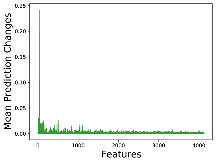
Figure 1: Feature sensitivity of EHR dataset

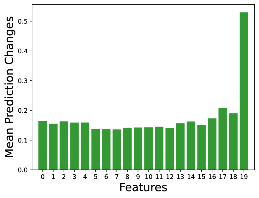
Figure 2: Feature sensitivity of IPS dataset

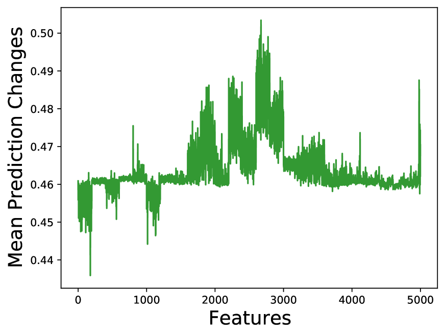
Figure 3: Feature sensitivity of PEDec dataset

Appendix E E.Parameter sensitivity analysis

We show below the variation of the attack performances using FEAT, with different settings of $\alpha$ in Eq.3. Adjusting the value of $\alpha$ balance exploration and exploitation in the search process. Larger $\alpha$ prefers exploration over the features that are not visited and modified before. On the contrary, smaller $\alpha$ biases the search process within the features that are considered to contribute high rewards.

Table 4: Attack performances of FEAT over the four datesets with different choices of $\alpha$

Dateset		Yelp-5		IPS		EHR		PEDec
Budget		6	8	5	6	4	6	10	12
$\alpha$ = 0	Runtime (sec)	0.11	0.24	0.56	0.74	0.86	0.38	8.98	9.36
	No.query	1293	2271	352	509	82.41	29.66	22618	23839
	SR	0.893	0.945	0.81	0.82	0.89	0.84	0.73	0.82
$\alpha$ = 2	Runtime (sec)	0.103	0.144	0.29	0.28	0.75	0.33	2.39	2.41
	No.query	662	911	113	112	71.28	24.70	7080	6607
	SR	0.95	0.96	0.92	0.93	0.89	0.899	0.75	0.87
$\alpha$ = 4	Runtime (sec)	0.101	0.143	0.28	0.28	0.74	0.32	4.10	4.13
	No.query	643	883	111	121	71.26	24.52	7080	6607
	SR	0.96	0.965	0.92	0.94	0.89	0.897	0.75	0.87
$\alpha$ = 8	Runtime	0.1	0.12	0.25	0.28	0.73	0.34	3.51	3.12
	No.query	632	883	119	123	54.59	20.45	7080	6607
	SR	0.954	0.965	0.93	0.92	0.932	0.935	0.75	0.87

From Table.4, we represent the performance metrics with $\alpha=0,2,4,8$ over four datasets. The bold set in each dataset have the rather better performance considering Runtime, No.query, SR together. PEDec (all the features sensitivity are almost the same level) need the smallest $\alpha$ to adjust the exploration, which means every feature you select in each iteration will contribute for the final reward and which dose not need deep exploration. Even you take the deep exploration $\alpha=8$, the attack performance results are almost the same as the condition $\alpha=2$. However, EHR and IPS (only one or a few features have the high features sensitivity) are suitable with the larger $\alpha=$ 4 and 8. Because the only one or a few features can make the main contribution to the adversarial attack, we explore these features in the whole features in the searching process. Especially if the whole feature number is very big, such as EHR with 4,130 features, this exploration will be more difficult.

Globally, on the datasets of severely skewed feature sensitivity distributions (like EHR and IPS), we prefer a large $\alpha$ to encourage exploration in the multi-armed bandit search over all of the features, so as to extend the exploration range to cover the rarely appearing yet highly sensitive features to guarantee the success of attack. In contrast, on the datasets of the uniformly distributed feature sensitivity level (like PEDec), we consider to choose a small $\alpha$ to put more weights on exploitation over the features empirically inducing larger variations than the others over the classifier’s decision confidence scores, in order to reach the attack goal within as few as possible iterations, i.e. improving the efficiency of the attack.

Appendix F F.Explanation to the adopted MAB setting

First, we show that adversarial attack over a categorical input $x_{i}$ is intrinsically a problem of set function maximization, following Eq.1 and Eq.4 on page 1 and 4 of (Hongyan et al. 2022).

Given an input instance ${x}=\{x_{1},x_{2},x_{3},...,x_{N}\}$ composed of $N$ categorical attributes, each $x_{i}$ can take any of optional ${M}$ categorical values. The classifier $f$ produces the soft decision scores $f_{y_{k}}$ ($k=1,2,3,...,{K}$) with respect to $K$ class labels. The goal of the attack is to find the minimal set of categorical feature perturbations $l=\texttt{diff}(x,\hat{{x}})$, with which the maximum gap between the decision score of any wrong label $k$ and the correct label ${K}$ is larger than 0.

$$\begin{split}&\hat{x}^{*}=\underset{\hat{{x}},\,\,l=\texttt{diff}({x},\hat{{x}})}{\operatorname*{arg\,max}}\quad m_{f}\\ &s.t.\quad m_{f}\geq{0},\,\;\;|l|\leq\varepsilon\end{split}$$ (43)

where $m_{f}=\underset{k\in\{1,...,{K}-1\}}{\max}\{f_{y_{k}}(\hat{x})\}-f_{y_{K}}(\hat{x})$ is the gap of the decision scores over the perturbed input instance $\hat{x}$. $m_{f}\in[-1,0)$ and $m_{f}\geq{0}$ correspond to correct and wrong classification output respectively. diff denotes the set of the perturbed categorical features in in the input instance $x$. $|\texttt{diff}|\leq{\epsilon}$ gives the budget limit of the attack. The number of the modified features in the attack should be no more than $\epsilon$. Different from the attacks with continuous data, solving the set function optimization problem requires to conduct a combinatorial search in the categorical feature space. This is in nature NP-hard. In the high-dimensional case, performing exhaustive search to solve Eq.1 is prohibitively expensive and randomly selecting features to perturb can produce arbitrarily bad results.

Relation between the reward definition and the set function maximization problem. In our study, the reward of modifying a categorical feature $x_{l}$ in the current iteration $t^{c}$ of the exploration process is defined as the maximum possible gap $m_{f}$ between any wrong label $k$ and the correct label $K$. We reorganize the formal definition of the reward value as in Eq.2.

$$\begin{split}G_{l,t^{c}}&=\underset{k=1,2,3,...,K-1}{\max}f_{y_{k}}(\hat{\mathbf{x}}_{t^{c}})-f_{y_{K}}(\hat{\mathbf{x}}_{t^{c}})+\Lambda\\ &\texttt{diff}(\hat{\mathbf{x}}_{t^{c}},\hat{\mathbf{x}}_{t^{c}-1})=\{x_{l}\}\\ \end{split}$$ (44)

where $\hat{\mathbf{x}}_{t^{c}}$ denotes the adversarially perturbed input instance at the current iteration $t^{c}$. $\texttt{diff}(\hat{\mathbf{x}}_{t^{c}},\hat{\mathbf{x}}_{t^{c}-1})=\{x_{l}\}$ denotes that only one more feature $x_{l}$ is changed at the current iteration $t^{c}$, compared to the previous iteration $t^{c}-1$. We add a large enough constant $\Lambda$, e.g. $\Lambda=1$ in practices, to ensure the non-negativeness of the received rewards.

The difference between the maximum reward derived at the two successive iterations $t^{c}$ and $t^{c}-1$ equals to the marginal gain of the set function maximization problem in Eq.1 by incrementally modifying one more feature.

$$\begin{split}&G^{*}_{t^{c}}-G^{*}_{t^{c}-1}=m_{f}(\hat{x}^{*}_{t^{c}})-m_{f}(\hat{x}^{*}_{t^{c}-1})\\ &G^{*}_{t^{c}}=\underset{x_{l}\in S^{t^{c}}}{max}\,\,G_{l,t^{c}}\\ &G^{*}_{t^{c}-1}=\underset{x_{l}\in S^{t^{c}-1}}{max}\,\,G_{l,t^{c}-1}\end{split}$$ (45)

where $S^{t^{c}}$ and $S^{t^{c}-1}$ are the sets of the candidate features at the iteration $t^{c}$ and $t^{c}-1$. $m_{f}(\hat{x}^{*}_{t^{c}})$ and $m_{f}(\hat{x}^{*}_{t^{c}})$ are the maximum $m_{f}$ value reached at the current iteration $t^{c}$ and its precedent iteration $t^{c}-1$. The difference between two maximum $m_{f}$ value defines the marginal gain of the maximization objective in Eq.1 by incrementally perturb one more feature of the input instance $x$.

Observation.1 The difference between the maximum rewards achieved at two successive iterations (in Eq.3) does not necessarily diminish for a general classifier $f$.

As a set function optimization problem, the marginal gain diminishes only if the set function-based objective follows the strict submodularity property (Elenberg et al. 2018), which further requires all the parameters of the target classifier to be positive (Qi et al. 2019; Elenberg et al. 2018). However, the positiveness constraint over the classifier’s parameters is not realistic and restricts severely the flexibility of the classifier. For a general classifier $f$, the submodularity of the corresponding attack objective (in Eq.1 of the revised submission) thus does not hold. As a result, the difference between the rewards received at successive iterations does not necessarily converge to zero along the search process. On the contrary, the reward difference given in Eq.45 can vary in a non-monotonically way.

This observation further implies the non-diminishing property of the reward value in the attack scenario against a general classifier. The reward difference given in Eq.45 can be considered as a relative effectiveness measurement of the perturbation efforts introduced at each iteration, compared to the last iteration. The larger the reward difference is, the more effective perturbation the current search iteration introduces compared to the previous iteration. In this sense, the non-monotonic variation of the reward difference indicates that the perturbation effects injected by modifying one more candidate feature does not diminish monotonically as the attack objective increases.

Observation.2 In the long run, we acknowledge that the reward distribution of changing one feature $x_{i}$ in the input is not stationary in general along the combinatorial search process. However, within the successive few iterations, the reward of modifying the top sensitive features does not commit significant drift. The rewards received by modifying these features remain stable within a few iterations of the combinatorial exploration.

For a classifier $f$ and a data set of testing input instances, we conduct one-factor-at-a-time sensitivity analysis (Campbell et al. 2008) over the categorical features. Given an input instance $x$, we change each feature $x_{i}$ while keeping all the others fixed. The averaged change of the probabilistic classification output over all the input instances in the data set is used as the feature-wise sensitivity measurement. A larger average change indicates that the classifier’s output is more sensitive to the change over the corresponding categorical feature.

Given the current iteration $t^{c}$, we measure the reward values received by modifying the top 10 sensitive features within the consecutive iterations $\{t^{c}+T\}$ ($T=0,1,2,3,4,...,6$). We then compute the ratio between the standard deviation and the average of the reward values by modifying each of the top 10 sensitive features $x_{l}$ within the consecutive iterations, noted as $\texttt{var}(\{G_{l,t^{c}+T}\})/\texttt{avg}(\{G_{l,t^{c}+T}\})$. The smaller the ratio $\texttt{var}(\{G_{l,t^{c}+T}\})/\texttt{avg}(\{G_{l,t^{c}+T}\})$ is, the more stable the reward of the corresponding feature $x_{l}$ stays across the consecutive iterations. We observe that all of the ratio values of the top 10 sensitive features remains lower than $1e^{-2}$ on the 4 datasets. In Figure.4, we take PEDec and EHR as the examples and show the value of $\texttt{var}(\{G_{l,t^{c}+T}\})/\texttt{avg}(\{G_{l,t^{c}+T}\})$ for the top-10 sensitive features on PEDec within the consecutive 6 UCB-based search iterations.

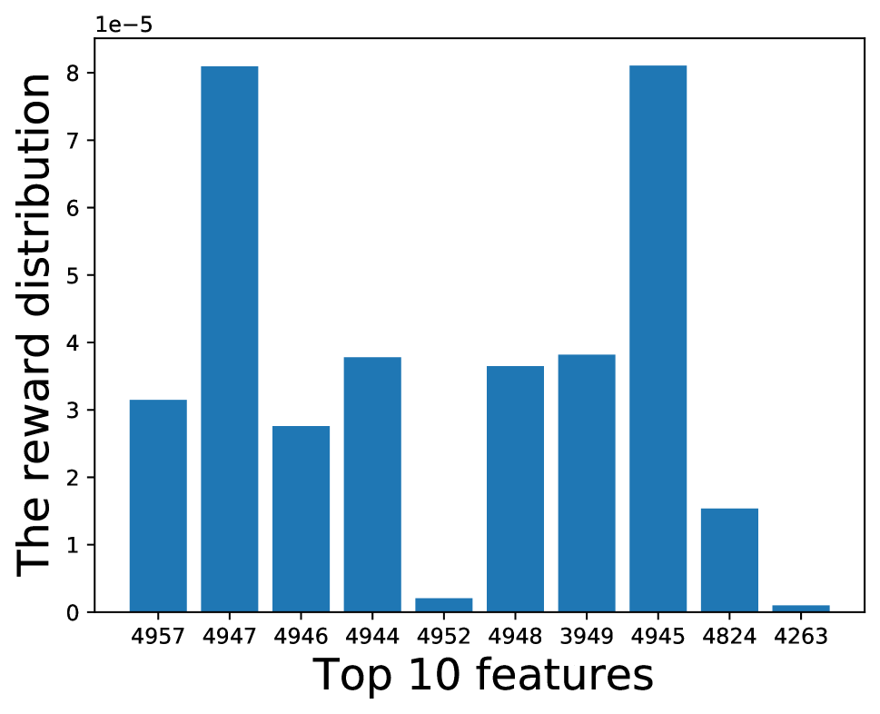
(a) PEDec

(b) EHR

Figure 4: The reward distribution of the top 10 sensitive features on PEDec and EHR.

The observations above denote that within the neighboring search iterations $\{t^{c}+T\}$. The variance of the rewards by perturbing those highly sensitive features is small. The potential explanation behind the observation can then be summarised as follows:

According to Theorem.1 in (Hongyan et al. 2022) (Eq.2 and 3 on Page 3 of (Hongyan et al. 2022)), the existence of the sensitive features is one of the key origins of adversarial vulnerability of the target classifier with categorical inputs. Higher feature sensitivity level causes significantly higher instability of the classifier’s decision output, if the sensitive features are perturbed. Therefore, even though the reward distribution of modifying one feature dimension may drift as more and more features are perturbed during the attack process, the impact of modifying these highly sensitive features over misleading the classifier’s decision remains relatively more stable than injecting modifications over other less sensitive features. Additionally, constraining the UCB-based search within the successive few iterations help further reduce the potential variation of the reward distribution in the search process.

Based on the observations, we adopt the following two-fold design in the proposed FEAT method to handle the non-stationary reward distribution during the search process:

First, we make use of the orthogonal matching pursuit (OMP) step in FEAT to select the features that can potentially bring the most variations to the classifier’s decision output. On IPS data set (1103 attributes), the 5 mostly selected features by the OMP step also appear as the top 20 sensitive features. On EHR data set (4130 attributes), the 7 most selected features by the OMP step show up in the top 20 sensitive features. The overlapping between the features useful for attack and the top ranked sensitive attributes indicates that using the OMP-guided exploration helps the attacker narrow down the combinatorial search range to focus on the most sensitive features.

Second, we apply the OMP step to compute the relaxed gradient magnitudes with respect to the candidate features after every $\tau$ UCB search iterations. We then re-initialise the UCB search over the updated top $L$ features that are re-selected by the OMP operation. In this sense, we adopt the UCB-based search in the inner iterations (see Line 6 to Line 16 of Algorithm.1 in the submission) and conduct the OMP operation in the outer iterations (see Line 3 to Line 5 of Algorithm.1 in the submission). In our experimental study, $\tau=5$ and $\tau=6$ both achieve the best empirical performances.

On one hand, we use the OMP operation in the outer iterations to restrict down the search range to the potentially sensitive features. The reward values with respect to those sensitive features tend to remain stable over different search rounds. On another hand, we reinitialize and relaunch the UCB-based search after the top $L$ features are updated in the outer iteration. Via this way, the proposed FEAT method constrains the UCB-based search within the consecutive $\tau$ inner iterations. Based on our observations, the reward distribution of the selected $L$ sensitive features can be considered empirically approximately stationary within the $\tau$ inner iterations.

fgithub

Appendix G G.Accuracy of the targeted classifier over adversary-free testing data

The testing accuracy with the targeted classifiers for different datesets is summarized in Table 5.

Table 5: This is the trained model of different dateset

Dataset	Classifier	Accuracy	F1	AUC
Yelp-5	LSTM	0.61	0.60	0.67
PEDec	CNN	0.94	0.92	0.90
IPS	LSTM	0.92	0.943	0.987
EHR	LSTM	0.932	0.883	0.909

In parallel to Table.2 in the submission, we provide the attack performance comparison of all the involved attack algorithms with the high attack budget in Table.6. Compared to Table.2, a higher attack budget level allows the attack methods to introduce more modifications to the input test instances. Hence the attack success rate and the averaged number of changed features increase correspondingly for most of the attack methods in Table.6. However, we can find that the proposed FEAT method can consistently obtain higher SR and lower/similar No.change than the other attack baselines on Yelp-5, IPS and EHR data, and ranks the second on PEDec. Simultaneously, FEAT delivers successful attacks by costing only a small fraction of Runtime and No.query. The results confirm in a further step the merits of balancing exploration and exploitation in the attack over high-dimensional categorical data.

Table 6: The performances of the attack methods evaluated on efficiency metrics with higher attack budget than those given in Table.2: Runtime (average running time in seconds) and No.query (average no. of $f(\hat{\textbf{x}})$ evaluation), and effectiveness metrics: SR (success rate) on four datasets. The attack time limit $T_{L}$=1000 sec for these four datasets.

Yelp-5		Budget = 8
Attack Type & Algo.		Runtime (sec) $\downarrow$	No.query $\downarrow$	SR $\uparrow$
Domain Specific	TextBugger	1.43	28	0.75
	TextFooler	0.19	155	0.86
Black Box	FSGS	1.62	84000	0.95
	FEAT-B	0.13	2000	0.92
White Box	GradAttack	0.46	129514	0.85
	OMPGS	0.82	7000	0.96
	FEAT	0.12	883	0.97

(a) The results on Yelp-5 data

IPS		Budget = 6
Attack Type & Algo.		Runtime (sec) $\downarrow$	No.query $\downarrow$	SR $\uparrow$
Black Box	FSGS	56.2	70000	0.85
	FEAT-B	19.5	2800	0.75
White Box	GradAttack	23.7	2500	0.75
	OMPGS	0.99	92.1	0.83
	FEAT	0.28	121	0.94

(b) The results on IPS data

References

- Agrawal and Goyal (2013) Agrawal, S.; and Goyal, N. 2013. Further Optimal Regret Bounds for Thompson Sampling. In Carvalho, C. M.; and Ravikumar, P., eds., Proceedings of the Sixteenth International Conference on Artificial Intelligence and Statistics, volume 31 of Proceedings of Machine Learning Research, 99–107. Scottsdale, Arizona, USA: PMLR.
- Asghar (2016) Asghar, N. 2016. Yelp dataset challenge: Review rating prediction. arXiv preprint arXiv:1605.05362.