Determinantal random subgraphs

Abstract.

We define two natural families of determinantal random subgraphs of a finite connected graph, one supported by acyclic spanning subgraphs (spanning forests) with fixed number of components, the other by connected spanning subgraphs with fixed number of independent cycles. Each family generalizes the uniform spanning tree and the generating functions of these probability measures generalize the classical Kirchhoff and Symanzik polynomials. We emphasize the matroidal nature of this construction, as well as possible generalisations.

Introduction

Since the work of Kirchhoff [Kir47], algebraic properties of spanning trees on finite connected graphs have kept fascinating and being rediscovered in various guises using a variety of techniques. They are ubiquitous in large areas of the literature in combinatorics, mathematical physics, probability, and linear algebra. Important foundational works of Whitney [Whi35] and Tutte [Tut54], followed by many others, have shown how fundamental these objects are in combinatorics, and also how they can be seen in a broader context, notably that of matroids. This point of view percolated in probability theory, notably through the work of Lyons [Lyo03].

It is known since the work of Burton and Pemantle [BP93, transfer current theorem] that the uniform probability measure on the set of spanning trees of a finite connected graph is a determinantal point process, a class of processes first introduced by Macchi [Mac75] and named that way by Borodin and Olshanski at the turn of the century, see [Bor11]. This measure had been studied earlier, in particular in relation to the Markov chain tree theorem (see [Ald90] and references therein), and extended to infinite graphs in [Pem91, BLPS01]; see the textbook [LP16]. In the planar case, the study of its scaling limit led Schramm to the discovery of SLE, see [Sch00, LSW04]. Analogs of uniform spanning trees on higher dimensional simplicial complexes were defined by Lyons [Lyo09], who also highlighted why the support of a determinantal probability measure is the same thing as the set of bases of a linear matroid. Later, Kenyon [Ken11] defined a determinantal probability measure on the set of cycle-rooted spanning forests of a graph, determined by a $1$-form on the graph. There are quaternion determinant analogs of these probability measures [Kas15, KL19].

On a graph, spanning trees and cycle-rooted spanning forests are the set of bases of the circular and bicircular matroids, respectively [Oxl11]. The circular case is the one from which the theory of matroids arose in the first place, whereas the bicircular case was only discovered later in [SP72] and further studied in [Mat77]. These are moreover the only matroids on the set of edges of a graph for which the set of circuits consists in all subgraphs homeomorphic to a given family of connected graphs [SP72].

The purpose of the present paper is to describe new families of determinantal probability measures on graphs, yielding random subgraphs with more complicated topology than trees, and an explicit geometric formula for the weight of each graph appearing in the associated partition function. This is the content of Theorems 4.3 and 4.6. The partition functions of these probability measures generalize the classical Symanzik and Kirchhoff polynomials (see Section 5). Moreover, we generalize these results to the case of linear matroids in Theorem 6.17 and suggest some possible further specializations of this theorem in Section 6.10.

Let us explain the content of Theorem 4.3. On a weighted graph $(\mathsf{G},\underline{x})$, given an integer $k\geq 0$, we consider the set $\mathcal{C}_{k}(\mathsf{G})$ of connected spanning subgraphs with exactly $k$ linearly independent cycles. Let us choose linearly independent $1$-forms $\theta_{1},\ldots,\theta_{k}$ which span a subspace that does not contain any non-zero exact $1$-form. For every $K\in\mathcal{C}_{k}(\mathsf{G})$, we choose an integral basis $(\gamma_{1},\ldots,\gamma_{k})$ of the free abelian group of cycles of $K$ and assign to $K$ the weight

$$w(K)=\big{|}\det\big{(}\theta_{i}(\gamma_{j})\big{)}_{1\leq i,j\leq k}\big{|}^{2}\ \underline{x}^{K},\,$$

where $\theta(\gamma)=\sum_{e\in\gamma}\theta_{e}$ and $\underline{x}^{K}$ is the product of the weights of the edges of $K$. We prove that the corresponding probability measure is determinantal, associated with the orthogonal projection on the direct sum of the space of exact $1$-forms and the span of $\theta_{1},\ldots,\theta_{k}$.

Our main tools for proving these results are an exterior algebra version of the matrix-tree theorem (Propositions 2.1, 2.4, and 6.4), and consequences of it, and the mean projection theorem for determinantal point processes (Theorem 3.2). The latter theorem was proven in [KL19, Theorem 5.9] and another proof was given in [KL22a]; earlier instances of special cases of this statement appeared in [NS61], [Mau76, Theorem 1], [Big97, Proposition 7.3], [Lyo03, Proposition 6.8], and [CCK13, CCK15, Theorem A].

Our approach allows us to unify the presentation of several statements concerning spanning trees (Sections 1 and 2), the Jacobian torus (Section 2.3), duality (Section 4.5) and complexes (Section 4.6), the Kirchhoff and Symanzik polynomials (Section 5), determinantal probability measures (Sections 3 and 6), cycle-rooted spanning forests (Section 6.10) and matroids (Section 6). Incidentally, it also yields a new formula for the probability density of a determinantal process (Proposition 6.8) and its restrictions (Corollary 6.11), in addition to the description of the above-mentioned families of examples of determinantal random subgraphs. In that respect, this paper also provides yet another, almost self-contained, presentation of these classical topics, expressed in the unifying language of exterior algebra.

The paper is organized as follows. In Section 1 we introduce some basic definitions about graphs and associated objects (chains, cochains, cycles, cuts, and integral bases determined by spanning trees). In Section 2, we review combinatorial multilinear identities involving spanning trees. In Section 3, we introduce four independent tools from the theory of determinantal probability measures and determinant computations. In Section 4 we show the existence of noteworthy determinantal probability measures on two families of subgraphs of constrained Betti numbers, which generalize the uniform measure on spanning trees. In Section 5, we make the connection to multivariate homogeneous polynomials from theoretical physics and derive a few consequences. Finally, in Section 6 we explain how the results presented extend from the circular matroid case to the general case of linear matroids, which in particular encompasses the case of the bicircular matroid, or ‘circular’ and ‘bicircular’ matroids on the set of cells of higher dimensional simplicial complexes.

Acknowledgements

We thank Omid Amini for inspiring discussions during work visits in Paris and Lyon on the topic of Symanzik polynomials and related structures. In particular, we realized while completing this work, which was motivated by different considerations in [KL22b], that the natural generalization of Symanzik polynomials we encounter here (see (50) in Section 5) had already been imagined by him several years ago, in the guise of the determinantal expression in the right-hand side of Proposition 4.5, based on the abstract construction of these polynomials in [ABBGF16, Section 2.1]. This paper thus also provides an answer to the question of Omid Amini of providing a concrete description and some properties of these polynomials. We also thank Javier Fresán for conversations at ETH Zurich which introduced us to [ABBGF16] back in 2015.

1. Spanning trees, cycles, and cuts

Most of what follows in this section is already known, but not presented exactly in that way; see for instance [Big74, Big97, BdlHN97].

Throughout the paper we will perform computations in the exterior algebra. For definitions and notations we refer to [KL19, Section 5].

1.1. Graphs and orientations

We denote by $\mathsf{G}=({\sf V},{\sf E})$ a finite connected graph, where ${\sf V}$ is the set of vertices, and ${\sf E}$ the set of edges, which we assume come with both possible orientations. Given an edge $e\in{\sf E}$, we let $\underline{e}$ and $\overline{e}$ be its starting and ending vertices, and let $e^{-1}$ be its inverse. We let $[{\sf E}]$ be the set of pairs $[e]=\{e,e^{-1}\}$, which we call geometric edges.

For a subgraph $S$ of $\mathsf{G}$, we denote by ${\sf V}(S)$ and ${\sf E}(S)$ its set of vertices and edges respectively; each edge of $S$ appears with both orientations in ${\sf E}(S)$. A subgraph needs not be connected, and can have isolated vertices.

A subgraph $S$ is said to be spanning when ${\sf V}(S)={\sf V}$. A spanning tree of $\mathsf{G}$ is a connected spanning subgraph which is minimal for inclusion. We denote by $\mathcal{T}(\mathsf{G})$ the set of spanning trees of $\mathsf{G}$.

We fix an orientation of $\mathsf{G}$, that is, a subset ${\sf E}^{+}$ of ${\sf E}$ containing exactly one element of each pair $\{e,e^{-1}\}$. Given a subgraph $S$ of $\mathsf{G}$, we will write ${\sf E}^{+}\setminus S$ for ${\sf E}^{+}(\mathsf{G})\setminus{\sf E}(S)$. Moreover, we will write $S^{+}$ for the directed graph whose vertex set is ${\sf V}$ and edge set is ${\sf E}^{+}(S)={\sf E}^{+}\cap{\sf E}(S)$.

1.2. Chains and cochains

Let us denote by $C_{0}(\mathsf{G},\mathbb{Z})$ the free $\mathbb{Z}$-module over the set ${\sf V}$ of vertices of our graph, and by $C_{1}(\mathsf{G},\mathbb{Z})$ the quotient of the free $\mathbb{Z}$-module over ${\sf E}$ by the submodule generated by $\{e+e^{-1}:e\in{\sf E}\}$. The classes of the elements of ${\sf E}^{+}$ form a basis of $C_{1}(\mathsf{G},\mathbb{Z})$, that we call the canonical basis, and we use this basis to identify $C_{1}(\mathsf{G},\mathbb{Z})$ with $\mathbb{Z}^{{\sf E}^{+}}$.

In order to be able to write matrices, we pick once and for all an arbitrary total ordering of ${\sf E}^{+}$. In particular, exterior products over sets of oriented edges will always be taken in this order.

The boundary operator $\partial:C_{1}(\mathsf{G},\mathbb{Z})\to C_{0}(\mathsf{G},\mathbb{Z})$ is defined by $\partial e=\overline{e}-\underline{e}$ and we define the group of cycles as

$$Z_{1}(\mathsf{G},\mathbb{Z})=\ker\partial.$$

The groups of cochains are defined by

$$C^{0}(\mathsf{G},\mathbb{Z})={\rm Hom}(C_{0}(\mathsf{G},\mathbb{Z}),\mathbb{Z})\ \ \text{ and }\ \ C^{1}(\mathsf{G},\mathbb{Z})={\rm Hom}(C_{1}(\mathsf{G},\mathbb{Z}),\mathbb{Z}).$$

We denote by $(\mathbbm{1}_{v})_{v\in{\sf V}}$ the canonical basis of $C^{0}(\mathsf{G},\mathbb{Z})$ and by $(e^{\star})_{e\in{\sf E}^{+}}$ the canonical basis of $C^{1}(\mathsf{G},\mathbb{Z})$. We have, for example, $e^{\star}(e^{-1})=-1$.

The pairing between chains and cochains is denoted by round brackets: for all chain $a$ and cochain $\alpha$ of the same degree, we write $(\alpha,a)=\alpha(a)$.

The coboundary operator $\delta:C^{0}(\mathsf{G},\mathbb{Z})\to C^{1}(\mathsf{G},\mathbb{Z})$ is the adjoint of the boundary operator, given by

$$\delta\mathbbm{1}_{v}=\sum_{e\in{\sf E}:\overline{e}=v}e^{\star}.$$

We define the group of cuts as

$$B^{1}(\mathsf{G},\mathbb{Z})=\mathop{\mathrm{im}}\delta.$$

1.3. Integral bases from spanning trees

In this section, the bases we refer to are bases of $\mathbb{Z}$-modules. We call them integral bases to distinguish them from bases of vector spaces that we consider later.

Let $T$ be a spanning tree of $\mathsf{G}$. To $T$, we associate two integral bases, respectively of $Z_{1}(\mathsf{G},\mathbb{Z})$ and $B^{1}(\mathsf{G},\mathbb{Z})$. Given two vertices $v,w$ of $\mathsf{G}$, we denote by $[v,w]_{T}$ the unique simple path from $v$ to $w$ in $T$, seen as an element of $C_{1}(\mathsf{G},\mathbb{Z})$.

Firstly, for each edge $f$, we define $\gamma(T,f)=f+[\overline{f},\underline{f}]_{T}\in Z_{1}(\mathsf{G},\mathbb{Z})$ to be the unique cycle created by adding $f$ to $T$. This cycle is oriented by $f$, and it is zero if and only $f$ belongs to $T$. It is well known (see for instance [Big74, Theorem 5.2]) that the family

$$\mathscr{Z}_{T}=\{\gamma(T,f):f\in{\sf E}^{+}\setminus T\}$$

is a basis of $Z_{1}(\mathsf{G},\mathbb{Z})$. Indeed, we have, for every cycle $c\in Z_{1}(\mathsf{G},\mathbb{Z})$ written as $c=\varepsilon_{1}e_{1}+\ldots+\varepsilon_{n}e_{n}$ with $\varepsilon_{1},\ldots,\varepsilon_{n}\in\{-1,1\}$ and $e_{1},\ldots,e_{n}\in{\sf E}^{+}$, the equality

(1) $$c=\varepsilon_{1}\gamma(T,e_{1})+\ldots+\varepsilon_{n}\gamma(T,e_{n}),$$

which follows from the fact that for all vertices $u,v,w$, the equality $[u,v]_{T}+[v,w]_{T}=[u,w]_{T}$ holds in $C_{1}(\mathsf{G},\mathbb{Z})$.

Secondly, for each edge $e$, we define $U(T,e)$ as the set of vertices of $\mathsf{G}$ that are connected to $\overline{e}$ in $T\setminus e$ and set

$$\kappa(T,e)=\delta(\mathbbm{1}_{U(T,e)})\in B^{1}(\mathsf{G},\mathbb{Z}).$$

The cut $\kappa(T,e)$ is zero if and only if $e$ does not belong to $T$ and the family

$$\mathscr{B}_{T}=\{\kappa(T,e):e\in T^{+}\}$$

is a basis of $B^{1}(\mathsf{G},\mathbb{Z})$ (this is also known, see for instance [BdlHN97]). Indeed, given an element $b=m_{1}e^{\star}_{1}+\ldots+m_{n}e^{\star}_{n}$ of $B^{1}(\mathsf{G},\mathbb{Z})$, we have

(2) $$b=m_{1}\kappa(T,e_{1})+\ldots+m_{n}\kappa(T,e_{n}).$$

This is because the difference between the two sides of this equation is an element of $B^{1}(\mathsf{G},\mathbb{Z})$ that is supported on ${\sf E}\setminus T$. It is thus of the form $\delta\eta$ for some $\eta\in C^{0}(\mathsf{G},\mathbb{Z})$ and since $T$ connects any two vertices of $\mathsf{G}$, the values of $\eta$ on any two vertices are equal. Thus, $\delta\eta=0$.

Whenever an order of the bases $\mathscr{Z}_{T}$ or $\mathscr{B}_{T}$ is needed, it will be that inherited from the total ordering on ${\sf E}^{+}$.

1.4. Projections on submodules

A spanning tree $T$ of $\mathsf{G}$ determines a splitting

(3) $$C_{1}(\mathsf{G},\mathbb{Z})=C_{1}(T,\mathbb{Z})\oplus Z_{1}(\mathsf{G},\mathbb{Z}),$$

according to the formula $f=-[\overline{f},\underline{f}]_{T}+\gamma(T,f)$ valid for each edge $f$. We denote by

(4) $${\sf Z}_{T}:C_{1}(\mathsf{G},\mathbb{Z})\to Z_{1}(\mathsf{G},\mathbb{Z}),\ f\mapsto\gamma(T,f)$$

the associated projection.

A spanning tree $T$ also determines a splitting

(5) $$C^{1}(\mathsf{G},\mathbb{Z})=B^{1}(\mathsf{G},\mathbb{Z})\oplus C^{1}(T^{c},\mathbb{Z}),$$

according to the decomposition $e^{\star}=\kappa(T,e)+(e^{\star}-\kappa(T,e))$. We denote by

(6) $$\mathsf{B}_{T}:C^{1}(\mathsf{G},\mathbb{Z})\to B^{1}(\mathsf{G},\mathbb{Z}),\ e^{\star}\mapsto\kappa(T,e)$$

the associated projection.

For every subgraph $S$, let us denote by $\pi_{S}:C_{1}(\mathsf{G},\mathbb{Z})\to C_{1}(S,\mathbb{Z})$ the projection corresponding to the decomposition $C_{1}(\mathsf{G},\mathbb{Z})=C_{1}(S,\mathbb{Z})\oplus C_{1}(S^{c},\mathbb{Z})$. We use the same notation for the projection $\pi_{S}:C^{1}(\mathsf{G},\mathbb{Z})\to C^{1}(S,\mathbb{Z})$ corresponding to the decomposition $C^{1}(\mathsf{G},\mathbb{Z})=C^{1}(S,\mathbb{Z})\oplus C^{1}(S^{c},\mathbb{Z})$.

For every spanning tree $T$ of $\mathsf{G}$, a rewriting of (1) and (2) yields the following equalities of endomorphisms, respectively of $Z_{1}(\mathsf{G},\mathbb{Z})$ and $B^{1}(\mathsf{G},\mathbb{Z})$:

(7) $${{\sf Z}}_{T}\circ\pi_{T^{c}}={\rm id}_{Z_{1}(\mathsf{G},\mathbb{Z})},$$

(8) $${\mathsf{B}}_{T}\circ\pi_{T}={\rm id}_{B^{1}(\mathsf{G},\mathbb{Z})}.$$

1.5. Inner products

Let us choose a base field $\mathbb{K}=\mathbb{R}$ or $\mathbb{C}$. We consider the spaces $\Omega^{0}(\mathsf{G})=C^{0}(\mathsf{G},\mathbb{Z})\otimes\mathbb{K}$ and $\Omega^{1}(\mathsf{G})=C^{1}(\mathsf{G},\mathbb{Z})\otimes\mathbb{K}$, consisting respectively in functions over the vertices, also called $0$-forms, and in antisymmetric functions over edges, also called $1$-forms.

We endow $\Omega^{0}(\mathsf{G})$ with the inner product

(9) $$\langle\langle f,g\rangle\rangle=\sum_{v\in{\sf V}}\overline{f_{v}}g_{v}.$$

We consider a collection $\underline{x}=(x_{e})_{e\in{\sf E}}$ of positive real weights on the edges of our graph, such that $x_{e^{-1}}=x_{e}$. We endow $\Omega^{1}(\mathsf{G})$ with the inner product

(10) $$\langle\langle\alpha,\beta\rangle\rangle=\sum_{e\in{\sf E}^{+}}x_{e}\,\overline{\alpha_{e}}\beta_{e}.$$

This definition is independent of the choice of orientation ${\sf E}^{+}$.

Note that the inner product (10) depends on $\underline{x}$, whereas (9) does not. In the following, we will not stress this dependence more explicitly, but it plays a key role in several proofs, where identities between polynomials in $\underline{x}$ are considered, see in particular Sections 3.2, 4, 5, and 6.

Every $1$-chain defines a linear form on $\Omega^{1}(\mathsf{G})$, that can be represented, thanks to the inner product on this space, by an element of $\Omega^{1}(\mathsf{G})$ itself. We denote by

(11) $${\sf J}_{\underline{x}}:C_{1}(\mathsf{G},\mathbb{Z})\otimes\mathbb{K}\to\Omega^{1}(\mathsf{G}),\ e\mapsto x_{e}^{-1}e^{\star}$$

this antilinear isomorphism. A similar but simpler antilinear isomorphism

(12) $${\sf J}^{0}:C_{0}(\mathsf{G},\mathbb{Z})\otimes\mathbb{K}\to\Omega^{0}(\mathsf{G}),\ v\mapsto\mathbbm{1}_{v}$$

exists, that does not depend on the inner product structure. For all $v\in{\sf V}$, $e\in{\sf E}$, $f\in\Omega^{0}(\mathsf{G})$ and $\alpha\in\Omega^{1}(\mathsf{G})$, the following relations hold:

(13) $$\langle\langle{\sf J}^{0}v,f\rangle\rangle=(f,v)=f(v)\ \ \text{and}\ \ \langle\langle{\sf J}_{\underline{x}}e,\alpha\rangle\rangle=(\alpha,e)=\alpha(e).$$

In the following, we will sometimes use adjoints of maps, denote $u^{*}$ for a map $u$, and this will be with respect to this weighted inner product (where the dependence on $x$ will be implicit in the notation).

For instance, we define $d=\delta\otimes{\rm id}_{\mathbb{K}}:\Omega^{0}(\mathsf{G})\to\Omega^{1}(\mathsf{G})$, the usual discrete differential, and its adjoint $d^{*}=\Omega^{1}(\mathsf{G})\to\Omega^{0}(\mathsf{G})$.

The operators $\partial$ and $d^{*}$ are related by the equation

(14) $${\sf J}^{0}\circ\partial=d^{*}\circ{\sf J}_{\underline{x}}.$$

Indeed, for all $e\in{\sf E}$, $f\in\Omega^{0}(\mathsf{G})$, we have $\langle\langle d^{*}{\sf J}_{\underline{x}}e,f\rangle\rangle=\langle\langle{\sf J}_{\underline{x}}e,df\rangle\rangle=(df,e)=(f,\partial e)=\langle\langle f,{\sf J}^{0}\partial e\rangle\rangle$.

1.6. Projections on subspaces

We have the orthogonal decomposition

(15) $$\Omega^{1}(\mathsf{G})=\mathop{\mathrm{im}}d\oplus\ker d^{*}\,.$$

On one hand, it follows from (14) that ${\sf J}_{\underline{x}}(Z_{1}(\mathsf{G},\mathbb{Z})\otimes\mathbb{K})=\ker d^{*}$. On the other hand, since $d=\delta\otimes{\rm id}_{\mathbb{K}}$, we simply have $\mathop{\mathrm{im}}d=B^{1}(\mathsf{G},\mathbb{Z})\otimes\mathbb{K}$.

Let $T\in\mathcal{T}(\mathsf{G})$ be a spanning tree. We have ${\sf J}_{\underline{x}}(C_{1}(T,\mathbb{Z})\otimes\mathbb{K})=\Omega^{1}(T)$, so that starting from (3), tensoring by $\mathbb{K}$ and applying ${\sf J}_{\underline{x}}$, we find

(16) $$\Omega^{1}(\mathsf{G})=\Omega^{1}(T)\oplus\ker d^{*}.$$

We denote by $\mathsf{P}^{\ker d^{*}}_{T}$ the associated projection on $\ker d^{*}$. According to the way in which we established the splitting, we have

(17) $$\mathsf{P}^{\ker d^{*}}_{T}={\sf J}_{\underline{x}}({\sf Z}_{T}\otimes{\rm id}_{\mathbb{K}}){\sf J}_{\underline{x}}^{-1}.$$

Starting from (5), we obtain simply by tensoring by $\mathbb{K}$ the splitting

(18) $$\Omega^{1}(\mathsf{G})=\mathop{\mathrm{im}}d\oplus\Omega^{1}(T^{c}).$$

Note that $\Omega^{1}(T^{c})$ is the orthogonal of $\Omega^{1}(T)$, independently of the choice of $\underline{x}$.

We denote by $\mathsf{P}^{\mathop{\mathrm{im}}d}_{T}$ the associated projection on $\mathop{\mathrm{im}}d$. We have

(19) $$\mathsf{P}^{\mathop{\mathrm{im}}d}_{T}=\mathsf{B}_{T}\otimes{\rm id}_{\mathbb{K}}.$$

1.7. Monomials and exterior powers

For any subgraph $S$ of $\mathsf{G}$ and for any collection of edges $A\subset{\sf E}(\mathsf{G})$, we define

$$\underline{x}^{S}=\prod_{e\in{\sf E}^{+}(S)}x_{e}\ \ \text{ and }\ \ \underline{x}^{A}=\prod_{e\in(A\cup A^{-1})\cap{\sf E}^{+}}x_{e}.$$

For every subgraph $S$, or every subset of edges, we denote by $e_{S}$ the exterior product of the positively oriented edges of $S$, taken in the order fixed in Section 1.2. Similarly, we denote by $e^{\star}_{S}$ the exterior product of the elements of the dual canonical basis of $C^{1}(\mathsf{G},\mathbb{Z})$ associated to the positively oriented edges of $S$, taken in the same order.

For every $k\geq 0$, the family $\{e^{\star}_{S}:S\subseteq{\sf E}^{+},|S|=k\}$ is orthogonal in $\mathchoice{\raisebox{1.0pt}{$\bigwedge$}}{\raisebox{1.0pt}{$\bigwedge$}}{\raisebox{0.5pt}{$\scriptstyle\bigwedge$}}{\raisebox{0.2pt}{$\scriptscriptstyle\bigwedge$}}^{k}C^{1}(\mathsf{G},\mathbb{Z})\otimes\mathbb{K}=\mathchoice{\raisebox{1.0pt}{$\bigwedge$}}{\raisebox{1.0pt}{$\bigwedge$}}{\raisebox{0.5pt}{$\scriptstyle\bigwedge$}}{\raisebox{0.2pt}{$\scriptscriptstyle\bigwedge$}}^{k}\Omega^{1}(\mathsf{G})$, and for each $S\subseteq{\sf E}^{+}$,

(20) $$\|e^{\star}_{S}\|^{2}=\underline{x}^{S}.$$

It will be useful to observe that if $S$ and $S^{\prime}$ are two subsets of ${\sf E}^{+}$, then $(\pi_{S})^{\wedge|S^{\prime}|}(e_{S^{\prime}})=e_{S^{\prime}}$ if $S^{\prime}\subseteq S$, and $0$ otherwise.

1.8. Edge weights and inner products: choice of convention

Let us make a comment about our choice of conventions for edge weights and inner products. We choose in this paper not to endow $\Omega_{1}(\mathsf{G})=C_{1}(\mathsf{G},\mathbb{Z})\otimes\mathbb{K}$, nor $\Omega_{0}(\mathsf{G})=C_{0}(\mathsf{G},\mathbb{Z})\otimes\mathbb{K}$ with any inner product. If we were to choose one, we would take the one which turns the maps ${\sf J}_{\underline{x}}$ and ${\sf J}^{0}$ into isometries.

The case of $\Omega_{0}(\mathsf{G})$ is of no surprise, since there is no dependency on $\underline{x}$ there. On $\Omega_{1}(\mathsf{G})=C_{1}(\mathsf{G},\mathbb{Z})\otimes\mathbb{K}$ this would be the inner product for which the canonical basis is orthogonal and for which $\|e\|^{2}=x_{e}^{-1}$ for every edge $e$. This may seem surprising for some readers, but we believe this is the most natural choice.

Under this inner product, for every $k\geq 0$, the family $\{e_{S}:S\subseteq{\sf E}^{+},|S|=k\}$ is orthogonal in $\mathchoice{\raisebox{1.0pt}{$\bigwedge$}}{\raisebox{1.0pt}{$\bigwedge$}}{\raisebox{0.5pt}{$\scriptstyle\bigwedge$}}{\raisebox{0.2pt}{$\scriptscriptstyle\bigwedge$}}^{k}C_{1}(\mathsf{G},\mathbb{Z})\otimes\mathbb{K}=\mathchoice{\raisebox{1.0pt}{$\bigwedge$}}{\raisebox{1.0pt}{$\bigwedge$}}{\raisebox{0.5pt}{$\scriptstyle\bigwedge$}}{\raisebox{0.2pt}{$\scriptscriptstyle\bigwedge$}}^{k}\Omega_{1}(\mathsf{G})$, and for each $S\subseteq{\sf E}^{+}$,

(21) $$\|e_{S}\|^{2}=(\underline{x}^{S})^{-1}.$$

2. Multilinear identities

Given two bases $\mathscr{B}_{1}$ and $\mathscr{B}_{2}$ of the same $\mathbb{Z}$-module, we will denote by $\det(\mathscr{B}_{1}/\mathscr{B}_{2})$ the determinant of the change of basis between $\mathscr{B}_{1}$ and $\mathscr{B}_{2}$, which is an element of $\{-1,1\}$. This element can be computed as follows: if $\mathscr{B}_{1}=(v_{1},\ldots,v_{r})$ and $\mathscr{B}_{2}=(w_{1},\ldots,w_{r})$, then

$$v_{1}\wedge\ldots\wedge v_{r}=\det(\mathscr{B}_{1}/\mathscr{B}_{2})\,w_{1}\wedge\ldots\wedge w_{r}.$$

We will use several times the following elementary fact: if a subgraph of $\mathsf{G}$ has the same number of edges as a spanning tree, that is, $|{\sf V}|-1$, without being a spanning tree itself, then this subgraph has at least one non-trivial cycle, and at least two connected components.

2.1. The Symanzik cycle-tree identity

The content of this section is somewhat related to a result of [ABKS14], although our statement and proof is different and elementary.

2.1.1. Spanning trees

Let us introduce the notation $b_{1}=b_{1}(\mathsf{G})$ for the rank of $Z_{1}(\mathsf{G},\mathbb{Z})$, called the first Betti number of $\mathsf{G}$. We have $b_{1}(\mathsf{G})=|{\sf E}^{+}|-|{\sf V}|+1$.

Proposition 2.1 (Cycle-tree identity).

Let $\mathscr{Z}=(\gamma_{1},\ldots,\gamma_{b_{1}})$ be a basis of $Z_{1}(\mathsf{G},\mathbb{Z})$. Then, in the free abelian group $\mathchoice{\raisebox{1.0pt}{$\bigwedge$}}{\raisebox{1.0pt}{$\bigwedge$}}{\raisebox{0.5pt}{$\scriptstyle\bigwedge$}}{\raisebox{0.2pt}{$\scriptscriptstyle\bigwedge$}}^{b_{1}}C_{1}(\mathsf{G},\mathbb{Z})$, we have

(22) $$\gamma_{1}\wedge\ldots\wedge\gamma_{b_{1}}=\sum_{T\in\mathcal{T}(\mathsf{G})}\det(\mathscr{Z}/\mathscr{Z}_{T})\,e_{T^{c}}.$$

Proof.

Let us decompose the element $\gamma_{1}\wedge\ldots\wedge\gamma_{b_{1}}$ of $\mathchoice{\raisebox{1.0pt}{$\bigwedge$}}{\raisebox{1.0pt}{$\bigwedge$}}{\raisebox{0.5pt}{$\scriptstyle\bigwedge$}}{\raisebox{0.2pt}{$\scriptscriptstyle\bigwedge$}}^{b_{1}}C_{1}(\mathsf{G},\mathbb{Z})$ on the basis $\{e_{S}:|S|=b_{1}\}$:

$$\gamma_{1}\wedge\ldots\wedge\gamma_{b_{1}}=\sum_{S\subset{\sf E}^{+}:|S|=b_{1}}a_{S}e_{S}.$$

Consider a subgraph $S$ with $b_{1}$ edges and assume that $S^{c}$ is not a spanning tree. Then $S^{c}$ contains a non-trivial cycle. This means that there exists a non-zero linear combination of $\gamma_{1},\ldots,\gamma_{b_{1}}$, say $\eta=n_{1}\gamma_{1}+\ldots+n_{b_{1}}\gamma_{b_{1}}$ that is supported by $S^{c}$. By reordering $\gamma_{1},\ldots,\gamma_{n}$ if needed, we make sure that $n_{1}\neq 0$. Then $0=(\pi_{S})^{\wedge b_{1}}(\eta\wedge\gamma_{2}\wedge\ldots\wedge\gamma_{b_{1}})=n_{1}(\pi_{S})^{\wedge b_{1}}(\gamma_{1}\wedge\ldots\wedge\gamma_{b_{1}})=n_{1}a_{S}e_{S}$, so that $a_{S}=0$.

Consider now a spanning tree $T$ of $\mathsf{G}$. Using (7), we find that

$$\gamma_{1}\wedge\ldots\wedge\gamma_{b_{1}}=({\sf Z}_{T}\circ\pi_{T^{c}})^{\wedge b_{1}}(\gamma_{1}\wedge\ldots\wedge\gamma_{b_{1}})=\sum_{S\subset{\sf E}^{+}:|S|=b_{1}}a_{S}\,({\sf Z}_{T})^{\wedge b_{1}}\big{(}(\pi_{T^{c}})^{\wedge b_{1}}(e_{S})\big{)}$$

and the only non-zero term of the last sum is that corresponding to $S=T^{c}$, so that

$$\gamma_{1}\wedge\ldots\wedge\gamma_{b_{1}}=a_{T^{c}}\,({\sf Z}_{T})^{\wedge b_{1}}e_{T^{c}}.$$

The result follows from the observation that $({\sf Z}_{T})^{\wedge b_{1}}e_{T^{c}}$ is the exterior product of the elements of the basis $\mathscr{Z}_{T}$. This identifies the coefficient $a_{T^{c}}$ as $\det(\mathscr{Z}/\mathscr{Z}_{T})$ and concludes the proof. ∎

Corollary 2.2.

For every spanning tree $T$ of $\mathsf{G}$, we have

(23) $$\pi_{T^{c}}(\gamma_{1})\wedge\ldots\wedge\pi_{T^{c}}(\gamma_{b_{1}})=\det(\mathscr{Z}/\mathscr{Z}_{T})\,e_{T^{c}}=\pm e_{T^{c}}.$$

Moreover, on $\mathchoice{\raisebox{1.0pt}{$\bigwedge$}}{\raisebox{1.0pt}{$\bigwedge$}}{\raisebox{0.5pt}{$\scriptstyle\bigwedge$}}{\raisebox{0.2pt}{$\scriptscriptstyle\bigwedge$}}^{b_{1}}Z_{1}(\mathsf{G},\mathbb{Z})$,

(24) $$\sum_{T\in\mathcal{T}(\mathsf{G})}\mathchoice{\raisebox{1.0pt}{$\bigwedge$}}{\raisebox{1.0pt}{$\bigwedge$}}{\raisebox{0.5pt}{$\scriptstyle\bigwedge$}}{\raisebox{0.2pt}{$\scriptscriptstyle\bigwedge$}}^{b_{1}}\pi_{T^{c}}={\rm id}.$$

Proof.

The first equality follows from applying $\mathchoice{\raisebox{1.0pt}{$\bigwedge$}}{\raisebox{1.0pt}{$\bigwedge$}}{\raisebox{0.5pt}{$\scriptstyle\bigwedge$}}{\raisebox{0.2pt}{$\scriptscriptstyle\bigwedge$}}^{b_{1}}\pi_{T^{c}}$ to (22) and using the fact that if $S$ and $T$ are spanning trees, then $\mathchoice{\raisebox{1.0pt}{$\bigwedge$}}{\raisebox{1.0pt}{$\bigwedge$}}{\raisebox{0.5pt}{$\scriptstyle\bigwedge$}}{\raisebox{0.2pt}{$\scriptscriptstyle\bigwedge$}}^{b_{1}}\pi_{T^{c}}(e_{S^{c}})=e_{S^{c}}$ if $S=T$ and $0$ otherwise.

The second equality follows from the first one, from (22), and the fact that $\mathchoice{\raisebox{1.0pt}{$\bigwedge$}}{\raisebox{1.0pt}{$\bigwedge$}}{\raisebox{0.5pt}{$\scriptstyle\bigwedge$}}{\raisebox{0.2pt}{$\scriptscriptstyle\bigwedge$}}^{b_{1}}Z_{1}(\mathsf{G},\mathbb{Z})$ is a module of rank $1$ generated by $\gamma_{1}\wedge\ldots\wedge\gamma_{b_{1}}$. ∎

2.1.2. Symanzik polynomial

It follows from an application of $\mathchoice{\raisebox{1.0pt}{$\bigwedge$}}{\raisebox{1.0pt}{$\bigwedge$}}{\raisebox{0.5pt}{$\scriptstyle\bigwedge$}}{\raisebox{0.2pt}{$\scriptscriptstyle\bigwedge$}}^{b_{1}}{\sf J}_{\underline{x}}$ to Proposition 2.1, Equation (20), and Pythagoras’ theorem in the Euclidean space $\mathchoice{\raisebox{1.0pt}{$\bigwedge$}}{\raisebox{1.0pt}{$\bigwedge$}}{\raisebox{0.5pt}{$\scriptstyle\bigwedge$}}{\raisebox{0.2pt}{$\scriptscriptstyle\bigwedge$}}^{b_{1}}C^{1}(\mathsf{G},\mathbb{Z})\otimes\mathbb{K}$ that

(25) $$\lVert{\sf J}_{\underline{x}}\gamma_{1}\wedge\ldots\wedge{\sf J}_{\underline{x}}\gamma_{b_{1}}\rVert^{2}=\sum_{T\in\mathcal{T}(\mathsf{G})}\;(\underline{x}^{-1})^{T^{c}}=(\underline{x}^{{\sf E}^{+}})^{-1}\sum_{T\in\mathcal{T}(\mathsf{G})}\;\underline{x}^{T}\,.$$

This can alternatively be phrased as follows: let $C=\mathrm{diag}(x_{e}:e\in{\sf E}^{+})$ be the diagonal matrix of weights $x_{e}$ and $M$ the $|{\sf E}^{+}|\times b_{1}$ matrix formed by writing the cycles $\gamma_{1},\ldots,\gamma_{b_{1}}$ in the canonical basis of $C_{1}(\mathsf{G},\mathbb{Z})$. Then

(26) $$\det({}^{t}\!MC^{-1}M)=\sum_{T\in\mathcal{T}(\mathsf{G})}\;(\underline{x}^{-1})^{T^{c}}\,,$$

an equality which appears in [Ami19, Lemma 3.1].

In the theory of Feynman integrals of Euclidean quantum field theory and associated graph polynomials [BW10], the right-hand side of (26) is called the first Symanzik polynomial (applied here to $\underline{x}^{-1}$ because of our conventions, see Section 1.8), so we propose to call (22) the Symanzik cycle-tree identity.

2.1.3. Connected subgraphs

Let us now turn to an application of Proposition 2.1. For each $k\in\{0,\ldots,b_{1}(\mathsf{G})\}$, let $\mathcal{C}_{k}(\mathsf{G})$ be the subset of connected spanning subgraphs with Betti number $k$, that is connected spanning subgraphs $K$ such that $Z_{1}(K,\mathbb{Z})$ has rank $k$ (i.e. $K$ has an excess of $k$ edges compared to the $|{\sf V}|-1$ edges of a spanning tree). In particular, we have $\mathcal{C}_{0}(\mathsf{G})=\mathcal{T}(\mathsf{G})$ and $\mathcal{C}_{b_{1}(\mathsf{G})}(\mathsf{G})=\{\mathsf{G}\}$.

Proposition 2.3.

Let $K\in\mathcal{C}_{k}(\mathsf{G})$ be a connected spanning subgraph. Let $(\gamma_{1},\ldots,\gamma_{k})$ be a basis of $Z_{1}(K,\mathbb{Z})$. Then in $\big{(}\mathchoice{\raisebox{1.0pt}{$\bigwedge$}}{\raisebox{1.0pt}{$\bigwedge$}}{\raisebox{0.5pt}{$\scriptstyle\bigwedge$}}{\raisebox{0.2pt}{$\scriptscriptstyle\bigwedge$}}^{k}Z_{1}(\mathsf{G},\mathbb{Z})\big{)}^{\otimes 2}$, we have

$$\sum_{\begin{subarray}{c}T\in\mathcal{T}(\mathsf{G})\\ T\subset K\end{subarray}}\mathchoice{\raisebox{1.0pt}{$\bigwedge$}}{\raisebox{1.0pt}{$\bigwedge$}}{\raisebox{0.5pt}{$\scriptstyle\bigwedge$}}{\raisebox{0.2pt}{$\scriptscriptstyle\bigwedge$}}^{k}{\sf Z}_{T}(e_{K\setminus T})\otimes e_{K\setminus T}=(\gamma_{1}\wedge\ldots\wedge\gamma_{k})^{\otimes 2}.$$

In more concrete terms, if for every spanning tree $T$ of $K$ we let $e_{1},\ldots,e_{k}$ be the positively oriented edges of $K\setminus T$, then

$$\sum_{T\in\mathcal{T}(K)}\left(\gamma(T,e_{1})\wedge\ldots\wedge\gamma(T,e_{k})\right)\otimes\left(e_{1}\wedge\ldots\wedge e_{k}\right)=(\gamma_{1}\wedge\ldots\wedge\gamma_{k})^{\otimes 2}.$$

Proof.

Let us compute the right-hand side of the equality to prove. We apply (24) on the graph $K$ to the second factor, and then the $k$-th exterior power of (7), also on the graph $K$, to each term of the sum, to find

$$(\gamma_{1}\wedge\ldots\wedge\gamma_{k})^{\otimes 2} =\sum_{T\in\mathcal{T}(K)}(\gamma_{1}\wedge\ldots\wedge\gamma_{k})\otimes\mathchoice{\raisebox{1.0pt}{$\bigwedge$}}{\raisebox{1.0pt}{$\bigwedge$}}{\raisebox{0.5pt}{$\scriptstyle\bigwedge$}}{\raisebox{0.2pt}{$\scriptscriptstyle\bigwedge$}}^{k}\pi_{T^{c}}(\gamma_{1}\wedge\ldots\wedge\gamma_{k})$$

$$=\sum_{T\in\mathcal{T}(K)}\mathchoice{\raisebox{1.0pt}{$\bigwedge$}}{\raisebox{1.0pt}{$\bigwedge$}}{\raisebox{0.5pt}{$\scriptstyle\bigwedge$}}{\raisebox{0.2pt}{$\scriptscriptstyle\bigwedge$}}^{k}{{\sf Z}}_{T}\circ\mathchoice{\raisebox{1.0pt}{$\bigwedge$}}{\raisebox{1.0pt}{$\bigwedge$}}{\raisebox{0.5pt}{$\scriptstyle\bigwedge$}}{\raisebox{0.2pt}{$\scriptscriptstyle\bigwedge$}}^{k}\pi_{T^{c}}(\gamma_{1}\wedge\ldots\wedge\gamma_{k})\otimes\mathchoice{\raisebox{1.0pt}{$\bigwedge$}}{\raisebox{1.0pt}{$\bigwedge$}}{\raisebox{0.5pt}{$\scriptstyle\bigwedge$}}{\raisebox{0.2pt}{$\scriptscriptstyle\bigwedge$}}^{k}\pi_{T^{c}}(\gamma_{1}\wedge\ldots\wedge\gamma_{k}).$$

For each spanning tree $T$ of $K$, an application of (23) gives $\pi_{T^{c}}(\gamma_{1}\wedge\ldots\wedge\gamma_{k})=\pm e_{K\setminus T}$ and the result follows. ∎

2.2. The Kirchhoff cut-tree identity

In this section, we consider the ‘dual case’ of the preceding section, and as a byproduct we derive a more classical version of the matrix-tree theorem by a similar strategy.

2.2.1. Spanning trees

Proposition 2.4 (Cut-tree identity).

Let $\mathscr{B}=(\kappa_{1},\ldots,\kappa_{|{\sf V}|-1})$ be an integral basis of $B^{1}(\mathsf{G},\mathbb{Z})$. In $\mathchoice{\raisebox{1.0pt}{$\bigwedge$}}{\raisebox{1.0pt}{$\bigwedge$}}{\raisebox{0.5pt}{$\scriptstyle\bigwedge$}}{\raisebox{0.2pt}{$\scriptscriptstyle\bigwedge$}}^{|{\sf V}|-1}C^{1}(\mathsf{G},\mathbb{Z})$, we have

(27) $$\kappa_{1}\wedge\ldots\wedge\kappa_{|{\sf V}|-1}=\sum_{T\in\mathcal{T}(\mathsf{G})}\det(\mathscr{B}/\mathscr{B}_{T})\,e^{\star}_{T}\;.$$

Proof.

Let us decompose $\kappa_{1}\wedge\ldots\wedge\kappa_{|{\sf V}|-1}\in\mathchoice{\raisebox{1.0pt}{$\bigwedge$}}{\raisebox{1.0pt}{$\bigwedge$}}{\raisebox{0.5pt}{$\scriptstyle\bigwedge$}}{\raisebox{0.2pt}{$\scriptscriptstyle\bigwedge$}}^{|{\sf V}|-1}C^{1}(\mathsf{G},\mathbb{Z})$ on the basis $\{e^{\star}_{S}:|S|=|{\sf V}|-1\}:$

$$\kappa_{1}\wedge\ldots\wedge\kappa_{|{\sf V}|-1}=\sum_{S\subset{\sf E}^{+}:|S|=|{\sf V}|-1}b_{S}e^{\star}_{S}.$$

Consider a subgraph $S$ with $|{\sf V}|-1$ edges that is not a spanning tree. Then $S$ has at least two connected components. Let $S_{1}$ be one of them. Then $\delta(\mathbbm{1}_{{\sf V}(S_{1})})$ is a non-zero element of $B^{1}(\mathsf{G},\mathbb{Z})$ that is supported by $S^{c}$. Thus, there is non-zero linear combination of $\kappa_{1},\ldots,\kappa_{|{\sf V}|-1}$, say $\alpha=n_{1}\kappa_{1}+\ldots+n_{|{\sf V}|-1}\kappa_{|{\sf V}|-1}$, that is supported by $S^{c}$. Reordering $\kappa_{1},\ldots,\kappa_{|{\sf V}|-1}$ if needed, we assume that $n_{1}\neq 0$. Then

$$0=(\pi_{S})^{\wedge(|{\sf V}|-1)}(\alpha\wedge\kappa_{2}\wedge\ldots\wedge\kappa_{|{\sf V}|-1})=n_{1}(\pi_{S})^{\wedge|{\sf V}|-1}(\kappa_{1}\wedge\ldots\wedge\kappa_{|{\sf V}|-1})=n_{1}b_{S}e^{\star}_{S},$$

so that $b_{S}=0$.

Consider now a spanning tree $T$ of $\mathsf{G}$. Using (8), we find that

$$\kappa_{1}\wedge\ldots\wedge\kappa_{|{\sf V}|-1}=(\mathsf{B}_{T}\circ\pi_{T})^{\wedge(|{\sf V}|-1)}(\kappa_{1}\wedge\ldots\wedge\kappa_{|{\sf V}|-1})=\sum_{S\subset{\sf E}^{+}:|S|=|{\sf V}|-1}b_{S}\,(\mathsf{B}_{T}\circ\pi_{T})^{\wedge|{\sf V}|-1}(e^{\star}_{S})$$

and the only non-zero term of the last sum is that corresponding to $S=T$, so that

$$\kappa_{1}\wedge\ldots\wedge\kappa_{|{\sf V}|-1}=b_{T}\,(\mathsf{B}_{T})^{\wedge(|{\sf V}|-1)}e^{\star}_{T}.$$

The result follows from the observation that $(\mathsf{B}_{T})^{\wedge(|{\sf V}|-1)}e^{\star}_{T}$ is the exterior product of the elements of the basis $\mathscr{B}_{T}$. This identifies the coefficient $b_{T}$ as $\det(\mathscr{B}/\mathscr{B}_{T})$ and concludes the proof. ∎

Corollary 2.5.

For every spanning tree $T$ of $\mathsf{G}$, we have

(28) $$\pi_{T}(\kappa_{1})\wedge\ldots\wedge\pi_{T}(\kappa_{|{\sf V}|-1})=\det(\mathscr{B}/\mathscr{B}_{T})\,e^{\star}_{T}=\pm e^{\star}_{T}.$$

Moreover, on $\mathchoice{\raisebox{1.0pt}{$\bigwedge$}}{\raisebox{1.0pt}{$\bigwedge$}}{\raisebox{0.5pt}{$\scriptstyle\bigwedge$}}{\raisebox{0.2pt}{$\scriptscriptstyle\bigwedge$}}^{|{\sf V}|-1}B^{1}(\mathsf{G},\mathbb{Z})$,

(29) $$\sum_{T\in\mathcal{T}(\mathsf{G})}\mathchoice{\raisebox{1.0pt}{$\bigwedge$}}{\raisebox{1.0pt}{$\bigwedge$}}{\raisebox{0.5pt}{$\scriptstyle\bigwedge$}}{\raisebox{0.2pt}{$\scriptscriptstyle\bigwedge$}}^{|{\sf V}|-1}\pi_{T}={\rm id}.$$

Proof.

The first equality follows from applying $\mathchoice{\raisebox{1.0pt}{$\bigwedge$}}{\raisebox{1.0pt}{$\bigwedge$}}{\raisebox{0.5pt}{$\scriptstyle\bigwedge$}}{\raisebox{0.2pt}{$\scriptscriptstyle\bigwedge$}}^{|{\sf V}|-1}\pi_{T}$ to (27) and using the fact that if $S$ and $T$ are spanning trees, then $\mathchoice{\raisebox{1.0pt}{$\bigwedge$}}{\raisebox{1.0pt}{$\bigwedge$}}{\raisebox{0.5pt}{$\scriptstyle\bigwedge$}}{\raisebox{0.2pt}{$\scriptscriptstyle\bigwedge$}}^{|{\sf V}|-1}\pi_{T}(e^{\star}_{S})=e^{\star}_{S}$ if $S=T$ and $0$ otherwise.

The second equality follows from the first one, from (27), and the fact that $\mathchoice{\raisebox{1.0pt}{$\bigwedge$}}{\raisebox{1.0pt}{$\bigwedge$}}{\raisebox{0.5pt}{$\scriptstyle\bigwedge$}}{\raisebox{0.2pt}{$\scriptscriptstyle\bigwedge$}}^{|V|-1}B^{1}(\mathsf{G},\mathbb{Z})$ is a module of rank $1$ generated by $\kappa_{1}\wedge\ldots\wedge\kappa_{|{\sf V}|-1}$. ∎

2.2.2. Kirchhoff polynomial

Applying Pythagoras’ theorem, as in Section 2.1.2, to both sides of the equality (27), we find

(30) $$\|\kappa_{1}\wedge\ldots\wedge\kappa_{|{\sf V}|-1}\|^{2}=\sum_{T\in\mathcal{T}(\mathsf{G})}\underline{x}^{T}\,.$$

The right-hand side of (30) is famously called the Kirchhoff polynomial and we hence propose to call (27) the Kirchhoff cut-tree identity.

To recover the classical matrix-tree theorem (see for instance [KL20]), we apply Proposition 2.4 to a special basis of $B^{1}(\mathsf{G},\mathbb{Z})$. To this end, we need to choose an ordering of the set ${\sf V}$ of vertices of $\mathsf{G}$. Let us fix a reference vertex $v_{0}$. Then $\mathscr{B}_{v_{0}}=\{\delta(\mathbbm{1}_{v}):v\in{\sf V}\setminus\{v_{0}\}\}$ is a basis of $B^{1}(\mathsf{G},\mathbb{Z})$. Then, using the notation $D$ of the proof, the matrix ${}^{t}\!DCD$ is the principal submatrix of the combinatorial Laplacian on $C^{0}(\mathsf{G},\mathbb{Z})$ where the row and column corresponding to $v_{0}$ have been erased. The equality (30) reads, in this case,

(31) $$\det({}^{t}\!DCD)=\sum_{T\in\mathcal{T}(\mathsf{G})}\underline{x}^{T}\,,$$

which is the most classical form of the matrix-tree theorem.

2.2.3. Spanning forests

As in Section 2.1, we now derive a consequence of Proposition 2.4.

For each $k\in\{1,\ldots,|{\sf V}|\}$, let $\mathcal{F}_{k}(\mathsf{G})$ denote the set of $k$-component spanning forests of $\mathsf{G}$. With this notation, note that $\mathcal{F}_{1}(\mathsf{G})=\mathcal{T}(\mathsf{G})$ and $\mathcal{F}_{|{\sf V}|}(\mathsf{G})=\{({\sf V},\varnothing)\}$.

For $F\in\mathcal{F}_{k}(\mathsf{G})$, we will consider the quotient graph $\mathsf{G}_{/F}$ obtained from $\mathsf{G}$ by contracting the edges of $F$. This graph has one vertex for each connected component of $F$, and its edges are the edges of $\mathsf{G}$ which join distinct connected components. Spanning trees of $\mathsf{G}_{/F}$ are the sets of edges of $\mathsf{G}$ which, when added to $F$, produce a spanning tree of $\mathsf{G}$.

We denote by $C^{0}(\mathsf{G}_{/F},\mathbb{Z})$ the submodule of $C^{0}(\mathsf{G},\mathbb{Z})$ consisting in the integer-valued functions on ${\sf V}$ that are constant on each connected component of $F$. We denote its image by $\delta$ by $B^{1}(\mathsf{G}_{/F},\mathbb{Z})\subseteq C^{1}(\mathsf{G},\mathbb{Z})$.

Proposition 2.6.

Let $F\in\mathcal{F}_{k+1}(\mathsf{G})$ be a spanning forest. Let $(\kappa_{1},\ldots,\kappa_{k})$ be a basis of $B^{1}(\mathsf{G}_{/F},\mathbb{Z})$. Then in $\big{(}\mathchoice{\raisebox{1.0pt}{$\bigwedge$}}{\raisebox{1.0pt}{$\bigwedge$}}{\raisebox{0.5pt}{$\scriptstyle\bigwedge$}}{\raisebox{0.2pt}{$\scriptscriptstyle\bigwedge$}}^{k}B^{1}(\mathsf{G},\mathbb{Z})\big{)}^{\otimes 2}$, we have

$$\sum_{\begin{subarray}{c}T\in\mathcal{T}(\mathsf{G})\\ T\supset F\end{subarray}}\mathchoice{\raisebox{1.0pt}{$\bigwedge$}}{\raisebox{1.0pt}{$\bigwedge$}}{\raisebox{0.5pt}{$\scriptstyle\bigwedge$}}{\raisebox{0.2pt}{$\scriptscriptstyle\bigwedge$}}^{k}{\sf B}_{T}(e^{\star}_{T\setminus F})\otimes e^{\star}_{T\setminus F}=(\kappa_{1}\wedge\ldots\wedge\kappa_{k})^{\otimes 2}.$$

In other words, if for every spanning tree $\tau$ of $\mathsf{G}_{/F}$ we let $e_{1},\ldots,e_{k}$ be its positively oriented edges, then

$$\sum_{\tau\in\mathcal{T}(\mathsf{G}_{/F})}\left(\kappa(F\cup\tau,e_{1})\wedge\ldots\wedge\kappa(F\cup\tau,e_{k})\right)\otimes\left(e^{\star}_{1}\wedge\ldots\wedge e^{\star}_{k}\right)=(\kappa_{1}\wedge\ldots\wedge\kappa_{k})^{\otimes 2}.$$

Proof.

Let us compute the right-hand side of the equality to prove. We apply (29) in the graph $\mathsf{G}_{/F}$ to the second factor, and then the $k$-th exterior power of the identity (8) to each term of the sum, to find

$$(\kappa_{1}\wedge\ldots\wedge\kappa_{k})^{\otimes 2} =\sum_{\tau\in\mathcal{T}(\mathsf{G}_{/F})}(\kappa_{1}\wedge\ldots\wedge\kappa_{k})\otimes\mathchoice{\raisebox{1.0pt}{$\bigwedge$}}{\raisebox{1.0pt}{$\bigwedge$}}{\raisebox{0.5pt}{$\scriptstyle\bigwedge$}}{\raisebox{0.2pt}{$\scriptscriptstyle\bigwedge$}}^{k}\pi_{\tau}(\kappa_{1}\wedge\ldots\wedge\kappa_{k})$$

$$=\sum_{\tau\in\mathcal{T}(\mathsf{G}_{/F})}\mathchoice{\raisebox{1.0pt}{$\bigwedge$}}{\raisebox{1.0pt}{$\bigwedge$}}{\raisebox{0.5pt}{$\scriptstyle\bigwedge$}}{\raisebox{0.2pt}{$\scriptscriptstyle\bigwedge$}}^{k}{\mathsf{B}}_{\tau}\circ\mathchoice{\raisebox{1.0pt}{$\bigwedge$}}{\raisebox{1.0pt}{$\bigwedge$}}{\raisebox{0.5pt}{$\scriptstyle\bigwedge$}}{\raisebox{0.2pt}{$\scriptscriptstyle\bigwedge$}}^{k}\pi_{\tau}(\kappa_{1}\wedge\ldots\wedge\kappa_{k})\otimes\mathchoice{\raisebox{1.0pt}{$\bigwedge$}}{\raisebox{1.0pt}{$\bigwedge$}}{\raisebox{0.5pt}{$\scriptstyle\bigwedge$}}{\raisebox{0.2pt}{$\scriptscriptstyle\bigwedge$}}^{k}\pi_{\tau}(\kappa_{1}\wedge\ldots\wedge\kappa_{k}).$$

For each spanning tree $\tau$ of $\mathsf{G}_{/F}$, applying (28) gives $\pi_{\tau}(\kappa_{1}\wedge\ldots\wedge\kappa_{k})=\pm e^{\star}_{\tau}=\pm e^{\star}_{T\setminus F}$ and the result follows. ∎

2.3. Real tori and finite abelian groups

Recall Equations (25) and (30), and let us use the same notations. Using (30) and the fact that ${\sf J}_{\underline{x}}(Z_{1}(\mathsf{G},\mathbb{K}))=\ker d^{*}$ is orthogonal to $B^{1}(\mathsf{G},\mathbb{K})=\mathop{\mathrm{im}}d$, we find

$$\|{\sf J}_{\underline{x}}\gamma_{1}\wedge\ldots\wedge{\sf J}_{\underline{x}}\gamma_{b_{1}}\wedge\kappa_{1}\wedge\ldots\wedge\kappa_{|{\sf V}|-1}\|^{2} =\|{\sf J}_{\underline{x}}\gamma_{1}\wedge\ldots\wedge{\sf J}_{\underline{x}}\gamma_{b_{1}}\|^{2}\|\kappa_{1}\wedge\ldots\wedge\kappa_{|{\sf V}|-1}\|^{2}$$

$$=(\underline{x}^{{\sf E}^{+}})^{-1}\,\bigg{(}\sum_{T\in\mathcal{T}(\mathsf{G})}\;\underline{x}^{T}\bigg{)}^{2}\,.$$

On the other hand, taking the exterior product of (22), to which we apply $\mathchoice{\raisebox{1.0pt}{$\bigwedge$}}{\raisebox{1.0pt}{$\bigwedge$}}{\raisebox{0.5pt}{$\scriptstyle\bigwedge$}}{\raisebox{0.2pt}{$\scriptscriptstyle\bigwedge$}}^{b_{1}}{\sf J}_{\underline{x}}$, and (27), we find

$${\sf J}_{\underline{x}}\gamma_{1}\wedge\ldots\wedge{\sf J}_{\underline{x}}\gamma_{b_{1}}\wedge\kappa_{1}\wedge\ldots\wedge\kappa_{|{\sf V}|-1}=\sum_{T\in\mathcal{T}(\mathsf{G})}\pm(\underline{x}^{T^{c}})^{-1}\,e^{\star}_{T^{c}}\wedge e^{\star}_{T}=(\underline{x}^{{\sf E}^{+}})^{-1}\bigg{(}\sum_{T\in\mathcal{T}(\mathsf{G})}\pm\underline{x}^{T}\bigg{)}e^{\star}_{{\sf E}^{+}}\,.$$

Comparing with the previous equality, we deduce that all signs in the sum are the same. Thus, we have proved the following proposition.

Proposition 2.7.

Let $(\gamma_{1},\ldots,\gamma_{b_{1}})$ be a basis of $Z_{1}(\mathsf{G},\mathbb{Z})$ and $(\kappa_{1},\ldots,\kappa_{|V|-1})$ a basis of $B^{1}(\mathsf{G},\mathbb{Z})$. Then in the line $\mathchoice{\raisebox{1.0pt}{$\bigwedge$}}{\raisebox{1.0pt}{$\bigwedge$}}{\raisebox{0.5pt}{$\scriptstyle\bigwedge$}}{\raisebox{0.2pt}{$\scriptscriptstyle\bigwedge$}}^{|{\sf E}^{+}|}\Omega^{1}(\mathsf{G})$, we have

$${\sf J}_{\underline{x}}\gamma_{1}\wedge\ldots\wedge{\sf J}_{\underline{x}}\gamma_{b_{1}}\wedge\kappa_{1}\wedge\ldots\wedge\kappa_{|{\sf V}|-1}=\pm(\underline{x}^{{\sf E}^{+}})^{-1}\bigg{(}\sum_{T\in\mathcal{T}(\mathsf{G})}\underline{x}^{T}\bigg{)}e^{\star}_{{\sf E}^{+}}\,.$$

In particular,

$$\|{\sf J}_{\underline{x}}\gamma_{1}\wedge\ldots\wedge{\sf J}_{\underline{x}}\gamma_{b_{1}}\wedge\kappa_{1}\wedge\ldots\wedge\kappa_{|{\sf V}|-1}\|=(\underline{x}^{{\sf E}^{+}})^{-\frac{1}{2}}\,\sum_{T\in\mathcal{T}(\mathsf{G})}\;\underline{x}^{T}.$$

In the vector space $\Omega^{1}(\mathsf{G})$, the elements ${\sf J}_{\underline{x}}\gamma_{1},\ldots,{\sf J}_{\underline{x}}\gamma_{b_{1}},\kappa_{1},\ldots,\kappa_{|{\sf V}|-1}$ form a basis, and generate a lattice. This lattice, as a discrete abelian subgroup of $\Omega^{1}(\mathsf{G})$, does not depend on our choice of basis, indeed it is equal to ${\sf J}_{\underline{x}}(Z_{1}(\mathsf{G},\mathbb{Z}))\oplus B^{1}(\mathsf{G},\mathbb{Z})$. The quotient

$$C^{1}(\mathsf{G},\mathbb{R})/\big{(}{\sf J}_{\underline{x}}(Z_{1}(\mathsf{G},\mathbb{Z}))\oplus B^{1}(\mathsf{G},\mathbb{Z})\big{)}$$

is a real torus, of which the second assertion of the proposition computes the volume. In the case where all the weights $x_{e}$ are taken to be equal to $1$, this volume is equal to the number of spanning trees of $\mathsf{G}$.

Still in the case where $\underline{x}$ is identically equal to $\underline{1}$, this volume is equal to the cardinal of the finite group

$$C^{1}(\mathsf{G},\mathbb{Z})/\big{(}{\sf J}_{\underline{1}}(Z_{1}(\mathsf{G},\mathbb{Z}))\oplus B^{1}(\mathsf{G},\mathbb{Z})\big{)}.$$

Taking $\underline{x}$ identically equal to $\underline{1}$ blurs the distinction between chains and cochains and we can identify them. Then, we can write the last group as

$$C_{1}(\mathsf{G},\mathbb{Z})/\big{(}Z_{1}(\mathsf{G},\mathbb{Z})\oplus\delta C_{0}(\mathsf{G},\mathbb{Z})\big{)}.$$

The boundary map $\partial$ descends to an injective map on this quotient, and induces an isomorphism with the group

$$\partial C_{1}(\mathsf{G},\mathbb{Z})/\partial\delta C_{0}(\mathsf{G},\mathbb{Z}),$$

sometimes called the Jacobian group of the graph, itself isomorphic to the sandpile group

$$C_{0}(\mathsf{G}\setminus\{v_{0}\},\mathbb{Z})/\partial\delta C_{0}(\mathsf{G}\setminus\{v_{0}\},\mathbb{Z}),$$

where $v_{0}$ is an arbitrarily chosen vertex, see [CP18, Corollary 13.15] and [BdlHN97, Big99]. Kotani and Sunada also define the Jacobian torus [KS00], see also [ABKS14].

3. Determinantal toolbox

In this section, we collect four useful and fairly independent properties of determinantal probability measures and determinants.

3.1. Determinantal measures on finite sets

Let $(E,\langle\cdot,\cdot\rangle)$ be a finite-dimensional Euclidean space. Consider a linear subspace $H$ of $E$ and an orthonormal basis $(e_{i})_{i\in S}$ of $E$, indexed by some finite set $S$.

A random subset ${\mathsf{X}}$ of $S$ is determinantal associated to $H$ in the basis $(e_{i})_{i\in S}$ if for all subset $J\subseteq S$, we have

$$\mathbb{P}(J\subseteq{\mathsf{X}})=\det({\sf\Pi}^{H})_{E_{J}}^{E_{J}}$$

where ${\sf\Pi}^{H}$ is the orthogonal projection on $H$ and $({\sf\Pi}^{H})_{E_{J}}^{E_{J}}$ its compression on the coordinate subspace $E_{J}=\oplus_{i\in J}\mathbb{K}e_{i}$.

3.2. The routine construction lemma

The following lemma states that showing that a random subset is determinantal associated with a self-dual projection is equivalent to showing a matrix-tree type formula, as an equality of polynomial, where the name comes from the special case (31).

For each set of non-zero positive weights $\underline{x}=(x_{i})_{i\in S}$, we twist the inner product on $E$ by setting, for all $u,v\in E$,

(32) $$\langle u,v\rangle_{\underline{x}}=\sum_{i\in S}x_{i}\overline{u_{i}}v_{i}$$

where $(u_{i})_{i\in S}$ and $(v_{i})_{i\in S}$ are the coefficients of $u$ and $v$ in the basis $(e_{i})_{i\in S}$. Note that the basis $(e_{i})_{i\in S}$ is still orthogonal with respect to the twisted inner product (which takes the most general form of an inner product with this property).

Lemma 3.1.

Let $w:2^{S}\to\mathbb{R}^{*}_{+}$ be a map that is not identically zero. Let $a$ be an injective linear map from some inner product space into $E$. Assume that for all $\underline{x}\in(0,\infty)^{S}$, we have

(33) $$\det(a^{*}a)=\sum_{B\subseteq S}\underline{x}^{B}\;w(B)\,,$$

where $a^{*}$ is the adjoint of $a$ with respect to the twisted inner product (32) on $E$. Then, for any $\underline{x}\in(0,\infty)^{S}$, the probability measure on $2^{S}$ which assigns $B$ a probability

(34) $$\mathbb{P}(B)\propto\underline{x}^{B}w(B)$$

is determinantal, associated with the orthogonal projection on $\mathop{\mathrm{im}}a$, where orthogonality is defined with respect to the twisted scalar product (32).

Proof.

Let $\underline{y}\in(0,\infty)^{S}$ be another set of positive weights. Let $c_{\underline{y}}$ be the endomorphism of $E$ defined by $c_{\underline{y}}(e_{i})=y_{i}e_{i}$. Then the adjoint of $a$ with respect to the $\underline{xy}$-twisted inner product is $a^{*}c_{\underline{y}}$ where $a^{*}$ is the adjoint with respect to the $\underline{x}$-twisted inner product.

If the assumption (33) holds, then the generating function of the probability measure (34) is

(35) $$\sum_{B\subseteq S}\underline{y}^{B}\;\mathbb{P}(B)=\frac{\sum_{B\subseteq S}\underline{y}^{B}\underline{x}^{B}w(B)}{\sum_{B\subseteq S}\underline{x}^{B}w(B)}=\frac{\det(a^{*}c_{\underline{y}}a)}{\det(a^{*}a)}\,.$$

On the other hand, according to [Lyo03], or [KL19], the generating function of the determinantal measure on $2^{S}$ associated to ${\sf\Pi}^{\mathop{\mathrm{im}}a}=a(a^{*}a)^{-1}a^{*}$ is

$$\det(\mathrm{id}+(c_{\underline{y}}-\mathrm{id}){\sf\Pi}^{\mathop{\mathrm{im}}a}) =\det(\mathrm{id}+(c_{\underline{y}}-\mathrm{id})a(a^{*}a)^{-1}a^{*})$$

$$=\det(\mathrm{id}+a^{*}(c_{\underline{y}}-\mathrm{id})a(a^{*}a)^{-1})$$

$$=\det(a^{*}c_{\underline{y}}a)/\det(a^{*}a),$$

and the second assertion is proved. ∎

3.3. A variant of the mean projection theorem

For a vector space $E$ written as the direct sum of two subspaces $F$ and $H$, we write $\mathsf{P}^{F}_{\parallel H}$ for the projection of $E$ onto $F$ parallel to $H$. We however keep the notation ${\sf\Pi}^{F}$ when $F$ is the orthogonal of $H$ with respect to an inner product.

We use the notation $\mathchoice{\raisebox{1.0pt}{$\bigwedge$}}{\raisebox{1.0pt}{$\bigwedge$}}{\raisebox{0.5pt}{$\scriptstyle\bigwedge$}}{\raisebox{0.2pt}{$\scriptscriptstyle\bigwedge$}}\mathsf{a}$ for the endomorphism of the exterior algebra $\mathchoice{\raisebox{1.0pt}{$\bigwedge$}}{\raisebox{1.0pt}{$\bigwedge$}}{\raisebox{0.5pt}{$\scriptstyle\bigwedge$}}{\raisebox{0.2pt}{$\scriptscriptstyle\bigwedge$}}E$ of $E$ induced by an operator $\mathsf{a}\in\mathrm{End}(E)$ (see [KL19, Section 5.4]).

Let $E$ be a finite-dimensional inner product space and $(e_{i})_{i\in S}$ be an orthonormal basis of $E$.

Theorem 3.2.

Let $H$ be a linear subspace of $E$. Let ${\mathsf{X}}$ be the determinantal random subset of $S$ associated with ${\sf\Pi}^{H}$ in the orthonormal basis $(e_{i})_{i\in S}$, and let $E_{{\mathsf{X}}}=\oplus_{x\in{\mathsf{X}}}\mathbb{K}e_{x}$. Then

$$\mathchoice{\raisebox{1.0pt}{$\bigwedge$}}{\raisebox{1.0pt}{$\bigwedge$}}{\raisebox{0.5pt}{$\scriptstyle\bigwedge$}}{\raisebox{0.2pt}{$\scriptscriptstyle\bigwedge$}}{\sf\Pi}^{H^{\perp}}=\mathbb{E}\big{[}\mathchoice{\raisebox{1.0pt}{$\bigwedge$}}{\raisebox{1.0pt}{$\bigwedge$}}{\raisebox{0.5pt}{$\scriptstyle\bigwedge$}}{\raisebox{0.2pt}{$\scriptscriptstyle\bigwedge$}}\mathsf{P}^{H^{\perp}}_{\parallel E_{{\mathsf{X}}}}\big{]}\,.$$

Proof.

We apply [KL19, Theorem 5.9] to the determinantal subset of $S$ associated with ${\sf\Pi}^{H^{\perp}}$ and use the fact, proved in [KL19, Proposition 4.2], that ${\mathsf{X}}$ is the complement of this determinantal subset. ∎

3.4. Conditional probability measure

The following result will only be needed in Section 6.6, but we record it here for future reference.

Lemma 3.3.

Let $H$ be a linear subspace of $E$. Let ${\mathsf{X}}$ be the determinantal random subset of $S$ associated with ${\sf\Pi}^{H}$ in the orthonormal basis $(e_{i})_{i\in S}$. Let $K\subset S$ be such that $\mathbb{P}({\mathsf{X}}\subset K)>0$. Then the random subset ${\mathsf{X}}$ conditioned on staying inside $K$ is distributed according to the determinantal probability measure on $2^{K}$ associated with the orthogonal projection on the subspace ${\sf\Pi}^{E_{K}}(H)$, where $E_{K}=\oplus_{i\in K}\mathbb{K}e_{i}$.

Note that the assumption $\mathbb{P}({\mathsf{X}}\subset K)>0$ is equivalent to $E_{K^{c}}\cap H=\{0\}$, or $E_{K}+H^{\perp}=E$.

Proof.

The gist of the proof is to use Pythagoras’ theorem in the $n$-th exterior power of $E$ in an associative way. More precisely, let us denote by $\iota_{H}$ a normed Plücker embedding of $H$, that is, the exterior product of the elements of an orthonormal basis of $H$. This vector is uniquely defined only up to a sign (when $\mathbb{K}=\mathbb{R})$ or a phase (when $\mathbb{K}=\mathbb{C}$).

For all $T=\{i_{1},\ldots,i_{n}\}$, set $e_{T}=e_{i_{1}}\wedge\ldots\wedge e_{i_{n}}$. Then, summing only over subsets of $S$ of cardinality $n$, we have

$$1=\lVert\iota_{H}\rVert^{2} =\sum_{T}|\langle\iota_{H},e_{T}\rangle|^{2}=\sum_{T\subset K}|\langle\iota_{H},e_{T}\rangle|^{2}+\sum_{T\cap K^{c}\neq\varnothing}|\langle\iota_{H},e_{T}\rangle|^{2}\,.$$

The first sum of the above right-hand side is equal to $\mathbb{P}({\mathsf{X}}\subset K)$, which is positive by assumption. It is also equal to $\lVert{\sf\Pi}^{\mathchoice{\raisebox{1.0pt}{$\bigwedge$}}{\raisebox{1.0pt}{$\bigwedge$}}{\raisebox{0.5pt}{$\scriptstyle\bigwedge$}}{\raisebox{0.2pt}{$\scriptscriptstyle\bigwedge$}}^{n}E_{K}}(\iota_{H})\rVert^{2}$. We also observe that $\iota_{H}^{K}={\sf\Pi}^{\mathchoice{\raisebox{1.0pt}{$\bigwedge$}}{\raisebox{1.0pt}{$\bigwedge$}}{\raisebox{0.5pt}{$\scriptstyle\bigwedge$}}{\raisebox{0.2pt}{$\scriptscriptstyle\bigwedge$}}^{n}E_{K}}(\iota_{H})/\lVert{\sf\Pi}^{\mathchoice{\raisebox{1.0pt}{$\bigwedge$}}{\raisebox{1.0pt}{$\bigwedge$}}{\raisebox{0.5pt}{$\scriptstyle\bigwedge$}}{\raisebox{0.2pt}{$\scriptscriptstyle\bigwedge$}}^{n}E_{K}}(\iota_{H})\rVert$ is a normed Plücker embedding of ${\sf\Pi}^{E_{K}}(H)$ in $\mathchoice{\raisebox{1.0pt}{$\bigwedge$}}{\raisebox{1.0pt}{$\bigwedge$}}{\raisebox{0.5pt}{$\scriptstyle\bigwedge$}}{\raisebox{0.2pt}{$\scriptscriptstyle\bigwedge$}}^{n}E_{K}$.

Thus, for all $T\subset K$, we have

$$\mathbb{P}\big{(}{\mathsf{X}}=T\,\big{|}\,{\mathsf{X}}\subset K\big{)}=|\langle\iota_{H}^{K},e_{T}\rangle|^{2}$$

which proves the claim. ∎

3.5. Schur complement

We use the following notation: for every subspace $H$ of an inner product space $E$, we denote by $1_{H}$ the inclusion of $H$ in $E$ and $1^{H}$ its adjoint, that is, the orthogonal projection on $H$.

Lemma 3.4.

Let $u:E_{0}\to E_{1}$ be an injective linear map between finite-dimensional inner product spaces. Let $H$ be a subspace of $E_{0}$. Then

$$\det(u^{*}u)=\det\left(1^{H^{\perp}}u^{*}u1_{H^{\perp}}\right)\det\left(1^{H}u^{*}{\sf\Pi}^{\ker(1^{H^{\perp}}u^{*})}u1_{H}\right)\,.$$

The determinant $\det(u^{*}u)$ is the square of the volume in $E_{1}$ of the image by $u$ of a unit parallelotope in $E_{0}$. This result expresses this volume as a product of two lower-dimensional volumes corresponding to a decomposition of $E_{0}$ in the sum of two orthogonal spaces.

Proof.

Let us start by writing

$$u=u1_{H^{\perp}}+u1_{H}\ \text{ and }\ u^{*}=1^{H^{\perp}}u^{*}+1^{H}u^{*}.$$

Using the Schur complement formula, we find

$$\det(u^{*}u) =\det\left(1^{H^{\perp}}u^{*}u1_{H^{\perp}}\right)\det\left(1^{H}u^{*}u1_{H}-1^{H}u^{*}u1_{H^{\perp}}(1^{H^{\perp}}u^{*}u1_{H^{\perp}})^{-1}1^{H^{\perp}}u^{*}u1_{H}\right)$$

$$=\det\left(1^{H^{\perp}}u^{*}u1_{H^{\perp}}\right)\det\left(1^{H}u^{*}\Big{[}\mathrm{id}_{E_{1}}-u1_{H^{\perp}}(1^{H^{\perp}}u^{*}u1_{H^{\perp}})^{-1}1^{H^{\perp}}u^{*}\Big{]}u1_{H}\right).$$

Between the square brackets, we have an operator $\mathrm{id}_{E_{1}}-p$, where $p$ is the orthogonal projection on the range of $u1_{H^{\perp}}$. Hence, this operator is the orthogonal projection on $\ker(1^{H^{\perp}}u^{*})$. ∎

4. Random spanning connected or acyclic subgraphs

We now introduce two families of determinantal probability measures on the bases of matroids obtained from the circular matroid either by adjoining $k$ edges, or removing $k$ edges. Later in Section 6.10 we extend these to a family of determinantal measures on subgraphs with constrained Betti numbers.

The random subgraphs are connected subgraphs or spanning forests with fixed Euler characteristics, see Figure 1.

In general, our probability measures are not uniform. In fact, in view of the complexity results stated below (see the last paragraph of Section 4.5), the uniform measure on $\mathcal{C}_{k}(\mathsf{G})$ and $\mathcal{F}_{k}(\mathsf{G})$ cannot be determinantal in general (otherwise there would be a determinantal formula for enumerating them, contradicting the $\#P$-hardness). Studying the uniform measure would be a more difficult task; on that matter, see [GW04] for conjectures about the uniform measure on connected subgraphs, or spanning forests, without constraint on the Betti numbers.

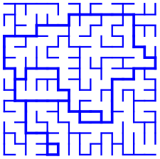
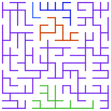
Figure 1. A random element of $\mathcal{C}_{4}(\mathsf{G})$ (its $2$-core is represented by thickened edges) and a random element of $\mathcal{F}_{5}(\mathsf{G})$ on a $15\times 15$ square grid determined by $4$ random $1$-forms. The sampling algorithm we used here, and for the other figures, is the classical one of [HKPV06, Algorithm 18] for sampling determinantal probability measures.

4.1. Determinantal random subgraphs

The general idea we describe now is how from subspaces of $\Omega^{1}(\mathsf{G})$ or $\Omega_{1}(\mathsf{G})$ it is possible to produce determinantal measures on $[{\sf E}]$ corresponding to geometric-topological ‘Boltzmann weights’ on the families of subgraphs. The procedure involves the pairing of $\mathbb{K}$-valued $1$-chains or $1$-forms taken in theses subspaces with special $\mathbb{Z}$-valued $1$-chains or $1$-cochains built from integral bases of $\mathbb{Z}$-modules determined by the subgraph.

Specializing the definition of Section 3.1, we say that a random subset ${\mathsf{X}}$ of ${\sf E}^{+}$ is determinantal if there exists a matrix $\mathrm{K}$ indexed by ${\sf E}^{+}$, called a kernel of the point process, such that for all $m\geq 1$ and $e_{1},\ldots,e_{m}\in{\sf E}^{+}$, we have

(36) $$\mathbb{P}(e_{1},\ldots,e_{m}\in{\mathsf{X}})=\det\left(\mathrm{K}(e_{i},e_{j})\right)_{1\leq i,j\leq m}\,.$$

We view ${\mathsf{X}}$ alternatively as a subset of ${\sf E}^{+}$, a subset of $[{\sf E}]$, or a spanning subgraph of $\mathsf{G}$.

Recall that if $e\in{\sf E}^{+}$, we let $e^{\star}$ be the $1$-form which takes value $1$ on $e$, and zero for $e^{\prime}\in{\sf E}^{+}\setminus\{e\}$. Let $\omega_{e}=e^{\star}/\sqrt{x_{e}}$ be the corresponding orthonormal basis of $\Omega^{1}(\mathsf{G})$. If $H$ is a subspace of $\Omega^{1}(\mathsf{G})$, then the matrix $\mathrm{K}=\left(\langle\langle\omega_{e},{\sf\Pi}^{H}\omega_{e^{\prime}}\rangle\rangle\right)_{e,e^{\prime}\in{\sf E}^{+}}$ defines a determinantal measure on ${\sf E}^{+}$.

4.2. Random spanning trees

It is well known, since the work of Burton and Pemantle [BP93], that the probability measure on spanning trees of $\mathsf{G}$ which assigns a spanning tree $T$ a probability

$$\mathbb{P}(T)\propto\underline{x}^{T}$$

is determinantal, with kernel given by the matrix of the orthogonal projection on $\mathop{\mathrm{im}}d$ in the orthonormal basis $(\omega_{e})_{e\in{\sf E}^{+}}$ of $\Omega^{1}(\mathsf{G})$. To prove this fact, it suffices to combine the classical matrix-tree formula (31) with Lemma 3.1. See Figure 2 for a sample of this measure in an example.

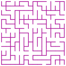
Figure 2. A random spanning tree on an $15\times 15$ square grid.

In the following, we let

(37) $${\mathsf{T}}_{\mathsf{G}}(\underline{x})=\sum_{T\in\mathcal{T}(\mathsf{G})}\underline{x}^{T}$$

be the generating polynomial of spanning trees of $\mathsf{G}$. By the classical matrix-tree theorem (31), combined with a routine calculation, summing over all choices of vertex $v_{0}$ and writing the non-zero coefficient of the characteristic polynomial of $d^{*}d$, we have

(38) $${\mathsf{T}}_{\mathsf{G}}(\underline{x})=|{\sf V}|^{-1}\det(d^{*}d)^{(\ker d)^{\perp}}_{(\ker d)^{\perp}}\,.$$

It follows from the mean projection theorem ([KL19, Theorem 5.9]) and its variant (Theorem 3.2 above), applied to the random spanning tree determinantal measure, that for any integer $k\geq 1$, we have

(39) $$\sum_{T\in\mathcal{T}(\mathsf{G})}\underline{x}^{T}\mathchoice{\raisebox{1.0pt}{$\bigwedge$}}{\raisebox{1.0pt}{$\bigwedge$}}{\raisebox{0.5pt}{$\scriptstyle\bigwedge$}}{\raisebox{0.2pt}{$\scriptscriptstyle\bigwedge$}}^{k}\mathsf{P}^{\mathop{\mathrm{im}}d}_{T}=\mathsf{T}_{\mathsf{G}}(\underline{x})\;\mathchoice{\raisebox{1.0pt}{$\bigwedge$}}{\raisebox{1.0pt}{$\bigwedge$}}{\raisebox{0.5pt}{$\scriptstyle\bigwedge$}}{\raisebox{0.2pt}{$\scriptscriptstyle\bigwedge$}}^{k}{\sf\Pi}^{\mathop{\mathrm{im}}d}$$

and

(40) $$\sum_{T\in\mathcal{T}(\mathsf{G})}\underline{x}^{T}\mathchoice{\raisebox{1.0pt}{$\bigwedge$}}{\raisebox{1.0pt}{$\bigwedge$}}{\raisebox{0.5pt}{$\scriptstyle\bigwedge$}}{\raisebox{0.2pt}{$\scriptscriptstyle\bigwedge$}}^{k}\mathsf{P}^{\ker d^{*}}_{T}=\mathsf{T}_{\mathsf{G}}(\underline{x})\;\mathchoice{\raisebox{1.0pt}{$\bigwedge$}}{\raisebox{1.0pt}{$\bigwedge$}}{\raisebox{0.5pt}{$\scriptstyle\bigwedge$}}{\raisebox{0.2pt}{$\scriptscriptstyle\bigwedge$}}^{k}{\sf\Pi}^{\ker d^{*}}\,.$$

4.3. The Symanzik case: connected spanning subgraphs

Given a subgraph $S$ of $\mathsf{G}$ with first Betti number $k\geq 0$, we denote by $\pm z_{S}\in Z_{1}(\mathsf{G},\mathbb{Z})^{\wedge k}$ the exterior product of the elements of an integral basis of $Z_{1}(S,\mathbb{Z})$. This element is defined only up to a sign.

To a subgraph $S$ of $\mathsf{G}$ with $\mathop{\rm rk}Z_{1}(S,\mathbb{Z})=k$, and an element $\vartheta\in\Omega^{1}(\mathsf{G})^{\wedge k}$, we associate the weight $|(\vartheta,z_{S})|^{2}$. A case of interest is that where $\vartheta=\theta_{1}\wedge\ldots\wedge\theta_{k}$ for some $\theta_{1},\ldots,\theta_{k}\in\Omega^{1}(\mathsf{G})$, in which case for any choice of an integral basis $(\gamma_{1},\ldots,\gamma_{k})$ of $Z_{1}(S,\mathbb{Z})$, we have

(41) $$|(\vartheta,z_{S})|^{2}=\big{|}\det\big{(}\theta_{i}(\gamma_{j})\big{)}_{1\leq i,j\leq k}\big{|}^{2}.$$

We let

(42) $${\mathsf{C}}^{(k)}_{\mathsf{G}}(\vartheta,\underline{x})=\sum_{K\in\mathcal{C}_{k}(\mathsf{G})}|(\vartheta,z_{K})|^{2}\,\underline{x}^{K}$$

be the generating polynomial of weighted connected spanning subgraphs with $k$ independent cycles.

Proposition 4.1.

Let $k\geq 1$ be an integer. Let $\vartheta$ be an element of $\Omega^{1}(\mathsf{G})^{\wedge k}$. Then

(43) $$\frac{{\mathsf{C}}^{(k)}_{\mathsf{G}}(\vartheta,\underline{x})}{{\mathsf{T}}_{\mathsf{G}}(\underline{x})}=\big{\|}\mathchoice{\raisebox{1.0pt}{$\bigwedge$}}{\raisebox{1.0pt}{$\bigwedge$}}{\raisebox{0.5pt}{$\scriptstyle\bigwedge$}}{\raisebox{0.2pt}{$\scriptscriptstyle\bigwedge$}}^{k}{\sf\Pi}^{\ker d^{*}}(\vartheta)\big{\|}^{2}.$$

Let us note that this proposition also makes sense when $k=0$.

Proof.

Let us denote by $\overline{\vartheta}$ the element of $\Omega^{1}(\mathsf{G})^{\wedge k}$ that is conjugated to $\vartheta$ with respect to the basis induced by the basis $(e^{\star})_{e\in{\sf E}^{+}}$ of $\Omega^{1}(\mathsf{G})$. Since $z_{S}$ has real (indeed integer) coefficients in the basis of $Z_{1}(\mathsf{G},\mathbb{Z})^{\wedge k}$ induced by the canonical basis ${\sf E}^{+}$ of $Z_{1}(\mathsf{G},\mathbb{Z})$, we have $(\overline{\vartheta},z_{K})=\overline{(\vartheta,z_{K})}$.

We can thus start by writing

$${\mathsf{C}}^{(k)}_{\mathsf{G}}(\vartheta,\underline{x})=\sum_{K\in\mathcal{C}_{k}(\mathsf{G})}\big{(}\overline{\vartheta}\otimes\vartheta,z_{K}\otimes z_{K}\big{)}\underline{x}^{K}=\bigg{(}\overline{\vartheta}\otimes\vartheta,\sum_{K\in\mathcal{C}_{k}(\mathsf{G})}\underline{x}^{K}z_{K}\otimes z_{K}\bigg{)}\,.$$

By Proposition 2.3 and (17), we have

$$z_{K}\otimes z_{K}=\sum_{T\in\mathcal{T}(K)}\mathchoice{\raisebox{1.0pt}{$\bigwedge$}}{\raisebox{1.0pt}{$\bigwedge$}}{\raisebox{0.5pt}{$\scriptstyle\bigwedge$}}{\raisebox{0.2pt}{$\scriptscriptstyle\bigwedge$}}^{k}{\sf Z}_{T}(e_{K\setminus T})\otimes e_{K\setminus T}=\sum_{T\in\mathcal{T}(K)}\mathchoice{\raisebox{1.0pt}{$\bigwedge$}}{\raisebox{1.0pt}{$\bigwedge$}}{\raisebox{0.5pt}{$\scriptstyle\bigwedge$}}{\raisebox{0.2pt}{$\scriptscriptstyle\bigwedge$}}^{k}({\sf J}_{\underline{x}}^{-1}\mathsf{P}^{\ker d^{*}}_{T}{\sf J}_{\underline{x}})(e_{K\setminus T})\otimes e_{K\setminus T}\,.$$

We now replace the duality pairing by evaluations of the inner product, using the equalities

$$(\vartheta,e_{K\setminus T})=(\underline{x}^{K\setminus T})^{-1}\langle\langle e^{\star}_{K\setminus T},\vartheta\rangle\rangle,$$

$$\text{and}\hskip 56.9055pt\Big{(}\overline{\vartheta},\mathchoice{\raisebox{1.0pt}{$\bigwedge$}}{\raisebox{1.0pt}{$\bigwedge$}}{\raisebox{0.5pt}{$\scriptstyle\bigwedge$}}{\raisebox{0.2pt}{$\scriptscriptstyle\bigwedge$}}^{k}({\sf J}_{\underline{x}}^{-1}\mathsf{P}^{\ker d^{*}}_{T}{\sf J}_{\underline{x}})e_{K\setminus T}\Big{)}=(\underline{x}^{K\setminus T})^{-1}\big{\langle}\big{\langle}\,\mathchoice{\raisebox{1.0pt}{$\bigwedge$}}{\raisebox{1.0pt}{$\bigwedge$}}{\raisebox{0.5pt}{$\scriptstyle\bigwedge$}}{\raisebox{0.2pt}{$\scriptscriptstyle\bigwedge$}}^{k}\mathsf{P}^{\ker d^{*}}_{T}e^{\star}_{K\setminus T},\overline{\vartheta}\,\big{\rangle}\big{\rangle}.\hskip 85.35826pt$$

Combining the previous equations, we find

$${\mathsf{C}}^{(k)}_{\mathsf{G}}(\vartheta,\underline{x})=\Big{\langle}\Big{\langle}\,\sum_{K\in\mathcal{C}_{k}(\mathsf{G})}\sum_{T\in\mathcal{T}(K)}\underline{x}^{T}(\underline{x}^{K\setminus T})^{-1}\mathchoice{\raisebox{1.0pt}{$\bigwedge$}}{\raisebox{1.0pt}{$\bigwedge$}}{\raisebox{0.5pt}{$\scriptstyle\bigwedge$}}{\raisebox{0.2pt}{$\scriptscriptstyle\bigwedge$}}^{k}\mathsf{P}^{\ker d^{*}}_{T}(e^{\star}_{K\setminus T})\otimes e^{\star}_{K\setminus T},\overline{\vartheta}\otimes\vartheta\,\Big{\rangle}\Big{\rangle}\,.$$

Exchanging sums, and relaxing a constraint which yields only additional zero coefficients, we find

$${\mathsf{C}}^{(k)}_{\mathsf{G}}(\vartheta,\underline{x}) =\Big{\langle}\Big{\langle}\,\sum_{T\in\mathcal{T}(\mathsf{G})}\sum_{F\subset{\sf E}^{+}\setminus T:|F|=k}\underline{x}^{T}(\underline{x}^{F})^{-1}\mathchoice{\raisebox{1.0pt}{$\bigwedge$}}{\raisebox{1.0pt}{$\bigwedge$}}{\raisebox{0.5pt}{$\scriptstyle\bigwedge$}}{\raisebox{0.2pt}{$\scriptscriptstyle\bigwedge$}}^{k}\mathsf{P}^{\ker d^{*}}_{T}(e^{\star}_{F})\otimes e^{\star}_{F},\overline{\vartheta}\otimes\vartheta\,\Big{\rangle}\Big{\rangle}$$

$$=\Big{\langle}\Big{\langle}\,\sum_{T\in\mathcal{T}(\mathsf{G})}\sum_{F\subset{\sf E}^{+}:|F|=k}\underline{x}^{T}(\underline{x}^{F})^{-1}\mathchoice{\raisebox{1.0pt}{$\bigwedge$}}{\raisebox{1.0pt}{$\bigwedge$}}{\raisebox{0.5pt}{$\scriptstyle\bigwedge$}}{\raisebox{0.2pt}{$\scriptscriptstyle\bigwedge$}}^{k}\mathsf{P}^{\ker d^{*}}_{T}(e^{\star}_{F})\otimes e^{\star}_{F},\overline{\vartheta}\otimes\vartheta\,\Big{\rangle}\Big{\rangle}$$

$$=\Big{\langle}\Big{\langle}\,\sum_{F\subset{\sf E}^{+}:|F|=k}(\underline{x}^{F})^{-1}\Bigg{[}\sum_{T\in\mathcal{T}(\mathsf{G})}\underline{x}^{T}\mathchoice{\raisebox{1.0pt}{$\bigwedge$}}{\raisebox{1.0pt}{$\bigwedge$}}{\raisebox{0.5pt}{$\scriptstyle\bigwedge$}}{\raisebox{0.2pt}{$\scriptscriptstyle\bigwedge$}}^{k}\mathsf{P}^{\ker d^{*}}_{T}\Bigg{]}(e^{\star}_{F})\otimes e^{\star}_{F},\overline{\vartheta}\otimes\vartheta\,\Big{\rangle}\Big{\rangle}\,.$$

We now apply the variant of the mean projection theorem (40) for the random spanning tree measure to compute the sum between the square brackets. Using also the self-adjointness of ${\sf\Pi}^{\ker d^{*}}$, and the fact that its matrix in the canonical basis of $\Omega^{1}(\mathsf{G})$ has real entries, so that it commutes to complex conjugation, we find

$${\mathsf{C}}^{(k)}_{\mathsf{G}}(\vartheta,\underline{x}) =\mathsf{T}_{\mathsf{G}}(\underline{x})\;\Big{\langle}\Big{\langle}\,\sum_{F\subset{\sf E}^{+}:|F|=k}(\underline{x}^{F})^{-1}\mathchoice{\raisebox{1.0pt}{$\bigwedge$}}{\raisebox{1.0pt}{$\bigwedge$}}{\raisebox{0.5pt}{$\scriptstyle\bigwedge$}}{\raisebox{0.2pt}{$\scriptscriptstyle\bigwedge$}}^{k}{\sf\Pi}^{\ker d^{*}}(e^{\star}_{F})\otimes e^{\star}_{F},\overline{\vartheta}\otimes\vartheta\,\Big{\rangle}\Big{\rangle}$$

$$=\mathsf{T}_{\mathsf{G}}(\underline{x})\sum_{F\subset{\sf E}^{+}:|F|=k}(\underline{x}^{F})^{-1}\big{\langle}\big{\langle}\,\mathchoice{\raisebox{1.0pt}{$\bigwedge$}}{\raisebox{1.0pt}{$\bigwedge$}}{\raisebox{0.5pt}{$\scriptstyle\bigwedge$}}{\raisebox{0.2pt}{$\scriptscriptstyle\bigwedge$}}^{k}{\sf\Pi}^{\ker d^{*}}(e^{\star}_{F}),\overline{\vartheta}\,\big{\rangle}\big{\rangle}\langle\langle e^{\star}_{F},\vartheta\rangle\rangle$$

$$=\mathsf{T}_{\mathsf{G}}(\underline{x})\sum_{F\subset{\sf E}^{+}:|F|=k}(\underline{x}^{F})^{-1}\overline{\big{\langle}\big{\langle}\,e^{\star}_{F},\mathchoice{\raisebox{1.0pt}{$\bigwedge$}}{\raisebox{1.0pt}{$\bigwedge$}}{\raisebox{0.5pt}{$\scriptstyle\bigwedge$}}{\raisebox{0.2pt}{$\scriptscriptstyle\bigwedge$}}^{k}{\sf\Pi}^{\ker d^{*}}\vartheta\,\big{\rangle}\big{\rangle}}\langle\langle e^{\star}_{F},\vartheta\rangle\rangle$$

$$=\mathsf{T}_{\mathsf{G}}(\underline{x})\;\big{\langle}\big{\langle}\,\mathchoice{\raisebox{1.0pt}{$\bigwedge$}}{\raisebox{1.0pt}{$\bigwedge$}}{\raisebox{0.5pt}{$\scriptstyle\bigwedge$}}{\raisebox{0.2pt}{$\scriptscriptstyle\bigwedge$}}^{k}{\sf\Pi}^{\ker d^{*}}\vartheta,\vartheta\,\big{\rangle}\big{\rangle}\,,$$

where for the last equality we used the fact that $\{(\underline{x}^{F})^{-1/2}e^{\star}_{F}:F\subset{\sf E}^{+},|F|=k\}$ is an orthonormal basis of $\Omega^{1}(\mathsf{G})^{\wedge k}$. ∎

Let us choose $\theta_{1},\ldots,\theta_{k}\in\Omega^{1}(\mathsf{G})$. Define the map $\omega_{\underline{\theta}}:\mathbb{C}^{k}\to\Omega^{1}(\mathsf{G},\mathbb{C})$ by $(\alpha_{1},\ldots,\alpha_{k})\mapsto\alpha_{1}\theta_{1}+\ldots+\alpha_{k}\theta_{k}$. We endow $\mathbb{C}^{k}$ with $|{\sf V}|$ times the usual inner product, where $|{\sf V}|$ is the number of vertices of our graph. On the orthogonal direct sum $\mathop{\mathrm{im}}d^{*}\oplus\mathbb{C}^{k}$, we define the linear operator $d\oplus\omega_{\underline{\theta}}$, taking its values in $\Omega^{1}(\mathsf{G})$, and we set

$$\Delta_{\underline{\theta}}=(d\oplus\omega_{\underline{\theta}})^{*}(d\oplus\omega_{\underline{\theta}})\,.$$

Proposition 4.2.

Set $\vartheta=\theta_{1}\wedge\ldots\wedge\theta_{k}$. We have

$${\mathsf{C}}^{(k)}_{\mathsf{G}}(\vartheta,\underline{x})=|{\sf V}|^{k-1}\det\Delta_{\underline{\theta}}\,.$$

For $k=0$, this proposition reduces to the classical matrix-tree theorem.

Proof.

Let us apply the Schur complement formula, under the form given by Lemma 3.4, with $E_{0}=\mathop{\mathrm{im}}d^{*}\oplus\mathbb{C}^{k}$, $E_{1}=\Omega^{1}(\mathsf{G})$, $H=\mathbb{C}^{k}$ and $u=d\oplus\omega_{\underline{\theta}}$. We find

$$\det\Delta_{\underline{\theta}}=\det(d^{*}d)^{\mathop{\mathrm{im}}d^{*}}_{\mathop{\mathrm{im}}d^{*}}\ \det\Big{(}\omega_{\underline{\theta}}^{*}{\sf\Pi}^{\ker d^{*}}\omega_{\underline{\theta}}\Big{)}.$$

The first factor is equal to $|{\sf V}|\mathsf{T}_{\mathsf{G}}(\underline{x})$ by (38). Let us compute the second. For this, let us observe that the adjoint of $\omega_{\underline{\theta}}$ is given, for all $\beta\in\Omega^{1}(\mathsf{G})$, by

$$\omega_{\underline{\theta}}^{*}(\beta)=|{\sf V}|^{-1}(\langle\langle\theta_{1},\beta\rangle\rangle,\ldots,\langle\langle\theta_{k},\beta\rangle\rangle).$$

It follows that the matrix in the canonical basis of $\mathbb{C}^{k}$ of $\omega_{\underline{\theta}}^{*}{\sf\Pi}^{\ker d^{*}}\omega_{\underline{\theta}}$ is $|{\sf V}|^{-1}\big{(}\langle\langle\theta_{i},{\sf\Pi}^{\ker d^{*}}\theta_{j}\rangle\rangle\big{)}_{1\leq i,j\leq k}$ and its determinant is

$$\det\Big{(}\omega_{\underline{\theta}}^{*}{\sf\Pi}^{\ker d^{*}}\omega_{\underline{\theta}}\Big{)}=|{\sf V}|^{-k}\big{\|}\mathchoice{\raisebox{1.0pt}{$\bigwedge$}}{\raisebox{1.0pt}{$\bigwedge$}}{\raisebox{0.5pt}{$\scriptstyle\bigwedge$}}{\raisebox{0.2pt}{$\scriptscriptstyle\bigwedge$}}^{k}{\sf\Pi}^{\ker d^{*}}\vartheta\big{\|}^{2}.$$

The sought-after identity follows directly from Proposition 4.1. ∎

Theorem 4.3.

Let $k\geq 1$ be an integer. Let $\Theta$ be a $k$-dimensional linear subspace of $\Omega^{1}(\mathsf{G})$ such that $\Theta\cap\mathop{\mathrm{im}}d=\{0\}$. Let $\vartheta$ be the exterior product of the elements of a basis of $\Theta$. The measure on $\mathcal{C}_{k}(\mathsf{G})$ which assigns to a subgraph $K$ the weight

$$\underline{x}^{K}|(\vartheta,z_{K})|^{2}$$

is not zero and the corresponding probability measure is determinantal, associated with the orthogonal projection on the subspace $\mathop{\mathrm{im}}d\oplus\Theta$.

See Figure 1 (left) for an exact sample of this measure in an example.

Proof.

Let $\theta_{1},\ldots,\theta_{k}$ be a basis of $\Theta$. The assumption that $\Theta\cap\mathop{\mathrm{im}}d=\{0\}$ implies that the operator $d\oplus\omega_{\underline{\theta}}$ has full rank $|{\sf V}|-1+k$, so that $\det\Delta_{\underline{\theta}}>0$. In particular, by Proposition 4.2, the generating polynomial of the weights considered, and hence the measure, is not zero.

By Lemma 3.1, the induced probability measure is determinantal, associated with the orthogonal projection on the range of $d\oplus\omega_{\underline{\theta}}$, that is $\mathop{\mathrm{im}}d\oplus\Theta$. ∎

It follows from Theorem 4.3 that the support of the measure (which is contained in $\mathcal{C}_{k}(\mathsf{G})$ and coincides with $\mathcal{C}_{k}(\mathsf{G})$ for a generic $\Theta$) is the set of bases of a matroid [Lyo03]. The fact that $\mathcal{C}_{k}(\mathsf{G})$ is the set of bases of a matroid is immediate from the fact that the corresponding matroid is the union of the circular matroid and the uniform matroid on $k$ elements [Oxl11].

4.4. The Kirchhoff case: acyclic spanning subgraphs (spanning forests)

Given a subgraph $S$ of $\mathsf{G}$ with $k+1\geq 1$ connected components, we denote by $\pm b_{S}\in B^{1}(\mathsf{G},\mathbb{Z})^{\wedge k}$ the exterior product of the elements of an integral basis of $B^{1}(\mathsf{G}_{/S},\mathbb{Z})$. This element is defined only up to a sign.

To a subgraph $S$ of $\mathsf{G}$ with $\mathop{\rm rk}B^{1}(\mathsf{G}_{/S},\mathbb{Z})=k$, and an element $\varphi\in\Omega_{1}(\mathsf{G})^{\wedge k}$, we associate the weight $|(\varphi,b_{S})|^{2}$. A case of interest is that where $\varphi=\phi_{1}\wedge\ldots\wedge\phi_{k}$ for some $\phi_{1},\ldots,\phi_{k}\in\Omega_{1}(\mathsf{G})$, in which case for any choice of an integral basis $(\kappa_{1},\ldots,\kappa_{k})$ of $B^{1}(\mathsf{G}_{/S},\mathbb{Z})$, we have

(44) $$|(\varphi,b_{S})|^{2}=\big{|}\det\big{(}(\phi_{i},\kappa_{j})\big{)}_{1\leq i,j\leq k}\big{|}^{2}.$$

We let

(45) $${\mathsf{A}}^{(k)}_{\mathsf{G}}(\varphi,\underline{x})=\sum_{F\in\mathcal{F}_{k+1}(\mathsf{G})}|(\varphi,b_{F})|^{2}\,\underline{x}^{F}$$

be the generating polynomial of weighted acyclic spanning subgraphs with $k$ connected components.

Proposition 4.4.

Let $k\geq 1$ be an integer. Let $\varphi$ be an element of $C_{1}(\mathsf{G},\mathbb{K})^{\wedge k}$. Then

(46) $$\frac{{\mathsf{A}}^{(k)}_{\mathsf{G}}(\varphi,\underline{x})}{{\mathsf{T}}_{\mathsf{G}}(\underline{x})}=\big{\|}\mathchoice{\raisebox{1.0pt}{$\bigwedge$}}{\raisebox{1.0pt}{$\bigwedge$}}{\raisebox{0.5pt}{$\scriptstyle\bigwedge$}}{\raisebox{0.2pt}{$\scriptscriptstyle\bigwedge$}}^{k}{\sf\Pi}^{\mathop{\mathrm{im}}d}({\sf J}_{\underline{x}}\varphi)\big{\|}^{2}.$$

Proof.

Just as in the proof of Proposition 4.1, let us denote by $\overline{\varphi}$ the element of $\Omega_{1}(\mathsf{G})^{\wedge k}$ that is conjugated to $\varphi$ with respect to the basis ${\sf E}^{+}$. Since $b_{S}$ has real (indeed integer) coefficients in the basis of $B^{1}(\mathsf{G},\mathbb{Z})^{\wedge k}$ induced by the canonical basis ${\sf E}^{+}$ of $B^{1}(\mathsf{G},\mathbb{Z})$, we have $(\overline{\varphi},b_{K})=\overline{(\varphi,b_{K})}$.

We can thus start by writing

$${\mathsf{A}}^{(k)}_{\mathsf{G}}(\varphi,\underline{x})=\sum_{F\in\mathcal{F}_{k+1}(\mathsf{G})}\big{(}\overline{\varphi}\otimes\varphi,b_{F}\otimes b_{F}\big{)}\underline{x}^{F}=\bigg{(}\overline{\varphi}\otimes\varphi,\sum_{F\in\mathcal{F}_{k+1}(\mathsf{G})}\underline{x}^{F}b_{F}\otimes b_{F}\bigg{)}\,.$$

By Proposition 2.6 and (19), we have

$$b_{F}\otimes b_{F}=\sum_{T\in\mathcal{T}(\mathsf{G}):T\supset F}\mathchoice{\raisebox{1.0pt}{$\bigwedge$}}{\raisebox{1.0pt}{$\bigwedge$}}{\raisebox{0.5pt}{$\scriptstyle\bigwedge$}}{\raisebox{0.2pt}{$\scriptscriptstyle\bigwedge$}}^{k}{\sf B}_{T}(e^{\star}_{T\setminus F})\otimes e^{\star}_{T\setminus F}=\sum_{T\in\mathcal{T}(\mathsf{G}):T\supset F}\mathchoice{\raisebox{1.0pt}{$\bigwedge$}}{\raisebox{1.0pt}{$\bigwedge$}}{\raisebox{0.5pt}{$\scriptstyle\bigwedge$}}{\raisebox{0.2pt}{$\scriptscriptstyle\bigwedge$}}^{k}\mathsf{P}^{\mathop{\mathrm{im}}d}_{T}(e^{\star}_{T\setminus F})\otimes e^{\star}_{T\setminus F}\,.$$

We now replace the duality pairing by evaluations of the inner product, using the equalities

$$(\varphi,e^{\star}_{T\setminus F})=\langle\langle{\sf J}_{\underline{x}}\varphi,e^{\star}_{K\setminus T}\rangle\rangle\quad\text{and}\quad\Big{(}\overline{\varphi},\mathchoice{\raisebox{1.0pt}{$\bigwedge$}}{\raisebox{1.0pt}{$\bigwedge$}}{\raisebox{0.5pt}{$\scriptstyle\bigwedge$}}{\raisebox{0.2pt}{$\scriptscriptstyle\bigwedge$}}^{k}\mathsf{P}^{\mathop{\mathrm{im}}d}_{T}(e^{\star}_{K\setminus T})\Big{)}=\big{\langle}\big{\langle}\,\overline{{\sf J}_{\underline{x}}\varphi},\mathchoice{\raisebox{1.0pt}{$\bigwedge$}}{\raisebox{1.0pt}{$\bigwedge$}}{\raisebox{0.5pt}{$\scriptstyle\bigwedge$}}{\raisebox{0.2pt}{$\scriptscriptstyle\bigwedge$}}^{k}\mathsf{P}^{\mathop{\mathrm{im}}d}_{T}(e^{\star}_{K\setminus T})\,\big{\rangle}\big{\rangle}\,.$$

Combining the previous equations, we find

$${\mathsf{A}}^{(k)}_{\mathsf{G}}(\varphi,\underline{x})=\Big{\langle}\Big{\langle}\,\overline{{\sf J}_{\underline{x}}\varphi}\otimes{\sf J}_{\underline{x}}\varphi,\sum_{F\in\mathcal{F}_{k+1}(\mathsf{G})}\sum_{T\in\mathcal{T}(\mathsf{G}):T\supset F}\underline{x}^{F}\mathchoice{\raisebox{1.0pt}{$\bigwedge$}}{\raisebox{1.0pt}{$\bigwedge$}}{\raisebox{0.5pt}{$\scriptstyle\bigwedge$}}{\raisebox{0.2pt}{$\scriptscriptstyle\bigwedge$}}^{k}\mathsf{P}^{\mathop{\mathrm{im}}d}_{T}(e^{\star}_{T\setminus F})\otimes e^{\star}_{T\setminus F}\,\Big{\rangle}\Big{\rangle}\,.$$

Exchanging sums, and relaxing a constraint which yields only additional zero coefficients, we find

$${\mathsf{A}}^{(k)}_{\mathsf{G}}(\varphi,\underline{x}) =\Big{\langle}\Big{\langle}\,\overline{{\sf J}_{\underline{x}}\varphi}\otimes{\sf J}_{\underline{x}}\varphi,\sum_{T\in\mathcal{T}(\mathsf{G})}\sum_{\tau\subset T:|\tau|=k}\underline{x}^{T\setminus\tau}\mathchoice{\raisebox{1.0pt}{$\bigwedge$}}{\raisebox{1.0pt}{$\bigwedge$}}{\raisebox{0.5pt}{$\scriptstyle\bigwedge$}}{\raisebox{0.2pt}{$\scriptscriptstyle\bigwedge$}}^{k}\mathsf{P}^{\mathop{\mathrm{im}}d}_{T}(e^{\star}_{\tau})\otimes e^{\star}_{\tau}\,\Big{\rangle}\Big{\rangle}$$

$$=\Big{\langle}\Big{\langle}\,\overline{{\sf J}_{\underline{x}}\varphi}\otimes{\sf J}_{\underline{x}}\varphi,\sum_{T\in\mathcal{T}(\mathsf{G})}\sum_{\tau\subset{\sf E}^{+}:|\tau|=k}\underline{x}^{T\setminus\tau}\mathchoice{\raisebox{1.0pt}{$\bigwedge$}}{\raisebox{1.0pt}{$\bigwedge$}}{\raisebox{0.5pt}{$\scriptstyle\bigwedge$}}{\raisebox{0.2pt}{$\scriptscriptstyle\bigwedge$}}^{k}\mathsf{P}^{\mathop{\mathrm{im}}d}_{T}(e^{\star}_{\tau})\otimes e^{\star}_{\tau}\,\Big{\rangle}\Big{\rangle}$$

$$=\Big{\langle}\Big{\langle}\,\overline{{\sf J}_{\underline{x}}\varphi}\otimes{\sf J}_{\underline{x}}\varphi,\sum_{\tau\subset{\sf E}^{+}:|\tau|=k}(\underline{x}^{\tau})^{-1}\Bigg{[}\sum_{T\in\mathcal{T}(\mathsf{G})}\underline{x}^{T}\mathchoice{\raisebox{1.0pt}{$\bigwedge$}}{\raisebox{1.0pt}{$\bigwedge$}}{\raisebox{0.5pt}{$\scriptstyle\bigwedge$}}{\raisebox{0.2pt}{$\scriptscriptstyle\bigwedge$}}^{k}\mathsf{P}^{\mathop{\mathrm{im}}d}_{T}\Bigg{]}(e^{\star}_{\tau})\otimes e^{\star}_{\tau}\,\Big{\rangle}\Big{\rangle}\,.$$

We now apply the mean projection theorem (39) for the random spanning tree measure to compute the sum between the square brackets. Using also the self-adjointness of ${\sf\Pi}^{\mathop{\mathrm{im}}d}$, and the fact that its matrix in the canonical basis of $\Omega^{1}(\mathsf{G})$ has real entries, so that it commutes to complex conjugation, we find

$${\mathsf{A}}^{(k)}_{\mathsf{G}}(\varphi,\underline{x}) =\mathsf{T}_{\mathsf{G}}(\underline{x})\;\Big{\langle}\Big{\langle}\,\overline{{\sf J}_{\underline{x}}\varphi}\otimes{\sf J}_{\underline{x}}\varphi,\sum_{\tau\subset{\sf E}^{+}:|\tau|=k}(\underline{x}^{\tau})^{-1}\mathchoice{\raisebox{1.0pt}{$\bigwedge$}}{\raisebox{1.0pt}{$\bigwedge$}}{\raisebox{0.5pt}{$\scriptstyle\bigwedge$}}{\raisebox{0.2pt}{$\scriptscriptstyle\bigwedge$}}^{k}{\sf\Pi}^{\mathop{\mathrm{im}}d}(e^{\star}_{\tau})\otimes e^{\star}_{\tau}\,\Big{\rangle}\Big{\rangle}$$

$$=\mathsf{T}_{\mathsf{G}}(\underline{x})\sum_{\tau\subset{\sf E}^{+}:|\tau|=k}(\underline{x}^{\tau})^{-1}\big{\langle}\big{\langle}\,\overline{{\sf J}_{\underline{x}}\varphi},\mathchoice{\raisebox{1.0pt}{$\bigwedge$}}{\raisebox{1.0pt}{$\bigwedge$}}{\raisebox{0.5pt}{$\scriptstyle\bigwedge$}}{\raisebox{0.2pt}{$\scriptscriptstyle\bigwedge$}}^{k}{\sf\Pi}^{\mathop{\mathrm{im}}d}(e^{\star}_{\tau})\,\big{\rangle}\big{\rangle}\langle\langle{\sf J}_{\underline{x}}\varphi,e^{\star}_{\tau}\rangle\rangle$$

$$=\mathsf{T}_{\mathsf{G}}(\underline{x})\sum_{\tau\subset{\sf E}^{+}:|\tau|=k}(\underline{x}^{\tau})^{-1}\overline{\langle\langle e^{\star}_{\tau},{\sf J}_{\underline{x}}\varphi\rangle\rangle}\big{\langle}\big{\langle}\,e^{\star}_{\tau},\mathchoice{\raisebox{1.0pt}{$\bigwedge$}}{\raisebox{1.0pt}{$\bigwedge$}}{\raisebox{0.5pt}{$\scriptstyle\bigwedge$}}{\raisebox{0.2pt}{$\scriptscriptstyle\bigwedge$}}^{k}{\sf\Pi}^{\mathop{\mathrm{im}}d}{\sf J}_{\underline{x}}\varphi\,\big{\rangle}\big{\rangle}$$

$$=\mathsf{T}_{\mathsf{G}}(\underline{x})\;\big{\langle}\big{\langle}\,{\sf J}_{\underline{x}}\varphi,\mathchoice{\raisebox{1.0pt}{$\bigwedge$}}{\raisebox{1.0pt}{$\bigwedge$}}{\raisebox{0.5pt}{$\scriptstyle\bigwedge$}}{\raisebox{0.2pt}{$\scriptscriptstyle\bigwedge$}}^{k}{\sf\Pi}^{\mathop{\mathrm{im}}d}{\sf J}_{\underline{x}}\varphi\,\big{\rangle}\big{\rangle}\,,$$

where for the last equality we used the fact that $\{(\underline{x}^{\tau})^{-1/2}e^{\star}_{\tau}:\tau\subset{\sf E}^{+},|\tau|=k\}$ is an orthonormal basis of $\Omega^{1}(\mathsf{G})^{\wedge k}$. ∎

Let $m:Z_{1}(\mathsf{G},\mathbb{K})\to\Omega_{1}(\mathsf{G})$ be the inclusion map.

We endow $Z_{1}(\mathsf{G},\mathbb{K})$ with the unique scalar product for which any integral basis of $Z_{1}(\mathsf{G},\mathbb{Z})$ has volume $1$. Let us choose $\phi_{1},\ldots,\phi_{k}\in\Omega^{1}(\mathsf{G})$. Define the map $\omega_{\underline{\phi}}:\mathbb{C}^{k}\to\Omega^{1}(\mathsf{G},\mathbb{C})$ by $(\alpha_{1},\ldots,\alpha_{k})\mapsto\alpha_{1}\phi_{1}+\ldots+\alpha_{k}\phi_{k}$. We endow $\mathbb{C}^{k}$ with the usual inner product. On the orthogonal direct sum $Z_{1}(\mathsf{G},\mathbb{K})\oplus\mathbb{C}^{k}$, we define the linear operator $({\sf J}_{\underline{x}}m)\oplus\omega_{\underline{\phi}}$, taking its values in $\Omega^{1}(\mathsf{G})$, and we set

$$\Box_{\underline{\phi}}=({\sf J}_{\underline{x}}(m\oplus\omega_{\underline{\phi}}))^{*}({\sf J}_{\underline{x}}(m\oplus\omega_{\underline{\phi}}))\,.$$

Proposition 4.5.

Set $\varphi=\phi_{1}\wedge\ldots\wedge\phi_{k}$. We have

$${\mathsf{A}}^{(k)}_{\mathsf{G}}(\varphi,\underline{x})=(\underline{x}^{{\sf E}^{+}})^{-1}\det\Box_{\underline{\phi}}\,.$$

Proof.

Let us apply the Schur complement formula, under the form given by Lemma 3.4, with $E_{0}=Z_{1}(\mathsf{G},\mathbb{K})\oplus\mathbb{C}^{k}$, $E_{1}=\Omega^{1}(\mathsf{G})$, $H=\mathbb{C}^{k}$ and $u=({\sf J}_{\underline{x}}m)\oplus\omega_{\underline{\phi}}$. We find

$$\det\Box_{\underline{\phi}}=\det(m^{*}({\sf J}_{\underline{x}})^{*}{\sf J}_{\underline{x}}m)\ \det\Big{(}\omega_{\underline{\phi}}^{*}({\sf J}_{\underline{x}})^{*}{\sf\Pi}^{\ker(m^{*}({\sf J}_{\underline{x}})^{*})}{\sf J}_{\underline{x}}\omega_{\underline{\phi}}\Big{)}.$$

Let $\mathscr{Z}$ be an integral basis of $Z_{1}(\mathsf{G},\mathbb{Z})$. The first factor of the right-hand side is the determinant of the Gram matrix of the images by ${\sf J}_{\underline{x}}$ of the elements of $\mathscr{Z}$. By (25), this is equal to

$$\det(m^{*}({\sf J}_{\underline{x}})^{*}{\sf J}_{\underline{x}}m)=(\underline{x}^{{\sf E}^{+}})^{-1}\mathsf{T}_{\mathsf{G}}(\underline{x}).$$

For the second, observe that

$$\ker(m^{*}({\sf J}_{\underline{x}})^{*})=\mathop{\mathrm{im}}d.$$

Let us compute the second. For this, let us observe that the adjoint of $\omega_{\underline{\phi}}$ is given, for all $\beta\in\Omega^{1}(\mathsf{G})$, by

$$\omega_{\underline{\phi}}^{*}(\beta)=(\langle\langle\phi_{1},\beta\rangle\rangle,\ldots,\langle\langle\phi_{k},\beta\rangle\rangle).$$

It follows that the matrix in the canonical basis of $\mathbb{C}^{k}$ of $\omega_{\underline{\phi}}^{*}({\sf J}_{\underline{x}})^{*}{\sf\Pi}^{\ker(m^{*}({\sf J}_{\underline{x}})^{*})}{\sf J}_{\underline{x}}\omega_{\underline{\phi}}$ is

$$\big{(}\langle\langle{\sf J}_{\underline{x}}\phi_{i},{\sf\Pi}^{\mathop{\mathrm{im}}d}{\sf J}_{\underline{x}}\phi_{j}\rangle\rangle\big{)}_{1\leq i,j\leq k},$$

and its determinant is

$$\det\Big{(}\omega_{\underline{\phi}}^{*}{\sf\Pi}^{\ker m^{*}}\omega_{\underline{\phi}}\Big{)}=\big{\|}\mathchoice{\raisebox{1.0pt}{$\bigwedge$}}{\raisebox{1.0pt}{$\bigwedge$}}{\raisebox{0.5pt}{$\scriptstyle\bigwedge$}}{\raisebox{0.2pt}{$\scriptscriptstyle\bigwedge$}}^{k}{\sf\Pi}^{\mathop{\mathrm{im}}d}({\sf J}_{\underline{x}}\varphi)\big{\|}^{2}.$$

The sought-after identity follows directly from Proposition 4.4. ∎

Theorem 4.6.

Let $k\geq 1$ be an integer. Let $\Phi$ be a $k$-dimensional linear subspace of $\Omega_{1}(\mathsf{G})$ such that $\Phi\cap Z_{1}(\mathsf{G},\mathbb{K})=\{0\}$. Let $\varphi$ be the exterior product of the elements of a basis of $\Phi$. The measure on $\mathcal{F}_{k+1}(\mathsf{G})$ which assigns to a subgraph $F$ the weight

$$\underline{x}^{F}|(\varphi,b_{F})|^{2}$$

is not zero and the corresponding probability measure is determinantal, associated with the orthogonal projection on the subspace $(\ker d^{*}\oplus{\sf J}_{\underline{x}}\Phi)^{\perp}=\mathop{\mathrm{im}}d\cap({\sf J}_{\underline{x}}\Phi)^{\perp}$.

See Figure 1 (right) for an exact sample of this measure in an example.

Proof.

Let $\phi_{1},\ldots,\phi_{k}$ be a basis of $\Phi$. The assumption that $\Phi\cap Z_{1}(\mathsf{G},\mathbb{K})=\{0\}$ implies that the operator $m\oplus\omega_{\underline{\phi}}$ has full rank, so that $\det\Box_{\underline{\phi}}>0$. In particular, by Proposition 4.5, the generating polynomial of the weights considered, and hence the measure, is not zero.

By Lemma 3.1, the induced probability measure is determinantal, associated with the orthogonal projection on the range of ${\sf J}_{\underline{x}}(m\oplus\omega_{\underline{\phi}})$, that is $(\ker d^{*}\oplus({\sf J}_{\underline{x}}\Phi))^{\perp}=\mathop{\mathrm{im}}d\cap({\sf J}_{\underline{x}}\Phi)^{\perp}$. ∎

It follows from Theorem 4.6 that the support of the measure (which is contained in $\mathcal{F}_{k+1}(\mathsf{G})$ and coincides with $\mathcal{F}_{k+1}(\mathsf{G})$ for generic $\Phi$) is the set of bases of a matroid. The fact that $\mathcal{F}_{k+1}(\mathsf{G})$ is the set of bases of a matroid is immediate from the fact that the corresponding matroid is the dual of the union of the dual of the circular matroid and the uniform matroid on $k$ elements [Oxl11].

4.5. Planar duality

Let us conclude this section by discussing the relation between connected spanning subgraphs and spanning forests in the case where $\mathsf{G}$ is the $1$-dimensional skeleton of a $2$-dimensional complex.

Let us start by assuming that $\mathsf{G}$ is a graph embedded in an oriented sphere. Let $\mathsf{G}^{\dagger}$ be the dual graph. On a set-theoretic level, the orientation of the sphere induces a bijection between the oriented edges of $\mathsf{G}$ and those of $\mathsf{G}^{\dagger}$, and we denote simply by $e^{\dagger}$ the oriented edge associated to $e$. This bijection determines two isomorphisms

$$\sharp:C_{1}(\mathsf{G},\mathbb{Z}) \longrightarrow C^{1}(\mathsf{G}^{\dagger},\mathbb{Z})\hskip 28.45274pt\text{ and } \flat:C^{1}(\mathsf{G},\mathbb{Z})\longrightarrow C_{1}(\mathsf{G}^{\dagger},\mathbb{Z})$$

$$e \longmapsto e^{\sharp}=(e^{\dagger})^{\star} e^{\star}\longmapsto(e^{\star})^{\flat}=e^{\dagger}$$

which are related by $(c^{\sharp},\alpha^{\flat})=(\alpha,c)$, for all $c\in C_{1}(\mathsf{G},\mathbb{Z})$ and $\alpha\in C^{1}(\mathsf{G},\mathbb{Z})$.

The first isomorphism sends $Z_{1}(\mathsf{G},\mathbb{Z})$ to $B^{1}(\mathsf{G}^{\dagger},\mathbb{Z})$, and the second sends $B^{1}(\mathsf{G},\mathbb{Z})$ to $Z_{1}(\mathsf{G}^{\dagger},\mathbb{Z})$. Extending the scalars to $\mathbb{K}$ yields isomorphisms from $\Omega_{1}(\mathsf{G})$ to $\Omega^{1}(\mathsf{G}^{\dagger})$, and from $\Omega^{1}(\mathsf{G})$ to $\Omega_{1}(\mathsf{G}^{\dagger})$.

Let us consider an integer $k\geq 0$ and choose $\varphi\in\Omega_{1}(\mathsf{G})^{\wedge k}$. Let us consider $\vartheta=\varphi^{\sharp}\in\Omega^{1}(\mathsf{G}^{\dagger})$ the tensor associated to $\varphi$ by the $k$-th exterior power of the first isomorphism.

Let $F\in\mathcal{F}_{k+1}(\mathsf{G})$ be a spanning forest of $\mathsf{G}$ with $k+1$ components. Then $K=(F^{c})^{\dagger}$ belongs to $\mathsf{C}_{k}(\mathsf{G}^{\dagger})$ and, with the notation of the previous sections, $z_{K}=\pm(b_{F})^{\flat}$. Then,

$$(\vartheta,z_{K})=\pm(\varphi^{\sharp},b_{F}^{\flat})=\pm(\varphi,b_{F}).$$

Let $\underline{x}$ be a set of positive weights associated with the edges of our graphs. The following proposition is then a consequence of the definitions (45) and (42) of the generating polynomials.

Proposition 4.7.

For all $\varphi\in\Omega_{1}(\mathsf{G})^{\wedge k}$, we have the equality of polynomials

(47) $$\mathsf{A}^{(k)}_{\mathsf{G}}(\varphi,\underline{x})=\underline{x}^{{\sf E}^{+}}\mathsf{C}^{(k)}_{\mathsf{G}^{\dagger}}(\varphi^{\sharp},\underline{x}^{-1})\,.$$

It follows from (47) that the determinantal measures described in Theorem 4.3 on $\mathcal{F}_{k+1}(\mathsf{G})$ and in Theorem 4.6 on $\mathcal{C}_{k}(\mathsf{G}^{\dagger})$ correspond, via the map $S\mapsto(S^{c})^{\dagger}$, up to the replacement of the subspace $\Phi$ of $\Omega_{1}(\mathsf{G})$ by the subspace $\Theta=\Phi^{\sharp}$ of $\Omega^{1}(\mathsf{G}^{\dagger})$, and of the positive weights by their inverses.

Equation (47) can also be seen as a consequence of Propositions 4.2 and 4.5, using a relation of conjugation between the operators $\Box_{\underline{\varphi}}$ on $\mathsf{G}^{\dagger}$ and $\Delta_{\underline{\theta}}$ on $\mathsf{G}$.

Incidentally, while enumerating elements in $\mathcal{F}_{k}(\mathsf{G})$ can be done in polynomial time, using a combination of determinants (see [LC81], further simplified by [Myr92] and [KW16]), we do not know if elements of $\mathcal{C}_{k}(\mathsf{G})$ can be enumerated in polynomial time. In the case where $\mathsf{G}$ is planar, this can be done by the duality discussed in this section. However, the enumerations of $\cup_{k\geq 0}\mathcal{F}_{k}(\mathsf{G})$ and $\cup_{k\geq 0}\mathcal{C}_{k}(\mathsf{G})$ are known to be impossible in polynomial time, as they are $\#P$-hard evaluations of the Tutte polynomial of $\mathsf{G}$, see [Wel93, PB83]. In particular, the uniform measure on these sets is not determinantal in general. It is nevertheless conjectured that they satisfy a form of negative dependence, see [GW04].

4.6. Two-dimensional simplicial complexes

Assume now that $\mathsf{G}=(X_{0},X_{1})$ is the $1$-skeleton of a simplicial complex $X=(X_{0},X_{1},X_{2})$ of dimension $2$. Let $d^{\prime}:\Omega^{1}(X)\to\Omega^{2}(X)$, be the coboundary map from $1$-forms to $2$-forms. Since $d^{\prime}\circ d=0$, we have $\mathop{\mathrm{im}}d\subset\ker d^{\prime}$. Let $H^{1}(X,\mathbb{Z})=\ker_{\mathbb{Z}}d^{\prime}/\mathop{\mathrm{im}}_{\mathbb{Z}}d$. Then $\dim H^{1}(X,\mathbb{Z})\otimes\mathbb{K}=b_{1}(X)$, the first Betti number of $X$.

Applying Theorem 4.3 with $\Theta=H^{1}(X,\mathbb{Z})\otimes\mathbb{K}$ (or more precisely with a supplementary subspace of $\mathop{\mathrm{im}}d$ in $\ker d^{\prime}$) yields a determinantal probability measure on $\mathcal{C}_{b_{1}(X)}(\mathsf{G})$ supported on the set $\mathcal{H}_{1}(X)$ of all $K\in\mathcal{C}_{b_{1}(X)}(\mathsf{G})$ such that the natural map $Z_{1}(K,\mathbb{Z})\to H_{1}(X,\mathbb{Z})$ is an isomorphism. In particular, $\mathcal{H}_{1}(X)$, which is the support of this measure, is the set of bases of a matroid. This case was considered by Lyons in [Lyo09, Section 3], under the name $\mathbf{P}^{1}$.

Let $\sigma_{1},\ldots,\sigma_{b_{1}(X)}$ be an integral basis of $H^{1}(X,\mathbb{Z})$ and set $\varsigma=\sigma_{1}\wedge\ldots\wedge\sigma_{b_{1}(X)}$. Then for any $K\in\mathcal{H}_{1}(X)$, we have $(\varsigma,z_{K})=\pm 1$ and our construction yields the uniform measure on $\mathcal{H}_{1}(X)$.

For example, take $X$ to be a $2$-cellulation of a closed surface $\Sigma$ of genus $g\geq 1$. Then $b_{1}(X)=2g$ and $H_{1}(X,\mathbb{Z})\simeq H_{1}(\Sigma,\mathbb{Z})\simeq\mathbb{Z}^{2g}$. Elements of the support of our measure, $\mathcal{H}_{1}(X)$, are then sometimes called $g$-quasitrees of the map $X$ in the combinatorics literature. Along with lower genera quasitrees, they appear in the definition of the Bollobás–Riordan polynomial of the cellulation [CKS11], which is known to fit in the general framework of Tutte polynomials of matroids [MS18].

Our construction can be generalized to higher dimensional complexes, following [Lyo09], see the brief discussion in Section 6.10. The above duality is then Poincaré duality $X\mapsto X^{\dagger}$ between $k$-cells and $(d-k)$-cells in a $d$-dimensional complex.

4.7. Choice of convention

Note that we could have given alternative definitions for the polynomials $\mathsf{A}_{\mathsf{G}}(\vartheta,\underline{x})$, replacing the terms $\underline{x}^{F}$ by $\underline{x}^{F^{c}}$, like in the definition of Symanzik polynomials. This would have had the advantage of simplifying certain formulas, notably those that make use of the planar duality, such as (47). However, we have chosen to endow only cochains (that is, $0$-forms and $1$-forms) with inner products (see Section 1.8) and we also prefer to define determinantal processes on the set of edges with respect to subspaces of $\Omega^{1}(\mathsf{G})$ (not of $\Omega_{1}(\mathsf{G})$), so as to compare more easily with the classical cases of the uniform spanning tree. Defining the polynomials so as they would be generating functions for these determinantal probability measures (and not their dual determinantal probability measures) was a further argument in favor of this choice. This choice will also be apparent in the way we treat with the matroid generalisation in Section 6.

5. Multivariate homogeneous real stable polynomials

In this short section, we derive a few consequences about the multivariate polynomials $\mathsf{C}^{(k)}_{\mathsf{G}}(\vartheta,\underline{x})$ and $\mathsf{A}^{(k)}_{\mathsf{G}}(\varphi,\underline{x})$, and emphasise the link with the Symanzik polynomials of theoretical physics.

5.1. Real stability

Since the multivariate polynomials $\mathsf{C}^{(k)}_{\mathsf{G}}(\vartheta,\underline{x})$ and $\mathsf{A}^{(k)}_{\mathsf{G}}(\varphi,\underline{x})$ are the generating functions of determinantal probability measures, which are strongly Rayleigh measures, these polynomials are real stable, which means that they (have real coefficients and) do not vanish when all the variables $x_{e}$ have strictly positive imaginary part, from [BBL09, Definitions 2.9–2.10, and Proposition 3.5].

Corollary 5.1.

The real multivariate polynomials $\mathsf{C}^{(k)}_{\mathsf{G}}(\vartheta,\underline{x})$ and $\mathsf{A}^{(k)}_{\mathsf{G}}(\varphi,\underline{x})$ defined in (42) and (45), respectively, are real stable.

Proof.

This is a corollary of Propositions 4.2 and 4.5 using [BBL09, Definition 2.9, 2.10, and Proposition 3.5]. ∎

Homogeneous stable polynomials as above are a special case of Lorentzian polynomials, a family of polynomials with deep connections to matroid theory [BH20].

5.2. Symanzik and Kirchhoff polynomials

Symanzik polynomials appear in Feynman integrals associated with finite graphs. We refer to the introduction of [ABBGF16] for a mathematical presentation of these integrals. Combining the (slightly modified) notations of these authors with ours, the amplitude associated with an unweighted graph $\mathsf{G}$ endowed with external momenta $\underline{\vv{q}}\in(\mathbb{R}^{D})^{\sf V}$ is the real number defined by

(48) $$I_{\mathsf{G}}(\underline{\vv{q}})=\int_{(\mathbb{R}_{+})^{{\sf E}^{+}}}\exp\left(-i\frac{\Psi^{(2)}_{\mathsf{G},\underline{\vv{q}}}(\underline{x})}{\Psi^{(1)}_{\mathsf{G}}(\underline{x})}\right)\frac{\prod_{e\in{\sf E}^{+}}dx_{e}}{\sqrt{\psi_{\mathsf{G}}(\underline{x})}}$$

where

$$\Psi^{(1)}_{\mathsf{G}}(\underline{x})=\sum_{T\in\mathcal{T}(\mathsf{G})}\underline{x}^{{\sf E}^{+}\setminus T}\quad\text{and}\quad\Psi^{(2)}_{\mathsf{G},\underline{\vv{q}}}(\underline{x})=\sum_{F=\{T,T^{\prime}\}\in\mathcal{F}_{2}(\mathsf{G})}-\langle\underline{\vv{q}}({\sf V}(T)),\underline{\vv{q}}({\sf V}(T^{\prime}))\rangle\;\underline{x}^{{\sf E}^{+}\setminus F}\,,$$

and $\langle\cdot,\cdot\rangle$ is a Minkowski bilinear form on $\mathbb{R}^{D}$. Here we used the notation

$$\underline{\vv{q}}({\sf V}(T))=\sum_{v\in{\sf V}(T)}\vv{q}(v)\in\mathbb{R}^{D}\,.$$

As already alluded to in Section 2.1.2, these polynomials are called the first and second Symanzik polynomials in the literature, see [BW10].

In physical terms, $D$ represents the dimension of space-time, so that the case $D=1$ that we will now consider seems to have little physical relevance. When $D=1$ and considering the usual norm on $\mathbb{K}$ instead of a Minkowski bilinear form, taking $q\in(\ker d)^{\perp}=\mathop{\mathrm{im}}d^{*}$ and writing it $q=d^{*}{\sf J}_{\underline{x}}\varphi$ for some $\varphi\in\Omega_{1}(\mathsf{G})$, we readily find that the second Symanzik polynomial is

(49) $$\Psi^{(2)}_{\mathsf{G},q}(\underline{x})=\sum_{F=\{T,T^{\prime}\}\in\mathcal{F}_{2}(\mathsf{G})}|q({\sf V}(T))|^{2}\,\underline{x}^{{\sf E}^{+}\setminus F}=\underline{x}^{{\sf E}^{+}}\mathsf{A}^{(1)}_{\mathsf{G}}(\varphi,\underline{x}^{-1})\,,$$

where the polynomial in the right-hand side is defined in (45).

This suggests the following generalization. Let $k\geq 2$ be an integer. Let $(\phi_{1},\ldots,\phi_{k})$ be elements of $\Omega_{1}(\mathsf{G})$ and set $q_{i}={\sf J}^{0}\partial\phi_{i}=d^{*}{\sf J}_{\underline{x}}\phi_{i}$ for all $i\in\{1\ldots,k\}$. For all $F\in\mathcal{F}_{k+1}(\mathsf{G})$ we choose $T_{1},\ldots,T_{k}$ an enumeration of the trees of $F$ except one, and consider the integral basis of $B^{1}(\mathsf{G}_{/F},\mathbb{Z})$ consisting in the set of cuts $\{\kappa_{i}=\delta(\mathbbm{1}_{{\sf V}(T_{i})}):1\leq i\leq k\}$. Thus, for all $j\in\{1,\ldots,k\}$,

$$\big{(}\kappa_{j},\phi_{i}\big{)}=\big{\langle}\big{\langle}\,{\sf J}_{\underline{x}}\phi_{i},d(\mathbbm{1}_{{\sf V}(T_{j})})\rangle\rangle=\big{\langle}\big{\langle}\,d^{*}{\sf J}_{\underline{x}}\phi_{i},\mathbbm{1}_{{\sf V}(T_{j})}\,\big{\rangle}\big{\rangle}=\sum_{v\in{\sf V}(T_{j})}q_{i}(v)$$

a quantity which we denote by $q_{i}({\sf V}(T_{j}))$. The weight of the forest $F$ given by (44) is then

$$\big{|}\det\big{(}(\phi_{i},\kappa_{j})\big{)}_{1\leq i,j\leq k}\big{|}^{2}=\big{|}\det\big{(}q_{i}({\sf V}(T_{j}))\big{)}_{1\leq i,j\leq k}\big{|}^{2}\,.$$

We may thus consider the polynomial

(50) $$\sum_{F\in\mathcal{F}_{k+1}(\mathsf{G})}\big{|}\det\big{(}q_{i}({\sf V}(T_{j}))\big{)}_{1\leq i,j\leq k}\big{|}^{2}\;\underline{x}^{{\sf E}^{+}\setminus F}\;\;\in\;\mathbb{R}[\underline{x}]$$

as a natural generalization of the second Symanzik polynomial (49) to higher order $k+1\geq 3$. This polynomial is simply $\underline{x}^{{\sf E}^{+}}\mathsf{A}^{(k)}_{\mathsf{G}}(\varphi,\underline{x}^{-1})$ defined in (45) above, where $\varphi=\phi_{1}\wedge\ldots\wedge\phi_{k}$.

Symanzik polynomials, and their ‘duals’, Kirchhoff polynomials, have also been generalized to higher order and matroids by Piquerez [Piq19], where a link to determinantal (and even hyperdeterminantal) probability measures is also briefly mentioned in the introduction. Along with the family of polynomials $\mathsf{A}^{(k)}_{\mathsf{G}}(\varphi,\underline{x})$, another natural generalization of these polynomials is the family of polynomials $\mathsf{C}_{\mathsf{G}}^{(k)}(\vartheta,\underline{x})$ defined in (42).

5.3. Ratios of Symanzik polynomials and Amini’s strong stability theorem

The first and second Symanzik polynomials are known to have interesting analytic properties. In particular, Omid Amini has shown in [Ami19, Theorem 1.1] that the ratio of the two first Symanzik polynomials, seen as a rational function of the weights $\underline{x}$, which appears in the computation of the Feynman integral (48), has bounded variation at infinity. This has applications to tropical geometry [ABBGF16].

We may rewrite this ratio of polynomials, for all $q\in\mathop{\mathrm{im}}d^{*}={\sf J}^{0}(\mathop{\mathrm{im}}\partial)$, using our notations and considering $\varphi\in\Omega_{1}(\mathsf{G})$ such that $q={\sf J}^{0}\partial\varphi$, as

(51) $$\frac{\Psi^{(2)}_{\mathsf{G},q}(\underline{x})}{\Psi^{(1)}_{\mathsf{G}}(\underline{x})}=\frac{\mathsf{A}_{\mathsf{G}}^{(1)}(\varphi,\underline{x}^{-1})}{\mathsf{T}_{\mathsf{G}}(\underline{x}^{-1})}=\big{\|}{\sf\Pi}^{\mathop{\mathrm{im}}d}({\sf J}_{\underline{y}}\varphi)\big{\|}_{\underline{y}}^{2}\,,$$

where, to prove the second equality, we used Proposition 4.4 with $k=1$ and $\underline{y}=\underline{x}^{-1}$.

Let us define the discrete Green function

$$G_{\underline{y}}=\left(\big{(}\Delta_{\underline{y}}\big{)}_{\mathop{\mathrm{im}}d^{*}}^{\mathop{\mathrm{im}}d^{*}}\right)^{-1}\in\mathrm{End}(\Omega^{0}(\mathsf{G}))$$

to be the inverse of the compression of the Laplacian $\Delta_{\underline{y}}=(d^{*}d)$ on the orthogonal of its kernel (here the adjoint it with respect to the inner product determined by $\underline{y}$). Since ${\sf\Pi}^{\mathop{\mathrm{im}}d}=dG^{-1}d^{*}$, and since $d^{*}({\sf J}_{\underline{y}}\varphi)={\sf J}^{0}\partial\varphi$ by (14), we can simplify (51) further to

(52) $$\frac{\Psi^{(2)}_{\mathsf{G},q}(\underline{x})}{\Psi^{(1)}_{\mathsf{G}}(\underline{x})}=\langle\langle q,G_{\underline{y}}q\rangle\rangle\,.$$

Note that $\Delta_{\underline{y}}f(v)=\sum_{e:\overline{e}=v}y_{e}(f(v)-f(w))$ for each $f\in\Omega^{0}(\mathsf{G})$ and vertex $v$. Moreover, since both $\mathop{\mathrm{im}}d^{*}={\sf J}^{0}\mathop{\mathrm{im}}\partial$ and the inner product on $\Omega^{0}(\mathsf{G})$ are independent of $\underline{y}=\underline{x}^{-1}$, the dependence in $\underline{x}$ of the right-hand side of (52) is only via its dependence inside $\Delta_{\underline{y}}$.

The expression (52) seems to be a discrete analog of the archimedean height-pairing considered in [ABBGF16], in view of its expression in terms of the Green function of the Riemann surface whose ‘dual graph’ (in the sense of algebraic geometry, not of graph theory) is $\mathsf{G}$ ([ABBGF16, Lemma 6.3]). This archimedean height pairing is shown in that paper to be equal to the ratio of Symanzik polynomials in a certain limit, which suggests from the above it has to do with the continuous Green function converging in that limit to the discrete Green function.

Corollary 5.2.

For all $q\in\Omega^{0}(\mathsf{G})$ such that $\sum_{v\in{\sf V}}q(v)=0$, and all set of positive weights $\underline{x}_{0}$, the rational function $F_{q}:(\mathbb{R}_{+}^{*})^{{\sf E}^{+}}\to\mathbb{R}_{+},\underline{x}\mapsto\big{\langle}\big{\langle}\,q,G_{\underline{x}^{-1}}q\,\big{\rangle}\big{\rangle}$ satisfies $F_{q}(\underline{x}+\underline{x}_{0})-F_{q}(\underline{x})=O_{\underline{x}}(1)$ as $\underline{x}\to\infty$.

Proof.

We combine (52) above and a special case of [Ami19, Theorem 1.1]. ∎

In view of the expression (52) for the ratio of polynomials in terms of the Green function, one may wonder if there is an alternative proof of (this special case of) Amini’s stability theorem based on the study of variations of the Green function when changing edge weights, and if his stability result extends to other ratios of multivariate polynomials, such as the ones appearing in Proposition 4.4 and Proposition 4.1.

6. Measured matroids

The link between matroids and determinantal probability measures on discrete sets was explicited by Lyons [Lyo03, Section 2]. The goal of this section is to generalize the content of the previous sections, which was concerned with the circular matroid and its dual, to a general linear matroid on a finite set.

In particular we wish to emphasize that both the Kirchhoff and Symanzik identities (Propositions 2.4 and 2.1) are two specializations of the same general identity for linear matroids (see Proposition 6.4 below).

For background on matroids (also known as combinatorial geometries) we refer to the textbook [Oxl11] and the short introductory paper [Ard18]. Let us recall the definition: a matroid $\mathcal{M}=(S,\mathcal{I})$ on a finite set $S$ is a non-empty collection $\mathcal{I}$ of subsets of $S$, called independent subsets, such that

• if $J\subset I$ and $I\in\mathcal{I}$, then $J\in\mathcal{I}$,

• for all $I,J\in\mathcal{I}$ with $|J|<|I|$, there exists $i\in I\setminus J$ such that $J\cup\{i\}\in\mathcal{I}$.

6.1. Linear matroids

Consider a matroid $\mathcal{M}=(S,\mathcal{I})$ on a finite (ordered) set $S$. For concreteness, we will take $S=\{1,\ldots,d\}$. We assume the matroid to be representable on $\mathbb{K}$ (see the definition just below).

6.1.1. Bases

Let $\mathcal{B}_{0}=\mathcal{B}(\mathcal{M})$ be the set of bases of $\mathcal{M}$, that is, maximal elements of $\mathcal{I}$. Let $n$ be the rank of this matroid, that is, the common cardinality of any of its bases.

For each $k\in\{0,\ldots,d-n\}$, let $\mathcal{B}_{k}=\mathcal{B}_{k}(\mathcal{M})$ be the collection of elements of $2^{S}$ of cardinality $n+k$ which contain an element of $\mathcal{B}_{0}$. Then $\mathcal{B}_{k}$ is the set of bases of a matroid denoted by $\mathcal{M}_{k}$, and that is the union of the matroid $\mathcal{M}$ and the uniform matroid of rank $k$ on $S$ [Oxl11, Section 11.3].

6.1.2. Representing map and kernel

Let $\mathbb{K}$ be $\mathbb{R}$ or $\mathbb{C}$ and let $E$ be a $d$-dimensional vector space on $\mathbb{K}$. Let $(e_{1},\ldots,e_{d})$ be a basis of $E$ indexed by $S$. To say that the matroid is representable means that there exists a linear map $\mathrm{R}$ from $E$ to some target space $F$, such that the elements of $\mathcal{I}$ are those $I\subset S$ for which the family $\{\mathrm{R}(e_{i}):i\in I\}$ is linearly independent. Thus, the subspace $Z=\ker\mathrm{R}$ encodes the linear dependence of the matroid.

Let $b$ be the dimension of $Z$. By the rank theorem in linear algebra, the rank of the matroid is thus $n=\dim\mathop{\mathrm{im}}\mathrm{R}=\dim E-\dim Z=d-b$.

For all $J\subset S$, we define $E_{J}={\mathrm{Vect}}(e_{j}:j\in J)$.

6.1.3. Restriction of a matroid

Given a subset $K$ of $S$, we define a matroid $\mathcal{M}_{K}=(K,\mathcal{I}_{K})$ on $K$ by taking the collection of its independent sets $\mathcal{I}_{K}$ to be the set of those $I\in\mathcal{I}$ which are included in $K$. This construction is called the restriction of the matroid $\mathcal{M}$ to $K$, see [Oxl11, Section 1.3].

The linear map $\mathrm{R}$ representing $\mathcal{M}$, when restricted to $E_{K}$, also linearly represents the restricted matroid $\mathcal{M}_{K}$. Its kernel is $Z_{K}=\ker\mathrm{R}\cap E_{K}$.

We will only consider the case where $K$ contains at least one basis of $\mathcal{M}$. In this case, the set of bases of $\mathcal{M}_{K}$ is $\mathcal{B}(\mathcal{M}_{K})=\{T\in\mathcal{B}_{0}:T\subset K\}$. In particular, the rank of the matroid $\mathcal{M}_{K}$ is equal to $n$, the rank of $\mathcal{M}$.

Thus, for any $k\in\{0,\ldots,d-n\}$, when $K\in\mathcal{B}_{k}$, the dimension of $Z_{K}$ is $\dim E_{K}-{\rm rk}\,\mathcal{M}_{K}=(n+k)-n=k$, again by the rank theorem of linear algebra.

6.2. Fundamental circuits and bases

Let $T\in\mathcal{B}_{0}$ be a basis of the matroid $\mathcal{M}$. For any $j\in S\setminus T$, the subset $T\cup\{j\}\notin\mathcal{I}$ is dependent, hence there is a linear combination of $\{e_{t}:t\in T\}\cup\{e_{j}\}$ which lies in $Z$. By independence of $\{\mathrm{R}(e_{t}):t\in T\}$, there is a unique such linear combination giving coefficient $1$ to $e_{j}$.

Call $\gamma(T,j)$ this uniquely defined element of $Z$. Its support, defined as those $i\in S$ for which $e_{i}$ has a non-zero coefficient in the decomposition of $\gamma(T,j)$ in the basis $(e_{i})_{i\in S}$, is, in the language of matroids, the fundamental circuit associated with $T$ and $j$, see Corollary 1.2.6 of [Oxl11] and the paragraph after it.

Lemma 6.1.

The family $\{\gamma(T,j):j\in S\setminus T\}$ is a linear basis of $Z$.

Proof.

If $j^{\prime}\neq j$ are both in the complement of $T$ in $S$, then $\gamma(T,j)$ has zero coefficient on $e_{j^{\prime}}$. This shows independence. Moreover, the family has cardinality $d-n=b=\dim Z$. ∎

We denote by $\mathscr{Z}_{T}$ the family $\{\gamma(T,j):j\in S\setminus T\}$, and call it the fundamental basis of $Z$ associated with $T$.

Let ${\sf Z}_{T}:E\to Z$ be the linear map defined by setting ${\sf Z}_{T}(e_{j})=\gamma(T,j)$ for all $j\in S\setminus T$ and ${\sf Z}_{T}(e_{i})=0$ for all $i\in T$.

Lemma 6.2.

The linear map ${\sf Z}_{T}:E\to Z$ is the projection associated to the splitting

$$E=E_{T}\oplus Z.$$

Proof.

For all $j\in S\setminus T$, we have $e_{j}-\gamma(T,j)\in E_{T}=\ker{\sf Z}_{T}$, so that ${\sf Z}_{T}(\gamma(T,j))=\gamma(T,j)$. Thus, ${\sf Z}_{T}$ is the projection on $Z$ parallel to $E_{T}$. ∎

For all $J\subset S$, let us denote by $\pi_{J}:E\to E_{J}$ the projection parallel to $E_{J^{c}}$. It follows from this lemma that

(53) $${\sf Z}_{T}\circ\pi_{T^{c}}={\rm id}_{Z}.$$

This is the analog of (7).

Let us consider $k\in\{0,\ldots,d-n\}$ and $K\in\mathcal{B}_{k}$ such that $T\subset K$.

Lemma 6.3.

The subfamily $\mathscr{Z}_{T}^{K}=\{\gamma(T,j):j\in K\setminus T\}$ of $\mathscr{Z}_{T}$ is a linear basis of $Z_{K}$.

Proof.

Since $T\subset K$, each element of $\mathscr{Z}_{T}^{K}$ belongs to $E_{K}$. The family $\mathscr{Z}_{T}^{K}$ is linearly independent as a subfamily of $\mathscr{Z}_{T}$ which is a basis of $Z$ by Lemma 6.1. Finally, the cardinality of $\mathscr{Z}_{T}^{K}$ is $k$, equal to the dimension of $Z_{K}$. ∎

6.3. The circuit-basis identity for linear matroids

The following proposition generalizes both Proposition 2.1 and Proposition 2.4. For all $J=\{i_{1}<\ldots<i_{k}\}\subset S$, we define $e_{J}=e_{i_{1}}\wedge\ldots\wedge e_{i_{k}}\in E^{\wedge k}$.

For any two bases $\mathscr{B}_{1}$ and $\mathscr{B}_{2}$ of the same space, we denote by $\det(\mathscr{B}_{1}/\mathscr{B}_{2})$ the determinant of the matrix of the vectors of $\mathscr{B}_{1}$ in $\mathscr{B}_{2}$.

Proposition 6.4 (Circuit-basis identity).

Let $\mathscr{Z}=(\gamma_{1},\ldots,\gamma_{b})$ be a basis of $Z$. Then in $E^{\wedge b}$,

(54) $$\gamma_{1}\wedge\ldots\wedge\gamma_{b}=\sum_{T\in\mathcal{B}_{0}}\det(\mathscr{Z}/\mathscr{Z}_{T})\,e_{T^{c}},$$

where $\mathscr{Z}_{T}$ is the fundamental basis of $Z$ associated with $T$.

Proof.

Let us decompose the element $\gamma_{1}\wedge\ldots\wedge\gamma_{b}$ of $E^{\wedge b}$ on the basis $\{e_{J}:|J|=b\}$:

$$\gamma_{1}\wedge\ldots\wedge\gamma_{b}=\sum_{J\subset S:|J|=b}a_{J}e_{J}.$$

Consider a subset $J$ of cardinality $b$ and assume that $S\setminus J$ is not a basis of $\mathcal{M}$. Then $E_{S\setminus J}$ intersects $Z$ in a non-trivial way. This means that there exists a non-zero linear combination $\eta=u_{1}\gamma_{1}+\ldots+u_{b}\gamma_{b}$ that belongs to $E_{S\setminus J}$. By reordering $\gamma_{1},\ldots,\gamma_{n}$ if needed, we make sure that $u_{1}\neq 0$. Then $0=(\pi_{J})^{\wedge b}(\eta\wedge\gamma_{2}\wedge\ldots\wedge\gamma_{b})=u_{1}(\pi_{J})^{\wedge b}(\gamma_{1}\wedge\ldots\wedge\gamma_{b})=u_{1}a_{J}e_{J}$, so that $a_{J}=0$.

Consider now a basis $T$ of $\mathcal{M}$. Using (53), we find

$$\gamma_{1}\wedge\ldots\wedge\gamma_{b}=({\sf Z}_{T}\circ\pi_{T^{c}})^{\wedge b}(\gamma_{1}\wedge\ldots\wedge\gamma_{b})=\sum_{J\subset S:|J|=b}a_{J}\,({\sf Z}_{T})^{\wedge b}\big{(}(\pi_{T^{c}})^{\wedge b}(e_{J})\big{)}$$

and the only non-zero term of the last sum is that corresponding to $J=T^{c}$, so that

$$\gamma_{1}\wedge\ldots\wedge\gamma_{b}=a_{T^{c}}\,({\sf Z}_{T})^{\wedge b}e_{T^{c}}.$$

The result follows from the observation that $({\sf Z}_{T})^{\wedge b}e_{T^{c}}$ is the exterior product of the elements of the basis $\mathscr{Z}_{T}$. This identifies the coefficient $a_{T^{c}}$ as $\det(\mathscr{Z}/\mathscr{Z}_{T})$ and concludes the proof. ∎

Corollary 6.5.

Let $\mathscr{Z}=(\gamma_{1},\ldots,\gamma_{b})$ be a basis of $Z$. For every basis $T$ of $\mathcal{M}$, we have, in $E^{\wedge b}$,

(55) $$\pi_{T^{c}}(\gamma_{1})\wedge\ldots\wedge\pi_{T^{c}}(\gamma_{b})=\det(\mathscr{Z}/\mathscr{Z}_{T})\,e_{T^{c}}.$$

Moreover, on $Z^{\wedge b}$,

(56) $$\sum_{T\in\mathcal{B}(\mathcal{M})}\mathchoice{\raisebox{1.0pt}{$\bigwedge$}}{\raisebox{1.0pt}{$\bigwedge$}}{\raisebox{0.5pt}{$\scriptstyle\bigwedge$}}{\raisebox{0.2pt}{$\scriptscriptstyle\bigwedge$}}^{b}\pi_{T^{c}}={\rm id}_{Z^{\wedge b}}.$$

Proof.

The first equality follows from applying $\mathchoice{\raisebox{1.0pt}{$\bigwedge$}}{\raisebox{1.0pt}{$\bigwedge$}}{\raisebox{0.5pt}{$\scriptstyle\bigwedge$}}{\raisebox{0.2pt}{$\scriptscriptstyle\bigwedge$}}^{b}\pi_{T^{c}}$ to (54) and using the fact that if $S$ and $T$ are bases of $\mathcal{M}$, then $\mathchoice{\raisebox{1.0pt}{$\bigwedge$}}{\raisebox{1.0pt}{$\bigwedge$}}{\raisebox{0.5pt}{$\scriptstyle\bigwedge$}}{\raisebox{0.2pt}{$\scriptscriptstyle\bigwedge$}}^{b}\pi_{T^{c}}(e_{S^{c}})=e_{S^{c}}$ if $S=T$ and $0$ otherwise.

The second equality follows from the first one, from (54), and the fact that $Z^{\wedge b}$ is a line generated by $\gamma_{1}\wedge\ldots\wedge\gamma_{b}$. ∎

The following proposition generalizes Proposition 2.3.

Proposition 6.6.

Let $k\in\{0,\ldots,b\}$ and $K\in\mathcal{B}_{k}$. Let $\mathscr{Z}^{K}=(\gamma_{1},\ldots,\gamma_{k})$ be a basis of $Z_{K}$. Then in $\big{(}\mathchoice{\raisebox{1.0pt}{$\bigwedge$}}{\raisebox{1.0pt}{$\bigwedge$}}{\raisebox{0.5pt}{$\scriptstyle\bigwedge$}}{\raisebox{0.2pt}{$\scriptscriptstyle\bigwedge$}}^{k}Z_{K}\big{)}^{\otimes 2}$, we have

$$\sum_{\begin{subarray}{c}T\in\mathcal{B}_{0}\\ T\subset K\end{subarray}}\det(\mathscr{Z}^{K}/\mathscr{Z}^{K}_{T})^{2}\mathchoice{\raisebox{1.0pt}{$\bigwedge$}}{\raisebox{1.0pt}{$\bigwedge$}}{\raisebox{0.5pt}{$\scriptstyle\bigwedge$}}{\raisebox{0.2pt}{$\scriptscriptstyle\bigwedge$}}^{k}{\sf Z}_{T}(e_{K\setminus T})\otimes e_{K\setminus T}=(\gamma_{1}\wedge\ldots\wedge\gamma_{k})^{\otimes 2}.$$

In more concrete terms, if for every basis $T$ of $\mathcal{M}_{K}$ we let $i_{1},\ldots,i_{k}$ be the elements of $K\setminus T$, then

$$\sum_{T\in\mathcal{B}(\mathcal{M}_{K})}\det(\mathscr{Z}^{K}/\mathscr{Z}^{K}_{T})^{2}\left(\gamma(T,i_{1})\wedge\ldots\wedge\gamma(T,i_{k})\right)\otimes\left(e_{i_{1}}\wedge\ldots\wedge e_{i_{k}}\right)=(\gamma_{1}\wedge\ldots\wedge\gamma_{k})^{\otimes 2}.$$

Proof.

Let us compute the right-hand side of the equality to prove. We apply (56) on $K$ to the second factor, and then the $k$-th exterior power of (53), also on $K$ (noting that ${\sf Z}_{T}$, when applied on $E_{K}$, acts as the projection on $Z_{K}$ parallel to $E_{T}$), to each term of the sum, to find

$$(\gamma_{1}\wedge\ldots\wedge\gamma_{k})^{\otimes 2} =\sum_{T\in\mathcal{B}(\mathcal{M}_{K})}(\gamma_{1}\wedge\ldots\wedge\gamma_{k})\otimes\mathchoice{\raisebox{1.0pt}{$\bigwedge$}}{\raisebox{1.0pt}{$\bigwedge$}}{\raisebox{0.5pt}{$\scriptstyle\bigwedge$}}{\raisebox{0.2pt}{$\scriptscriptstyle\bigwedge$}}^{k}\pi_{T^{c}}(\gamma_{1}\wedge\ldots\wedge\gamma_{k})$$

$$=\sum_{T\in\mathcal{B}(\mathcal{M}_{K})}\mathchoice{\raisebox{1.0pt}{$\bigwedge$}}{\raisebox{1.0pt}{$\bigwedge$}}{\raisebox{0.5pt}{$\scriptstyle\bigwedge$}}{\raisebox{0.2pt}{$\scriptscriptstyle\bigwedge$}}^{k}{{\sf Z}}_{T}\circ\mathchoice{\raisebox{1.0pt}{$\bigwedge$}}{\raisebox{1.0pt}{$\bigwedge$}}{\raisebox{0.5pt}{$\scriptstyle\bigwedge$}}{\raisebox{0.2pt}{$\scriptscriptstyle\bigwedge$}}^{k}\pi_{T^{c}}(\gamma_{1}\wedge\ldots\wedge\gamma_{k})\otimes\mathchoice{\raisebox{1.0pt}{$\bigwedge$}}{\raisebox{1.0pt}{$\bigwedge$}}{\raisebox{0.5pt}{$\scriptstyle\bigwedge$}}{\raisebox{0.2pt}{$\scriptscriptstyle\bigwedge$}}^{k}\pi_{T^{c}}(\gamma_{1}\wedge\ldots\wedge\gamma_{k}).$$

For each basis $T$ of $\mathcal{M}_{K}$, an application of (55) gives $\pi_{T^{c}}(\gamma_{1}\wedge\ldots\wedge\gamma_{k})=\det(\mathscr{Z}^{K}/\mathscr{Z}^{K}_{T})e_{K\setminus T}$ and the result follows. ∎

6.4. Euclidean setting and determinantal probability measure on bases

We keep considering a linear matroid $\mathcal{M}=(S,\mathcal{I})$ on $S=\{1,\ldots,d\}$, with a representation $\mathrm{R}:E\to F$, where a basis $(e_{i})_{i\in S}$ of $E$ is fixed. Let $\mathrm{D}:F^{*}\to E^{*}$ be the transposed linear map of $\mathrm{R}$, where $E^{*}$ and $F^{*}$ are the dual spaces of $E$ and $F$.

Let us endow $E^{*}$ with the dual basis $(e^{\star}_{i})_{i\in S}$ and with an inner product for which this dual basis is orthogonal. Thus, there exist a collection of positive weights $\{x_{i}:i\in S\}$ such that this scalar product is given, with a natural notation, by

(57) $$\langle\langle u,v\rangle\rangle=\sum_{i\in S}x_{i}\overline{u_{i}}v_{i}\,.$$

Let us also assume that the target space $F$ of $\mathrm{R}$ is Euclidean. Then $F^{*}$ inherits a Euclidean structure from that of $F$, and we can consider the adjoint operator $\mathrm{D}^{*}:E^{*}\to F^{*}$.

Then to each subset $T\subset S$ of cardinality $n$, we associate the subspace $E^{*}_{T}={\mathrm{Vect}}(e^{\star}_{i}:i\in T)$ and the non-negative weight

(58) $$w(T)=\det(\mathrm{D}\mathrm{D}^{*})^{E^{*}_{T}}_{E^{*}_{T}}$$

which is positive if and only if $T$ is a basis of $\mathcal{M}$. These weights thus define a measure on $\mathcal{B}_{0}$, and in this situation where the linear data representing our matroid $\mathcal{M}$ is endowed with Euclidean structures, we speak of a measured matroid.

Proposition 6.7.

The probability measure on $2^{S}$ given by normalizing (58) is supported by $\mathcal{B}_{0}$ and is the determinantal measure associated with the orthogonal projection on $\mathop{\mathrm{im}}\mathrm{D}$.

Proof.

The determinantal measure is supported by subsets of $S$ of cardinality equal to the rank of $\mathrm{D}$, that is, ${\rm codim}(\ker\mathrm{R})=n$. Let $T$ be a subset of $S$ with $|T|=n$. Let us compute the weight $w(T)$ and show that it is proportional to the probability of $T$ for the determinantal measure. Using the fact that $\mathrm{D}={\sf\Pi}^{\mathop{\mathrm{im}}\mathrm{D}}\mathrm{D}$, we have

$$\det(\mathrm{D}\mathrm{D}^{*})_{E^{*}_{T}}^{E^{*}_{T}} =\det\big{(}{\sf\Pi}^{\mathop{\mathrm{im}}\mathrm{D}}\mathrm{D}\mathrm{D}^{*}{\sf\Pi}^{\mathop{\mathrm{im}}\mathrm{D}}\big{)}_{E^{*}_{T}}^{E^{*}_{T}}$$

$$=\big{\langle}\big{\langle}\,\mathchoice{\raisebox{1.0pt}{$\bigwedge$}}{\raisebox{1.0pt}{$\bigwedge$}}{\raisebox{0.5pt}{$\scriptstyle\bigwedge$}}{\raisebox{0.2pt}{$\scriptscriptstyle\bigwedge$}}^{n}{\sf\Pi}^{\mathop{\mathrm{im}}\mathrm{D}}e^{\star}_{T},\mathchoice{\raisebox{1.0pt}{$\bigwedge$}}{\raisebox{1.0pt}{$\bigwedge$}}{\raisebox{0.5pt}{$\scriptstyle\bigwedge$}}{\raisebox{0.2pt}{$\scriptscriptstyle\bigwedge$}}^{n}(\mathrm{D}\mathrm{D}^{*})\mathchoice{\raisebox{1.0pt}{$\bigwedge$}}{\raisebox{1.0pt}{$\bigwedge$}}{\raisebox{0.5pt}{$\scriptstyle\bigwedge$}}{\raisebox{0.2pt}{$\scriptscriptstyle\bigwedge$}}^{n}{\sf\Pi}^{\mathop{\mathrm{im}}\mathrm{D}}e^{\star}_{T}\,\big{\rangle}\big{\rangle}/\|e^{\star}_{T}\|^{2}.$$

The range of $\mathchoice{\raisebox{1.0pt}{$\bigwedge$}}{\raisebox{1.0pt}{$\bigwedge$}}{\raisebox{0.5pt}{$\scriptstyle\bigwedge$}}{\raisebox{0.2pt}{$\scriptscriptstyle\bigwedge$}}^{n}{\sf\Pi}^{\mathop{\mathrm{im}}\mathrm{D}}$ is the line $(\mathop{\mathrm{im}}\mathrm{D})^{\wedge n}$, on which $\mathchoice{\raisebox{1.0pt}{$\bigwedge$}}{\raisebox{1.0pt}{$\bigwedge$}}{\raisebox{0.5pt}{$\scriptstyle\bigwedge$}}{\raisebox{0.2pt}{$\scriptscriptstyle\bigwedge$}}^{n}(\mathrm{D}\mathrm{D}^{*})$ acts by multiplication by the scalar $\det(\mathrm{D}\mathrm{D}^{*})_{\mathop{\mathrm{im}}\mathrm{D}}^{\mathop{\mathrm{im}}\mathrm{D}}$. Thus, denoting by $\iota_{\mathop{\mathrm{im}}\mathrm{D}}$ the exterior product of the elements of an orthonormal basis of $\mathop{\mathrm{im}}\mathrm{D}$,

$$w(T) =\det(\mathrm{D}\mathrm{D}^{*})_{\mathop{\mathrm{im}}\mathrm{D}}^{\mathop{\mathrm{im}}\mathrm{D}}\ \big{\|}\mathchoice{\raisebox{1.0pt}{$\bigwedge$}}{\raisebox{1.0pt}{$\bigwedge$}}{\raisebox{0.5pt}{$\scriptstyle\bigwedge$}}{\raisebox{0.2pt}{$\scriptscriptstyle\bigwedge$}}^{n}{\sf\Pi}^{\mathop{\mathrm{im}}\mathrm{D}}(e^{\star}_{T}/\|e^{\star}_{T}\|)\big{\|}^{2}$$

$$=\det(\mathrm{D}\mathrm{D}^{*})_{\mathop{\mathrm{im}}\mathrm{D}}^{\mathop{\mathrm{im}}\mathrm{D}}\ \big{|}\langle\langle\iota_{\mathop{\mathrm{im}}\mathrm{D}},e^{\star}_{T}/\|e^{\star}_{T}\|\rangle\rangle\big{|}^{2}.$$

According to the general theory of determinantal point processes (see for instance [KL19, Proposition 5.8]), the second factor is exactly the probability $\mathbb{P}({\mathsf{X}}=T)$, where ${\mathsf{X}}$ is the determinantal random subset of $S$ associated with ${\sf\Pi}^{\mathop{\mathrm{im}}\mathrm{D}}$. ∎

Note that $w(T)$ can also be written as $w(T)=\det(1^{\mathop{\mathrm{im}}\mathrm{D}^{*}}\mathrm{D}^{*}{\sf\Pi}^{E^{*}_{T}}\mathrm{D}1_{\mathop{\mathrm{im}}\mathrm{D}^{*}})$ and that under this form, the Cauchy–Binet formula gives the expression

(59) $$\sum_{T\in\mathcal{B}_{0}}w(T)=\det(\mathrm{D}^{*}\mathrm{D})^{\mathop{\mathrm{im}}\mathrm{D}^{*}}_{\mathop{\mathrm{im}}\mathrm{D}^{*}}$$

for the normalisation constant, that is also equal to $\det(\mathrm{D}\mathrm{D}^{*})_{\mathop{\mathrm{im}}\mathrm{D}}^{\mathop{\mathrm{im}}\mathrm{D}}$.

The natural pairing between $E^{*}$ and $E$ extends to exterior powers: for each $k\in\{0,\ldots,d\}$, we have, with natural notations,

(60) $$(\alpha_{1}\wedge\ldots\wedge\alpha_{k},e_{1}\wedge\ldots\wedge e_{k})=\det((\alpha_{i},e_{j}))_{1\leq i,j\leq k}\,.$$

We define the antilinear isomorphism

(61) $${\sf J}_{\underline{x}}:E\to E^{*},e_{i}\mapsto x_{i}^{-1}e_{i}^{\star}\,.$$

Thus, for all $\alpha\in E^{\star}$ and $e\in E$, we have

(62) $$(\alpha,e)=\sum_{i\in S}\alpha(e_{i})e_{i}^{\star}(e)=\langle\langle{\sf J}_{\underline{x}}e,\alpha\rangle\rangle\,.$$

More generally, we have

(63) $$(\alpha_{1}\wedge\ldots\wedge\alpha_{k},e_{1}\wedge\ldots\wedge e_{k})=\big{\langle}\big{\langle}\,{\sf J}_{\underline{x}}e_{1}\wedge\ldots\wedge{\sf J}_{\underline{x}}e_{k},\alpha_{1}\wedge\ldots\wedge\alpha_{k}\,\big{\rangle}\big{\rangle}\,.$$

The endomorphism

(64) $$\mathsf{P}_{T}={\sf J}_{\underline{x}}{\sf Z}_{T}{\sf J}_{\underline{x}}^{-1}$$

of $E^{*}$ is the projection on ${\sf J}_{\underline{x}}(Z)=\ker\mathrm{D}^{*}$ parallel to ${\sf J}_{\underline{x}}(E_{T})={\mathrm{Vect}}(e_{i}^{\star}:i\in T)=E^{*}_{T}$.

6.5. Probability density

Let ${\mathsf{X}}$ be the random determinantal subset of $S$ associated with the orthogonal projection on $\mathop{\mathrm{im}}\mathrm{D}$. This is the random subset of $S$ considered in Proposition 6.7.

Let us give an alternative expression of the probability $\mathbb{P}({\mathsf{X}}=T)$, which involves the basis $\mathscr{Z}_{T}$ of $Z$.

Proposition 6.8.

Let $\mathscr{Z}$ be a basis of $Z$. For all $T\in\mathcal{B}_{0}$, we have

$$\mathbb{P}({\mathsf{X}}=T)\propto|\det(\mathscr{Z}/\mathscr{Z}_{T})|^{2}\;\underline{x}^{T}\,.$$

Proof.

Let us write $\mathscr{Z}=(\gamma_{1},\ldots,\gamma_{b})$ and define the linear map $a:\mathbb{K}^{b}\to E^{*}$ by setting $a(r_{1},\ldots,r_{b})=r_{1}{\sf J}_{\underline{y}}\gamma_{1}+\ldots+r_{b}{\sf J}_{\underline{y}}\gamma_{b}$. Endowing $\mathbb{K}^{b}$ with the usual scalar product $\langle\cdot,\cdot\rangle$, and denoting by $(k_{1},\ldots,k_{b})$ the canonical basis, we have, for all $i,j\in\{1,\ldots,b\}$,

$$\langle k_{i},a^{*}ak_{j}\rangle=\langle\langle ak_{i},ak_{j}\rangle\rangle=\langle\langle{\sf J}_{\underline{y}}\gamma_{i},{\sf J}_{\underline{y}}\gamma_{j}\rangle\rangle_{\underline{x}},$$

so that

$$\det(a^{*}a)=\|{\sf J}_{\underline{y}}\gamma_{1}\wedge\ldots\wedge{\sf J}_{\underline{y}}\gamma_{b}\|_{\underline{x}}^{2}.$$

Applying ${\sf J}_{\underline{y}}$ and Pythagoras’ theorem to Proposition 6.4 yields

$$\det(a^{*}a)=\sum_{T\in\mathcal{B}_{0}}|\det(\mathscr{Z}/\mathscr{Z}_{T})|^{2}\,(\underline{y}^{S\setminus T})^{-2}\underline{x}^{S\setminus T}.$$

Lemma 3.1 applied to the linear map $a$, of which the range is ${\sf J}_{\underline{y}}(Z)$, implies that the determinantal measure associated with the orthogonal projection, with respect to the $\underline{x}$-weighted scalar product, on ${\sf J}_{\underline{y}}(Z)$ gives to the complement of every basis $T$ a probability proportional to $|\det(\mathscr{Z}/\mathscr{Z}_{T})|^{2}\;\,(\underline{y}^{S\setminus T})^{-2}\underline{x}^{S\setminus T}$.

Specializing this result to $\underline{y}=\underline{x}$, the determinantal measure associated with the orthogonal projection on ${\sf J}_{\underline{x}}(Z)$ gives to the complement of every basis $T$ a probability proportional to $|\det(\mathscr{Z}/\mathscr{Z}_{T})|^{2}\;\underline{x}^{T}$. The result follows from the fact that the complementary random subset of $S$ is determinantal associated with the orthogonal projection on ${\sf J}_{\underline{x}}(Z)^{\perp}=\mathop{\mathrm{im}}\mathrm{D}$ (see for instance [KL19, Proposition 4.2]). ∎

For the record, the normalizing constant is

(65) $$\sum_{T\in\mathcal{B}_{0}}|\det(\mathscr{Z}/\mathscr{Z}_{T})|^{2}\;\underline{x}^{T}=\underline{x}^{S}\|{\sf J}_{\underline{x}}\gamma_{1}\wedge\ldots\wedge{\sf J}_{\underline{x}}\gamma_{b}\|^{2}.$$

For totally unimodular matroids such as the circular matroid, the numbers $|\det(\mathscr{Z}/\mathscr{Z}_{T})|^{2}$ are independent of $T$, and the probability measure considered here turns out to be almost uniform, proportional to $\underline{x}^{T}$.

Let us express in this framework the mean projection theorem.

Corollary 6.9.

Let $\mathscr{Z}$ be a basis of $Z$. For each $k\in\{0,\ldots,b\}$, we have

(66) $$\sum_{T\in\mathcal{B}_{0}}\underline{x}^{T}|\det(\mathscr{Z}/\mathscr{Z}_{T})|^{2}\;\mathchoice{\raisebox{1.0pt}{$\bigwedge$}}{\raisebox{1.0pt}{$\bigwedge$}}{\raisebox{0.5pt}{$\scriptstyle\bigwedge$}}{\raisebox{0.2pt}{$\scriptscriptstyle\bigwedge$}}^{k}\mathsf{P}_{T}=\bigg{(}\sum_{T\in\mathcal{B}_{0}}\underline{x}^{T}|\det(\mathscr{Z}/\mathscr{Z}_{T})|^{2}\bigg{)}\;\mathchoice{\raisebox{1.0pt}{$\bigwedge$}}{\raisebox{1.0pt}{$\bigwedge$}}{\raisebox{0.5pt}{$\scriptstyle\bigwedge$}}{\raisebox{0.2pt}{$\scriptscriptstyle\bigwedge$}}^{k}{\sf\Pi}^{\ker\mathrm{D}^{*}}\,.$$

Proof.

We combine Theorem 3.2 and Proposition 6.8. ∎

6.6. Conditional probability measures

We now compute the probability density of the determinantal measure conditioned on staying inside a subset $K$ of $S$. It turns out to be the determinantal measure on the set of bases of the restricted matroid $\mathcal{M}_{K}$ (see Section 6.1.3) measured by the same linear map $\mathrm{R}$ into the Euclidean space $F$.

Proposition 6.10.

Let $K\in\mathcal{B}_{k}$. Let ${\mathsf{X}}$ be a random subset under the determinantal probability measure on $2^{S}$ associated with the orthogonal projection on $H=\mathop{\mathrm{im}}\mathrm{D}$. The determinantal random subset ${\mathsf{X}}$ of $S$ conditioned on being included in $K$ is the determinantal probability measure on $2^{K}$ associated with the orthogonal projection on ${\sf\Pi}^{E_{K}^{*}}(H)$ in $E_{K}^{*}$. Moreover,

(67) $$({\sf\Pi}^{E_{K}^{*}}(H))^{\perp}\cap E_{K}^{*}={\sf J}_{\underline{x}}Z_{K}\,,$$

and this space is the range of the transposed linear map of the restriction of $\mathrm{R}$ to $E_{K}$.

Proof.

The first assertion is a specialisation of Lemma 3.3. To prove the second equality, we observe the general identity ${\sf\Pi}^{G}(H)=G\cap(G\cap H^{\perp})^{\perp}$, that holds for any two linear subspaces of a Euclidean space, and follows from the fact for all $x\in G$ and $y\in H$, we have

$$\langle\langle x,y\rangle\rangle=\langle\langle{\sf\Pi}^{G}x,y\rangle\rangle=\langle\langle x,{\sf\Pi}^{G}y\rangle\rangle.$$

Thus, $({\sf\Pi}^{E_{K}^{*}}(H))^{\perp}\cap E_{K}^{*}=H^{\perp}\cap E_{K}^{*}=\ker\mathrm{D}^{*}\cap E_{K}^{*}={\sf J}_{\underline{x}}Z_{K}$. ∎

Corollary 6.11.

For any basis $\mathscr{Z}^{K}$ of $Z_{K}$, and all $T\in\mathcal{B}(\mathcal{M}_{K})$, we have

(68) $$\mathbb{P}\big{(}{\mathsf{X}}=T\,\big{|}\,{\mathsf{X}}\subset K\big{)}\propto\underline{x}^{T}|\det(\mathscr{Z}^{K}/\mathscr{Z}^{K}_{T})|^{2}\,.$$

Proof.

We combine Propositions 6.8 and 6.10. ∎

We use these preliminary observations to show the following property.

Lemma 6.12.

Let $\mathscr{Z}=(\eta_{1},\ldots,\eta_{b})$ be a basis of $Z$. Let $k\in\{0,\ldots,b\}$ and let $K\in\mathcal{B}_{k}$. Let $\mathscr{Z}^{K}=(\gamma_{1},\ldots,\gamma_{k})$ be a basis of $Z_{K}$. The ratio

$$\frac{|\det(\mathscr{Z}/\mathscr{Z}_{T})|^{2}}{|\det(\mathscr{Z}^{K}/\mathscr{Z}^{K}_{T})|^{2}}$$

does not depend on $T\in\mathcal{B}(\mathcal{M}_{K})$.

Proof.

In view of Proposition 6.8 and Corollary 6.11, the ratio is equal, up to a constant that may depend on $K$ but not on $T$, to

$$\frac{\mathbb{P}({\mathsf{X}}=T)}{\mathbb{P}({\mathsf{X}}=T\,|\,{\mathsf{X}}\subset K)}=\mathbb{P}({\mathsf{X}}\subset K)$$

and is thus independent of $T$. ∎

In view of Lemma 6.12, we define

(69) $$r(\mathscr{Z}:\mathscr{Z}^{K})=\frac{|\det(\mathscr{Z}/\mathscr{Z}_{T})^{2}|}{|\det(\mathscr{Z}^{K}/\mathscr{Z}_{T}^{K})^{2}|}$$

for any choice of $T\in\mathcal{B}(\mathcal{M}_{K})$. Let us record an alternative expression for this ratio, manifestly independent of $T$.

Lemma 6.13.

Let $\mathscr{Z}=(\eta_{1},\ldots,\eta_{b})$ be a basis of $Z$. Let $k\in\{0,\ldots,b\}$ and let $K\in\mathcal{B}_{k}$. Let $\mathscr{Z}^{K}=(\gamma_{1},\ldots,\gamma_{k})$ be a basis of $Z_{K}$. Then

$$r(\mathscr{Z}:\mathscr{Z}^{K})=\underline{x}^{K^{c}}\frac{\lVert({\sf J}_{\underline{x}}\pi_{K^{c}})^{\wedge b}(\eta_{1}\wedge\ldots\wedge\eta_{b})\rVert^{2}}{\lVert({\sf J}_{\underline{x}})^{\wedge k}(\gamma_{1}\wedge\ldots\wedge\gamma_{k})\rVert^{2}}\,.$$

Proof.

We use Proposition 6.4, applied to $K$ and Pythagoras’ theorem to find

$$\sum_{T^{\prime}\in\mathcal{B}(\mathcal{M}_{K})}(\underline{x}^{K\setminus T^{\prime}})^{-1}|\det(\mathscr{Z}^{K}/\mathscr{Z}^{K}_{T^{\prime}})|^{2}=\lVert{\sf J}_{\underline{x}}\gamma_{1}\wedge\ldots\wedge{\sf J}_{\underline{x}}\gamma_{k}\rVert^{2}\,.$$

Moreover, by applying Proposition 6.4 to $S$, applying $\pi_{K^{c}}$, and using Pythagora’s theorem again, we find

$$\sum_{T^{\prime}\in\mathcal{B}(\mathcal{M}_{K})}(\underline{x}^{S\setminus T^{\prime}})^{-1}|\det(\mathscr{Z}/\mathscr{Z}_{T^{\prime}})^{2}|=\lVert({\sf J}_{\underline{x}}\pi_{K^{c}})^{\wedge b}(\eta_{1}\wedge\ldots\wedge\eta_{b})\rVert^{2}\,.$$

The result follows by taking the ratio of the second equation by the first, and replacing each term $|\det(\mathscr{Z}/\mathscr{Z}_{T^{\prime}})|^{2}$ of the numerator in the left-hand side by $r(\mathscr{Z}:\mathscr{Z}^{K})|\det(\mathscr{Z}^{K}/\mathscr{Z}^{K}_{T^{\prime}})|^{2}$. ∎

Using (69), we can recast Proposition 6.6 in the following form.

Corollary 6.14.

Let $\mathscr{Z}$ be a basis of $Z$. Consider $k\in\{0,\ldots,b\}$ and $K\in\mathcal{B}_{k}$. Let $\mathscr{Z}^{K}=(\gamma_{1},\ldots,\gamma_{k})$ be a basis of $Z_{K}$. Then in $(Z^{\wedge k})^{\otimes 2}$, we have

(70) $$\sum_{\begin{subarray}{c}T\in\mathcal{B}_{0}\\ T\subset K\end{subarray}}|\det(\mathscr{Z}/\mathscr{Z}_{T})|^{2}\;\mathchoice{\raisebox{1.0pt}{$\bigwedge$}}{\raisebox{1.0pt}{$\bigwedge$}}{\raisebox{0.5pt}{$\scriptstyle\bigwedge$}}{\raisebox{0.2pt}{$\scriptscriptstyle\bigwedge$}}^{k}{{\sf Z}}_{T}(e_{K\setminus T})\otimes e_{K\setminus T}=r(\mathscr{Z}:\mathscr{Z}^{K})(\gamma_{1}\wedge\ldots\wedge\gamma_{k})^{\otimes 2}\,.$$

6.7. Dual perspectives on the measured matroid and review of the approach

In the following it will be handy to view the weights $\underline{x}$ as variables of multivariate polynomials. This will help us to prove Theorem 6.17 based on an application of Lemma 3.1.

We have seen two ways of describing the density of the determinantal probability measure associated with a measured matroid $(\mathcal{M},\mathrm{R})$ (see Propositions 6.7 and 6.8). One is based on the direct Pythagora’s approach to defining a determinantal point process from a subspace $\mathop{\mathrm{im}}\mathrm{D}$ where $\mathrm{D}$ is the transposed linear map of $\mathrm{R}$. The other corresponds to the fact that the natural circuit-basis identity (Proposition 6.4) determined by the representing map $\mathrm{R}$ gives rise to the dual probability measure on the complement of the first process (as is apparent from the expansion (54), and as we further saw in the proof of Proposition 6.8).

We use these dual perspectives below to define two natural generating polynomials: $\mathsf{B}_{\mathcal{M},\mathrm{R}}(\underline{x})$ and $\mathsf{K}_{\mathcal{M},\mathrm{R}}(\mathscr{Z},\underline{x})$. The first is somewhat more canonical than the second, since the latter also takes into argument an arbitrary basis of $Z$. The two are related by (74) so that we can play with both polynomials equally well. From the first, we establish the correspondence to the operator $\mathrm{D}$ and find a practical determinantal expression for the partition function ${\sf L}_{\mathcal{M},\mathrm{R}}^{(k)}(\mathscr{Z},\vartheta,\underline{x})$ of the determinantal measures on $\mathcal{B}_{k}$ in 6.16. Thanks to the second, we are able to use our preparatory computations, notably Corollaries 6.14 and 6.9 to prove Proposition 6.15, which computes the ratio of the polynomials ${\sf L}_{\mathcal{M},\mathrm{R}}^{(k)}(\mathscr{Z},\vartheta,\underline{x})$ and $\mathsf{K}_{\mathcal{M},\mathrm{R}}(\mathscr{Z},\underline{x})$. This result is instrumental for proving Proposition 6.16 and is of independent interest in the light of Section 5.3.

6.8. Partition functions

Let us hence define the following multivariate polynomial

(71) $$\mathsf{B}_{\mathcal{M},\mathrm{R}}(\underline{x})=\sum_{T\in\mathcal{B}_{0}}w(T)=\det(\mathrm{D}^{*}\mathrm{D})_{\mathop{\mathrm{im}}\mathrm{D}^{*}}^{\mathop{\mathrm{im}}\mathrm{D}^{*}}$$

where $w(T)$ was defined in (58), and the second equality is (59).

This is indeed a polynomial, seen as a function of $\underline{x}$. Indeed, note that $\mathrm{D}^{*}{\sf J}_{\underline{x}}={\sf J}^{0}\mathrm{R}$, where ${\sf J}^{0}:F\to F^{*}$ is the isomorphism determined by the Euclidean structure on $F$. For each $T\in\mathcal{B}_{0}$, we may rewrite the weight $w(T)$ as

$$w(T)=\det\big{(}\mathrm{D}{\sf J}^{0}\mathrm{R}({\sf J}_{\underline{x}})^{-1}\big{)}_{E^{*}_{T}}^{E^{*}_{T}}\,.$$

Writing this determinant in the canonical basis of $E^{*}_{T}$, and using the canonical basis of $E_{T}$, we see that it is a scalar multiple of $\underline{x}^{T}$, with a scalar that does not depend on $\underline{x}$.

Let us define, for each basis $\mathscr{Z}$ of $Z$, the polynomial

(72) $$\mathsf{K}_{\mathcal{M},\mathrm{R}}(\mathscr{Z},\underline{x})=\sum_{T\in\mathcal{B}_{0}}\underline{x}^{T}|\det(\mathscr{Z}/\mathscr{Z}_{T})|^{2}\,.$$

Recall that an expression of this polynomial was given in (65).

Given two bases $\mathscr{Z}$ and $\mathscr{Z}^{\prime}$ of $Z$, and for all $\underline{x}$, we have

(73) $$\mathsf{K}_{\mathcal{M},\mathrm{R}}(\mathscr{Z},\underline{x})=|\det(\mathscr{Z}/\mathscr{Z}^{\prime})|^{2}\,\mathsf{K}_{\mathcal{M},\mathrm{R}}(\mathscr{Z}^{\prime},\underline{x}).$$

By Proposition 6.7 combined with the observation made in the paragraph following (71) that $w(T)$ is a monomial proportional to $\underline{x}^{T}$, and Proposition 6.8, we can write the generating function of our determinantal probability measure on $\mathcal{B}_{0}$ in two ways as a ratio of polynomials: for all $\underline{z}$, we have

$$\mathbb{E}[\underline{z}^{T}]=\frac{\mathsf{B}_{\mathcal{M},\mathrm{R}}(\underline{x}\underline{z})}{\mathsf{B}_{\mathcal{M},\mathrm{R}}(\underline{x})}=\frac{\mathsf{K}_{\mathcal{M},\mathrm{R}}(\mathscr{Z},\underline{x}\underline{z})}{\mathsf{K}_{\mathcal{M},\mathrm{R}}(\mathscr{Z},\underline{x})}\,.$$

Taking $\underline{z}=\underline{x}^{-1}$, we thus find

(74) $$\mathsf{K}_{\mathcal{M},\mathrm{R}}(\mathscr{Z},\underline{x})\mathsf{B}_{\mathcal{M},\mathrm{R}}(\underline{1})=\mathsf{B}_{\mathcal{M},\mathrm{R}}(\underline{x})\mathsf{K}_{\mathcal{M},\mathrm{R}}(\mathscr{Z},\underline{1})\,.$$

Let $\mathscr{Z}_{0}$ be a basis of $Z$ such that

(75) $$\mathsf{B}_{\mathcal{M},\mathrm{R}}(\underline{1})=\mathsf{K}_{\mathcal{M},\mathrm{R}}(\mathscr{Z}_{0},\underline{1})\,.$$

This exists in view of (73). Then, for all $\underline{x}$, we have

(76) $$\mathsf{B}_{\mathcal{M},\mathrm{R}}(\underline{x})=\mathsf{K}_{\mathcal{M},\mathrm{R}}(\mathscr{Z}_{0},\underline{x})\,.$$

We now define the generating polynomial of weighted bases of $\mathcal{M}_{k}$. For all bases $\mathscr{Z}$ of $Z$ and all $\vartheta\in(E^{*})^{\wedge k}$, define

(77) $${\sf L}^{(k)}_{\mathcal{M},\mathrm{R}}(\mathscr{Z},\vartheta,\underline{x})=\sum_{K\in\mathcal{B}_{k}}\underline{x}^{K}\;r(\mathscr{Z}:\mathscr{Z}^{K})\;|(\vartheta,z_{K})|^{2}$$

where for each $K$, we have chosen a basis $\mathscr{Z}^{K}=(\gamma_{1},\ldots,\gamma_{k})$ of $Z_{K}$ and have defined $z_{K}=\gamma_{1}\wedge\ldots\wedge\gamma_{k}\in Z^{\wedge k}$ to be the exterior power of its elements.

In the definition of ${\sf L}^{(k)}_{\mathcal{M},\mathrm{R}}(\mathscr{Z},\vartheta,\underline{x})$, the summand indexed by $K$ does not depend on the choice of the basis $\mathscr{Z}^{K}$ of $Z_{K}$. Indeed, let ${\mathscr{W}}^{K}$ be another basis. Then $w_{K}=\det({\mathscr{W}}^{K}/\mathscr{Z}^{K})z_{K}$ and, by Lemma 6.13, $r(\mathscr{Z}:{\mathscr{W}}^{K})=|\det({\mathscr{W}}^{K}/\mathscr{Z}^{K})|^{-2}r(\mathscr{Z}:\mathscr{Z}^{k})$.

Given two bases $\mathscr{Z}$ and $\mathscr{Z}^{\prime}$ of $Z$, and for all $\underline{x}$, we have

(78) $${\sf L}^{(k)}_{\mathcal{M},\mathrm{R}}(\mathscr{Z},\vartheta,\underline{x})=|\det(\mathscr{Z}/\mathscr{Z}^{\prime})|^{2}\,{\sf L}^{(k)}_{\mathcal{M},\mathrm{R}}(\mathscr{Z}^{\prime},\vartheta,\underline{x}).$$

The following proposition generalizes Proposition 4.1.

Proposition 6.15.

For each basis $\mathscr{Z}$ of $Z$ and all $\vartheta\in(E^{*})^{\wedge k}$, we have

(79) $$\frac{{\sf L}^{(k)}_{\mathcal{M},\mathrm{R}}(\mathscr{Z},\vartheta,\underline{x})}{\mathsf{K}_{\mathcal{M},\mathrm{R}}(\mathscr{Z},\underline{x})}=\lVert\mathchoice{\raisebox{1.0pt}{$\bigwedge$}}{\raisebox{1.0pt}{$\bigwedge$}}{\raisebox{0.5pt}{$\scriptstyle\bigwedge$}}{\raisebox{0.2pt}{$\scriptscriptstyle\bigwedge$}}^{k}{\sf\Pi}^{\ker\mathrm{D}^{*}}(\vartheta)\rVert^{2}\,.$$

Proof.

First of all, for each $K\in\mathcal{B}_{k}$, we have

$$\left|(\vartheta,z_{K})\right|^{2}=\Big{(}\overline{\vartheta}\otimes\vartheta,(\gamma_{1}\wedge\ldots\wedge\gamma_{k})^{\otimes 2}\Big{)}\,.$$

By Corollary 6.14, interverting sums and removing a constraint on indices which adds only zero terms, we find

$$\sum_{K\in\mathcal{B}_{k}}\underline{x}^{K}\,r(\mathscr{Z}:\mathscr{Z}^{K})\,\left|(\vartheta,z_{K})\right|^{2} =\Big{(}\overline{\vartheta}\otimes\vartheta,\sum_{K\in\mathcal{B}_{k}}\underline{x}^{K}r(\mathscr{Z}:\mathscr{Z}^{K})\,(\gamma_{1}\wedge\ldots\wedge\gamma_{k})^{\otimes 2}\Big{)}$$

$$=\Big{(}\overline{\vartheta}\otimes\vartheta,\sum_{K\in\mathcal{B}_{k}}\underline{x}^{K}\sum_{T\in\mathcal{B}(\mathcal{M}_{K})}|\det(\mathscr{Z}/\mathscr{Z}_{T})|^{2}\mathchoice{\raisebox{1.0pt}{$\bigwedge$}}{\raisebox{1.0pt}{$\bigwedge$}}{\raisebox{0.5pt}{$\scriptstyle\bigwedge$}}{\raisebox{0.2pt}{$\scriptscriptstyle\bigwedge$}}^{k}{\sf Z}_{T}(e_{K\setminus T})\otimes e_{K\setminus T}\Big{)}$$

$$=\sum_{T\in\mathcal{B}_{0}}\Big{(}\overline{\vartheta}\otimes\vartheta,\sum_{J\subset S\setminus T:|J|=k}|\det(\mathscr{Z}/\mathscr{Z}_{T})|^{2}\underline{x}^{J}\underline{x}^{T}\mathchoice{\raisebox{1.0pt}{$\bigwedge$}}{\raisebox{1.0pt}{$\bigwedge$}}{\raisebox{0.5pt}{$\scriptstyle\bigwedge$}}{\raisebox{0.2pt}{$\scriptscriptstyle\bigwedge$}}^{k}{\sf Z}_{T}(e_{J})\otimes e_{J}\Big{)}$$

$$=\sum_{T\in\mathcal{B}_{0}}\Big{(}\overline{\vartheta}\otimes\vartheta,\sum_{J\subset S:|J|=k}|\det(\mathscr{Z}/\mathscr{Z}_{T})|^{2}\underline{x}^{J}\underline{x}^{T}\mathchoice{\raisebox{1.0pt}{$\bigwedge$}}{\raisebox{1.0pt}{$\bigwedge$}}{\raisebox{0.5pt}{$\scriptstyle\bigwedge$}}{\raisebox{0.2pt}{$\scriptscriptstyle\bigwedge$}}^{k}{\sf Z}_{T}(e_{J})\otimes e_{J}\Big{)}$$

Further, by Equation (64) and (62), and recognizing an expansion over the orthonormal basis $\{(\underline{x}^{J})^{-1/2}e_{J}^{\star}:J\subset S,|J|=k\}$ of $E^{\wedge k}$, we thus find

$${\sf L}^{(k)}_{\mathcal{M},\mathrm{R}}(\mathscr{Z},\vartheta,\underline{x}) =\sum_{J\subset S:|J|=k}(\underline{x}^{J})^{-1}\Big{\langle}\Big{\langle}\,\bigg{[}\sum_{T\in\mathcal{B}_{0}}\underline{x}^{T}|\det(\mathscr{Z}/\mathscr{Z}_{T})|^{2}\mathchoice{\raisebox{1.0pt}{$\bigwedge$}}{\raisebox{1.0pt}{$\bigwedge$}}{\raisebox{0.5pt}{$\scriptstyle\bigwedge$}}{\raisebox{0.2pt}{$\scriptscriptstyle\bigwedge$}}^{k}\mathsf{P}_{T}\bigg{]}(e^{\star}_{J})\otimes e^{\star}_{J},\overline{\vartheta}\otimes\vartheta\,\Big{\rangle}\Big{\rangle}$$

$$=\Big{\langle}\Big{\langle}\,\bigg{[}\sum_{T\in\mathcal{B}_{0}}\underline{x}^{T}|\det(\mathscr{Z}/\mathscr{Z}_{T})|^{2}\mathchoice{\raisebox{1.0pt}{$\bigwedge$}}{\raisebox{1.0pt}{$\bigwedge$}}{\raisebox{0.5pt}{$\scriptstyle\bigwedge$}}{\raisebox{0.2pt}{$\scriptscriptstyle\bigwedge$}}^{k}\mathsf{P}_{T}\bigg{]}\;\vartheta,\vartheta\,\Big{\rangle}\Big{\rangle}\,.$$

Using now the mean projection theorem, in the guise of Corollary 6.9, and noting that the coefficient for which we use antilinearity of the inner product is in fact real, we find

$$\Big{\langle}\Big{\langle}\,\bigg{[}\sum_{T\in\mathcal{B}_{0}}\underline{x}^{T}|\det(\mathscr{Z}/\mathscr{Z}_{T})|^{2}\mathchoice{\raisebox{1.0pt}{$\bigwedge$}}{\raisebox{1.0pt}{$\bigwedge$}}{\raisebox{0.5pt}{$\scriptstyle\bigwedge$}}{\raisebox{0.2pt}{$\scriptscriptstyle\bigwedge$}}^{k}\mathsf{P}_{T}\bigg{]}\;\vartheta,\vartheta\,\Big{\rangle}\Big{\rangle}=\bigg{(}\sum_{T\in\mathcal{B}_{0}}\underline{x}^{T}|\det(\mathscr{Z}/\mathscr{Z}_{T})|^{2}\bigg{)}\;\big{\langle}\big{\langle}\,\mathchoice{\raisebox{1.0pt}{$\bigwedge$}}{\raisebox{1.0pt}{$\bigwedge$}}{\raisebox{0.5pt}{$\scriptstyle\bigwedge$}}{\raisebox{0.2pt}{$\scriptscriptstyle\bigwedge$}}^{k}{\sf\Pi}^{\ker\mathrm{D}^{*}}\vartheta,\vartheta\,\big{\rangle}\big{\rangle},$$

which is equal to $\mathsf{K}_{\mathcal{M},\mathrm{R}}(\mathscr{Z},\underline{x})\;\big{\langle}\big{\langle}\,\vartheta,\mathchoice{\raisebox{1.0pt}{$\bigwedge$}}{\raisebox{1.0pt}{$\bigwedge$}}{\raisebox{0.5pt}{$\scriptstyle\bigwedge$}}{\raisebox{0.2pt}{$\scriptscriptstyle\bigwedge$}}^{k}{\sf\Pi}^{\ker\mathrm{D}^{*}}\vartheta\,\big{\rangle}\big{\rangle}$. ∎

Let us pick $\theta_{1},\ldots,\theta_{k}\in E^{*}$. Define the linear map $\omega_{\underline{\theta}}:\mathbb{K}^{k}\to E^{*},(\alpha_{1},\ldots,\alpha_{k})\mapsto\sum_{i=1}^{k}\alpha_{i}\theta_{i}$. Its adjoint is given, for all $\beta\in E^{*}$, by

$$\omega_{\underline{\theta}}^{*}(\beta)=(\langle\langle\theta_{1},\beta\rangle\rangle,\ldots,\langle\langle\theta_{k},\beta\rangle\rangle).$$

The following proposition generalizes Proposition 4.2.

Proposition 6.16.

Set $\vartheta=\theta_{1}\wedge\ldots\wedge\theta_{k}$. Let $\mathscr{Z}_{0}$ be such that (75) holds. Then

$${\sf L}^{(k)}_{\mathcal{M},\mathrm{R}}(\mathscr{Z}_{0},\vartheta,\underline{x})=\det\left((\mathrm{D}+\omega_{\underline{\theta}})^{*}(\mathrm{D}+\omega_{\underline{\theta}})\right)\,.$$

Proof.

By the Schur complement formula, in the guise of Lemma 3.4, and (71), we have

$$\det\left((\mathrm{D}+\omega_{\underline{\theta}})^{*}(\mathrm{D}+\omega_{\underline{\theta}})\right)=\det(\mathrm{D}^{*}\mathrm{D})_{\mathop{\mathrm{im}}\mathrm{D}^{*}}^{\mathop{\mathrm{im}}\mathrm{D}^{*}}\;\det\big{(}\omega_{\underline{\theta}}^{*}{\sf\Pi}^{\ker\mathrm{D}^{*}}\omega_{\underline{\theta}}\big{)}=\mathsf{B}_{\mathcal{M},\mathrm{R}}(\underline{x})\big{\|}\mathchoice{\raisebox{1.0pt}{$\bigwedge$}}{\raisebox{1.0pt}{$\bigwedge$}}{\raisebox{0.5pt}{$\scriptstyle\bigwedge$}}{\raisebox{0.2pt}{$\scriptscriptstyle\bigwedge$}}^{k}{\sf\Pi}^{\ker\mathrm{D}^{*}}\vartheta\big{\|}^{2}\,.$$

Since $\mathsf{B}_{\mathcal{M},\mathrm{R}}(\underline{x})=\mathsf{K}_{\mathcal{M},\mathrm{R}}(\mathscr{Z}_{0},\underline{x})$ by (76), the conclusion follows from Proposition 6.15. ∎

6.9. A family of determinantal probability measures

The following theorem generalizes Theorems 4.3 and 4.6. It describes a family of determinantal probability measures on the set of bases $\mathcal{B}_{k}$ of the matroid $\mathcal{M}_{k}$, with explicit weight.

Theorem 6.17.

Let $\mathscr{Z}$ be a fixed basis of $Z$. Let $k\geq 1$ and $\Theta$ be a $k$-dimensional subspace of $E^{*}$ such that $\Theta\cap\ker\mathrm{D}^{*}=\{0\}$. Let $(\theta_{1},\ldots,\theta_{k})$ be a basis of $\Theta$ and set $\vartheta=\theta_{1}\wedge\ldots\wedge\theta_{k}$. For each $K\in\mathcal{B}_{k}$, let $\mathscr{Z}^{K}=(\gamma_{1},\ldots,\gamma_{k})$ be a basis of $Z_{K}$ and set $z_{K}=\gamma_{1}\wedge\ldots\wedge\gamma_{k}$. The measure on $\mathcal{B}_{k}$ which assigns to each $K$ the weight

$$\underline{x}^{K}\,r(\mathscr{Z}:\mathscr{Z}^{K})\;|(\vartheta,z_{K})|^{2}$$

is not zero and the induced probability measure is determinantal associated with the orthogonal projection on the subspace $\mathop{\mathrm{im}}\mathrm{D}\oplus\Theta$ in the orthogonal basis $(e_{i}^{\star})_{i\in S}$.

Proof.

Under the hypothesis $\Theta\cap\ker\mathrm{D}^{*}=\{0\}$, the map $\mathrm{D}+\omega_{\underline{\theta}}$ is injective. Therefore, the determinant of $(\mathrm{D}+\omega_{\underline{\theta}})^{*}(\mathrm{D}+\omega_{\underline{\theta}})$ is positive.

Without loss of generality, we may assume that $\mathscr{Z}$ is the basis $\mathscr{Z}_{0}$ from above, satisfying (75). We now combine Proposition 6.16 and Lemma 3.1, noting that $\mathop{\mathrm{im}}(\mathrm{D}+\omega_{\underline{\theta}})$ is equal to $\mathop{\mathrm{im}}\mathrm{D}+\Theta$. ∎

6.10. Examples

In this concluding section, we record a few examples giving rise to interesting determinantal probability measures.

6.10.1. Subspaces

As is well known [Lyo03], and as we have recalled in Section 3.1 and in Section 6.4, any subspace $H$ of a finite-dimensional Euclidean $E$, coming with an orthogonal basis $(e_{i})_{i\in S}$, defines a determinantal probability measure on $S$ whose support is the set of bases of a matroid.

This probabilistic point of view implies the following interpretation of the matroid stratification of the Grassmannian of [GGMS87]. It can be understood as partitioning $\mathsf{Gr}_{n}(E)$ by assigning to each matroid $\mathcal{M}$ on $S$ of rank $n$, the set $\mathcal{G}_{\mathcal{M}}$ of subspaces $H\in\mathsf{Gr}_{n}(E)$ whose associated determinantal measure $\mathbb{P}_{H}$ in the basis $(e_{i})_{i\in S}$ has support equal to the set of bases $\mathcal{B}(\mathcal{M})$ of $\mathcal{M}$.

On the complex Grassmannian, there is a natural action of the torus $(\mathbb{C}^{*})^{d}/\mathbb{C}^{*}$ on $\mathsf{Gr}_{n}(E)$ by scaling in each direction of the basis $(e_{i})_{i\in S}$, modulo global scaling. This action is Hamiltonian with respect to the natural symplectic structure of the Grassmannian and gives rise to a moment map, which turns out to be a vectorial form of the incidence measure $\mu_{H}$, restricted to singletons, of the corresponding determinantal measure:

$$\mu:\mathsf{Gr}_{n}(E)\to\mathbb{R}^{d},\quad H\mapsto\sum_{T\in\mathcal{B}(\mathcal{M})}\mathbb{P}_{H}({\mathsf{X}}=T)\big{(}\sum_{i\in T}e_{i}\big{)}=\sum_{i=1}^{d}\mathbb{P}_{H}(i\in{\mathsf{X}})e_{i}=\sum_{i=1}^{d}\mu_{H}(\{i\})e_{i}\,.$$

Furthermore, for each matroid $\mathcal{M}$ of rank $n$, the closure of the image of $\mathcal{G}_{\mathcal{M}}$ by the moment map $\mu$ is the matroid polytope of $\mathcal{M}$, defined to be the convex hull in $\mathbb{R}^{n}$ of the collection $\{\sum_{i\in T}e_{i}:T\in\mathcal{B}(\mathcal{M})\}$, see [GGMS87, Ard21].

6.10.2. Random subgraphs

Let us stress that any subspace of $H$ of $\Omega^{1}(\mathsf{G})$, or more generally any self-dual operator $\mathsf{k}\in\mathrm{End}(\Omega^{1}(\mathsf{G}))$ satisfying $0\leq\mathsf{k}\leq 1$, gives rise to a determinantal random subgraph by means of the general theory [Lyo03].

For example, independent bond percolation, with the probability of an edge $e$ being open equal to $p_{e}$, corresponds to $\mathsf{k}(\omega_{e})=p_{e}\omega_{e}$, for $e\in{\sf E}^{+}$ (where $\omega_{e}$ was defined in Section 4.1). However some of these determinantal random subgraphs are more interesting or tractable than others. We give a few examples of interest in what follows.

It is well known that the circular and bicircular matroids of a graph are the only two matroids such that their sets of circuits are homeomorphism classes of connected graphs [SP72]. We consider now other examples of matroids on graphs.

6.10.3. Subgraphs with fixed Euler characteristic

For each $(k,\ell)\in\{0,\ldots,|{\sf V}|-1\}\times\{0,\ldots,b_{1}(\mathsf{G})\}$, there is a matroid $\mathcal{M}_{k,\ell}(\mathsf{G})$ on the set of edges of $\mathsf{G}$ whose set of bases $\mathcal{B}_{k,\ell}(\mathsf{G})$ is the collection of subgraphs $B$ of $\mathsf{G}$ satisfying

• $\chi(B)=k-\ell+1$

• $\max(0,\ell-k)\leq b_{1}(B)\leq\ell$

where $\chi(B)=b_{0}(B)-b_{1}(B)=|{\sf V}(B)|-|{\sf E}(B)|$ is the Euler characteristic of $B$. We recover the previously considered families of subgraphs: $\mathcal{B}_{0,0}(\mathsf{G})=\mathcal{T}(\mathsf{G})$, $\mathcal{B}_{0,\ell}(\mathsf{G})=\mathcal{C}_{\ell}(\mathsf{G})$ and $\mathcal{B}_{k,0}(\mathsf{G})=\mathcal{F}_{k+1}(\mathsf{G})$. The elements of $\mathcal{B}_{k,\ell}(\mathsf{G})$ are the subgraphs obtained by taking any spanning tree, adding $\ell$ edges, and then removing $k$ edges. See Figure 3.

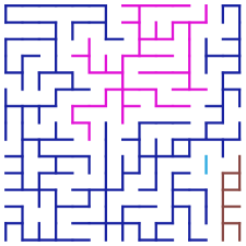
Figure 3. A determinantal random element of $\mathcal{B}_{4,4}(\mathsf{G})$ on a $15\times 15$ grid. Note that this subgraph also belongs to $\mathcal{B}_{3,3}(\mathsf{G})$, and indeed to $\mathcal{B}_{k,k}(\mathsf{G})$ for any $k\geq 3$.

The existence of these matroids, simply obtained by taking unions with the uniform matroid, or duals, starting from the circular matroid, does not contradict the result of [SP72] mentioned above. Indeed the circuits of $\mathcal{M}_{k,0}$ consist in simple cycles and spanning forests with $k$ components; because of the spanning assumption this is not the class of subgraphs homeomorphic to a fixed subclass of connected graphs. Similarly, the circuits of $\mathcal{M}_{0,\ell}(\mathsf{G})$ are the minimal subgraphs with $\ell+1$ independent cycles; because these subgraphs are not necessarily connected, this is not the class of subgraphs homeomorphic to a fixed subclass of connected graphs.

For all $(k,\ell)$ in the above range, one can define natural determinantal probability measures whose supports are included in $\mathcal{B}_{k,\ell}(\mathsf{G})$ by taking a subspace of the form $\mathop{\mathrm{im}}d\cap({\sf J}_{\underline{x}}(\Phi))^{\perp}\oplus\Theta$, with $\Phi\subset\Omega_{1}(\mathsf{G})$ a $k$-dimensional subspace such that $\Phi\cap Z_{1}(\mathsf{G},\mathbb{K})=\{0\}$ and $\Theta\subset\Omega^{1}(\mathsf{G})$ an $\ell$-dimensional subspace such that $\Theta\cap\mathop{\mathrm{im}}d\cap({\sf J}_{\underline{x}}(\Phi))^{\perp}=\{0\}$. Repeated uses of Theorem 6.17 can in principle allow us to describe explicitly these measures via geometric-topological weights on subgraphs.

6.10.4. Cycle-rooted spanning forests

The bicircular matroid of a graph $\mathsf{G}$ is the matroid on its set of unoriented edges $[{\sf E}]$, the set of bases of which is the set $\mathcal{U}(\mathsf{G})$ of cycle-rooted spanning forests. Its collection of circuits is the set of connected subgraphs with one more edge than vertices, that is the subgraphs with Betti numbers $(b_{0},b_{1})=(1,2)$. Forman [For93] proved a matrix-tree type formula for $\mathcal{U}(\mathsf{G})$ and this implies the existence of a determinantal probability measure on $\mathcal{U}(\mathsf{G})$ according to Lemma 3.1, a fact first proved by Kenyon [Ken11] who rediscovered Forman’s result, and extended it to the quaternion case. See Figure 4.

This determinantal probability measure is determined by an element $\theta\in\Omega^{1}(\mathsf{G})$, and the weight assigned to a cycle-rooted spanning forest is $\underline{x}^{F}\prod_{c\,\text{cycle}}|1-\mathrm{hol}_{h}(c)|^{2}$ where $\mathrm{hol}_{h}(c)=e^{i\theta(c)}$ is the holonomy of the cycle $c$. The corresponding subspace of $\Omega^{1}(\mathsf{G})$ is the range of a discrete covariant derivative $d_{h}$, a twisted analog of the coboundary operator $d$, where $h$ is a connection which represents $\theta$ in the sense that $h_{e}=\exp(i\theta_{e})$ (for detailed definitions, see [Ken11, Kas15, KL19, KL22b]).

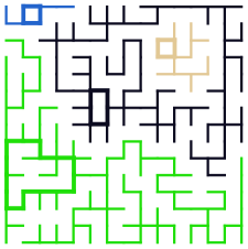
Figure 4. A determinantal random cycle-rooted spanning forest, that is a random basis of the bicircular matroid of a $15\times 15$ grid. Its cycles are represented by thickened edges. Note incidentally that this subgraph also belongs to $\mathcal{B}_{3,4}$.

As in the circular case above, we may define, for all $(k,\ell)\in\{0,\ldots,|{\sf V}|\}\times\{0,\ldots,b_{1}(\mathsf{G})-1\}$, variants $\mathcal{M}^{\text{bicirc}}_{k,l}(\mathsf{G})$, where $\mathcal{M}^{\text{bicirc}}_{0,0}(\mathsf{G})$ is the bicircular matroid of $\mathsf{G}$. The collection of bases of $\mathcal{M}^{\text{bicirc}}_{k,l}(\mathsf{G})$ is obtained as the collection of subgraphs of $\mathsf{G}$ built by adding $k$ edges to any element of $\mathcal{U}(\mathsf{G})$, and then removing $\ell$ edges.

For all $(k,\ell)$ in the above range, we can define natural determinantal probability measures whose support is included in $\mathcal{B}_{k,\ell}^{\text{bicirc}}(\mathsf{G})$, by considering a subspace of the form $\mathop{\mathrm{im}}d_{h}\cap({\sf J}_{\underline{x}}(\Phi))^{\perp}\oplus\Theta$ with assumptions similar to those in the circular case. The description of weights can in principle be obtained using Theorem 6.17 but we have not worked this out.

As proved by Kenyon in [Ken11, Theorem 3], when we consider $\varepsilon\theta$ in place of $\theta$, then, letting $\varepsilon$ tend to $0$, we have a family of determinantal measures on $\mathcal{U}(\mathsf{G})$ converging to a determinantal measure on $\mathcal{C}_{1}(\mathsf{G})$, which is precisely the measure described in Theorem 4.3 for the line $\Theta=\mathbb{K}\theta$. We generalize this convergence result to higher rank in [KL22b].

Incidentally, let us record the following interesting fact. Finding the number of elements of $\mathcal{U}(\mathsf{G})$ is known to be $\#P$-hard [GN06, Section 3], and thus there can be no polynomial time computable formula for it. In particular, the uniform measure on $\mathcal{U}(\mathsf{G})$ cannot be determinantal, by Lemma 3.1, or by [Lyo03, Corollary 5.5]. However, the uniform measure on $\mathcal{U}(\mathsf{G})$ may be sampled exactly in polynomial time, see [KK17, Theorem 1], [Kas15, Section 2.4], and [GJ21]. This yields a fully-polynomial approximation scheme (FPRAS) for enumerating $\mathcal{U}(\mathsf{G})$, as shown in [GJ21].

Further note, that the bicircular is not unimodular (otherwise there would be a determinantal expression for its number of bases [Mau76]), hence it is not regular [Whi87, Theorem 3.1.1], and hence, by a theorem of Tutte, it is not representable both on $\mathbb{F}_{2}$ and $\mathbb{F}_{3}$. However as any transversal matroid, bicircular matroids are representable over any infinite field. The question of finding over which finite fields they are representable has been studied partially by Zaslavsky.

6.10.5. Quantum spanning forests

In [KL19, Section 1.5] and [KL22b], we consider higher rank vector bundles on graphs, following our work [KL21]. We consider a subspace $\mathop{\mathrm{im}}d_{h}$ of $\Omega^{1}(\mathsf{G},\mathbb{K}^{N})$ where $d_{h}$ is a $\mathsf{U}(N,\mathbb{K})$-twisted discrete covariant derivative. Here, $\mathsf{U}(N,\mathbb{K})$ is the unitary group of $\mathbb{K}^{N}$. The quantum spanning forest is the determinantal linear process [KL19, Definition 3.1] associated with the subspace $\mathop{\mathrm{im}}d_{h}$ and the natural splitting of $\Omega^{1}(\mathsf{G},\mathbb{K}^{N})$ as sums of blocks $\mathbb{K}^{N}$, where the sum is over ${\sf E}^{+}$. It is a certain random subspace ${\mathsf{Q}}$ of the form ${\mathsf{Q}}=\oplus_{e\in{\sf E}^{+}}{\mathsf{Q}}_{e}$ which is $h$-acyclic in the sense that ${\mathsf{Q}}\cap\ker d_{h}^{*}=\{0\}$ and which is maximal for these properties.

Viewing $\Omega^{1}(\mathsf{G})$ as a linear subspace of $\Omega^{1}(\mathsf{G},\mathbb{K}^{N})$ by picking a line over each edge, we then consider the compression on that subspace of the orthogonal projection onto $\mathop{\mathrm{im}}d_{h}$. It is an element of $\mathrm{End}(\Omega^{1}(\mathsf{G}))$, which defines a determinantal random subgraph, which we call a marginal of the quantum spanning forest. See Figure 5. If we take a full orthogonal basis of each block $\mathbb{K}^{N}$ over each edge, we then obtain a collection of $N$ correlated marginal subgraphs, which are the marginals of the quantum spanning forest.

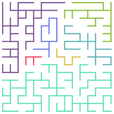
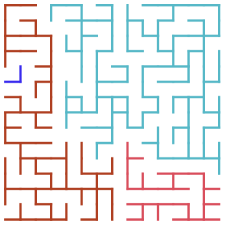
Figure 5. The marginals of a rank-$2$ quantum spanning forest on a $15\times 15$ grid.

By [KL19, Proposition 6.13], in the case where holonomies of loops are in $\mathrm{SU}(2)$, the law of the total occupation number of the marginals of the quantum spanning forest (like those in Figure 5) is equal to the occupation number of the union of two independent samples of the associated Q-determinantal measure on $\mathcal{U}(\mathsf{G})$ (like that in Figure 4).

6.10.6. Higher dimensional random simplicial complexes

Instead of the circular or bicircular matroids and their variants on graphs, one can consider matroids on the cells of higher dimensional simplicial complexes such as the ones defined in [Lyo09] (see also [Kal83, CCK15, DKM15]), which could be called ‘circular’ or ‘co-circular’, and those mentioned in [KL19, Section 1.5] which are associated to twisted coboundary maps, and could be called ‘bicircular’. The corresponding partition functions would generalize the Kirchhoff and Symanzik polynomials, and might be related to those of [Piq19].

References

- [ABBGF16] O. Amini, S. Bloch, J. I. Burgos Gil, and J. Fresán. Feynman amplitudes and limits of heights. Izv. Ross. Akad. Nauk Ser. Mat., 80(5):5–40, 2016. MR3588803
- [ABKS14] Y. An, M. Baker, G. Kuperberg, and F. Shokrieh. Canonical representatives for divisor classes on tropical curves and the matrix-tree theorem. Forum Math. Sigma, 2:Paper No. e24, 25, 2014. MR3264262
- [Ald90] D. J. Aldous. The random walk construction of uniform spanning trees and uniform labelled trees. SIAM J. Discrete Math., 3(4):450–465, 1990. MR1069105
- [Ami19] O. Amini. The exchange graph and variations of the ratio of the two Symanzik polynomials. Ann. Inst. Henri Poincaré D, 6(2):155–197, 2019. MR3950652
- [Ard18] F. Ardila. The geometry of matroids. Notices Amer. Math. Soc., 65(8):902–908, 2018. MR3823027
- [Ard21] F. Ardila. The geometry of geometries: matroid theory, old and new. ICM 2022 proceedings (submitted), 2021. arXiv:2111.08726.
- [BBGJ07] J. Bouttier, M. Bowick, E. Guitter, and M. Jeng. Vacancy localization in the square dimer model. Phys. Rev. E, 76:041140, Oct 2007.
- [BBL09] J. Borcea, P. Brändén, and T. M. Liggett. Negative dependence and the geometry of polynomials. J. Amer. Math. Soc., 22(2):521–567, 2009. MR2476782
- [BdlHN97] R. Bacher, P. de la Harpe, and T. Nagnibeda. The lattice of integral flows and the lattice of integral cuts on a finite graph. Bull. Soc. Math. France, 125(2):167–198, 1997. MR1478029
- [BH20] P. Brändén and J. Huh. Lorentzian polynomials. Ann. of Math. (2), 192(3):821–891, 2020. MR4172622
- [Big74] N. Biggs. Algebraic graph theory. Cambridge Univ. Press, 1974. Cambridge Tracts in Mathematics, No. 67. MR0347649
- [Big97] N. Biggs. Algebraic potential theory on graphs. Bull. London Math. Soc., 29(6):641–682, 1997. MR1468054
- [Big99] N. L. Biggs. Chip-firing and the critical group of a graph. J. Algebraic Combin., 9(1):25–45, 1999. MR1676732
- [BLPS01] I. Benjamini, R. Lyons, Y. Peres, and O. Schramm. Uniform spanning forests. Ann. Probab., 29(1):1–65, 2001. MR1825141
- [Bor11] A. Borodin. Determinantal point processes. In The Oxford handbook of random matrix theory, pages 231–249. Oxford Univ. Press, Oxford, 2011. MR2932631
- [BP93] R. Burton and R. Pemantle. Local characteristics, entropy and limit theorems for spanning trees and domino tilings via transfer-impedances. Ann. Probab., 21(3):1329–1371, 1993. MR1235419
- [BW10] C. Bogner and S. Weinzierl. Feynman graph polynomials. Internat. J. Modern Phys. A, 25(13):2585–2618, 2010. MR2651267
- [CCK13] M. J. Catanzaro, V. Y. Chernyak, and J. R. Klein. On Kirchhoff’s theorems with coefficients in a line bundle. Homology Homotopy Appl., 15(2):267–280, 2013. MR3138380
- [CCK15] M. J. Catanzaro, V. Y. Chernyak, and J. R. Klein. Kirchhoff’s theorems in higher dimensions and Reidemeister torsion. Homology Homotopy Appl., 17(1):165–189, 2015. MR3338546
- [CKS11] A. Champanerkar, I. Kofman, and N. Stoltzfus. Quasi-tree expansion for the Bollobás-Riordan-Tutte polynomial. Bull. Lond. Math. Soc., 43(5):972–984, 2011. MR2854567
- [CP18] S. Corry and D. Perkinson. Divisors and sandpiles. American Mathematical Society, Providence, RI, 2018. An introduction to chip-firing. MR3793659
- [DKM15] A. M. Duval, C. J. Klivans, and J. L. Martin. Cuts and flows of cell complexes. J. Algebraic Combin., 41(4):969–999, 2015. MR3342708
- [For93] R. Forman. Determinants of Laplacians on graphs. Topology, 32(1):35–46, 1993. MR1204404
- [GdMN05] O. Giménez, A. de Mier, and M. Noy. On the number of bases of bicircular matroids. Ann. Comb., 9(1):35–45, 2005. MR2135774
- [GGMS87] I. M. Gel’fand, R. M. Goresky, R. D. MacPherson, and V. V. Serganova. Combinatorial geometries, convex polyhedra, and Schubert cells. Adv. in Math., 63(3):301–316, 1987. MR877789
- [GJ21] H. Guo and M. Jerrum. Approximately counting bases of bicircular matroids. Combin. Probab. Comput., 30(1):124–135, 2021. MR4205662
- [GN06] O. Giménez and M. Noy. On the complexity of computing the Tutte polynomial of bicircular matroids. Combin. Probab. Comput., 15(3):385–395, 2006. MR2216475
- [GP14] I. Gorodezky and I. Pak. Generalized loop-erased random walks and approximate reachability. Random Structures & Algorithms, 44(2):201–223, 2014.
- [GW04] G. R. Grimmett and S. N. Winkler. Negative association in uniform forests and connected graphs. Random Structures & Algorithms, 24(4):444–460, 2004. MR2060630
- [HKPV06] J. B. Hough, M. Krishnapur, Y. Peres, and B. Virág. Determinantal processes and independence. Probab. Surv., 3:206–229, 2006. MR2216966
- [Jer21] M. Jerrum. Fundamentals of Partial Rejection Sampling. 2021. arXiv:2106.07744.
- [Kal83] G. Kalai. Enumeration of -acyclic simplicial complexes. Israel J. Math., 45(4):337–351, 1983. MR720308
- [Kas15] A. Kassel. Learning about critical phenomena from scribbles and sandpiles. In Modélisation Aléatoire et Statistique—Journées MAS 2014, volume 51 of ESAIM Proc. Surveys, pages 60–73. EDP Sci., Les Ulis, 2015. MR3440791
- [Ken11] R. Kenyon. Spanning forests and the vector bundle Laplacian. Ann. Probab., 39(5):1983–2017, 2011. MR2884879
- [Kir47] G. Kirchhoff. Ueber die Auflösung der Gleichungen, auf welche man bei der Untersuchung der linearen Vertheilung galvanischer Ströme geführt wird. Ann. Phys. und Chem., 72(12):497–508, 1847.
- [KK17] A. Kassel and R. Kenyon. Random curves on surfaces induced from the Laplacian determinant. Ann. Probab., 45(2):932–964, 2017. MR3630290
- [KL19] A. Kassel and T. Lévy. Determinantal probability measures on Grassmannians. Ann. Instit. Henri Poincaré D (to appear), 2019. arXiv:1910.06312.
- [KL20] A. Kassel and T. Lévy. A colourful path to matrix-tree theorems. Algebr. Comb., 3(2):471–482, 2020. MR4099004
- [KL21] A. Kassel and T. Lévy. Covariant Symanzik identities. Probab. Math. Phys., 2(3):419–475, 2021. MR4408017
- [KL22a] A. Kassel and T. Lévy. On the mean projection theorem for determinantal point processes. 2022. arXiv:2203.04628.
- [KL22b] A. Kassel and T. Lévy. Quantum spanning forests. 2022. In preparation.
- [KS00] M. Kotani and T. Sunada. Jacobian tori associated with a finite graph and its abelian covering graphs. Adv. in Appl. Math., 24(2):89–110, 2000. MR1748964
- [KW16] A. Kassel and D. B. Wilson. The looping rate and sandpile density of planar graphs. Amer. Math. Monthly, 123(1):19–39, 2016. MR3453533
- [LC81] C. J. Liu and Y. Chow. Enumeration of forests in a graph. Proc. Amer. Math. Soc., 83(3):659–662, 1981. MR627715
- [LP16] R. Lyons and Y. Peres. Probability on Trees and Networks, volume 42 of Cambridge Series in Statistical and Probabilistic Mathematics. Cambridge University Press, New York, 2016. Available at http://pages.iu.edu/~rdlyons/. MR3616205
- [LSW04] G. F. Lawler, O. Schramm, and W. Werner. Conformal invariance of planar loop-erased random walks and uniform spanning trees. Ann. Probab., 32(1B):939–995, 2004. MR2044671
- [Lyo03] R. Lyons. Determinantal probability measures. Publ. Math. Inst. Hautes Études Sci., (98):167–212, 2003. MR2031202
- [Lyo09] R. Lyons. Random complexes and -Betti numbers. J. Topol. Anal., 1(2):153–175, 2009. MR2541759
- [Mac75] O. Macchi. The coincidence approach to stochastic point processes. Advances in Appl. Probability, 7:83–122, 1975. MR0380979
- [Mat77] L. R. Matthews. Bicircular matroids. Quart. J. Math. Oxford Ser. (2), 28(110):213–227, 1977. MR505702
- [Mau76] S. B. Maurer. Matrix generalizations of some theorems on trees, cycles and cocycles in graphs. SIAM J. Appl. Math., 30(1):143–148, 1976. MR392635
- [MS18] I. Moffatt and B. Smith. Matroidal frameworks for topological Tutte polynomials. J. Combin. Theory Ser. B, 133:1–31, 2018. MR3856702
- [Myr92] W. Myrvold. Counting -component forests of a graph. Networks, 22(7):647–652, 1992. MR1189292
- [NS61] A. Nerode and H. Shank. An algebraic proof of Kirchhoff’s network theorem. Amer. Math. Monthly, 68:244–247, 1961. MR0129772
- [Oxl11] J. Oxley. Matroid theory, volume 21 of Oxford Graduate Texts in Mathematics. Oxford University Press, Oxford, second edition, 2011. MR2849819
- [PB83] J. S. Provan and M. O. Ball. The complexity of counting cuts and of computing the probability that a graph is connected. SIAM J. Comput., 12(4):777–788, 1983. MR721012
- [Pem91] R. Pemantle. Choosing a spanning tree for the integer lattice uniformly. Ann. Probab., 19(4):1559–1574, 1991. MR1127715
- [Piq19] M. Piquerez. A multidimensional generalization of Symanzik polynomials. 2019. arXiv:1901.09797.
- [Sch00] O. Schramm. Scaling limits of loop-erased random walks and uniform spanning trees. Israel J. Math., 118:221–288, 2000. MR1776084
- [SP72] J. M. S. Simoes-Pereira. On subgraphs as matroid cells. Math. Z., 127:315–322, 1972. MR317973
- [Tut54] W. T. Tutte. A contribution to the theory of chromatic polynomials. Canad. J. Math., 6:80–91, 1954. MR61366
- [Val79] L. G. Valiant. The complexity of computing the permanent. Theoret. Comput. Sci., 8(2):189–201, 1979. MR526203
- [Wel93] D. J. A. Welsh. Complexity: knots, colourings and counting, volume 186 of London Mathematical Society Lecture Note Series. Cambridge University Press, Cambridge, 1993. MR1245272
- [Whi35] H. Whitney. On the Abstract Properties of Linear Dependence. Amer. J. Math., 57(3):509–533, 1935. MR1507091
- [Whi87] N. White, editor. Combinatorial geometries, volume 29 of Encyclopedia of Mathematics and its Applications. Cambridge University Press, Cambridge, 1987. MR921064
- [Wil96] D. B. Wilson. Generating random spanning trees more quickly than the cover time. In Proceedings of the Twenty-eighth Annual ACM Symposium on the Theory of Computing (Philadelphia, PA, 1996), pages 296–303. ACM, New York, 1996. MR1427525