Isotropization and Complexity Analysis of Decoupled Solutions in $f(\mathbb{R},\mathbb{T})$ Theory

Abstract

This paper formulates some new exact solutions to the field equations by means of minimal gravitational decoupling in the context of $f(\mathbb{R},\mathbb{T})$ gravity. For this purpose, we consider anisotropic spherical matter distribution and add an extra source to extend the existing solutions. We apply the transformation only on the radial metric potential that results in two different sets of the modified field equations, each of them corresponding to their parent source. The initial anisotropic source is represented by the first set, and we consider two different well-behaved solutions to close that system. On the other hand, we impose constraints on the additional source to make the second set solvable. We, firstly, employ the isotropization condition which leads to an isotropic system for a particular value of the decoupling parameter. We then use the condition of zero complexity of the total configuration to obtain the other solution. The unknowns are determined by smoothly matching the interior and exterior spacetimes at the hypersurface. The physical viability and stability of the obtained solutions is analyzed by using the mass and radius of a compact star $4U1820-30$. It is concluded that both of our extended solutions meet all the physical requirements for considered values of the coupling/decoupling parameters.

Keywords: $f(\mathbb{R},\mathbb{T})$ gravity; Anisotropy; Gravitational decoupling; Self-gravitating systems.
PACS: 04.50.Kd ; 04.40.Dg; 04.40.-b.

1 Introduction

Cosmological discoveries show that the astronomical structures are not distributed randomly in the universe but are arranged in a systematic way. The investigation of such an organized pattern and physical features of interstellar objects enable us to uncover the cosmic accelerated expansion. In order to explain this expansion, several modifications in general relativity ($\mathbb{GR}$) were suggested. The first extension is $f(\mathbb{R})$ theory obtained by replacing the Ricci scalar $\mathbb{R}$ with its generic function in an Einstein-Hilbert action. A large body of literature exists to discuss this theory as the first attempt to explain inflationary as well as present (accelerated expansion) epochs [1, 2]. Multiple techniques have been employed to analyze the stability of this extended theory [3, 4].

The effect of coupling between matter distribution and geometry in $f(\mathbb{R})$ theory was initially studied by Bertolami et al. [5] by taking the Lagrangian as a function of $\mathbb{R}$ and $\mathbb{L}_{m}$. Such couplings encouraged astronomers to put their attention in discussing accelerated expansion of the cosmos. Harko et al. [6] introduced this interaction on the action level by proposing $f(\mathbb{R},\mathbb{T})$ theory, in which $\mathbb{T}$ refers to trace of the energy-momentum tensor ($\mathbb{EMT}$). The non-conservation of the $\mathbb{EMT}$ has been observed in this theory and an extra force is always present (depending on density and pressure [7]) that helps the test particles to move in non-geodesic path. This theory comprises new gravitational aspects due to the inclusion of $\mathbb{T}$ and also successfully meets weak-field solar system conditions. Houndjo [8] explained how the matter-dominated era switches into late-time acceleration phase by employing minimally coupled $f(\mathbb{R},\mathbb{T})$ model. A particular model such as $\mathbb{R}+2\varpi\mathbb{T}$ has become very popular among the researchers during the last few years. Das et al. [9] used this model to discuss structure of the three-layers gravastar, each of these sectors is expressed by its corresponding equation of state. The interior of various stellar systems has been discussed in this modified scenario [10, 11].

The gravitational field equations representing stellar models incorporate highly non-linear terms that always prompt astrophysicists to think how to find their exact solutions. The formulation of well-behaved solutions of such equations may prove useful to know the nature of realistic physical systems. For this reason, researchers put their efforts to produce viable cosmic objects with the help of multiple methods. A recently developed technique is the gravitational decoupling used to develop feasible solutions analogous to the stellar bodies whose interior may be filled with different sources (such as anisotropy, shear and dissipation flux). This technique helps to solve the field equations involving more than one matter source by decoupling them into multiple sets, each of them correspond to their parent source. Ovalle [12] developed the minimal geometric deformation (MGD) approach for the very first time which offers a class of appealing ingredients for exact solutions of stellar objects in the braneworld scenario. Later, Ovalle and Linares [13] discussed spherical source coupled with an isotropic configuration to formulate the corresponding solution that was observed to be compatible with the Tolman-IV ansatz in the braneworld. Casadio et al. [14] extended this technique in the Randall-Sundrum braneworld and obtained the corresponding Schwarzschild geometry.

Ovalle et al. [15] used the MGD approach to develop an extension of isotropic source to the new anisotropic source and analyzed graphical behavior of the resulting solutions. Sharif and Sadiq [16] constructed two different decoupled solutions for charged anisotropic sphere by employing the Krori-Barua ansatz as an isotropic solution and observed the impact of electromagnetic field on their stability. This approach has been used in $f(\mathbb{G})$ and $f(\mathbb{R})$ gravitational theories and several anisotropic solution were obtained [17]. Gabbanelli et al. [18] extended an isotropic Duragpal-Fuloria ansatz to formulate different physically acceptable anisotropic solutions. The extension of the Heintzmann solution to multiple stable anisotropic decoupled solutions has also been done [19]. The Tolman VII isotropic ansatz has been deformed into acceptable anisotropic solutions by Hensh and Stuchlik [20]. Sharif and Ama-Tul-Mughani [21] found different solutions corresponding to charged string cloud as well as uncharged axially symmetric spacetime. Several isotropic solutions were chosen to determine anisotropic solutions by means of minimal/extended decoupling scheme in the context of Brans-Dicke theory [22]. We have formulated some anisotropic solutions corresponding to different constraints in a non-minimally matter-geometry coupled gravity [23].

Recently, Herrera et al. [24, 25] gave the idea of complexity in stellar systems for static as well as dynamical spherical matter sources. They found some scalar factors from orthogonal decomposition of the curvature tensor which inherently connect energy density inhomogeneity, local anisotropy and pressure components. This phenomenon has been extended for static and non-static self-gravitating structures in modified scenario [26, 27]. The set of field equations can be closed by using additional constraints such as the vanishing complexity factor or two systems with the same complexity. The decoupling scheme along with the above condition has widely been used to develop feasible stellar models [28]. Casadio et al. [29] employed the MGD technique and isotropize the anisotropic system for a particular value of the decoupling parameter. Maurya et al. [30] explored how the decoupling parameter affects the complexity and anisotropy of spherical embedding class one geometry. Sharif and Majid [31] extended this work to the Brans-Dicke theory and obtained two stable solutions.

This paper investigates how the decoupling through MGD affects various physical characteristics of static spherical structure in the background of $f(\mathbb{R},\mathbb{T})$ theory. We obtain two solutions, one is from isotropization of the anisotropic source and other is governed by the complexity of considered setup. The paper is organized as follows. We define some basic formulation of modified theory and develop the field equations in the presence of an additional source in the next section. The field equations are then separated through MGD technique in section 3. Two new exact solutions are obtained in sections 4 and 5 by employing different constraints. Section 6 discusses physical properties of both the resulting solutions. We finally sum up our results in section 7.

2 The $f(\mathbb{R},\mathbb{T})$ Theory

The modified form of an Einstein-Hilbert action (with $\kappa=8\pi$) in the presence of an additional field becomes [6]

$$S=\int\frac{1}{16\pi}\left[f(\mathbb{R},\mathbb{T})+\mathbb{L}_{m}+\alpha\mathbb{L}_{\mathfrak{A}}\right]\sqrt{-g}d^{4}x,$$ (1)

where $\mathbb{L}_{m}$ and $\mathbb{L}_{\mathfrak{A}}$ are the Lagrangian densities of fluid configuration and the additional source which is gravitationally coupled to the matter field, respectively. Also, $g$ describes determinant of the metric tensor ($g_{\zeta\eta}$). Taking variation of the above action with respect to $g_{\zeta\eta}$, we have the following field equations

$$\mathbb{G}_{\zeta\eta}=8\pi\mathbb{T}_{\zeta\eta}^{(tot)},$$ (2)

where $\mathbb{G}_{\zeta\eta}$ describes the geometric part and is named as an Einstein tensor while the right hand side characterizes the matter distribution as

$$\mathbb{T}_{\zeta\eta}^{(tot)}=\mathbb{T}_{\zeta\eta}^{(eff)}+\alpha\mathfrak{A}_{\zeta\eta}=\frac{1}{f_{\mathbb{R}}}\mathbb{T}_{\zeta\eta}+\mathbb{T}_{\zeta\eta}^{(D)}+\alpha\mathfrak{A}_{\zeta\eta}.$$ (3)

Here, $\alpha$ is the decoupling parameter which controls the influence of extra source ($\mathfrak{A}_{\zeta\eta}$) on self-gravitating structure. The effective $\mathbb{EMT}$ corresponding to $f(\mathbb{R},\mathbb{T})$ gravity is represented by $\mathbb{T}_{\zeta\eta}^{(eff)}$ and the matter source ($\mathbb{T}_{\zeta\eta}^{(D)}$) appear due to the extended gravity has the form

$$\mathbb{T}_{\zeta\eta}^{(D)} = \frac{1}{8\pi f_{\mathbb{R}}}\bigg{[}f_{\mathbb{T}}\mathbb{T}_{\zeta\eta}+\bigg{\{}\frac{\mathbb{R}}{2}\bigg{(}\frac{f}{\mathbb{R}}-f_{\mathbb{R}}\bigg{)}-\mathbb{L}_{m}f_{\mathbb{T}}\bigg{\}}g_{\zeta\eta}$$ (4)

$$- (g_{\zeta\eta}\Box-\nabla_{\zeta}\nabla_{\eta})f_{\mathbb{R}}+2f_{\mathbb{T}}g^{\rho\beta}\frac{\partial^{2}\mathbb{L}_{m}}{\partial g^{\zeta\eta}\partial g^{\rho\beta}}\bigg{]},$$

where $f_{\mathbb{R}}=\frac{\partial f(\mathbb{R},\mathbb{T})}{\partial\mathbb{R}}$ and $f_{\mathbb{T}}=\frac{\partial f(\mathbb{R},\mathbb{T})}{\partial\mathbb{T}}$, $\nabla_{\zeta}$ and $\Box\equiv\frac{1}{\sqrt{-g}}\partial_{\zeta}\big{(}\sqrt{-g}g^{\zeta\eta}\partial_{\eta}\big{)}$ are the covariant derivative and the D’Alembert operator, respectively.

We assume the nature of seed matter source to be anisotropic whose $\mathbb{EMT}$ can be represented as

$$\mathbb{T}_{\zeta\eta}=(\mu+P_{\bot})\mathcal{K}_{\zeta}\mathcal{K}_{\eta}+P_{\bot}g_{\zeta\eta}+\left(P_{r}-P_{\bot}\right)\mathcal{W}_{\zeta}\mathcal{W}_{\eta},$$ (5)

where $\mu,~{}P_{r},~{}P_{\bot},~{}\mathcal{K}_{\zeta}$ and $\mathcal{W}_{\zeta}$ are termed as the energy density, radial pressure, tangential pressure, four-velocity and the four-vector, respectively. The trace of $f(\mathbb{R},\mathbb{T})$ field equations can be established as

$$3\nabla^{\zeta}\nabla_{\zeta}f_{\mathbb{R}}+\mathbb{R}f_{\mathbb{R}}-\mathbb{T}(f_{\mathbb{T}}+1)-2f+4f_{\mathbb{T}}\mathbb{L}_{m}-2f_{\mathbb{T}}g^{\rho\beta}g^{\zeta\eta}\frac{\partial^{2}\mathbb{L}_{m}}{\partial g^{\rho\beta}\partial g^{\zeta\eta}}=0.$$

The field equations and the corresponding results can be achieved in $f(\mathbb{R})$ gravity by considering the vacuum case. The curvature-matter coupling in this extended theory produces non-null divergence of the $\mathbb{EMT}$ due to which there exists an extra force in the gravitational field, and thus opposing $\mathbb{GR}$ and $f(\mathbb{R})$ gravity. Consequently, we obtain

$$\nabla^{\zeta}\mathbb{T}_{\zeta\eta} =\frac{f_{\mathbb{T}}}{8\pi-f_{\mathbb{T}}}\bigg{[}(\mathbb{T}_{\zeta\eta}+\Theta_{\zeta\eta})\nabla^{\zeta}\ln{f_{\mathbb{T}}}+\nabla^{\zeta}\Theta_{\zeta\eta}$$

$$-\frac{8\pi\alpha}{f_{\mathbb{T}}}\nabla^{\zeta}\mathfrak{A}_{\zeta\eta}-\frac{1}{2}g_{\rho\beta}\nabla_{\eta}\mathbb{T}^{\rho\beta}\bigg{]},$$ (6)

where $\Theta_{\zeta\eta}=g_{\zeta\eta}\mathbb{L}_{m}-2\mathbb{T}_{\zeta\eta}-2g^{\rho\beta}\frac{\partial^{2}\mathbb{L}_{m}}{\partial g^{\zeta\eta}\partial g^{\rho\beta}}$ and we consider $\mathbb{L}_{m}=P=\frac{P_{r}+2P_{\bot}}{3}$ in this case which leads to $\frac{\partial^{2}\mathbb{L}_{m}}{\partial g^{\zeta\eta}\partial g^{\rho\beta}}=0$.

The hypersurface $\Sigma$ distinguishes the inner and outer regions of a geometrical structure, thus the metric defining the interior spherical configuration is given as

$$ds^{2}=-e^{\sigma}dt^{2}+e^{\chi}dr^{2}+r^{2}d\theta^{2}+r^{2}\sin^{2}\theta d\vartheta^{2},$$ (7)

where $\sigma=\sigma(r)$ and $\chi=\chi(r)$. This line element determines the corresponding four-vector and four-velocity as

$$\mathcal{W}^{\zeta}=(0,e^{\frac{-\chi}{2}},0,0),\quad\mathcal{K}^{\zeta}=(e^{\frac{-\sigma}{2}},0,0,0),$$ (8)

satisfying the relations $\mathcal{W}^{\zeta}\mathcal{K}_{\zeta}=0,~{}\mathcal{W}^{\zeta}\mathcal{W}_{\zeta}=1$ and $\mathcal{K}^{\zeta}\mathcal{K}_{\zeta}=-1$. We adopt a particular model of $f(\mathbb{R},\mathbb{T})$ gravity to express our results in a meaningful way. The linear model in this regard provides the entire structural transformation of self-gravitating objects, thus we consider

$$f(\mathbb{R},\mathbb{T})=f_{1}(\mathbb{R})+f_{2}(\mathbb{T})=\mathbb{R}+2\varpi\mathbb{T},$$ (9)

where $\varpi$ is an arbitrary coupling constant and $\mathbb{T}=-\mu+P_{r}+2P_{\bot}$. Houndjo and Piattella [32] analyzed the pressureless matter configuration and found that the characteristics of holographic dark energy may be reproduced through this model. Moraes et al. [33] observed this model compatible with standard conservation of the $\mathbb{EMT}$.

The presence of additional source makes the field equations corresponding to metric (7) and gravitational model (9) as

$$e^{-\chi}\left(\frac{\chi^{\prime}}{r}-\frac{1}{r^{2}}\right)+\frac{1}{r^{2}}=8\pi\left(\mu-\alpha\mathfrak{A}_{0}^{0}\right)+\varpi\left(3\mu-\frac{P_{r}}{3}-\frac{2P_{\bot}}{3}\right),$$ (10)

$$e^{-\chi}\left(\frac{1}{r^{2}}+\frac{\sigma^{\prime}}{r}\right)-\frac{1}{r^{2}}=8\pi\left(P_{r}+\alpha\mathfrak{A}_{1}^{1}\right)-\varpi\left(\mu-\frac{7P_{r}}{3}-\frac{2P_{\bot}}{3}\right),$$ (11)

$$\frac{e^{-\chi}}{4}\left[\sigma^{\prime 2}-\chi^{\prime}\sigma^{\prime}+2\sigma^{\prime\prime}-\frac{2\chi^{\prime}}{r}+\frac{2\sigma^{\prime}}{r}\right]=8\pi\left(P_{\bot}+\alpha\mathfrak{A}_{2}^{2}\right)-\varpi\left(\mu-\frac{P_{r}}{3}-\frac{8P_{\bot}}{3}\right),$$ (12)

where the last terms on right hand side of the above equations represent the $f(\mathbb{R},\mathbb{T})$ corrections and prime means $\frac{\partial}{\partial r}$. Moreover, for the model (9), Eq.(6) yields

$$\frac{dP_{r}}{dr}+\frac{\sigma^{\prime}}{2}\left(\mu+P_{r}\right)+\frac{\alpha\sigma^{\prime}}{2}\left(\mathfrak{A}_{1}^{1}-\mathfrak{A}_{0}^{0}\right)+\frac{2}{r}\left(P_{r}-P_{\bot}\right)$$

$$+\alpha\frac{d\mathfrak{A}_{1}^{1}}{dr}+\frac{2\alpha}{r}\left(\mathfrak{A}_{1}^{1}-\mathfrak{A}_{2}^{2}\right)=-\frac{\varpi}{4\pi-\varpi}\big{(}\mu^{\prime}-P^{\prime}\big{)},$$ (13)

which confirms the non-conserved nature of this extended theory. Equation (13) helps in studying structural changes of self-gravitating object and also named as the generalization of Tolman-Opphenheimer-Volkoff equation. The set of field equations become complicated due to the inclusion of new source as the number of unknowns increase, i.e., $(\sigma,\chi,\mu,P_{r},P_{\bot},\mathfrak{A}_{0}^{0},\mathfrak{A}_{1}^{1},\mathfrak{A}_{2}^{2})$, thus this system cannot be solved analytically unless we use some constraints. We employe a systematic approach [15] in this regard to make the field equations solvable.

3 Gravitational Decoupling

An effective approach, known as the gravitational decoupling, allows the transformation of the metric potentials and helps in obtaining the solution of the considered matter source. To implement this technique, we consider a solution to Eqs.(10)-(12) by the following metric

$$ds^{2}=-e^{\rho(r)}dt^{2}+\frac{1}{\xi(r)}dr^{2}+r^{2}d\theta^{2}+r^{2}\sin^{2}\theta d\vartheta^{2}.$$ (14)

The linear form of decoupling transformations are

$$\rho\rightarrow\sigma=\rho+\alpha\mathrm{t},\quad\xi\rightarrow e^{-\chi}=\xi+\alpha\mathrm{f},$$ (15)

where $\mathrm{f}$ and $\mathrm{t}$ deform the radial and temporal component, respectively. We employ the MGD scheme in the current setup, thus only the radial metric coefficient is allowed to transform whereas the temporal one remains preserved, i.e., $\mathrm{t}\rightarrow 0,~{}\mathrm{f}\rightarrow\mathcal{F}$. Equation (15) then reduces to

$$\rho\rightarrow\sigma=\rho,\quad\xi\rightarrow e^{-\chi}=\xi+\alpha\mathcal{F},$$ (16)

where $\mathcal{F}=\mathcal{F}(r)$. It is mentioned here that the spherical symmetry is not disturbed by such linear mapping. After applying the transformation (16) in the field equations (10)-(12), the first set (corresponding to $\alpha=0$) representing the anisotropic seed source is obtained as

$$e^{-\chi}\left(\frac{\chi^{\prime}}{r}-\frac{1}{r^{2}}\right)+\frac{1}{r^{2}}=8\pi\mu+\varpi\left(3\mu-\frac{P_{r}}{3}-\frac{2P_{\bot}}{3}\right),$$ (17)

$$e^{-\chi}\left(\frac{1}{r^{2}}+\frac{\sigma^{\prime}}{r}\right)-\frac{1}{r^{2}}=8\pi P_{r}-\varpi\left(\mu-\frac{7P_{r}}{3}-\frac{2P_{\bot}}{3}\right),$$ (18)

$$\frac{e^{-\chi}}{4}\left[\sigma^{\prime 2}-\chi^{\prime}\sigma^{\prime}+2\sigma^{\prime\prime}-\frac{2\chi^{\prime}}{r}+\frac{2\sigma^{\prime}}{r}\right]=8\pi P_{\bot}-\varpi\left(\mu-\frac{P_{r}}{3}-\frac{8P_{\bot}}{3}\right),$$ (19)

from which the state variables can explicitly be extracted as

$$\mu =\frac{e^{-\chi}}{48r^{2}(\varpi+2\pi)(\varpi+4\pi)}\big{[}2\big{\{}r^{2}\varpi\sigma^{\prime\prime}+8r\chi^{\prime}(\varpi+3\pi)+8(\varpi+3\pi)$$

$$\times\big{(}e^{\chi}-1\big{)}\big{\}}+r^{2}\varpi\sigma^{\prime 2}+r\varpi\sigma^{\prime}\big{(}4-r\chi^{\prime}\big{)}\big{]},$$ (20)

$$P_{r} =\frac{e^{-\chi}}{48r^{2}(\varpi+2\pi)(\varpi+4\pi)}\big{[}2\big{\{}4r\varpi\chi^{\prime}-r^{2}\varpi\sigma^{\prime\prime}-8(\varpi+3\pi)\big{(}e^{\chi}-1\big{)}\big{\}}$$

$$-r^{2}\varpi\sigma^{\prime 2}+r\sigma^{\prime}\big{(}20\varpi+r\varpi\chi^{\prime}+48\pi\big{)}\big{]},$$ (21)

$$P_{\bot} =\frac{e^{-\chi}}{48r^{2}(\varpi+2\pi)(\varpi+4\pi)}\big{[}10r^{2}\varpi\sigma^{\prime\prime}+(5\varpi+12\pi)r^{2}\sigma^{\prime 2}+24\pi{r^{2}}\sigma^{\prime\prime}$$

$$-8\varpi+r\sigma^{\prime}\big{\{}8(\varpi+3\pi)-(5\varpi+12\pi)r\chi^{\prime}\big{\}}-4r\chi^{\prime}(\varpi+6\pi)+8{\varpi}e^{\chi}\big{]}.$$ (22)

On the other hand, the influence of additional source ($\mathfrak{A}^{\zeta}_{\eta}$) is encoded in the following set (for $\alpha=1$) as

$$8\pi\mathfrak{A}_{0}^{0}=\frac{\mathcal{F}^{\prime}}{r}+\frac{\mathcal{F}}{r^{2}},$$ (23)

$$8\pi\mathfrak{A}_{1}^{1}=\mathcal{F}\left(\frac{\sigma^{\prime}}{r}+\frac{1}{r^{2}}\right),$$ (24)

$$8\pi\mathfrak{A}_{2}^{2}=\frac{\mathcal{F}}{4}\left(2\sigma^{\prime\prime}+\sigma^{\prime 2}+\frac{2\sigma^{\prime}}{r}\right)+\mathcal{F}^{\prime}\left(\frac{\sigma^{\prime}}{4}+\frac{1}{2r}\right).$$ (25)

The MGD scheme does not allow the exchange of energy between the two (original and additional) matter sources and they are conserved individually. The system (10)-(12) has successfully been decoupled into two sets. The first set (20)-(22) contains five unknowns ($\mu,P_{r},P_{\bot},\sigma,\chi$), thus a well-behaved solution will be assumed to close it. The second sector (23)-(25) involves four unknowns ($\mathcal{F},\mathfrak{A}_{0}^{0},\mathfrak{A}_{1}^{1},\mathfrak{A}_{2}^{2}$), so that a constraint on $\mathfrak{A}$-sector will be helpful to reduce the number of undetermined quantities. The effective matter variable can clearly be identified as

$$\tilde{\mu}=\mu-\alpha\mathfrak{A}_{0}^{0},\quad\tilde{P}_{r}=P_{r}+\alpha\mathfrak{A}_{1}^{1},\quad\tilde{P}_{\bot}=P_{\bot}+\alpha\mathfrak{A}_{2}^{2},$$ (26)

which lead to the total anisotropy of the system as

$$\tilde{\Pi}=\tilde{P}_{\bot}-\tilde{P}_{r}=(P_{\bot}-P_{r})+\alpha(\mathfrak{A}_{2}^{2}-\mathfrak{A}_{1}^{1})=\Pi+\Pi_{\mathfrak{A}},$$ (27)

where the seed and new sources generate the anisotropy $\Pi$ and $\Pi_{\mathfrak{A}}$, respectively.

4 Isotropization of Compact Sources

It can be noticed from Eq.(27) that $\tilde{\Pi}$ is the total anisotropy generated by the system which may differ from that of generated by the seed source $\mathbb{T}_{\zeta\eta}$, i.e., $\Pi$. In this section, we consider that the anisotropic structure converts into an isotropic one ($\tilde{\Pi}=0$) after the inclusion of new source. The variation in parameter $\alpha$ controls this change, as $\alpha=0$ and $1$ represent the anisotropic and isotropic structures, respectively. Here, we discuss the case when $\alpha=1$ which yields

$$\Pi_{\mathfrak{A}}=-\Pi\quad\Rightarrow\quad\mathfrak{A}_{2}^{2}-\mathfrak{A}_{1}^{1}=P_{r}-P_{\bot}.$$ (28)

Casadio et al. [29] recently used this condition to isotropize the system that was initially considered to be anisotropic with the help of gravitational decoupling. In order to get the first solution, we take a particular ansatz related to the seed anisotropic source as

$$\sigma(r) = \ln\bigg{\{}\mathcal{B}^{2}\bigg{(}1+\frac{r^{2}}{\mathcal{A}^{2}}\bigg{)}\bigg{\}},$$ (29)

$$\xi(r) = e^{-\chi}=\frac{\mathcal{A}^{2}+r^{2}}{\mathcal{A}^{2}+3r^{2}},$$ (30)

$$\mu = \frac{3\big{(}3\varpi+8\pi\big{)}\mathcal{A}^{2}+2\big{(}5\varpi+12\pi\big{)}r^{2}}{4\big{(}\varpi+2\pi\big{)}\big{(}\varpi+4\pi\big{)}\big{(}\mathcal{A}^{2}+3r^{2}\big{)}^{2}},$$ (31)

$$P_{r} = \frac{\varpi\big{(}3\mathcal{A}^{2}+2r^{2}\big{)}}{4\big{(}\varpi+2\pi\big{)}\big{(}\varpi+4\pi\big{)}\big{(}\mathcal{A}^{2}+3r^{2}\big{)}^{2}},$$ (32)

$$P_{\bot} = \frac{3\varpi\mathcal{A}^{2}+8{\varpi}r^{2}+12{\pi}r^{2}}{4\big{(}\varpi+2\pi\big{)}\big{(}\varpi+4\pi\big{)}\big{(}\mathcal{A}^{2}+3r^{2}\big{)}^{2}},$$ (33)

where $\mathcal{A}^{2}$ and $\mathcal{B}^{2}$ are undetermined constants and we calculate them through smooth matching. The gravitational field, in which the cluster of particles move in arbitrarily oriented circular orbits, can be determined by means of the above solution [34]. This spacetime has also been used to construct decoupled solutions in the context of $\mathbb{GR}$ [29].

The junction conditions play significant role in examining different characteristics of stellar bodies at the hypersurface ($\Sigma:r=\mathcal{R}$). Thus, we consider the Schwarzschild exterior spacetime to match the inner and outer regions smoothly

$$ds^{2}=-\frac{r-2\tilde{\mathcal{M}}}{r}dt^{2}+\frac{r}{r-2\tilde{\mathcal{M}}}dr^{2}+r^{2}d\theta^{2}+r^{2}\sin^{2}\theta d\vartheta^{2},$$ (34)

where $\tilde{\mathcal{M}}$ indicates the total mass. We obtain two unknowns through matching conditions as

$$\mathcal{A}^{2} = \frac{\mathcal{R}^{2}\big{(}\mathcal{R}-3\tilde{\mathcal{M}}\big{)}}{\tilde{\mathcal{M}}},$$ (35)

$$\mathcal{B}^{2} = \frac{\mathcal{R}-2\tilde{\mathcal{M}}}{\frac{\tilde{\mathcal{M}}\mathcal{R}}{\mathcal{R}-3\tilde{\mathcal{M}}}+\mathcal{R}}.$$ (36)

Further, we analyze the physical feasibility of a particular compact star, namely $4U1820-30$ having mass $\tilde{\mathcal{M}}=1.58\pm 0.06M_{\bigodot}$ and radius $\mathcal{R}=9.1\pm 0.4km$ [35]. All the graphical observations are done by using this data. The condition (28) along with the field equations and metric functions (29)-(30) provides the differential equation as

$$r\big{(}\mathcal{A}^{2}+r^{2}\big{)}\big{\{}(\varpi+4\pi)\big{(}\mathcal{A}^{2}+2r^{2}\big{)}\big{(}\mathcal{A}^{2}+3r^{2}\big{)}^{2}\mathcal{F}^{\prime}(r)+24\pi r^{3}\big{(}\mathcal{A}^{2}+r^{2}\big{)}\big{\}}$$

$$-2(\varpi+4\pi)\big{(}\mathcal{A}^{2}+3r^{2}\big{)}^{2}\big{(}\mathcal{A}^{4}+2\mathcal{A}^{2}r^{2}+2r^{4}\big{)}\mathcal{F}(r)=0,$$ (37)

whose analytical solution is

$$\mathcal{F}(r)=\frac{r^{2}\big{(}\mathcal{A}^{2}+r^{2}\big{)}}{\mathcal{A}^{2}+2r^{2}}\bigg{\{}\mathbb{C}_{1}+\frac{4\pi}{(\varpi+4\pi)\big{(}\mathcal{A}^{2}+3r^{2}\big{)}}\bigg{\}},$$ (38)

where $\mathbb{C}_{1}$ is treated as the integration constant. The deformed radial metric component (16) takes the form

$$e^{\chi} =\xi^{-1}=\big{[}\big{(}\mathcal{A}^{2}+r^{2}\big{)}\big{\{}\alpha{r^{2}}\big{(}\varpi\mathbb{C}_{1}\big{(}\mathcal{A}^{2}+3r^{2}\big{)}+4\pi\big{(}\mathcal{A}^{2}\mathbb{C}_{1}+3\mathbb{C}_{1}r^{2}+1\big{)}\big{)}$$

$$+(\varpi+4\pi)\big{(}\mathcal{A}^{2}+2r^{2}\big{)}\big{\}}\big{]}^{-1}\big{[}\big{(}\varpi+4\pi\big{)}\big{(}\mathcal{A}^{2}+2r^{2}\big{)}\big{(}\mathcal{A}^{2}+3r^{2}\big{)}\big{]}.$$ (39)

Hence, the minimally deformed solution to the system (10)-(12) can be represented by the spacetime given as

$$ds^{2}=-\mathcal{B}^{2}\bigg{(}1+\frac{r^{2}}{\mathcal{A}^{2}}\bigg{)}dt^{2}+\frac{\mathcal{A}^{2}+3r^{2}}{\mathcal{A}^{2}+r^{2}+\alpha\mathcal{F}\big{(}\mathcal{A}^{2}+3r^{2}\big{)}}dr^{2}+r^{2}d\theta^{2}+r^{2}\sin^{2}\theta d\vartheta^{2},$$ (40)

whose state variables (such as the energy density and pressure components) are

$$\tilde{\mu} = \frac{-1}{8\pi\big{(}\varpi+2\pi\big{)}\big{(}\varpi+4\pi\big{)}\big{(}\mathcal{A}^{2}+2r^{2}\big{)}^{2}\big{(}\mathcal{A}^{2}+3r^{2}\big{)}^{2}}\big{[}\big{(}\varpi^{2}+6\pi\varpi+8\pi^{2}\big{)}$$ (41)

$$\times 3\mathcal{A}^{8}\alpha\mathbb{C}_{1}+\mathcal{A}^{6}\big{\{}6\pi\varpi\big{(}2\alpha+25\alpha\mathbb{C}_{1}r^{2}-3\big{)}+8\pi^{2}\big{(}3\alpha+25\alpha\mathbb{C}_{1}r^{2}-6\big{)}$$

$$+ 25\varpi^{2}\alpha C_{1}r^{2}\big{\}}+\mathcal{A}^{4}r^{2}\big{\{}2\pi\varpi\big{(}5\alpha\big{(}45\mathbb{C}_{1}r^{2}+4\big{)}-46\big{)}+75\varpi^{2}\alpha\mathbb{C}_{1}r^{2}$$

$$+ 40\pi^{2}\big{(}\alpha\big{(}15\mathbb{C}_{1}r^{2}+2\big{)}-6\big{)}\big{\}}+\mathcal{A}^{2}r^{4}\big{\{}2\pi\varpi\big{(}9\alpha\big{(}33\mathbb{C}_{1}r^{2}+2\big{)}-76\big{)}$$

$$+ 99\varpi^{2}\alpha\mathbb{C}_{1}r^{2}+24\pi^{2}\big{(}\alpha\big{(}33\mathbb{C}_{1}r^{2}+3\big{)}-16\big{)}\big{\}}+2r^{6}\big{\{}27\varpi^{2}\alpha\mathbb{C}_{1}r^{2}$$

$$+ 2\pi\varpi\big{(}6\alpha+81\alpha\mathbb{C}_{1}r^{2}-20\big{)}+24\pi^{2}\big{(}\alpha+9\alpha\mathbb{C}_{1}r^{2}-4\big{)}\big{\}}\big{]},$$

$$\tilde{P}_{r} = \frac{1}{8\pi\big{(}\varpi+2\pi\big{)}\big{(}\varpi+4\pi\big{)}\big{(}\mathcal{A}^{2}+2r^{2}\big{)}\big{(}\mathcal{A}^{2}+3r^{2}\big{)}^{2}}\big{[}\alpha\big{(}\mathcal{A}^{2}+3r^{2}\big{)}^{2}$$ (42)

$$\times \big{(}\varpi+2\pi\big{)}\big{\{}\varpi\mathbb{C}_{1}\big{(}\mathcal{A}^{2}+3r^{2}\big{)}+4\pi\big{(}\mathcal{A}^{2}\mathbb{C}_{1}+3\mathbb{C}_{1}r^{2}+1\big{)}\big{\}}+2\pi\varpi$$

$$\times \big{(}\mathcal{A}^{2}+2r^{2}\big{)}\big{(}3\mathcal{A}^{2}+2r^{2}\big{)}\big{]},$$

$$\tilde{P}_{\bot} = \frac{1}{8\pi\big{(}\varpi+2\pi\big{)}\big{(}\varpi+4\pi\big{)}\big{(}\mathcal{A}^{2}+2r^{2}\big{)}\big{(}\mathcal{A}^{2}+3r^{2}\big{)}^{2}}\big{[}\big{(}\varpi^{2}+6\pi\varpi+8\pi^{2}\big{)}$$ (43)

$$\times \mathcal{A}^{6}\alpha\mathbb{C}_{1}+\mathcal{A}^{4}\big{\{}2\pi\varpi\big{(}2\alpha+27\alpha\mathbb{C}_{1}r^{2}+3\big{)}+8\pi^{2}\big{(}\alpha+9\alpha\mathbb{C}_{1}r^{2}\big{)}$$

$$+ 9\varpi^{2}\alpha\mathbb{C}_{1}r^{2}\big{\}}+\mathcal{A}^{2}r^{2}\big{\{}27\varpi^{2}\alpha\mathbb{C}_{1}r^{2}+2\pi\varpi\big{(}6\alpha+81\alpha\mathbb{C}_{1}r^{2}+14\big{)}$$

$$+ 24\pi^{2}\big{(}\alpha+9\alpha\mathbb{C}_{1}r^{2}+1\big{)}\big{\}}+r^{4}\big{\{}27\varpi^{2}\alpha\mathbb{C}_{1}r^{2}+24\pi^{2}\big{(}\alpha+9\alpha\mathbb{C}_{1}r^{2}+2\big{)}$$

$$+ 2\pi\varpi\big{(}6\alpha+81\alpha\mathbb{C}_{1}r^{2}+16\big{)}\big{\}}\big{]},$$

and the corresponding anisotropy is

$$\tilde{\Pi} = \frac{3r^{2}\big{(}1-\alpha\big{)}}{2\big{(}\varpi+4\pi\big{)}\big{(}\mathcal{A}^{2}+3r^{2}\big{)}^{2}},$$ (44)

which disappears for $\alpha=1$. Equations (41)-(44) provide exact solution of the $f(\mathbb{R},\mathbb{T})$ field equations for $\alpha\in[0,1]$. It can be observed that the system is initially anisotropic at $\alpha=0$ which is then deformed into the isotropic one ($\alpha=1$). Hence, the process of isotropization can be followed in detail by varying this parameter between $0$ and $1$.

5 Complexity of Compact Sources

The definition of complexity for static spherical structure [24] has also been extended to the dynamical scenario [25]. The key feature of this notion is that the uniform/isotropic configuration is assigned a zero value of the complexity factor. The orthogonal splitting of the curvature tensor results in certain scalars, from which $\mathbb{Y}_{TF}$ is found to be the complexity factor for self-gravitating spacetime. This factor in terms of the inhomogeneous energy density and pressure anisotropy along with $f(\mathbb{R},\mathbb{T})$ terms has the form

$$\mathbb{Y}_{TF}(r)=8\pi\Pi\big{(}1+\varpi\big{)}-\frac{4\pi}{r^{3}}\int_{0}^{r}z^{3}\mu^{\prime}(z)dz.$$ (45)

The Tolman mass is generally defined as

$$m_{T}=4\pi\int_{0}^{r}z^{2}e^{\frac{(\sigma+\chi)}{2}}\big{(}\mu+P_{r}+2P_{\bot}\big{)}dz,$$ (46)

which gives the total energy of the fluid contained in sphere. The Tolman mass can be written together with the complexity factor as

$$m_{T}=\tilde{\mathcal{M}}_{T}\left(\frac{r}{\mathcal{R}}\right)^{3}+r^{3}\int_{r}^{\mathcal{R}}\frac{e^{\frac{(\sigma+\chi)}{2}}}{z}\big{(}\mathbb{Y}_{TF}-8\pi\Pi\varpi\big{)}dz,$$ (47)

where $\tilde{\mathcal{M}}_{T}$ is the total Tolman mass.

The complexity factor for the considered source (10)-(12) becomes

$$\tilde{\mathbb{Y}}_{TF}(r) = 8\pi\tilde{\Pi}\big{(}1+\varpi\big{)}-\frac{4\pi}{r^{3}}\int_{0}^{r}z^{3}\tilde{\mu}^{\prime}(z)dz$$ (48)

$$= 8\pi\Pi\big{(}1+\varpi\big{)}-\frac{4\pi}{r^{3}}\int_{0}^{r}z^{3}\mu^{\prime}(z)dz$$

$$+ 8\pi\Pi_{\mathfrak{A}}\big{(}1+\varpi\big{)}+\frac{4\pi}{r^{3}}\int_{0}^{r}z^{3}\mathfrak{A}{{}_{0}^{0}}^{\prime}(z)dz,$$

which can equivalently be written as

$$\tilde{\mathbb{Y}}_{TF}=\mathbb{Y}_{TF}+\mathbb{Y}_{TF}^{\mathfrak{A}},$$ (49)

where $\mathbb{Y}_{TF}$ and $\mathbb{Y}_{TF}^{\mathfrak{A}}$ correspond to the systems (20)-(22) and (23)-(25), respectively. Since we establish the solution (41)-(44) for $\tilde{\Pi}=0$, so that Eq.(48) yields

$$\tilde{\mathbb{Y}}_{TF} = -\frac{4\pi}{r^{3}}\int_{0}^{r}z^{3}\tilde{\mu}^{\prime}(z)dz,$$ (50)

which gives the complexity factor for the metric (40) after combining with the field equations as

$$\tilde{\mathbb{Y}}_{TF} = -\frac{1}{6r^{3}\big{(}\varpi+2\pi\big{)}\big{(}\varpi+4\pi\big{)}\big{(}\mathcal{A}^{2}+2r^{2}\big{)}^{2}\big{(}\mathcal{A}^{2}+3r^{2}\big{)}^{2}}\bigg{[}\pi\varpi\sqrt{3\mathcal{A}^{2}}$$ (51)

$$\times \big{(}\mathcal{A}^{4}+5\mathcal{A}^{2}r^{2}+6r^{4}\big{)}^{2}\tan^{-1}\bigg{(}\frac{\sqrt{3}r}{\sqrt{\mathcal{A}}^{2}}\bigg{)}-3\big{\{}\pi\varpi\mathcal{A}^{8}r-\mathcal{A}^{6}\big{(}2\varpi^{2}\alpha\mathbb{C}_{1}r^{5}$$

$$+ 16\pi^{2}\alpha\mathbb{C}_{1}r^{5}+3\pi\varpi{r^{3}}\big{(}4\alpha\mathbb{C}_{1}r^{2}-3\big{)}\big{)}-4\mathcal{A}^{4}r^{5}\big{(}3\varpi^{2}\alpha\mathbb{C}_{1}r^{2}+2\pi\varpi$$

$$\times \big{(}4\alpha+9\alpha\mathbb{C}_{1}r^{2}-8\big{)}+8\pi^{2}\big{(}2\alpha+3\alpha\mathbb{C}_{1}r^{2}-3\big{)}\big{)}-6\mathcal{A}^{2}r^{7}\big{(}3\varpi^{2}\alpha\mathbb{C}_{1}r^{2}$$

$$+ 2\pi\varpi\big{(}8\alpha+9\alpha\mathbb{C}_{1}r^{2}-15\big{)}+8\pi^{2}\big{(}4\alpha+3\alpha\mathbb{C}_{1}r^{2}-8\big{)}\big{)}+16\pi{r^{9}}$$

$$\times \big{(}\varpi\big{(}10-3\alpha\big{)}-6\pi\big{(}\alpha-4))\big{\}}\bigg{]}.$$

5.1 Two Systems with the Same Complexity Factor

Here, we assume that the complexity factor $\mathbb{Y}_{TF}$ associated with the seed source remains unchanged after the addition of new source $\mathfrak{A}^{\zeta}_{\eta}$, i.e., $\mathbb{Y}_{TF}^{\mathfrak{A}}=0$ which leads to $\tilde{\mathbb{Y}}_{TF}=\mathbb{Y}_{TF}$ or

$$8\pi\Pi_{\mathfrak{A}}\big{(}1+\varpi\big{)}=-\frac{4\pi}{r^{3}}\int_{0}^{r}z^{3}\mathfrak{A}{{}_{0}^{0}}^{\prime}(z)dz.$$ (52)

The right side of Eq.(52) along with (23) becomes

$$-\frac{4\pi}{r^{3}}\int_{0}^{r}z^{3}\mathfrak{A}{{}_{0}^{0}}^{\prime}(z)dz=\frac{\mathcal{F}}{r^{2}}-\frac{\mathcal{F}^{\prime}}{2r},$$ (53)

and the condition (52) results in the differential equation of first order as

$$(\varpi+1)\bigg{\{}\mathcal{F}^{\prime}(r)\bigg{(}\frac{\sigma^{\prime}}{4}+\frac{1}{2r}\bigg{)}+\mathcal{F}(r)\bigg{(}\frac{\sigma^{\prime\prime}}{2}-\frac{1}{r^{2}}+\frac{\sigma^{\prime 2}}{4}-\frac{\sigma^{\prime}}{2r}\bigg{)}\bigg{\}}$$

$$+\frac{1}{2}\bigg{(}\frac{\mathcal{F}^{\prime}(r)}{r}-\frac{2\mathcal{F}(r)}{r^{2}}\bigg{)}=0.$$ (54)

We observe from this equation that its solution depends on the metric function that describes the seed source $\mathbb{T}_{\zeta\eta}$. Thus, we use the Tolman IV ansatz to formulate the corresponding solution as

$$\sigma(r) =\ln\bigg{\{}\mathcal{B}^{2}\bigg{(}1+\frac{r^{2}}{\mathcal{A}^{2}}\bigg{)}\bigg{\}},$$ (55)

$$\xi(r) =e^{-\chi}=\frac{\big{(}\mathcal{A}^{2}+r^{2}\big{)}\big{(}\mathcal{C}^{2}-r^{2}\big{)}}{\mathcal{C}^{2}\big{(}\mathcal{A}^{2}+2r^{2}\big{)}},$$ (56)

generated by the energy density and isotropic pressure

$$\mu =\frac{1}{4\mathcal{C}^{2}\big{(}\varpi+2\pi\big{)}\big{(}\varpi+4\pi\big{)}\big{(}\mathcal{A}^{2}+2r^{2}\big{)}^{2}}\big{[}4\big{(}\varpi+3\pi\big{)}\mathcal{A}^{4}+\mathcal{A}^{2}$$

$$\times\big{(}8\varpi{r^{2}}+28\pi{r^{2}}+5\varpi\mathcal{C}^{2}+12\pi\mathcal{C}^{2}\big{)}+2r^{2}\big{\{}\varpi\big{(}3r^{2}+2\mathcal{C}^{2}\big{)}$$

$$+4\pi\big{(}3r^{2}+\mathcal{C}^{2}\big{)}\big{\}}\big{]},$$ (57)

$$P =\frac{1}{4\mathcal{C}^{2}\big{(}\varpi+2\pi\big{)}\big{(}\varpi+4\pi\big{)}\big{(}\mathcal{A}^{2}+2r^{2}\big{)}^{2}}\big{[}\mathcal{A}^{2}\big{\{}4\pi\big{(}\mathcal{C}^{2}-5r^{2}\big{)}-4\varpi{r^{2}}$$

$$+3\varpi\mathcal{C}^{2}\big{\}}-4\pi\mathcal{A}^{4}+2r^{2}\big{\{}2\varpi\mathcal{C}^{2}+4\pi\big{(}\mathcal{C}^{2}-3r^{2}\big{)}-3\varpi{r^{2}}\big{\}}\big{]}.$$ (58)

The constants $\mathcal{A}^{2}$ and $\mathcal{B}^{2}$ are the same as provided in Eqs.(35) and (36), while $\mathcal{C}^{2}$ is obtained as

$$\mathcal{C}^{2} =\frac{\mathcal{R}^{3}}{\tilde{\mathcal{M}}}.$$ (59)

After plugging the metric potential (55) in differential equation (54), we have

$$\mathcal{F}(r)=\frac{\mathbb{C}_{2}r^{2}\big{(}\mathcal{A}^{2}+r^{2}\big{)}}{\mathcal{A}^{2}\big{(}2+\varpi\big{)}+r^{2}\big{(}2\varpi+3\big{)}},$$ (60)

where $\mathbb{C}_{2}$ is the integration constant. Hence, the deformed radial metric component takes the form

$$e^{\chi} =\xi^{-1}=\frac{\mathcal{C}^{2}\big{(}\mathcal{A}^{2}+2r^{2}\big{)}}{\big{(}\mathcal{A}^{2}+r^{2}\big{)}}\bigg{\{}\mathcal{C}^{2}+r^{2}\bigg{(}\frac{\alpha\mathbb{C}_{2}\mathcal{C}^{2}\big{(}\mathcal{A}^{2}+2r^{2}\big{)}}{\mathcal{A}^{2}\big{(}2+\varpi\big{)}+r^{2}\big{(}2\varpi+3\big{)}}-1\bigg{)}\bigg{\}}^{-1}.$$ (61)

The definition of $\tilde{\mathbb{Y}}_{TF}$ for the considered setup is given in Eq.(48) which leads to

$$\tilde{\mathbb{Y}}_{TF} =\mathbb{Y}_{TF}=\frac{\pi\big{(}\mathcal{A}^{2}+2\mathcal{C}^{2}\big{)}}{16r^{3}\mathcal{C}^{2}\big{(}\varpi+2\pi\big{)}\big{(}\varpi+4\pi\big{)}\big{(}\mathcal{A}^{2}+2r^{2}\big{)}^{2}}\bigg{[}6\varpi\mathcal{A}^{4}r+20\varpi\mathcal{A}^{2}r^{3}$$

$$-3\varpi\sqrt{2\mathcal{A}^{2}}\big{(}\mathcal{A}^{2}+2r^{2}\big{)}^{2}\tan^{-1}\bigg{(}\frac{\sqrt{2}r}{\sqrt{\mathcal{A}^{2}}}\bigg{)}+64\varpi{r^{5}}+128\pi r^{5}\bigg{]}.$$ (62)

5.2 Generating Solutions with Zero Complexity

In this section, we formulate a solution to the modified field equations corresponding to $\tilde{\mathbb{Y}}_{TF}=0$. We consider that the seed source is not complexity-free, i.e., $\mathbb{Y}_{TF}\neq 0$, but the addition of new source results in the vanishing complexity factor. Hence, the total matter configuration has zero complexity due to which Eq.(49) in terms of Tolman IV ansatz gives rise to

$$\frac{8r\big{(}\varpi+1\big{)}}{\big{(}\mathcal{A}^{2}+r^{2}\big{)}^{2}}\big{[}r\big{(}\mathcal{A}^{4}+3\mathcal{A}^{2}r^{2}+2r^{4}\big{)}\mathcal{F}^{\prime}(r)-2\big{(}\mathcal{A}^{4}+2\mathcal{A}^{2}r^{2}+2r^{4}\big{)}\mathcal{F}(r)\big{]}$$

$$+\frac{\pi}{\big{(}\varpi+2\pi\big{)}\big{(}\varpi+4\pi\big{)}\mathcal{C}^{2}\big{(}\mathcal{A}^{2}+2r^{2}\big{)}^{2}}\bigg{[}\big{(}\mathcal{A}^{2}+2\mathcal{C}^{2}\big{)}\big{\{}6\varpi\mathcal{A}^{4}r+20\varpi\mathcal{A}^{2}r^{3}$$

$$-3\varpi\sqrt{2\mathcal{A}^{2}}\big{(}\mathcal{A}^{2}+2r^{2}\big{)}^{2}\tan^{-1}\bigg{(}\frac{\sqrt{2}r}{\sqrt{\mathcal{A}^{2}}}\bigg{)}+64\varpi{r^{5}}+128\pi{r^{5}}\big{\}}\bigg{]}$$

$$+8r\big{(}r\mathcal{F}^{\prime}(r)-2\mathcal{F}(r)\big{)}=0,$$ (63)

whose solution is given by

$$\mathcal{F}(r) =-\frac{\pi{r^{2}}\big{(}\mathcal{A}^{2}+r^{2}\big{)}\big{(}\mathcal{A}^{2}+2\mathcal{C}^{2}\big{)}\bigg{\{}\frac{\varpi\sqrt{2\mathcal{A}^{2}}\tan^{-1}\big{(}\frac{\sqrt{2}r}{\sqrt{A}}\big{)}}{r^{3}}-\frac{4(3\varpi+8\pi)}{\mathcal{A}^{2}+2r^{2}}-\frac{2\varpi}{r^{2}}\bigg{\}}}{8\mathcal{C}^{2}\big{(}\varpi^{2}+6\pi\varpi+8\pi^{2}\big{)}\big{(}\varpi\mathcal{A}^{2}+2\mathcal{A}^{2}+2\varpi{r^{2}}+3r^{2}\big{)}}$$

$$+\frac{\mathbb{C}_{3}r^{2}\big{(}\mathcal{A}^{2}+r^{2}\big{)}}{\varpi\mathcal{A}^{2}+2\mathcal{A}^{2}+2\varpi r^{2}+3r^{2}},$$ (64)

where $\mathbb{C}_{3}$ indicates the integration constant with dimension of inverse square length. The radial coefficient can be deformed by using the transformation (16) along with the above equation as

$$e^{\chi} =\xi^{-1}=\frac{\mathcal{C}^{2}\big{(}\mathcal{A}^{2}+2r^{2}\big{)}}{\big{(}\mathcal{A}^{2}+r^{2}\big{)}\big{(}\mathcal{C}^{2}-r^{2}\big{)}+\alpha\mathcal{C}^{2}\mathcal{F}(r)\big{(}\mathcal{A}^{2}+2r^{2}\big{)}}.$$ (65)

The final form of the matter variables corresponding to the deformation function (64) is

$$\tilde{\mu} =\frac{1}{32\mathcal{C}^{2}\big{(}\mathcal{A}^{2}+2r^{2}\big{)}^{2}}\bigg{[}\frac{8}{\big{(}\varpi+2\pi\big{)}\big{(}\varpi+4\pi\big{)}}\big{\{}4\big{(}\varpi+3\pi\big{)}\mathcal{A}^{4}+\mathcal{A}^{2}\big{(}8\varpi{r^{2}}$$

$$+28\pi{r^{2}}+5\varpi\mathcal{C}^{2}+12\pi\mathcal{C}^{2}\big{)}+2r^{2}\big{(}\varpi\big{(}3r^{2}+2\mathcal{C}^{2}\big{)}+4\pi\big{(}3r^{2}+\mathcal{C}^{2}\big{)}\big{)}\big{\}}$$

$$-\frac{\alpha}{\pi\big{(}\varpi^{2}+6\pi\varpi+8\pi^{2}\big{)}r\big{(}\big{(}\varpi+2\big{)}\mathcal{A}^{2}+\big{(}2\varpi+3\big{)}r^{2}\big{)}^{2}}\bigg{\{}\sqrt{2}\pi\varpi(\varpi+1)$$

$$\times\mathcal{A}^{3}\big{(}\mathcal{A}^{2}+2r^{2}\big{)}^{2}(\mathcal{A}^{2}+2\mathcal{C}^{2})\tan^{-1}\bigg{(}\frac{\sqrt{2}r}{\sqrt{A}}\bigg{)}+2r\big{(}\mathcal{A}^{8}\big{(}6(\varpi+2)\varpi^{2}\mathbb{C}_{3}\mathcal{C}^{2}$$

$$+\pi\varpi(9\varpi+36(\varpi+2)\mathbb{C}_{3}\mathcal{C}^{2}+19)+24\pi^{2}(\varpi+2)(2\mathbb{C}_{3}\mathcal{C}^{2}+1)\big{)}+2\mathcal{A}^{6}$$

$$\times\big{(}(19\varpi+37)\varpi^{2}\mathbb{C}_{3}r^{2}\mathcal{C}^{2}+\pi\varpi\big{(}2r^{2}(7(\varpi+2)+3(19\varpi+37)\mathbb{C}_{3}\mathcal{C}^{2})$$

$$+(9\varpi+19)\mathcal{C}^{2}\big{)}+4\pi^{2}\big{(}r^{2}(9\varpi+38\varpi\mathbb{C}_{3}\mathcal{C}^{2}+74\mathbb{C}_{3}\mathcal{C}^{2}+17)+6(\varpi+2)$$

$$\times\mathcal{C}^{2}\big{)}\big{)}+2\mathcal{A}^{4}r^{2}\big{(}(46\varpi+85)\varpi^{2}\mathbb{C}_{3}r^{2}\mathcal{C}^{2}+\pi\varpi\big{(}r^{2}(14\varpi+6(46\varpi+85)$$

$$\times\mathbb{C}_{3}\mathcal{C}^{2}+27)+28(\varpi+2)\mathcal{C}^{2}\big{)}+4\pi^{2}\big{(}r^{2}(8\varpi+2(46\varpi+85)\mathbb{C}_{3}\mathcal{C}^{2}+15)$$

$$+2(9\varpi+17)\mathcal{C}^{2}\big{)}\big{)}+4\mathcal{A}^{2}r^{4}\big{(}2(13\varpi+22)\varpi^{2}\mathbb{C}_{3}r^{2}\mathcal{C}^{2}+\pi\varpi\big{(}2r^{2}(2\varpi+6$$

$$\times(13\varpi+22)\mathbb{C}_{3}\mathcal{C}^{2}+3)+(14\varpi+27)\mathcal{C}^{2}\big{)}+4\pi^{2}\big{(}r^{2}(2\varpi+52\varpi\mathbb{C}_{3}\mathcal{C}^{2}$$

$$+88\mathbb{C}_{3}\mathcal{C}^{2}+3)+(8\varpi+15)\mathcal{C}^{2}\big{)}\big{)}+8(\varpi+2\pi)(2\varpi+3)r^{6}\mathcal{C}^{2}\big{(}3\varpi\mathbb{C}_{3}r^{2}$$

$$+2\pi\big{(}6\mathbb{C}_{3}r^{2}+1\big{)}\big{)}\big{)}\bigg{\}}\bigg{]},$$ (66)

$$\tilde{P}_{r} =\frac{1}{8\mathcal{C}^{2}\big{(}\varpi+2\pi\big{)}\big{(}\varpi+4\pi\big{)}}\bigg{[}\frac{\alpha\big{(}\mathcal{A}^{2}+3r^{2}\big{)}}{8\pi\big{(}(\varpi+2)\mathcal{A}^{2}+(2\varpi+3)r^{2}\big{)}}\bigg{\{}8(\varpi+2\pi)$$

$$\times(\varpi+4\pi)\mathbb{C}_{3}\mathcal{C}^{2}-\pi\bigg{(}\frac{\varpi\sqrt{2A}\tan^{-1}\big{(}\frac{\sqrt{2}r}{\sqrt{\mathcal{A}^{2}}}\big{)}}{r^{3}}-\frac{4(3\varpi+8\pi)}{\mathcal{A}^{2}+2r^{2}}-\frac{2\varpi}{r^{2}}\bigg{)}$$

$$\times(\mathcal{A}^{2}+2\mathcal{C}^{2})\bigg{\}}+\frac{1}{\big{(}\mathcal{A}^{2}+2r^{2}\big{)}^{2}}\big{\{}2\varpi\big{(}-4\mathcal{A}^{2}r^{2}+3\mathcal{A}^{2}\mathcal{C}^{2}-6r^{4}+4r^{2}\mathcal{C}^{2}\big{)}$$

$$-8\pi\big{(}\mathcal{A}^{2}+2r^{2}\big{)}\big{(}\mathcal{A}^{2}+3r^{2}-\mathcal{C}^{2}\big{)}\big{\}}\bigg{]},$$ (67)

$$\tilde{P}_{\bot} =\frac{1}{8\mathcal{C}^{2}\big{(}\varpi+2\pi\big{)}\big{(}\varpi+4\pi\big{)}}\bigg{[}\frac{\alpha\big{(}\mathcal{A}^{2}+2r^{2}\big{)}}{16\pi r^{3}\big{(}\mathcal{A}^{2}+r^{2}\big{)}\big{(}(\varpi+2)\mathcal{A}^{2}+(2\varpi+3)r^{2}\big{)}^{2}}$$

$$\times\bigg{\{}\frac{2}{\big{(}\mathcal{A}^{2}+2r^{2}\big{)}^{2}}\big{\{}\mathcal{A}^{8}r\big{(}8\varpi^{2}(\varpi+2)\mathbb{C}_{3}r^{2}\mathcal{C}^{2}+32\pi^{2}(\varpi+2)r^{2}(2\mathbb{C}_{3}\mathcal{C}^{2}+1)$$

$$+\pi\varpi\big{(}r^{2}(5\varpi+48(\varpi+2)\mathbb{C}_{3}\mathcal{C}^{2}+13)-2(\varpi+2)\mathcal{C}^{2}\big{)}\big{)}-\pi\varpi(\varpi+2)\mathcal{A}^{10}r$$

$$+\mathcal{A}^{6}r^{3}\big{(}48(\varpi+2)\varpi^{2}\mathbb{C}_{3}r^{2}\mathcal{C}^{2}+\pi\varpi\big{(}r^{2}(8\varpi+288(\varpi+2)\mathbb{C}_{3}\mathcal{C}^{2}+27)$$

$$+2(5\varpi+13)\mathcal{C}^{2}\big{)}+64\pi^{2}(\varpi+2)\big{(}r^{2}(6\mathbb{C}_{3}\mathcal{C}^{2}+1)+\mathcal{C}^{2}\big{)}\big{)}+2\mathcal{A}^{4}r^{5}\big{(}4\varpi^{2}r^{2}$$

$$\times(14\varpi+27)\mathbb{C}_{3}\mathcal{C}^{2}+\pi\varpi\big{(}r^{2}(-6\varpi+24(14\varpi+27)\mathbb{C}_{3}\mathcal{C}^{2}-1)+\mathcal{C}^{2}$$

$$\times(8\varpi+27)\big{)}+16\pi^{2}\big{(}r^{2}(28\varpi\mathbb{C}_{3}\mathcal{C}^{2}+54\mathbb{C}_{3}\mathcal{C}^{2}+1)+4(\varpi+2)\mathcal{C}^{2}\big{)}\big{)}$$

$$+4\mathcal{A}^{2}r^{7}\mathcal{C}^{2}\big{(}8(4\varpi+7)\varpi^{2}\mathbb{C}_{3}r^{2}+\pi\varpi\big{(}-6\varpi+48(4\varpi+7)\mathbb{C}_{3}r^{2}-1\big{)}$$

$$+16\pi^{2}\big{(}4(4\varpi+7)\mathbb{C}_{3}r^{2}+1\big{)}\big{)}+32(\varpi+2\pi)(\varpi+4\pi)(2\varpi+3)\mathbb{C}_{3}r^{11}\mathcal{C}^{2}\big{\}}$$

$$+\pi\varpi\sqrt{2\mathcal{A}^{2}}(\mathcal{A}^{2}+2\mathcal{C}^{2})\big{(}(\varpi+2)\mathcal{A}^{4}+(5\varpi+7)\mathcal{A}^{2}r^{2}+(2\varpi+3)r^{4}\big{)}$$

$$\times\tan^{-1}\bigg{(}\frac{\sqrt{2}r}{\sqrt{\mathcal{A}^{2}}}\bigg{)}+\frac{\alpha r^{2}\big{(}2\mathcal{A}^{2}+r^{2}\big{)}}{8\pi\big{(}\mathcal{A}^{2}+r^{2}\big{)}\big{(}(\varpi+2)\mathcal{A}^{2}+(2\varpi+3)r^{2}\big{)}}\bigg{\{}8\mathbb{C}_{3}\mathcal{C}^{2}$$

$$\times(\varpi+2\pi)(\varpi+4\pi)-\pi\bigg{(}\frac{\varpi\sqrt{2A}\tan^{-1}\big{(}\frac{\sqrt{2}r}{\sqrt{\mathcal{A}^{2}}}\big{)}}{r^{3}}-\frac{4(3\varpi+8\pi)}{\mathcal{A}^{2}+2r^{2}}-\frac{2\varpi}{r^{2}}\bigg{)}$$

$$\times(\mathcal{A}^{2}+2\mathcal{C}^{2})\bigg{\}}\bigg{\}}+\frac{1}{\big{(}\mathcal{A}^{2}+2r^{2}\big{)}^{2}}\big{\{}2\varpi\big{(}3\mathcal{A}^{2}\mathcal{C}^{2}-4\mathcal{A}^{2}r^{2}-6r^{4}+4r^{2}\mathcal{C}^{2}\big{)}$$

$$-8\pi\big{(}\mathcal{A}^{2}+2r^{2}\big{)}\big{(}\mathcal{A}^{2}+3r^{2}-\mathcal{C}^{2}\big{)}\big{\}}\bigg{]},$$ (68)

and the pressure anisotropy is given by

$$\tilde{\Pi} =\frac{1}{128\pi\big{(}\varpi+2\pi\big{)}\big{(}\varpi+4\pi\big{)}r^{3}\mathcal{C}^{2}\big{(}(\varpi+2)\mathcal{A}^{2}+(2\varpi+3)r^{2}\big{)}^{2}}\bigg{[}\pi\sqrt{2\mathcal{A}^{2}}$$

$$\times\alpha\varpi\big{\{}3(\varpi+2)\mathcal{A}^{4}+(12\varpi+19)\mathcal{A}^{2}r^{2}+6(2\varpi+3)r^{4}\big{\}}\tan^{-1}\bigg{(}\frac{\sqrt{2}r}{\sqrt{\mathcal{A}^{2}}}\bigg{)}$$

$$\times(\mathcal{A}^{2}+2\mathcal{C}^{2})-2r\alpha\big{\{}3\pi\varpi(\varpi+2)\mathcal{A}^{6}+\pi\big{(}5(2\varpi+3)r^{2}+6(\varpi+2)\mathcal{C}^{2}\big{)}$$

$$\times\varpi\mathcal{A}^{4}+2\mathcal{A}^{2}r^{2}\big{(}-4\varpi^{2}\mathbb{C}_{3}r^{2}\mathcal{C}^{2}+16\pi^{2}r^{2}(2\varpi-2\mathbb{C}_{3}\mathcal{C}^{2}+3)+\pi\varpi\big{(}5\mathcal{C}^{2}$$

$$\times(2\varpi+3)+8r^{2}(2\varpi-3\mathbb{C}_{3}\mathcal{C}^{2}+3)\big{)}\big{)}+32\pi(\varpi+2\pi)(2\varpi+3)r^{4}\mathcal{C}^{2}\big{\}}\bigg{]}.$$ (69)

6 Graphical Interpretation of the Developed Solutions

The mass of a spherical distribution is computed by numerically solving the following differential equation

$$\frac{dm(r)}{dr}=4\pi r^{2}\tilde{\mu},$$ (70)

along with the initial condition $m(0)=0$. Here, $\tilde{\mu}$ represents the energy density in modified gravity corresponding to each solution, whose value is given in Eqs.(41) and (66). The order in which intricate particles of self-gravitating system are arranged, helps to measure the compactness of that body $\big{(}\nu(r)\big{)}$. This factor determines how tightly the particles in an object are packed. It is also gauged by the mass-radius ratio of a stellar system. Buchdahl [36] observed this factor as $\nu(r)<\frac{4}{9}$ in the case of spherical spacetime. It is interestingly enough to know that the compactness of a celestial object affects the wavelength of neighboring electromagnetic radiations. The compact object having sufficient gravitational attraction deviates the path of motion of those waves from being straight. One can measure the redshift in such radiations as

$$z(r)=\frac{1}{\sqrt{1-2\nu(r)}}-1,$$ (71)

whose upper limits for perfect [36] and anisotropic distributions [37] are $2$ and $5.211$, respectively.

In astrophysics, some constraints are very useful whose fulfillment ensures the existence of normal (ordinary) matter in the interior of compact structure, known as the energy conditions. These bounds also confirm the physical viability of the fluid configuration. The governing parameters of a geometry comprising of normal matter (such as the energy density and pressure components) must obey these constraints. In the current scenario, they turn out to be

$$\tilde{\mu}\geq 0,\quad\tilde{\mu}+\tilde{P}_{r}\geq 0,$$

$$\tilde{\mu}+\tilde{P}_{\bot}\geq 0,\quad\tilde{\mu}-\tilde{P}_{r}\geq 0,$$

$$\tilde{\mu}-\tilde{P}_{\bot}\geq 0,\quad\tilde{\mu}+\tilde{P}_{r}+2\tilde{P}_{\bot}\geq 0.$$ (72)

Another factor of great importance is the stability of a celestial object. We firstly examine this phenomenon through the radial $\big{(}v_{sr}^{2}=\frac{d\tilde{P}_{r}}{d\tilde{\mu}}\big{)}$ as well as tangential $\big{(}v_{s\bot}^{2}=\frac{d\tilde{P}_{\bot}}{d\tilde{\mu}}\big{)}$ sound speeds. The causality would be maintained if the sound speed is less than the speed of light in the considered medium, i.e., $0<v_{sr}^{2},~{}v_{s\bot}^{2}<1$ [38]. The stability can also be confirmed by Herrera cracking concept, which states that a stable system must fulfill the inequality $0<|v_{s\bot}^{2}-v_{sr}^{2}|<1$ [39]. We also explore stability of the resulting models by the adiabatic index $(\Gamma)$. According to this, the system shows stable behavior only if $\Gamma>\frac{4}{3}$ [40]. We express $\tilde{\Gamma}$ in this case as

$$\tilde{\Gamma}=\frac{\tilde{\mu}+\tilde{P}_{r}}{\tilde{P}_{r}}\bigg{(}\frac{d\tilde{P}_{r}}{d\tilde{\mu}}\bigg{)}.$$ (73)

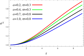
Figure 1: Plot of deformed radial metric (39) for the solution corresponding to $\tilde{\Pi}=0$.

We consider $f(\mathbb{R},\mathbb{T})$ model (9) to interpret both the obtained solutions, deformation functions and the complexity factor graphically. For this purpose, we choose multiple values of the coupling and decoupling parameters along with $\mathbb{C}_{1}=-0.003$, and explore different physical features of the considered compact star. Figure 1 exhibits plot of the deformed radial metric potential (39) and we observe its non-singular and increasing behavior for $0<r<\mathcal{R}$. The acceptability criteria of any gravitational model requires that the governing parameters, representing fluid distribution (such as energy density and pressure), must be maximum and finite in the core of astrophysical body, and monotonically decreasing towards its boundary. Figure 2 contains plots of the solution (41)-(44) and we observe its acceptable behavior. The energy density (left upper plot) is maximum in the middle and decreases with the increment in both the coupling and decoupling parameters. However, the pressure components show counter behavior as they increase by increasing $\alpha$ as well as $\varpi$. The radial pressure disappears at the boundary for all the considered values of these parameters. We observe from Figure 2 (last plot) that pressure anisotropy is zero at the center for $\alpha=0.2,~{}0.4,~{}0.7$ and vanishes throughout for $\alpha=1$ which confirms the system to be isotropic at this point.

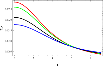
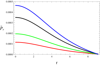
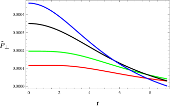
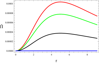
Figure 2: Plots of matter variables and anisotropy for the solution corresponding to $\tilde{\Pi}=0$.

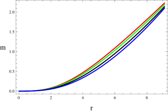
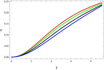
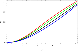
Figure 3: Plots of mass, compactness and redshift for the solution corresponding to $\tilde{\Pi}=0$.

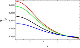
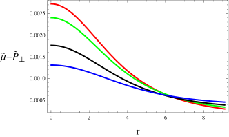
Figure 4: Plots of dominant energy conditions for the solution corresponding to $\tilde{\Pi}=0$.

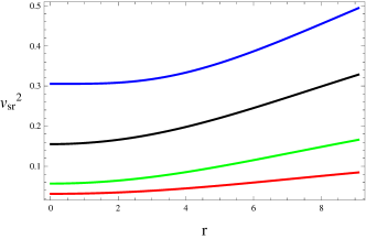
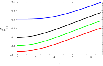
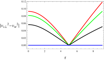
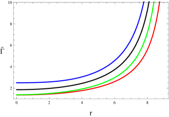
Figure 5: Plots of radial/tangential velocities, $|v_{s\bot}^{2}-v_{sr}^{2}|$ and adiabatic index for the solution corresponding to $\tilde{\Pi}=0$.

The mass of spherical geometry is presented in Figure 3, from which we observe that anisotropic system is more massive and dense as compared to isotropic analog. The other two plots also confirm the fulfillment of required limits of both the compactness and redshift. The state variables show positive trend, thus we only need to plot dominant energy conditions as $\tilde{\mu}-\tilde{P}_{r}\geq 0$ and $\tilde{\mu}-\tilde{P}_{\bot}\geq 0$. Figure 4 reveals the viability of our resulting solution as these bounds are satisfied. The stability is checked in Figure 5 through different approaches. According to the sound speed, the system is unstable near the core for $\alpha=0.2$ as $v_{s\bot}^{2}<0$, and stable everywhere for all other values of this parameter. However, Herrera’s cracking approach and the adiabatic index ensure the stability of spherical structure for all choices of $\alpha$ and $\varpi$ (lower two plots). The complexity factors (51) and (62) are plotted in Figure 6, and we notice that they decrease with the increment in coupling and decoupling parameters. This follows that $f(\mathbb{R},\mathbb{T})$ theory reduces the impact of complexity as compared to $\mathbb{GR}$.

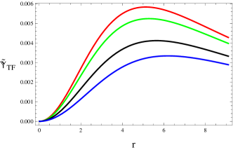
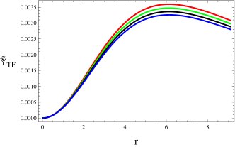
Figure 6: Plots of complexity factors (51) and (62).

We now explore physical characteristics of the solution corresponding to $\tilde{\mathbb{Y}}_{TF}=0$ by choosing $\mathbb{C}_{3}=-0.001$. The nature of deformed radial component is also found to be non-singular, as shown in Figure 7. Figure 8 demonstrates the plots of matter variables (66)-(68) and anisotropic pressure (69). They show the same behavior as we have found in the previous solution. The anisotropic factor vanishes at the center of star and then show negative trend towards the boundary, i.e., $\tilde{P}_{\bot}<\tilde{P}_{r}$. Figure 9 exhibits mass of the spherical geometry that decreases for higher values of parameters $\alpha$ and $\varpi$. The compactness and redshift also meet the required criteria (right and lower plots). The dominant energy conditions are plotted in Figure 10 whose fulfillment confirms viability of the corresponding solution as well as modified model (9). All the plots in Figure 11 reveal that our developed solution (66)-(69) is stable everywhere.

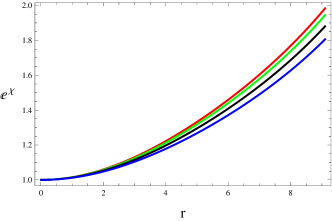
Figure 7: Plot of deformed radial metric (65) for the solution corresponding to $\tilde{\mathbb{Y}}_{TF}=0$.

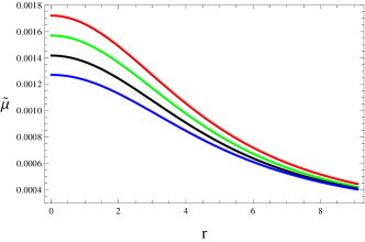
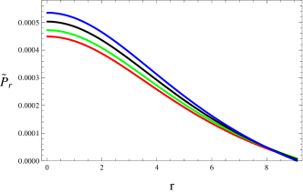
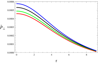
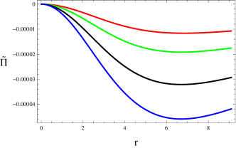
Figure 8: Plots of matter variables and anisotropy for the solution corresponding to $\tilde{\mathbb{Y}}_{TF}=0$.

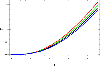
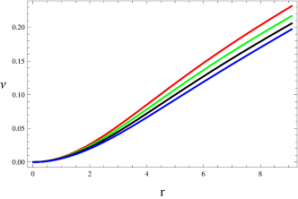
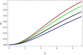
Figure 9: Plots of mass, compactness and redshift for the solution corresponding to $\tilde{\mathbb{Y}}_{TF}=0$.

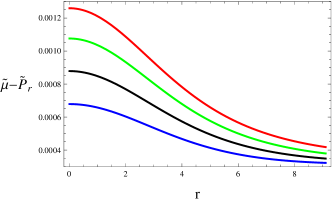
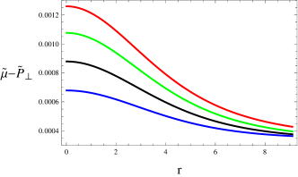
Figure 10: Plots of dominant energy conditions for the solution corresponding to $\tilde{\mathbb{Y}}_{TF}=0$.

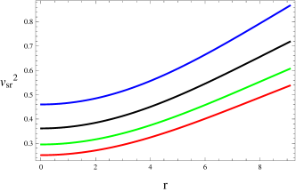
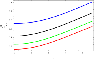
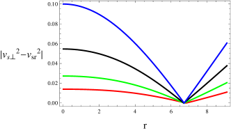
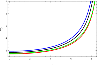
Figure 11: Plots of radial/tangential velocities, $|v_{s\bot}^{2}-v_{sr}^{2}|$ and adiabatic index for the solution corresponding to $\tilde{\mathbb{Y}}_{TF}=0$.

7 Conclusions

In this paper, we have extended the existing solutions corresponding to self-gravitating anisotropic sphere by adding an extra source with the help of gravitational decoupling in $f(\mathbb{R},\mathbb{T})=\mathbb{R}+2\varpi\mathbb{T}$ gravity. We have formulated the modified field equations comprising the effects of both sources and then separated them into two sets through the MGD technique. Both the obtained sectors correspond to the original anisotropic and the additional source, respectively. To deal with the first set, we have used

$$\sigma(r)=\ln\bigg{\{}\mathcal{B}^{2}\bigg{(}1+\frac{r^{2}}{\mathcal{A}^{2}}\bigg{)}\bigg{\}},\quad\xi(r)=e^{-\chi(r)}=\frac{\mathcal{A}^{2}+r^{2}}{\mathcal{A}^{2}+3r^{2}},$$

and metric potentials of Tolman IV ansatz, leading to two different solutions. The unknowns involving in these solutions have been calculated through boundary conditions for the mass and radius of $4U1820-30$. The second sector (23)-(25) contains four unknowns, thus we have implemented extra constraints on the newly added source $\mathfrak{A}_{\zeta\eta}$. We have considered vanishing of the effective anisotropy to obtain the first solution which leads to an isotropic system for $\alpha=1$. The other solution is obtained by taking into the account that complexity of the original and additional matter sources cancel out the effect of each other.

The physical features of the obtained results have been analyzed by taking $\alpha=0.2,~{}0.4,~{}0.7,~{}1$ and $\varpi=0.3,~{}0.8$. The acceptable behavior of the corresponding state variables ((41)-(43) and (66)-(68)), anisotropy ((44) and (69)) and the energy conditions (72) have been observed for specific values of the integration constants. We have also found fulfillment of the required limit for redshift and compactness (Figures 3 and 9). It is noticed that the solution corresponding to $\tilde{\Pi}=0$ produces more dense stellar structure for all values of $\alpha$ and $\varpi$, as compared to the other solution. The deformation functions (38) and (64) are zero at the center and exhibit positive behavior throughout. We have checked stability of both the extended solutions through multiple approaches such as the sound speed, cracking approach and the adiabatic index, and their corresponding criteria is fulfilled, hence these solutions are stable. It must be mentioned that our solutions are consistent with $\mathbb{GR}$ [29]. Moreover, the solution corresponding to $\tilde{\Pi}=0$ shows compatible behavior with the Brans-Dicke gravity [31], as it shows unstable behavior for $\alpha=0.2$ in that case as well (Figure 5). Finally, all of our results reduce to $\mathbb{GR}$ for $\varpi=0$.

Data Availability Statement: This manuscript has no associated data.

References

[1] Capozziello, S. et al.: Class. Quantum Grav. 25(2008)
085004; Nojiri, S. et al.: Phys. Lett. B 681(2009)74.
[2] de Felice, A. and Tsujikawa, S.: Living Rev.
Relativ. 13(2010)3; Nojiri, S. and Odintsov, S.D.: Phys.
Rep. 505(2011)59.
[3] Sharif, M. and Kausar, H.R.: J. Cosmol. Astropart. Phys.
07(2011)022; Sharif, M. and Yousaf, Z.: Astrophys. Space
Sci. 354(2014)471.
[4] Astashenok, A.V., Capozziello, S. and Odintsov, S.D.: J. Cosmol. Astropart. Phys. 01(2015)001;
Phys. Lett. B 742(2015)160.
[5] Bertolami, O. et al.: Phys. Rev. D 75(2007)104016.
[6] Harko, T. et al.: Phys. Rev. D 84(2011)024020.
[7] Deng, X.M. and Xie, Y.: Int. J. Theor. Phys.
54(2015)1739.
[8] Houndjo, M.J.S.: Int. J. Mod. Phys. D
21(2012)1250003.
[9] Das, A. et al.: Phys. Rev. D 95(2017)124011.
[10] Sharif, M. and Siddiqa, A.: Eur. Phys. J. Plus 133(2018)226;
Sharif, M. and Nawazish, I.: Astrophys. Space Sci.
363(2018)67; Sharif, M. and Waseem, A.: Eur. Phys. J. C
78(2018)868.
[11] Rej, P., Bhar, Piyali. and Govender, M.: Eur. Phys. J. C
81(2021)316; Zubair, M. et al.: New Astron.
88(2021)101610; Azmata, H. and Zubair M.: Eur. Phys. J.
Plus 136(2018)112.
[12] Ovalle, J.: Mod. Phys. Lett. A 23(2008)3247.
[13] Ovalle, J. and Linares, F.: Phys. Rev. D 88(2013)104026.
[14] Casadio, R., Ovalle, J. and Da Rocha, R.: Class. Quantum Grav. 32(2015)215020.
[15] Ovalle, J. et al.: Eur. Phys. J. C 78(2018)960.
[16] Sharif, M. and Sadiq, S.: Eur. Phys. J. C 78(2018)410.
[17] Sharif, M. and Saba, S.: Eur. Phys. J. C 78(2018)921; Chin. J. Phys. 59(2019)481;
Sharif, M. and Waseem, A.: Ann. Phys. 405(2019)14.
[18] Gabbanelli, L., Rincón, Á. and Rubio, C.: Eur. Phys. J. C 78(2018)370.
[19] Estrada, M. and Tello-Ortiz, F.: Eur. Phys. J. Plus 133(2018)453.
[20] Hensh, S. and Stuchlík, Z.: Eur. Phys. J. C 79(2019)834.
[21] Sharif, M. and Ama-Tul-Mughani, Q.: Int. J. Geom. Methods Mod. Phys.
16(2019)1950187; Mod. Phys. Lett. A
35(2020)2050091.
[22] Sharif, M. and Majid, A.: Chin. J. Phys.
68(2020)406; Phys. Dark Universe 30(2020)100610.
[23] Sharif, M. and Naseer, T.: Chin. J. Phys.
73(2021)179; Int. J. Mod. Phys. D 31(2022)2240017;
Phys. Scr. 97(2022)055004; Pramana 96(2022)119;
Naseer, T. and Sharif, M.: Universe 8(2022)62.
[24] Herrera, L.: Phys. Rev. D 97(2018)044010.
[25] Herrera, L., Di Prisco, A. and Ospino, J.: Phys. Rev. D
98(2018)104059.
[26] Yousaf, Z., Bhatti, M.Z. and Naseer, T.: Eur. Phys. J. Plus
135(2020)353; Phys. Dark Universe 28(2020)100535;
Int. J. Mod. Phys. D 29(2020)2050061; Ann. Phys.
420(2020)168267.
[27] Yousaf, Z. et al.: Phys. Dark Universe
29(2020)100581; Yousaf, Z. et al.: Mon. Not. R. Astron.
Soc. 495(2020)4334; Sharif, M. and Naseer, T.: Chin. J.
Phys. 77(2022)2655; Eur. Phys. J. Plus
137(2022)947.
[28] Carrasco-Hidalgo, M. and Contreras, E.: Eur. Phys. J. C
81(2021)757; Andrade, J. and Contreras, E.: Eur. Phys. J. C
81(2021)889; Arias, C. et al.: Ann. Phys.
436(2022)168671.
[29] Casadio, R. et al.: Eur. Phys. J. C
79(2019)826.
[30] Maurya, S.K. and Nag, R.: Eur. Phys. J. C
82(2022)48; Maurya, S.K. et al.: Eur. Phys. J. C
82(2022)100.
[31] Sharif, M. and Majid, A.: Eur. Phys. J. Plus
137(2022)114.
[32] Houndjo, M.J.S. and Piattella, O.F.: Int. J. Mod. Phys. D
2(2012)1250024.
[33] Moraes, P.H.R.S., Correa, R.A.C. and Ribeiro, G.: Eur. Phys. J. C
78(2018)192.
[34] Einstein, A.: Ann. Math. 40(1939)922.
[35] Güver, T., Wroblewski, P., Camarota, L. and
Özel, F.: Astrophys. J. 719(2010)1807.
[36] Buchdahl, H.A.: Phys. Rev. 116(1959)1027.
[37] Ivanov, B.V.: Phys. Rev. D 65(2002)104011.
[38] Abreu, H., Hernandez, H. and Nunez, L.A.: Class. Quantum Gravit.
24(2007)4631.
[39] Herrera, L.: Phys. Lett. A 165(1992)206.
[40] Heintzmann, H. and Hillebrandt, W.: Astron. Astrophys.
38(1975)51.