AutoPV: Automated photovoltaic forecasts with limited information using an ensemble of pre-trained models

Abstract

Accurate PV power generation forecasting is vital for the efficient operation of Smart Grids. The automated design of such accurate forecasting models for individual PV plants includes two challenges: First, information about the PV mounting configuration (i.e. inclination and azimuth angles) is often missing. Second, for new PV plants, the amount of historical data available to train a forecasting model is limited (cold-start problem). We address these two challenges by proposing a new method for day-ahead PV power generation forecasts. The proposed AutoPV method is a weighted ensemble of forecasting models that represent different PV mounting configurations. This representation is achieved by pre-training each forecasting model on a separate PV plant and by scaling the model’s output with the peak power rating of the corresponding PV plant. To tackle the cold-start problem, we initially weight each forecasting model in the ensemble equally. To tackle the problem of missing information about the PV mounting configuration, we use new data that become available during operation to adapt the ensemble weights to minimize the forecasting error. The proposed AutoPV method is advantageous as the unknown PV mounting configuration is implicitly reflected in the ensemble weights, and only the PV plant’s peak power rating is required to re-scale the ensemble’s output. The ensemble approach also allows to represent PV plants with panels distributed on different roofs with varying alignments, as these mounting configurations can be reflected proportionally in the weighting. Additionally, the required computing memory is decoupled when scaling AutoPV to several hundreds of PV plants, which is beneficial in Smart Grid environments with limited computing capabilities. For a real-world data set with 11 PV plants, the accuracy of AutoPV is comparable to an individual model trained on two years of data and outperforms an incrementally trained individual model.

Keywords photovoltaic forecasting  $\cdot$ ensemble  $\cdot$ cold-start  $\cdot$ automated design  $\cdot$ online operation

1 Introduction

The Paris Climate Agreement targets net-zero emissions of the energy system by 2050 [1]. This target requires reducing primary energy demand, increasing energy efficiency, and increasing the share of renewables in electricity generation. The latter endangers grid stability, as the fluctuating and non-controllable production behavior of renewables may put the frequency stability under pressure or lead to power line congestion. Hence, a Smart Grid is required that integrates communication, measurement, control, and automation technology. This integration enables the Smart Grid to monitor local power grid conditions in real-time and enables full utilization of the grid capacity by balancing demand and supply [2]. The full utilization and balance of supply and demand are realizable by using demand-side management and proactive supply control. Yet, both rely on accurate demand and supply forecasts [3].

In this context, the automated design of such accurate forecasting models for the decentral generation of PV power includes two challenges related to missing information about an individual PV plant: First, the PV mounting configuration characterized by inclination and azimuth angles is difficult to obtain as both are often incompletely documented or roughly approximated. Especially for PV plants with panels distributed on different roofs with varying alignments, often only the total peak power rating of the PV plant is known. This missing documentation limits the large-scale application of forecasting methods that rely on information about the PV mounting configuration (e.g. [4, 5]). Second, often historical data for training the forecasting model are not available (cold-start problem). For example, for newly built PV plants, nearly no data are available. Consequently, data-intensive forecasting methods such as deep learning methods (e.g. [6, 7, 8]) are not directly applicable to new PV plants.

Therefore, the present paper addresses these two challenges by proposing a new method for day-ahead PV forecasts called AutoPV. This method only requires the new PV plant’s peak power rating, is applicable without any training data of the new plant, and adapts itself during operation. Our proposed forecasting method AutoPV is based on creating an ensemble of multiple forecasting models. The models in the ensemble pool are pre-trained on historical data of different PV plants of the same region with various mounting configurations that are scaled with the corresponding peak power rating. Thus, the model pool contains expert models for various PV mounting configurations. To tackle the cold-start problem where no data of the PV plant are available, each model in the ensemble contributes equally to the forecast. During the operation, new data are collected and used to adapt the ensemble weights. More specifically, the contribution of each model in the ensemble pool is adapted such that the weighted sum optimally fits the new PV plant. Thereby, the unknown PV mounting configuration is implicitly reflected in the ensemble weights. Also, PV plants with panels distributed on different roofs with varying alignments can be reflected proportionally in the weighting.

Regarding the taxonomy of automated forecasting pipelines described in [9], our method covers all 5 sections, i.e., data pre-processing, feature engineering, hyperparameter optimization, forecasting method selection, and forecast ensembling. The organization of this workflow using a machine learning pipeline, as well as automatic model design and selection along with continuous adaptation during operation, corresponds to Automation level 3 [10]. For creating automated forecasting pipelines, generic frameworks such as TPOT [11] exist, but they are not adapted to a specific domain and thus cannot leverage prior knowledge on PV forecasting.

The remainder of this paper is organized as follows. We describe the methodology of the proposed PV power generation forecasting method in Section 2, evaluate it in Section 3, discuss the results in Section 4 and give a conclusion and an outlook in Section 5.

2 Design of the AutoPV method

As described in the introduction, unknown PV mounting configurations characterized by inclination and azimuth angles are challenging for the design of a PV forecasting model. Thus, the underlying idea of the proposed AutoPV method is that each new PV mounting configuration can be described by the sum of weighted elements from a sufficiently diverse pool of forecasting models of the same region.

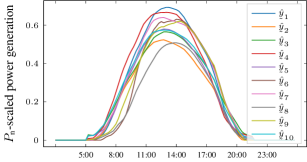
(a) The result of the first step is the scaled ensemble pool model forecasts $\hat{\underaccent{\tilde}{y}}_{n}$.

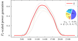
(b) The result of the second step is the scaled ensemble forecast $\hat{\underaccent{\tilde}{y}}$.

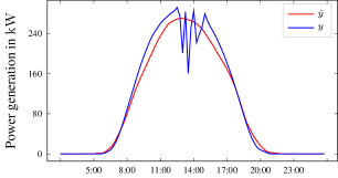
(c) The result of the third step is the re-scaled ensemble forecast $\hat{{y}}$. Additionally, this plot shows the measurement $y$ with cloud overflight between 12:00 and 15:00. The ensemble forecast is based on a day-ahead radiation forecast that also considers cloud cover but with lower spatial and temporal resolution.

Figure 1: The three steps of the proposed PV ensemble forecasting method exemplified for PV plant no. 11.

The proposed AutoPV method incorporates three steps: i) create the model pool, ii) form the ensemble forecast by an optimally weighted sum of the scaled forecasts, and iii) re-scale the ensemble forecast with the new PV plant’s peak power rating. These three steps are detailed in the following and Figure 1 provides exemplary results of these three steps.

2.1 Creation of the ensemble pool models

Each model in the ensemble pool is equally designed. However, each model is pre-trained on historical data of an individual PV plant. Thus, the ensemble model pool covers a diverse set of PV mounting configurations. Each model is based on a machine learning pipeline, including pre-processing and feature extraction, an automatically designed regression estimator, and a set of rules reflecting prior knowledge. First, we describe the machine learning pipeline and afterward the automated regression estimator design.

Machine learning pipeline

For each model $n\ldots N$, we pre-process the training data by scaling the PV power generation measurement according to the peak power rating $P_{\text{n},n}$ of the corresponding PV plant

$$\underaccent{\bar}{y}_{n}[k]=\frac{y_{n}[k]}{P_{\text{n},n}},$$ (1)

where $k\in\mathbb{N}^{K}$ is the sample index. In contrast to the PV mounting configurations, we assume that $P_{\text{n},n}$ is a parameter of the PV plants that can be reliably determined. However, scaling with $P_{\text{n},n}$ does not lead to aligned PV power generation curves (see 1(a)). This is because the mounting configuration of a PV plant influences the maximum possible amount of generated power. For example, a PV plant oriented to the south generates more than a PV plant oriented to the west. In addition, global radiation’s seasonal and weather-dependent intensity also affects the distance between the PV power output and the plant’s peak power rating.

As inputs, each regression estimator uses global radiation $\hat{G}$ considering cloud cover and air temperature $\hat{T}$ forecasts, and the corresponding second-order polynomial and interaction features. Additionally, we use sin-cos encoded cyclic features of the month and minute of the day to represent seasonal information:

$$x_{\text{s12}}[k] =\sin(2\pi\cdot\text{month}[k]\cdot 12^{-1}),$$ (2)

$$x_{\text{c12}}[k] =\cos(2\pi\cdot\text{month}[k]\cdot 12^{-1}),$$ (3)

$$x_{\text{s1440}}[k] =\sin(2\pi\cdot\text{minute}[k]\cdot 1440^{-1}),$$ (4)

$$x_{\text{c1440}}[k] =\cos(2\pi\cdot\text{minute}[k]\cdot 1440^{-1}).$$ (5)

The periodicity of these trigonometric functions establishes similarities between temporally related samples, while the sin-cos pair is necessary because, otherwise, the encoding would be ambiguous at several points.

The resulting regression estimator for plant $n$ in the ensemble pool is a function of

$$\begin{split}\hat{\underaccent{\bar}{y}}_{n}[k]=f&\left(\hat{G}^{2}[k],\hat{G}[k],(\hat{G}\cdot\hat{T})[k],\hat{T}[k],\hat{T}^{2}[k],\right.\\ &\left.\vphantom{\hat{G}^{2}[k],\hat{G}[k],(\hat{G}\cdot\hat{T})[k],\hat{T}[k],\hat{T}^{2}[k]}x_{\text{s12}}[k],x_{\text{c12}}[k],x_{\text{s1440}}[k],x_{\text{c1440}}[k],\boldsymbol{p}\right),\end{split}$$ (6)

where the parameters $\boldsymbol{p}$ are determined by training the machine learning pipeline on historical data.

To consider prior knowledge in forecasting PV power generation, we use two rules. First, no PV power is generated if there is no solar radiation. Second, negative PV power generation is not possible. Consequently, we drop the night times from the training data and set the forecast to zero during these times. Furthermore, the negative values in the forecast are set to zero.

Incorporating these two steps leads to

$$\hat{\underaccent{\tilde}{y}}_{n}[k]=\begin{cases*}\hat{\underaccent{\bar}{y}}_{n}[k],&if $\hat{G}[k]>0$ and $\hat{\underaccent{\bar}{y}}_{n}[k]>0$,\\ 0&otherwise,\\ \end{cases*}$$ (7)

as the final step in the machine learning pipeline.

Automated regression estimator design

For automatically designing the regression estimator, we define a CASH problem. In the CASH problem, we aim to minimize the machine learning pipeline’s MSE

$$\text{MSE}=\frac{1}{K}\sum_{k=1}^{K}\left(\hat{\underaccent{\tilde}{y}}_{n}[k]-\underaccent{\bar}{y}_{n}[k]\right)^{2},$$ (8)

by selecting the optimal configuration, i.e., the optimal regression algorithm and the corresponding optimal hyperparameters. The configuration space is shown in Table 1, which is explored during CASH using Bayesian optimization. Each configuration trial is trained on a training data set and assessed on a hold-out validation data set.

Implementation

The machine learning pipeline is implemented using the Python package pyWATTS [12] and the regression estimators are implemented using the Python package scikit-learn [13]. For solving the CASH problem, we use the Python package Ray Tune [14] with the hyperopt [15] search algorithm. The CASH is automatically stopped if the MSE plateaus across trials, i.e., the MSE of the top 10 trials have a standard deviation of less than 0.001 with a patience of 15 trials.

Table 1: The configuration space for the automated regression estimator design using CASH in scikit-learn [13] naming convention.

Regression estimator Hyperparameter Value range Ridge alpha $[0.05,1]$ MLPRegressor activation $\{\texttt{logistic, tanh, relu}\}$ hidden_layer_sizes $\{([10,100])$ $\phantom{\{}([10,100],[10,100])$ $\phantom{\{}([10,100],[10,100],[10,100])\}$ GradientBoostingRegressor learning_rate $[0.01,1]$ n_estimators $[10,300]$ max_depth $[1,10]$ RandomForestRegressor n_estimators $[10,300]$ max_depth $[1,10]$ SVR C $[0.01,10]$ epsilon $[0.001,1]$

2.2 Optimal weighting of the ensemble pool models

The idea of creating an ensemble is to increase the robustness of data-driven models by combining multiple forecasts from a pool of different models [16]. Apart from weighting each model in the pool equally (averaging), one may give more weight to models from which we expect good performance and give less weight to models from which we expect poor performance, i.e.,

$$\hat{\underaccent{\tilde}{y}}[k]=\sum^{N}_{n=1}w_{n}\cdot\hat{\underaccent{\tilde}{y}}_{n}[k]$$ (9)

with $w_{n}$ being the weight of the $n$-th model in the ensemble pool.

To find the weights of the ensemble, we distinguish the initialization and the operation phase. In the initialization phase, historical power generation data for the new PV plant are not available. Thus, we weight each model in the ensemble pool equally. During the operation, new data are used to cyclically adapt the ensemble weights in such a way that they optimally fit the new PV plant (see 1(b)). For optimal weighting, we vary the weights of the ensemble pool models $\boldsymbol{w}$ to minimize the MSE over the $K$ most recent samples of the $P_{\text{n}}$-scaled data $\underaccent{\tilde}{\boldsymbol{y}}$. With (9), this results in the optimization problem

$$\begin{split}\min_{\boldsymbol{w}}\frac{1}{K}\sum^{K}_{k=1}\left(\hat{\underaccent{\tilde}{y}}[k]-\underaccent{\bar}{y}[k]\right)^{2}\\ \textrm{s.t.}\quad\boldsymbol{w}\in[0,1],\sum^{N}_{n=1}w_{n}=1,\end{split}$$ (10)

which we solve using the least squares implementation of the Python package SciPy [17], and normalize the weights afterward to hold the constraints.

Note that the cycle length $C$ of the adaption routine and the number of considered samples $K$ are hyperparameters of the proposed AutoPV.

2.3 Transformation of the ensemble forecast to the new PV plant

The last step yields the final ensemble forecast, shown in 1(c)). To this end, it re-scales the weighted average of the ensemble according to the peak power rating $P_{\text{n,new}}$ of the new PV plant:

$$\hat{y}[k]=\hat{\underaccent{\tilde}{y}}[k]\cdot P_{\text{n,new}}.$$ (11)

3 Evaluation

We evaluate the proposed AutoPV method on a real-world data set containing three years (2018 – 2020) of quarter-hourly power generation measurement ($\mathrm{kW}\text{\,}\mathrm{h}$) from 11 PV plants located in southern Germany. For better interpretability, we transform the energy generation time series into the mean power generation time series

$$\overline{P}[k]=\frac{\Delta E[k]}{t_{k}},$$ (12)

where $\Delta E[k]$ is the energy generated in the sample period $t_{k}$ ($1/$\mathrm{h}$$). Additionally, we use corresponding day-ahead weather forecasting data.

We pre-train the ensemble pool models with the data from 2018 and 2019, and assess the proposed AutoPV method with all samples of 2020. In pre-training, the automated regression estimator design via CASH predominately creates a MLP regressor with two or three hidden layers and the ReLU activation function.

In the following, we first evaluate the performance of AutoPV and then the consistency of AutoPV’s ensemble optimization.

Performance evaluation

We evaluate the performance of AutoPV using a plant-wise leave-one-out evaluation. That is, we assess the forecasting error of the proposed AutoPV method on each PV plant while excluding this plant from the ensemble model pool. Since the PV plants in the data set have different peak power ratings and would differently influence the MAE, we use the nMAE as assessment metric:

$$\text{nMAE}=\frac{\sum_{k=1}^{K}\left|\hat{y}[k]-y[k]\right|}{\sum_{k=1}^{K}{y[k]}}.$$ (13)

In the evaluation, we start with equal ensemble weights and adapt them every 28 days based on the samples obtained in the most recent 28 days ($C=28,K=28\cdot 96$).

We compare the performance of the proposed AutoPV method with three methods. The first method reflects an ideal situation in the sense that we assume that there are two years of historical data available (2018, 2019) to train an individual model (IM-HDA) for the considered PV plant. The second method is an averaging ensemble, which reflects the initialization phase of AutoPV without adapting the weights during operation. As a third method, we train an individual model incrementally (IM-IT) every 28 days. More specifically, the IM-IT uses all data of the testing data set (2020) that is obtained until the $l$-th adaption ($C=28,K=l\cdot 28\cdot 96,l=[1,2,\ldots]$). The performance comparison of IM-IT, Averaging, and AutoPV with the IM-HDA is unfair in terms of training data because the IM-HDA is trained on data of the PV plant that is unavailable to them.

In the performance evaluation, we make three observations. First, considering the average assessment metric over all plants $\overline{\text{nMAE}}$, we see that the proposed AutoPV method comes close to the ideal situation IM-HDA. Second, regarding the cold-start problem, the proposed AutoPV method outperforms the IM-IT (compare Table 2). Third, PV plant no. 7 has multiple dips in September and October, as well as a complete shutdown of this plant in May (see Figure 2), and the nMAE of all methods is comparatively high for this plant.

Table 2: The nMAE of the proposed AutoPV method compared to the historical data available model (IM-HDA), the averaging ensemble, and the incrementally trained individual model (IM-IT) in the plant-wise leave-one-out evaluation.

IM-HDA IM-IT Averaging AutoPV Training data 2 years 1 month none none Adaption cycle $C$ none 28d none 28d Adaption samples $K$ none $l\cdot 28\cdot 96$ none $28\cdot 96$ $\text{nMAE}_{1\phantom{1}}$ 0.308 0.332 0.367 0.278 $\text{nMAE}_{2\phantom{1}}$ 0.298 0.321 0.302 0.299 $\text{nMAE}_{3\phantom{1}}$ 0.271 0.310 0.314 0.289 $\text{nMAE}_{4\phantom{1}}$ 0.316 0.349 0.385 0.291 $\text{nMAE}_{5\phantom{1}}$ 0.325 0.343 0.353 0.335 $\text{nMAE}_{6\phantom{1}}$ 0.327 0.322 0.299 0.289 $\text{nMAE}_{7\phantom{1}}$ 0.418 0.588 0.491 0.448 $\text{nMAE}_{8\phantom{1}}$ 0.280 0.310 0.280 0.277 $\text{nMAE}_{9\phantom{1}}$ 0.362 0.424 0.502 0.416 $\text{nMAE}_{10}$ 0.307 0.365 0.364 0.318 $\text{nMAE}_{11}$ 0.311 0.471 0.324 0.311 $\overline{\text{nMAE}}_{\phantom{1}\phantom{1}}$ 0.320 0.376 0.362 0.323
bolt: winner of fair comparison in terms of training data; bolt&italics: winner of unfair comparison

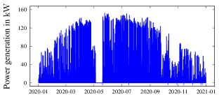
Figure 2: Shutdowns and partial shutdowns of PV plant no. 7 lead to sudden dips in the generated power.

Consistency evaluation

We evaluate the consistency of the AutoPV ensemble optimization as described above, except that the ensemble model pool includes all PV plants, i.e., the IM-HDA is available in the pool. Hence, a consistent ensemble optimization should give high weight to the IM-HDA.

(a) PV plant no. 5 is rather similar compared to other plants.

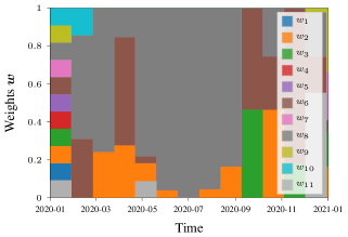
(b) PV plant no. 8 is rather unique compared to other plants.

Figure 3: Weight development in the consistency evaluation.

Figure 3 shows the exemplary weight evolution of PV plant no. 5 and PV plant no. 8. PV plant no. 5 represents a plant whose power generation curve is rather similar to other plants, while PV plant no. 8 reflects a rather unique power generation curve (compare in 1(a)).

In the consistency evaluation, we make three observations. First, after the initialization phase, the weights change significantly. Second, the more unique the power generation curve of a PV plant, the clearer the weighting towards the IM-HDA (compare 3(a) and 3(b), where for PV plant no. 5 the weight $w_{5}$ and for PV plant no. 8 the weight $w_{8}$ corresponds to the respective IM-HDA). Third, the weighting is generally clearer towards the IM-HDA in the summer than in the winter.

4 Discussion

This section discusses the results, limitations, and benefits of the proposed AutoPV method.

With regard to the results, we discuss two aspects: First, we observe that the proposed AutoPV method and the ideal IM-HDA perform almost similarly. Thus, we conclude that any PV mounting configuration in the given dataset can be represented by recombining the ensemble pool models’ forecasts. This recombination via the ensemble weights also allows to represent PV plants with panels distributed on different roofs with varying alignments. More specifically, the AutoPV method is not limited to represent a single PV mounting configuration. Instead, the mounting configurations of PV panels distributed on different roofs can be reflected proportionally in the weighting. Second, we observe that the proposed AutoPV method outperforms the IM-IT. This might be explained by the fact that the pre-trained ensemble pool models already reflect the entire seasonality, whereas the IM-IT learns it with a delay. However, the forecasting accuracy of both is harmed by dips in the generated PV power, as this sudden change is only captured with a delay by the cyclic adaptation.

Regarding the limitations, we discuss the creation of the ensemble pool. For representing a new PV plant by recombining the ensemble pool models’ forecasts, they must be diverse with respect to the PV mounting configurations. To create a diverse ensemble model pool, we can use prior knowledge or select a diverse set of curves after the $P_{\text{n}}$-scaling (see 1(a)). However, we cannot guarantee that an ensemble pool of 10 models is sufficiently diverse to represent all alignment combinations. This limitation can be overcome by automatically designing an individual model for the new PV plant after a full year and adding it to the ensemble pool.

The proposed AutoPV method is beneficial because it is universally applicable and achieves promising results with only 10 representative models in the ensemble pool. As scaling AutoPV to several hundred PV plants still requires only the 10 ensemble pool models to be stored in the computing memory, and the weight adaptation effort is very low, AutoPV is advantageous for Smart Grid environments with limited computing capabilities. Moreover, the universality of our approach allows us to use arbitrary complex models in the ensemble pool.

5 Conclusion and outlook

Designing accurate PV power generation forecasting models for Smart Grid operation includes two challenges: The first is the missing information about the PV mounting configuration (inclination and azimuth angles). The second is the limited availability of historical data to train the forecasting model (cold-start problem). To address both challenges, we propose a new method for day-ahead PV forecasts that only requires the new PV plant’s peak power rating, that is applicable without any training data of the new plant, and that adapts itself during operation (Automation level 3 [10]). The new AutoPV method is an automated forecasting pipeline [9] based on an ensemble with a pool of pre-trained models that represent various PV mounting configurations. While initially, each model in the ensemble pool contributes equally to the forecast, the contribution of each model is adapted during operation using the least squares method such that the weighted sum optimally fits the new PV plant. Hence, the AutoPV method is also applicable to PV plants with panels distributed on different roofs with varying alignments, as these mounting configurations can be reflected proportionally in the weighting.

The evaluation on real-world data shows that the proposed AutoPV method outperforms an incrementally trained individual model. It achieves comparable performance to the ideal situation of having two years of historical data available to train an individual model. The evaluation also shows that for reliable and automated online operation, it is necessary to consider PV power generation dips caused by technical defects, scheduled maintenance, or soiling. Therefore, the AutoPV method will be extended in future research to include a drift detection method and consider the PV plant’s efficiency with additional weight in the ensemble optimization.

References

- [1] UNFCCC “Paris Agreement” In United Nations Treaty Collection Chapter XXVII 7. d, 2015
- [2] Xi Fang, Satyajayant Misra, Guoliang Xue and Dejun Yang “Smart Grid – The new and improved power grid: A survey” In IEEE Communications Surveys & Tutorials 14.4, 2012, pp. 944–980
- [3] Lars Dannecker “Energy time series forecasting” Wiesbaden, Germany: Springer, 2015
- [4] Oscar Perpiñán Lamigueiro “solaR: Solar radiation and photovoltaic systems with R” In Journal of Statistical Software 50.9 American Statistical Association, 2012, pp. 1–32
- [5] William F. Holmgren, Clifford W. Hansen and Mark A. Mikofski “pvlib Python: A Python package for modeling solar energy systems” In Journal of Open Source Software 3.29 The Open Journal, 2018, pp. 884
- [6] Mohamed Abdel-Basset, Hossam Hawash, Ripon K Chakrabortty and Michael Ryan “PV-Net: An innovative deep learning approach for efficient forecasting of short-term photovoltaic energy production” In Journal of Cleaner Production 303 Elsevier, 2021, pp. 127037
- [7] Muhammad Aslam, Seung-Jae Lee, Sang-Hee Khang and Sugwon Hong “Two-stage attention over LSTM with Bayesian optimization for day-ahead solar power forecasting” In IEEE Access 9, 2021, pp. 107387–107398
- [8] Kejun Wang, Xiaoxia Qi and Hongda Liu “A comparison of day-ahead photovoltaic power forecasting models based on deep learning neural network” In Applied Energy 251.C, 2019, pp. 1–1
- [9] Stefan Meisenbacher et al. “Review of automated time series forecasting pipelines” In WIREs Data Mining and Knowledge Discovery 12.6, 2022, pp. e1475
- [10] Stefan Meisenbacher et al. “Concepts for automated machine learning in Smart Grid applications” In Proceedings - 31. Workshop Computational Intelligence : Berlin, 25. - 26. November 2021. Hrsg.: H. Schulte; F. Hoffmann; R. Mikut KIT Scientific Publishing, 2021, pp. 11–35
- [11] Randal S. Olson, Nathan Bartley, Ryan J. Urbanowicz and Jason H. Moore “Evaluation of a tree-based pipeline optimization tool for automating data science” In Proceedings of the Genetic and Evolutionary Computation Conference 2016, GECCO ’16 Denver, Colorado, USA: ACM, 2016, pp. 485–492
- [12] Benedikt Heidrich et al. “pyWATTS: Python workflow automation tool for time series” In arXiv:2106.10157, 2021
- [13] F. Pedregosa et al. “Scikit-learn: Machine learning in Python” In Journal of Machine Learning Research 12, 2011, pp. 2825–2830
- [14] Richard Liaw et al. “Tune: A research platform for distributed model selection and training” In arXiv:1807.05118, 2018
- [15] James Bergstra, Daniel Yamins and David Cox “Making a science of model search: Hyperparameter optimization in hundreds of dimensions for vision architectures” In International conference on machine learning, 2013, pp. 115–123 PMLR
- [16] David Shaub “Fast and accurate yearly time series forecasting with forecast combinations” In International Journal of Forecasting 36.1, 2020, pp. 116–120
- [17] Pauli Virtanen et al. “SciPy 1.0: Fundamental algorithms for scientific computing in Python” In Nature Methods 17, 2020, pp. 261–272