On Computing the Vertex Connectivity of 1-Plane Graphs

Abstract

A graph is called 1-plane if it has an embedding in the plane where each edge is crossed at most once by another edge. A crossing of a 1-plane graph is called an $\times$-crossing if there are no other edges connecting the endpoints of the crossing (apart from the crossing pair of edges). In this paper, we show how to compute the vertex connectivity of a 1-plane graph $G$ without $\times$-crossings in linear time.

To do so, we show that for any two vertices $u,v$ in a minimum separating set $S$, the distance between $u$ and $v$ in an auxiliary graph $\Lambda(G)$ (obtained by planarizing $G$ and then inserting into each face a new vertex adjacent to all vertices of the face) is small. It hence suffices to search for a minimum separating set in various subgraphs $\Lambda_{i}$ of $\Lambda(G)$ with small diameter. Since $\Lambda(G)$ is planar, the subgraphs $\Lambda_{i}$ have small treewidth. Each minimum separating set $S$ then gives rise to a partition of $\Lambda_{i}$ into three vertex sets with special properties; such a partition can be found via Courcelle’s theorem in linear time.

1 Introduction

The class of planar graphs, which are graphs that can be drawn on the plane without crossings, is fundamental to both graph theory and graph algorithms. Many problems can be more efficiently solved in planar graphs than in general graphs. However, real-world graphs, such as social networks and biological networks, are typically non-planar. But they are often near-planar, i.e., close to planar in some sense. One such graph class is the 1-planar graphs, i.e., graphs that can be drawn on the plane such that each edge is crossed at most once. Introduced in 1965 [28], both structural and algorithmic properties of 1-planar graphs have been studied extensively, see [17, 21] for overviews.

In this paper, we look at the problem of vertex connectivity for 1-planar graphs. The problem of vertex connectivity is fundamental in graph theory: given a connected graph $G$, what is the size (denoted by $\kappa(G)$) of the smallest separating set, i.e., set of vertices whose removal makes $G$ disconnected? Vertex connectivity has many applications, e.g. in network reliability and for measuring social cohesion.

Known Results:

For an $n$-vertex $m$-edge graph $G$, one can test in linear (i.e. $O(m{+}n)$) time whether $\kappa(G)\geq 1$ with a graph traversal algorithm. In 1969, Kleitman [20] showed how to test $\kappa(G)\leq k$ in time $O(k^{2}nm)$. Subsequently, [29] and [18] presented linear-time algorithms to decide $k$-connectivity for $k=2$ and $k=3$ respectively. (Some errors in [18] were corrected in [15].) For $\kappa(G)=4$, the first $O(n^{2})$ algorithm was by Kanevsky and Ramachandran [19]. For $\kappa(G)\in O(1)$, the first $O(n^{2})$ algorithm was by Nagamochi and Ibaraki [27]. For general $k$ and $m$, the fastest running times are $\tilde{O}(n^{\omega}+nk^{\omega})$ [25] and $\tilde{O}(kn^{2})$ [16]. (Here, $\tilde{O}(g(n))=O(g(n)\log^{c}n)$ for some constant $c$, and $\omega<2.372$ is the matrix multiplication exponent.) Both algorithms are randomized and are correct with high probability. The fastest deterministic algorithm takes time $O(m\cdot(n+\min\{k^{5/2},kn^{3/4}\}))$ [12].

Recent breakthroughs brought the run-time to test $k$-connectivity down to $\widehat{O}(m+\min\{n^{1.75}k^{1+k/2},n^{1.9}k^{2.5}\})$ when $k<n^{1/8}$ [13], and to $\tilde{O}(m+nk^{3})$ for randomized algorithms [11]. (Here $\widehat{O}(g(n))=O(g(n)^{1+o(1)}$).) Very recently, Li et al. [24] showed that in fact $\widehat{O}(m)$ run-time can be achieved for randomized algorithms, independent of $k$. On the other hand, the problem of obtaining a deterministic linear time algorithm for deciding vertex connectivity is still open.

Vertex Connectivity in Planar Graphs:

Any simple planar graph $G$ has at most $3n-6$ edges, hence has a vertex with at most five distinct neighbours, so $\kappa(G)\leq 5$. Since $\kappa(G)\leq 3$ can be tested in linear time, it only remains to test whether $\kappa(G)=4$ or $\kappa(G)=5$. In 1990, Laumond [23] gave a linear time algorithm to compute $\kappa(G)$ for maximal planar graphs. In 1999, Eppstein gave an algorithm to test vertex connectivity of all planar graphs in linear time [8]. His algorithm inspired the current work, and so we review it briefly here. Given a planar graph $G$ with a fixed planar embedding (a plane graph), let the radialization be the plane graph obtained by adding a new vertex inside each face of $G$ and connecting this face vertex to all vertices on the boundary of the face. The subgraph formed by the newly added edges is called the radial graph $R(G)$ [10]. The following is known.

Theorem 1.1 (attributed to Nishizeki in [8]).

Let $S$ be a minimal separating set of a plane graph $G$. Then there is a cycle $C$ in $R(G)$ with $V(C)\cap V(G)=S$ such that there are vertices of $G$ inside and outside $C$.

It hence suffices to find a shortest cycle $C$ in $R(G)$ for which $V(C)\cap V(G)$ is a separating set of $G$. Since $\kappa(G)\leq 5$, this reduces to the problem of testing the existence of a bounded-length cycle (with some separation properties) in a planar graph. Eppstein solves this in linear time by modifying his planar subgraph isomorphism algorithm suitably [8].

Our Results:

In this paper, we consider testing vertex connectivity of near-planar graphs, a topic that to our knowledge has not been studied before. We focus on 1-planar graphs that come with a fixed 1-planar embedding (1-plane graphs), since testing 1-planarity is NP-hard [14]. Since a simple 1-planar graph $G$ has at most $4n{-}8$ edges [2], we have $\kappa(G)\leq 7$. For technical reasons we assume that $G$ has no $\times$-crossing, i.e., a crossing without other edges among the endpoints of the crossing edges.

Let $G$ be a 1-plane graph without $\times$-crossings. Inspired by Eppstein’s approach, we define a planar auxiliary graph $\Lambda(G)$, and show that $G$ has a separating set of size $k$ if and only if $\Lambda(G)$ has a co-separating triple with size- and diameter-restrictions. (Roughly speaking, ‘co-separating triple’ means that the vertices of $\Lambda(G)$ can be partitioned into three sets $(A,X,B)$, such that $X$ separates $A,B$ in $\Lambda(G)$ while simultaneously $X\cap V(G)$ separates $A\cap V(G)$ and $B\cap V(G)$ in $G$. Detailed definitions are in Section 2.)

Theorem 1.2.

Let $G$ be a 1-plane graph without $\times$-crossings. Then $G$ has a separating set of size at most $k$ if and only if $\Lambda(G)$ has a co-separating triple $(A,X,B)$ where $|X\cap V(G)|\leq k$ and the subgraph of $\Lambda(G)$ induced by $X$ has diameter at most $4k$.

Let $S$ be a minimum separating set of $G$ and let $(A,X,B)$ be the co-separating triple derived from $S$ with this theorem. Since vertices of $X$ are close to each other in $\Lambda(G)$, we can project $(A,X,B)$ onto a subgraph $\Lambda_{i}\subseteq\Lambda(G)$ of diameter $O(|S|)$ to obtain a co-separating triple $(A_{i},X,B_{i})$ of $\Lambda_{i}$. Conversely, we will show that with a suitable definition of subgraph $\Lambda_{i}$ every co-separating triple $(A_{i},X,B_{i})$ of $\Lambda_{i}$ can be extended into a co-separating triple $(A,X,B)$ of $\Lambda(G)$ from which we can obtain $X\cap V(G)$ as a separating set of $G$. Since $\Lambda_{i}$ is planar and has diameter $O(|S|)$, it has treewidth $O(|S|)$. Using standard approaches for graphs of small treewidth, and by $\kappa(G)\leq 7$, we can search for $(A_{i},X,B_{i})$ in linear time. Therefore we will obtain:

Theorem 1.3.

The vertex connectivity of a 1-plane graph without $\times$-crossings can be computed in linear time.

Limitations:

We briefly discuss here the difficulty with $\times$-crossings. Figure 1(a) shows two copies of a graph that are interleaved to produce a 1-planar embedding such that each crossing is an $\times$-crossing. When these two graphs are fused together by identifying two pairs of vertices that are diametrically opposite to each other (shown by grey blobs in Figure 1(a)), we get the graph $G$ in Figure 1(b). The two fused vertices form a separating set of $G$. Moreover, this is the only minimum separating set since both graphs in Figure 1(a) are 3-connected. This example can be extended (by adding more concentric layers and more vertices within each layer) to show that the distance between the two fused vertices can be made arbitrarily large even in $\Lambda(G)$. Thus Theorem 1.2 fails to hold for graphs with $\times$-crossings, and in consequence our techniques to test vertex connectivity cannot be extended to them.

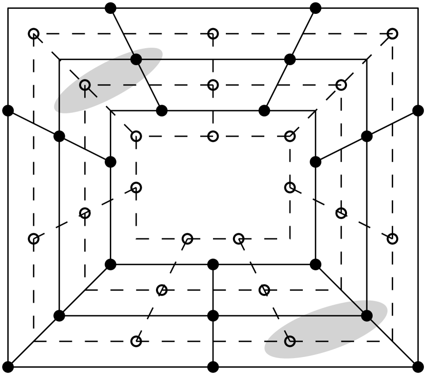
(a)

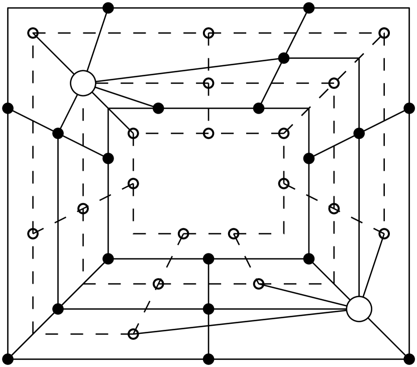
(b)

Figure 1: Theorem 1.2 does not hold for 1-plane graphs with $\times$-crossings.

Organization of the Paper:

In Section 2, we lay out the preliminaries, defining co-separating triples and $\Lambda(G)$ for 1-plane graphs. In Section 3, we generalize Theorem 1.1 to the class of full 1-plane graphs, which are 1-plane graphs where the endpoints of each crossing induce the complete graph $K_{4}$. Using this result we prove Theorem 1.2 in Section 4, and turn it into a linear-time algorithm in Section 5. We summarize in Section 6.

2 Preliminaries

We assume familiarity with graphs, see e.g. [7]. All graphs in this paper are assumed to be connected and have no loops. A separating set of a graph $G$ is a set $S$ of vertices such that $G\setminus S$ is disconnected; we use the term flap for a connected component of $G\setminus S$. Set $S$ separates two sets $A,B$ if there is no path connecting $A$ and $B$ in $G\setminus S$. The vertex connectivity of $G$, denoted $\kappa(G)$, is the cardinality of a minimum separating set. For any vertex set $A$, an $A$-vertex is a vertex that belongs to $A$; we also write $G$-vertex for a vertex of $V(G)$.

A drawing of a graph in the plane is called good if edges are simple curves that intersect only if they properly cross or have a common endpoint, any two edges intersect at most once, and no three edges cross in a point. A 1-planar graph is a graph that has a good drawing in the plane where each edge is crossed at most once; such a drawing is called a 1-planar drawing and a graph with a given 1-planar drawing is called a 1-plane graph. Throughout the paper, we assume that we are given a 1-plane graph $G$.

Let $\{(u,v),(w,x)\}$ be a crossing in $G$, i.e., edges $(u,v)$ and $(w,x)$ cross each other. The vertices $\{u,v,w,x\}$ are called endpoints of the crossing; these are four distinct vertices since the drawing is good. Two endpoints are called consecutive if they are not the two ends of $(u,v)$ or $(w,x)$. We distinguish six types of crossings by whether consecutive endpoints are adjacent (see Figure 2). As in [9], we call a crossing full if $\{u,v,w,x\}$ induces $K_{4}$, and almost-full if $\{u,v,w,x\}$ induces $K_{4}$ minus one edge. We call it bowtie if $\{u,v,w,x\}$ induces a cycle, arrow if $\{u,v,w,x\}$ induces $K_{1,3}$ plus one edge, chair if $\{u,v,w,x\}$ induces a path of length three (the length of a path is its number of edges), and the crossing is an $\times$-crossing otherwise (no edges connecting consecutive endpoints of the crossing). For an almost-full crossing, there are exactly two consecutive non-adjacent endpoints; we call these the wing tips and the other two endpoints the spine-vertices. For an arrow crossing, depending on whether an endpoint is adjacent to zero or two of its consecutive endpoints, we call it the tail or tip; the other two endpoints are the base vertices.

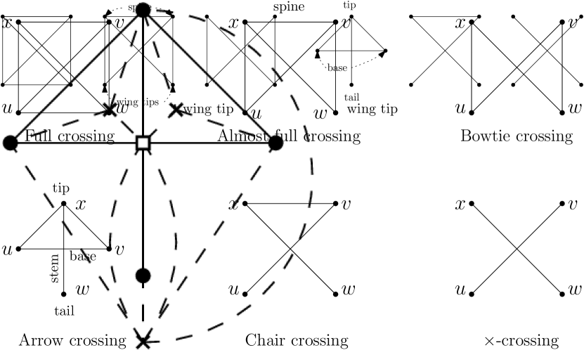
Figure 2: Types of crossings. From left to right: Full, almost-full, bowtie, arrow, chair and $\times$.

The planarization of $G$, denoted $G^{\times}$, is obtained by replacing any crossing $\{(u,v),(w,x)\}$ with a dummy vertex, i.e., remove the crossing edges and insert (at the point where the crossing used to be) a new vertex adjacent to all of $u,v,w,x$. The resulting drawing is planar, i.e., has no crossings. In a planar drawing $\Gamma$, a face is a maximal region of $\mathbb{R}^{2}\setminus\Gamma$. Drawing $\Gamma$ defines at each vertex $v$ the rotation $\rho(v)$, which is the circular list of incident edges and faces, ordered clockwise.

Pre-processing:

In Figure 2, we assumed that any edge $(u,x)$ between consecutive endpoints of a crossing is actually drawn near that crossing, i.e., $G^{\times}$ contains a face incident to $(u,x)$ and the dummy vertex of the crossing. (We call such a face a kite face and the edge a kite edge.) In general this may not be true. But if $(u,x)$ exists elsewhere in the drawing, then we can duplicate it and insert it as a kite edge. This affects neither 1-planarity nor vertex connectivity nor crossing type, so assume from now on that at any crossing all edges among consecutive endpoints exist as kite edges. Since we never create a face of $G^{\times}$ that is bounded by two edges, graph $G$ continues to have at most $4n-8$ edges.

Radial Planarization:

Recall that Eppstein [8] used the radialization to compute the vertex connectivity of a planar graph. We now generalize this concept to our 1-plane graph $G$ as follows. The radial planarization, denoted $\Lambda(G)$, is obtained by first planarizing $G$ to obtain $G^{\times}$, and then radializing $G^{\times}$ (see Figure 3). In other words, we add a face vertex $f$ inside each face $F$ of $G^{\times}$, and for every incidence of $F$ with a vertex $v$ we add an edge $(v,f)$, drawn inside $F$ and inserted in the drawing of $\Lambda(G)$ such that it bisects the occurrence of $F$ in the rotation $\rho(v)$. (Repeated incidences of $F$ with $v$ give rise to parallel edges $(f,v)$.) As in [10], we use the term radial graph for the subgraph $R(G)$ of $\Lambda(G)$ formed by the edges incident with face vertices. Note that $\Lambda(G)$ has three types of vertices: $G$-vertices, dummy vertices that replace crossings of $G$, and face vertices. For a cycle $C$ in $\Lambda(G)$, we define the shortcut $\mathbf{V}_{\!\!G}(C):=V(G)\cap V(C)$ for the $G$-vertices of $C$.

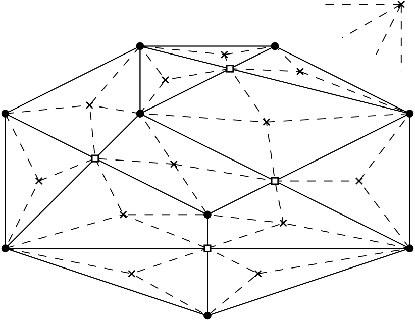
(a)

(b)

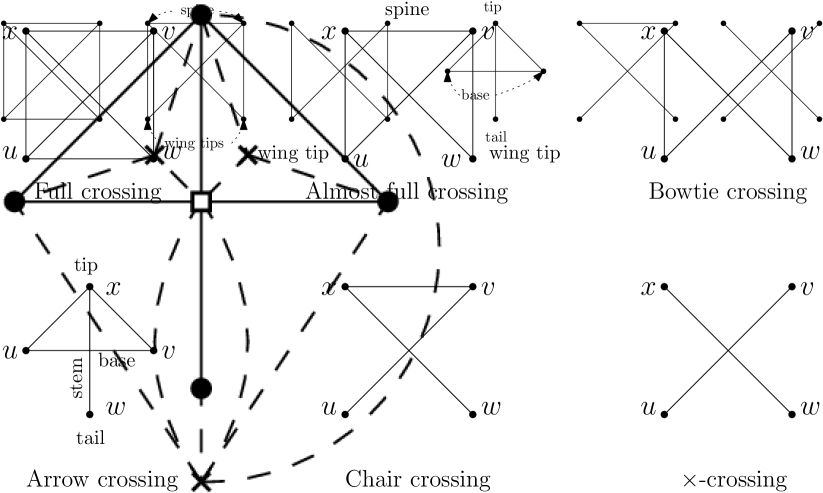
(c)

Figure 3: (a) A 1-plane graph $G$. (b) Its radial planarization $\Lambda(G)$. (c) $\Lambda(G)$ if $G$ is an arrow crossing. Face vertices are crosses, dummy vertices are white squares, edges of $R(G)$ are dashed.

Co-separating Triple:

We now clarify what it means to be separating in $G$ and $\Lambda(G)$ simultaneously. We will actually give this definition for an arbitrary graph $\Lambda$ that shares some vertices with $G$ (since it will later be needed for graphs derived from $\Lambda(G)$).

Definition 2.1 (Co-separating triple).

Let $\Lambda$ be a graph that shares some vertices with $G$. A partition of the vertices of $\Lambda$ into three sets $(A,X,B)$ is called a co-separating triple of $\Lambda$ if it satisfies the following properties:

1. Each of $A$, $X$ and $B$ contains at least one $G$-vertex.

2. For any two vertices $a\in A$ and $b\in B$, there is no edge $(a,b)$ in either $E(\Lambda)$ or $E(G)$.

We say that a co-separating triple of $\Lambda$ has diameter $d$ if any two vertices of $X$ have distance at most $d$ in $\Lambda$. When $\Lambda=\Lambda(G)$, then all $G$-vertices belong to $\Lambda$, and since $A$ and $B$ both contain $G$-vertices the following is immediate:

If $(A,X,B)$ is a co-separating triple of $\Lambda(G)$, then $X$ is a separating set of $\Lambda(G)$ and $X\cap V(G)$ is a separating set of $G$.

3 Full 1-Plane Graphs

In this section, we study full 1-plane graphs, i.e., 1-plane graphs where all crossings are full. In this case, we will find a co-separating triple $(A,X,B)$ that has a special form (this will be needed in Section 4): Vertex set $X$ contains no dummy vertices, forms a cycle $C$ in $R(G)$, and $A$ and $B$ are exactly the vertices inside and outside this cycle in the planar drawing of $\Lambda(G)$. (In other words, we generalize Theorem 1.1.)

Theorem 3.1.

Let $G$ be a full 1-plane graph and $S$ be a minimal separating set of $G$. Then there is a cycle $C$ in $R(G)$ such that $C$ does not visit dummy vertices, $\mathbf{V}_{\!\!G}(C)=S$, and there are vertices of $G$ inside and outside $C$.

Proof 3.2.

The broad idea is to take a maximal path in $R(G)$ that alternates between $S$-vertices and face vertices with suitable properties, and then close it up into a cycle $C$ of $R(G)$ that separates two vertices of $G$. Hence $C$ automatically does not visit dummy vertices and $\mathbf{V}_{\!\!G}(C)=S$ since $S$ is minimal. We explain the details now.

Call a face $F$ of $G^{\times}$ a transition face if $F$ is either incident to an edge between two $S$-vertices, or $F$ is incident to vertices from different flaps of $G\setminus S$. The corresponding face vertex in $\Lambda(G)$ is called a transition-face vertex. By walking along the boundary of a transition face, one can easily show the following (see the appendix):

Claim 1.

Every transition face $F$ contains at least two vertices of $S$ or two incidences with the same vertex of $S$.

In consequence, any transition-face vertex has (in $R(G)$) two edges to vertices of $S$. Vice versa, any $S$-vertex $v$ has (in $R(G)$) two transition-face neighbours, because in the planarization $G^{\times}$ we transition at $v$ from edges leading to one flap of $G\setminus S$ to edges leading to another flap and back; this can happen only at transition faces. See the appendix for a proof of the following claim (and for the formal definition of ‘clockwise between’).

Claim 2.

Let $(v,t_{1})$ and $(v,t_{2})$ be two edges of $G$ such that $v\in S$ and $t_{1}$ and $t_{2}$ are in different flaps of $G\setminus S$. Then there exists a transition face incident to $v$ that is clockwise between $(v,t_{1})$ and $(v,t_{2})$.

With this, it is obvious that we can find a simple cycle $C$ that alternates between transition-face vertices and $S$-vertices, but we need to ensure that $C$ has vertices of $G$ inside and outside, and for this, we choose $C$ more carefully. Formally, let $v_{1}$ be an arbitrary $S$-vertex. Let $P=v_{1}\dots v_{k}$ be a simple path that alternates between transition-face vertices and $S$-vertices and that is maximal in the following sense: $v_{k}\in S$, for any transition-face vertex $v_{k+1}$ adjacent to $v_{k}$ and any $S$-vertex $v_{k+2}$ adjacent to $v_{k+1}$, at least one of $v_{k+1},v_{k+2}$ already belongs to $P$. Since $v_{k}\in S$ and $S$ is minimal, $v_{k}$ has neighbours $t_{1},t_{2}$ in different flaps of $G\setminus S$. Applying Claim 2 twice gives a transition face $F$ clockwise between $(v_{k},t_{1})$ and $(v_{k},t_{2})$, and a transition face $F^{\prime}$ clockwise between $(v_{k},t_{2})$ and $(v_{k},t_{1})$. If $k>1$, then (up to renaming of $t_{1},t_{2},F^{\prime}$) we may assume that $v_{k-1}$ is the face vertex of $F^{\prime}$. Hence for $k>1$, edge $(v_{k},f)$ (where $f$ is the face vertex of $F$) is not on $P$, and the same holds vacuously also if $k=1$. We have cases:

(a)

(b)

(c)

Figure 4: Constructing the cycle $C$ (bold) in $R(G)$.

• In the first case, $f\in P$, say $f=v_{i}$ for some $1\leq i\leq k-1$ (Figure 4(a)). Then $C:=v_{i}v_{i+1}\dots v_{k}v_{i}$ is a cycle with $t_{1}$ and $t_{2}$ on opposite sides.

• In the second case $f\notin P$. By Claim 1, $R(G)$ contains at least two edges $e,e^{\prime}$ that connect $f$ to $S$-vertices. Up to renaming we may assume that $e=(v_{k},f)$. Consider extending $P$ via $e$ and $e^{\prime}$. By maximality of $P$ the result is non-simple, and by $f\notin P$ therefore $e^{\prime}=(f,v_{i})$ for some $1\leq i\leq k$.

  If $1\leq i\leq k-1$ (Figure 4(b)), then define simple cycle $C:=v_{i}v_{i+1}\dots v_{k}fv_{i}$ and observe that it has $t_{1}$ and $t_{2}$ on opposite sides. Otherwise ($i=k$) both edges $e,e^{\prime}$ connect $v_{k}$ to $f$ (Figure 4(c)), and we let $C$ be the cycle consisting of $e$ and $e^{\prime}$. There can be parallel edges incident to $f$ only because face $F$ of $G^{\times}$ was incident to $v_{k}$ repeatedly. Edges $e,e^{\prime}$ were then added to $\Lambda(G)$ in such a way that at least one other $G$-vertex on the boundary of $F$ lies between those incidences on either side of cycle $C$.

So in either case we have constructed a cycle $C$ in $R(G)$ with $\mathbf{V}_{\!\!G}(C)\subseteq S$ that does not visit dummy vertices and with two $G$-vertices (say $a$ and $b$) inside and outside $C$. To show that $\mathbf{V}_{\!\!G}(C)=S$, it is sufficient (by minimality of $S$) to show that $\mathbf{V}_{\!\!G}(C)$ is separating in $G$. To see this, fix any path $\pi$ from $a$ to $b$ in $G$ and let $\pi_{\Lambda}$ be the corresponding path in $\Lambda(G)$ obtained by replacing crossings by dummy vertices. Path $\pi_{\Lambda}$ must intersect $C$, but it uses only $G$-vertices and dummy vertices while $C$ uses only $G$-vertices and face vertices, so $\pi_{\Lambda}$ intersects $C$ in a vertex of $G$ and $\mathbf{V}_{\!\!G}(C)$ hence separates $a$ from $b$ in $G$.

4 1-Plane Graphs Without $\times$-Crossings

In this section, we prove Theorem 1.2: Minimal separating sets correspond to co-separating triples with small diameter. One direction is easy: If $\Lambda(G)$ has a co-separating triple $(A,X,B)$ with $|V(G)\cap X|\leq k$, then from Observation 2, $G$ has a separating set of size at most $k$.

Proving the other direction is harder, and we first give an outline. For the rest of this section, fix a minimal separating set $S$, and two arbitrary flaps $\phi_{1},\phi_{2}$ of $G\setminus S$. We first augment graph $G$ to $G_{\text{aug}}$ by adding more edges; this is done to reduce the types of crossings that can exist and thereby the number of cases. (Augmenting the graph is only used as a tool to prove Theorem 1.2; the vertex connectivity algorithm does not use it.) We then find a cycle $C$ for $\Lambda(G_{\text{aug}})$ with vertices of $G$ inside and outside $C$ such that all vertices of $S$ are in the neighbourhood of $C$. To do so we temporarily modify $G_{\text{aug}}$ further to make it a full 1-plane graph $G_{\text{aug}}^{+}$, appeal to Theorem 3.1, and show that the resulting cycle can be used for $C$. By setting $X_{\text{aug}}=V(C)\cup S$, this cycle gives a co-separating triple $(A_{\text{aug}},X_{\text{aug}},B_{\text{aug}})$ of $\Lambda(G_{\text{aug}})$, and using $C$ we can argue that the diameter of the graph induced by $X_{\text{aug}}$ is small. Finally we undo the edge-additions to transfer the co-separating triple from $\Lambda(G_{\text{aug}})$ to $\Lambda(G)$.

Augmentation:

We define the augmentation of $G$ with respect to $S,\phi_{1},\phi_{2}$ to be the graph $G_{\text{aug}}:=G_{\text{aug}}(S,\phi_{1},\phi_{2})$ obtained as the result of the following iterative process:

For any two consecutive endpoints $u,x$ of a crossing, if there is no kite edge $(u,x)$ and it could be added without connecting flaps $\phi_{1},\phi_{2}$, then add the kite edge, update the flaps $\phi_{1}$ and $\phi_{2}$ (because they may have grown by merging with other flaps), and repeat.

By construction $S$ remains a separating set with flaps $\phi_{1},\phi_{2}$ in $G_{\text{aug}}$, and it is minimal since adding edges cannot decrease connectivity. Also, one can easily show the following properties of crossings in $G_{\text{aug}}$ (here not having $\times$-crossings is crucial), see Figure 5 for an illustration, and the appendix for details.

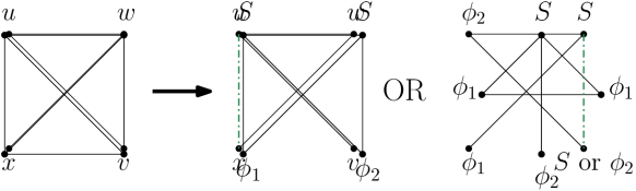
Figure 5: At a chair crossing, we can always add an edge to create an arrow-crossing.

The crossings of $G_{\textup{aug}}=G_{\textup{aug}}(S,\phi_{1},\phi_{2})$ have the following properties:

1. Any crossing is full, almost-full or an arrow crossing.

2. At any almost-full crossing, the spine vertices belong to $S$ and the wing tips belong to $\phi_{1}$ and $\phi_{2}$.

3. At any arrow crossing, the tip belongs to $S$, the tail belongs to one of $\phi_{1},\phi_{2}$, and the base vertices belong to the other of $\phi_{1},\phi_{2}$.

Extending Theorem 1.1?

Note that we expanded Theorem 1.1 (for plane graphs) to Theorem 3.1 (for full 1-plane graphs), but as we illustrate now, it cannot be expanded to 1-plane graphs without $\times$-crossings. One example for this is the graph that exists of exactly one arrow crossing (see Figure 3(c)), because the tip is a separating set, but there is no 2-cycle in $R(G)$ that contains the tip. For an example with higher connectivity, consider Figure 6. The figure shows a 1-plane graph where each crossing is an arrow crossing or a chair crossing. The graph is 4-connected and a minimum separating set $S$ is shown by vertices marked with white disks. One can verify that in the radial planarization of the graph, there is no 8-cycle in $R(G)$ that contains all vertices in $S$. (This example will also be used later as running example for our approach.)

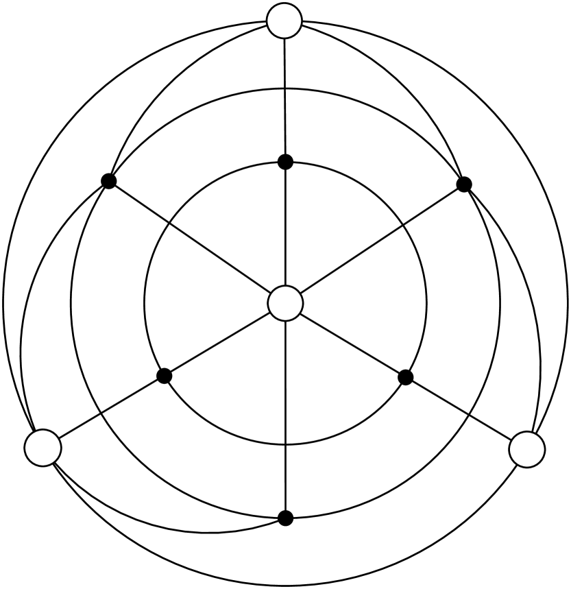
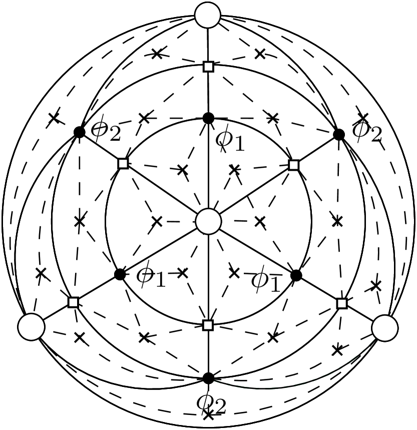
Figure 6: A 4-connected 1-plane graph $G$, its augmentation $G_{\text{aug}}$ with respect to the minimum separating set $S$ (white disks, the added edge is green/dot-dashed), and its radial planarization $\Lambda(G_{\text{aug}})$. Note that the unique chair crossing in $G$ becomes an arrow crossing in $G_{\text{aug}}$. The radial graph does not have an 8-cycle passing through $S$.

Cycle $C$ in $\Lambda(G_{\text{aug}})$:

So we cannot hope to find a cycle $C$ in $\Lambda(G_{\text{aug}})$ with $G$-vertices on both sides that goes exactly through $S$. But we can find a cycle $C$ that is “adjacent” to all of $S$. To make this formal, define for a cycle $C$ in $\Lambda(G_{\text{aug}})$ the set $\mathbf{V}_{\!\!\times}\!(C)$ to be the set of all vertices of $C$ that are vertices of $G_{\text{aug}}^{\times}$, i.e., they are $G$-vertices or dummy vertices of $\Lambda(G_{\text{aug}})$.

Lemma 4.1.

There is a cycle $C$ in $\Lambda(G_{\textup{aug}})$ that uses only edges of $R(G_{\textup{aug}}$) and such that

1. every vertex in $\mathbf{V}_{\!\!\times}\!(C)$ is either in $S$ or is a dummy vertex adjacent to an $S$-vertex,

2. every $S$-vertex is either in $\mathbf{V}_{\!\!\times}\!(C)$ or adjacent to a dummy vertex in $\mathbf{V}_{\!\!\times}\!(C)$,

3. there are $G$-vertices that are not in $S$ both inside and outside $C$, and

4. $S$ separates $G$-vertices inside $C$ from $G$-vertices outside $C$ in $G_{\textup{aug}}$.

Proof 4.2.

As outlined, we first convert $G_{\text{aug}}$ to a full 1-plane graph $G_{\text{aug}}^{+}$ as follows (see Figure 7 for the abstract construction and Figure 8(a) for the running example): At every almost-full crossing and every arrow crossing, replace the crossing with a dummy vertex. At every arrow crossing, furthermore add a base edge, which connects the base vertices and is inserted so that it forms a full crossing. Since every crossing of $G_{\text{aug}}$ is full, almost-full or arrow, all crossings of $G_{\text{aug}}^{+}$ are full. We use $D:=V(G_{\text{aug}}^{+})\setminus V(G)$ for the new vertices and note that every vertex in $D$ is adjacent to an $S$-vertex and corresponds to a dummy vertex in $\Lambda(G_{\text{aug}})$.

$\mathbf{\rightarrow}$

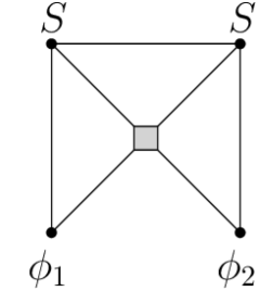
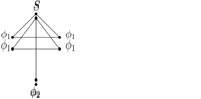
$\mathbf{\rightarrow}$

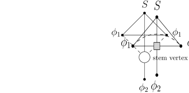
Figure 7: From $G_{\text{aug}}$ to $G_{\text{aug}}^{+}$. Vertices in $D$ are grey squares, the base edge is dashed.

Define $S^{+}:=S\cup D$ and observe that this is a separating set of $G_{\text{aug}}^{+}$ since no edge of $G_{\text{aug}}^{+}$ connects $\phi_{1}$ with $\phi_{2}$. Apply Theorem 3.1 to $G_{\text{aug}}^{+}$ and a subset of $S^{+}$ that is minimally separating. This gives a cycle $C$ in $R(G_{\text{aug}}^{+})$ such that $\mathbf{V}_{\!G_{\text{aug}}^{+}}\!\!(C)\subseteq S^{+}$, $C$ does not visit dummy vertices of $G_{\text{aug}}^{+}$, and there are $G_{\text{aug}}^{+}$-vertices inside and outside $C$. See Figure 8(b). We claim that $C$ satisfies all conditions, for which we first need to show that it actually is a cycle in $\Lambda(G_{\text{aug}})$. The only difference between $\Lambda(G_{\text{aug}})$ and $\Lambda(G_{\text{aug}}^{+})$ is at each base edge: Here $\Lambda(G_{\text{aug}}^{+})$ has an extra vertex $c$ (the dummy vertex for the crossing created by the base edge) and the four incident face vertices, while $\Lambda(G_{\text{aug}})$ has only the two face vertices of the kite faces at the arrow crossing. But by Theorem 3.1 cycle $C$ does not visit $c$, so $C$ also is a cycle of $\Lambda(G_{\text{aug}})$.

To see that $C$ satisfies (1), observe that $\mathbf{V}_{\!\!\times}\!(C)=\mathbf{V}_{\!G_{\text{aug}}^{+}}\!\!(C)\subseteq S^{+}=S\cup D$, and every vertex of $D$ is a dummy vertex of $\Lambda(G_{\text{aug}})$ that is adjacent to an $S$-vertex. Next we show (3). We know that there exist two vertices $a,b\in V(G_{\text{aug}}^{+})$ inside and outside $C$. If $a\in S\cup D$, then inspection of Figure 7 shows that $a$ has a neighbour $a^{\prime}$ in $\phi_{1}\cup\phi_{2}$ (hence $a^{\prime}\in V(G)$ but $a^{\prime}\not\in S\cup D$). By $\mathbf{V}_{\!\!\times}\!(C)\subseteq S\cup D$ therefore $a^{\prime}$ is on the same side of $C$ as $a$. Up to renaming hence $a\notin S\cup D$, and likewise $b\notin S\cup D$. This proves (3).

Before proving (2) and (4), we first show that the same vertices $a$ and $b$ are separated (in $G_{\text{aug}}$) by the set $S^{\prime}$ consisting of all $S$-vertices that are in $\mathbf{V}_{\!\!\times}\!(C)$ or adjacent to $\mathbf{V}_{\!\!\times}\!(C)\cap D$. To do so, pick an arbitrary path $\pi$ from $a$ to $b$ in $G_{\text{aug}}$. We define a path $\pi^{+}$ in $G_{\text{aug}}^{+}$ that corresponds to $\pi$ as follows: use the same set of edges of $\pi$, except if $\pi$ used an edge $(r,s)$ that is part of an almost-full or an arrow crossing. At an almost-full crossing, we replace $(r,s)$ by a path $r$-$d$-$s$ where $d\in D$ is the dummy vertex. At an arrow crossing we have two cases. If $r,s$ were the base vertices, then we replace $(r,s)$ by the base edge. If $r,s$ were tip and tail, then we replace $(r,s)$ by $r$-$d$-$s$ where $d\in D$ is the dummy vertex.

Since $\pi^{+}$ is a path from inside $C$ to outside $C$ in $G_{\text{aug}}$, it contains a vertex $w\in\mathbf{V}_{\!\!\times}\!(C)\allowbreak\subseteq S\cup D$. If $w\in S$, then define $t:=w$. If $w\in D$, then near $w$ path $\pi^{+}$ must have had the form $r$-$w$-$s$ for some $(r,s)\in\pi$, due to our construction of $\pi^{+}$. Furthermore, $(r,s)$ either belongs to an almost-full crossing, or to an arrow crossing with $(r,s)$ connecting the tip and tail. For both types of crossings, one of $r,s$ belongs to $S$, and we define $t$ to be this vertex. So we have found a vertex $t\in S$ on $\pi$ that is either on $\mathbf{V}_{\!\!\times}\!(C)$ or adjacent to a dummy vertex $d\in D\cap\mathbf{V}_{\!\!\times}\!(C)$. Therefore $t\in S^{\prime}$ and so any path from $a$ to $b$ intersects $S^{\prime}$. So $S^{\prime}\subseteq S$ is a separating set of $G_{\text{aug}}$, hence by minimality $S^{\prime}=S$, which proves (2). Also the $G$-vertices $a$ and $b$ are inside and outside $C$ and separated by $S$, which proves (4).

Notice that this lemma immediately implies a co-separating triple $(A_{\text{aug}},X_{\text{aug}},B_{\text{aug}})$ of $G_{\text{aug}}$: Fix such a cycle $C$, let $X_{\text{aug}}=V(C)\cup S$ and let $A_{\text{aug}}$ and $B_{\text{aug}}$ be the sets of vertices of $\Lambda(G_{\text{aug}})\setminus X_{\text{aug}}$ inside and outside $C$ respectively. See Figure 8(c). Clearly this is a partition, and by Lemma 4.1(3), both $A_{\text{aug}}$ and $B_{\text{aug}}$ have a $G$-vertex. As $A_{\text{aug}}$ and $B_{\text{aug}}$ are on opposite sides of cycle $C$, $V(C)\subseteq X_{\text{aug}}$ separates $A_{\text{aug}}$ and $B_{\text{aug}}$ in $\Lambda(G_{\text{aug}})$, and by Lemma 4.1(4), $S\subseteq X_{\text{aug}}$ separates $A_{\text{aug}}\cap V(G)$ and $B_{\text{aug}}\cap V(G)$ in $G_{\text{aug}}$. Therefore there can be no edge $(a,b)$ with $a\in A_{\text{aug}}$ and $b\in B_{\text{aug}}$ in either $\Lambda(G_{\text{aug}})$ or $G_{\text{aug}}$.

(a)

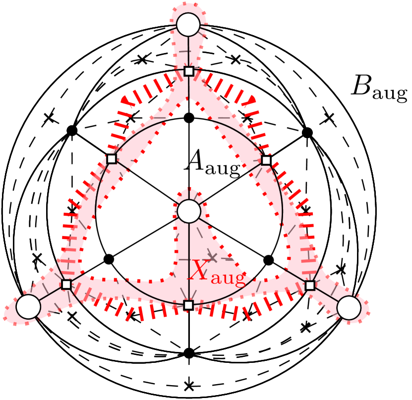
(b)

(c)

Figure 8: Finding a co-separating triple for the graph $G$ from Figure 6. (a) Graph $G_{\text{aug}}^{+}$; vertices in $D$ are grey squares and base edges are dashed. (b) Cycle $C$ for the minimal cutting set $D$; we do not show the face-vertices. Note that every vertex of $S$ is adjacent (in $G_{\text{aug}}$) to a dummy-vertex on $C$. (c) The resulting co-separating triples $(A_{\text{aug}},X_{\text{aug}},B_{\text{aug}})$.

Small Diameter:

In order to prove Theorem 1.2, we first argue that the subgraph of $\Lambda(G_{\text{aug}})$ induced by $X_{\text{aug}}$ has small diameter. Clearly the diameter of this graph is in $O(|C|)$ since all vertices of $X_{\text{aug}}$ are on $C$ or adjacent to it by Lemma 4.1(2). However, $|C|$ may not be in $O(|S|)$, which is why we need a more careful analysis to bound the length of a walk connecting two vertices of $X_{\text{aug}}$. Furthermore, to transfer the diameter-bound to $\Lambda(G)$ later, we need to exclude the edges that were added in $G_{\text{aug}}$ from such walks. Write $E_{\text{aug}}:=E(G_{\text{aug}})\setminus E(G)$ (in Figure 6 the unique edge in $E_{\text{aug}}$ is green/dash-dotted). Recall that edges in $E_{\text{aug}}$ are kite edges, hence connect two vertices of $G$ and have no crossing, therefore these edges also exist in $\Lambda(G_{\text{aug}})$.

Lemma 4.3.

For any two vertices $u,v\in X_{\text{aug}}$, there is a walk $W$ from $u$ to $v$ in $\Lambda(G_{\textup{aug}})$ that has length at most $4|S|$ and does not use edges of $E_{\text{aug}}$.

Proof 4.4.

Since $u,v\in X_{\text{aug}}$, they are either in $\mathbf{V}_{\!\!\times}\!(C)$ (recall that this includes dummy vertices of $\Lambda(G_{\text{aug}})$ on $C$), or face vertices on $C$, or in $S$. In the latter two cases they are within distance one of some vertex in $\mathbf{V}_{\!\!\times}\!(C)$. So there exist vertices $u^{\prime},v^{\prime}\in\mathbf{V}_{\!\!\times}\!(C)$ that are within distance at most one of $u$ and $v$, respectively. Enumerate one of the paths between $u^{\prime},v^{\prime}$ along cycle $C$ as $x_{0},\dots,x_{2t}$ with $x_{0}=u^{\prime}$ and $x_{2t}=v^{\prime}$. (Observe that the vertices in $\mathbf{V}_{\!\!\times}\!(C)$ are exactly the even-indexed ones since $C$ uses edges of $R(G_{\text{aug}})$.) Each vertex $x_{2i}$ for $i=0,\dots,t$ is either in $S$ (then set $s_{2i}:=x_{2i}$), or by Lemma 4.1(1) it is a dummy vertex that has a neighbour $s_{2i}\in S$. Define $\pi$ to be the walk

$$u,u^{\prime}{=}x_{0},s_{0},x_{0},x_{1},x_{2},s_{2},x_{2},x_{3},\dots,x_{2i-1},x_{2i},s_{2i},x_{2i},x_{2i+1},\dots,s_{2t},x_{2t}{=}v^{\prime},v,$$

i.e., it is the walk from $u$ to $v$ via $C$ with detours at even-indexed vertices to reach an $S$-vertex. Observe that $\pi$ has two properties: (1) At most three consecutive vertices in $\pi$ do not belong to $S$, and at the ends there are at most two consecutive vertices not in $S$; (2) if $y,z$ are two consecutive vertices of $\pi$ that are different, then at least one of them is a face vertex or a dummy vertex, hence $(y,z)\not\in E_{\text{aug}}$. We call a walk that satisfies (1) and (2) an $S$-hopping walk.

Let $W$ be the shortest $S$-hopping walk from $u$ to $v$. Observe that $W$ can visit any $S$-vertex at most once, for otherwise we could find a shorter $S$-hopping walk by omitting the part between a repeated $S$-vertex. Since $W$ contains at most three vertices between any two $S$-vertices, and at most two vertices not in $S$ at the beginning and end, it has length at most $4|S|$.

From $G_{\text{aug}}$ to $G$:

We now show how to transform $(A_{\text{aug}},X_{\text{aug}},B_{\text{aug}})$ into a co-separating triple $(A,X,B)$ of $\Lambda(G)$ of small diameter. Recall that $G_{\text{aug}}=G\cup E_{\text{aug}}$, so $\Lambda(G_{\text{aug}})$ is obtained from $\Lambda(G)$ by inserting the edges $E_{\text{aug}}$ and splitting any face vertex of a face that was divided by an edge in $E_{\text{aug}}$. We undo this in two parts. First, remove the edges of $E_{\text{aug}}$ from $\Lambda(G_{\text{aug}})$. This does not affect the separation properties of $(A_{\text{aug}},X_{\text{aug}},B_{\text{aug}})$ since we only remove edges, and it maintains the diameter since the walks of Lemma 4.3 do not use $E_{\text{aug}}$. The second step is to identify face vertices that belong to the same face of $G$. Define sets $A,B,X$ to be the same as $A_{\text{aug}},B_{\text{aug}},X_{\text{aug}}$ except that face vertices that were identified need to be replaced. To do so, observe that $A_{\text{aug}}$ and $B_{\text{aug}}$ are on opposite sides of $C$, and so no face vertex of $A_{\text{aug}}$ can get identified with a face vertex of $B_{\text{aug}}$ unless they both get identified with a face vertex of $C$. Thus the resulting face vertices come in three kinds: entirely composed of face vertices of $A_{\text{aug}}$ (add these to $A$), entirely composed of face vertices of $B_{\text{aug}}$ (add these to $B$), and containing a face vertex of $C$ (add these to $X$).

Clearly $A,B,X$ contain vertices of $G$ since $A_{\text{aug}},B_{\text{aug}},X_{\text{aug}}$ did and we only identified face vertices. Assume for contradiction that $(a,b)$ is an edge of $G$ or $\Lambda(G)$ for some $a\in A$ and $b\in B$. Then $(a,b)$ is not an edge in $G_{\text{aug}}$ or $\Lambda(G_{\text{aug}})$. Thus at least one of $a,b$ must be a face vertex that resulted from identifications. But with our choice of $A$ and $B$ then there was some edge $(a^{\prime},b^{\prime})$ in $\Lambda(G_{\text{aug}})$ connecting vertices in $A_{\text{aug}}$ and $B_{\text{aug}}$, a contradiction. Thus $(A,X,B)$ is the desired co-separating triple and Theorem 1.2 holds.

5 Computing Vertex Connectivity in Linear Time

In this section, we show how to use Theorem 1.2 to obtain a linear time algorithm for finding the vertex connectivity of 1-plane graphs without $\times$-crossings. The crucial insight is that we only need to find the smallest $k$ for which there is a co-separating triple $(A,X,B)$ with $|X\cap V(G)|=k$. Moreover, the subgraph of $\Lambda(G)$ induced by $X$ has small diameter. Therefore we can create some subgraphs $\Lambda_{1},\Lambda_{2},\dots$ of $\Lambda(G)$ that have small treewidth and $X$ belongs to at least one subgraph. (We assume that the reader is familiar with treewidth and its implications for algorithms; see for example [3] or the appendix.) We can search for a co-separating triple within these subgraphs using standard approaches for graphs of bounded treewidth, quite similar to the planar subgraph isomorphism algorithm by Eppstein [8].

The Graphs $\Lambda_{i}$:

As a first step, we perform a breadth-first search in $\Lambda(G)$ starting at an arbitrary vertex (the root); let $T$ be the resulting BFS-tree. For $j=1,2,\dots$ let $V_{j}$ (the $j$th layer) be the vertices at distance $j{-}1$ from the root, and let $d$ be the largest index where $V_{j}$ is non-empty. Define $V_{j}:=\emptyset$ for any index $j<1$ or $j>d$. For any $a\leq b$, the notation $\Lambda[V_{a}\cup\dots\cup V_{b}]$ will be a shortcut for the subgraph of $\Lambda(G)$ induced by $V_{a}\cup\dots\cup V_{b}$.

Assume that we know the size $k\leq 7$ of the separating set that we seek (we will simply try all possibilities for $k$ later). Define $w=4k+2\leq 30$, so we know that any two vertices in $X$ (of some putative co-separating triple $(A,X,B)$ that satisfies the conclusion of Theorem 1.2) have distance at most $w-2$ in $\Lambda(G)$. Hence $X$ belongs to $V_{i+1}{\cup}\dots\cup V_{i+w-2}$ for some $i\in\{0,\dots,d{-}w{+}2\}$. Thus we will search for $X$ within $\Lambda[V_{i+1}{\cup}\dots\cup V_{i+w-2}]$, but to guarantee that there are vertices representing $A$ and $B$ we also keep two extra layers above and below (i.e., layers $V_{i-1},V_{i},V_{i+w-1},V_{i+w}$). Furthermore, we add an edge set $U_{i-1}$ (‘upper edges’) within $V_{i-1}$ and an edge set $L_{i+w}$ (‘lower edges’) within $V_{i+w}$ that have some special properties.

Claim 3.

For $i\in\{0,\dots,d{-}w{+}2\}$, there exist sets of edges $U_{i-1}$ (connecting vertices of $V_{i-1}$) and $L_{i+w}$ (connecting vertices of $V_{i+w}$) such that the following holds:

1. Two vertices $u,v\in V_{i-1}$ can be connected via edges of $U_{i-1}$ if and only if there exists a path in $\Lambda[V_{1}\cup\dots\cup V_{i-1}]$ that connects $u$ and $v$.

2. Two vertices $u,v\in V_{i+w}$ can be connected via edges of $L_{i+w}$ if and only if there exists a path in $\Lambda[V_{i+w}\cup\dots\cup V_{d}]$ that connects $u$ and $v$.

3. The graph $\Lambda_{i}:=\Lambda[V_{i-1}{\cup}\dots\cup V_{i+w}]{\cup}U_{i-1}{\cup}L_{i+w}$ is planar and has radius at most $w{+}2$.

Furthermore, $\sum_{j=0}^{d-w+2}|U_{j}|{+}|L_{j}|\in O(n)$ and we can compute these sets in time $O(n)$.

Proof 5.1.

For $U_{i-1}$, this is easy. If $i=0,1$ then $V_{i-1}$ is empty and $U_{-1}=\emptyset$ works. Otherwise, pick an arbitrary vertex $r_{i-1}$ in $V_{i-1}$, and let $U_{i-1}$ be the edges that connect $r_{i-1}$ to all other vertices of $V_{i-1}$. In consequence, all vertices of $V_{i-1}$ can be connected within $U_{i-1}$, but this is appropriate since they can all be connected within the BFS-tree $T$, using only layers $1,\dots,i-1$ of $T$. Graph $\Lambda[V_{i-1}\cup\dots\cup V_{i+w}]\cup U_{i-1}$ is planar, because it can be obtained from the planar graph $\Lambda[V_{1}\cup\dots\cup V_{i+w}]$ by first contracting every vertex in layers $2,\dots,i-2$ into its parent in $T$ (yielding one super-node at the root), and then contracting this super-node into $r_{i-1}$.

For $L_{i+w}$, existence likewise is easy (and was argued by Eppstein [8]): Simply contract any edge of $\Lambda[V_{i+w}\cup\dots\cup V_{d}]$ that has at least one endpoint not in $V_{i+w}$, and let $L_{i+w}$ be the edges within $V_{i+w}$ that remain at the end. However, it is not obvious how one could implement contraction in overall linear time; we give an alternate approach for this in the appendix.

Since both $U_{i-1}$ and $L_{i+w}$ can be seen as obtained via contractions, graph $\Lambda_{i}$ is planar. To prove the radius-bound, define $r$ to be $r_{i-1}$ if $i\geq 2$ and to be the root of $T$ otherwise. Any vertex $v\in\Lambda_{i}$ has distance at most $w{+}2$ from $r$, because we can go upward from $v$ in $T$ at most $w{+}1$ times until we either reach a vertex $v$ in $V_{i-1}$ (which is $r{=}r_{i-1}$ or adjacent to it due to $U_{i-1}$), or $i\in\{0,1\}$ and we reach the root of $T$ (which is $r$).

An example of graph $\Lambda_{i}$ is given in the appendix.

Co-separating Triples in $\Lambda_{i}$.

We continue to assume that we know $k\leq 7$ (and hence $w=4k+2\leq 30$). Crucial for the correctness of our search for a co-separating triple in $\Lambda(G)$ is that it suffices to search in $\Lambda_{i}$ for all $i$.

Lemma 5.2.

There exists a co-separating triple $(A,X,B)$ of $\Lambda(G)$ with diameter $k$ if and only if there exists an index $i\in\{0,\dots,w{-}d{+}2\}$ and a co-separating triple $(A_{i},X,B_{i})$ of $\Lambda_{i}$ with diameter $k$ for which $X\subseteq\Lambda[V_{i+1}\cup\dots\cup V_{i+w-2}]$.

Proof 5.3.

Let $(A,X,B)$ be a co-separating triple of $\Lambda(G)$. Since $X$ has diameter at most $w-2$, all vertices of $X$ lie in the layers $i+1,\dots,i+w-2$ for some index $i$. Let $A_{i}$ and $B_{i}$ be subsets of $A$ and $B$ restricted to the vertices of $\Lambda_{i}$. We now show that $(A_{i},X,B_{i})$ is a co-separating triple of $\Lambda_{i}$. Clearly these sets partition $\Lambda_{i}$. Condition 1 (‘each set contains a $G$-vertex’) clearly holds for $X$. To see that it holds for $A_{i}$, consider graph $G$ in which $X\cap V(G)$ separates non-empty sets $A\cap V(G)$ and $B\cap V(G)$. Since $G$ is connected, there exists an edge $(a,x)$ with $a\in A\cap V(G)$ and $x\in X\cap V(G)$. This edge may or may not exist in $\Lambda(G)$, but if it does not then it got replaced by $a$-$c$-$x$ with a dummy vertex $c$. So $a$ has distance at most two from a vertex in $V_{i+1}\cup\dots\cup V_{i+w-2}$ and hence belongs to $V_{i-1}\cup\dots\cup V_{i+w}$, and so to $\Lambda_{i}$ and to $A_{i}$. The argument is symmetric for $B_{i}$.

Now we argue Condition 2 (‘no edges between $A_{i}$ and $B_{i}$ in $\Lambda_{i}$ or $G$’). Fix two vertices $a\in A_{i}$ and $b\in B_{i}$. Since $A_{i}\subseteq A$ and $B_{i}\subseteq B$, there is no edge $(a,b)$ in either $\Lambda(G)$ or $G$. So we are done unless $(a,b)$ is an edge of $U_{i-1}$ or $L_{i+w}$. Assume $(a,b)\in L_{i+w}$, the other case is similar. By Claim 3(2), there exists a path $\pi$ in $\Lambda[V_{i+w}\cup\dots\cup V_{d}]$ connecting $a$ and $b$. No vertex of $\pi$ belongs to $X$, and so the vertices of $\pi$ either all belong to $A$ or all belong to $B$ since $(A,X,B)$ is co-separating. This contradicts $a\in A$ and $b\in B$.

We now prove the other direction. Let $(A_{i},X,B_{i})$ be a co-separating triple of some $\Lambda_{i}$ with $X\subseteq\Lambda[V_{i+1}\cup\dots\cup V_{i+w-2}]$. We define $A$ and $B$ as follows. Begin with all vertices in $A_{i}$ and $B_{i}$, respectively; with this all vertices in $\Lambda_{i}$ belong to one of $A,X,B$. Now consider any vertex $v$ that does not belong to $\Lambda_{i}$, so either $v\in V_{1}\cup\dots\cup V_{i-2}$ or $v\in V_{i+w+1}\cup\dots\cup V_{d}$. Assume the latter (the other case is similar), and let $K$ be the component of $\Lambda[V_{i+w}\cup\dots\cup V_{d}]$ that contains $v$. By Claim 3(2), there exists a component $K^{\prime}$ of graph $(V_{i+w},L_{i+w})$ that contains exactly the vertices of $K\cap V_{i+w}$. The vertices of $K^{\prime}$ must either all be in $A_{i}$, or they must all be in $B_{i}$, because they are in layer $V_{i+w}$ (so not in $X$) and they are connected via $L_{i+w}$. Assign $v$ (and actually all vertices of $K$) to $A$ if $V(K^{\prime})\subseteq A_{i}$, and to $B$ otherwise.

We now show that partition $(A,X,B)$ is a co-separating triple of $\Lambda(G)$. Clearly Condition 1 holds since already $A_{i}$ and $B_{i}$ contain $G$-vertices. To show Condition 2, consider two vertices $a\in A$ and $b\in B$ and assume for contradiction that there is an edge $(a,b)$ in either $G$ or $\Lambda(G)$. This means that at least one of $a,b$ is not in $V_{i-1}\cup\dots\cup V_{i+w}$, else edge $(a,b)$ would contradict that $(A_{i},X,B_{i})$ was co-separating in $\Lambda_{i}$. Say $a\in V_{i+w+1}\cup\dots\cup V_{d}$, all other cases are similar. With this it is impossible that $(a,b)$ is an edge of $\Lambda(G)$: Such an edge would put $a,b$ into the same component of $\Lambda[V_{i+w}\cup\dots\cup V_{d}]$, but by construction of $A$ and $B$ we know that all vertices of such a component are put into the same set of $A$ and $B$.

So $(a,b)$ must be an edge of $G\setminus\Lambda(G)$, which means that it is crossed. Let $c$ be the dummy vertex on $(a,b)$. If $c\in A$ then $(c,b)$ is an edge of $\Lambda(G)$ with endpoints in $A$ and $B$, which we proved impossible already. Likewise $c\in B$ is impossible, so we must have $c\in X$. But then $c\in V_{i+1}\cup\dots\cup V_{i+w-2}$, which puts its neighbour $a$ into $V_{i}\cup\dots\cup V_{i+w-1}$, a contradiction.

Subroutine (To Find a Separating Set of Size $k$):

We continue to assume that we know $k\leq 7$ (and hence $w=4k+2\leq 30$). We also assume that edge-sets $U_{j}$ and $L_{j}$ have been computed already for all possible indices $j$, and that the edges of $\Lambda(G)$ have been split into $2d+1$ sets $E_{0},E_{0,1},\dots,E_{d-1,d},E_{d}$ where $E_{j}$ (for $j=0,\dots,d$) are all edges within layer $V_{j}$ while $E_{j-1,j}$ (for $j=1,\dots,d$) are all edges connecting $V_{j}$ to $V_{j+1}$. Perform the following for $i=0,\dots,d{-}w{+}2$:

1. Compute $\Lambda_{i}$. This takes time $O(|E(\Lambda_{i})|)$ time: The vertices are $V_{i-1}\cup\dots\cup V_{i+w}$, the edges are $U_{i-1}\cup E_{i-1,i}\cup E_{i}\cup\dots\cup E_{i+w-1,i+w}\cup L_{i+w}$, and all these sets are pre-computed.

2. Since $\Lambda_{i}$ is a planar graph with radius at most $w+2$, it has treewidth $O(w)$ [8] and a corresponding tree decomposition ${\cal T}$ can be found in $O(|E(\Lambda_{i})|)$ time. We may also assume that ${\cal T}$ has $O(|\Lambda_{i}|)$ bags.

3. We want to express Condition 2 of a co-separating triple as a condition in a single graph, and so define $\Lambda_{i}^{+}$ as follows: Begin with graph $\Lambda_{i}$, and add to it any edge $(v,w)$ of $G$ that is crossed (so is replaced in $\Lambda(G)$ by a path $v$-$c$-$w$ via dummy vertex $c$) and for which $v,w,c$ all belong to $\Lambda_{i}$.

4. Create a tree decomposition ${\cal T}^{+}$ of $\Lambda_{i}^{+}$ as follows. Begin with $\mathcal{T}$. For any bag $Y$ and any dummy vertex $c\in Y$, add to $Y$ all neighbours of $c$ that belong to $\Lambda_{i}$. One can argue that this is a tree decomposition of $\Lambda_{i}^{+}$ of width $O(5w)=O(1)$, and can be computed in $O(|\mathcal{T}|)=O(|\Lambda_{i}|)$ time, see the appendix.

5. Test whether $\Lambda_{i}$ has a co-separating triple $(A,X,B)$ for which $X$ contains exactly $k$ vertices of $G$ and lies within $V_{i+1}\cup\dots\cup V_{i+w-2}$. One can show (see the appendix) that this can be expressed in monadic second-order logic, using graph $\Lambda_{i}^{+}$ for defining adjacencies. By Courcelle’s famous theorem [5], since $\Lambda_{i}^{+}$ has a tree decomposition of constant width, therefore the test can be done in $O(|\mathcal{T}^{+}|)=O(|\Lambda_{i}|)$ time.

6. If we find such a co-separating triple, then break (and output $X\cap V(G)$ as a separating set of size $k$), else try the next $i$.

The run-time for one index $i$ is hence $O(|E(\Lambda_{i})|)$. To bound the total run-time, we must bound $\sum_{i=0}^{d}|E(\Lambda_{i})|$. Since each $\Lambda_{i}$ uses $w+2$ consecutive layers, any edge of $\Lambda(G)$ belong to at most $w+2$ sets in $E(\Lambda_{0}),\dots,E(\Lambda_{d-w+1})$. Any edge in $U_{0},\dots,U_{d},L_{0},\dots,L_{d}$ belongs to exactly one set in $E(\Lambda_{0}),\dots,E(\Lambda_{d-w+1})$. Therefore $\sum_{i=0}^{d-w+1}|E(\Lambda_{i})|\leq(w+2)|E(\Lambda(G)|+\sum_{i=0}^{d-w+1}(|U_{i}|+|L_{i}|)\in O(w|E(\Lambda(G))|)+O(n)$, which by $w\in O(1)$ and $|E(\Lambda(G)|\in O(n)$ shows that the total run-time is linear.

The Final Algorithm:

The algorithm for testing vertex-connectivity hence proceeds as follows. First pre-process $G$ and duplicate edges to become kite edges where required. Then compute $\Lambda(G)$, the BFS-tree and the layers, and the edge-sets $E_{j},E_{j,j{+}1}$, $U_{j}$ and $L_{j}$ for $j=0,\dots,d{+}2$. All this takes $O(n)$ time since $\Lambda(G)$ has $O(n)$ edges. For $k=1,\dots,7$, run the sub-routine to test whether there exists a separating set of size $k$; this will necessarily find the minimum such set. Each such run takes time $O(n)$, and since there is a constant number of them the overall time is linear and Theorem 1.3 holds.

6 Outlook

In this paper, we showed that the vertex connectivity of a 1-plane graph $G$ without $\times$-crossings can be computed in linear time. The main insight is that the distance (in an auxiliary graph) between any two vertices of a minimum separating set of $G$ must be bounded. We close with some open questions. First, can we deal with $\times$-crossings?

Open problem 1.

Can the vertex connectivity of an arbitrary 1-plane graph be computed in linear time?

In our ‘bad example’ (Figure 1), all crossings were $\times$-crossings. As a first step towards Problem 1, could we at least compute the vertex connectivity in linear time if the number of $\times$-crossings is bounded by a constant?

Throughout the paper, we assumed that the input came with a fixed 1-planar embedding. We did this since testing 1-planarity is NP-hard [14]. However, it might be easier to test whether there exists a 1-planar embedding without $\times$-crossing; all the existing NP-hardness proofs of 1-planarity that we are aware of [14, 22, 1, 4] have $\times$-crossings in the 1-planar drawings.

Open problem 2.

Is it NP-hard to test whether a given graph has a 1-planar drawing without $\times$-crossing?

The crucial ingredient for our result was the structural property that vertices of a separating set are close in some sense. Are there similar structural properties for edge connectivity or bisections? Are there similar results for other classes of near-planar graphs?

Appendix

Appendix A Limitations Explored Further

We already argued that there are graphs with $\times$-crossings for which the two vertices of the unique minimum separating set are arbitrarily far apart (Figure 1). These graphs are only 2-connected, and therefore not really an obstacle to a linear-time algorithm for testing vertex connectivity, since 3-connectivity can be tested in linear time by different means. We tried to generalize this counter-example to 1-plane graphs with higher connectivity, but failed thus far for 1-planar graphs. It is possible to achieve higher connectivity if we allow up to two crossings in each edge; see Figure 9 for an example.

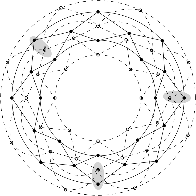
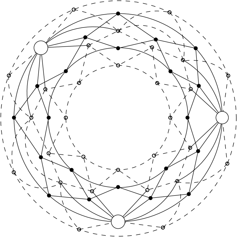
Figure 9: A graph drawn with at most two crossings per edge; both components are 4-connected. After fusing vertices in the grey shaded areas, they become the unique minimum separating set, and they could be made arbitrarily far apart in the radial planarization by adding more concentric layers and more vertices within layers.

Appendix B Missing Proofs of Section 3

B.1 Proof of Claim 1

We want to show that in a full 1-plane graph, every transition face $F$ contains at least two vertices of $S$ or two incidences with the same vertex of $S$.

Proof B.1.

This clearly holds if $F$ is incident to an edge $(s,s^{\prime})$ with $s,s^{\prime}\in S$, so assume that $F$ contains vertices $u\in\phi_{1}$ and $w\in\phi_{2}$ for two flaps $\phi_{1},\phi_{2}$ of $G\setminus S$. The clockwise walk along the boundary of $F$ from $u$ to $w$ must transition somewhere from vertices in $\phi_{1}$ to vertices in $\phi_{2}$. This transition cannot happen at a dummy vertex because $G$ is full 1-plane: Any face incident to a dummy vertex is a kite face, and its two vertices of $G$ are adjacent and hence not in different flaps. Therefore the transition to $\phi_{1}$ to $\phi_{2}$ happens at a vertex of $S$. A second such incidence can be found when we transition from $\phi_{2}$ to $\phi_{1}$ while walking in clockwise direction from $w$ to $u$ along the boundary of $F$.

B.2 Proof of Claim 2

We want to show that in a full 1-plane graph, at any vertex $v\in S$ and any two edges from $v$ to different flaps of $G\setminus S$, we can find a transition face that is clockwise between the edges.

We first define exactly what we mean by ‘clockwise between’. Consider the rotation $\rho(v)$ in the planar graph $G^{\times}$, i.e., the clockwise cyclic order of edges and faces incident to $v$. We can also define a rotation $\rho_{G}(v)$ for graph $G$, by replacing each edge $e$ in $\rho(v)$ by the corresponding edge $e^{\prime}$ in $G$ (if $e$ ended at a dummy vertex then $e^{\prime}$ is the entire crossed edge of $G$) and replacing each face $F$ in $\rho(v)$ by the corresponding cell (maximum region in the drawing of $G$). A cell may have crossings rather than dummy vertices on its boundary but is otherwise the same region of the drawing as the face. For any three elements $x,y,z$ of $\rho_{G}(v)$, we say that $y$ lies clockwise between $x$ and $z$ if $\rho_{G}(v)$ contains $x,y,z$ in this order (possibly with other elements in-between). The statement of the claim is hence that given two edges $(v,t_{1}),(v,t_{2})$ in $G$ where $t_{1},t_{2}$ are in different flaps, we can find a face $F$ incident to $v$ in $G^{\times}$ such that the corresponding cell lies between $(v,t_{1})$ and $(v,t_{2})$ in $\rho_{G}(v)$.

Proof B.2.

Scanning in $\rho_{G}(v)$ from $(v,t_{1})$ until $(v,t_{2})$, let $(v,w)$ be the last edge for which $w$ is in the same flap $\phi_{1}$ as $t_{1}$. Let the next few entries in $\rho_{G}(v)$ be $(v,w),F,(v,w^{\prime}),F^{\prime},(v,w^{\prime\prime})$ for cells $F,F^{\prime}$ and vertices $w^{\prime},w^{\prime\prime}$; we use $F,F^{\prime}$ also for the corresponding faces in $G^{\times}$. See Figure 10. We know $w^{\prime}\not\in\phi_{1}$ by choice of $w$ and have three cases.

Assume first that $(v,w^{\prime})$ is crossed. Since $G$ is full 1-plane, this crossing has four kite faces, and since these occur before/after the crossed edge in the rotation, $F,F^{\prime}$ must be kite faces of this crossing. Hence the edge that crosses $(v,w^{\prime})$ is $(w,w^{\prime\prime})$ and we have kite edges $(w,w^{\prime})$ and $(w^{\prime},w^{\prime\prime})$. Since $w\in\phi_{1}$ we have $w^{\prime}\in S\cup\phi_{1}$, but $w^{\prime}\not\in\phi_{1}$, so $w^{\prime}\in S$ and in particular $w^{\prime}\neq t_{2}$ (which is in $\phi_{2}$). Therefore $w^{\prime\prime}\not\in\phi_{1}$ by choice of $w$, and due to edge $(w,w^{\prime\prime})$ therefore $w^{\prime\prime}\in S$ as well. This makes $F^{\prime}$ incident to edge $(v,w^{\prime\prime})$ with both endpoints in $S$ and $F^{\prime}$ is a transition face.

Now assume that $(v,w)$ is crossed. This makes $F$ a kite face, hence $w^{\prime}$ is an endpoint of the crossing and kite edge $(w,w^{\prime})$ exists. As above therefore $w^{\prime}\in S$, and $F$ is incident to kite edge $(v,w^{\prime})$ with both endpoints in $S$. So $F$ is a transition face.

Finally assume that neither $(v,w^{\prime})$ nor $(v,w)$ have crossings, hence both $w^{\prime},w$ also belong to $F$. If $w^{\prime}\in S$ then $F$ is incident to edge $(v,w^{\prime})$ with both endpoints in $S$. If $w^{\prime}\not\in S$, then by $w^{\prime}\not\in\phi_{1}$ vertex $w^{\prime}$ belongs to a different flap than $w$. Either way $F$ is a transition face.

Figure 10: Finding the transition-face between $(v,t_{1})$ and $(v,t_{2})$.

Appendix C Missing Proofs of Section 4

Recall that $G_{\text{aug}}$ was obtained from $G$ (after fixing a minimum separating set $S$ and two flaps $\phi_{1},\phi_{2}$) by adding any kite edge that can be added while keeping $\phi_{1},\phi_{2}$ distinct flaps. We now discuss its properties.

The crossings of $G_{\textup{aug}}=G_{\textup{aug}}(S,\phi_{1},\phi_{2})$ have the following properties:

1. Any crossing is full, almost-full or an arrow crossing.

2. At any almost-full crossing, the spine vertices belong to $S$ and the wing tips belong to $\phi_{1}$ and $\phi_{2}$.

3. At any arrow crossing, the tip belongs to $S$, the tail belongs to one of $\phi_{1},\phi_{2}$, and the base vertices belong to the other of $\phi_{1},\phi_{2}$.

Proof C.1.

Consider an arbitrary crossing $\{(u,v),(w,x)\}$ of $G_{\text{aug}}$ that is not full, so there are two consecutive endpoints that are not adjacent. Since $G$ had no $\times$-crossing, there are two consecutive endpoints that are adjacent. Up to renaming we may hence assume that $(u,w)$ is a kite edge while $(u,x)$ does not exist. Since $(u,x)$ could not be added in $G_{\text{aug}}$, hence (up to renaming of flaps) $u\in\phi_{1}$ and $x\in\phi_{2}$. This implies $w\in S$ (since it is adjacent to both $u$ and $x$) and therefore kite edge $(w,v)$ can always be added. Due to edge $(u,v)$ we have $v\in S\cup\phi_{1}$. If $v\in S$ then edge $(x,v)$ can also be added; the crossing is then an almost-full crossing that satisfies (2). If $v\in\phi_{1}$ then $(x,v)$ cannot be added; the crossing is then an arrow crossing that satisfies (3).

Appendix D Missing Proofs for Section 5

We fill in here some details of claims made in Section 5.

D.1 The Graph $\Lambda_{i}$

See Figure 11 for an example of $\Lambda_{3}$.

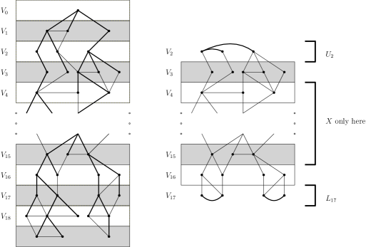
Figure 11: Construction of $\Lambda_{3}$ for $w=14$. Edges in $U_{2}$ and $L_{17}$ are bold.

D.2 Construction of $L_{j}$

Recall that we still need to explain how to find a set $L_{j}$ suitable for Claim 3 in linear time. We already argue that it exists via contractions. Performing such contractions blindly may, however, be too slow, since the resulting graph may not be simple and hence $|L_{j}|$ need not be in $O(|V_{j}|)$. We therefore explain here how to intersperse contractions with simplifications (elimination of parallel edges and loops) in such a way that the overall run-time is linear.

We construct $L_{j}$ in reverse order (i.e., for $j=d$ down to $0$) as follows. Set $L_{d}$ is simply $E_{d}$, the edges within layer $V_{d}$. To compute $L_{j}$ for $j<d$, we need the notation $p(v)$ for the parent of a vertex $v$ in the BFS-tree. We first compute a set $\hat{L}_{j}$ as follows:

• Add any edge $(v,w)$ of $E_{j}$ to $L_{j}$.

• For any edge $(v,w)$ of $E_{j,j+1}$ (say $v\in V_{j}$ and $w\in V_{j+1}$), add edge $(v,p(w))$ to $\hat{L}_{j}$.

• For any edge $(v,w)$ of $L_{j+1}$, add edge $(p(v),p(w))$ to $\hat{L}_{j}$.

Then we simplify, i.e., we parse the graph $(V_{j},\hat{L}_{j})$ to compute the underlying simple graph (this takes $O(|V_{j}|+|\hat{L}_{j}|)$ time), and let $L_{j}$ be the resulting edge-set.

Graph $(V_{j},L_{j})$ could have been obtained from $\Lambda[V_{j}\cup\dots\cup V_{d}]$ via a sequence of edge-contractions and simplifications.

Proof D.1.

Clearly this holds for $j=d$, so assume $j<d$. We can obtain graph $(V_{j},\hat{L}_{j})$ from $\Lambda[V_{j}\cup\dots\cup V_{d}]$ as follows. First perform all the edge-contractions and simplifications necessary to convert subgraph $\Lambda[V_{j+1}\cup\dots\cup V_{d}]$ into $(V_{j+1},L_{j+1})$; this is possible by induction. Now for as long as there is some vertex $w\in V_{j+1}$ left, contract $w$ into its parent $p(w)$. For any neighbour $v$ of $w$, edge $(v,w)$ hence gets replaced by $e^{\prime}=(v,p(w))$. We know $v\in V_{j}\cup V_{j+1}$ (all other vertices were eliminated via contractions already). If $v\in V_{j}$, then edge $e^{\prime}$ exists in $\hat{L}_{j}$. If $v\in V_{j+1}$, then at some point later we will contract $v$ into $p(v)$ and replace edge $e^{\prime}$ by $e^{\prime\prime}=(p(v),p(w))$; this edge exists in $\hat{L}_{j}$. So after the contractions we have a subgraph of $(V_{j},\hat{L}_{j})$. Vice versa, any of the three kinds of edges of $\hat{L}_{j}$ is obtained, since by induction the edges of $L_{j+1}$ were created. So we can create $(V_{j},\hat{L}_{j})$ with edge-contractions and simplifications, and get $(V_{j},L_{j})$ from it with further simplifications.

With this $L_{j}$ satisfies Claim 3(2) and 3(3) since planarity and connected components are not changed when doing edge-contractions and simplifications. It remains to analyze the run-time. Constructing $\hat{L}_{j}$ is proportional to the number of edges handled, since we do not contract but only have to look up parent-references $p(\cdot)$ which takes constant time. We handle at most $|E_{j}|+|E_{j,j+1}|$ edges of the first two type, and $|L_{j+1}|$ edges of the third type. Graph $(V_{j+1},L_{j+1})$ is planar and simple, so $|L_{j+1}|\in O(|V_{j+1}|)$. Summing over all $j$, the run-time is

$$O\big{(}\,\,\sum_{j=1}^{d}(|E_{j}|+|E_{j,j+1}|)+\sum_{j=0}^{d}|V_{j+1}|\,\,\big{)}=O\big{(}|E(\Lambda(G))|+|V(\Lambda(G))|\big{)}=O(n)$$

which also implies $\sum_{i=1}^{d}|L_{j}|\in O(n)$ since within this time we create all edges of all sets.

D.3 Treewidth and a Tree Decomposition of $\Lambda_{i}^{+}$

A tree decomposition of a graph $G$ is a tree $\mathcal{T}$ whose vertices (‘bags’) are subsets of $V(G)$ such that

• every vertex $v$ of $G$ is covered, i.e., $v$ belongs to at least one bag of $\mathcal{T}$,

• every edge $(u,v)$ of $G$ is covered, i.e., there exists a bag $Y\in V(\mathcal{T})$ with $u,v\in Y$, and

• for every vertex $v$ of $G$, the set $\mathcal{T}[v]$ of bags containing $v$ is contiguous, i.e., forms a connected subtree of $\mathcal{T}$.

The width of a tree decomposition is $\max_{Y\in V(\mathcal{T})}|Y|-1$, and the treewidth of a graph $G$ is the smallest width of a tree decomposition of $G$. We refer to [3] for an overview of the many algorithmic implications if a graph is known to have constant treewidth; in particular many NP-hard problems become polynomial. With this definition in place, we can argue the following:

Claim 4.

Let $\mathcal{T}$ be a tree decomposition of $\Lambda_{i}$ of width $O(w)=O(1)$. Let $\mathcal{T}^{+}$ be obtained by adding, for each bag $Y$ of $\mathcal{T}$ and each dummy vertex $c\in Y$, all neighbours of $c$ that are in $\Lambda_{i}$ to $Y$. Then $\mathcal{T}^{+}$ is a tree decomposition of $\Lambda_{i}^{+}$ that has width $O(5w)$ and that can be computed in time $O(|\mathcal{T}|)$.

Proof D.2.

The claim on the width and run-time is easy. Since dummy vertices have 4 neighbours in $\Lambda(G)$, we add at most 4 new vertices for each vertex in $Y$, so the width of $\mathcal{T}^{+}$ is at most $5|Y|$. Also, we spend constant time per vertex in $Y$, so $O(w)=O(1)$ time per bag, and the time to compute $\mathcal{T}^{+}$ is $O(|\mathcal{T}|)$.

For any vertex $v\in\Lambda_{i}$, the set $\mathcal{T}[v]$ of bags containing $v$ is contiguous. We must argue that $\mathcal{T}^{+}[v]$ is likewise contiguous. Vertex $v$ got added to more bags only if it was a neighbour of some dummy vertex $c$, and then it got added to all of $\mathcal{T}[c]$. Since there is an edge $(v,c)$ in $\Lambda_{i}$, there must be some bag in $\mathcal{T}[v]\cap\mathcal{T}[c]$, and so the new set of bags containing $v$ is again contiguous.

Finally for any edge $(u,v)$ in $\Lambda_{i}^{+}$, if $(u,v)\in\Lambda_{i}$ then it was already covered by $\mathcal{T}$. If $(u,v)\notin\Lambda_{i}$, then it was an edge of $G$ that was replaced by a path $u$-$c$-$v$ (for some dummy vertex $c$) in $\Lambda(G)$. We added $(u,v)$ to $\Lambda_{i}^{+}$ only if all of $u,c,v$ belong to $\Lambda_{i}$. So $c$ belongs to some bag $Y$ of $\mathcal{T}$, and we add $u,v$ to this bag $Y$, which means that edge $(u,v)$ is covered in $\mathcal{T}^{+}$.

D.4 Monadic Second-Order Logic

We claimed that testing whether $\Lambda_{i}$ has a suitable co-separating triple can be expressed using monadic second-order logic. To prove this, we first rephrase ‘being a suitable co-separating triple’ as a mapping into sets, then define monadic second-order logic, and then give the transformation.

Claim 5.

Graph $\Lambda_{i}$ has a co-separating triple $(A_{i},X,B_{i})$ with $|X\cap V(G)|=k$ and $X\subseteq V_{i+1}\cup\dots\cup V_{i+w+2}$ if and only if we can map the vertices of $\Lambda_{i}$ into sets $X_{1},\dots,X_{k},X_{\text{rest}},A,B$ that satisfy the following:

• Every vertex belongs to exactly one of the sets $X_{1},\dots,X_{k},X_{\text{rest}},A,B$.

• $X_{1},\dots,X_{k},X_{\text{rest}}$ contain only vertices in $V_{i+1}\cup\dots\cup V_{i+w-2}$.

• $X_{1},\dots,X_{k}$ contain exactly one vertex each, and that vertex belongs to $G$.

• $X_{\text{rest}}$ contains only dummy vertices and face vertices.

• $A,B$ contain at least one vertex that belongs to $G$.

• For any two vertices $a,b$, if $a\in A$ and $b\in B$ then there is no edge $(a,b)$ in $\Lambda_{i}^{+}$.

Proof D.3.

The mapping between the sets is the obvious one: $A_{i}$ corresponds to $A$, $B_{i}$ corresponds to $B$, $X_{j}$ (for $j=1,\dots,k$) corresponds to the $j$th $G$-vertex of $X$, and $X_{\text{rest}}$ are all vertices of $X$ that are not $G$-vertices. Given a co-separating triple $(A_{i},X,B_{i})$ of $\Lambda_{i}$, the conditions on the mapping are then easily verified since all edges of $\Lambda_{i}^{+}$ are also edges of $G$ or $\Lambda(G)$.

Vice versa, given a mapping into sets, we must verify that the corresponding triple $(A_{i},X,B_{i})$ is co-separating. The only non-trivial aspect here is Condition (2) of a co-separating triple, since $\Lambda_{i}^{+}$ does not contain all edges of $G$. So fix some $a\in A_{i}$ and $b\in B_{i}$, and assume for contradiction that $(a,b)$ is an edge in $\Lambda_{i}$ or $G$, but not an edge of $\Lambda_{i}^{+}$. Since $\Lambda_{i}$ is a subgraph of $\Lambda_{i}^{+}$, this means that $(a,b)$ is an edge of $G$ but not of $\Lambda_{i}$. Since $a,b$ are vertices of $\Lambda_{i}$, we would have added $(a,b)$ to $\Lambda_{i}^{+}$ unless $(a,b)$ was crossed in $G$, and the dummy vertex $c$ that replaced the crossing in $\Lambda(G)$ did not belong to $\Lambda_{i}$. (This may happen if $a,b\in V_{i-1}$ or $a,b\in V_{i+w}$ and $c$ belongs to the adjacent layer that is not in $\Lambda_{i}$.) Let us assume that $c$ belongs to $V_{i+w+1}\cup\dots\cup V_{d}$; the other case is symmetric. Then path $a$-$c$-$b$ connects $a$ and $b$ within layers $V_{i+w}\cup\dots\cup V_{d}$, and by Claim 3 therefore $a$ and $b$ are connected via a path $\pi$ that uses only edges of $L_{i+w}$; in particular none of the intermediate vertices of $\pi$ belong to $X$. Since $L_{i+w}$ belongs to $\Lambda_{i}$, hence to $\Lambda_{i}^{+}$, path $\pi$ also belongs to $\Lambda_{i}^{+}$. In consequence $a\in A$ and $b\in B$ is impossible, since otherwise somewhere along path $\pi$ we would transition from $A$-vertices to $B$-vertices at an edge of $\Lambda_{i}^{+}$.

We will not define the full concept of monadic second-order logic (see e.g. [6]), but only how it pertains to formulating graph decision problems. We assume that we are given some graph (in our application it is $\Lambda_{i}^{+}$ for some index $i$); its edge-set is expressed via a binary relation $E(x,y)$ that is true if and only if $(x,y)$ is an edge. We may also have a finite set of unary relations on the vertices; in our application we will need $V_{j}(x)$ that is true if and only if vertex $x$ belongs to layer $V_{j}$, and $V_{G}(x)$ that is true if and only if vertex $x$ belongs to $V(G)$. We want to find a logic formula of finite length that is true if and only if our graph decision problem has a positive answer. To express the logic formula, we are allowed to use quantifiers $\exists,\forall$ over vertex-sets, but not over edge-sets.

In our application, we want to know whether we can map the vertices of $\Lambda_{i}$ into sets $X_{1},\dots,X_{k},X_{\text{rest}},A,B$ that satisfy the conditions of Claim 5. We can express this in monadic second-order logic as follows: $\exists X_{1},\dots,X_{k},X_{\text{rest}},A,B\subseteq V(\Lambda_{i}):$

• $\forall x\bigwedge_{S\in\{X_{1},\dots,X_{k},X_{\text{rest}},A,B\}}x\in S$ (‘every vertex belongs to at least one set’), and

• $\forall x\bigwedge_{S\neq T\in\{X_{1},\dots,X_{k},X_{\text{rest}},A,B\}}x{\in}S{\Rightarrow}x{\notin}T$ (‘every vertex belongs to at most one set’), and

• $\forall x\bigwedge_{S\in\{X_{1},\dots,X_{k},X_{\text{rest}}\}}\bigwedge_{j\in\{i-1,i,i+w-1,i+w\}}x{\in}S{\Rightarrow}{\neg}V_{j}(x)$ (‘$X$ is not in outer layers’), and

• $\forall x,y\bigwedge_{j=1}^{k}(x\in X_{j}\wedge y\in X_{j}\Rightarrow x=y)$ (‘set $X_{j}$ contains at most one vertex’), and

• $\bigwedge_{j=1}^{k}\exists x:x\in X_{j}$ (‘each $X_{j}$ contains at least one vertex’), and

• $\forall x\bigwedge_{j=1}^{k}(x\in X_{j}\Rightarrow V_{G}(x))$ (‘each $X_{j}$ contains only $G$-vertices’), and

• $\forall x:x\in X_{\text{rest}}\Rightarrow\neg V_{G}(x)$ (‘set $X_{\text{rest}}$ contains no $G$-vertices’), and

• $\bigwedge_{S\in\{A,B\}}\exists x:x\in S\wedge V_{G}(x)$ (‘$A$ and $B$ contain at least one $G$-vertex’), and

• $\forall x,y:x\in A\wedge y\in B\Rightarrow\neg E(x,y)$ (‘no edge between $A$ and $B$’)

Since $k\leq 7$, this is a finite-length formula.

It should be mentioned here that monadic second-order logic is more powerful than really required to find a co-separating triple. It is not hard to show (but a bit tedious to describe) that one can test ‘does there exist a mapping as in Claim 5’ directly, using bottom-up dynamic programming in the tree decomposition of $\Lambda_{i}^{+}$. (This is also the reason why we gave the explicit construction of the tree decomposition in Claim 4, rather than only arguing that $\Lambda_{i}^{+}$ has bounded treewidth.) We leave the details to the reader.

References

- [1] Christopher Auer, Franz J Brandenburg, Andreas Gleißner, and Josef Reislhuber. 1-planarity of graphs with a rotation system. Journal of Graph Algorithms and Applocations, 19(1):67–86, 2015. doi:10.7155/jgaa.00347.
- [2] Rainer Bodendiek, Heinz Schumacher, and Klaus Wagner. Bemerkungen zu einem Sechsfarbenproblem von G Ringel. Abhandlungen aus dem Mathematischen Seminar der Universität Hamburg, 53:41–52, 1983. doi:10.1007/BF02941309.
- [3] Hans Bodlaender and Arie Koster. Combinatorial optimization on graphs of bounded treewidth. The Computer Journal, 51(3):255–269, 2008. doi:10.1093/comjnl/bxm037.
- [4] Sergio Cabello and Bojan Mohar. Adding one edge to planar graphs makes crossing number and 1-planarity hard. SIAM Journal on Computing, 42(5):1803–1829, 2013. doi:10.1137/120872310.
- [5] Bruno Courcelle. The monadic second-order logic of graphs. I. Recognizable sets of finite graphs. Information and computation, 85(1):12–75, 1990. doi:10.1016/0890-5401(90)90043-H.
- [6] Bruno Courcelle and Joost Engelfriet. Graph Structure and Monadic Second-Order Logic - A Language-Theoretic Approach, volume 138 of Encyclopedia of mathematics and its applications. Cambridge University Press, 2012.
- [7] Reinhard Diestel. Graph Theory, 4th Edition, volume 173 of Graduate texts in mathematics. Springer, 2012.
- [8] David Eppstein. Subgraph isomorphism in planar graphs and related problems. Journal of Graph Algorithms and Applications, 3(3):1–27, 1999. doi:10.7155/jgaa.00014.
- [9] Igor Fabrici, Jochen Harant, Tomás Madaras, Samuel Mohr, Roman Soták, and Carol T Zamfirescu. Long cycles and spanning subgraphs of locally maximal 1-planar graphs. Journal of Graph Theory, 95(1):125–137, 2020. doi:10.1002/jgt.22542.
- [10] Fedor V Fomin and Dimitrios M Thilikos. New upper bounds on the decomposability of planar graphs. Journal of Graph Theory, 51(1):53–81, 2006. doi:10.1002/jgt.20121.
- [11] Sebastian Forster, Danupon Nanongkai, Liu Yang, Thatchaphol Saranurak, and Sorrachai Yingchareonthawornchai. Computing and testing small connectivity in near-linear time and queries via fast local cut algorithms. In ACM-SIAM Symposium on Discrete Algorithms, pages 2046–2065. SIAM, 2020. doi:10.1137/1.9781611975994.126.
- [12] Harold N Gabow. Using expander graphs to find vertex connectivity. Journal of the ACM, 53(5):800–844, 2006. doi:10.1145/1183907.1183912.
- [13] Yu Gao, Jason Li, Danupon Nanongkai, Richard Peng, Thatchaphol Saranurak, and Sorrachai Yingchareonthawornchai. Deterministic graph cuts in subquadratic time: Sparse, balanced, and -vertex. CoRR, abs/1910.07950, 2019. URL: http://arxiv.org/abs/1910.07950.
- [14] Alexander Grigoriev and Hans L Bodlaender. Algorithms for graphs embeddable with few crossings per edge. Algorithmica, 49(1):1–11, 2007. doi:10.1007/s00453-007-0010-x.
- [15] Carsten Gutwenger and Petra Mutzel. A linear time implementation of SPQR-trees. In Graph Drawing, volume 1984 of Lecture Notes in Computer Science, pages 77–90. Springer, 2000. doi:10.1007/3-540-44541-2\_8.
- [16] Monika R Henzinger, Satish Rao, and Harold N Gabow. Computing vertex connectivity: new bounds from old techniques. Journal of Algorithms, 34(2):222–250, 2000. doi:10.1006/jagm.1999.1055.
- [17] Seok-Hee Hong and Takeshi Tokuyama, editors. Beyond Planar Graphs, Communications of NII Shonan Meetings. Springer, 2020. doi:10.1007/978-981-15-6533-5.
- [18] John E Hopcroft and Robert Endre Tarjan. Dividing a graph into triconnected components. SIAM Journal on Computing, 2(3):135–158, 1973. doi:10.1137/0202012.
- [19] Arkady Kanevsky and Vijaya Ramachandran. Improved algorithms for graph four-connectivity. Journal of Computer and System Sciences, 42(3):288–306, 1991. doi:10.1016/0022-0000(91)90004-O.
- [20] Daniel Kleitman. Methods for investigating connectivity of large graphs. IEEE Transactions on Circuit Theory, 16(2):232–233, 1969. doi:10.1109/TCT.1969.1082941.
- [21] Stephen Kobourov, Giuseppe Liotta, and Fabrizio Montecchiani. An annotated bibliography on 1-planarity. Computer Science Review, 25:49–67, 2017. doi:10.1016/j.cosrev.2017.06.002.
- [22] Vladimir P Korzhik and Bojan Mohar. Minimal obstructions for 1-immersions and hardness of 1-planarity testing. Journal of Graph Theory, 72(1):30–71, 2013. doi:10.1002/jgt.21630.
- [23] Jean-Paul Laumond. Connectivity of plane triangulations. Information Processing Letters, 34(2):87–96, 1990. doi:10.1016/0020-0190(90)90142-K.
- [24] Jason Li, Danupon Nanongkai, Debmalya Panigrahi, Thatchaphol Saranurak, and Sorrachai Yingchareonthawornchai. Vertex connectivity in poly-logarithmic max-flows. In Proceedings of the 53rd Annual ACM SIGACT Symposium on Theory of Computing, pages 317–329, 2021. doi:10.1145/3406325.3451088.
- [25] Nathan Linial, László Lovász, and Avi Wigderson. Rubber bands, convex embeddings and graph connectivity. Combinatorica, 8(1):91–102, 1988. doi:10.1007/BF02122557.
- [26] Karthik Murali. Testing vertex connectivity of bowtie 1-plane graphs. Master’s thesis, David R. Cheriton School of Computer Science, University of Waterloo, 2022. Available at https://uwspace.uwaterloo.ca/.
- [27] Hiroshi Nagamochi and Toshihide Ibaraki. A linear-time algorithm for finding a sparse k-connected spanning subgraph of a k-connected graph. Algorithmica, 7(5&6):583–596, 1992. doi:10.1007/BF01758778.
- [28] Gerhard Ringel. Ein Sechsfarbenproblem auf der Kugel. Abhandlungen aus dem Mathematischen Seminar der Universität Hamburg, 29(1):107–117, 1965. doi:10.1007/BF02996313.
- [29] Robert E Tarjan. Depth-first search and linear graph algorithms. SIAM Journal on Computing, 1(2):146–160, 1972. doi:10.1137/0201010.