Machine learning superalloy microchemistry and creep strength from physical descriptors
Abstract
We propose an element-agnostic set of descriptors to model superalloy properties with Gaussian process regression. Furthermore, we develop a correction method to deliver the best and most physical predictions for microchemistry in multi-phase alloys. The models’ performance in predictions is confirmed for superalloy microchemistry, microstructure, and strength properties. When including new, unseen elements in the test data, the models still give good predictions; such extrapolations into new chemical-space would be impossible with component-based descriptors.
keywords:
Superalloys , machine learning , Gaussian process regression , phase composition , microstructure , creep strength , CALPHAD[inst]Cavendish Laboratory, University of Cambridge, CB3 0HE, UK
1 Introduction
Hume-Rothery first developed his eponymous set of rules in 1935 [1, 2]. They describe whether any two elements could alloy together to form a stable solid solution. For substitutional alloys there are four rules: they concern the similarity of atomic radius, crystal structure, valency, and electronegativity. Further developments to solubility rules include the Pettifor scale and its 2016 proposed update by Glawe et al [3, 4]. The Hume-Rothery rules highlight the opportunity for fully element-agnostic models of phase composition that would enable them to be applied to any material, even those containing elements not before considered. However, the Calculation of Phase Diagram (CALPHAD) methodology—which has become the industry standard approach due to the promulgation of software such as ThermoCalc—typically relies on thermodynamic models that have been constructed element-by-element, limiting their broad applicability [5, 6, 7].
The same duality exists in applications of machine learning to alloys. Some researchers have adopted the approach of using alloy components directly as descriptors in their ML models. Such models have been used to model Ni-based superalloy microstructures, and design high entropy alloys and superalloys for a diverse range of applications [8, 9, 10, 11]. Other researchers have taken the approach of mapping alloy components to physical descriptors based on domain knowledge [12, 13, 14]. This strategy greatly improves models trained on small datasets, whereas models trained on suitably large datasets were already able to self-encode the physical descriptions of a system in their latent space [15], see Hart et al (2021) for a thorough review [16].
Superalloys are precipitation hardened—their important bulk properties, such as high-temperature creep and yield strength, derive from their two-phase microstructure [17, 18, 19, 20, 21]. Hence, accurate prediction of the relative phase fraction and phase compositions is a crucial first-step towards property prediction. However, each generation of superalloys has typically included additional elements [22], the most recent being the inclusion of ruthenium [23, 24, 25, 26, 27]. The trend of additional elements improving properties is naturally extended by high-entropy superalloys (HESA) [28, 29, 30, 31, 32]. Machine learning models that better transfer their inherent knowledge of alloy chemistry to new composition-space could accelerate the further development of superalloys.
We propose a physics-inspired set of descriptors to describe superalloys that is element-agnostic. Gaussian process regression machine learning is then used to predict superalloy properties. For phase composition we build on previous work [9] to develop and demonstrate a probabilistic correction method. In addition to interpolative scoring of the models in the usual cross-validated manner (via a withheld, randomly selected, test dataset), models are also scored on their ability to extrapolate to datasets containing alloy components not seen during training. Finally, creep strength models of Ni superalloys are developed using similar physics-inspired descriptor sets.
2 Computational method
In this section we detail the computational method developed to predict phase behaviour. We first describe the physical descriptor-set used as input features to our machine learning models, then proceed to give details of the Gaussian Process Regression models. Next, we discuss some particular problems with representing phase microchemistry data in machine learning models, and the novel correction method developed to address them. Finally, we describe our approach to physical descriptor GPR models of creep strength.
2.1 Data representation
Our first task was to predict superalloy microchemistry. This is described by the phase fraction, , and the corresponding composition of each phase, . Following other authors and our previous work, we adopt partitioning coefficients in place of phase composition, [9, 8, 33, 34, 23, 35, 36, 27]. The partitioning coefficients give a simpler encoding of physical information—for a given element, its partitioning coefficients across many different alloys are typically more similar than its various phase component percentages. In order to use variables that are more normally distributed, we use a further transformation of , from their respective intervals to the real line:
As well as being necessary mappings, they also capture the physical symmetry: and .
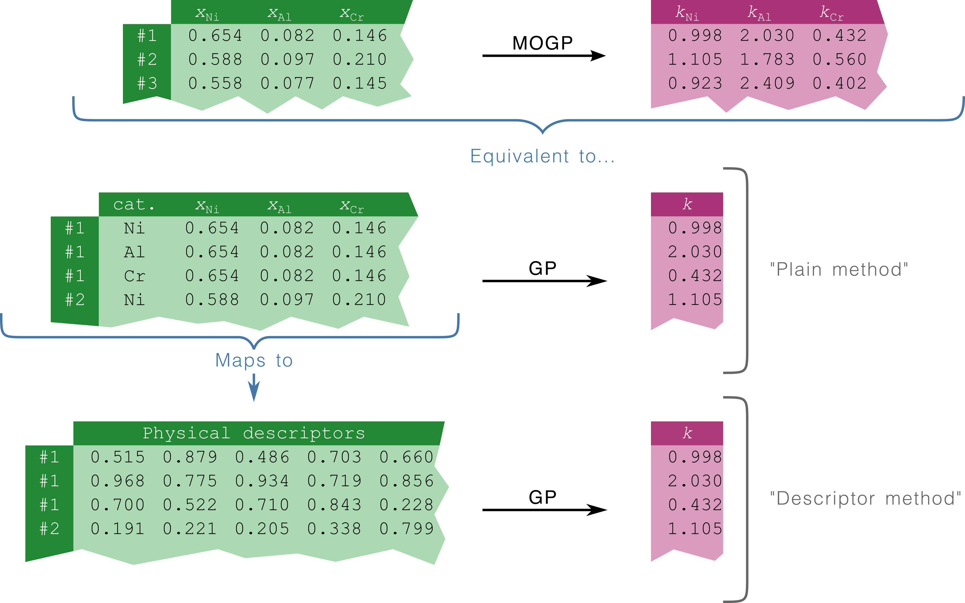
The dataset used in this work is an updated version of that in Ref. [9], containing 123 entries with complete microstructure data (matrix and precipitate phase composition and fractions) [37, 38, 39, 40, 41, 42, 43, 17, 44, 45, 46, 33, 47, 48, 49, 50, 51, 52, 53, 36, 54, 55, 56, 24, 57, 58, 59, 60, 61, 23, 62, 63, 64, 65]. The phase composition dataset is presented in the conventional form, with the nominal alloy compositions and heat treatments being the inputs to our model, and the phase fractions and respective compositions being the output. However, in this work we “reshape” the dataset into a single-target format. This is represented graphically in Fig. 1 as a two-step process. First the dataset is reshaped so that for a single-phase ML model, each partitioning coefficient is considered to be a separate output, and the input gains an additional column labelling the output element. Note that in the GPR framework, this is equivalent to a multi-output Gaussian process (MOGP) [66]. We will refer to this model as the “plain method”. Secondly, the data is transformed into a physical representation, which is a function of composition and label, but does not explicitly preserve the label as a feature. This means that predictions can be made for labels (i.e. components) not present in the training data—so long as the physical descriptors are carefully chosen. We will refer to this model as the “descriptor method”.
2.2 Physical descriptors
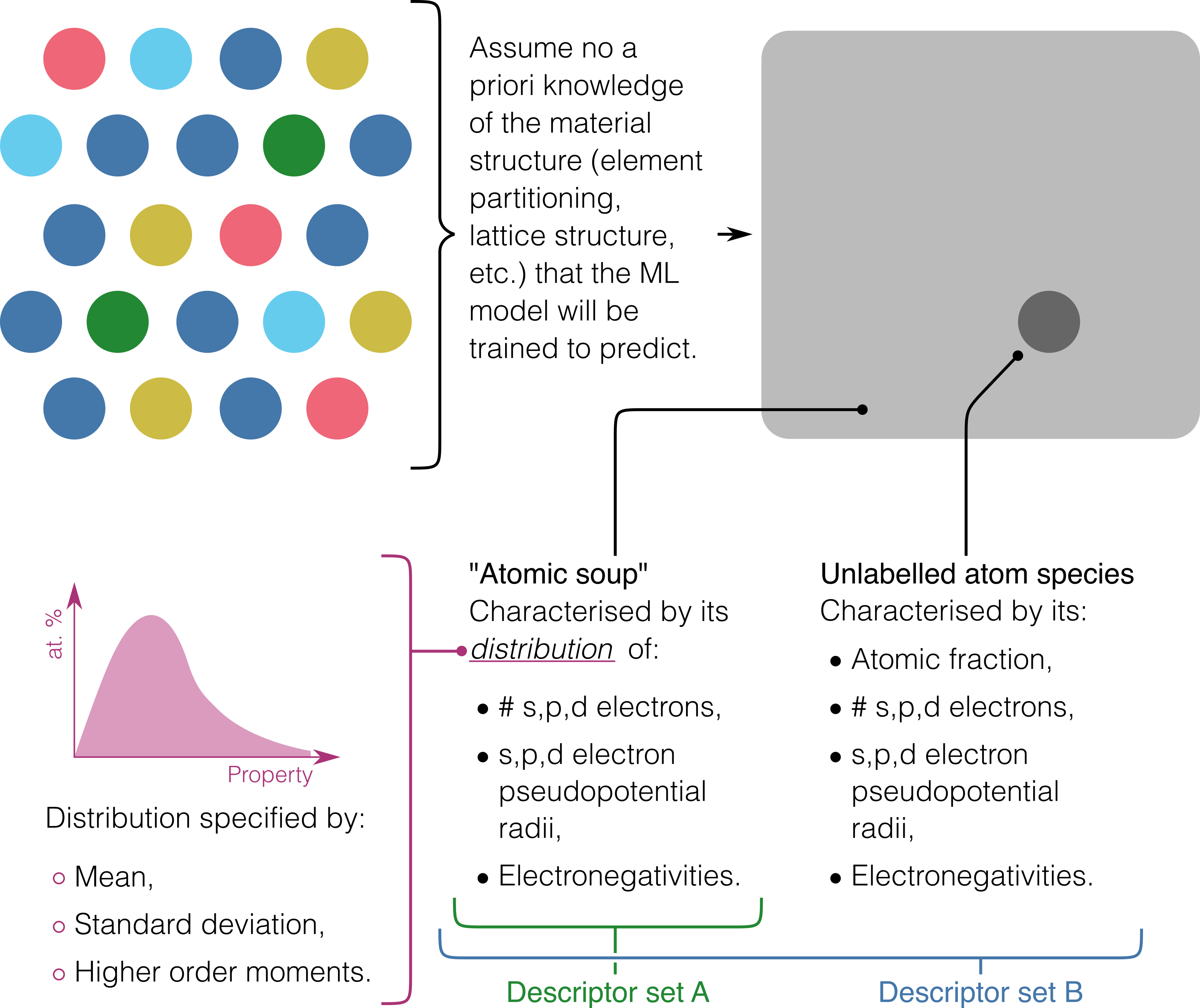
To fully understand the phase behaviour we must predict both the phase fraction, and also the partitioning of each element between the phases. The model for each property requires different inputs: for the phase fraction model, inputs were composition and heat treatment data; for the partitioning coefficient model, each entry gains a further feature corresponding to the component-label of the target, see Fig. 1 and Section 2.1. In our model, both this label and the composition are converted into element-agnostic descriptors. The most natural choice of physical descriptors would be based on the lattice structure and atomic arrangement of an alloy, but these are a priori unknown. Instead, a given alloy—for which, in our case, we only know the nominal composition—can be thought of an “atomic soup”, see Fig. 2. Inspired by ab initio electronic structure methods used in physics and chemistry, the atomic soup can be represented by the distribution of the constituent atoms’ electronic properties. Said distributions can be approximately specified by their mean, standard deviation; and higher order moments if necessary. This is how the descriptors (descriptor set A in Fig. 2) for modelling phase fraction were formulated. For the GPR model of partitioning coefficients, the atomic species labels were also transformed to physical descriptors (Fig. 1 and Section 2.1), chosen following a similar logic (descriptor set B in Fig. 2).
Our choice of descriptors bore a strong similarity to the popular descriptor-set MAGPIE [67]. Those used by Ling et al [68] and Liu et al [69] to model nickel superalloy properties are also similar. Much like these descriptor sets, we found electronic structure inspired descriptors to be especially powerful. Data used to construct our descriptors was taken from Refs. [70, 71].
Alongside its nominal composition, the precipitation heat treatments applied to an alloy will also affect its final composition and properties [9]. Up to three heat treatment stages were used as input features for each alloy; each comprising a treatment temperature () and time (), for a total of six features. The theory of Ostwald ripening gives a theoretical dependence on heat treatment time and temperature for an alloy’s phase compositions [72, 73, 74, 75]:
where is an activation energy associated with the diffusion of species . Our model’s targets are the log partitioning coefficients; heat treatment times in our database varied over several orders of magnitude (from around 15 mins to 1000 hours). Putting this altogether, we propose representing -stage heat treatments with the following descriptors:
| (1) |
This retains the same total number of descriptors as in the initial input. In Section 3.3 we show that this set of heat treatment descriptors accurately capture the evolution of the alloys’ microstructures.
2.3 Gaussian process regression
A large number of physical descriptors were proposed for use in our GPR model: much more than the number of input columns in our dataset (18 for our dataset with component and heat treatment inputs). To ensure that the GPR models were selecting the minimal set of relevant features during hyperparameter optimisation, an automatic relevance determination (ARD) Matérn kernel was used [76]. In cases where the ARD kernel lengthscale for some of the features was found to be very large, , small improvements in the model’s score could be obtained by retraining the model without using said features at all. The GPyTorch library was used for GPR [77]. Both the L-BFGS and ADAM algorithms were tested for hyperparameter optimisation, with L-BFGS being found to give both better results for a small trade-off in training time.
2.4 Probabilistic correction to phase compositions
There are three physical constraints that alloy phase compositions—i.e. the output predictions of the GPR models for phase chemistry—must obey [5, 9]:
| (2) | ||||
| (3) | ||||
| (4) |
where there are phases labelled and components labelled . Eqs. (2) & (3) are hard constraints that the total concentration and total phase fractions must each sum to unity. Eq. (4) can be interpreted as a soft constraint representing an assumption of minimal material loss in the forging process. Gaussian process regression does not present an obvious way to impose such constraints—in Ref. [9] they were imposed on the final model outputs. In particular, a Bayesian approach was taken to apply constraint Eq. (4) via a correction to the predicted phase fraction. In this work, the same approach is extended to apply a simultaneous correction to the phase fractions and the phase compositions . The output of the GPR models for phase fraction and phase composition are taken to be independent Gaussian processes, which for each alloy gives a prior:
| (5) |
and a likelihood relating to the soft constraint, where is a tolerance for ‘allowed’ component loss, and is an estimated uncertainty on the sum on the LHS of Eq. 4
| (6) |
Combining these to give a posterior, expanding the exponent of the likelihood to quadratic order in , and finally completing the square gives a new Gaussian probability distribution. This is equivalent to maximising the log-posterior probability with respect to the corrections to and . This maximisation can be carried out subject to hard constraints for Eqs. (2) & (3). Doing so produces a correction to each of and , as well as a new, valid covariance for a given prediction, which in turn yields the associated uncertainties.
2.5 Creep strength modelling
We compiled a dataset of creep strength properties for single crystal Ni superalloys. Entries were drawn from academic literature and commercial databases [39, 78, 79, 42, 17, 80, 81, 82, 83, 49, 84, 85, 86, 87, 56, 88, 89, 90, 91, 92]. A substantial contribution to the dataset was from the open source creep rupture life dataset compiled by Liu et al [69] (266 entries). Database entries included multiple properties characterising creep strength, including elongation at rupture (82 entries), time to 1% creep (79), and minimum secondary creep rate (55). There were significantly more entries available for creep rupture life (388), reflecting the importance of this particular property as the primary metric of creep strength [93, 18]. For this reason we solely focused on modelling creep rupture life. Each entry had two corresponding experimental conditions, a temperature and applied stress. Other authors have found that direct ML models of the creep rupture life are more effective than modelling the Larson-Miller parameter [13]. We adopted the same approach, which meant both experimental conditions were included as input features.
Three approaches were taken to create a GPR model for creep strength:
-
1.
Plain composition descriptors (directly analogous to the plain method described above).
-
2.
Physical descriptor set derived from the input composition only (analogous to the descriptors used for modelling phase fraction).
-
3.
Physical and metallurgical descriptors derived both from the input composition and from the fitted GPR microstructure model.
Atomistic microstructural properties, in combination with precipitate morphology, are known to determine the physical mechanisms by which creep occurs [17, 18]. This motivated the use of the third model. In this model the precipitate fraction predicted by the microstructure model was used directly as a descriptor. Other derived descriptors were used: the lattice misfit between the two phases was calculated using the Vegard coefficients [94, 95, 96]. The matrix phase stacking fault energies were approximated using fcc and hcp formation energies for each element [97, 90, 36, 18]. The formation energies were calculated via density functional theory using the PBSESOL functional [98]. The mean and standard deviation of melting points for elements in the precipitate phase were included as proxies for the solvus [99, 78]. The mean interdiffusivity metric and the mean metal d-level metrics used in the alloys-by-design procedure were also used as descriptors [100, 95, 101, 102, 103]. The necessary microstructure predictions were made using the GPR model described in the previous sections, trained on the full microstructure database excluding any entries overlapping with the creep rupture life dataset.
This GPR model incorporated more explicit high-level domain knowledge than any of the other models, which was only possible because the physical mechanisms that govern creep deformation have been well studied by metallurgists. However, the descriptors of this type that were used are not an exhaustive list, and for this reason physics-based descriptors that did not use explicit metallurgical domain knowledge were also used in this model (see Fig. 8).
3 Results
With the data curated, descriptors selected, and machine learning formalism in place, we are now well-positioned to test the performance of our machine learning algorithms. We first study the performance of microstructure prediction, before studying the creep strength.
| Phase frac. (at. %) | Composition (at. %) | |||||||
|---|---|---|---|---|---|---|---|---|
| Ni | Cr | Co | Al | Ti | Heavy els. | |||
| Phase 1 | Descriptor method | - | 4.8 | 4.8 | 3.4 | 1.7 | 1.2 | 0.6 |
| Plain method | - | 5.4 | 5.2 | 3.2 | 1.6 | 1.3 | 0.6 | |
| Phase 2 | Descriptor method | 4.4 | 3.8 | 2.7 | 2.7 | 2.4 | 1.5 | 0.5 |
| Plain method | 6.3 | 3.8 | 3.0 | 3.0 | 2.4 | 2.0 | 0.6 | |

To compare the performance of the proposed physical-descriptor model to the plain model that uses composition features, we performed two rounds of tests on the microstructure data: firstly on blind validation data where all elements had been present in the training data, and secondly for extrapolating to new materials that contain fresh elements not present in the training dataset.
3.1 Performance when all elements available
We first test the performance of the physical descriptor model when information about all elements is available at training. Two models were trained: one that uses physical descriptors as inputs and a second that inputs the plain composition. We carried out ten-fold cross validation on the available microstructure data (123 database entries). For each fold, the model was trained via log-likelihood maximisation over the training dataset, then predictions were made on the withheld validation set. These results were combined to give a single set of predictions for the entire dataset. The correction method from section 2.4 was applied in the same way to both models.
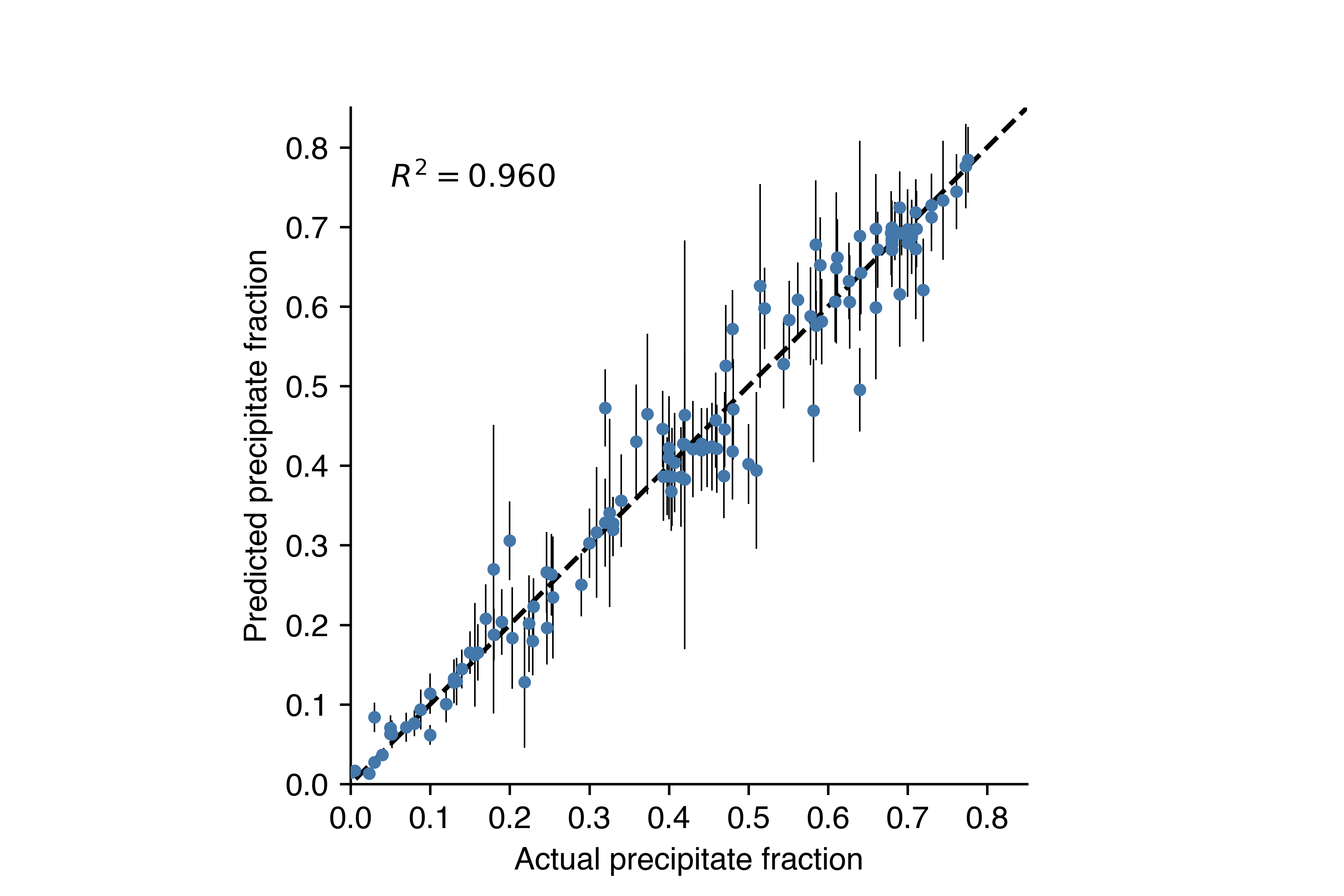
The root mean squared error (RMSE) was used to compare the two models due to its ease of interpretation for percentage-like properties. The RMSE for each element and fraction component of the microstructure is given in Table 1. The physical descriptor model was significantly better than the plain composition model for predicting phase fraction, improving the RMSE from 6.3% to 4.4%. The predicted versus actual phase fraction is plotted in Fig. 3, which confirms not only the quality of predictions, but also the accuracy of the uncertainty estimates. The phase fraction is the most crucial measure of a superalloy’s microstructure given its physical influence on yield and creep strength. The descriptor-based model shows a smaller improvement for phase composition predictions when compared with the plain method, although it does still achieve the same or better RMSE for almost every element.
We also confirmed the selected kernel hyperparameters. A Matérn kernel with smoothness parameter gave the best results for the log partitioning coefficient models and the phase fraction model. The fact that a smoother kernel gives better predictions when using physical descriptors is because the the models are ‘forced’ to find the best physical descriptors rather than relying on the kernel’s complexity to fit the data. In turn, the combination of a simpler, smoother model with a superior ‘understanding’ of chemistry allows the model to extrapolate well.
3.2 Extrapolative predictions in composition-space
To test whether descriptors improve the ability of the model to extrapolate in composition-space, we adopted the simple approach of testing our GPR model on superalloy families outside the training dataset. We focus on two categories of alloys: Re/Ru-bearing Ni-superalloys, and high-entropy superalloys (HESA).
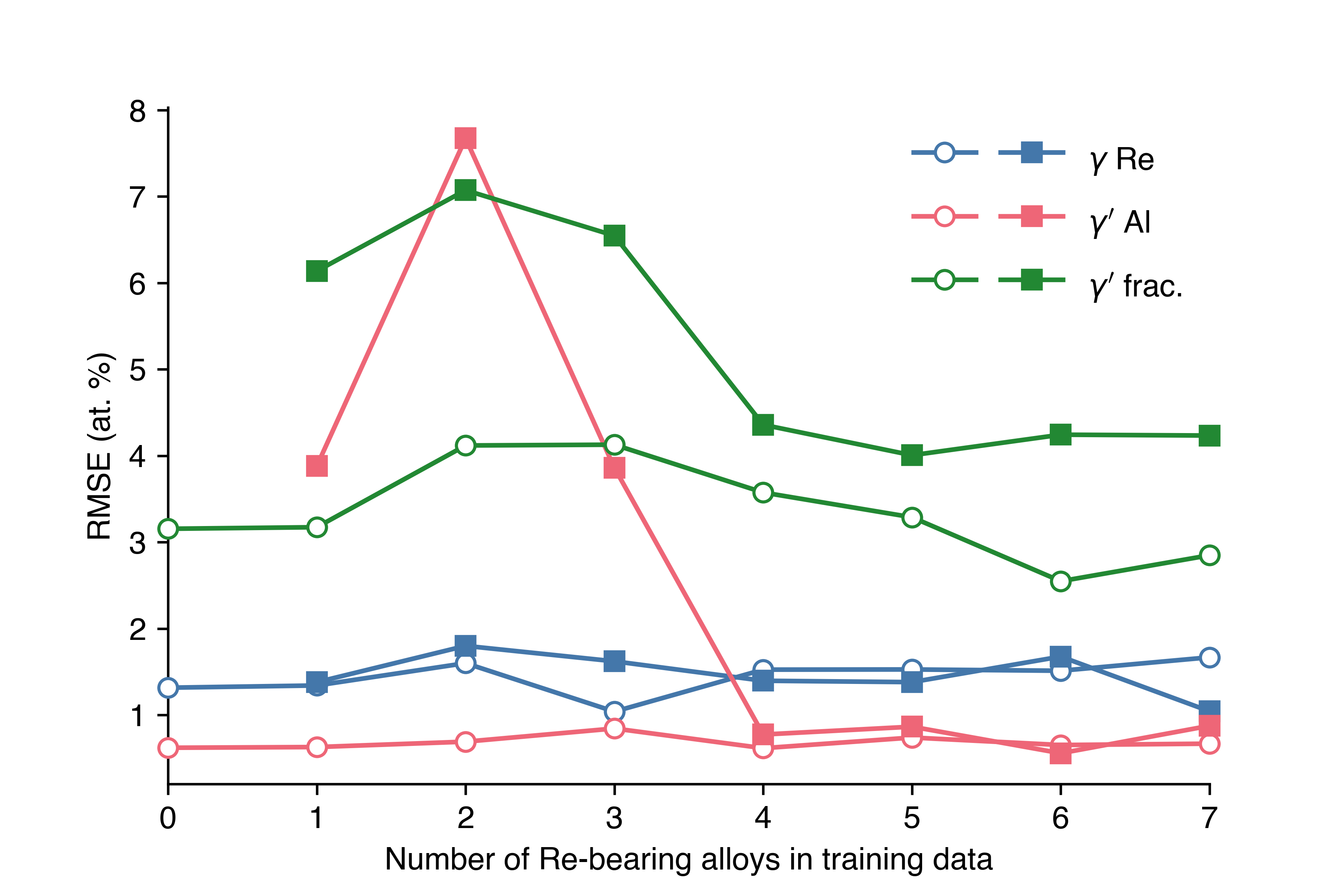
The addition of Re and Ru to commercial superalloy compositions was one of the key innovations of the most recent generations of conventionally developed single-crystal superalloys [106, 107, 108, 18]. Here we repeat the training process and start from a database comprising 88 historic superalloys that contain neither Re nor Ru. Of the data on contemporary superalloys containing Re and Ru, 6 were randomly selected to form a test set, and the remaining were added incrementally to the training set so as to expose the importance of adding fresh alloys during a research project. Fig. 4 shows the RMSE vs. number of Re-bearing alloys in the training data. The initial predictions by the physical descriptor model are extremely impressive, giving about the same RMSE on the test data as it attains with any amount of Re-bearing alloy data. When a few data-points for Re alloys are added, the plain-descriptor model overfits so gives a higher RMSE than the physical descriptor model. For the crucial prediction of the phase fraction, this improvement persists up to the maximum number of additional training data points.
High-entropy superalloys are a more recent development in alloy design, combining the design principles of high-entropy alloys and precipitation-strengthened alloys [104, 109]. HESAs typically contain Fe as one of their entropy of mixing-boosting components. For a review on HESAs see Ref. [30]. HESAs are a prime target for the physical descriptor model owing to the large number of element permutations that cannot all be represented in the training dataset. The GPR model was trained on the full conventional superalloy database, that did not contain a single HESA entry, nor any entries containing Fe. The model was then tested on the HESA data collected by Zhang et al [104] that includes Fe-bearing superalloys, with results shown in Fig. 5. The results are overall in excellent agreement, capturing the behaviour of the elements known to the model well, and notably making good predictions for Fe, which would have been impossible with the plain descriptor model. For both experimental HESAs, the RMSE for phase elements was 1.8% and for phase elements was 7.0%. Once again, predictions for the phase are better than for the phase, reflecting the stronger influence of physical factors on this phase’s formation. Such a prediction would be simply impossible to make with a plain composition descriptor model.
3.3 Heat treatments
To assess how well our heat treatment descriptors (Eq. 1) capture the evolution of microstructure during a heat treatment, we test our model against two sets of experimental data [58, 105]. In each case, the physical descriptor model was retrained on the full database excluding the respective set of test alloys.
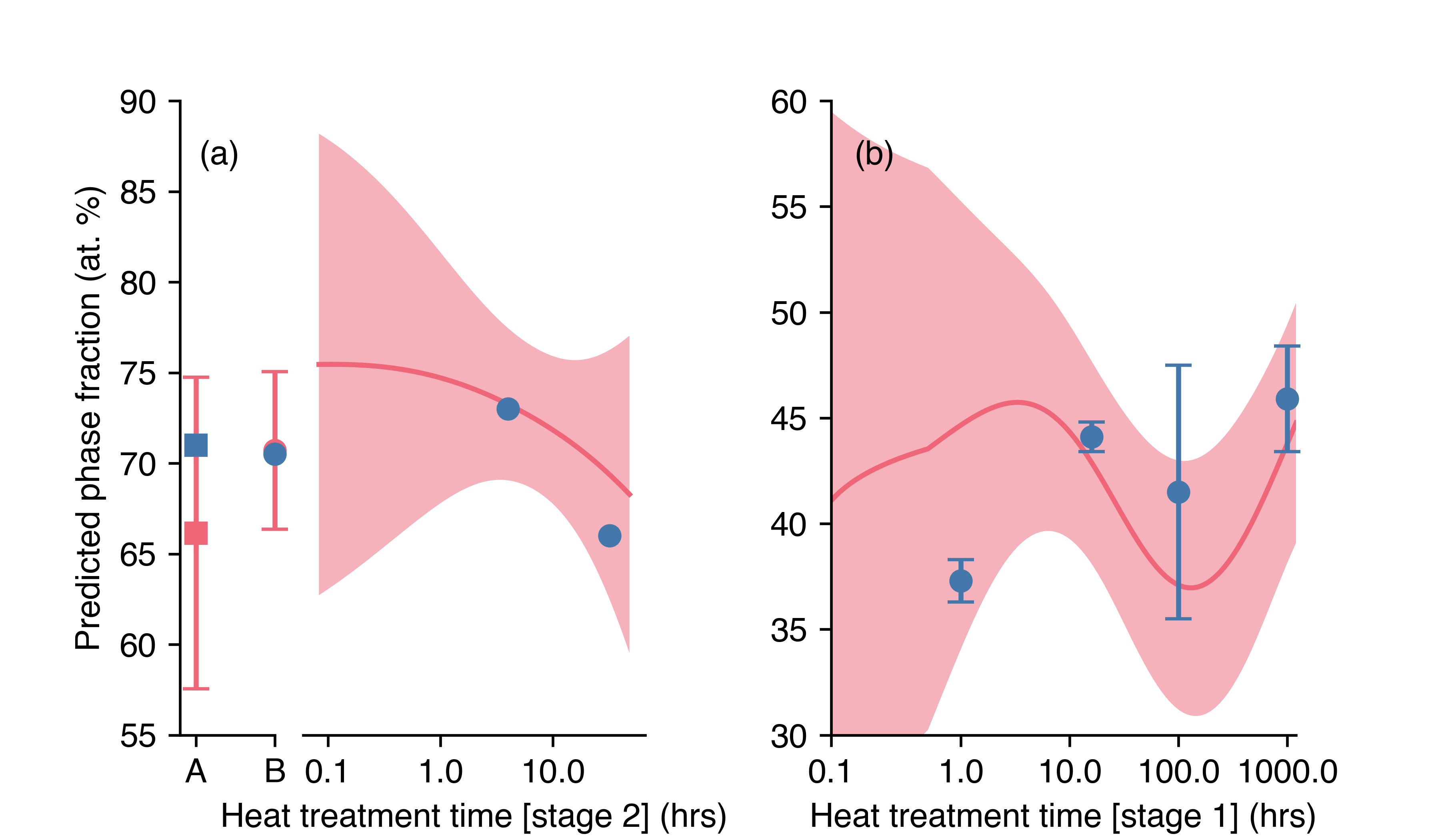
The first test case was a commercial superalloy SRR99, aged under a variety of conditions. Our model captured both the qualitative and quantitative trends in the evolution of the fraction, see Fig. 6(a). Surprisingly, it exhibited both the largest uncertainty and error for heat treatment A, the un-aged specimen. This could be reflective of a spurious correlation in the training data, since data for commercial superalloy microstructures are typically presented for fully heat treated specimens, whereas “experimental” alloy compositions are less frequently fully heat treated.
The second test case was for an experimental five-component superalloy, where each specimen was aged at for increasingly long durations, shown in Fig. 6(b). Our model captured not only the trend towards an increased phase fraction with treatment time, but also the observed decrease in precipitate fraction at intermediate ageing times. It captured this qualitative trend despite the fact that it is opposite to that observed for the alloy SRR99; which furthermore was one of the only alloys in the training data with more than two different heat treatments applied to the same composition. Our new proposed physical description of heat treatments, Eq. 1, outperformed other descriptors for both test datasets, including a plain time and temperature descriptor and other Ostwald ripening-based descriptors, as well as giving better results for the five-fold cross-validation testing described above.
3.4 Creep rupture life model
GPR models for the creep rupture life of signal crystal superalloys were trained. The accuracy of each model was assessed with ten-fold cross validation in the manner described in subsection 3.1. As the creep rupture life data spans multiple orders of magnitude, scores are given for both the actual values and log values. An ARD Matérn kernel was used in the Gaussian processes; but for the creep models, unlike those for microstructure, the optimal kernel smoothness parameter was found to be . The decreased smoothness of the kernel is likely because creep rupture life data spans multiple scales and testing regimes. For example, it is known that creep in single crystal superalloys occurs by two main mechanisms, dislocation and diffusion creep, with the former mechanism dominating at low temperatures and the latter at high temperatures.
| Descriptors | |
|---|---|
| Physics + metallurgy-based descriptor method | 0.864 |
| Physics-based descriptor method | 0.856 |
| Plain method | 0.840 |
Firstly, a plain composition descriptor GPR model was trained, which achieved . Next, a model using a similar physics-based descriptor set to that used for microstructure, i.e. using descriptors calculated solely from each alloy’s nominal overall composition, was trained. This delivered an improvement on the plain descriptor method, achieving .
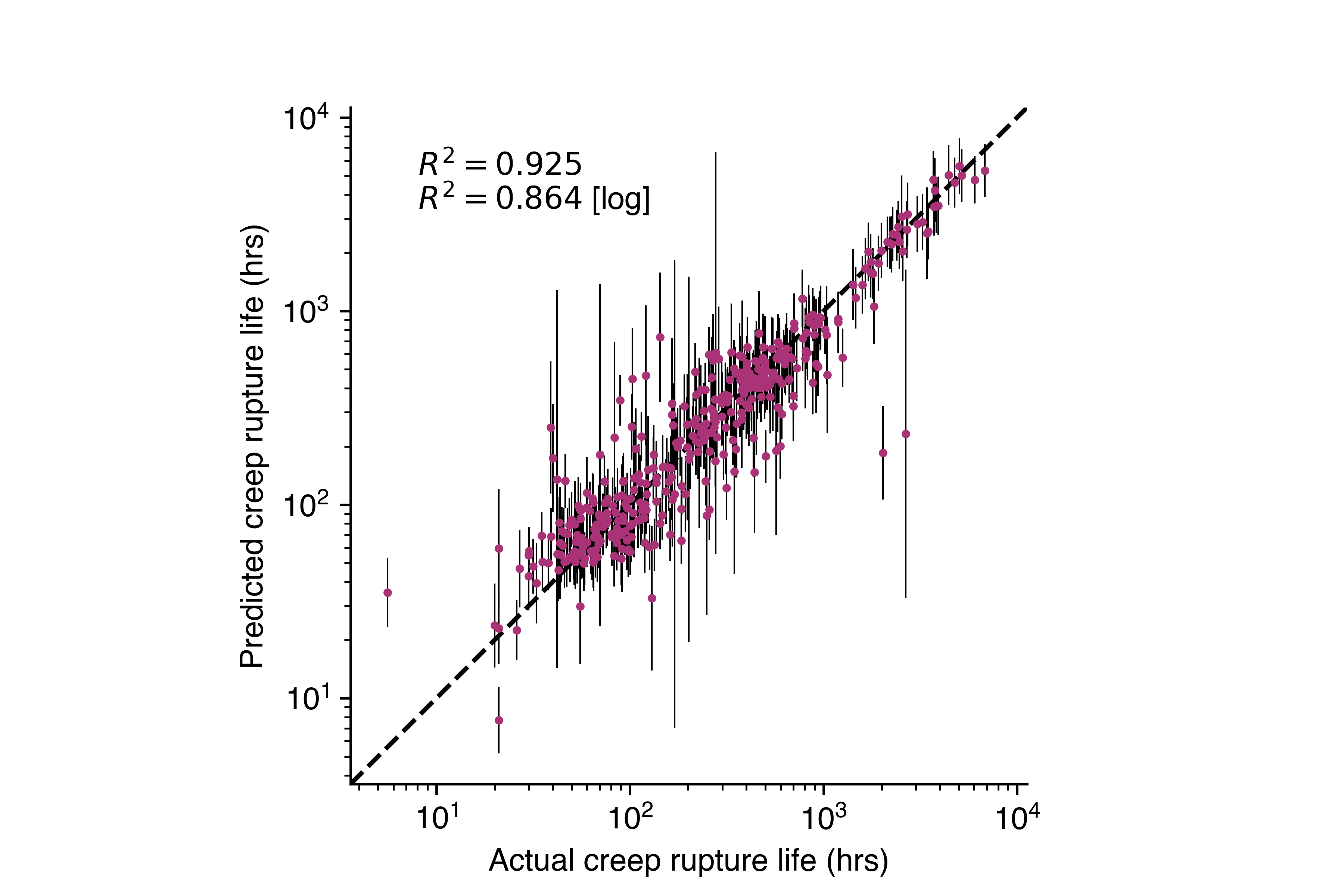
This physics-based descriptor set was then further refined to include more high-level domain knowledge, summarised in Fig. 8. Metallurgy-based descriptors developed in Section 2.5 were added, some of which were calculated using phase compositions and fractions predicted by the pre-trained microstructure model described in the preceding sections. This model achieved a further improvement of (Fig. 7).
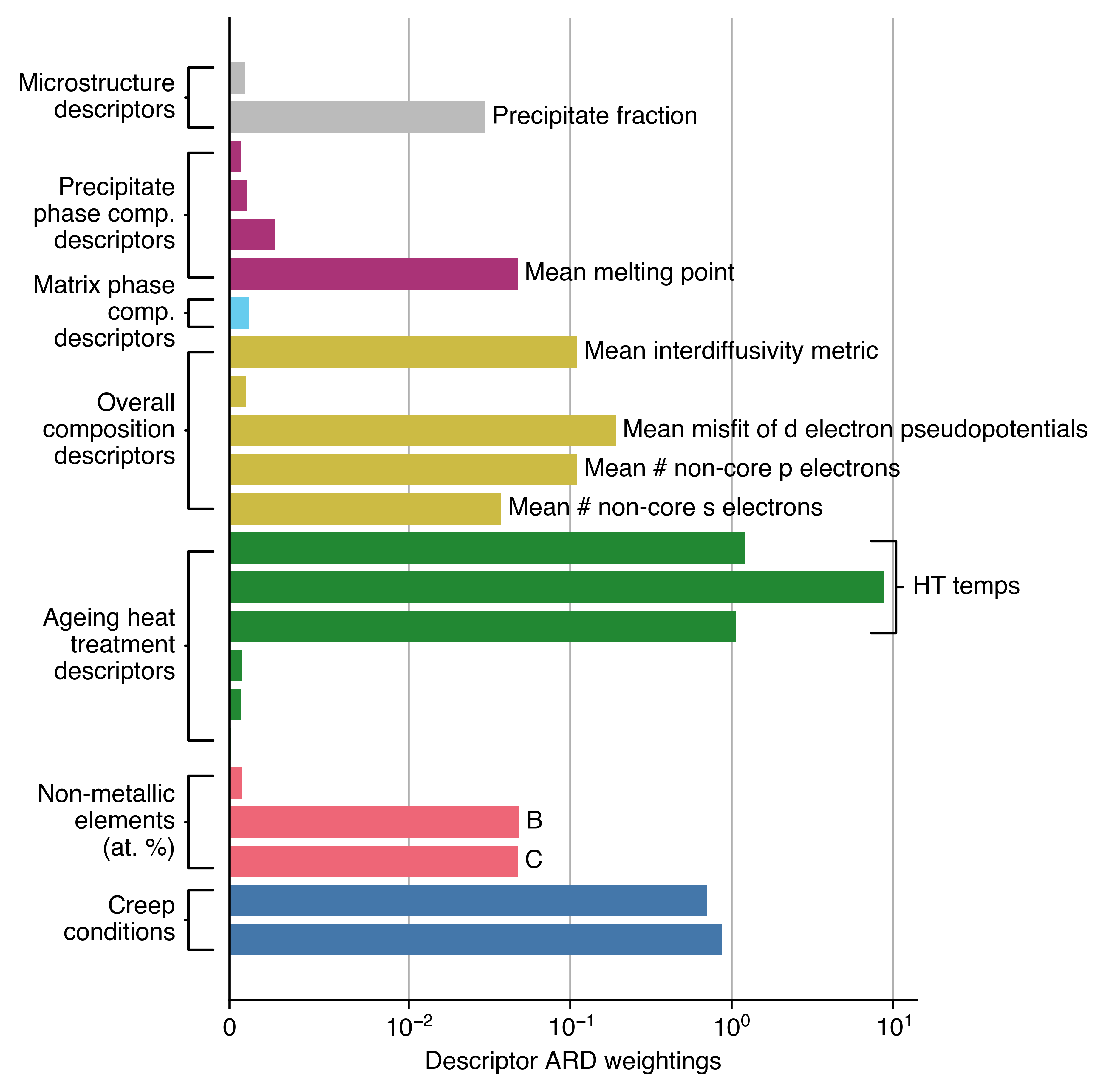
The relevance of various descriptors in this model as determined by the ARD kernel lengthscales are given in Fig. 8. Many of the expected important descriptors are found to be relevant: the precipitate fraction, the overall mean interdiffusivity, and the mean melting point of the precipitate phase are selected. However, other descriptors that were expected to be highly relevant are not selected, including the lattice misfit, mean metal d-level, and the matrix phase stacking fault energy (SFE). The mean metal d-level is a metric used to estimate susceptibility to TCP phase formation during creep: commercial single-crystal superalloys have long been designed to avoid this behaviour, which will limit the influence of this descriptor for a model fitted to a dataset of largely commercial superalloys. The matrix SFE descriptor is unlikely to be sufficiently accurate: our estimate used an average of the difference between zero-point formation energies. This neglects thermal effects and uses an approximation to the SFE in fcc alloys. The lattice misfit is likely found to be irrelevant for both of those reasons. Of the non-metallic trace elements, the B and C at. % are relevant, whereas Y is not. The same heat treatment descriptors used for the microstructure modelling were again used, but the Ostwald ripening inspired descriptors that were key to capturing microstructure evolution with ageing are not found to be relevant (although it should be noted that they indirectly enter the model via the predicted precipitate fraction descriptor). Three physics-based descriptors calculated from the nominal composition are found to be relevant. They are three descriptors that are also selected by the microstructure GPR model, so they may be relevant due to their influence on microstructure morphology, which is not explicitly modelled.
4 Conclusion
In this work we have proposed a set of physical descriptors for composition and heat treatment for use in machine learning models of superalloy microstructure. A model using physical descriptors outperforms a model using plain composition descriptors when making interpolative predictions, see Table 1. Furthermore, when making extrapolative predictions, the model significantly outperforms the plain descriptor model, notably not suffering from such a severe overfitting effect (Fig. 4). Moreover, it can also make predictions for alloys containing elements that were not even present in its training dataset (Fig. 5). Such predictions are completely impossible to make using a plain descriptor model since they are not element-agnostic. This means our model can make useful predictions for cutting-edge superalloys, such as high-entropy superalloys or superalloys containing new heavy elements.
As well as standing up on its own, our model has a number of advantages over traditional CALPHAD. Previously identified benefits include the ability to easily retrain the GPR model, incorporate non-equilibrium features such as heat treatments, and most importantly its inherent quantification of uncertainties [9]. The model presented in this work captures both qualitative and quantitative effects of ageing on microstructure, see Fig. 6(a–b). A further benefit of our model is that it is possible to easily incorporate computational data, whilst still treating it as distinct from empirical data. This can be achieved by simply adding an extra feature to the inputs: a binary descriptor encoding the method by which an entry has been obtained. The process of fitting the Gaussian process will determine how relevant the computational composition data is to predicting ‘true’ compositions.
In addition to the microstructure model, we developed a GPR model for the creep rupture life of single crystal nickel superalloys. This model builds on that developed for microstructure in two ways. Firstly, it explicitly incorporates predictions of the microstructure model as descriptors, and finds them to be relevant to making predictions, providing a direct use-case for the usefulness of our GPR approach. Secondly, it expands on the domain knowledge paradigm by making use of descriptors that encapsulate metallurgical theories and principles. By incorporating such high-level domain knowledge, the ARD lengthscales of the fitted Gaussian process can be used to infer greater physical understanding about the properties it models. With a coefficient of determination of for the log creep rupture lifes, this model is itself useful for making predictions of this key strength property of single crystal superalloys. Like the microstructure model, its predictions include uncertainties, a crucial feature for its intended usage in alloy design [110, 111, 9].
Currently our model only calculates partitioning into two pre-determined phases, a use-case we have identified as most critical to superalloy design. Other authors have constructed machine learning models to classify alloys by phase stability [14]. This points towards development of a fully-fledged, generic, and probabilistic approach to the Calculation of Phase Diagrams problem. Beyond alloys, this approach could be extended to phase separation in other systems including polymer/polymer, polymer/filler, and aqueous two-phase mixtures [112, 113, 114, 115].
CRediT authorship contribution statement
Patrick Taylor: Conceptualisation, Methodology, Software, Formal analysis, Data curation, Writing—original draft. Gareth Conduit: Conceptualisation, Methodology, Writing—review & editing, Supervision.
Declaration of competing interest
Gareth Conduit is a Director of materials machine learning company Intellegens. The authors have no other financial interests or personal relationships that could have appeared to influence the work reported in this paper.
Acknowledgements
Patrick Taylor acknowledges the financial support of EPSRC and an ICASE award from Dassault Systèmes UK. Gareth Conduit acknowledges the financial support of the Royal Society. We would also like to thank Dr. Victor Milman and Dr. Alexander Perlov at Dassault Systèmes UK for their feedback on the manuscript. There is Open Access to this paper and data available at https://www.openaccess.cam.ac.uk/.
References
-
[1]
W. Hume-Rothery, H. M. Powell,
On
the Theory of Super-Lattice Structures in Alloys, Zeitschrift für
Kristallographie - Crystalline Materials 91 (1-6) (1935) 23–47.
doi:10.1524/ZKRI.1935.91.1.23.
URL https://www.degruyter.com/document/doi/10.1524/zkri.1935.91.1.23/html - [2] W. Hume-Rothery, Atomic theory for students of metallurgy., [3d rev. reprint]. Edition, Institute of Metals. Monograph and report series, no. 3, Institute of Metals, London, 1955.
- [3] D. G. Pettifor, A chemical scale for crystal-structure maps, Solid State Communications 51 (1) (1984) 31–34. doi:10.1016/0038-1098(84)90765-8.
-
[4]
H. Glawe, A. Sanna, E. K. Gross, M. A. Marques,
The
optimal one dimensional periodic table: a modified Pettifor chemical scale
from data mining, New Journal of Physics 18 (9) (2016) 093011.
doi:10.1088/1367-2630/18/9/093011.
URL https://iopscience.iop.org/article/10.1088/1367-2630/18/9/093011https://iopscience.iop.org/article/10.1088/1367-2630/18/9/093011/meta -
[5]
U. R. Kattner,
The CALPHAD
method and its role in material and process development, Tecnologia em
Metalurgia Materiais e Mineração 13 (1) (2016) 3–15.
doi:10.4322/2176-1523.1059.
URL http://tecnologiammm.com.br/doi/10.4322/2176-1523.1059 - [6] J. O. Andersson, T. Helander, L. Höglund, P. Shi, B. Sundman, Thermo-Calc & DICTRA, computational tools for materials science, Calphad: Computer Coupling of Phase Diagrams and Thermochemistry 26 (2) (2002) 273–312. doi:10.1016/S0364-5916(02)00037-8.
- [7] S. Bajaj, A. Landa, P. Söderlind, P. E. Turchi, R. Arróyave, The U-Ti system: Strengths and weaknesses of the CALPHAD method, Journal of Nuclear Materials 419 (1-3) (2011) 177–185. doi:10.1016/j.jnucmat.2011.08.050.
-
[8]
H. Harada, H. Murakami,
Design of Ni-Base
Superalloys, in: T. Saito (Ed.), Computational Materials Design, Springer
Berlin Heidelberg, Berlin, Heidelberg, 1999, pp. 39–70.
doi:10.1007/978-3-662-03923-6{\_}2.
URL https://doi.org/10.1007/978-3-662-03923-6_2 - [9] P. L. Taylor, G. Conduit, Machine learning predictions of superalloy microstructure, Computational Materials Science 201 (2022) 110916. doi:10.1016/J.COMMATSCI.2021.110916.
- [10] B. D. Conduit, N. G. Jones, H. J. Stone, G. J. Conduit, Design of a nickel-base superalloy using a neural network, Materials and Design 131 (2017) 358–365. doi:10.1016/j.matdes.2017.06.007.
- [11] B. D. Conduit, T. Illston, S. Baker, D. V. Duggappa, S. Harding, H. J. Stone, G. J. Conduit, Probabilistic neural network identification of an alloy for direct laser deposition, Materials and Design 168 (2019) 107644. doi:10.1016/j.matdes.2019.107644.
- [12] D. Xue, D. Xue, R. Yuan, Y. Zhou, P. V. Balachandran, X. Ding, J. Sun, T. Lookman, An informatics approach to transformation temperatures of NiTi-based shape memory alloys, Acta Materialia 125 (2017) 532–541. doi:10.1016/J.ACTAMAT.2016.12.009.
-
[13]
O. Mamun, M. Wenzlick, J. Hawk, R. Devanathan,
A machine learning
aided interpretable model for rupture strength prediction in Fe-based
martensitic and austenitic alloys, Scientific Reports 2021 11:1 11 (1)
(2021) 1–9.
doi:10.1038/s41598-021-83694-z.
URL https://www.nature.com/articles/s41598-021-83694-z -
[14]
K. Lee, M. V. Ayyasamy, P. Delsa, T. Q. Hartnett, P. V. Balachandran,
Phase
classification of multi-principal element alloys via interpretable machine
learning, npj Computational Materials 2022 8:1 8 (1) (2022) 1–12.
doi:10.1038/s41524-022-00704-y.
URL https://www.nature.com/articles/s41524-022-00704-y -
[15]
R. J. Murdock, S. K. Kauwe, A. Y. T. Wang, T. D. Sparks,
Is
Domain Knowledge Necessary for Machine Learning Materials Properties?,
Integrating Materials and Manufacturing Innovation 9 (3) (2020) 221–227.
doi:10.1007/S40192-020-00179-Z/TABLES/2.
URL https://link.springer.com/article/10.1007/s40192-020-00179-z -
[16]
G. L. Hart, T. Mueller, C. Toher, S. Curtarolo,
Machine learning
for alloys, Nature Reviews Materials 2021 6:8 6 (8) (2021) 730–755.
doi:10.1038/s41578-021-00340-w.
URL https://www.nature.com/articles/s41578-021-00340-w - [17] M. Durand-Charre, The microstructure of superalloys, CRC Press, Boca Raton, Fl, USA, 1997.
- [18] R. C. Reed, The superalloys fundamentals and applications, Cambridge University Press, Cambridge, UK ; New York, 2006.
- [19] D. J. Crudden, A. Mottura, N. Warnken, B. Raeisinia, R. C. Reed, Modelling of the influence of alloy composition on flow stress in high-strength nickel-based superalloys, Acta Materialia 75 (2014) 356–370. doi:10.1016/j.actamat.2014.04.075.
- [20] E. Fleischmann, M. K. Miller, E. Affeldt, U. Glatzel, Quantitative experimental determination of the solid solution hardening potential of rhenium, tungsten and molybdenum in single-crystal nickel-based superalloys, Acta Materialia 87 (2015) 350–356. doi:10.1016/j.actamat.2014.12.011.
- [21] M. Dodaran, A. H. Ettefagh, S. M. Guo, M. M. Khonsari, W. J. Meng, N. Shamsaei, S. Shao, Effect of alloying elements on the ’ antiphase boundary energy in Ni-base superalloys, Intermetallics 117 (2 2020). doi:10.1016/j.intermet.2019.106670.
- [22] C. T. Sims, A history of superalloy metallurgy for superalloy metallurgists, in: Superalloys 1984, 1984.
- [23] S. Tin, A. C. Yeh, A. P. Ofori, R. C. Reed, S. S. Babu, M. K. Miller, Atomic partitioning of ruthenium in Ni-based superalloys, Tech. rep., Superalloys 2004: 10th International Symposium on Superalloys (2004).
- [24] R. C. Reed, A. C. Yeh, S. Tin, S. S. Babu, M. K. Miller, Identification of the partitioning characteristics of ruthenium in single crystal superalloys using atom probe tomography, Scripta Materialia 51 (4) (2004) 327–331. doi:10.1016/j.scriptamat.2004.04.019.
- [25] R. A. Hobbs, L. Zhang, C. M. Rae, S. Tin, The effect of ruthenium on the intermediate to high temperature creep response of high refractory content single crystal nickel-base superalloys, Materials Science and Engineering A 489 (1-2) (2008) 65–76. doi:10.1016/j.msea.2007.12.045.
- [26] N. Tsuno, K. Kakehi, C. M. Rae, R. Hashizume, Effect of ruthenium on creep strength of Ni-Base single-crystal superalloys at 750 ∘C and 750 MPa, Metallurgical and Materials Transactions A: Physical Metallurgy and Materials Science 40 (2) (2009) 269–272. doi:10.1007/s11661-008-9744-6.
- [27] X. G. Wang, J. L. Liu, T. Jin, X. F. Sun, The effects of ruthenium additions on tensile deformation mechanisms of single crystal superalloys at different temperatures, Materials and Design 63 (2014) 286–293. doi:10.1016/j.matdes.2014.06.009.
-
[28]
T. Tsao, Y. Chang, K. Chang, J. Yeh, M. Chiou, S. Jian, C. Kuo, W. Wang,
H. Murakami, Developing
New Type of High Temperature Alloys–High Entropy Superalloys,
International Journal of Metallurgical & Materials Engineering 1 (1) (6
2015).
doi:10.15344/2455-2372/2015/107.
URL http://dx.doi.org/10.15344/2455-2372/2015/107 - [29] J. Chen, X. Zhou, W. Wang, B. Liu, Y. Lv, W. Yang, D. Xu, Y. Liu, A review on fundamental of high entropy alloys with promising high–temperature properties (9 2018). doi:10.1016/j.jallcom.2018.05.067.
-
[30]
M. Joele, W. R. Matizamhuka, A Review on the High
Temperature Strengthening Mechanisms of High Entropy Superalloys (HESA),
Materials 14 (19) (10 2021).
doi:10.3390/MA14195835.
URL /pmc/articles/PMC8510092//pmc/articles/PMC8510092/?report=abstracthttps://www.ncbi.nlm.nih.gov/pmc/articles/PMC8510092/ - [31] M. Detrois, P. D. Jablonski, S. Antonov, S. Li, Y. Ren, S. Tin, J. A. Hawk, Design and thermomechanical properties of a ’ precipitate-strengthened Ni-based superalloy with high entropy matrix, Journal of Alloys and Compounds 792 (2019) 550–560. doi:10.1016/j.jallcom.2019.04.054.
- [32] A. M. Manzoni, U. Glatzel, New multiphase compositionally complex alloys driven by the high entropy alloy approach (1 2019). doi:10.1016/j.matchar.2018.06.036.
- [33] H. Harada, K. Ohno, T. Yamagata, T. Yokokawa, M. Yamazaki, Phase calculation and its use in alloy design program for nickel-base superalloys, Tech. rep., Superalloys 1988 (1988).
- [34] A. P. Ofori, C. J. Humphreys, S. Tin, C. N. Jones, A TEM study of the effect of platinum group metals in advanced single crystal nickel-base superalloys, Tech. rep., Superalloys 2004: 10th International Symposium on Superalloys (2004).
- [35] G. E. Fuchs, B. A. Boutwell, Modeling of the partitioning and phase transformation temperatures of an as-cast third generation single crystal Ni-base superalloy, Materials Science and Engineering A 333 (1-2) (2002) 72–79. doi:10.1016/S0921-5093(01)01825-1.
- [36] S. Ma, L. Carroll, T. M. Pollock, Development of phase stacking faults during high temperature creep of Ru-containing single crystal superalloys, Acta Materialia 55 (17) (2007) 5802–5812. doi:10.1016/j.actamat.2007.06.042.
- [37] P. A. Bagot, O. B. Silk, J. O. Douglas, S. Pedrazzini, D. J. Crudden, T. L. Martin, M. C. Hardy, M. P. Moody, R. C. Reed, An Atom Probe Tomography study of site preference and partitioning in a nickel-based superalloy, Acta Materialia 125 (2017) 156–165. doi:10.1016/J.ACTAMAT.2016.11.053.
- [38] A. Basak, S. Das, Microstructure of nickel-base superalloy MAR-M247 additively manufactured through scanning laser epitaxy (SLE), Journal of Alloys and Compounds 705 (2017) 806–816. doi:10.1016/j.jallcom.2017.02.013.
- [39] D. Blavette, P. Caron, T. Khan, An atom probe investigation of the role of rhenium additions in improving creep resistance of Ni-base superalloys, Scripta Metallurgica 20 (10) (1986) 1395–1400. doi:10.1016/0036-9748(86)90103-1.
- [40] D. Blavette, P. Duval, L. Letellier, M. Guttmann, Atomic-scale APFIM and TEM investigation of grain boundary microchemistry in astroloy nickel base superalloys, Acta Materialia 44 (12) (1996) 4995–5005. doi:10.1016/S1359-6454(96)00087-0.
-
[41]
J. P. Collier,
Effects of
replacing the refractory elements W, Nb and Ta with Mo in nickel-bases
superalloys on microstructural, microchemistry, and mechanical properties.,
Metallurgical transactions. A, Physical metallurgy and materials science 17
A (4) (1986) 651–661.
doi:10.1007/BF02643984.
URL https://link.springer.com/article/10.1007/BF02643984 - [42] F. Diologent, P. Caron, On the creep behavior at 1033 K of new generation single-crystal superalloys, Materials Science and Engineering A 385 (1-2) (2004) 245–257. doi:10.1016/j.msea.2004.07.016.
-
[43]
R. L. Dreshfield,
Estimation of gamma
phase composition in nickel-base superalloys /based on geometric analysis of
a four-component phase diagram, Tech. rep., NASA, Lewis Research Center,
Cleveland, OH, USA (1970).
URL https://ntrs.nasa.gov/search.jsp?R=19700016436 - [44] S. Duval, S. Chambreland, P. Caron, D. Blavette, Phase composition and chemical order in the single crystal nickel base superalloy MC2, Acta Metallurgica Et Materialia (1994). doi:10.1016/0956-7151(94)90061-2.
- [45] R. Glas, M. Jouiad, P. Caron, N. Clement, H. O. Kirchner, Order and mechanical properties of the matrix of superalloys, Acta Materialia (1996). doi:10.1016/S1359-6454(96)00096-1.
-
[46]
A. J. Goodfellow, E. I. Galindo-Nava, K. A. Christofidou, N. G. Jones,
T. Martin, P. A. Bagot, C. D. Boyer, M. C. Hardy, H. J. Stone,
Gamma
Prime Precipitate Evolution During Aging of a Model Nickel-Based
Superalloy, Metallurgical and Materials Transactions A: Physical Metallurgy
and Materials Science 49 (3) (2018) 718–728.
doi:10.1007/S11661-017-4336-Y/FIGURES/8.
URL https://link.springer.com/article/10.1007/s11661-017-4336-y - [47] V. Jalilvand, H. Omidvar, M. R. Rahimipour, H. R. Shakeri, Influence of bonding variables on transient liquid phase bonding behavior of nickel based superalloy IN-738LC, Materials and Design 52 (2013) 36–46. doi:10.1016/j.matdes.2013.05.042.
- [48] G. M. Janowski, R. W. Heckel, B. J. Pletka, The Effects of Tantalum on the Microstructure of Two Polycrystalline Nickel-Base Superalloys B-1900 + Hf and MAR-M247, Metallurgical Transactions A 17A (1986) 1891–1905.
- [49] T. Khan, P. Caron, C. Duret, The development and characterization of a high performance experimental single crystal superalloy, in: Superalloys 1984, Superalloys 1984, 1984, pp. 145–155.
-
[50]
O. H. Kriege, J. M. Baris,
The
chemical partitioning of elements in gamma prime separated from
precipitation-hardened, high-temperature nickel-base alloys, ASM (Amer.
Soc. Metals), Trans. Quart. (62) (1969) 195–200.
URL https://www.osti.gov/biblio/4789116-chemical-partitioning-elements-gamma-prime-separated-from-precipitation-hardened-high-temperature-nickel-base-alloys -
[51]
M. T. Lapington, D. J. Crudden, R. C. Reed, M. P. Moody, P. A. Bagot,
Characterization of Phase
Chemistry and Partitioning in a Family of High-Strength Nickel-Based
Superalloys, Metallurgical and Materials Transactions A: Physical
Metallurgy and Materials Science 49 (6) (2018) 2302–2310.
doi:10.1007/s11661-018-4558-7.
URL https://doi.org/10.1007/s11661-018-4558-7 - [52] S. C. Llewelyn, K. A. Christofidou, V. J. Araullo-Peters, N. G. Jones, M. C. Hardy, E. A. Marquis, H. J. Stone, The effect of Ni:Co ratio on the elemental phase partitioning in -’ Ni-Co-Al-Ti-Cr alloys, Acta Materialia 131 (2017) 296–304. doi:10.1016/J.ACTAMAT.2017.03.067.
- [53] W. T. Loomis, J. W. Freeman, D. L. Sponseller, The influence of molybdenum on the /’phase in experimental nickel-base superalloys, Metallurgical and Materials Transactions B 3 (4) (1972) 989–1000. doi:10.1007/bf02647677.
- [54] M. K. Miller, R. Jayaram, L. S. Lin, A. D. Cetel, APFIM characterization of single-crystal PWA 1480 nickel-base superalloy, Applied Surface Science 76-77 (C) (1994) 172–176. doi:10.1016/0169-4332(94)90339-5.
- [55] J. U. Park, S. Y. Jun, B. H. Lee, J. H. Jang, B. S. Lee, H. J. Lee, J. H. Lee, H. U. Hong, Alloy design of Ni-based superalloy with high ’ volume fraction suitable for additive manufacturing and its deformation behavior, Additive Manufacturing 52 (2022) 102680. doi:10.1016/J.ADDMA.2022.102680.
-
[56]
A. B. Parsa, P. Wollgramm, H. Buck, C. Somsen, A. Kostka, I. Povstugar, P.-P.
Choi, D. Raabe, A. Dlouhy, J. Müller, E. Spiecker, K. Demtroder,
J. Schreuer, K. Neuking, G. Eggeler,
Advanced Scale Bridging
Microstructure Analysis of Single Crystal Ni-Base Superalloys, Advanced
Engineering Materials 17 (2) (2015) 216–230.
doi:10.1002/adem.201400136.
URL http://doi.wiley.com/10.1002/adem.201400136 - [57] A. Royer, P. Bastie, M. Veron, In situ determination of ’ phase volume fraction and of relations between lattice parameters and precipitate morphology in ni-based single crystal superalloy, Acta Materialia 46 (15) (1998) 5357–5368. doi:10.1016/S1359-6454(98)00206-7.
- [58] R. Schmidt, M. Feller-Kniepmeier, Effect of heat treatments on phase chemistry of the Nickel-Base superalloy SRR 99, Metallurgical Transactions A 23 (3) (1992) 745–757. doi:10.1007/BF02675552.
- [59] M. Segersäll, P. Kontis, S. Pedrazzini, P. A. Bagot, M. P. Moody, J. J. Moverare, R. C. Reed, Thermal-mechanical fatigue behaviour of a new single crystal superalloy: Effects of Si and Re alloying, Acta Materialia 95 (2015) 456–467. doi:10.1016/j.actamat.2015.03.060.
- [60] C. K. Sudbrack, K. E. Yoon, R. D. Noebe, D. N. Seidman, Temporal evolution of the nanostructure and phase compositions in a model Ni–Al–Cr alloy, Acta Materialia 54 (12) (2006) 3199–3210. doi:10.1016/J.ACTAMAT.2006.03.015.
-
[61]
S. Sulzer, M. Hasselqvist, H. Murakami, P. Bagot, M. Moody, R. Reed,
The Effects of Chemistry
Variations in New Nickel-Based Superalloys for Industrial Gas Turbine
Applications, Metallurgical and Materials Transactions A: Physical
Metallurgy and Materials Science 51 (9) (2020) 4902–4921.
doi:10.1007/s11661-020-05845-7.
URL https://doi.org/10.1007/s11661-020-05845-7 - [62] N. Wanderka, U. Glatzel, Chemical composition measurements of a nickel-base superalloy by atom probe field ion microscopy, Materials Science and Engineering: A 203 (1-2) (1995) 69–74. doi:10.1016/0921-5093(95)09825-9.
- [63] S. T. Wlodek, M. Kelly, D. A. Alden, The Structure of Rene 88 DT, Tech. rep., Superalloys 1996 (1996).
- [64] K. E. Yoon, R. D. Noebe, D. N. Seidman, Effects of rhenium addition on the temporal evolution of the nanostructure and chemistry of a model Ni-Cr-Al superalloy. I: Experimental observations, Acta Materialia 55 (4) (2007) 1145–1157. doi:10.1016/j.actamat.2006.08.027.
- [65] Y. Zhang, N. Wanderka, G. Schumacher, R. Schneider, W. Neumann, Phase chemistry of the superalloy SC16 after creep deformation, Acta Materialia 48 (11) (2000) 2787–2793. doi:10.1016/S1359-6454(00)00099-9.
-
[66]
M. A. Álvarez, L. Rosasco, N. D. Lawrence,
Kernels for Vector-Valued
Functions: a Review, Foundations and Trends in Machine Learning 4 (3)
(2011) 195–266.
doi:10.1561/2200000036.
URL https://arxiv.org/abs/1106.6251v2 -
[67]
L. Ward, A. Agrawal, A. Choudhary, C. Wolverton,
A general-purpose
machine learning framework for predicting properties of inorganic
materials, npj Computational Materials 2016 2:1 2 (1) (2016) 1–7.
doi:10.1038/npjcompumats.2016.28.
URL https://www.nature.com/articles/npjcompumats201628 -
[68]
J. Ling, E. Antono, S. Bajaj, S. Paradiso, M. Hutchinson, B. Meredig, B. M.
Gibbons, Machine Learning for Alloy
Composition and Process Optimization, Proceedings of the ASME Turbo Expo 6
(8 2018).
doi:10.1115/GT2018-75207.
URL https://citrination.com - [69] Y. Liu, J. Wu, Z. Wang, X. G. Lu, M. Avdeev, S. Shi, C. Wang, T. Yu, Predicting creep rupture life of Ni-based single crystal superalloys using divide-and-conquer approach based machine learning, Acta Materialia 195 (2020) 454–467. doi:10.1016/j.actamat.2020.05.001.
-
[70]
J. T. Waber, D. T. Cromer,
Orbital Radii of
Atoms and Ions, The Journal of Chemical Physics 42 (12) (2004) 4116.
doi:10.1063/1.1695904.
URL https://aip.scitation.org/doi/abs/10.1063/1.1695904 - [71] Electronegativity (2021).
- [72] I. M. Lifshitz, V. V. Slyozov, The kinetics of precipitation from supersaturated solid solutions, Journal of Physics and Chemistry of Solids 19 (1-2) (1961) 35–50. doi:10.1016/0022-3697(61)90054-3.
- [73] J. E. Morral, G. R. Purdy, Particle coarsening in binary and multicomponent alloys, Scripta Metallurgica et Materialia 30 (7) (1994) 905–908. doi:10.1016/0956-716X(94)90413-8.
- [74] T. Philippe, P. W. Voorhees, Ostwald ripening in multicomponent alloys, Acta Materialia 61 (11) (2013) 4237–4244. doi:10.1016/J.ACTAMAT.2013.03.049.
- [75] M. Mostafaei, S. M. Abbasi, M. A. Mostafaei, Improvement of ’ coarsening model in high ’ volume fraction Ni-base superalloys containing different Ta/W ratio, Journal of Alloys and Compounds 885 (2021) 160938. doi:10.1016/J.JALLCOM.2021.160938.
- [76] D. K. Duvenaud, Automatic model construction with Gaussian processes, Ph.D. thesis, University of Cambridge, Cambridge (2014).
-
[77]
J. R. Gardner, G. Pleiss, D. Bindel, K. Q. Weinberger, A. G. Wilson,
GPyTorch: Blackbox Matrix-Matrix
Gaussian Process Inference with GPU Acceleration, Advances in Neural
Information Processing Systems 2018-December (2018) 7576–7586.
doi:10.48550/arxiv.1809.11165.
URL https://arxiv.org/abs/1809.11165v6 - [78] P. Caron, High ’ solvus new generation nickel-based superalloys for single crystal turbine blade applications, in: Superalloys 2000, 2000, pp. 737–746.
- [79] P. Caron, C. Ramusat, F. Diologent, Influence of the ’ fraction on the /’ topological inversion during high temperature creep of single crystal superalloys, Tech. rep., Superalloys 2008: 11th International Symposium on Superalloys (2008).
- [80] H. Harada, A. Ishida, Y. Murakami, H. K. Bhadeshia, M. Yamazaki, Atom-probe microanalysis of a nickel-base single crystal superalloy, Applied Surface Science 67 (1-4) (1993) 299–304. doi:10.1016/0169-4332(93)90329-A.
- [81] A. A. Hopgood, J. W. Martin, The Creep Behaviour of a Nickel-based Single-crystal Superalloy, Tech. rep. (1986).
- [82] O. M. Horst, D. Adler, P. Git, H. Wang, J. Streitberger, M. Holtkamp, N. Jöns, R. F. Singer, C. Körner, G. Eggeler, Exploring the fundamentals of Ni-based superalloy single crystal (SX) alloy design: Chemical composition vs. microstructure, Materials & Design 195 (2020) 108976. doi:10.1016/J.MATDES.2020.108976.
- [83] M. T. Jovanović, Z. Miškovic, B. Lukić, Microstructure and stress-rupture life of polycrystal, directionally solidified, and single crystal castings of nickel-based IN 939 superalloy, Materials Characterization 40 (4-5) (1998) 261–268. doi:10.1016/s1044-5803(98)00013-8.
- [84] T. Khan, P. Caron, Effect of processing conditions and heat treatments on mechanical properties of single-crystal superalloy CMSX-2, Materials Science and Technology (United Kingdom) 2 (5) (1986) 486–492. doi:10.1179/mst.1986.2.5.486.
- [85] Y. Koizumi, T. Kobayashi, T. Yokokawa, J. Zhang, M. Osawa, H. Harada, Y. Aoki, M. Arai, Development of next-generation Ni-base single crystal superalloys, Tech. rep., Superalloys 2004: 10th International Symposium on Superalloys (2004).
- [86] F. Liu, Z. Wang, Z. Wang, J. Zhong, X. Wu, Z. Qin, Z. Li, L. Tan, L. Zhao, L. Zhu, L. Jiang, L. Huang, L. Zhang, Y. Liu, High-throughput determination of interdiffusivity matrices in Ni-Al-Ti-Cr-Co-Mo-Ta-W multicomponent superalloys and their application in optimization of creep resistance, Materials Today Communications 24 (2020) 101018. doi:10.1016/j.mtcomm.2020.101018.
- [87] M. V. Nathal, L. J. Ebert, Elevated temperature creep-rupture behavior of the single crystal nickel-base superalloy NASAIR 100, Metallurgical Transactions A 16 (3) (1985) 427–439. doi:10.1007/BF02814341.
- [88] S. Tian, Z. Zeng, L. Fushun, C. Zhang, C. Liu, Creep behavior of a 4.5%-Re single crystal nickel-based superalloy at intermediate temperatures, Materials Science and Engineering A 543 (2012) 104–109. doi:10.1016/j.msea.2012.02.054.
-
[89]
S. Tian, B. Qian, Y. Su, H. Yu, X. Yu,
Influence of Stacking
Fault Energy on Creep Mechanism of a Single Crystal Nickel-Based Superalloy
Containing Re, Materials Science Forum 706-709 (2012) 2474–2479.
doi:10.4028/WWW.SCIENTIFIC.NET/MSF.706-709.2474.
URL https://www.scientific.net/MSF.706-709.2474 - [90] S. Tian, X. Zhu, J. Wu, H. Yu, D. Shu, B. Qian, Influence of Temperature on Stacking Fault Energy and Creep Mechanism of a Single Crystal Nickel-based Superalloy, Journal of Materials Science and Technology 32 (8) (2016) 790–798. doi:10.1016/j.jmst.2016.01.020.
- [91] J. Zhang, J. Li, T. Jin, X. Sun, Z. Hu, Effect of Mo concentration on creep properties of a single crystal nickel-base superalloy, Materials Science and Engineering A 527 (13-14) (2010) 3051–3056. doi:10.1016/j.msea.2010.01.045.
- [92] High-temperature high-strength nickel-base alloys no. 393, Tech. rep., INCO / Nickel Institute (1995).
- [93] W. Xia, X. Zhao, L. Yue, Z. Zhang, Microstructural evolution and creep mechanisms in Ni-based single crystal superalloys: A review, Journal of Alloys and Compounds 819 (2020) 152954. doi:10.1016/J.JALLCOM.2019.152954.
- [94] J. X. Zhang, J. C. Wang, H. Harada, Y. Koizumi, The effect of lattice misfit on the dislocation motion in superalloys during high-temperature low-stress creep, Acta Materialia 53 (17) (2005) 4623–4633. doi:10.1016/J.ACTAMAT.2005.06.013.
- [95] R. C. Reed, T. Tao, N. Warnken, Alloys-By-Design: Application to nickel-based single crystal superalloys, Acta Materialia 57 (19) (2009) 5898–5913. doi:10.1016/j.actamat.2009.08.018.
-
[96]
S. Neumeier, J. Ang, R. A. Hobbs, C. M. Rae, H. J. Stone,
Lattice Misfit of High
Refractory Ruthenium Containing Nickel-Base Superalloys, Advanced Materials
Research 278 (2011) 60–65.
doi:10.4028/WWW.SCIENTIFIC.NET/AMR.278.60.
URL https://www.scientific.net/AMR.278.60 -
[97]
T. Chandra, M. Ionescu, D. Mantovani,
Influence of Stacking
Fault Energy on Creep Mechanism of a Single Crystal Nickel-Based Superalloy
Containing Re, Materials Science Forum 706–709 (2012) 2474–2479.
doi:10.4028/www.scientific.net/MSF.706-709.2474.
URL https://www.scientific.net/MSF.706-709.2474 -
[98]
J. P. Perdew, A. Ruzsinszky, G. I. Csonka, O. A. Vydrov, G. E. Scuseria, L. A.
Constantin, X. Zhou, K. Burke, Restoring the
density-gradient expansion for exchange in solids and surfaces (11 2007).
doi:10.1103/PhysRevLett.100.136406.
URL http://arxiv.org/abs/0711.0156http://dx.doi.org/10.1103/PhysRevLett.100.136406 - [99] T. Grosdidier, A. Hazotte, A. Simon, Precipitation and dissolution processes in /’ single crystal nickel-based superalloys, Materials Science and Engineering A 256 (1-2) (1998) 183–196. doi:10.1016/s0921-5093(98)00795-3.
- [100] N. Yukawa, M. Morinaga, Y. Murata, H. Ezaki, S. Inoue’, High performance single crystal superalloys developed by the d-electrons concept, in: Superalloys 1988, 1988.
- [101] R. C. Reed, A. Mottura, D. J. Crudden, Alloys-By-Design: Towards Optimization of Compositions of Nickel-based Superalloys, in: Superalloys 2016, 2016, pp. 15–23.
- [102] Y. T. Tang, C. Panwisawas, J. N. Ghoussoub, Y. Gong, J. W. Clark, A. A. Németh, D. G. McCartney, R. C. Reed, Alloys-by-design: Application to new superalloys for additive manufacturing, Acta Materialia 202 (2021) 417–436. doi:10.1016/j.actamat.2020.09.023.
- [103] C. E. Campbell, W. J. Boettinger, U. R. Kattner, Development of a diffusion mobility database for Ni-base superalloys, Acta Materialia 50 (4) (2002) 775–792. doi:10.1016/S1359-6454(01)00383-4.
- [104] L. Zhang, Y. Zhou, X. Jin, X. Du, B. Li, Precipitation-hardened high entropy alloys with excellent tensile properties, Materials Science and Engineering: A 732 (2018) 186–191. doi:10.1016/J.MSEA.2018.06.102.
- [105] A. J. Goodfellow, E. I. Galindo-Nava, K. A. Christofidou, N. G. Jones, C. D. Boyer, T. L. Martin, P. A. Bagot, M. C. Hardy, H. J. Stone, The effect of phase chemistry on the extent of strengthening mechanisms in model Ni-Cr-Al-Ti-Mo based superalloys, Acta Materialia 153 (2018) 290–302. doi:10.1016/J.ACTAMAT.2018.04.064.
- [106] A. Sato, H. Harada, T. Yokokawa, T. Murakumo, Y. Koizumi, T. Kobayashi, H. Imai, The effects of ruthenium on the phase stability of fourth generation Ni-base single crystal superalloys, Scripta Materialia 54 (9) (2006) 1679–1684. doi:10.1016/J.SCRIPTAMAT.2006.01.003.
- [107] D. Argence, C. Vemault, Y. Desvallces, D. Foumier, MC-NG: A 4th generation single-crystal superalloy for future aeronautical turbine blades and vanes, in: Superalloys 2000, 2000.
-
[108]
S. Walston, A. Cetel, R. MacKay, D. Duhl, R. Dreshfield,
Joint Development of a Fourth Generation
Single Crystal Superalloy, Tech. rep., NASA (12 2004).
URL http://www.sti.nasa.gov - [109] F. Zheng, G. Zhang, X. Chen, X. Yang, Z. Yang, Y. Li, J. Li, A new strategy of tailoring strength and ductility of CoCrFeNi based high-entropy alloy, Materials Science and Engineering: A 774 (2020) 138940. doi:10.1016/J.MSEA.2020.138940.
- [110] E. J. Martin, V. R. Polyakov, L. Tian, R. C. Perez, Profile-QSAR 2.0: Kinase Virtual Screening Accuracy Comparable to Four-Concentration IC50s for Realistically Novel Compounds, Journal of Chemical Information and Modeling 57 (8) (2017) 2077–2088. doi:10.1021/acs.jcim.7b00166.
-
[111]
B. W. Irwin, J. R. Levell, T. M. Whitehead, M. D. Segall, G. J. Conduit,
Practical
Applications of Deep Learning to Impute Heterogeneous Drug Discovery Data,
Journal of Chemical Information and Modeling 60 (6) (2020) 2848–2857.
doi:10.1021/acs.jcim.0c00443.
URL https://pubs.acs.org/doi/abs/10.1021/acs.jcim.0c00443 - [112] J. Zhu, X. Lu, R. Balieu, N. Kringos, Modelling and numerical simulation of phase separation in polymer modified bitumen by phase-field method, Materials & Design 107 (2016) 322–332. doi:10.1016/J.MATDES.2016.06.041.
- [113] Y. C. Li, C. P. Wang, X. J. Liu, Thermodynamic assessments of binary phase diagrams in organic and polymeric systems, Calphad 33 (2) (2009) 415–419. doi:10.1016/J.CALPHAD.2008.12.007.
- [114] Y. Li, Thermodynamic and kinetic study of spinodal phase separation in heptane–phenol system, Calphad 50 (2015) 113–117. doi:10.1016/J.CALPHAD.2015.05.004.
- [115] A. Salabat, S. Tiani Moghadam, M. Rahmati Far, Liquid–liquid equilibria of aqueous two-phase systems composed of TritonX-100 and sodium citrate or magnesium sulfate salts, Calphad 34 (1) (2010) 81–83. doi:10.1016/J.CALPHAD.2009.12.004.