Speeding Up Multi-Objective Hyperparameter Optimization by
Task Similarity-Based Meta-Learning for the Tree-Structured Parzen Estimator

Abstract

Hyperparameter optimization (HPO) is a vital step in improving performance in deep learning (DL). Practitioners are often faced with the trade-off between multiple criteria, such as accuracy and latency. Given the high computational needs of DL and the growing demand for efficient HPO, the acceleration of multi-objective (MO) optimization becomes ever more important. Despite the significant body of work on meta-learning for HPO, existing methods are inapplicable to MO tree-structured Parzen estimator (MO-TPE), a simple yet powerful MO-HPO algorithm. In this paper, we extend TPE’s acquisition function to the meta-learning setting using a task similarity defined by the overlap of top domains between tasks. We also theoretically analyze and address the limitations of our task similarity. In the experiments, we demonstrate that our method speeds up MO-TPE on tabular HPO benchmarks and attains state-of-the-art performance. Our method was also validated externally by winning the AutoML 2022 competition on “Multiobjective Hyperparameter Optimization for Transformers”.

1 Introduction

Hyperparameter optimization (HPO) is a critical step in achieving strong performance in deep learning Chen et al. (2018); Henderson et al. (2018). Additionally, practitioners are often faced with the trade-off between important metrics, such as accuracy, latency of inference, memory usage, and algorithmic fairness Schmucker et al. (2020); Candelieri et al. (2022). However, exploring the Pareto front of multiple objectives is more complex than single-objective optimization, making it particularly important to accelerate multi-objective (MO) optimization.

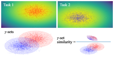
Figure 1: The conceptual visualization of $\gamma$-set similarity measure. Top row: the $\gamma$-sets of each task. The dots show the top-$\gamma$-quantile observations in both tasks. Bottom row: the $\gamma$-set similarity is measured via intersection over union of the top-$\gamma$-quantile domain, which we define $\gamma$-set; see Definition 2 in Appendix B.2 for more details.

To accelerate HPO, a large body of work on meta-learning has been actively conducted, as surveyed, e.g., by Vanschoren Vanschoren (2019). In the context of HPO, meta-learning mainly focuses on the knowledge transfer of metadata in Bayesian optimization (BO) Swersky et al. (2013); Wistuba et al. (2016); Feurer et al. (2018); Perrone et al. (2018); Salinas et al. (2020); Volpp et al. (2020). These methods use meta information in Gaussian process (GP) regression to yield more informed surrogates or an improved acquisition function (AF) for the target dataset, making them applicable to existing MO-BO methods, such as ParEGO Knowles (2006) and SMS-EGO Ponweiser et al. (2008). However, recent works reported that a variant of BO called MO tree-structured Parzen estimator (MO-TPE) Ozaki et al. (2020, 2022) is more effective than the aforementioned GP-based methods in expensive MO settings. Since MO-TPE uses kernel density estimators (KDEs) instead of GPs, existing meta-learning methods are not directly applicable, and a meta-learning procedure for TPE is yet to be explored.

To address this issue, we propose a meta-learning method for TPE on non-hierarchical spaces, i.e. search space does not include any conditional parameters, using a new task kernel. Our method models the joint probability density function (PDF) of an HP configuration $\bm{x}$ and a task $t$ using a new task kernel $k_{t}(t_{i},t_{j})$. We calculate the task kernel by using the intersection-over-union-based new similarity measure, which we call $\gamma$-set similarity, as visualized in Figure 1. Note that we describe the theoretical details in Appendix A. Although this task kernel successfully works well in many cases, its performance is degraded under some circumstances, such as for high-dimensional spaces or when transferring knowledge from slightly dissimilar tasks. To alleviate this performance degradation, we analytically discuss and address the issues in this task kernel by (1) dimension reduction based on HP importance (HPI) and (2) an $\epsilon$-greedy algorithm to determine the next HP configuration.

In our experiments, we demonstrate that our method successfully speeds up MO-TPE (or at least recovers the performance of MO-TPE when meta-tasks are not similar). The effectiveness of our method was also validated externally by winning the AutoML 2022 competition on “Multiobjective Hyperparameter Optimization for Transformers”. Note that this paper serves as the public announcement of the winner solution as well.

In summary, the main contributions of this paper are to:

1. extend TPE acquisition function (AF) to the meta-learning setting using a new task kernel,

2. discuss the drawbacks of the task kernel and provide the solutions to them, and

3. validate the performance of our method on real-world tabular benchmarks next to the external competition.

To facilitate reproducibility, our source code is available at https://github.com/nabenabe0928/meta-learn-tpe.

2 Related Work

In the context of BO, MO optimization is handled either by reducing MO to a single-objective problem (scalarization) or employing an AF that measures utility of a new configuration in the objective space. ParEGO Knowles (2006) is an example of scalarization that enjoys a convergence guarantee to the Pareto front. SMS-EGO Ponweiser et al. (2008) uses a lower-confidence bound of each objective to calculate hypervolume (HV) improvement, and EHVI Emmerich et al. (2011) uses expected HV improvement. PESMO Hernández-Lobato et al. (2016) and MESMO Wang and Jegelka (2017) are the extensions for MO settings of predictive entropy search and max-value entropy search. While those methods rely on GP, MO-TPE uses KDE and was shown to outperform the aforementioned methods in expensive MO-HPO settings Ozaki et al. (2020, 2022).

The evolutionary algorithm (EA) community also studies MO actively. MOEAs use either surrogate-assisted EAs (SAEA) Chugh et al. (2016); Guo et al. (2018); Pan et al. (2018) or non-SAEA methods. Non-SAEA methods, such as NSGA-II Deb et al. (2002) and MOEA/D Zhang and Li (2007), typically require thousands of evaluations to converge Ozaki et al. (2020), and thus SAEAs are currently more dominant in the EA domain. Since SAEAs combine an EA with a cheap-to-evaluate surrogate, SAEAs are essentially similar to BO, as they can be seen as using EAs to optimize a particular AF in BO.

Meta-learning Vanschoren (2019) is a popular method to accelerate optimization and most of them can be classified into either of the following five types in the context of HPO:

1. initialization (or warm-starting) using promising configurations in meta-tasks Feurer et al. (2015); Nomura et al. (2021),

2. search space reduction Wistuba et al. (2015); Perrone et al. (2019),

3. learning an AF Volpp et al. (2020),

4. linear combination of models trained on each task Wistuba et al. (2016); Feurer et al. (2018), and

5. training of a model jointly with meta-tasks Swersky et al. (2013); Springenberg et al. (2016); Perrone et al. (2018); Salinas et al. (2020).

Warm-starting helps especially at the early stage of optimizations but does not use knowledge from the metadata afterward. Search space reduction could be applied to any method, but cannot identify the best configurations if the target task’s optimum is outside of the optima for the meta-train tasks. The learning of AFs applies an expensive reinforcement learning step and is specific to GP-based methods. The linear combination is empirically demonstrated to outperform most meta-learning BO methods Feurer et al. (2018) including the search space reduction. The joint model trains a model on both observations and metadata. Although the linear combination of models (Type 4) is simple yet empirically strong, no meta-learning scheme for TPE has been developed so far. For this reason, we introduce a meta-learning method via a joint model (Type 5) inspired by Type 4.

3 Background

3.1 Bayesian Optimization (BO)

Suppose we would like to minimize a loss metric $f(\bm{x})$, then HPO can be formalized as follows:

$$\bm{x}_{\text{opt}}\in\mathop{\mathrm{argmin}}_{\bm{x}\in\mathcal{X}}f(\bm{x})$$ (1)

where $\mathcal{X}\coloneqq\mathcal{X}_{1}\times\dots\mathcal{X}_{D}\subseteq\mathbb{R}^{D}$ is the search space and $\mathcal{X}_{d}\subseteq\mathbb{R}$ ($d=1,\dots,D$) is the domain of the $d$-th HP. In Bayesian optimization (BO) Brochu et al. (2010); Shahriari et al. (2016); Garnett (2022), we assume that $f(\bm{x})$ is expensive, and we consider the optimization in a surrogate space given observations $\mathcal{D}$. First, we build a predictive model $p(f|\bm{x},\mathcal{D})$. Then, the optimization in each iteration is replaced with the optimization of the so-called AF. A common choice for the AF is the following expected improvement Jones et al. (1998):

$$\mathrm{EI}_{f^{\star}}[\bm{x}|\mathcal{D}]=\int_{-\infty}^{f^{\star}}(f^{\star}-f)p(f|\bm{x},\mathcal{D})df.$$ (2)

Another common choice is the following probability of improvement (PI) Kushner (1964):

$$\mathbb{P}[f\leq f^{\star}|\bm{x},\mathcal{D}]=\int_{-\infty}^{f^{\star}}p(f|\bm{x},\mathcal{D})df.$$ (3)

3.2 Tree-Structured Parzen Estimator (TPE)

TPE Bergstra et al. (2011, 2013) is a variant of BO methods and it uses the expected improvement. See Watanabe Watanabe (2023b) to better understand the algorithm components. To transform Eq. (2), we define the following:

$$p(\bm{x}|f,\mathcal{D})\coloneqq\left\{\begin{array}[]{ll}p(\bm{x}|\mathcal{D}^{(l)})&(f\leq f^{\gamma})\\ p(\bm{x}|\mathcal{D}^{(g)})&(f>f^{\gamma})\end{array}\right.$$ (6)

where $\mathcal{D}^{(l)},\mathcal{D}^{(g)}$ are the observations with $f(\bm{x}_{n})\leq f^{\gamma}$ and $f(\bm{x}_{n})>f^{\gamma}$, respectively. $f^{\gamma}$ is determined such that $f^{\gamma}$ is the $\lceil\gamma|\mathcal{D}|\rceil$-th best observation in $\mathcal{D}$. Note that $p(\bm{x}|\mathcal{D}^{(l)}),p(\bm{x}|\mathcal{D}^{(g)})$ are built by KDE. Combining Eqs. (2), (6) and Bayes’ theorem, the AF of TPE is computed as Bergstra et al. (2011):

$$\mathrm{EI}_{f^{\gamma}}[\bm{x}|\mathcal{D}] \stackrel{{\scriptstyle\mathrm{rank}}}{{\simeq}}\frac{p(\bm{x}|\mathcal{D}^{(l)})}{p(\bm{x}|\mathcal{D}^{(g)})}.$$ (7)

Note that $\phi(\bm{x})\stackrel{{\scriptstyle\mathrm{rank}}}{{\simeq}}\psi(\bm{x})$ implies the order isomorphic and $\forall\bm{x},\bm{x}^{\prime}\in\mathcal{X},\phi(\bm{x})\leq\phi(\bm{x}^{\prime})\Leftrightarrow\psi(\bm{x})\leq\psi(\bm{x}^{\prime})$ holds. In each iteration, TPE samples configurations from $p(\bm{x}|\mathcal{D}^{(l)})$ and takes the configuration that satisfies the maximum density ratio among the samples. Note that although our task kernel cannot be computed for tree-structured search space, a.k.a. non-hierarchical search space, we use the name tree-structured Parzen estimator because this name is already recognized as a BO method using the density ratio of KDEs.

3.3 Multi-Objective TPE (MO-TPE)

MO-TPE Ozaki et al. (2020, 2022) is a generalization of TPE with MO settings which falls back to the original TPE in case of single-objective settings. MO-TPE also uses the density ratio $p(\bm{x}|\mathcal{D}^{(l)})/p(\bm{x}|\mathcal{D}^{(g)})$ and picks the configuration with the best AF value at each iteration. The only difference from the original TPE is the split algorithm of $\mathcal{D}$ into $\mathcal{D}^{(l)}$ and $\mathcal{D}^{(g)}$. MO-TPE uses the HV subset selection problem (HSSP) Bader and Zitzler (2011) to obtain $\mathcal{D}^{(l)}$. HSSP tie-breaks configurations with the same non-domination rank based on the HV contribution. MO-TPE is reduced to the original TPE when we apply it to a single objective problem. In this paper, we replace HSSP with a simple tie-breaking method based on the crowding distance Deb et al. (2002) as this method does not require HV calculation, which can be highly expensive.

4 Meta-Learning for TPE

In this section, we briefly explain the TPE formulation and then describe the formulation of the AF for the meta-learning setting. Note that our method can be easily extended to MO settings using a rank metric $R:\mathbb{R}^{m}\rightarrow\mathbb{R}$ of an objective vector $\bm{f}\in\mathbb{R}^{m}$, and thus we discuss our formulation for the single-objective setting for simplicity; see Appendix B.3 for the theoretical discussion of the extension to MO settings.

Throughout this paper, we denote metadata as $\bm{D}\coloneqq\{\mathcal{D}_{m}\}_{m=1}^{T}$, where $T\in\mathbb{N}$ is the number of tasks and $\mathcal{D}_{m}$ is the set of observations on the $m$-th task with size $N_{m}\coloneqq|\mathcal{D}_{m}|$. We use the notion of the $\gamma$-set, which is, roughly speaking, a set of top-$\gamma$ quantile configurations as visualized in Figure 1; for more theoretical details, see Appendix B.2. Furthermore, we define $\mathcal{X}^{\gamma}_{m}$ as the $\gamma$-set of the $m$-th task. For example, the red regions and the blue regions in Figure 1 correspond to $\mathcal{X}^{\gamma}_{1}$ and $\mathcal{X}^{\gamma}_{2}$.

4.1 Task-Conditioned Acquisition Function

TPE Bergstra et al. (2011) first splits a set of observations $\mathcal{D}=\{(\bm{x}_{n},f(\bm{x}_{n}))\}_{n=1}^{N}$ into $\mathcal{D}^{(l)}$ and $\mathcal{D}^{(g)}$ at the top-$\gamma$ quantile. Then we build KDEs $p(\bm{x}|\mathcal{D}^{(l)})$ and $p(\bm{x}|\mathcal{D}^{(g)})$, and compute the AF via $p(\bm{x}|\mathcal{D}^{(l)})/p(\bm{x}|\mathcal{D}^{(g)})$. The following proposition provides the multi-task version of the AF:

Proposition 1

Under the assumption of the conditional shift, the task-conditioned $\mathrm{AF}$ is computed as$\mathrm{:}$

$$\mathrm{EI}_{f^{\gamma}}[\bm{x}|t,\bm{D}]\stackrel{{\scriptstyle\mathrm{rank}}}{{\simeq}}\frac{p(\bm{x},t|\bm{D}^{(l)})}{p(\bm{x},t|\bm{D}^{(g)})}.$$ (8)

The conditional shift means that $p(\bm{x}|y,t_{i})=p(\bm{x}|y,t_{j})$ holds for different tasks, i.e. $t_{i}\neq t_{j}$ and it holds in our formulation due to the classification nature of the TPE model. We discuss more details in Appendix A.1. This formulation transfers the knowledge of top domains and weights the knowledge from similar tasks more. To compute the AF, we need to model the joint PDFs $p(\bm{x},t|\mathcal{D}^{(l)}),p(\bm{x},t|\mathcal{D}^{(g)})$, which we thus discuss in the next section.

4.2 Task Kernel

To compute the task kernel $k_{t}(t_{i},t_{j})$, the $\gamma$-set similarity visualized in Figure 1 (see Appendix B.2 for the formal definition) is employed. From Theorem 26 in Appendix A.2,

$$\hat{s}(\mathcal{D}^{(l)}_{i},\mathcal{D}^{(l)}_{j})\coloneqq\frac{1-d_{\mathrm{tv}}(p_{i},p_{j})}{1+d_{\mathrm{tv}}(p_{i},p_{j})}$$ (9)

almost surely converges to the $\gamma$-set similarity $s(\mathcal{X}^{\gamma}_{i},\mathcal{X}^{\gamma}_{j})$ if we can guarantee the strong consistency of $p(\bm{x}|\mathcal{D}^{(l)}_{m})$ for all $m=1,\dots,T$ where we define $p_{m}\coloneqq p(\bm{x}|\mathcal{D}^{(l)}_{m})$, $t_{m}$ as a meta-task for $m=2,\dots,T$ and $t_{1}$ as the target task,

$$d_{\mathrm{tv}}(p_{i},p_{j})\coloneqq\frac{1}{2}\int_{\bm{x}\in\mathcal{X}}|p(\bm{x}|\mathcal{D}^{(l)}_{i})-p(\bm{x}|\mathcal{D}^{(l)}_{j})|d\bm{x}$$ (10)

is the total variation distance, and $p(\bm{x}|\mathcal{D}^{(l)}_{i})$ is estimated by KDE. Note that $d_{\mathrm{tv}}(p_{i},p_{j})$ is approximated simply via Monte-Carlo sampling. In short, we need to compute:

1. KDEs of the top-$\gamma$-quantile observations in $\mathcal{D}_{m}$, and

2. $d_{\mathrm{tv}}$ between the target task and each meta-task.

Then we define the task kernel as follows:

$$k_{t}(t_{i},t_{j})=\left\{\begin{array}[]{ll}\frac{1}{T}\hat{s}(\mathcal{D}^{(l)}_{i},\mathcal{D}^{(l)}_{j})&(i\neq j)\\ 1-\frac{1}{T}\sum_{k\neq i}\hat{s}(\mathcal{D}^{(l)}_{i},\mathcal{D}^{(l)}_{k})&(i=j)\end{array}\right..$$ (13)

Note that our task kernel is not strictly a kernel function as our task kernel does not satisfy semi-positive definite although it is still symmetric. The kernel is defined so that the summation over all tasks is $1$, and then KDEs are built as follows:

$$p(\bm{x},t|\bm{D}^{\prime}) =\frac{1}{N_{\mathrm{all}}^{\prime}}\sum_{m=1}^{T}k_{t}(t,t_{m})\sum_{n=1}^{N_{m}^{\prime}}k_{x}(\bm{x},\bm{x}_{m,n})$$ (14)

$$=\frac{1}{N_{\mathrm{all}}^{\prime}}\sum_{m=1}^{T}N_{m}^{\prime}k_{t}(t,t_{m})p(\bm{x}|\mathcal{D}_{m}^{\prime}),$$

where $\bm{D}^{\prime}\coloneqq\{\mathcal{D}_{m}^{\prime}\}_{m=1}^{T}$ is a set of subsets of the observations on the $m$-th task $\mathcal{D}^{\prime}_{m}=\{(\bm{x}_{m,n},f_{m}(\bm{x}_{m,n}))\}_{n=i}^{i+N^{\prime}_{m}-1}$, and $N_{\mathrm{all}}^{\prime}=\sum_{m=1}^{T}N_{m}^{\prime}$. In principle, $\mathcal{D}^{\prime}_{m}$ could be either $\mathcal{D}^{(l)}_{m}$ or $\mathcal{D}^{(g)}_{m}$. The advantages of this formulation are to (1) not be affected by the information from another task $t_{m}$ if the task is dissimilar from the target task $t_{1}$, i.e. $\hat{s}(t_{1},t_{m})=0$, and (2) asymptotically converge to the original formulation as the sample size goes to infinity, i.e. $\lim_{N_{1}^{\prime}\rightarrow\infty}p(\bm{x},t|\bm{D}^{\prime})=p(\bm{x}|\mathcal{D}^{\prime}_{1})$.

Algorithm 1 Task kernel (after the modifications)

1:$\eta$ (controls the dimension reduction amount), $S$ (Sample size of Monte-Carlo sampling)

2:$l_{m}(\bm{x})\coloneqq p(\bm{x}|\mathcal{D}^{(l)}_{m})$ for $m=1,\dots,T$

3:for $d=1,\dots,D$ do$\triangleright$ Dimension reduction

4:     Calculate the average HPI $\bar{\mathbb{V}}_{d}$ based on Eq. (15)

5:$\triangleright$ Pick dimensions from higher $\bar{\mathbb{V}}_{d}$

6:Build $\mathcal{S}$ with the top-$\lfloor\log_{\eta}|\mathcal{D}^{(l)}_{1}|\rfloor$ dimensions

7:Re-build $p^{\mathrm{DR}}_{m}(\bm{x}|\mathcal{D}^{(l)}_{m})$ based on Eq. (17)

8:for $m=2,\dots,T$ do

9:     $\triangleright$ Use $S$ samples for Monte-Carlo sampling

10:     Calculate $d_{\mathrm{tv}}$ in Eq. (10) with $l^{\mathrm{DR}}_{1},l^{\mathrm{DR}}_{m}$

11:     Calculate $k_{t}(t_{1},t_{m})$ based on Eq. (13)

12:return $k_{t}$

Algorithm 2 Meta-learning TPE

1:$N_{\mathrm{init}}$ (the number of initial samples), $N_{s}$ (the number of candidates for each iteration), $\gamma$ (the quantile to split $\mathcal{D}_{\cdot}$), $\epsilon$ (the ratio of random sampling), $\mathcal{D}_{m}$ (metadata)

2:$\mathcal{D}_{1}\leftarrow\emptyset,\mathcal{D}_{\mathrm{init}}\leftarrow\emptyset$

3:for $m=2,\dots,T$ do $\triangleright$ Create a warm-start set

4:     Add the top $\lceil N_{\mathrm{init}}/(T-1)\rceil$ in $\mathcal{D}_{m}$ to $\mathcal{D}_{\mathrm{init}}$

5:     $\triangleright$ Build KDEs for meta-tasks

6:     Sort $\mathcal{D}_{m}$ and build KDEs $p(\bm{x}|\mathcal{D}^{(l)}_{m}),p(\bm{x}|\mathcal{D}^{(g)}_{m})$

7:for $n=1,\dots,N_{\mathrm{init}}$ do $\triangleright$ Initialization by warm-start

8:     Randomly pick $\bm{x}$ from $\mathcal{D}_{\mathrm{init}}$

9:     Pop $\bm{x}$ from $\mathcal{D}_{\mathrm{init}}$

10:     $\mathcal{D}_{1}\leftarrow\mathcal{D}_{1}\cup\{(\bm{x},f_{1}(\bm{x}))\}$

11:while Budget is left do

12:     $\mathcal{S}=\emptyset$

13:     Sort $\mathcal{D}_{1}$ and build KDEs $p(\bm{x}|\mathcal{D}^{(l)}_{1}),p(\bm{x}|\mathcal{D}^{(g)}_{1})$

14:     for $m=1,\dots,T$ do

15:         $\{\bm{x}_{j}\}_{j=1}^{N_{s}}\sim p(\bm{x}|\mathcal{D}^{(l)}_{m}),\mathcal{S}\leftarrow\mathcal{S}\cup\{\bm{x}_{j}\}_{j=1}^{N_{s}}$      

16:      Calculate the task kernel $k_{t}$ by Algorithm 1

17:     if $r\leq\epsilon$ then$\triangleright$ $r\sim\mathcal{U}(0,1)$, $\epsilon$-greedy algorithm

18:         Randomly sample $\bm{x}$ and set $\bm{x}_{\text{opt}}\leftarrow\bm{x}$

19:     else

20:         Pick $\bm{x}_{\text{opt}}\in\mathop{\mathrm{argmax}}_{\bm{x}\in\mathcal{S}}\mathrm{EI}_{f^{\gamma}}[\bm{x}|t_{1},\bm{D}]$ $\triangleright$ Eq. (8)      

21:     $\mathcal{D}_{1}\leftarrow\mathcal{D}_{1}\cup\{(\bm{x}_{\text{opt}},f_{1}(\bm{x}_{\text{opt}}))\}$

4.3 When Does Our Meta-Learning Fail?

In this section, we discuss the drawbacks of our meta-learning method and provide solutions for them.

4.3.1 Case I: $\gamma$-Set for Target Task $\mathcal{D}^{(l)}_{1}$ Does Not Approach $\mathcal{X}^{\gamma}$

From the assumption of Theorem 26, $\mathcal{D}^{(l)}_{1}$ must approach $\mathcal{X}^{\gamma}$ to approximate the $\gamma$-set similarity precisely; however, since TPE is not a uniform sampler and it is a local search method due to the fact that the AF of TPE is PI Watanabe and Hutter (2022, 2023); Song et al. (2022), it does not guarantee that $\mathcal{D}^{(l)}_{1}$ goes to $\mathcal{X}^{\gamma}$ and it may even be guided towards non-$\gamma$-set domains. In this case, our task similarity measure not only obtains a wrong approximation, but also causes poor solutions. To avoid this problem, we introduce the $\epsilon$-greedy algorithm to pick the next configuration instead of the greedy algorithm. By introducing the $\epsilon$-greedy algorithm, we obtain the following theorem, and thus we can guarantee more correct or tighter similarity approximation:

Theorem 1

If we use the $\epsilon$-greedy policy ($\epsilon\in(0,1)$) for $\mathrm{TPE}$ to choose the next candidate $\bm{x}$ for a noise-free objective function $f(\bm{x})$ defined on search space $\mathcal{X}$ with at most a countable number of configurations, and we use a $\mathrm{KDE}$ whose distribution converges to the empirical distribution as the number of samples goes to infinity, then a set of the top-$\gamma$-quantile observations $\mathcal{D}^{(l)}_{1}$ is almost surely a subset of $\mathcal{X}^{\gamma}$.

The proof is provided in Appendix B.5. Intuitively speaking, this theorem states that when we use the $\epsilon$-greedy algorithm, $\mathcal{D}^{(l)}_{1}$ will not include any configurations worse than the top-$\gamma$ quantile if we have a sufficiently large number of observations. Therefore, the task similarity is correctly or pessimistically estimated. Notice that we use the bandwidth selection used by Falkner et al. Falkner et al. (2018), which satisfies the assumption about the KDE in Theorem 1.

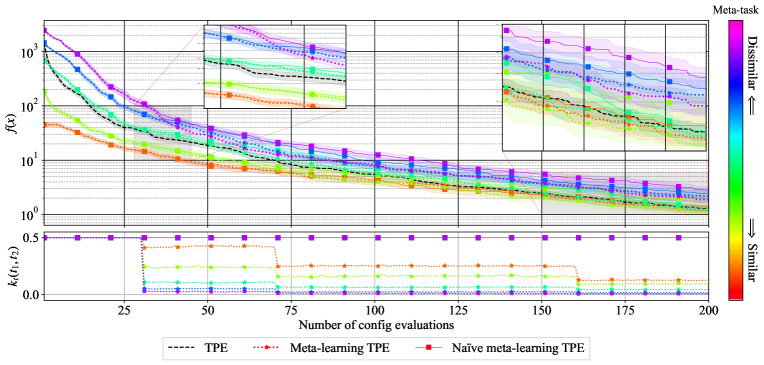
Figure 2: The comparison of the convergence of TPE and meta-learning TPE based on the task similarity. $c^{\star}=0$ is identical to the target task and tasks become dissimilar as $c^{\star}$ becomes larger. Top: each line except the black line is the performance curves of meta-learning TPE on differently similar tasks (orange is similar and purple is dissimilar). Dotted lines with $\star$ markers are for meta-learning TPE and solid lines with $\blacksquare$ markers are for naïve meta-learning TPE. Weak-color bands show the standard error of the objective function value over $50$ independent runs. Bottom: the medians of the task weight on the meta-task (higher is similar).

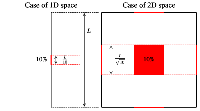
Figure 3: The conceptual visualization where the top-$10\%$ domain for each dimension becomes larger when the importance of each dimension is same and there is no interaction between dimensions. The thick black lines are the edges of each domain and the red lines are the important domains for each dimension. The red lines become longer as the dimensionality becomes higher and it implies that the marginal $\gamma$-set PDF approaches the uniform PDF as $D$ goes to $\infty$.

4.3.2 Case II: Search Space Dimension $D$ Is High

When the dimensionality $D$ is high, the approximation of the $\gamma$-set similarity is easily biased. In Figure 3, we provide a concrete example, where we consider $f(\bm{x})=\|R\bm{x}\|_{1}$. Note that $\bm{x}\in[-1/2,1/2]^{D}$ and $R\in\mathbb{R}^{D\times D}$ is the rotation matrix in this example. The $\gamma$-set of this example is $\mathcal{X}^{\gamma}=[-\gamma^{1/D}/2,\gamma^{1/D}/2]$. As $\lim_{D\rightarrow\infty}\gamma^{1/D}=1$, which can be seen from the fact that the red lines become longer in 2D case, the marginal $\gamma$-set PDF $p_{d}(x_{d}|\mathcal{D}^{(l)})\coloneqq\int_{\bm{x}_{-d}\in\mathcal{X}_{-d}}p(\bm{x}|\mathcal{D}^{(l)})d\bm{x}_{-d}$ for each dimension (roughly speaking, the red lines for each dimension in Figure 3 show the region where the marginal $\gamma$-set PDF exhibits high density) approaches the uniform PDF in this example. However, the marginal $\gamma$-set PDF for each dimension will not converge to the uniform PDF when we have only a few observations. In fact, it is empirically known that the effective dimension $D_{e}$ in HPO is typically much lower than $D$ Bergstra and Bengio (2012). This could imply that the marginal $\gamma$-set PDF for most dimensions go to the uniform PDF and only a fraction of dimensions have non-uniform PDF. In such cases, the following holds:

Proposition 2

If some dimensions are trivial on two tasks, the $\gamma$-set similarity between those tasks is identical irrespective of with or without those dimensions.

Roughly speaking, a trivial dimension is a dimension that does not contribute to $f(\bm{x})$ at all. The formal definition of the trivial dimensions and the proof are provided in Appendix B.6. As HP selection does not change the $\gamma$-set similarity under such circumstances, we would like to employ a dimension reduction method and we choose an HPI-based dimension reduction. The reason behind this choice is that HPO often has categorical parameters and other methods, such as principle component analysis and singular value decomposition, mix up categorical and numerical parameters. In this paper, we use PED-ANOVA Watanabe et al. (2023), which computes HPI for each dimension via Pearson divergence between the marginal $\gamma$-set PDF and the uniform PDF.

Algorithm 1 includes the pseudocode of the dimension reduction. We first compute HPIs in Eq. (16) by Watanabe et al. Watanabe et al. (2023) for each dimension and take the average of HPI:

$$\mathbb{V}_{d,m} \coloneqq\gamma^{2}\mathbb{E}_{x_{d}\sim\mathcal{X}_{d}}\biggl{[}\biggl{(}\frac{p_{d}(x_{d}|\mathcal{D}^{(l)}_{m})}{u(\mathcal{X}_{d})}-1\biggr{)}^{2}\biggr{]},$$ (15)

$$\bar{\mathbb{V}}_{d} \coloneqq\frac{1}{T}\sum_{m=1}^{T}\mathbb{V}_{d,m}$$

where $u(\mathcal{X}_{d})$ is the uniform PDF defined on $\mathcal{X}_{d}$. Then we pick the top-$\lfloor\log_{\eta}|\mathcal{D}^{(l)}_{1}|\rfloor$ dimensions with respect to $\bar{\mathbb{V}}_{d}$ and define the set of dimensions $\mathcal{I}\in 2^{\{1,\dots,D\}}$. While we compute the original KDE via:

$$p(\bm{x}|\mathcal{D}^{\prime})=\frac{1}{N}\sum_{n=1}^{N}\prod_{d=1}^{D}k_{d}(x_{d},x_{d,n})$$ (16)

where $\mathcal{D}^{\prime}\coloneqq\{(x_{1,n},x_{2,n},\dots,x_{D,n},f(\bm{x}_{n}))\}_{n=1}^{N}$ and $k_{d}$ is the kernel function for the $d$-th dimension, we compute the reduced PDF via:

$$p^{\mathrm{DR}}(\bm{x}|\mathcal{D}^{\prime})=\frac{1}{N}\sum_{n=1}^{N}\prod_{d\in\mathcal{I}}k_{d}(x_{d},x_{d,n}).$$ (17)

4.4 Algorithm Description

Algorithm 2 presents the whole pseudocode of our meta-learning TPE and the color-coding shows our propositions. To stabilize the approximation of the task kernel, we employ the dimension reduction shown in Algorithm 1 and the $\epsilon$-greedy algorithm at the optimization of the AF in Line 17 of Algorithm 2 as discussed in Section 4.3. Furthermore, we use the warm-start initialization as seen in Lines 3 – 10 of Algorithm 2. The warm-start further speeds up optimizations. Note that we apply the same warm-start initialization to all meta-learning methods for fair comparisons in the experiments. To extend our method to MO settings, all we need is to employ a rank metric $R:\mathbb{R}^{m}\rightarrow\mathbb{R}$ for an objective vector $\bm{f}$ as mentioned in Appendix B.3. In this paper, we consistently use the non-domination rank and the crowding distance for all methods to realize fair comparisons.

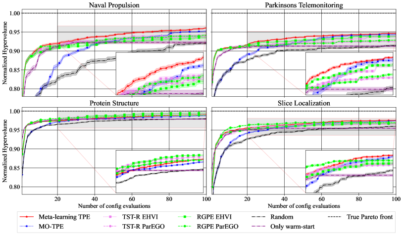
Figure 4: The normalized HV over time on four joint neural architecture search and hyperparameter optimization benchmarks (HPOlib) from HPOBench. Each method was run with $20$ different random seeds and the weak-color bands present standard error. The small inset figures in each figure are the magnified gray areas. See Appendix D for the Pareto fronts achieved by $50\%$ Watanabe (2023a) of the runs.

4.5 Validation of Modifications

To see the effect of the task kernel, we conduct an experiment using the ellipsoid function $f(\bm{x}|c)\coloneqq f(x_{1},\dots,x_{4}|c)=\sum_{d=1}^{4}5^{d-1}(x_{d}-c)^{2}$ defined on $[-5,5]^{4}$. Along with the original TPE, we optimized $f(\bm{x}|c=0)$ by meta-learning TPE using the randomly sampled $100$ observations from $f(\bm{x}|c_{\star})$ where $c^{\star}\in[0,1,\dots,4]$ (each run uses only one of $[0,1,\dots,4]$) as metadata. Furthermore, we also evaluated naïve meta-learning TPE that considers $k_{t}(t_{i},t_{j})=1/T$ for all pairs of tasks. All control parameter settings followed Section 5 except we evaluated $200$ configurations.

In Figure 2, we present the result. The top figure shows the performance curve and the bottom figure shows the weight ($k_{t}(t_{1},t_{2})\in[0,1]$) on the meta-task. As seen in the figure, the performance rank is proportional to the task similarity in the early stage of the optimizations, and thus meta-learning TPE on the dissimilar tasks performed poorly in the beginning. However, as the number of evaluations increases, the performance curves of dissimilar meta-tasks quickly approach that of TPE after $30$ evaluations where $\lfloor\log_{\eta}|\mathcal{D}^{(l)}_{1}|\rfloor$ first becomes non-zero for $\eta=2.5$. We can also see the task weight is also ordered by the similarity between the target task and the meta-task. Thanks to this effect, on the dissimilar tasks (purple, blue lines), our method starts to recover the performance of TPE from that point (see the first inset figure) and our method showed closer performance to the original TPE compared to the naïve meta-learning TPE (see the second inset figure). This result demonstrates the robustness of our method to the knowledge transfer from dissimilar meta-tasks. For similar tasks (light green, orange lines), our method accelerates at the early stage and slowly converges to the performance of TPE. Notice that since we use random search for the metadata and the observations are from the meta-learning TPE sampler, which is obviously a non-i.i.d sampler due to the iterative update nature, the top-$\gamma$-quantile in observations obtained from our method is concentrated in a subset of the true top-$\gamma$-quantile as stated in Theorem 1. It implies that the weight for meta-task is expected to decrease over time even if the target task is identical to meta-tasks.

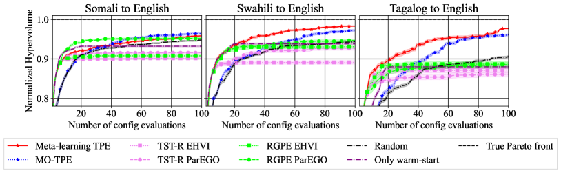
Figure 5: The normalized HV over time on NMT-Bench. Each method was run with $20$ different random seeds and the weak-color bands present standard error. See Appendix D for the Pareto fronts achieved by $50\%$ Watanabe (2023a) of the runs.

5 Experiments

5.1 Setup

In the experiments, we optimize two metrics (a validation loss or accuracy metric, and runtime) on four joint NAS & HPO benchmarks (HPOlib) Klein and Hutter (2019) in HPOBench Eggensperger et al. (2021), as well as NMT-Bench Zhang and Duh (2020). The baselines are as follows:

1. RGPE either with EHVI or ParEGO,

2. TST-R either with EHVI or ParEGO,

3. Random search,

4. Only warm-start (top-$10\%$ configurations in metadata),

5. MO-TPE Ozaki et al. (2020, 2022).

RGPE Feurer et al. (2018) and TST-R Wistuba et al. (2016) were reported to show the best average performance in a diverse set of meta-learning BO methods Feurer et al. (2018). Note that since RGPE and TST-R require a rank metric to compute the ranking loss, we used non-domination rank and crowding distance, which we use for meta-learning TPE as well. Each meta-learning method uses $100$ random configurations from the other datasets in each tabular benchmark and uses the warm-start initialization ($N_{\mathrm{init}}=5$) in Algorithm 2. Only warm-start serves as an indicator of how good the initialization could be and we can judge whether warm-start helps or the meta-learning methods help. In this setup, Algorithm 1 takes $1.0\times 10^{-4}$ seconds for a $10D$ space with $200$ observations for $5$ meta-tasks. In Appendix C, we describe more details about control parameters of each method and tabular benchmarks and discuss the effect of the control parameter $\eta$ and the number of meta-tasks on the performance.

The performance of each experiment was measured via the normalized HV. When we define the worst (maximum) and the best (minimum) values of each objective as $f^{\max}_{i},f^{\min}_{i}$ for $i\in\{1,\dots,M\}$, the normalized HV is computed as:

$$\prod_{i=1}^{M}\frac{f^{\max}_{i}-f_{i}}{f^{\max}_{i}-f^{\min}_{i}}.$$ (18)

In principle, the normalized HV is better when it is higher and the possible best value is 1, which is shown as True Pareto front. Although the normalized HV curve tells us how much each method could improve solution sets, it does not visualize how solutions distribute in the objective space (on average). Therefore, we also provide the $50\%$ empirical attainment surfaces Fonseca and Fleming (1996) in Appendix D.

5.2 Results on Real-World Tabular Benchmarks

Figure 4 shows the results on HPOlib. For all datasets, Only warm-start quickly yields results slightly worse than Random search with as many as $100$ function evaluations. This implies that the knowledge transfer surely helps at the early stage of each optimization, but each method still needs to explore better configurations. Our meta-learning TPE method shows the best performance curves except for Protein Structure; however, our method did not exhibit the best performance on Protein Structure, where its performance is still competitive. Furthermore, while we found out that Protein Structure is relatively dissimilar from the other benchmarks (as discussed in Appendix D), our method could still outperform the non-transfer MO-TPE.

Figure 5 shows the results on NMT-Bench. As in HPOlib, Only warm-start quickly yields results slightly worse than Random search with as many as $100$ function evaluations for all datasets in NMT-Bench as well. On the other hand, while RGPE and TST-R exhibit performance indistinguishable from Only warm-start in most cases, our method still improved until the end. This implies that Only warm-start is not sufficient in this task and our method could make use of the knowledge from metadata. However, our meta-learning TPE method struggled in Somali to English, which was dissimilar to the other datasets as discussed in Appendix D. Although our method did not exhibit the best performance in this case, it still recovered well with enough observations and got the best performance in the end.

6 Conclusion

In this paper, we introduced a multi-task training method for TPE and demonstrated the performance of our method. Our method measures the similarity between tasks using the intersection over union and computes the task kernel based on the similarity. As the vanilla version of this simple meta-learning method has some drawbacks, we employed the $\epsilon$-greedy algorithm and the dimension reduction method to stabilize our task kernel. In the experiment using a synthetic function, we confirmed that our task kernel correctly ranks the task similarity and our method could demonstrate robust performance over various task similarities. In the real-world experiments, we used two tabular benchmarks of expensive HPO problems. Our method could outperform other methods in most settings and still exhibit competitive performance in the worst case of dissimilar tasks. Our method’s strong performance is also backed by winning the AutoML 2022 competition on “Multiobjective Hyperparameter Optimization for Transformers”.

Appendix A Details of Meta-Learning TPE

In Appendix, $\mu$ is the Lebesgue measure defined on the search space $\mathcal{X}$ and $\mathcal{B}_{D}$ is the Borel body over $\mathbb{R}^{D}$ if not specified.

A.1 Task-Conditioned Acquisition Function

To begin with, we explain the transformation of TPE:

$$\mathrm{EI}_{f^{\gamma}}[\bm{x}|\mathcal{D}] =\int_{-\infty}^{f^{\gamma}}(f^{\gamma}-f)p(f|\bm{x})df$$ (19)

$$=\int_{-\infty}^{f^{\gamma}}(f^{\gamma}-f)\frac{p(\bm{x}|f,\mathcal{D})p(f|\mathcal{D})}{p(\bm{x}|\mathcal{D})}df$$

$$~{}~{}~{}~{}~{}(\because\mathrm{Bayes^{\prime}~{}theorem})$$

$$=\frac{p(\bm{x}|\mathcal{D}^{(l)})}{p(\bm{x}|\mathcal{D})}\underbrace{\int_{-\infty}^{f^{\gamma}}(f^{\gamma}-f)p(f|\mathcal{D})df}_{\mathrm{const~{}w.r.t.~{}}\bm{x}}~{}(\because\mathrm{Eq.}~{}(\ref{eq:l-and-g-trick}))$$

$$\propto\frac{p(\bm{x}|\mathcal{D}^{(l)})}{\gamma p(\bm{x}|\mathcal{D}^{(l)})+(1-\gamma)p(\bm{x}|\mathcal{D}^{(g)})}$$

$$~{}\biggl{(}\because p(\bm{x}|\mathcal{D})=\int_{-\infty}^{\infty}p(\bm{x}|f,\mathcal{D})p(f|\mathcal{D})df\biggr{)}.$$

In the same vein, we transform the task-conditioned AF:

$$\mathrm{EI}_{f^{\gamma}}[\bm{x}|t,\bm{D}] =\int_{-\infty}^{f^{\gamma}}(f^{\gamma}-f)p(f|\bm{x},t,\bm{D})df$$ (20)

$$=\int_{-\infty}^{f^{\gamma}}(f^{\gamma}-f)\frac{p(\bm{x},t|f,\bm{D})p(f|\bm{D})}{p(\bm{x},t|\bm{D})}df$$

$$~{}~{}~{}~{}~{}(\because\mathrm{Bayes^{\prime}~{}theorem}).$$

To further transform, we assume the conditional shift Zhang et al. (2013). In the conditional shift, we assume that all tasks have the same target PDF, i.e. $p(f|t_{i})=p(f|t_{j})$ (see Figure 6). Since TPE considers ranks of observations and ignore the scale, the optimization of $f(\bm{x})$ is equivalent to that of the quantile of $f(\bm{x})$. For this reason, the only requirement to achieve the conditional shift is to use the same quantile $\gamma$ for the split of observations $\mathcal{D}_{m}$ of all meta-tasks. In Figure 6, we visualize two functions and their quantile functions along with their target PDFs $p(f)$. As seen in the figure, the quantile functions equalize the target PDF while preserving the order of each point. Let $f$ be the quantile function (a mapping from $\mathcal{X}$ to $[0,1]$) for convenience and then we obtain the following:

$$p(\bm{x},t|f,\bm{D})\coloneqq\left\{\begin{array}[]{ll}p(\bm{x},t|\bm{D}^{(l)})&(f\leq\gamma)\\ p(\bm{x},t|\bm{D}^{(g)})&(f>\gamma)\end{array}\right.$$ (23)

where $\bm{D}^{(l)}\coloneqq\{\mathcal{D}^{(l)}_{m}\}_{m=1}^{T}$ is a set of the $\gamma$-quantile observations and the conditional shift plays a role to enable us to have a unique split point, which is at $f=\gamma$. Then we can further transform as follows:

$$\int_{-\infty}^{f^{\gamma}}(f^{\gamma}-f)\frac{p(\bm{x},t|f,\bm{D})p(f|\bm{D})}{p(\bm{x},t|\bm{D})}df$$

$$= \int_{0}^{\gamma}(\gamma-f)\frac{p(\bm{x},t|f,\bm{D})p(f|\bm{D})}{p(\bm{x},t|\bm{D})}df~{}(\because f\in[0,1])$$

$$= \frac{p(\bm{x},t|\bm{D}^{(l)})}{p(\bm{x},t|\bm{D})}\underbrace{\int_{0}^{\gamma}p(f|\bm{D})df}_{\mathrm{const~{}w.r.t.~{}}\bm{x}}$$

$$\propto \frac{p(\bm{x},t|\bm{D}^{(l)})}{\gamma p(\bm{x},t|\bm{D}^{(l)})+(1-\gamma)p(\bm{x},t|\bm{D}^{(g)})}.$$ (24)

As seen in the equations above, since TPE always ignores the improvement term $f^{\gamma}-f$, we can actually view the AF as probability of improvement (PI). Note that the equivalence of PI and EI in the TPE formulation is already reported in prior works watanabe2022ctpe,watanabe2023ctpe,song2022general. Then the conditional shift can be explained in a more straightforward way. Since PI requires the binary classification of $\mathcal{D}$ into $\mathcal{D}^{(l)}$ or $\mathcal{D}^{(g)}$, $p(f|\mathcal{D})$ just depends on our split. More specifically, if we regard $f$ as $\mathbbm{I}[f\leq f^{\gamma}]$ and then we simply get $p(f|\mathcal{D})$ as $p(f=1|\mathcal{D})=|\mathcal{D}^{(l)}|/|\mathcal{D}|=\gamma$ and $p(f=0|\mathcal{D})=|\mathcal{D}^{(g)}|/|\mathcal{D}|=1-\gamma$. For this reason, the assumption is easily satisfied as long as we fix $\gamma$ for all tasks. Note that the $\gamma$-quantile in observations is usually better, i.e. $\mathcal{D}^{(l)}\rightarrow\mathcal{X}^{\gamma^{\prime}}$ s.t. $\gamma^{\prime}<\gamma$ as stated in Theorem 1, than the true $\gamma$-quantile value $f^{\gamma}$ with a high probability when we use a non-random sampler as a non-random sampler usually performs better than random search. It implies that the quality of knowledge about top domains will be relatively low in meta-tasks if we have much more observations on the target task and our method might not be accelerated drastically although we can guarantee the conditional shift. We designed our task similarity to decay the similarity so that our method will not suffer from the knowledge dilution problem.

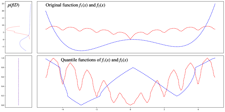
Figure 6: Examples of the quantile function. When we transform a function into a quantile function, we will get the uniform PDF. Top row: the shapes of the original functions $f_{1}(x),f_{2}(x)$ (Right) and the PDFs of each function (Left). Bottom row: the shapes of the quantile functions of $f_{1}(x),f_{2}(x)$ (Right) and the PDFs of each quantile function (Left). After the quantile transformation, the target PDFs of each function perfectly match.

A.2 Task Similarity

Since the $\gamma$-set similarity is intractable due to the unavailability of the true $\gamma$-set $\mathcal{X}^{\gamma}$, we describe how to estimate the $\gamma$-set similarity. First, we define the measure space $(\Omega,\mathcal{F},\mu_{\Omega})$ such that $\Omega\coloneqq\prod_{k=1}^{\infty}\mathcal{X}$, $\mathcal{F}$ is the minimum $\sigma$-algebra on the cylinder set of $\mathcal{B}_{\mathcal{X}}$, and $\mu_{\Omega}$ is the Lebesgue measure on $\Omega$ and define the Borel body over $\mathcal{X}$ as $\mathcal{B}_{\mathcal{X}}\coloneqq\mathcal{B}_{D}\cap\mathcal{X}$. Then, we prove the following theorem:

Theorem 2

Given a measure space $(\Omega,\mathcal{F}_{\Omega},\mu_{\Omega})$ for convergence, a measure space $(\mathcal{X},\mathcal{B}_{\mathcal{X}},\mu)$ for the probability measure $\mathbb{P}$, and a strongly-consistent estimator of the $\gamma$-set $\mathrm{PDF}$ $p\mathrm{:}~{}\mathcal{X}\rightarrow\mathbb{R}_{\geq 0}$, then the following approximation almost surely converges to the $\gamma$-set similarity:

$$\hat{s}(\mathcal{D}^{(l)}_{i},\mathcal{D}^{(l)}_{j})\coloneqq\frac{1-d_{\mathrm{tv}}(p_{i},p_{j})}{1+d_{\mathrm{tv}}(p_{i},p_{j})}\stackrel{{\scriptstyle a.s.}}{{\rightarrow}}s(\mathcal{X}^{\gamma}_{i},\mathcal{X}^{\gamma}_{j})$$ (25)

where $\stackrel{{\scriptstyle a.s.}}{{\rightarrow}}$ implies almost sure convergence with respect to the measure space $(\Omega,\mathcal{F}_{\Omega},\mu_{\Omega})$ and $d_{\mathrm{tv}}$ is the total variation distance:

$$d_{\mathrm{tv}}(p_{i},p_{j})\coloneqq\frac{1}{2}\int_{\bm{x}\in\mathcal{X}}|p(\bm{x}|\mathcal{D}^{(l)}_{i})-p(\bm{x}|\mathcal{D}^{(l)}_{j})|\mu(d\bm{x}).$$ (26)

The proof is provided in Appendix B.4.

Appendix B Proofs

B.1 Assumptions

In this paper, we assume the following:

1. Objective function $f:\mathcal{X}\rightarrow\mathbb{R}$ is Lebesgue integrable and measurable defined over the compact convex measurable subset $\mathcal{X}\subseteq\mathbb{R}^{D}$,

2. The probability measure $\mathbbm{I}[\bm{x}\in\mathcal{X}^{\gamma}]$ is Riemann integrable over $\mathcal{X}$,

3. The PDF of the probability measure $\mathbbm{I}[\bm{x}\in\mathcal{X}^{\gamma}]$ always exists, and

4. The target PDFs are identical, i.e. $p(f|t_{i})=p(f|t_{j})$ for all task pairs, while the conditional PDFs can be different, i.e. $p(\bm{x}|f,t_{i})\neq p(\bm{x}|f,t_{j})$ where $t_{i}$ for $i\in\{1,\dots,T\}$ is the symbol for the $i$-th task, respectively.

Strictly speaking, we cannot guarantee that the PDF of the probability measure $\mathbbm{I}[\bm{x}\in\mathcal{X}^{\gamma}]$ always exists; however, we formally assume that the PDF exists by considering the formal derivative of the step function as the Dirac delta function. The fourth assumption is known as conditional shift zhang2013domain. Note that a categorical parameter with $K$ categories is handled as $\mathcal{X}_{i}=[1,K]$ as in the TPE implementation bergstra2011algorithms as we do not require the continuity of $f$ with respect to hyperparameters in our theoretical analysis, this definition is valid as long as the employed kernel for categorical parameters treats different categories to be equally similar such as Aitchison kernel aitchison1976multivariate. In this definition, $x,x^{\prime}\in\mathcal{X}_{i}$ are viewed as equivalent as long as $\lfloor x\rfloor=\lfloor x^{\prime}\rfloor$ and it leads to the random sampling of each category being uniform and the Lebesgue measure of $\mathcal{X}$ to be non-zero.

B.2 Preliminaries

In this paper, we consistently use the Lebesgue integral $\int_{\bm{x}\in\mathcal{X}}g(\bm{x})\mu(d\bm{x})$ instead of the Riemann integral $\int_{\bm{x}\in\mathcal{X}}g(\bm{x})d\bm{x}$; however, $\int_{\bm{x}\in\mathcal{X}}g(\bm{x})d\bm{x}=\int_{\bm{x}\in\mathcal{X}}g(\bm{x})\mu(d\bm{x})$ holds if $g(\bm{x})$ is Riemann integrable. The only reason why we use the Lebesgue integral is that some functions in our discussion cannot be handled by the Riemann integral. Hence, we encourage readers to replace $\mu(d\bm{x})$ with $d\bm{x}$ if they are not familiar to the Lebesgue integral.

Since all definitions can easily be expanded to the MO case, we discuss the single objective case for simplicity and mention how to expand to the MO case in Appendix B.3. Throughout this paper, we use the following terms for the discussion later (see Figure 1 to get the insight):

Definition 1 ($\gamma$-quantile value)

Given a quantile $\gamma\in(0,1]$ and a measurable function $f\mathrm{:}~{}\mathcal{X}\rightarrow\mathbb{R}$, $\gamma$-quantile value $f^{\gamma}\in\mathbb{R}$ is a real number such that$\mathrm{:}$

$$f^{\gamma}\coloneqq\inf\biggl{\{}f^{\star}\in\mathbb{R}~{}\biggl{|}\int_{\bm{x}\in\mathcal{X}}\mathbbm{I}[f(\bm{x})\leq f^{\star}]\frac{\mu(d\bm{x})}{\mu(\mathcal{X})}\geq\gamma\biggr{\}}.$$ (27)

In this paper, if $\mathcal{X}$ is a countable set, we only consider discrete dimensions such that $\{\frac{k}{n}\}_{k=0}^{n}$ ($n$ can be infinity). For example, when $D=1$, we define $I_{k,n}\coloneqq[\frac{k}{n},\frac{k+1}{n})$ and $f(x)\coloneqq\sum_{k=0}^{n-1}\mathbbm{I}[x\in I_{k,n}]f(\frac{k}{n})$ (if $n\rightarrow\infty$, we will take the limit of the RHS). Then we can relax a discrete function to a continuous function, and thus we obtain the $\gamma$-quantile value as defined above.

Definition 2 ($\gamma$-set)

Given a quantile $\gamma\in(0,1]$, $\gamma$-set $\mathcal{X}^{\gamma}$ is defined as $\mathcal{X}^{\gamma}\coloneqq\{\bm{x}\in\mathcal{X}\mid f(\bm{x})\leq f^{\gamma}\}\in\mathcal{B}_{\mathcal{X}}$ where $\mathcal{B}_{\mathcal{X}}\coloneqq\mathcal{B}_{D}\cap\mathcal{X}$ is the Borel body over $\mathcal{X}$.

Definition 3 ($\gamma$-set similarity)

Given two objective functions $f_{1},f_{2}$ and $\gamma\in(0,1]$, let the $\gamma$-sets for $f_{1},f_{2}$ be $\mathcal{X}^{\gamma}_{1},\mathcal{X}^{\gamma}_{2}$. Then we define $\gamma$-set similarity $s:\mathcal{B}_{\mathcal{X}}\times\mathcal{B}_{\mathcal{X}}\rightarrow[0,1]$ between $f_{1}$ and $f_{2}$ as follows$\mathrm{:}$

$$s(\mathcal{X}^{\gamma}_{1},\mathcal{X}^{\gamma}_{2})=\frac{\mu(\mathcal{X}^{\gamma}_{1}\cap\mathcal{X}^{\gamma}_{2})}{\mu(\mathcal{X}^{\gamma}_{1}\cup\mathcal{X}^{\gamma}_{2})}.$$ (28)

Note that those definitions rely on some assumptions described in Appendix B.1.

B.3 Generalization of Tree-Structured Parzen Estimator with Multi-Objective Optimization

As mentioned in the main paper, the extension of TPE to MO settings can be easily achieved using a rank metric $R$. For this reason, we stick to the single objective setting for simplicity; however, we describe the theoretical background for the extension here. We first reformulate PI (as mentioned previously the AF of TPE is equivalent to PI Watanabe and Hutter (2022, 2023); Song et al. (2022)) using the Lebesgue integral:

$$\mathrm{Riemann~{}formulation}\!:$$ (29)

$$~{}~{}~{}~{}~{}~{}~{}~{}~{}~{}\mathbb{P}(f\leq f^{\gamma}|\bm{x},\mathcal{D})=\int_{-\infty}^{f^{\gamma}}p(f|\bm{x},\mathcal{D})df$$

$$\mathrm{Lebesgue~{}formulation}\!:$$

$$~{}~{}~{}~{}~{}~{}~{}~{}~{}~{}\mathbb{P}(f\leq f^{\gamma}|\bm{x},\mathcal{D})=\int_{\mathcal{Y}}p(f|\bm{x},\mathcal{D})\mathbbm{I}[f\in\mathcal{Y}^{\gamma}]\mu_{\mathcal{Y}}(df)$$

where $\mathcal{Y}^{\gamma}\in\mathcal{B}_{\mathcal{Y}}$ is defined as the Borel body $\mathcal{B}_{\mathcal{Y}}$ over the objective space $\mathcal{Y}$ and $\mu_{\mathcal{Y}}$ is the Lebesgue measure defined on $\mathcal{Y}$, and $\mathcal{Y}^{\gamma}$ is defined so that:

$$\gamma\coloneqq\frac{\int_{\mathcal{Y}}p(f|\bm{x},\mathcal{D})\mathbbm{I}[f\in\mathcal{Y}^{\gamma}]\mu_{\mathcal{Y}}(df)}{\int_{\mathcal{Y}}p(f|\bm{x},\mathcal{D})\mu_{\mathcal{Y}}(df)}$$ (30)

holds. For example, $\mathcal{Y}^{\gamma}=(-\infty,f^{\gamma}]$ in the 1D example and $\mathcal{Y}^{\gamma}=\{f\in\mathcal{Y}\mid R(f)\leq R(f^{\gamma})\}$ in MO cases. In MO cases, only the Lebesgue formulation could be strictly defined and we compute PI as follows:

$$\mathbb{P}(\bm{f}\preceq\bm{f}^{\gamma}|\bm{x},\mathcal{D}) \coloneqq\mathbb{P}(R(\bm{f})\leq R(\bm{f}^{\gamma})|\bm{x},\mathcal{D})$$ (31)

$$=\int_{\mathcal{Y}}p(\bm{f}|\bm{x},\mathcal{D})\mathbbm{I}[\bm{f}\in\mathcal{Y}^{\gamma}]\mu_{\mathcal{Y}}(d\bm{f})$$

where $\preceq$ is an operator such that $\bm{f}$ is equally good or better than $\bm{f}^{\gamma}$ based on a rank metric $R:\mathbb{R}^{m}\rightarrow\mathbb{R}$ for an objective vector $\bm{f}$. For example, in the single objective case, $\mathcal{Y}^{\gamma}$ is just $(-\infty,f^{\gamma}]$ and $R(f)=f$. In MO cases, we used the non-dominated rank and the crowding distance as $R$. In principle, MO settings fall back to the single objective setting after we apply $R$ to an objective vector $\bm{f}$.

B.4 Proof of Theorem 26

Throughout this section, we denote $\mathcal{D}^{(l)}_{m,N}$ as the $\mathcal{D}^{(l)}_{m}$ with the size of $N$ for notational clarity. Then we first prove the following lemma:

Lemma 1

Given the a measurable space $(\mathcal{X},\mathcal{B}_{\mathcal{X}},\mu)$, the $\gamma$-set similarity between two functions $f_{i},f_{j}$ is computed as$\mathrm{:}$

$$s(\mathcal{X}^{\gamma}_{i},\mathcal{X}^{\gamma}_{j})=\frac{1-d_{\mathrm{tv}}(p_{i},p_{j})}{1+d_{\mathrm{tv}}(p_{i},p_{j})}.$$ (32)

where $P_{i}=\mathbb{P}[\bm{x}\in\mathcal{X}^{\gamma}_{i}],P_{j}=\mathbb{P}[\bm{x}\in\mathcal{X}^{\gamma}_{j}]$ are the probability measure of $p_{i}=p(\bm{x}|\mathcal{X}^{\gamma}_{i}),p_{j}=p(\bm{x}|\mathcal{X}^{\gamma}_{j})$ and

$$d_{\mathrm{tv}}(p_{i},p_{j}) =\frac{1}{2}\|P_{i}-P_{j}\|_{1}$$ (33)

$$=\frac{1}{2}\int_{\bm{x}\in\mathcal{X}}|p(\bm{x}|\mathcal{X}^{\gamma}_{i})-p(\bm{x}|\mathcal{X}^{\gamma}_{j})|\mu(d\bm{x})$$

is the total variation distance.

Note that we used the Scheffe’s lemma tsybakovintroduction for the transformation in Eq. (33).

Proof 1

Since $\bm{x}$ is either in or not in $\mathcal{X}^{\gamma}$ and $\mathcal{X}^{\gamma}$ is fixed, the probability measure takes either $0$ or $1$. For this reason, the following holds$\mathrm{:}$

$$\mathbbm{I}[\bm{x}\in\mathcal{X}^{\gamma}_{i}\cap\mathcal{X}^{\gamma}_{j}] =\mathbb{P}[\bm{x}\in\mathcal{X}^{\gamma}_{i}\cap\mathcal{X}^{\gamma}_{j}]$$ (34)

$$=\mathbb{P}[\bm{x}\in\mathcal{X}^{\gamma}_{i}]\wedge\mathbb{P}[\bm{x}\in\mathcal{X}^{\gamma}_{j}],$$

$$\mathbbm{I}[\bm{x}\in\mathcal{X}^{\gamma}_{i}\cup\mathcal{X}^{\gamma}_{j}] =\mathbb{P}[\bm{x}\in\mathcal{X}^{\gamma}_{i}\cup\mathcal{X}^{\gamma}_{j}]$$

$$=\mathbb{P}[\bm{x}\in\mathcal{X}^{\gamma}_{i}]\vee\mathbb{P}[\bm{x}\in\mathcal{X}^{\gamma}_{j}]$$

where $\wedge,\vee$ are equivalent to the $\min$ and $\max$ operator, respectively. Notice that $\mathcal{X}^{\gamma}_{1},\mathcal{X}^{\gamma}_{2}$ must be measurable sets so that the equation above is valid. It leads to the following equations$\mathrm{:}$

$$\mu(\mathcal{X}^{\gamma}_{i}\cap\mathcal{X}^{\gamma}_{j}) =\int_{\bm{x}\in\mathcal{X}}\mathbb{P}[\bm{x}\in\mathcal{X}^{\gamma}_{i}\cap\mathcal{X}^{\gamma}_{j}]\mu(d\bm{x}),$$ (35)

$$\mu(\mathcal{X}^{\gamma}_{i}\cup\mathcal{X}^{\gamma}_{j}) =\int_{\bm{x}\in\mathcal{X}}\mathbb{P}[\bm{x}\in\mathcal{X}^{\gamma}_{i}\cup\mathcal{X}^{\gamma}_{j}]\mu(d\bm{x}).$$

Using $\mathrm{Eqs.~{}(\ref{appx:proof:eq:prob-measure-and-operators}),(\ref{appx:proof:eq:volume-vs-prob-measure})}$, we obtain the following equation$\mathrm{:}$

$$s(\mathcal{X}^{\gamma}_{i},\mathcal{X}^{\gamma}_{j}) =\frac{\int_{\bm{x}\in\mathcal{X}}\mathbb{P}[\bm{x}\in\mathcal{X}^{\gamma}_{i}]\wedge\mathbb{P}[\bm{x}\in\mathcal{X}^{\gamma}_{j}]\mu(d\bm{x})}{\int_{\bm{x}\in\mathcal{X}}\mathbb{P}[\bm{x}\in\mathcal{X}^{\gamma}_{i}]\vee\mathbb{P}[\bm{x}\in\mathcal{X}^{\gamma}_{j}]\mu(d\bm{x})}$$ (36)

$$=\frac{1-d_{\mathrm{tv}}(p_{i},p_{j})}{1+d_{\mathrm{tv}}(p_{i},p_{j})}.$$

This completes the proof.

Then we need to prove the following lemma as well:

Lemma 2

Given the assumptions above and the measurable spaces defined in the statement of $\mathrm{Theorem}~{}\ref{main:methods:theorem:convergence-of-gamma-similarity}$, the following holds under the assumption (denote $\mathrm{Assumption~{}(\star)}$) of $\exists\epsilon>0,\lim_{N\rightarrow\infty}\|(p(\bm{x}|\mathcal{D}^{(l)}_{m,N})-\mathbbm{I}[\bm{x}\in\mathcal{X}^{\gamma}_{m}]/\mu(\mathcal{X}^{\gamma}_{m}))\mathbbm{I}[\bm{x}\in\epsilon\bm{B}_{N}]\|_{\infty}=0$ for all $m$ where $\bm{B}_{N}\subseteq\mathbb{R}^{D}$ is a ball with radius $N$ centered at $\bm{0}\mathrm{:}$

$$\int_{\bm{x}\in\mathcal{X}}|p(\bm{x}|\mathcal{D}^{(l)}_{i,N})-p(\bm{x}|\mathcal{D}^{(l)}_{j,N})|\mu(d\bm{x})$$ (37)

$$\stackrel{{\scriptstyle a.s.}}{{\rightarrow}}\int_{\bm{x}\in\mathcal{X}}\biggl{|}\frac{\mathbbm{I}[\bm{x}\in\mathcal{X}^{\gamma}_{i}]}{\mu(\mathcal{X}^{\gamma}_{i})}-\frac{\mathbbm{I}[\bm{x}\in\mathcal{X}^{\gamma}_{j}]}{\mu(\mathcal{X}^{\gamma}_{j})}\biggr{|}\mu(d\bm{x})~{}(N\rightarrow\infty).$$

Proof 2

From the assumption of the strongly-consistent estimator, the following uniform convergence holds wied2012consistency for all $m\in\{1,\dots,T\}$ and $\forall\epsilon>0$ at each point of continuity $\bm{x}$ of $\mathbbm{I}[\bm{x}\in\mathcal{X}^{\gamma}_{m}]\mathrm{:}$

$$p(\bm{x}|\mathcal{D}^{(l)}_{m,N})\stackrel{{\scriptstyle a.s.}}{{\rightarrow}}\frac{\mathbbm{I}[\bm{x}\in\mathcal{X}^{\gamma}_{m}]}{\mu(\mathcal{X}^{\gamma}_{m})}~{}(N\rightarrow\infty).$$ (38)

Note that the uniform convergence almost surely happens with respect to an arbitrary sample from $\Omega$ that achieves the strong consistency of $\mathrm{KDE}$. Therefore, the following holds using the continuous mapping theorem$\mathrm{:}$

$$|p(\bm{x}|\mathcal{D}^{(l)}_{i,N})-p(\bm{x}|\mathcal{D}^{(l)}_{j,N})|$$ (39)

$$\stackrel{{\scriptstyle a.s.}}{{\rightarrow}}\biggl{|}\frac{\mathbbm{I}[\bm{x}\in\mathcal{X}^{\gamma}_{i}]}{\mu(\mathcal{X}^{\gamma}_{i})}-\frac{\mathbbm{I}[\bm{x}\in\mathcal{X}^{\gamma}_{j}]}{\mu(\mathcal{X}^{\gamma}_{j})}\biggr{|}~{}(N\rightarrow\infty).$$

From the assumptions, all functions are defined over the compact convex measurable subset $\mathcal{X}\subseteq\mathbb{R}^{D}$ and all convergences in this proof are uniform and almost sure; therefore, we obtain the following result based on $\mathrm{Theorem~{}7.16}$ of rudin1976principles$\mathrm{:}$

$$\lim_{N\rightarrow\infty}\int_{\bm{x}\in\mathcal{X}}|p(\bm{x}|\mathcal{D}^{(l)}_{i,N})-p(\bm{x}|\mathcal{D}^{(l)}_{j,N})|\mu(d\bm{x})$$ (40)

$$=\int_{\bm{x}\in\mathcal{X}}\lim_{N\rightarrow\infty}|p(\bm{x}|\mathcal{D}^{(l)}_{i,N})-p(\bm{x}|\mathcal{D}^{(l)}_{j,N})|\mu(d\bm{x})$$

$$\stackrel{{\scriptstyle a.s.}}{{\rightarrow}}\int_{\bm{x}\in\mathcal{X}}\biggl{|}\frac{\mathbbm{I}[\bm{x}\in\mathcal{X}^{\gamma}_{i}]}{\mu(\mathcal{X}^{\gamma}_{i})}-\frac{\mathbbm{I}[\bm{x}\in\mathcal{X}^{\gamma}_{j}]}{\mu(\mathcal{X}^{\gamma}_{j})}\biggr{|}\mu(d\bm{x}).$$

Note that the last transformation requires $\mathrm{Assumption~{}(\star)}$ to be true with the probability of $1$. This completes the proof.

From Eq. (36) in Lemma 1, Eq. (37) in Lemma 37 and the continuous mapping theorem, the statement of Theorem 26 is proved and this completes the proof.

B.5 Proof of Theorem 1

Theorem 3

If we use the $\epsilon$-greedy policy ($\epsilon\in(0,1)$) for $\mathrm{TPE}$ to choose the next candidate $\bm{x}$ for a noise-free objective function $f(\bm{x})$ defined on search space $\mathcal{X}$ with at most a countable number of configurations, and we use a $\mathrm{KDE}$ whose distribution converges to the empirical distribution as the number of samples goes to infinity, then a set of the top-$\gamma$-quantile observations $\mathcal{D}^{(l)}_{1}$ is almost surely a subset of $\mathcal{X}^{\gamma}$.

Proof 3

First, we define a function defined on at most countable set as $f_{k}(\bm{x})\coloneqq f(k\lfloor\bm{x}/k\rfloor)$ so that we can still define the $\mathrm{PDF}$ $p(\bm{x}|f)$ on $\mathcal{X}$. In this proof, we assume $\mathcal{X}=[0,1]^{D}$ and we choose the next configuration from $\mathcal{X}_{(k)}\coloneqq\{0,1/k,\dots,(k-1)/k,1\}^{D}$. We first prove the finite case and then take $k\rightarrow\infty$ to prove the countable case. First, we list the facts that are immediately drawn from the assumptions$\mathrm{:}$

1. The $\mathrm{KDE}$ with a set of control parameters $\bm{\alpha}_{N}$ at the $N$-th iteration converges to the empirical distribution, i.e.

   $$\lim_{N\rightarrow\infty}\frac{1}{N}\sum_{n^{\prime}=1}^{N}k(\bm{x},\bm{x}_{n^{\prime}}|\bm{\alpha}_{N})\rightarrow\lim_{N\rightarrow\infty}\frac{1}{N}\sum_{n^{\prime}=1}^{N}\delta(\bm{x},\bm{x}_{n^{\prime}}),$$ (41)

2. Due to the random part in the $\epsilon$-greedy policy, we almost surely covers all possible configurations $\bm{x}\in\mathcal{X}_{(k)}$ with a sufficiently large number of samples,

3. $\forall\bm{x}\in\mathcal{D}^{(l)}_{N},p(\bm{x}|\mathcal{D}^{(l)}_{N})>0$,

4. $\forall\epsilon^{\prime}>0,\exists N>0,\forall\bm{x}\notin\mathcal{D}^{(l)}_{N},p(\bm{x}|\mathcal{D}^{(l)}_{N})<\epsilon^{\prime}$,

5. $\forall\bm{x}\in\mathcal{D}^{(g)}_{N},p(\bm{x}|\mathcal{D}^{(g)}_{N})>0$, and

6. $\forall\epsilon^{\prime}>0,\exists N>0,\forall\bm{x}\notin\mathcal{D}^{(g)}_{N},p(\bm{x}|\mathcal{D}^{(g)}_{N})<\epsilon^{\prime}$.

Since $\forall\epsilon^{\prime}>0,\exists N>0,\mathcal{D}^{(l)}_{N}\stackrel{{\scriptstyle a.s.}}{{\subseteq}}\mathcal{X}_{(k)}^{\gamma+\epsilon^{\prime}}$ holds from the weak law of large numbers if $\epsilon=1$, the main strategy of this proof is to show “the probability of drawing $\bm{x}\in\mathcal{X}^{\gamma}_{(k)}$ is higher than $\gamma$ as $N$ goes to infinity”. We use the following fact in the $\mathrm{AF}$ of the $\mathrm{TPE}$ formulation watanabe2022ctpe,watanabe2023ctpe$\mathrm{:}$

$$\mathrm{EI}_{f^{\gamma}}[\bm{x}]\propto\mathrm{PI}_{f^{\gamma}}[\bm{x}]=\frac{\gamma p(\bm{x}|\mathcal{D}^{(l)})}{\gamma p(\bm{x}|\mathcal{D}^{(l)})+(1-\gamma)p(\bm{x}|\mathcal{D}^{(g)})}.$$ (42)

Since we use the $\epsilon$-greedy algorithm, $\lim_{N\rightarrow\infty}p(\bm{x}|\mathcal{D}^{(l)}_{N})\stackrel{{\scriptstyle a.s.}}{{\geq}}\epsilon/(k+1)^{D}$ and $\lim_{N\rightarrow\infty}p(\bm{x}|\mathcal{D}^{(g)}_{N})\stackrel{{\scriptstyle a.s.}}{{\geq}}\epsilon/(k+1)^{D}$ hold for all $\bm{x}\in\mathcal{X}_{(k)}$. It implies that $p(\bm{x}|\mathcal{D}^{(l)}_{N})$ and $p(\bm{x}|\mathcal{D}^{(g)}_{N})$ dominate each other if $\bm{x}\notin\mathcal{D}^{(g)}_{N}$ or $\bm{x}\notin\mathcal{D}^{(l)}_{N}$, respectively. Therefore, when we take a sufficiently large $N$, the following holds$\mathrm{:}$

1. $\forall\epsilon^{\prime},\exists N>0,\forall\bm{x}\notin\mathcal{D}^{(g)}_{N},|\mathrm{PI}_{f^{\gamma}}[\bm{x}]-1|<\epsilon^{\prime}$, and

2. $\forall\epsilon^{\prime},\exists N>0,\forall\bm{x}\notin\mathcal{D}^{(l)}_{N},\mathrm{PI}_{f^{\gamma}}[\bm{x}]<\epsilon^{\prime}$.

Notice that we cannot determine $\mathrm{PI}_{f^{\gamma}}[\bm{x}]$ for $\bm{x}\in\mathcal{D}^{(l)}_{N}\cap\mathcal{D}^{(g)}_{N}$ and we assume that a sufficiently large $N$ allows $\mathrm{TPE}$ to cover all possible configurations at least once. For this reason, the greedy algorithm always picks a configuration $\bm{x}\in\mathcal{D}^{(l)}_{N}$. Since $\mathcal{D}^{(l)}_{N}$ is determined based on the objective function $f_{k}$ and all possible configurations are covered due to the random policy, either of the following is satisfied$\mathrm{:}$

1. $\mathcal{D}^{(l)}_{N}\subseteq\mathcal{X}_{(k)}^{\gamma^{\prime}}$ such that $\gamma^{\prime}\leq\gamma$, or

2. $\mathcal{X}_{(k)}^{\gamma}\subseteq\mathcal{D}^{(l)}_{N}$.

For the first case, we obtain $\bm{x}\in\mathcal{X}^{\gamma}_{(k)}$ with the probability of $1$ and we obtain $\bm{x}\in\mathcal{X}^{\gamma}_{(k)}$ with the probability of $\gamma(k+1)^{D}/|\mathrm{set}(\mathcal{D}^{(l)}_{N})|>\gamma$ for the second case. Since the random policy obviously picks a configuration $\bm{x}\in\mathcal{X}^{\gamma}_{(k)}$ with the probability of $\gamma$, the probability of drawing $\bm{x}\in\mathcal{X}^{\gamma}_{(k)}$ is larger than $\epsilon\gamma+(1-\epsilon)\min(1,\gamma(k+1)^{D}/|\mathrm{set}(\mathcal{D}^{(l)}_{N})|)>\gamma$; therefore, it concludes that $\mathcal{D}^{(l)}_{N}\stackrel{{\scriptstyle a.s.}}{{\subseteq}}\mathcal{X}^{\gamma}_{(k)}$ and this completes the proof for the finite case. The countable case is completed by $n\rightarrow\infty$.

Using this lemma, we prove the theorem of interest, i.e. Theorem 1.

Proof 4

Let $\{\mathcal{D}_{m}\}_{m=1}^{T}$ with $|\mathcal{D}_{1}|=N$ be $\bm{D}_{N}$ and the splits of $\bm{D}_{N}$ be $\bm{D}^{(l)}_{N}$ and $\bm{D}^{(g)}_{N}$. We also define the observations of the target task with the size of $N$ as $\mathcal{D}_{N}$ for the simplicity. Notice that we assume that $N$ is sufficiently large to cover all possible configurations as in the proof of $\mathrm{Theorem~{}\ref{appendix:proofs:theorem:tpe-with-eps-greedy-converges-to-gamma-set}}$. Due to the fact that the limit of the joint $\mathrm{PDF}$ converges to the original $\mathrm{PDF}$, i.e. $\lim_{N\rightarrow\infty}p(\bm{x},t|\bm{D}^{(l)}_{N})=p(\bm{x}|\mathcal{D}^{(l)}_{N})$ and $\lim_{N\rightarrow\infty}p(\bm{x},t|\bm{D}^{(g)}_{N})=p(\bm{x}|\mathcal{D}^{(g)}_{N})$, the following holds$\mathrm{:}$

$$\mathrm{Property}~{}(1).$$

$$~{}~{}~{}~{}~{}\exists N>0,\forall\bm{x}\in\mathcal{D}^{(l)}_{N},p(\bm{x},t|\bm{D}^{(l)}_{N})>0,$$

$$\mathrm{Property}~{}(2).$$

$$~{}~{}~{}~{}~{}\forall\epsilon^{\prime}>0,\exists N>0,\forall\bm{x}\in\mathcal{D}^{(l)}_{N}\setminus\mathcal{D}^{(g)}_{N},p(\bm{x},t|\bm{D}^{(g)}_{N})<\epsilon^{\prime},$$

$$\mathrm{Property}~{}(3).$$

$$~{}~{}~{}~{}~{}\exists N>0,\forall\bm{x}\in\mathcal{D}^{(g)}_{N},p(\bm{x},t|\bm{D}^{(g)}_{N})>0,$$

$$\mathrm{Property}~{}(4).$$

$$~{}~{}~{}~{}~{}\forall\epsilon^{\prime}>0,\exists N>0,\forall\bm{x}\in\mathcal{D}^{(g)}_{N}\setminus\mathcal{D}^{(l)}_{N},p(\bm{x},t|\bm{D}^{(l)}_{N})<\epsilon^{\prime}.$$

From $\mathrm{Properties~{}(1)}$ and $\mathrm{(2)}$, the $\mathrm{AF}$ converges to $1$ if $\bm{x}\in\mathcal{D}^{(l)}_{N}\setminus\mathcal{D}^{(g)}_{N},N\rightarrow\infty$. From $\mathrm{Properties~{}(3)}$ and $\mathrm{(4)}$, the $\mathrm{AF}$ converges to 0 if $\bm{x}\in\mathcal{D}^{(g)}_{N}\setminus\mathcal{D}^{(l)}_{N},N\rightarrow\infty$. Furthermore, the $\mathrm{AF}$ may take non-zero if $\forall\bm{x}\in\mathcal{D}^{(l)}_{N}\cap\mathcal{D}^{(g)}_{N}$. Since those conditions are the same for $\mathrm{Theorem~{}\ref{appendix:proofs:theorem:tpe-with-eps-greedy-converges-to-gamma-set}}$, the same discussion applies to this theorem, and thus this completes the proof.

B.6 Proof of Proposition 2

We first define $\mu_{\mathcal{X}}$ as the the Lebesgue measure on $\mathcal{X}$, $\mu_{d}$ as the Lebesgue measure on $\mathcal{X}_{d}$, and $\mu_{-d}$ as the Lebesgue measure on $\mathcal{X}_{-d}$. Then we formally define the trivial dimensions:

Definition 4 (Trivial dimension)

Given a quantile $\gamma\in(0,1]$ and a measure space $(\mathcal{X}_{d},\mathcal{B}_{d}\cap\mathcal{X}_{d},\mu_{d})$, the $d$-th dimension is trivial if $\mathbb{P}[\bm{x}\in\mathcal{X}^{\gamma}|\bm{x}_{-d}]\in\{0,1\}$ where $\bm{x}_{-d}$ is $\bm{x}$ without the $d$-th dimension and $\mathcal{X}_{d}$ is the domain of the $d$-th dimension.

The definition implies the $d$-th dimension is trivial if and only if the binary function $b(\bm{x}|\mathcal{X}^{\gamma},\bm{x}_{-d})\coloneqq\mathbbm{I}[\bm{x}\in\mathcal{X}^{\gamma}|\bm{x}_{-d}]$ does not change almost everywhere ($\mu_{d}$-a.e.) due to the variation in the $d$-th dimension when the other dimensions are fixed where we define $b(\bm{x}|\mathcal{X}^{\gamma},\bm{x}_{-d})$ as $b(\bm{x}|\mathcal{X}^{\gamma})$ such that each element, except for the $d$-th dimension, of $\bm{x}$ is fixed to $\bm{x}_{-d}$. Note that trivial dimension is a stronger concept than less important dimension in f-ANOVA. More specifically, f-ANOVA computes the marginal variance of each dimension and judges important dimensions based on the variance; however, zero variance, which implies the dimension is not important, does not guarantee that such a dimension is trivial. For example, $f(x,y)=\mathrm{sign}(x)\sin y$ leads to zero variance in both dimensions, but both dimensions obviously change the function values.

Then we prove Proposition 2.

Proof 5

From the definition of the trivial dimension, the following holds almost surely for $x_{d}\in\mathcal{X}_{d}$ when we assume the $d$-th dimension is trivial$\mathrm{:}$

$$\int_{\bm{x}_{-d}\in\mathcal{X}_{-d}}b(\bm{x}|\mathcal{X}^{\gamma},\bm{x}_{-d})\mu_{-d}(d\bm{x}_{-d})=\frac{\mu_{\mathcal{X}}(\mathcal{X}^{\gamma})}{\mu_{d}(\mathcal{X}_{d})}\biggl{|}_{x_{d}}~{}\mu_{d}\text{-}a.e.,$$ (43)

where $\mid_{x_{d}}$ means that the $d$-th dimension in $\bm{x}$ is $x_{d}$. Additionally, as the $d$-th dimension of two tasks are trivial, we obtain the following for $\forall\bm{x}_{-d}\in\mathcal{X}_{-d}\mathrm{:}$

$$b(\bm{x}|\mathcal{X}^{\gamma}_{1}\cap\mathcal{X}^{\gamma}_{2},\bm{x}_{-d}) =\min(b(\bm{x}|\mathcal{X}^{\gamma}_{1},\bm{x}_{-d}),b(\bm{x}|\mathcal{X}^{\gamma}_{2},\bm{x}_{-d})),$$ (44)

$$b(\bm{x}|\mathcal{X}^{\gamma}_{1}\cup\mathcal{X}^{\gamma}_{2},\bm{x}_{-d}) =\max(b(\bm{x}|\mathcal{X}^{\gamma}_{1},\bm{x}_{-d}),b(\bm{x}|\mathcal{X}^{\gamma}_{2},\bm{x}_{-d}))$$

where $\mathcal{X}^{\gamma}_{1},\mathcal{X}^{\gamma}_{2}$ are the $\gamma$-sets of tasks 1, 2. As both $b(\bm{x}|\mathcal{X}^{\gamma}_{1},\bm{x}_{-d}),b(\bm{x}|\mathcal{X}^{\gamma}_{2},\bm{x}_{-d})$ are also almost everywhere $0$ or $1$ ($\mu_{d}$-a.e.), $b(\bm{x}|\mathcal{X}^{\gamma}_{1}\cup\mathcal{X}^{\gamma}_{2},\bm{x}_{-d}),b(\bm{x}|\mathcal{X}^{\gamma}_{1}\cap\mathcal{X}^{\gamma}_{2},\bm{x}_{-d})$ are almost everywhere $0$ or $1$. Therefore, we obtain$\mathrm{:}$

$$\int_{\bm{x}_{-d}\in\mathcal{X}_{-d}}b(\bm{x}|\mathcal{X}^{\gamma}_{1}\cap\mathcal{X}^{\gamma}_{2},\bm{x}_{-d})\mu_{-d}(d\bm{x}_{-d})$$ (45)

$$~{}~{}~{}~{}~{}=\frac{\mu_{\mathcal{X}}(\mathcal{X}^{\gamma}_{1}\cap\mathcal{X}^{\gamma}_{2})}{\mu_{d}(\mathcal{X}_{d})}\biggl{|}_{x_{d}}~{}\mu_{d}\text{-}a.e.,$$

$$\int_{\bm{x}_{-d}\in\mathcal{X}_{-d}}b(\bm{x}|\mathcal{X}^{\gamma}_{1}\cup\mathcal{X}^{\gamma}_{2},\bm{x}_{-d})\mu_{-d}(d\bm{x}_{-d})$$

$$~{}~{}~{}~{}~{}=\frac{\mu_{\mathcal{X}}(\mathcal{X}^{\gamma}_{1}\cup\mathcal{X}^{\gamma}_{2})}{\mu_{d}(\mathcal{X}_{d})}\biggl{|}_{x_{d}}~{}\mu_{d}\text{-}a.e..$$

Using these results, the following holds$\mathrm{:}$

$$s(\mathcal{X}^{\gamma}_{1},\mathcal{X}^{\gamma}_{2}) =\frac{\mu_{\mathcal{X}}(\mathcal{X}^{\gamma}_{1}\cap\mathcal{X}^{\gamma}_{2})}{\mu_{\mathcal{X}}(\mathcal{X}^{\gamma}_{1}\cup\mathcal{X}^{\gamma}_{2})}$$ (46)

$$=\frac{\int_{\bm{x}_{-d}\in\mathcal{X}_{-d}}b(\bm{x}|\mathcal{X}^{\gamma}_{1}\cap\mathcal{X}^{\gamma}_{2},\bm{x}_{-d})\mu_{-d}(d\bm{x}_{-d})}{\int_{\bm{x}_{-d}\in\mathcal{X}_{-d}}b(\bm{x}|\mathcal{X}^{\gamma}_{1}\cup\mathcal{X}^{\gamma}_{2},\bm{x}_{-d})\mu_{-d}(d\bm{x}_{-d})}$$

$$=\frac{\int_{\bm{x}\in\mathcal{X}}b(\bm{x}|\mathcal{X}^{\gamma}_{1}\cap\mathcal{X}^{\gamma}_{2})\mu_{\mathcal{X}}(d\bm{x})}{\int_{\bm{x}\in\mathcal{X}}b(\bm{x}|\mathcal{X}^{\gamma}_{1}\cup\mathcal{X}^{\gamma}_{2})\mu_{\mathcal{X}}(d\bm{x})}$$

where the last transformation used $\mathrm{Eq.~{}(\ref{appx:proofs:eq:intersec-union-is-const})}$ and this completes the proof.

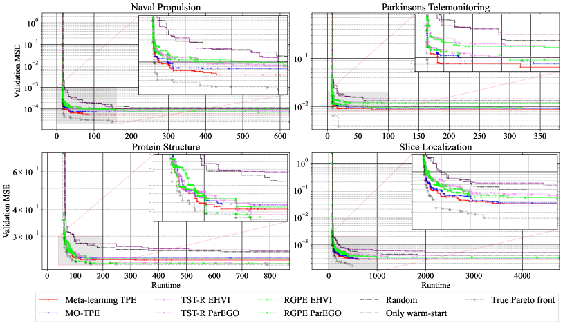
Figure 7: The $50\%$ empirical attainment surfaces watanabe2023pareto of each method over $20$ different random seeds on HPOlib. The objectives are to minimize runtime and validation MSE.

Figure 8: The $50\%$ empirical attainment surfaces watanabe2023pareto of each method over $20$ different random seeds on NMT-Bench. The objectives are to minimize runtime and maximize BLEU.

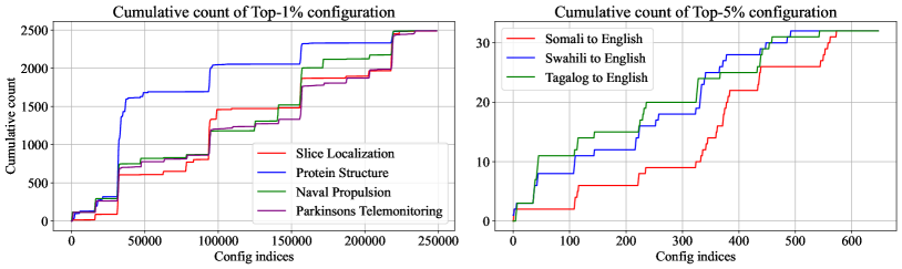
Figure 9: The cumulative count of top-$1\%$ on HPOlib (Left) and top-$5\%$ on NMT-Bench (Right) over configuration indices. Although subsequent indices do not necessarily imply that those configurations are close in the search space, each index identifies the same configuration for each dataset, and thus we can see trends by tracking the variations of each curve.

Appendix C Details of Experiments

Table 1: The search space of HPOlib. All tasks have the same search space by default. Each benchmark has performance metrics of $62208$ possible configurations with $4$ random seeds.

Hyperparameter	Choices
Number of units 1	{$2^{4},2^{5},2^{6},2^{7},2^{8},2^{9}$}
Number of units 2	{$2^{4},2^{5},2^{6},2^{7},2^{8},2^{9}$}
Dropout rate 1	{$0.0,0.3,0.6$}
Dropout rate 2	{$0.0,0.3,0.6$}
Activation function 1	{ReLU, tanh}
Activation function 2	{ReLU, tanh}
Batch size	{$2^{3},2^{4},2^{5},2^{6}$}
Learning rate scheduler	{cosine, constant}
Initial learning rate	{$5$e-$4,1$e-$3,5$e-$3,1$e-$2,5$e-$2,1$e-$1$}

Table 2: The search space of NMT-Bench. To make the search spaces for all tasks identical, we reduced the choices of “Number of layers” in the “Swahili to English” dataset. Each benchmark has performance metrics of $648$ possible configurations with $1$ random seed.

Hyperparameter	Choices
Number of BPE symbols ($\times 10^{3}$)	{$2^{0},2^{1},2^{2},2^{3},2^{4},2^{5}$}
Number of layers	{$1,2,4$}
Embedding size	{$2^{8},2^{9},2^{10}$}
Number of hidden units in each layer	{$2^{10},2^{11}$}
Number of heads in self-attention	{$2^{3},2^{4}$}
Initial learning rate ($\times 10^{-4}$)	{$3,6,10$}

C.1 Dataset Description

In the experiments, we used the following tabular benchmarks:

1. HPOlib (Slice Localization, Naval Propulsion, Parkinsons Telemonitoring, Protein Structure) klein2019tabular, and

2. NMT-Bench (Somali to English, Swahili to English, Tagalog to English) zhang2020reproducible.

The search spaces for each benchmark are presented in Tables 1, 2.

HPOlib is an HPO tabular benchmark for neural networks on regression tasks. This benchmark has four regression tasks and provides the number of parameters, runtime, and training and validation mean squared error (MSE) for each configuration. In the experiments, we optimized validation MSE and runtime.

NMT-Bench is an HPO tabular benchmark for neural machine translation (NMT) and we optimize hyperparameters of transformer. This benchmark provides three tasks: NMT for Somali to English, Swahili to English, and Tagalog to English. Since the original search space of “Swahili to English” is slightly different from the others, we reduced its search space to be identical to the others. In the experiments, we optimized translation accuracy (BLEU) papineni2002bleu and decoding speed. Note that as mentioned in Footnote 7 in the original paper zhang2020reproducible, some hyperparameters do not have both BLEU and decoding speed due to training failures; therefore, we pad the worst possible values for such cases.

C.2 Details of Optimization Methods

C.2.1 Baseline Methods

In the experiments, we used the following:

1. MO-TPE ozaki2022multiobjective,

2. Random search bergstra2012random,

3. TST-R wistuba2016two, and

4. RGPE feurer2018practical.

Note that since TST-R and RGPE are introduced as meta-learning methods for single-objective optimization problems, we extended them to MO settings using either ParEGO knowles2006parego or EHVI emmerich2011hypervolume. Since both extensions require only ranking loss between configurations, we defined the ranking of each configuration using the non-dominated rank and crowding distance as in NSGA-II deb2002fast. Although TST-R and RGPE implementations were provided in https://github.com/automl/transfer-hpo-framework, since the implementations are based on SMAC3 , which does not support EHVI, we re-implemented RGPE and TST-R using BoTorch . Our BoTorch implementations are also available in https://github.com/nabenabe0928/meta-learn-tpe. We chose $\gamma=0.1$ for MO-TPE by following the original paper ozaki2020multiobjective and modified the tie-break method from HSSP to crowding distance as TST-R and RGPE also use crowding distance for tie-breaking in our experiments. Furthermore, we employed multivariate kernel to improve the performance of TPE falkner2018bohb.

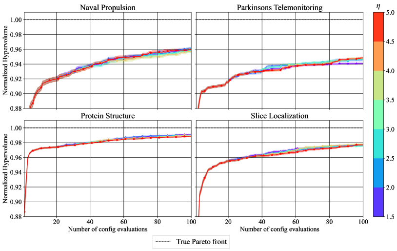
Figure 10: The ablation study of $\eta$ in our method by the normalized HV over time on four joint neural architecture search and hyperparameter optimization benchmarks (HPOlib) from HPOBench. Each method was run with $20$ different random seeds and the weak-color bands present standard error.

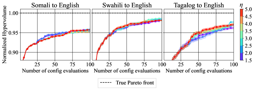
Figure 11: The ablation study of $\eta$ in our method by the normalized HV over time on NMT-Bench. Each method was run with $20$ different random seeds and the weak-color bands present standard error.

C.2.2 Settings of Meta-Learning TPE

As seen in Algorithm 2, meta-learning TPE has several control parameters:

1. (TPE) the number of initial samples $N_{\mathrm{init}}$,

2. (TPE) the number of candidates for each iteration $N_{s}$,

3. (TPE) the quantile for the observation split $\gamma$,

4. (New) dimension reduction factor $\eta$,

5. (New) sample size of Monte-Carlo sampling for the task similarity approximation $S$, and

6. (New) the ratio of random sampling in the $\epsilon$-greedy algorithm $\epsilon$.

Note that (TPE) means the parameters already existed from the original version and (New) means the parameters added in our proposition. Since the original TPE paper bergstra2011algorithms,bergstra2013making uses $5\%$ of total evaluations for the initialization and $100$ candidates for each iteration, we set $N_{\mathrm{init}}=5$ and $\epsilon=0.05$ in our experiments and used $N_{s}=100$. $\gamma=0.1$ followed the original MO-TPE ozaki2020multiobjective. For the other parameters, we used $S=1000$ and $\eta=5/2$. Note that when $S=1000$, it does not take a second to compute the similarity even with $N_{m}=10^{4}$ due to the time complexity of $O(S\max_{m\in\{1,\dots,T\}}N_{m})$. The ablation study of $\eta$ is available in the next section. Furthermore, we employed multivariate kernel as in prior works falkner2018bohb,watanabe2023ctpe and used crowding distance to tie-break non-dominated rank as mentioned in the previous section.

C.2.3 Ablation Study of $\eta$

Figures 10 and 11 show the ablation study of our method. Intuitively, when $\eta$ is low, more dimensions will be used and the similarity decay will be quicker, and thus low $\eta$ is supposed to be disadvantageous for similar task transfer. However, our method exhibits almost indistinguishable performance except for Parkinsons Telemonitoring with $\eta=1.5$. It implies that our method is robust to the choice of the control parameter $\eta$.

Figure 12: The effect of the number of tasks (Top left: $c=0$, Top right: $c=1$, Bottom left: $c=2$, Bottom right: $c=3$. A smaller $c$ implies that the target task and the meta-tasks are more similar.) on the performance of meta-learning TPE. $T$ is the number of meta-tasks to use and $T=0$ is the vanilla TPE. Each setting was run with 20 different random seeds and the weak-color bands present standard error.

C.2.4 Effect of Number of Tasks

To see the effect of the number of tasks, we tested our meta-learning TPE with different numbers of meta-tasks on different similarities of the target function. In this experiment, we used the $10D$ ellipsoid function $f(\bm{x}|c)=\sum_{d=1}^{10}5^{d-1}(x_{d}-c)^{2}$ defined on $[-5,5]^{10}$ and used $f(\bm{x}|c=0)$ as the target task. Since the contributions that meta-learning can make depend on the meta-tasks to use, we fixed a meta-task and used the same meta-task for all the meta-tasks. For example, when we use $4$ meta-tasks, we first fixed $c$ to a certain value, e.g. $c=1$, and then we used $c=1$ for all four tasks. In this way, we can avoid the similarity difference between different numbers of meta-tasks. We collected $100$ random observations from each meta-task and used exactly the same setting as in Section 5. Note that the number of initial configurations $N_{\mathrm{init}}=10$ is $5\%$ of the maximum number of observations.

Figure 12 shows the results of $c\in\{0,1,2,3\}$. For all the settings, the performance did not change largely as long as we use the meta-learning. Although the performance of meta-learning TPE almost recovered that of the vanilla TPE as the number of observations increased, meta-learning TPE was outperformed by the vanilla TPE in the early stage of the optimizations when meta-tasks are dissimilar to the target task. Note that since we used $D=10$ instead of $D=4$, the true task similarity is analytically smaller even with the same $c$ and it explains why our method works poorly for $c=1,2$ compared to $D=4$ provided in Figure 2.

Appendix D Additional Results of Experiments

Figures 7 and 8 show the $50\%$ empirical attainment surfaces fonseca1996performance,watanabe2023pareto for each method on each benchmark. The $50\%$ empirical attainment surface represents the Pareto front of the observations achieved by $50\%$ of independent runs and the implementation is available at https://github.com/nabenabe0928/empirical-attainment-func. As discussed in Section 5, we mentioned that our method did not yield the best HV on Somali to English and Protein Structure. According to the figures, validation MSE in Protein Structure and BLEU in Somali to English are underexplored by our method.

In Figure 9, we plot the cumulative count of top configurations by configuration indices for each dataset and we can see that both Protein Structure and Somali to English have different distributions, which may imply the $\gamma$-set for each dataset is not close to that for the other datasets. In fact, we could find out that only Somali to English requires a high number of BPE symbols compared to other datasets. From the results, we could conclude that while our method is somewhat affected by knowledge transfer from not similar meta-tasks, our method, at least, exhibits indistinguishable performance from that of MO-TPE in our settings.

bib-style ref

References

- Bader and Zitzler (2011) J. Bader and E. Zitzler. HypE: An algorithm for fast hypervolume-based many-objective optimization. Evolutionary Computation, 19, 2011.
- Bergstra and Bengio (2012) J. Bergstra and Y. Bengio. Random search for hyper-parameter optimization. Journal of Machine Learning Research, 13(2), 2012.
- Bergstra et al. (2011) J. Bergstra, R. Bardenet, Y. Bengio, and B. Kégl. Algorithms for hyper-parameter optimization. In Advances in Neural Information Processing Systems, 2011.
- Bergstra et al. (2013) J. Bergstra, D. Yamins, and D. Cox. Making a science of model search: Hyperparameter optimization in hundreds of dimensions for vision architectures. In International Conference on Machine Learning, 2013.
- Brochu et al. (2010) E. Brochu, V. Cora, and N. de Freitas. A tutorial on Bayesian optimization of expensive cost functions, with application to active user modeling and hierarchical reinforcement learning. arXiv:1012.2599, 2010.
- Candelieri et al. (2022) A. Candelieri, A. Ponti, and F. Archetti. Fair and green hyperparameter optimization via multi-objective and multiple information source Bayesian optimization. arXiv:2205.08835, 2022.
- Chen et al. (2018) Y. Chen, A. Huang, Z. Wang, I. Antonoglou, J. Schrittwieser, D. Silver, and N. de Freitas. Bayesian optimization in AlphaGo. arXiv:1812.06855, 2018.
- Chugh et al. (2016) T. Chugh, Y. Jin, K. Miettinen, J. Hakanen, and K. Sindhya. A surrogate-assisted reference vector guided evolutionary algorithm for computationally expensive many-objective optimization. Evolutionary Computation, 22, 2016.
- Deb et al. (2002) K. Deb, A. Pratap, S. Agarwal, and T. Meyarivan. A fast and elitist multiobjective genetic algorithm: NSGA-II. Evolutionary Computation, 6, 2002.
- Eggensperger et al. (2021) K. Eggensperger, P. Müller, N. Mallik, M. Feurer, R. Sass, A. Klein, N. Awad, M. Lindauer, and F. Hutter. HPOBench: A collection of reproducible multi-fidelity benchmark problems for HPO. In Advances in Neural Information Processing Systems Track on Datasets and Benchmarks, 2021.
- Emmerich et al. (2011) MTM. Emmerich, AH. Deutz, and JW. Klinkenberg. Hypervolume-based expected improvement: Monotonicity properties and exact computation. In Congress of Evolutionary Computation, 2011.
- Falkner et al. (2018) S. Falkner, A. Klein, and F. Hutter. BOHB: Robust and efficient hyperparameter optimization at scale. In International Conference on Machine Learning, 2018.
- Feurer et al. (2015) M. Feurer, JT. Springenberg, and F. Hutter. Initializing Bayesian hyperparameter optimization via meta-learning. In AAAI Conference on Artificial Intelligence, 2015.
- Feurer et al. (2018) M. Feurer, B. Letham, F. Hutter, and E. Bakshy. Practical transfer learning for Bayesian optimization. arXiv:1802.02219, 2018.
- Fonseca and Fleming (1996) CM. Fonseca and PJ. Fleming. On the performance assessment and comparison of stochastic multiobjective optimizers. In International Conference on Parallel Problem Solving from Nature, 1996.
- Garnett (2022) R. Garnett. Bayesian Optimization. Cambridge University Press, 2022.
- Guo et al. (2018) D. Guo, Y. Jin, J. Ding, and T. Chai. Heterogeneous ensemble-based infill criterion for evolutionary multiobjective optimization of expensive problems. Transactions on Cybernetics, 49, 2018.
- Henderson et al. (2018) P. Henderson, R. Islam, P. Bachman, J. Pineau, D. Precup, and D. Meger. Deep reinforcement learning that matters. In AAAI Conference on Artificial Intelligence, 2018.
- Hernández-Lobato et al. (2016) D. Hernández-Lobato, J. Hernandez-Lobato, A. Shah, and R. Adams. Predictive entropy search for multi-objective Bayesian optimization. In International Conference on Machine Learning, 2016.
- Jones et al. (1998) D. Jones, M. Schonlau, and W. Welch. Efficient global optimization of expensive black-box functions. Journal of Global Optimization, 13, 1998.
- Klein and Hutter (2019) A. Klein and F. Hutter. Tabular benchmarks for joint architecture and hyperparameter optimization. arXiv:1905.04970, 2019.
- Knowles (2006) J. Knowles. ParEGO: A hybrid algorithm with on-line landscape approximation for expensive multiobjective optimization problems. Evolutionary Computation, 10, 2006.
- Kushner (1964) HJ. Kushner. A new method of locating the maximum point of an arbitrary multipeak curve in the presence of noise. 1964.
- Nomura et al. (2021) M. Nomura, S. Watanabe, Y. Akimoto, Y. Ozaki, and M. Onishi. Warm starting CMA-ES for hyperparameter optimization. In AAAI Conference on Artificial Intelligence, 2021.
- Ozaki et al. (2020) Y. Ozaki, Y. Tanigaki, S. Watanabe, and M. Onishi. Multiobjective tree-structured Parzen estimator for computationally expensive optimization problems. In Genetic and Evolutionary Computation Conference, 2020.
- Ozaki et al. (2022) Y. Ozaki, Y. Tanigaki, S. Watanabe, M. Nomura, and M. Onishi. Multiobjective tree-structured Parzen estimator. Journal of Artificial Intelligence Research, 73, 2022.
- Pan et al. (2018) L. Pan, C. He, Y. Tian, H. Wang, X. Zhang, and Y. Jin. A classification-based surrogate-assisted evolutionary algorithm for expensive many-objective optimization. Evolutionary Computation, 23, 2018.
- Perrone et al. (2018) V. Perrone, R. Jenatton, M. Seeger, and C. Archambeau. Scalable hyperparameter transfer learning. In Advances in Neural Information Processing Systems, 2018.
- Perrone et al. (2019) V. Perrone, H. Shen, MW. Seeger, C. Archambeau, and R. Jenatton. Learning search spaces for Bayesian optimization: Another view of hyperparameter transfer learning. Advances in Neural Information Processing Systems, 2019.
- Ponweiser et al. (2008) W. Ponweiser, T. Wagner, D. Biermann, and M. Vincze. Multiobjective optimization on a limited budget of evaluations using model-assisted S-metric selection. In International Conference on Parallel Problem Solving from Nature, 2008.
- Salinas et al. (2020) D. Salinas, H. Shen, and V. Perrone. A quantile-based approach for hyperparameter transfer learning. In International Conference on Machine Learning, 2020.
- Schmucker et al. (2020) R. Schmucker, M. Donini, V. Perrone, MB. Zafar, and C. Archambeau. Multi-objective multi-fidelity hyperparameter optimization with application to fairness. In Meta-Learning Workshop at Advances in Neural Information Processing Systems, 2020.
- Shahriari et al. (2016) B. Shahriari, K. Swersky, Z. Wang, R. Adams, and N. de Freitas. Taking the human out of the loop: A review of Bayesian optimization. IEEE, 104, 2016.
- Song et al. (2022) J. Song, L. Yu, W. Neiswanger, and S. Ermon. A general recipe for likelihood-free Bayesian optimization. In International Conference on Machine Learning, 2022.
- Springenberg et al. (2016) JT. Springenberg, A. Klein, S. Falkner, and F. Hutter. Bayesian optimization with robust Bayesian neural networks. In Advances in Neural Information Processing Systems, 2016.
- Swersky et al. (2013) K. Swersky, J. Snoek, and R. Adams. Multi-task Bayesian optimization. In Advances in Neural Information Processing Systems, 2013.
- Vanschoren (2019) J. Vanschoren. Meta-learning. In Automated Machine Learning, pages 35–61. Springer, 2019.
- Volpp et al. (2020) M. Volpp, LP. Fröhlich, K. Fischer, A. Doerr, S. Falkner, F. Hutter, and C. Daniel. Meta-learning acquisition functions for transfer learning in Bayesian optimization. In International Conference on Learning Representations, 2020.
- Wang and Jegelka (2017) Z. Wang and S. Jegelka. Max-value entropy search for efficient Bayesian optimization. In International Conference on Machine Learning, 2017.
- Watanabe and Hutter (2022) S. Watanabe and F. Hutter. c-TPE: Generalizing tree-structured Parzen estimator with inequality constraints for continuous and categorical hyperparameter optimization. Gaussian Processes, Spatiotemporal Modeling, and Decision-making Systems Workshop at Advances in Neural Information Processing Systems, 2022.
- Watanabe and Hutter (2023) S. Watanabe and F. Hutter. c-TPE: Tree-structured Parzen estimator with inequality constraints for expensive hyperparameter optimization. arXiv:2211.14411, 2023.
- Watanabe et al. (2023) S. Watanabe, A. Bansal, and F. Hutter. PED-ANOVA: Efficiently quantifying hyperparameter importance in arbitrary subspaces. arXiv:2304.10255, 2023.
- Watanabe (2023a) S. Watanabe. Python tool for visualizing variability of Pareto fronts over multiple runs. arXiv:2305.08852, 2023.
- Watanabe (2023b) S. Watanabe. Tree-structured Parzen estimator: Understanding its algorithm components and their roles for better empirical performance. arXiv:2304.11127, 2023.
- Wistuba et al. (2015) M. Wistuba, N. Schilling, and L. Schmidt-Thieme. Hyperparameter search space pruning–a new component for sequential model-based hyperparameter optimization. In Joint European Conference on Machine Learning and Knowledge Discovery in Databases, 2015.
- Wistuba et al. (2016) M. Wistuba, N. Schilling, and L. Schmidt-Thieme. Two-stage transfer surrogate model for automatic hyperparameter optimization. In Joint European Conference on Machine Learning and Knowledge Discovery in Databases, 2016.
- Zhang and Duh (2020) X. Zhang and K. Duh. Reproducible and efficient benchmarks for hyperparameter optimization of neural machine translation systems. Transactions of the Association for Computational Linguistics, 8, 2020.
- Zhang and Li (2007) Q. Zhang and H. Li. MOEA/D: A multiobjective evolutionary algorithm based on decomposition. Evolutionary Computation, 11, 2007.
- Zhang et al. (2013) K. Zhang, B. Schölkopf, K. Muandet, and Z. Wang. Domain adaptation under target and conditional shift. In International Conference on Machine Learning, 2013.