A smoothed semiparametric likelihood for estimation of nonparametric finite mixture models with a copula-based dependence structure

Abstract

In this manuscript, we consider a finite multivariate nonparametric mixture model where the dependence between the marginal densities is modeled using the copula device. Pseudo EM stochastic algorithms were recently proposed to estimate all of the components of this model under a location-scale constraint on the marginals. Here, we introduce a deterministic algorithm that seeks to maximize a smoothed semiparametric likelihood. No location-scale assumption is made about the marginals. The algorithm is monotonic in one special case, and, in another, leads to “approximate monotonicity”—whereby the difference between successive values of the objective function becomes non-negative up to an additive term that becomes negligible after a sufficiently large number of iterations. The behavior of this algorithm is illustrated on several simulated datasets. The results suggest that, under suitable conditions, the proposed algorithm may indeed be monotonic in general. A discussion of the results and some possible future research directions round out our presentation.

Keywords: nonparametric finite density mixture, copula, pseudo-EM algorithm

1 Introduction

Let

(1) $$g(\mathbf{x})=g(x_{1},\dots,x_{d})=\sum_{k=1}^{K}\pi_{k}f_{k}(x_{1},\dots,x_{d})$$

be a multivariate mixture model with $K$ components (or clusters—we shall use these two words interchangeably). We view the model (1) as a nonparametric mixture model where individual components $f_{k}$ are not defined as belonging to any specific parametric family. The research on selecting the number of components for non- and semiparametric density mixtures is currently at a very early stage; some developments in this area can be found in e.g. Kasahara and Shimotsu (2014) and Kwon and Mbakop (2021). Due to this, we assume that the number of components $K$ is fixed and known in our model. In general, most of the work on nonparametric mixture modeling so far assumed that the marginal distributions $f_{k1},\ldots,f_{kd}$ of each component are conditionally independent. Such an assumption implies that, conditional on knowing which component a particular observation has been generated from, its distribution is equal to the product of its marginals. More formally, this means that

$$g(\mathbf{x})=\sum_{k=1}^{K}\pi_{k}\prod_{j=1}^{d}f_{kj}(x_{j}).$$

The conditions sufficient to ensure identifiability for the conditionally independent model are known Allman et al. (2009). There are also a number of approaches to estimating their parameters Xiang et al. (2019), both iterative Benaglia et al. (2009); Levine et al. (2011) and closed form solutions Bonhomme et al. (2016). However, the assumption of conditional independence is not always a realistic one. For example, it is unlikely to be true when dealing with RNA-seq data Rau et al. (2015). Thus, it seems desirable to relax this assumption while retaining the generality of the nonparametric approach.

To the best of our knowledge, the only known results on estimation of nonparametric mixture models with conditionally non-independent components are Mazo (2017); Mazo and Averyanov (2019). They consider a special case of the general nonparametric mixture model, allowing for a non-trivial dependence structure where the marginals are assumed to belong to a location-scale family. Stochastic algorithms were proposed to estimate the copula parameter and the nonparametric marginals. The estimation algorithms, while performing well in practice, do not optimize any particular objective function. Because of this, their convergence analysis will necessarily be a difficult one. In this manuscript, our goal is to suggest a deterministic algorithm capable of estimating the components of a nonparametric mixture model with conditionally non-independent components without a location-scale assumption for the marginals, since such an assumption is far from commonly satisfied in applications.

In order to continue, we are going to fix the notation first. It is well-known that, due to Sklar’s theorem Nelsen (2007) p. $18$, every $d-$ dimensional multivariate cumulative distribution function can be represented as a copula of the corresponding marginal cumulative distribution functions. Indeed, let $F_{k1}(x_{1}),\ldots,F_{kd}(x_{d})$ be the marginal cumulative distribution functions of the cumulative distribution function $F_{k}(x_{1},\ldots,x_{d})$ that corresponds to the density $f_{k}(x_{1},\dots,x_{d}).$ Then, there exists a $d-$ copula $C_{k},$ which is a function $C_{k}:[0,1]^{d}\rightarrow[0,1],$ such that

$$F_{k}(x_{1},\ldots,x_{d})=C_{k}(F_{k1}(x_{1}),\ldots,F_{kd}(x_{d})),$$

see Nelsen (2007) pp. $46.$ If the marginal cumulative distribution functions are continuous, then the copula is unique. The copula $C_{k}$ can be viewed as a $d$-dimensional cumulative distribution function with uniform marginal distributions. Taking the derivative of order $d$, one immediately obtains the representation

$$f_{k}(x_{1},\dots,x_{d})=c_{k}(F_{k1}(x_{1}),\dots,F_{kd}(x_{d}))\prod_{j=1}^{d}f_{kj}(x_{j})$$

where $c_{k}$ is the density of the copula $C_{k}$. We assume that each copula density $c_{k}$ belongs to some parametric family of copula densities indexed by a parameter $\theta_{k}$. Denoting by $\varphi$ the set of all marginal densities $\{f_{kj}\}$, and denoting by $\pi=(\pi_{1},\dots,\pi_{K})^{{}^{\prime}}$ and $\theta=(\theta_{1},\dots,\theta_{K})^{{}^{\prime}}$ the vectors of all weights and copula parameters, respectively, we have

(2) $$f_{k}(\mathbf{x};\theta,\varphi)=f_{k}(x_{1},\dots,x_{d};\theta,\varphi)=c(F_{k1}(x_{1}),\dots,F_{kd}(x_{d});\theta_{k})\prod_{j=1}^{d}f_{kj}(x_{j}),$$

so that (1) and (2) define a class of mixture densities that can be stated as $g(\cdot;\pi,\theta,\varphi).$

The rest of this manuscript is structured as follows. Section $2$ introduces a general algorithm that can be used to estimate finite mixtures of multivariate densities with a dependence structure defined through the use of copulas. Section $3$ provides some results about the monotonicity property of two simplified versions of this algorithm. Section $4$ illustrates the performance of our algorithm with a simulation study. Section $5$ discusses the results obtained and suggests possible directions for future research.

2 Algorithm

The goal of our manuscript is to estimate the components and weights of the model (1)-(2). The definition of such an algorithm starts with an objective function that we are going to introduce next. First, let $K(\cdot)$ be a proper univariate density function that can be used for kernel density estimation and $K_{h}(\cdot):=\frac{1}{h}K\left(\frac{\cdot}{h}\right)$ its rescaled version where $h>0$ is a bandwidth. Next, for a generic function $f,$ we define

(3) $$\mathcal{N}_{h}f(x):=\exp\left(\int K_{h}(x-u)\log f(u)\,\mathrm{d}u\right)$$

which is a nonlinear smoother of the function $f.$ Note that, even if $f$ is a density, $\mathcal{N}f$ is not, in general a density due to Jensen’s inequality. Now, we define the operator $\mathcal{O}$ by $\mathcal{O}f_{k}(\mathbf{x};\theta,\varphi)=c(F_{k1}(x_{1}),\dots,F_{kd}(x_{d});\theta_{k})\prod_{j=1}^{d}\mathcal{N}f_{kj}(x_{j})$. This definition allows different bandwidths for different dimensions and clusters, if needed. Finally, let us denote $\check{g}(\mathbf{x};\pi,\theta,\varphi)=\sum_{k=1}^{K}\pi_{k}\mathcal{O}f_{k}(\mathbf{x};\theta,\varphi)$.

The objective function we seek to maximize is the population version of the smoothed semiparametric log-likelihood, given by

(4) $$\ell(\pi,\theta,\varphi)=\int g(\mathbf{x})\log\frac{\check{g}(\mathbf{x};\pi,\theta,\varphi)}{g(\mathbf{x})}\,\mathrm{d}\mathbf{x},$$

over all $(\pi,\theta,\varphi)$; here $g(\mathbf{x})$ is the target density. If the marginal distributions are conditionally independent then $c(u_{1},\dots,u_{d};\theta_{k})\equiv 1$ for every $\theta_{k}$ and $k$, and hence (4) reduces to the smoothed semiparametric log-likelihood considered in Levine et al. (2011).

Lemma 1.

For any choice of parameters $\widetilde{\pi},$ $\widetilde{\theta},$ $\widetilde{\varphi},$ the smoothed loglikelihood difference is bounded as

$$\ell(\pi,\theta,\varphi)-\ell(\widetilde{\pi},\widetilde{\theta},\widetilde{\varphi})\leq \sum_{k=1}^{K}-\log\frac{\widetilde{\pi}_{k}}{\pi_{k}}\int g(\mathbf{x})w_{k}(\mathbf{x};\pi,\theta,\varphi)\mathrm{d}\mathbf{x}$$

$$-\int g(\mathbf{x})\sum_{k=1}^{K}w_{k}(\mathbf{x};\pi,\theta,\varphi)\log\frac{\prod_{j=1}^{d}\mathcal{N}\widetilde{f}_{kj}(x_{j})}{\prod_{j=1}^{d}\mathcal{N}f_{kj}(x_{j})}\,\mathrm{d}\mathbf{x}$$

$$-\int g(\mathbf{x})\sum_{k=1}^{K}w_{k}(\mathbf{x};\pi,\theta,\varphi)\log\frac{c(\widetilde{F}_{k1}(x_{1}),\dots,\widetilde{F}_{kd}(x_{d});\widetilde{\theta}_{k})}{c(F_{k1}(x_{1}),\ldots,F_{kd}(x_{d});\theta_{k})}\,\mathrm{d}\mathbf{x}$$

$$:= \Psi_{1}(\widetilde{\pi}|\pi,\theta,\varphi)+\Psi_{2}(\widetilde{\varphi}|\pi,\theta,\varphi)+\Psi_{3}(\widetilde{\theta},\widetilde{\varphi}|\pi,\theta,\varphi),$$

where the distribution functions $\widetilde{F}_{kj}$ are those associated with $\{\widetilde{f}_{kj}\}=\widetilde{\varphi}$ and

(5) $$w_{k}(\mathbf{x};\pi,\theta,\varphi)=\pi_{k}\mathcal{O}f_{k}(\mathbf{x};\theta,\varphi)/\check{g}(\mathbf{x};\pi,\theta,\varphi),$$

$k=1,\dots,K$.

Proof of Lemma 1..

By definition, the difference of smoothed log-likelihoods can be written down as

$$\ell(\pi,\theta,\varphi)-\ell(\widetilde{\pi},\widetilde{\theta},\widetilde{\varphi}) =-\int g(\mathbf{x})\log\frac{\sum_{k=1}^{K}\widetilde{\pi}_{k}\mathcal{O}f_{k}(\mathbf{x};\widetilde{\theta},\widetilde{\varphi})}{\sum_{k=1}^{K}\pi_{k}\mathcal{O}f_{k}(\mathbf{x};\theta,\varphi)}\,\mathrm{d}\mathbf{x}$$

$$=-\int g(\mathbf{x})\log\sum_{k=1}^{K}w_{k}(\mathbf{x};\pi,\theta,\varphi)\frac{\widetilde{\pi}_{k}\mathcal{O}f_{k}(\mathbf{x};\widetilde{\theta},\widetilde{\varphi})}{\pi_{k}\mathcal{O}f_{k}(\mathbf{x};\theta,\varphi)}\,\mathrm{d}\mathbf{x}$$

At this point, it remains only to apply Jensen’s inequality to a convex combination on the right-hand side whose coefficients are $w_{k}(\mathbf{x};\theta,\varphi).$ ∎

Instead of minimizing $\ell(\pi,\theta,\varphi)-\ell(\widetilde{\pi},\widetilde{\theta},\widetilde{\varphi})$ with respect to $(\widetilde{\pi},\widetilde{\theta},\widetilde{\varphi})$ directly, we seek to minimize the upper bound proposed by Lemma 1. This approach is in the spirit of MM (Minimization-Majorization) algorithms; see e.g. Wu and Lange (2010) for the detailed discussion. To do this, our heuristic is to minimize each of the three terms $\Psi_{1}(\widetilde{\pi}|\pi,\theta,\varphi)$, $\Psi_{2}(\widetilde{\varphi}|\pi,\theta,\varphi)$, $\Psi_{3}(\widetilde{\theta},\widetilde{\varphi}|\pi,\theta,\varphi)$ separately. This is sometimes called “minimization by part”. To minimize the first term $\Psi_{1}(\widetilde{\pi}|\pi,\theta,\varphi)$, we have to choose $\widehat{\pi}=\widehat{\pi}$ where $\widehat{\pi}_{k}=\int g(\mathbf{x})w_{k}(\mathbf{x};\pi,\theta,\varphi)\,\mathrm{d}\mathbf{x},$ $k=1,\ldots,K.$ This is the result that can be obtained using standard constrained optimization techniques. Note that the resulting minimum must be non-positive since the first term can be made zero by choosing $\widetilde{\pi}=\pi.$ To minimize the second term $\Psi_{2}(\widetilde{\varphi}|\pi,\theta,\varphi)$, define, as a first step,

$$\widehat{f}_{kj}(u_{j})=\alpha_{kj}\int g(\mathbf{x})w_{k}(\mathbf{x};\pi,\theta,\varphi)K_{h_{kj}}\left(x_{j}-u_{j}\right)\,\mathrm{d}\mathbf{x},$$

for any $k=1,\ldots,K$ and $j=1,\ldots,d$, where $\alpha_{kj}$ is the normalizing constant ensuring that the newly defined $\widehat{f}_{kj}$ is, indeed, a proper density function. Then, we have

$$-\int g(\mathbf{x})w_{k}(\mathbf{x};\pi,\theta,\varphi)\log\mathcal{N}\widetilde{f}_{kj}(x_{j})\,\mathrm{d}\mathbf{x}$$

$$=-\int g(\mathbf{x})w_{k}(\mathbf{x};\pi,\theta,\varphi)\left(\int K_{h_{kj}}\left(x_{j}-u_{j}\right)\log\widetilde{f}_{kj}(u_{j})\,\mathrm{d}u_{j}\right)\,\mathrm{d}\mathbf{x}$$

$$=-\int\log\widetilde{f}_{kj}(u_{j})\widehat{f}_{kj}(u_{j})\,\mathrm{d}u_{j}.$$

The same argument as in Levine et al. (2011) applies: the quantity above is minimized if we select $\widetilde{f}_{kj}(u)=\widehat{f}_{kj}(u).$ The resulting minimum will also be less than or equal to zero because $\Psi_{2}(\widetilde{\varphi}|\pi,\theta,\varphi)=0$ when $\widetilde{\varphi}=\varphi.$

Now, we can propose the following general algorithm for estimation of $(\pi,\theta,\varphi).$

1. Choose initial values $\pi^{0},$ $\varphi^{0},$ $\theta^{0}$

2. Compute the initial set of weights

   $$w_{k}(\mathbf{x};\pi^{0},\theta^{0},\varphi^{0})=\pi_{k}^{0}\mathcal{O}f_{k}(\mathbf{x};\theta^{0},\varphi^{0})/\check{g}(\mathbf{x};\pi^{0},\theta^{0},\varphi^{0}).$$

3. At any step of iteration $t=1,2,\ldots$ select

   $$\pi_{k}^{t}=\int g(\mathbf{x})w_{k}(\mathbf{x};\pi^{t-1},\theta^{t-1},\varphi^{t-1})\,\mathrm{d}\mathbf{x},$$

   $k=1,\ldots,K.$

4. Select as the next value of the density function vector $\varphi^{t}=\{f_{kj}^{t}\}$ where

   $$f_{kj}^{t}(u_{j})=\alpha_{kj}\int g(\mathbf{x})w_{k}(\mathbf{x};\pi^{t-1},\theta^{t-1},\varphi^{t-1})K_{h_{kj}}\left(x_{j}-u_{j}\right)\,\mathrm{d}\mathbf{x}$$

   where $\alpha_{kj}$ is the normalizing constant ensuring that the newly defined function is, indeed, a density function. As a part of this step, also compute updated cumulative distribution functions $F_{kj}^{t}(u_{j})=\int_{-\infty}^{u_{j}}f_{kj}^{t}(y)\,\mathrm{d}y.$

5. Choose the value

   $$\theta^{t}=\arg\min_{\theta}\Psi_{3}(\theta,\varphi^{t}|\pi^{t-1},\theta^{t-1},\varphi^{t-1}).$$

6. Redefine weights

   $$w_{k}(\mathbf{x};\pi^{t},\theta^{t},\varphi^{t})=\pi_{k}^{t}\mathcal{O}f_{k}(\mathbf{x};\theta^{t},\varphi^{t})/\check{g}(\mathbf{x};\pi^{t},\theta^{t},\varphi^{t}).$$

   and return to step A3.

At each step of the algorithm defined above, the marginals are updated first and independently of the copula parameter. This strategy was used in Mazo (2017); Mazo and Averyanov (2019).

Remark 1.

In practice, one implements the empirical version of the algorithm. Every integral of the form $\int g(\mathbf{x})\zeta(\mathbf{x})\,\mathrm{d}\mathbf{x}$, where $\zeta$ is some arbitrary function, is replaced by $\tfrac{1}{n}\sum_{i=1}^{n}\zeta(\mathbf{X}_{i})$, where $\mathbf{X}_{i}=(X_{i1},\dots,X_{id})$, $i=1,\dots,n$, are observations from the target density $g$. The objective function to be maximized is then the empirical version of the smoothed log-likelihood, given by $\tfrac{1}{n}\sum_{i=1}^{n}\log\check{g}(\mathbf{X}_{i};\pi,\theta,\varphi)$ (up to an additive constant). Here the bandwidths of the nonlinear smoothers are allowed to depend on the data.

3 Studying the algorithm

Whether the algorithm proposed in Section 2 is monotonic with respect to the objective functional (4) is an open question. In some special cases, the answer is positive. One such case that we identified is when probabilities $\pi_{k}$ and the marginal densities $f_{kj}$ are known beforehand. In such a case, the simplified algorithm is as follows.

1. Choose initial value of the copula parameter $\theta^{0}$.

2. Compute the initial set of weights

   $$w_{k}(\mathbf{x};\pi,\theta^{0},\varphi)=\pi_{k}\mathcal{O}f_{k}(\mathbf{x};\theta^{0},\varphi)/\check{g}(\mathbf{x};\pi,\theta^{0},\varphi).$$

3. For any $t=1,2,\ldots$ choose the value

   $$\theta^{t}=\arg\min_{\theta}\Psi_{3}(\theta,\varphi|\pi,\theta^{t-1},\varphi).$$

4. Redefine weights

   $$w_{k}(\mathbf{x};\pi,\theta^{t},\varphi)=\pi_{k}\mathcal{O}f_{k}(\mathbf{x};\theta^{t},\varphi)/\check{g}(\mathbf{x};\pi,\theta^{t},\varphi).$$

   and return to step B3.

Proposition 1.

The algorithm defined in B1–B4 is monotonic with respect to $\theta$, that is, $\ell(\pi,\theta^{t-1},\varphi)-\ell(\pi,\theta^{t},\varphi)\leq 0$ for every $t=1,2,\dots$

Proof.

The smoothed likelihood difference is bounded from above as

$$\ell(\pi,\theta,\varphi)-\ell(\pi,\widetilde{\theta},\varphi) \leq\Psi_{3}(\widetilde{\theta},\varphi|\pi,\theta,\varphi)$$

$$=-\int g(\mathbf{x})\sum_{k=1}^{K}w_{k}(\mathbf{x};\pi,\theta,\varphi)\log\frac{c(F_{k1}(x_{1}),\dots,F_{kd}(x_{d});\widetilde{\theta}_{k})}{c(F_{k1}(x_{1}),\ldots,F_{kd}(x_{d});\theta_{k})}\,\mathrm{d}\mathbf{x}.$$

Choosing $\theta^{*}=\arg\min_{\widetilde{\theta}}\Psi_{3}(\widetilde{\theta},\varphi|\pi,\theta,\varphi)$ produces

$$\ell(\pi,\theta,\varphi)-\ell(\pi,\theta^{*},\varphi)\leq\Psi_{3}(\theta^{*},\varphi|\pi,\theta,\varphi)=\min_{\widetilde{\theta}}\Psi_{3}(\widetilde{\theta},\varphi|\pi,\theta,\varphi);$$

since there exists a value $\widetilde{\theta}=\theta$ such that $\Psi_{3}(\theta,\varphi|\pi,\theta,\varphi)\equiv 0$, the minimal value of $\Psi_{3}(\widetilde{\theta},\varphi|\pi,\theta,\varphi)$ will be less than or equal to zero. ∎

Another interesting special case results when one assumes that both component weights $\pi_{k}$ and copula parameters $\theta_{k}$ are known while the marginal densities $f_{kj}$ are unknown. In this case, the simplified algorithm will be as follows.

1. Choose initial values $\varphi^{0}$

2. Compute the initial set of weights

   $$w_{k}(\mathbf{x};\pi,\theta,\varphi^{0})=\pi_{k}\mathcal{O}f_{k}(\mathbf{x};\theta,\varphi^{0})/\check{g}(\mathbf{x};\pi,\theta,\varphi^{0}).$$

3. For $t=1,2,\ldots$ select as the next value of the density function vector $\varphi^{t}=\{f_{kj}^{t}\}$ where $f_{kj}^{t}(u_{j})=\alpha_{kj}\int g(\mathbf{x})w_{k}(\mathbf{x};\pi,\theta,\varphi^{t-1})K_{h_{kj}}\left(x_{j}-u_{j}\right)\,\mathrm{d}\mathbf{x}$. Here, $\alpha_{kj}$ is a normalizing constant, ensuring that the newly defined function is, indeed, a density function. As a part of this step, also compute updated cumulative distribution functions $F_{kj}^{t}(u_{j})=\int_{-\infty}^{u_{j}}f_{kj}^{t}(y)\,\mathrm{d}y.$

4. Redefine weights

   $$w_{k}(\mathbf{x};\pi,\theta,\varphi^{t})=\pi_{k}\mathcal{O}f_{k}(\mathbf{x};\theta,\varphi^{t})/\check{g}(\mathbf{x};\pi,\theta,\varphi^{t}).$$

   and return to step C3.

The special case of the general algorithm defined above possesses an “approximate monotonicity” property in the following sense.

Proposition 2.

We assume that the target density $g(\mathbf{x})$ has a compact support $\Omega$. We also assume that none of the known weights $\pi_{k}$ is equal to zero. Suppose that the kernel function $K(\cdot)$ is a proper density function defined on $[-1,1]$, bounded away from zero by $K_{*}>0$, and Lipschitz continuous with a positive Lipschitz constant $L$. We assume that the copula density function $c(u_{1},\ldots,u_{d};\theta)$ is also Lipschitz continuous on $[0,1]^{d}$ and bounded away from zero. Then, there exists a subsequence $\varphi^{t_{l}}=(f_{kj}^{t_{l}},\,k=1,\dots,K,\,j=1,\dots,d)$, $l=1,2,\dots$, such that the the algorithm C1–C4 is “approximately monotonically ascending” along this subsequence:

$$\ell(\pi,\theta,\varphi^{t_{l-1}})-\ell(\pi,\theta,\varphi^{t_{l}})\leq o(1)$$

as $l\rightarrow\infty$.

Remark 2.

It follows directly from the definition that $K_{*}\leq K(\cdot)\leq K^{*}$ where both $K_{*}$ and $K^{*}$ are positive. The assumptions of Lipschitz continuity and boundedness away from zero for the kernel function $K(\cdot)$ do not represent a practical problem since they are not concerned with the actual data—rather, $K(\cdot)$ is a tool used to analyze the data. Our simulation results suggest that they also may not be necessary.

Remark 3.

The assumption of compact support for the target density $g(\mathbf{x})$ and, by extension, for all of the marginal densities $f_{kj}$ does not represent a problem from the practical viewpoint. From the theoretical viewpoint, a result analogous to Proposition 2 can be proved if one assumes that all of the marginal densities decay to zero sufficiently fast at infinity and using the Fréchet-Kolmogorov theorem instead of the Arzelà-Ascoli theorem Brezis (2011) p. $126$.

Remark 4.

As an example of copulas satisfying conditions of Proposition 2 we can point out Farlie-Gumbel-Morgenstern (FGM) copulas as well as so-called copulas with cubic sections (that are direct generalizations of FGM copulas) Nelsen (2007) pp. $77-84$.

Proof.

The difference in log-likelihoods can be bounded as

$$\ell(\pi,\theta,\varphi^{t_{l-1}})-\ell(\pi,\theta,\varphi^{t_{l}})\leq\Psi_{2}(\varphi^{t_{l}}|\pi,\theta,\varphi^{t_{l-1}})+\Psi_{3}(\theta,\varphi^{t_{l}}|\pi,\theta,\varphi^{t_{l-1}})$$

$$=-\int g(\mathbf{x})\sum_{k=1}^{K}w_{k}(\mathbf{x};\pi,\theta,\varphi^{t_{l-1}})\log\frac{\prod_{j=1}^{d}\mathcal{N}f_{kj}^{t_{l}}(x_{j})}{\prod_{j=1}^{d}\mathcal{N}f_{kj}^{t_{l-1}}(x_{j})}\,\mathrm{d}\mathbf{x}$$

$$-\int g(\mathbf{x})\sum_{k=1}^{K}w_{k}(\mathbf{x};\pi,\theta,\varphi^{t_{l-1}})\log\frac{c(F_{k1}^{t_{l}}(x_{1}),\dots,F_{kd}^{t_{l}}(x_{d});\theta_{k})}{c(F_{k1}^{t_{l-1}}(x_{1}),\ldots,F_{kd}^{t_{l-1}}(x_{d});\theta_{k})}\,\mathrm{d}\mathbf{x}.$$

Recall that minimization of $\Psi_{2}(\varphi^{t_{l}}|\pi,\theta,\varphi^{t_{l-1}})$ always results in $\Psi_{2}(\varphi^{t_{l}}|\pi,\theta,\varphi^{t_{l-1}})\leq 0$ since the choice $f_{kj}^{t_{l}}=f_{kj}^{t_{l-1}}$ for all $k=1,\ldots,K$ and $j=1,\ldots,d$ makes this term equal to zero. Therefore, it remains to show that $\Psi_{3}(\theta,\varphi^{t_{l}}|\pi,\theta,\varphi^{t_{l-1}})\to 0$ as $l\to\infty$. To do this, let us introduce a lemma.

Lemma 2.

For each $k=1,\dots,K$ and $j=1,\dots,d$, the sequence $f_{kj}^{t}$, $t=1,2,\dots$ has a uniformly converging subsequence $f_{kj}^{t_{l}}$, $l=1,2,\dots$.

The proof of Lemma 2 is similar to the proof of Lemma A2 in  Levine et al. (2011) and is not given. Denote by $f_{kj}^{*}$ the limit of $f_{kj}^{t_{l}}$ as $l\to\infty$. Denote by $\varphi^{*}$ the collection of all such limits. Since $\Omega$ is compact, it follows in a straightforward manner from Lemma 2 that each subsequence $F_{kj}^{t_{l}}(u)$ converges uniformly to $F_{kj}^{*}(u):=\int_{-\infty}^{u}f_{kj}^{*}(x)\,\mathrm{d}x$. To show that $\Psi_{3}(\theta,\varphi^{t_{l}}|\pi,\theta,\varphi^{t_{l-1}})$ goes to zero as $l$ goes to infinity, we proceed as follows. We have

$$|\Psi_{3}(\theta,\varphi^{t_{l}}|\pi,\theta,\varphi^{t_{l-1}})|$$

$$\leq\sum_{k=1}^{K}\left|\int g(\mathbf{x})w_{k}(\mathbf{x};\pi,\theta,\varphi^{t_{l-1}})\log\frac{c(F_{k1}^{t_{l}}(x_{1}),\dots,F_{kd}^{t_{l}}(x_{d});\theta_{k})}{c(F_{k1}^{t_{l-1}}(x_{1}),\dots,F_{kd}^{t_{l-1}}(x_{d});\theta_{k})}\,\mathrm{d}\mathbf{x}\right|.$$

Each summand is bounded as

$$\left|\int g(\mathbf{x})w_{k}(\mathbf{x};\pi,\theta,\varphi^{*})\log\frac{c(F_{k1}^{t_{l}}(x_{1}),\dots,F_{kd}^{t_{l}}(x_{d});\theta_{k})}{c(F_{k1}^{t_{l-1}}(x_{1}),\dots,F_{kd}^{t_{l-1}}(x_{d});\theta_{k})}\,\mathrm{d}\mathbf{x}\right|+$$

(6) $$\left|\int g(\mathbf{x})(w_{k}(\mathbf{x};\pi,\theta,\varphi^{t_{l-1}})-w_{k}(\mathbf{x};\pi,\theta,\varphi^{t_{l}}))\log\frac{c(F_{k1}^{t_{l}}(x_{1}),\dots,F_{kd}^{t_{l}}(x_{d});\theta_{k})}{c(F_{k1}^{t_{l-1}}(x_{1}),\dots,F_{kd}^{t_{l-1}}(x_{d});\theta_{k})}\,\mathrm{d}\mathbf{x}\right|.$$

Since the copula density is bounded from above and below, the second term is less than or equal to a constant times $\int g(\mathbf{x})|w_{k}(\mathbf{x};\pi,\theta,\varphi^{t_{l-1}})-w_{k}(\mathbf{x};\pi,\theta,\varphi^{t_{l}})|\,\mathrm{d}\mathbf{x}$. But, by the dominated convergence theorem, this integral vanishes because the kernel $K$ and the copula density are bounded from above and below, the copula density is Lipschitz continuous and, from Levine et al. (2011), $\mathcal{N}f_{kj}^{t_{l}}$ converges uniformly to $\mathcal{N}f_{kj}^{*}$ as $l\to\infty$.

The first term in (3) is bounded by

$$\left|\int g(\mathbf{x})w_{k}(\mathbf{x};\pi,\theta,\varphi^{*})\log\frac{c(F_{k1}^{t_{l}}(x_{1}),\dots,F_{kd}^{t_{l}}(x_{d});\theta_{k})}{c(F_{k1}^{*}(x_{1}),\dots,F_{kd}^{*}(x_{d});\theta_{k})}\,\mathrm{d}\mathbf{x}\right|$$

$$+\left|\int g(\mathbf{x})w_{k}(\mathbf{x};\pi,\theta,\varphi^{*})\log\frac{c(F_{k1}^{*}(x_{1}),\dots,F_{kd}^{*}(x_{d});\theta_{k})}{c(F_{k1}^{t_{l-1}}(x_{1}),\dots,F_{kd}^{t_{l-1}}(x_{d});\theta_{k})}\,\mathrm{d}\mathbf{x}\right|.$$

But again this bound goes to zero by similar arguments. This finishes the proof. ∎

4 Numerical Study

Five hundred replications of four independent artificial datasets of sizes $n=300,500,700,900$ were generated from the mixture model (1)–(2) with 3 clusters of equal proportions, FGM copulas with parameters $-0.5,0.5,0$ and marginals as in Table 1, where $\mathrm{N}(\mu,\sigma^{2})$ and $\mathrm{L}(\mu,\sigma^{2})$ refer to the normal and Laplace distributions with mean $\mu$ and standard deviation $\sigma$, respectively. (The density of a $\mathrm{L}(\mu,\sigma^{2})$ distribution is then given by $f(x)=e^{-\sqrt{2}|x-\mu|/\sigma}/(\sqrt{2}\sigma)$ for any real $x$.) The algorithm of Section 2 was implemented to estimate the cluster proportions, the copula parameters and the marginal densities. The kernel $K$ was the Gaussian kernel. The number of iterations was arbitrarily fixed to fifty. A bottleneck of the algorithm is the numerical evaluation of the integral (3). It was found empirically that, instead of (3), evaluating the integral $\int_{-1.96h}^{1.96h}K_{h}(u)\log\max\{f(x-u),10^{-5}\}\,\mathrm{d}u$ gave more stable results more rapidly. The integrate function of R with the default parameters was used.

For initialization, a $k$-means algorithm was performed. The marginal densities were initialized by standard kernel density estimation using the split returned by the $k$-means algorithm. For each cluster and dimension, a bandwidth was selected and standard kernel density estimation performed using only the data assigned to the given cluster. The bandwidths were kept fixed throughout the algorithm. The copula parameters were initialized to zero. The cluster proportions were initialized to the cluster proportions found by the $k$-means algorithm.

	cluster 1	cluster 2	cluster 3
dim 1	$\mathrm{N}(-3,2^{2})$	$\mathrm{N}(0,0.7^{2})$	$\mathrm{N}(3,1.4^{2})$
dim 2	$\mathrm{L}(0,0.7^{2})$	$\mathrm{L}(3,1.4^{2})$	$\mathrm{L}(0,2.8^{2})$

Table 1: Marginals used for the numerical experiment.

Figure 1 shows the values of the empirical smoothed log-likelihood (4) at each step of the algorithm for the first ten replications in the case $n=300$ and $n=900$. All of the trajectories look monotonic. It was numerically calculated that, out of the $N=500$ trajectories, only 17 were non-monotonic for $n=300$ at the $10^{-5}$ precision. This number goes down to 1 for $n=500$, and zero for $n=700$ and $n=900$. This suggests that the algorithm of Section 2 may indeed be monotonic for the copula and marginal families chosen above.

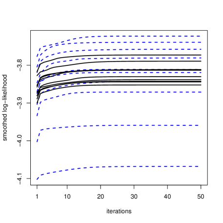
Figure 1: Values of the empirical smoothed log-likelihood at each step of the algorithm, for the first ten replications. Black plain lines: $n=900$. Blue dotted lines: $n=300$.

Figure 2 shows the sum of the estimated squared biases and variances for the copula parameter vector. The variance is $3$ times higher than the squared bias for $n=300$, and only $1.6$ times higher for $n=900$. While the bias remains stable, the variance decreases with $n$, but at a slower rate than the “parametric” rate $1/n$. While $n=900$ is $3$ times larger than $n=300$, the variance at $n=900$ is only $1.5$ times smaller than the variance at $n=300$. The mean absolute bias is about $\sqrt{0.5/3}\approx 0.4$, while the mean standard errors at $n=300$ and $n=900$ are about $\sqrt{1.2/3}\approx 0.63$ and $\sqrt{0.8/3}\approx 0.52$, respectively.

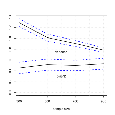
Figure 2: Estimated squared bias and variance of the copula parameter vector estimator for various sample sizes at the last step of the algorithm. Dashed blue lines represent 95% confidence bands (aka simultaneous confidence intervals) obtained from an application of the multivariate central limit theorem to the five hundred replications.

Figure 3 shows the marginal density estimates at the last step of the algorithm for $n=900$, for the last replication. The estimates agree well with the true marginal densities. We noticed, however, that they were similar to the initial estimates.

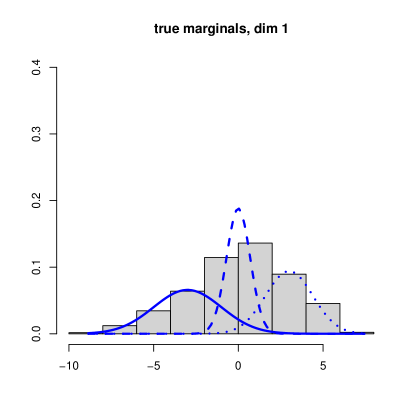
(a)

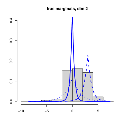
(b)

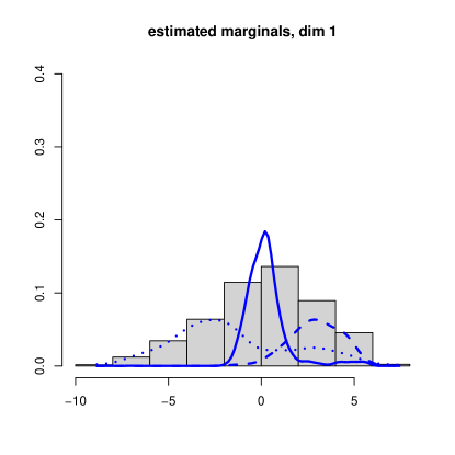
(c)

(d)

Figure 3: True and estimated marginal densities of the three clusters and the two dimensions for $n=900$ (last replication). The top row contains the true marginals and the column on the left contains the first dimension. The marginal estimates are those found at the last step of the algorithm.

5 Conclusion

An algorithm was designed and implemented to estimate the parameters of copula-based semiparametric mixture models. The model considered is a very general one since it does not assume any specific structure (such as the location-scale assumption) on marginal densities. The algorithm is deterministic, and hence always returns the same result if fed with the same initial point. Good performance was obtained in an illustrative numerical example, which suggests that the algorithm may indeed be monotonic under appropriate conditions.

However, its theoretical analysis proved to be challenging and only partial results were obtained for versions of the algorithm where either the copula parameter or the marginals were fixed. A future avenue of research may consist of rejecting those updates where the smoothed log-likelihood does not increase and investigate whether convergence results of Meyer (1976); Zangwill (1969) could be applied. To simplify, the full parametric case may first be considered. To improve the numerical implementation of the algorithm, the integral (3) may be computed with other methods, such as Qiang (2010). The sensitivity of the algorithm with respect to initialization may be investigated further, however.

References

• Allman et al. (2009) Allman, E. S., Matias, C., and Rhodes, J. A. (2009). Identifiability of parameters in latent structure models with many observed variables. The Annals of Statistics, 37(6A):3099–3132.
• Benaglia et al. (2009) Benaglia, T., Chauveau, D., and Hunter, D. R. (2009). An EM-like algorithm for semi-and nonparametric estimation in multivariate mixtures. Journal of Computational and Graphical Statistics, 18(2):505–526.
• Bonhomme et al. (2016) Bonhomme, S., Jochmans, K., and Robin, J.-M. (2016). Non-parametric estimation of finite mixtures from repeated measurements. Journal of the Royal Statistical Society: Series B (Statistical Methodology), 78(1):211–229.
• Brezis (2011) Brezis, H. (2011). Functional analysis, Sobolev spaces and partial differential equations. Springer.
• Kasahara and Shimotsu (2014) Kasahara, H. and Shimotsu, K. (2014). Non-parametric identification and estimation of the number of components in multivariate mixtures. Journal of the Royal Statistical Society: Series B (Statistical Methodology), 76(1):97–111.
• Kwon and Mbakop (2021) Kwon, C. and Mbakop, E. (2021). Estimation of the number of components of nonparametric multivariate finite mixture models. The Annals of Statistics, 49(4):2178–2205.
• Levine et al. (2011) Levine, M., Hunter, D. R., and Chauveau, D. (2011). Maximum smoothed likelihood for multivariate mixtures. Biometrika, 98(2):403–416.
• Mazo (2017) Mazo, G. (2017). A semiparametric and location-shift copula-based mixture model. Journal of Classification, 34(3):444–464.
• Mazo and Averyanov (2019) Mazo, G. and Averyanov, Y. (2019). Constraining kernel estimators in semiparametric copula mixture models. Computational Statistics & Data Analysis, 138:170–189.
• Meyer (1976) Meyer, R. R. (1976). Sufficient conditions for the convergence of monotonic mathematical programming algorithms. Journal of Computer and System Sciences, 12:108–121.
• Nelsen (2007) Nelsen, R. B. (2007). An introduction to copulas. Springer Science & Business Media.
• Qiang (2010) Qiang, J. (2010). A high-order fast method for computing convolution integral with smooth kernel. Computer Physics Communications, 181(2):313–316.
• Rau et al. (2015) Rau, A., Maugis-Rabusseau, C., Martin-Magniette, M.-L., and Celeux, G. (2015). Co-expression analysis of high-throughput transcriptome sequencing data with Poisson mixture models. Bioinformatics, 31(9):1420–1427.
• Wu and Lange (2010) Wu, T. T. and Lange, K. (2010). The MM alternative to EM. Statistical Science, 25(4):492–505.
• Xiang et al. (2019) Xiang, S., Yao, W., and Yang, G. (2019). An Overview of Semiparametric Extensions of Finite Mixture Models. Statistical Science, 34(3):391–404. Publisher: Institute of Mathematical Statistics.
• Zangwill (1969) Zangwill, W. I. (1969). Nonlinear Programming—A Unified Approach. Prentice-Hall.