Sequential decompositions at their limit
Abstract
Sequential updating (SU) decompositions are a well-known technique for creating profit and loss (P&L) attributions, e.g., for a bond portfolio, by dividing the time horizon into subintervals and sequentially editing each risk factor in each subinterval, e.g., FX, IR or CS. We show that SU decompositions converge for increasing number of subintervals if the P&L attribution can be expressed by a smooth function of the risk factors. We further consider average SU decompositions, which are invariant with respect to the order or labeling of the risk factors. The averaging is numerically expensive, and we discuss several ways in which the computational complexity of average SU decompositions can be significantly reduced.
Keywords profit and loss attribution; sequential decompositions; change analysis; risk decomposition
Mathematics Subject Classification (2020) 60H05, 60H30, 91G05, 91G10, 91G60, 91G30, 91G40
JEL Classification C02, C30, C63, D31, D33
1 Introduction
Profit and loss (P&L) attribution has a long history in risk management. P&L attribution is the process of analyzing change between two valuation dates and explaining the development of the P&L by the movement of the sources (risk factors) between the two dates, see Candland and Lotz (2014). In other words, the change in the P&L over time is decomposed with respect to the different risk factors to explain how each factor contributes to the P&L.
There are numerous desirable properties that a decomposition should have, see Shorrocks (2013) and Fortin (2011). It should be symmetric, i.e., the contributions of the risk factors should be independent of the way in which the factors are labeled or ordered. Symmetric decompositions are sometimes also called path-independent, see Biewen (2012) and Fortin (2011). A decomposition should also be exact or additive, which means that the sum of all contributions is equal to the total change in the P&L.
A common method for creating decompositions is to sequentially update the risk factors one by one while “freezing” all other risk factors. This idea dates back at least to 1973, see Oaxaca (1973) and Blinder (1973), who developed a sequential updating (SU) decomposition technique in a static setting to decompose the wage gap between people from different groups. Candland and Lotz (2014) refer to the static SU decomposition as a waterfall and applied it for P&L attribution. DiNardo et al. (1996) use a sequential updating method to analyze recent changes in wage distribution in the United States. See Fortin (2011) for an overview on how the SU decomposition principle is used in various fields of economics. The SU decomposition is additive by construction, but it depends on the order in which the risk factors are updated. That is, if there are risk factors, there are different update orders and therefore possible ways to compute the SU decomposition.
A popular alternative to the sequential updating concept is the so-called one-at-a-time (OAT) decomposition, see Biewen (2012), Candland and Lotz (2014) and Jetses and Christiansen (2022), which is closely related to SU decompositions. The OAT decomposition is called bump and reset in Candland and Lotz (2014). The OAT decomposition is symmetric, but in general not additive, since the joint variations of the risk factors are not taken into account.
With the aim of carrying out surplus decompositions in life insurance, Jetses and Christiansen (2022) and Christiansen (2022) extended Biewen (2012) to multiperiod settings by dividing the time horizon into subintervals and recursively applying the SU method on each subinterval. Similarly, Frei (2020) proposed a multiperiod setting based on the OAT method. Multiperiod SU and OAT decompositions depend on the time grid, and there are infinite possibilities to choose that time grid. In practice, one typically works with yearly, quarterly, monthly or daily steps. To eliminate the dependence on the grid, Jetses and Christiansen (2022) and Christiansen (2022) investigated the limits of SU and OAT decompositions when the length of the subintervals approaches zero, and they arrived at infinitesimal sequential updating (ISU) decompositions and infinitesimal one-at-a-time (IOAT) decompositions. Jetses and Christiansen (2022) showed in an insurance context that the ISU decomposition is not only additive but also symmetric if there are no interaction effects in the sense that the covariations between the risk factors are zero. Christiansen (2022) proved that the ISU decomposition is symmetric if it is stable with respect to small perturbations in the empirical observation of the risk factors. In Appendix A.4, we show that the ISU decomposition of a simple product of two correlated Brownian motions is not stable. This shows that stability is a rather strong assumption.
With the aim of defining an additive decomposition principle that is invariant with respect to the order or labeling of the risk factors, Shorrocks (2013) and Jetses and Christiansen (2022) introduced the ASU and IASU decompositions, respectively, which are simply the arithmetic average of the possible SU/ISU decompositions. The (static) ASU decomposition is also called Shapley decomposition, see Shorrocks (2013). The ASU and IASU decompositions are additive and symmetric by construction. Compared to multiperiod ASU decompositions, IASU decompositions have the advantages that they do not depend on the choice of a time grid and that they take the whole trajectories of the risk factors into account. In a model setting without interaction effects or jumps, Mai (2023) proposes a decomposition that is equivalent to the IASU decomposition, splitting the P&L of a portfolio into four parts: P&L due to changes in foreign exchange rate, interest rate, calendar time and market risk.
Table 1 provides an overview of the various decomposition principles SU/ISU, OAT/ IOAT and ASU/ IASU, with focus on the properties of additivity, symmetry and computational complexity. The table summarizes that the limit-based decompositions generally have more favorable properties, so investigating the limits is not just a theoretical exercise but of practical value. In particular, the IASU decomposition is computationally preferable to the ASU decomposition if there are no simultaneous jumps in the risk factors.
| Contribution of | No int. effects | No simul. jumps | General case | |||||||
|---|---|---|---|---|---|---|---|---|---|---|
| SU | vary while is consecutively fixed | a | c | a | c | a | c | |||
| ISU | limes of SU | a | s | c | a | c | a | c | ||
| OAT | vary while is fixed at origin | s | c | s | c | s | c | |||
| IOAT | limes of OAT | a | s | c | s | c | s | c | ||
| ASU | average of SU | a | s | a | s | a | s | |||
| IASU | average of ISU | a | s | c | a | s | c | a | s | |
In game theory, the Shapley decomposition is better known as Shapley value. Young (1985) shows that the Shapley value satisfies certain desirable properties. The Shapley decomposition has been introduced axiomatically to risk allocation, see for example Denault (2001) and Powers (2007). The Shapley decomposition is also relevant in the context of portfolio optimization, see Shalit (2020), income inequality analysis, see Shorrocks (2013) and Sastre and Trannoy (2002), and carbon emission reduction, see Yu et al. (2014) and Albrecht et al. (2002). An axiomatic introduction to P&L attribution, which leads to the Shapley decomposition, can be found in Moehle et al. (2021, Sec. 3.1), where efficient calculations and numerical approximations of the Shapley decomposition are also discussed, e.g., reducing the numerical complexity from to .
There are various other decomposition principles as well: Fischer (2004) uses a conditional expectations approach. Gatzert and Wesker (2014) analyze the impact of different types of mortality risk on the risk situation in life insurance. Norberg (1999) and Ramlau-Hansen (1991) discuss surplus decomposition in life insurance within a Markov framework. Rosen and Saunders (2010) use the Hoeffding method for a decomposition of credit risk portfolios. Frei (2020) uses the Euler principle for risk attribution. Schilling et al. (2020) investigate the case of a one period model and provide a list of six desirable properties of decomposition methods. These authors use a method based on the martingale representation theorem, which satisfies all of their six properties, but which is only applicable to processes that are martingales.
In many applications, the P&L or price of an asset can be expressed as a smooth function of the underlying (risk) factors. For example, the price of a foreign stock is simply the product of the foreign exchange rate and the stock price in its domestic currency. The price of a zero-coupon foreign corporate bond can be expressed by
where is the foreign exchange rate, is the interest rate, is the credit spread, is the calendar time and is the maturity of the bond. In this article, we aim to decompose with respect to , where is a -dimensional semimartingale describing the evolution of risk factors and is a twice continuously differentiable function.
This paper makes the following contributions. In Sect. 3, we provide a rigorous definition of SU decomposition for arbitrary update orders in the risk factors. In Sect. 4, we prove that the ISU decomposition of twice continuously differentiable functions of the risk factors always exists, and we provide an explicit formula. In Sect. 5 we analyze the IOAT and IASU decompositions and compare the three different decomposition methods. In Sect. 6 we provide sufficient conditions under which the computational complexity for calculating the IASU decomposition can be significantly reduced. In Sect. 7 we discuss several examples of P&L attributions and study an example on the decomposition of a value-at-risk process. Sect. 8 concludes the manuscript.
2 Notation
We use a similar setting as in Schilling et al. (2020) and Christiansen (2022). Let be a filtered probability space satisfying the usual conditions. Let be a -dimensional semimartingale, and let be the natural filtration of . The process is called a risk basis or information basis, and its components are denoted as risk factors or sources of risk. Let be the set of all -semimartingales. Let be the set of twice differentiable functions from to . For and , we write and for the partial derivatives and . Let be a map. For example, can be defined by , for some . The aim of this paper is to decompose with respect to . For two semimartingales and and a càglàd process , we denote by the stochastic integral. In particular by convention. We further set ,
Let denote the minimum of real numbers and , respectively. For a stopping time and a vector of stopping times , we define stopped semimartingales as follows:
We denote the -row of a real matrix by
For a sequence of stopping times and , we denote by the vector of stopping times
We define for and as follows:
In other words, is the left limit of at time at the positions where is equal to zero.
3 SU decomposition principle
Similar to Shorrocks (2013) and Christiansen (2022), we call a -dimensional process the decomposition of . A decomposition is called additive or exact if
We interpret as the contribution of to for . A decomposition principle does not need to be additive, see for example the one-at-time decomposition in Biewen (2012) and Jetses and Christiansen (2022), which has remaining interaction effects. However, additivity is certainly a desirable property in many applications, see Shorrocks (2013) and Christiansen (2022).
Example 3.1.
Assume , for some . Itô’s formula states that
| (3.1) |
for
| (3.2) |
if the risk basis has continuous paths and the covariations between different risk factors are zero, i.e. for . Hence, is an additive decomposition.
If the risk factor stays constant on , it does not contribute to and the contribution of should be zero. This is reflected precisely by the normalization axiom in Christiansen (2022). Therefore, it seems naturally to define the contribution of for Example 3.1 as in Eq. (3.2). If there are interaction effects or discontinuous paths, the sequential updating (SU) decomposition is still able to define a reasonable decomposition along an unbounded partition of , i.e.
and we will see in Theorem 4.2 that the SU decomposition converges to a process that generalizes the decomposition in Example 3.1 if the step sizes of the partition approach zero.
Before formally defining the SU decomposition, we provide a motivation based on telescoping series for the case . That is, we decompose with respect to and for some . The difference could be the P&L of some asset depending on the risk factors in the time interval . For instance, the price of a foreign stock in domestic currency could be expressed by , where is the exchange rate and is the price of the stock in the foreign currency. Then, by using a telescoping series,
| (3.3) |
Here, the interval is divided into smaller subintervals , and in each subinterval risk factor is updated first, while the other risk factor stays constant. Then is updated while is fixed. We write Eq. (3.3) in shorter notation. Let , . Then,
| (3.4) |
The first sum on the right-hand side of Eq. (3.4) is the sum of all the differences from the right-hand side of Eq. (3.3), where varies, and we interpret it as the contribution of to . The second sum of Eq. (3.4) is interpreted as the contribution of .
One could also go the other way around and update first in each subinterval and then . So, in case of , there are two possible SU decompositions, which are formally defined below in Definition 3.3.
We generalize the example above slightly by allowing the unbounded partition to depend on . We recall the following definition from Protter (1990, p. 64).
Definition 3.2.
An infinite sequence of finite stopping times such that a.s. is called unbounded random partition. A sequence of unbounded random partitions is said to tend to the identity if a.s. for .
Definition 3.3 (SU decomposition, case ).
Let be an unbounded random partition. The SU (sequential updating) method with respect to defines two decompositions and of for by
and
For , the processes and both describe the contribution of to . Next, we define the SU decomposition principle for arbitrary dimensions. The notation is inspired by Biewen (2012, Sec. 3.3). Let . Matrix is defined by
Let , where is the set of all permutations of . Matrix is defined by
Matrix permutes the columns and rows of by . Let
where is the identity matrix. Then, and are identical except at the main diagonal, where has a chain of ones and has a chain of zeros.
Example 3.4.
For and with , , ,
Definition 3.5 (SU decomposition, ).
Let be an unbounded random partition. The SU (sequential updating) method with respect to defines a set of decompositions of by
| (3.5) |
where and .
Definition 3.5 generalizes Definition 3.3. If , then and the SU decomposition reduces to the formula stated in Jetses and Christiansen (2022) and Christiansen (2022). We extend their proof that the SU decomposition is additive for arbitrary order of the risk basis and for random partitions. Note that the Assumption (3.6) in the next proposition is satisfied if for some it holds that .
Proposition 3.6.
Assume for any finite stopping time that
| (3.6) |
The sum in Eq. (3.5) is almost surely a finite sum and the SU decomposition is almost surely additive.
4 ISU decomposition principle
Jetses and Christiansen (2022) and Christiansen (2022) investigated the limits of SU decompositions for time-grids with vanishing step sizes, this way introducing ISU decompositions. While Jetses and Christiansen (2022) define ISU decompositions pointwise for each time point, it is more convenient to follow the definition of Christiansen (2022), who uses (deterministic) partitions that apply for the whole timeline. We generalize Christiansen (2022) and define the ISU decomposition with respect to random partitions. In Theorem 4.2, we give some sufficient conditions that ensure the existence of ISU decompositions.
Definition 4.1.
Let be a sequence of unbounded random partitions tending to the identity. For , let be the SU decomposition of with respect to and . If the limits
exist in probability, then is called the ISU (infinitesimal sequential updating) decomposition of with respect to order and partition sequence .
Theorem 4.2.
Let . Then, the ISU decomposition of exists for each order and each sequence of unbounded random partitions tending to the identity. For and , it almost surely equals
| (4.1) |
Remark 4.3.
If is of finite variation, one can unify the part in the last line of Eq. (4.2) with the first integral,
where
How does the SU decomposition treat simultaneous jumps in the limit? and are identical except for the -position, where and . Hence, the term
describes the change of if we allow to go from to and fix all other , at some limiting time-point depending on . The next example sheds some more light on the contribution of the jumps for the ISU decomposition for the case .
Example 4.4.
Assume is a pure-jump semimartingale of finite variation. Then Itô’s formula states that
| (4.2) |
Here, in contrast to Example 3.1, Itô’s formula does not provide much insight on how to decompose the right-hand-side of Eq. (4.2) with respect to . Assume and . Then based on telescoping series,
The case can be discussed similarly, using
Remark 4.5.
As shown in Example 3.1, it is straightforward to define a reasonable contribution of using Itô’s formula and the normalization axiom from Christiansen (2022) if has continuous paths and there are no interaction effects. Eq. (4.2) contains Example 3.1 as a special case. If there are interaction effects, then Eq. (4.2) assigns the interaction effects and possible jumps in a way that depends on the order of the risk factors. The IASU decomposition solves this issue by taking the average over all possible permutations , see Sec. 5. The concrete interpretation of the individual terms in Eq. (4.2) depends on the application, several examples are discussed in Sec. 7.
The next example shows that the smoothness assumptions for in Theorem 4.2 are important for the existence of the ISU decomposition.
Example 4.6.
Let be a stochastic process with independent increments and . Jumps of shall only occur at fixed times and for each , the process jumps by with equal probability for upward and downward movements. The process stays constant between jumps. Then, is a semimartingale, see Černỳ and Ruf (2021). Let
so . Let be a deterministic sequence of unbounded partitions tending to the identity such that set contains the first smallest elements of , but its intersection with is empty. Assume that . Then, for it follows that
| (4.3) |
which is divergent for , so the ISU decomposition does not exist here.
If the risk factors have no simultaneous jumps, then Eq. (4.2) can be significantly simplified.
Corollary 4.7.
Let . If have no simultaneous jumps, the ISU decomposition of with respect to is almost surely given for and for by
| (4.4) |
Proof.
Remark 4.8.
Suppose that the covariations between different risk factors are zero, i.e. for . In particular, this implies , i.e. the risk factors have no simulatenous jumps. In this case, the ISU decomposition becomes invariant with respect to , i.e., the ISU decomposition does not depend on the order or labeling of the risk factors. This has also been observed by Jetses and Christiansen (2022) in an insurance context.
5 One-at-a-time and average decompositions
Another common decomposition principle originates from the OAT (one-at-a-time) method, which is discussed in Jetses and Christiansen (2022), Biewen (2012) and Candland and Lotz (2014). In contrast to SU decompositions, OAT decompositions are symmetric but not additive. In Corollary 5.2, we will show that OAT decompositions also exists in the limit. However, interaction effects between the risk factors are not assigned to any particular risk factor, see Corollary 5.6 below.
Definition 5.1 (OAT decomposition).
Let be an unbounded random partition. The OAT (one-at-a-time) decomposition with respect to defines a decomposition of for and for by
If the limit of OAT decompositions exists in probability for an increasing sequence of unbounded random partitions tending to the identity, then this limit is called IOAT (infinitesimal one-at-a-time) decomposition.
Theorem 5.2.
Let . Then, the IOAT decomposition of exists for each sequence of unbounded random partitions. For and , it almost surely equals
| (5.1) |
Proof.
If the covariations between the risk factors are not simply zero, then additive and symmetric decompositions can be obtained by averaging the possible SU/ISU decompositions, see Shorrocks (2013) and Jetses and Christiansen (2022).
Definition 5.3.
Let and be the SU and ISU decompositions, respectively, with respect to . For and for , the ASU and IASU decompositions are defined by
As the next corollary shows, if the risk factors have no simultaneous jumps, then the computationally expensive averaging vanishes in the IASU decomposition.
Corollary 5.4.
Let . If have no simultaneous jumps, the IASU decomposition of is almost surely given for and for by
| (5.2) |
Proof.
Example 5.5.
How does the IASU decomposition treat simultaneous jumps? Let and assume that is a pure-jump semimartingale of finite variation. Then the IASU decomposition is equal to
compare with Example 4.4. The latter formulas are averages of sequential updates from time point to time point .
The three decomposition principles ISU, IOAT and IASU have a particularly appealing form if is continuous, as the next corollary shows.
Corollary 5.6.
Let have almost surely continuous paths, and define
The ISU decomposition for a permutation of is given for and for by
| (5.4) |
The IOAT decomposition of is given for and for by
| (5.5) |
The IASU decomposition of is given for and for by
| (5.6) |
Proof.
Remark 5.7.
In Corollary 5.6, the three decompositions differ only in the attribution of the interaction effects . For the ISU decomposition, the interaction effects are assigned to the different risk factors depending on the order of the risk basis. In the case of the IOAT decomposition, interaction effects are not assigned to any particular risk factor but have to be reported separately. The IOAT decomposition is therefore not additive. The IASU decomposition, on the other hand, assigns half of the interaction effect to each risk factor and , i.e., it splits the interaction effects “fifty-fifty”. If the components of have simultaneous jumps, Theorem 4.2 and Corollary 5.2 show that the ISU principle treats simultaneous jumps depending on , the IOAT principle ignores simultaneous jumps and the IASU principle takes the average over simultaneous jumps, compare with Example 5.5.
Remark 5.8.
In case that the risk factors have continuous paths and no interaction effects, the ISU, IOAT and IASU decompositions are equal. In this case the OAT decomposition is asymptotically additive, as already proven in Frei (2020).
6 Numerical approximation of the IASU decomposition
How can the IASU decomposition be efficiently calculated in practice? If we naively approximate the integrals in Eq. (5.2) numerically, then we may loose perfect additivity of the decomposition, which is undesirable in many applications. As an alternative, one could approximate the IASU decomposition by ASU decompositions with vanishing step sizes in the time-grid, which is justified by Theorem 4.2. The latter approximation approach perfectly maintains additivity, but the computational complexity advantage of the IASU decomposition according to Corollary 5.4 is lost. The next corollary offers a way that maintains both, perfect additivity and the computational complexity advantage in case that the risk factors have no simultaneous jumps.
Corollary 6.1.
Let . Assume that have no simultaneous jumps. The IASU decomposition of can then be obtained from the average of two ISU decompositions, i.e.,
where is the identity, i.e., , and is the ”reverse“ identity, i.e., for .
In practice, Corollary 6.1 can be applied as follows: approximate the two ISU decompositions by two SU decompositions with vanishing step sizes in the time-grid, which is justified by Theorem 4.2. This computationally cheap approach produces perfectly additive numerical approximations of the IASU decomposition.
In the next corollary, we show that computational complexity can be further reduced if has an advantageous structure, e.g., if can be described as a sum of smooth functions that do not each depend on all of the risk factors. This may, for instance, be the case with a (large) portfolio where each individual asset depends only on a few risk factors. For example, a foreign investment in stocks has risk factors: the stocks and the foreign exchange rates. The next corollary shows that in this example, we need only instead of SU decompositions to approximate the IASU decomposition.
Corollary 6.2.
Let , and assume that
for functions that depend only on risk factors for . The IASU decomposition of can then be obtained from ISU decompositions.
Proof.
By Theorem 4.2, the IASU decomposition is linear in the argument . The assertion follows then immediately because the IASU decomposition of can be obtained by ISU decompositions. ∎
Example 6.3.
Annually, the EIOPA (European Insurance and Occupational Pensions Authority) performs a market and credit risk comparison study. All participating insurance companies have to model the risk of different synthetic instruments, which are used to build a set of realistic investment portfolios. The benchmark portfolios consist of about instruments in total, which cover all relevant asset classes, i.e., risk-free interest rates, sovereign bonds, corporate bonds, equity indices and property, see Table A2 in Flaig and Junike (2022) for an overview. Approximately risk factors are necessary to evaluate all instruments. Each individual instrument has up to three risk factors (exposure to foreign currencies is supposed to be hedged). For example, a France sovereign bond with five years left to maturity is an instrument that has three risk factors: EUR interest rate (5y), France credit spread (5y) and time decay. A linear combination of all instruments builds a portfolio with price , where , is a (weighted) instrument and depends on three or fewer risk factors. Corollary 6.2 implies that no more than SU decompositions need to be computed to obtain the ASU decomposition of that portfolio. A naive approach to obtain the ASU decomposition would require SU decompositions.
7 Applications
In this section, we provide some applications. In Sect. 7.1, we consider a European investor who invests in the US stock market, and we decompose her P&L and her one-year value at risk. In Sect. 7.2, we provide a formula for the P&L attribution of a call option on some stock, and in Section 7.3 we decompose the P&L of a foreign corporate zero-coupon bond into the follwing four contributions: foreign exchange rate, interest rate, credit spread and calendar time.
7.1 P&L and VaR decomposition of a foreign stock in domestic currency
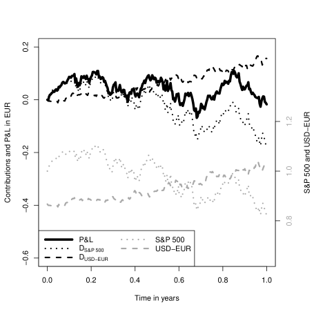
Consider an European investor investing in the US market, i.e. the domestic currency is EUR and the foreign currency is USD. Let be the price in USD of an exchange traded fund (ETF) replicating the S&P 500 index and let describe the USD-EUR exchange rate (price of 1 USD in EUR). The product describes the price of the ETF measured in EUR. The return is driven by the S&P 500 and USD-EUR exchange rate in a product structure. What is the contribution of the stock movements to the overall P&L, and what is the contribution of the evolution of the currency rate to the overall P&L?
We decompose the price of a foreign stock, where is the foreign exchange rate and is the stock price in the foreign currency. As observed by Mai (2023), the instantaneous P&L of the foreign stock in home currency is given by
i.e., it can be decomposed into the variation in the foreign exchange rate, variation in the stock price and interaction effects. The latter is distributed equally between and , as the next corollary shows.
Corollary 7.1.
Let and . Then, for , the IASU decomposition is equal to
Figure 1 shows the P&L in EUR of an investment in the S&P 500 over the time horizon of one year. It can be seen that the exchange rate has risen by , while the S&P 500 has fallen by over the time horizon. This has the effect that both risk factors cancel each other out at , such that the P&L in EUR barely changes over the time horizon of one year. Accordingly, the contributions of the S&P 500 and the exchange rate are of similar size but have opposite sign.
Next, we look at the value at risk over some time interval of the product of two geometric Brownian motions describing, for instance, the value of a foreign stock in domestic currency. We first formally define the value at risk . The following definition is in the spirit of Example 11.7 in Föllmer and Schied (2016). denotes the space of finite valued random variables. By , we denote the smallest -Algebra that contains all , .
Definition 7.2.
Let . Let be a Algebra. Let be a measurable random variable. The conditional value at risk of given at level is defined by
The essential infimum is defined in Föllmer and Schied (2016, Thm A.37) and recalled in Sect. A.3. Given , the probability that is greater than is less than or equal to a.s. Let denote the cumulative distribution function of a lognormal distribution with parameters and , i.e., the distribution function of the random variable , where is standard normal.
Proposition 7.3.
Let and be correlated geometric Brownian motions, i.e.,
for two independent Brownian motions , and , and . Let
For a fixed time horizon and , it holds that
Proof.
Let . Let
where is a standard normal random variable independent of . For the conditional value at risk,
∎
Hence, the conditional value at risk is equal to the product of and weighted by . For the IASU decomposition of the conditional value at risk,
we obtain
The processes and capture the changes in the conditional value at risk of due to movements in and , respectively.
7.2 P&L decomposition of a call option
Assume a Black–Scholes market with a stock and a call option on the stock. So the stock price process
is a geometric Brownian motion for some . The price of a call option with strike , maturity and interest rate can be described by
where is the calendar time, and
Here, is the cumulative distribution function of the standard normal distribution, and
Now, the P&L of a call option in the Black–Scholes model is decomposed with respect to stock price movement and calendar time, i.e. the information basis is the two-dimensional process . For , the IASU decomposition yields
where , and are the Delta, Gamma and Theta of the call option. As shown in Eq. (2) in Carr and Wu (2020), we can attribute the instantaneous P&L of the option investment to the variation in calendar time and stock price by
i.e., captures price movements and second-order effects and captures calendar time.
7.3 P&L decomposition of a foreign zero-coupon bond
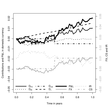
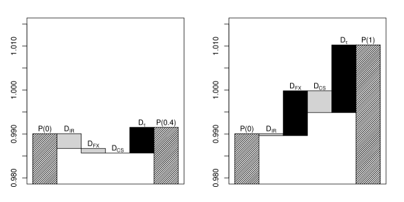
Assume that the price of a foreign, zero-coupon bond with maturity can be described by , where
is the (continuous compounded) interest rate (IR), is the credit spread (CS), and is some foreign exchange rate (FX), possibly correlated with and . The IASU decomposition with respect to risk factors , , and calendar time yields
where
are the interaction effects between the interest rate and foreign exchange rate. That is, captures foreign exchange rate movements, captures interest rate movements, represents credit spread evolution and captures calendar time effects. , , and also include second-order and interaction effects.
Let us model the interest rate by a Vasicek model, which can be described by the following stochastic differential equation, see Brigo and Mercurio (2001, Sec. 3.2):
where , , , and is a Brownian motion. Foreign exchange rate is modeled by a geometric Brownian motion:
where and is a Brownian motion correlated with by . Process is modeled by a pure jump process, which starts at zero and jumps from to at time , independent of and . For the maturity of the bond, we choose .
8 Conclusion
It is common practice to use sequential updating (SU) decompositions on finite time-grids to obtain profit and loss attributions of portfolios. In this article, we provided a formal definition of SU decompositions for multiple time periods and arbitrary orders of the risk factors. We analyzed the case in which the P&L of the portfolio can be described by a twice differentiable function of the risk factors. We allowed for nontrivial interaction effects and describe the risk factors by semimartingales. We proved the existence of ISU decompositions as stochastic limits of SU decompositions with vanishing step sizes in the time-grids. To obtain a symmetric decomposition, i.e., a decomposition that does not depend on the order or labeling of the risk factors, we studied averages over all permutations of ISU decompositions, giving a closed form that has a computational complexity . For cases where the risk factors have no simultaneous jumps, we provided a simplification that reduces computational complexity to . We also discussed several examples and showed that in many applications the P&L can indeed be described by a twice differentiable function of the risk factors.
Acknowledgements
We thank Bernd Buchwald and Andreas Märkert from Hannover Re, Solveig Flaig from Deutsche Rück and Jan-Frederik Mai from XAIA investment for very fruitful discussions that helped to improve this paper.
Appendix A Appendix
A.1 Proof of Theorem 4.2
Proof.
We use standard arguments from the proof of Itô’s formula, see for example Protter (1990, Thm. 32, Part II), but many new arguments are also needed. Let . Fix some and some permutation . For , let be a sequence of unbounded random partitions tending to the identity. To keep the notation simple, we use the following abbreviations: for a matrix , let
and denote the matrices containing only zeros and only ones, respectively. Instead of and , we simply write and , respectively. By using Protter (1990, Thm. 21 and 30, Part II), for , it holds that
| (A.1) |
| (A.2) |
where denotes convergence in probability. We use the fact that a sequence of random variables converges in probability if and only if every subsequence has a further subsequence that converges almost surely. Let be a subsequence of the sequence . There is another subsequence of such that the sums in Eqs. (A.1–A.2) almost surely converge. Let be the maximal subset such that for all , the paths are càdlàg functions, Eq. (A.15) holds, the sums in Eqs. (A.1–A.2) surely converge on along subsequence , and surely on for all and for . Then, . We will show that the SU decomposition with respect to converges for all surely as . This implies that the SU decomposition converges in probability.
In the next steps of the proof, we assume that is fixed. Let be the closure of set . The path is càdlàg and takes a maximum value on the compact set . This implies that is bounded and hence compact. The convex hull of the compact set is also compact by Carathéodory’s theorem, see Grünbaum (2013, Sec. 2.3). Considering the definition of and ,
| (A.3) |
which implies that and and hence that and that
| (A.4) |
Let , and let be defined as in Lemma A.2, i.e., contains all time points in , where at least one component of has jumps that are greater than . SU decomposition with respect to can be written as
| (A.5) |
where and
We now analyze the first sum on the right-hand side of Eq. (A.5). The first sum of Eq. (A.5) converges as to
| (A.6) |
We will later need the following observation: let us develop around using Taylor expansion and Eq. (A.3), to obtain
where is the remainder of the Taylor expansion; see Lemma A.3. The term has a similar representation replacing by and by . Hence, for some that only involves quadratic terms ,
| (A.7) |
We now analyze the second sum of the right-hand side of Eq. (A.5). We develop around by using a Taylor expansion, see Lemma A.3 and by using Eq. (A.4). It holds that
| (A.8) |
The last equation follows by looking at the four cases: 1) , 2) , 3) and , and 4) and . The remainder is defined by
and for some ,
is similarly defined. Using and Eq. (A.8), the second sum of the right-hand side of Eq. (A.5) can be written as
| (A.9) |
The first, second and third sums of the right-hand side of Eq. (A.9) converge by the definition of sequence for to some stochastic integrals. The fourth sum of Eq. (A.9) converges for to
| (A.10) |
Adding the sums in Eqs. (A.10) and (A.6), we obtain
| (A.11) | |||
| (A.12) | |||
| (A.13) |
Note that and all its derivatives take a maximum on the set , which is compact. By using Eq. (A.7), each of the three sums only depend on quadratic terms and by Lemma A.1, the sums (A.11), (A.12) and (A.13) are absolutely convergent for and converge for to
Finally, we treat the remainder. Applying the same arguments as those in the proof of the classical Itô’s formula can show that the remainder converges to zero; note that and the second derivatives of are uniformly continuous on . Hence, for any , there is a such that for all ,
where denotes the Euclidean norm. This implies that there is a nondecreasing function such that for and
where we applied Eq. (A.16) as well. Let . Let such that
| (A.14) |
which exists according to Lemma A.2. Eq. (A.14) implies that the largest absolute jump of for is less than . Note that . Therefore,
i.e. the remainder is arbitrarily small for to be close enough to zero. ∎
A.2 Auxiliary results
Lemma A.1.
Let be a -dimensional semimartingale. Then, for all ,
| (A.15) |
Proof.
For any numbers , ; hence,
| (A.16) |
This implies that
∎
Lemma A.2.
Let such that the path is càdlàg, and Eq. (A.15) holds. Let and
contains all time points in , where at least one component of has jumps greater than . Then, contains a finite number of points. Let
Then, the sequence converges. Furthermore, for any , there is a such that
Proof.
Lemma A.3 (Taylor’s theorem).
Let open. Let such that for all Let be twice continuously differentiable. Then,
where the remainder can be expressed for some and by
Proof.
Forster (2017, Satz 2, Sec. 7). ∎
A.3 Essential infimum
The following theorem and definition are taken from Föllmer and Schied (2016).
Theorem A.4.
Let be a set of random variables. There exists a random variable such that
- i
-
a.s. for all
- ii
-
for all such that a.s. for all .
Proof.
Föllmer and Schied (2016, Thm. A.37). ∎
Definition A.5.
in the Theorem is called the essential supremum of . In Notation
The essential infimum is defined by
A.4 Stability
In this section, we use the notation in Christiansen (2022). For , let with for all . The function
is called a delay. A delay is called phased if there is an unbounded partition of such that on each interval , at most one component of is nonconstant. Let be a refining sequence of delays that increase to identity (rsdii), i.e.,
Let be a set containing at least one phased rsdii. Let be a semimartingale, and define
Let
Let be the set of càdlàg processes starting in zero and let . A map is called decomposition scheme of . assigns each a decomposition of . The ISU decomposition scheme is abbreviated . A decomposition scheme is called stable at if
for all rsdii .
Proposition A.6.
Assume that with for a Brownian motion . Let be a simple product. Then, there is a set of continuous phased rsdii such that the ISU decomposition of is not stable at .
Proof.
Suppose that contains a continuous phased rsdii with . For a partition of such that is constant on , let . In addition, let also contain .
Since and by the multidimensional Taylor theorem,
By the definitions of , and ,
for . Let denote the Stratonovich integral and denote the Itô integral. Let and plim denote the convergence in probability; then,
With the same arguments,
for . Therefore,
for , and hence, the ISU decomposition of cannot be stable at . ∎
References
- Albrecht et al. (2002) Albrecht, J., François, D., Schoors, K.: A Shapley decomposition of carbon emissions without residuals. Energy policy 30(9), 727–736 (2002)
- Biewen (2012) Biewen, M.: Additive decompositions with interaction effects. IZA Discussion Paper (2012)
- Blinder (1973) Blinder, A.S.: Wage discrimination: reduced form and structural estimates. J. Hum. Resour. 436–455 (1973)
- Brigo and Mercurio (2001) Brigo, D., Mercurio, F.: Interest rate models: theory and practice, vol. 2. Springer, New York (2001)
- Candland and Lotz (2014) Candland, A., Lotz, C.: Profit and Loss attribution. In: Internal Models and Solvency II – From Regulation to Implementation, Risk Books, London (2014)
- Carr and Wu (2020) Carr, P., Wu, L.: Option profit and loss attribution and pricing: a new framework. J. Finance 75(4), 2271–2316 (2020)
- Černỳ and Ruf (2021) Černỳ, A., Ruf, J.: Pure-jump semimartingales. Bernoulli 27(4), 2624–2648 (2021)
- Christiansen (2022) Christiansen, M.C.: On the decomposition of an insurer’s profits and losses. Scand. Actuar. J. 1–20 (2022)
- Denault (2001) Denault, M.: Coherent allocation of risk capital. J. Risk 4, 1–34 (2001)
- DiNardo et al. (1996) DiNardo, J., Fortin, N., Lemieux, T.: Labor market institutions and the distribution of wages, 1973-1992: A semiparametric approach. Econometrica 64(5), 1001–1044 (1996)
- Fischer (2004) Fischer, T.: On the decomposition of risk in life insurance. Working Paper, Technische Universität Darmstadt (2014)
- Flaig and Junike (2022) Flaig, S., Junike, G.: Scenario generation for market risk models using generative neural networks. Risks 10(11), 199 (2022)
- Föllmer and Schied (2016) Föllmer, H., Schied, A.: Stochastic Finance. de Gruyter, Berlin (2016)
- Forster (2017) Forster, O.: Analysis 2: Differentialrechnung im , gewöhnliche Differentialgleichungen. Springer-Verlag, New York (2017)
- Fortin (2011) Fortin, N., Lemieux, T., Firpo, S.: Decomposition methods in economics. In Volume 4, Part A of Handbook of Labor Economics. Elsevier 10, P. Amsterdam: S0169-7218. (2011)
- Frei (2020) Frei, C.: A new approach to risk attribution and its application in credit risk analysis. Risks 8(2), 65 (2020)
- Gatzert and Wesker (2014) Gatzert, N., Wesker, H.: Mortality risk and its effect on shortfall and risk management in life insurance. J. Risk Insur. 81(1), 57–90 (2014)
- Grünbaum (2013) Grünbaum, B.: Convex polytopes. In: Graduate Texts in Mathematics, vol. 221. Springer, New York (2013)
- Jetses and Christiansen (2022) Jetses, J., Christiansen, M.C.: A general surplus decomposition principle in life insurance. Scand. Actuar. J. 1–25 (2022)
- Mai (2023) Mai, J.F.: Performance attribution w.r.t. rates, FX, carry, and residual market risks. arXiv preprint arXiv:2302.01010 (2023).
- Moehle et al. (2021) Moehle, N., Boyd, S., Ang, A.: Portfolio performance attribution via Shapley value. arXiv preprint arXiv:2102.05799 (2021)
- Norberg (1999) Norberg, R.: A theory of bonus in life insurance. Finance Stoch. 3(4), 373–390 (1999)
- Oaxaca (1973) Oaxaca, R.: Male-female wage differentials in urban labor markets. Int. Econ. Rev. 693–709 (1973)
- Powers (2007) Powers, M.R.: Using Aumann-Shapley values to allocate insurance risk: the case of inhomogeneous losses. N. Am. Actuar. J. 11(3), 113–127 (2007)
- Protter (1990) Protter, P.: Stochastic differential equations. In: Stochastic Integration and Differential Equations. Springer, New York (1990)
- Ramlau-Hansen (1991) Ramlau-Hansen, H.: Distribution of surplus in life insurance. ASTIN Bull. 21(1), 57–71 (1991)
- Rosen and Saunders (2010) Rosen, D., Saunders, D.: Risk factor contributions in portfolio credit risk models. J. Bank. Financ. 34(2), 336–349 (2010)
- Sastre and Trannoy (2002) Sastre, M., Trannoy, A.: Shapley inequality decomposition by factor components: Some methodological issues. J. Econ. 9(1), 51–89 (2002)
- Schilling et al. (2020) Schilling, K., Bauer, D., Christiansen, M.C., Kling, A.: Decomposing dynamic risks into risk components. Manag. Sci. 66(12), 5738–5756 (2020)
- Shalit (2020) Shalit, H.: The Shapley value of regression portfolios. J. Asset Manag. 21(6), 506–512 (2020)
- Shorrocks (2013) Shorrocks, A.F.: Decomposition procedures for distributional analysis: a unified framework based on the Shapley value. J. Econ. Inequal. 11(1), 99–126 (2013)
- Young (1985) Young, H.P.: Monotonic solutions of cooperative games. Int. J. Game Theory 14(2), 65–72 (1985)
- Yu et al. (2014) Yu, S., Wei, Y., Wang, K.: Provincial allocation of carbon emission reduction targets in China: An approach based on improved fuzzy cluster and Shapley value decomposition. Energy policy 66, 630–644 (2014)