Transfer Learning with Large-Scale Quantile Regression

Abstract

Quantile regression is increasingly encountered in modern big data applications due to its robustness and flexibility. We consider the scenario of learning the conditional quantiles of a specific target population when the available data may go beyond the target and be supplemented from other sources that possibly share similarities with the target. A crucial question is how to properly distinguish and utilize useful information from other sources to improve the quantile estimation and inference at the target. We develop transfer learning methods for high-dimensional quantile regression by detecting informative sources whose models are similar to the target and utilizing them to improve the target model. We show that under reasonable conditions, the detection of the informative sources based on sample splitting is consistent. Compared to the naive estimator with only the target data, the transfer learning estimator achieves a much lower error rate as a function of the sample sizes, the signal-to-noise ratios, and the similarity measures among the target and the source models. Extensive simulation studies demonstrate the superiority of our proposed approach. We apply our methods to tackle the problem of detecting hard-landing risk for flight safety and show the benefits and insights gained from transfer learning of three different types of airplanes: Boeing 737, Airbus A320, and Airbus A380.

Keywords: data fusion; hard landing; informative source; robust regression; targeted learning

1 Introduction

Quantile regression (Koenker and Bassett Jr, 1978; Koenker and Hallock, 2001) is commonly encountered in modern applications. It goes beyond mean regression and allows the relationship between the outcome of interest and the features to vary across the conditional quantiles of the outcome distribution. One prominent example arises in analyzing and predicting hard landing for flights with Quick Access Recorder (QAR) data (Wang et al., 2014; Chen and Jin, 2021), where the main objective is to study the risk of high vertical acceleration at the touchdown point of a flight with measurements from QAR during the flight. There are thousands of QAR measurements, while the number of flights is relatively small for some airplane models, such as the Airbus-380. Such high-dimensional but small-sample quantile regression problems (Belloni and Chernozhukov, 2011; Wang et al., 2012) are prevalent in a variety of fields. Some other examples include the modeling of the quantiles of suicide risk (Rogers and Joiner, 2018) to identify high-risk patients with medical diagnoses and medication records from electronic health records (EHR), and the use of quantile regression to reveal a comprehensive picture of the varying effects of market factors on asset pricing (Maiti, 2021). Applications with quantile regression are also seen in actuarial science (Baione and Biancalana, 2021), finance (Demir et al., 2022), environmental research (Reich, 2012), and medical studies (Wei et al., 2006; Huang et al., 2017). For an overview of the theory, methods and applications of quantile regression, we refer to Koenker et al. (2017).

In many applications, the goal is to learn the conditional quantiles of an outcome for a specific target population, while the available data may go well beyond the target and may be from various other sources that bear certain similarities with the target. For example, in the airplane hard landing problem, an investigator may be only interested in Airbus-380, for which the target population consists of only flights with Airbus-380; however, data from other airplanes such as Airbus-320 or Boeing-737 may also be available. In healthcare, a specific healthcare provider, e.g., a children’s medical center, may only be interested in building a risk prediction model of a disease/condition for its own patient population, while patient data from other age ranges or other hospitals may also be available (Xu et al., 2022). In asset pricing, the main interest may be on a new portfolio with limited historical data, while much more data may be available on other similar portfolios or market indices like S&P 500 index (Gu et al., 2020).

In all the above problems, a crucial question is how to properly transfer the information from the sources to the target to best perform the estimation and inference of the conditional quantiles for the target. Apparently, neither the approach of only using the information pertaining to the target or the approach of naively combining all the available information to fit a one-size-fits-all model would work well. While the former fails to seek any potential gain by completely ignoring the additional information from the sources, the latter may result in “negative transfer” (Rosenstein et al., 2005) by ignoring the potential heterogeneity among the sources and the target. Such heterogeneity may arise from various aspects and ultimately makes the transfer learning problem challenging. First, even if we assume the sources and the target share the same set of features, these features may follow different distributions across the sources and the target. Second, the true model of the target may not be the same as that of each of the sources; rather, it is more realistic to assume that these models can be different and only a subset of source models may be similar enough to the target model to permit “positive transfer”. Last but not the least, the error distributions of different models could be different, not only in their magnitudes (variances) and types (Gaussian vs. non-Gaussian), but also in their quantile levels. To our knowledge, existing transfer learning frameworks mainly deal with the first and the second types of heterogeneity. Bastani (2021) designed a two-step procedure (proxy step and joint step) of transfer learning for high-dimensional linear regression with one target and one source. Li et al. (2021) proposed a procedure to realize transfer learning of high-dimensional linear models between one target and several sources, which first trains a fusion model with all data and then performs debiasing with the target data. Tian and Feng (2023) made an extension along the same line for the generalized linear models. A concurrent study from Huang et al. (2023) explored the direct extension of the two-step framework proposed in Li et al. (2021) for quantile regression models. See Pan and Yang (2009), Weiss et al. (2016), and Cheng et al. (2020) for some comprehensive surveys on transfer learning in machine learning, statistics, and engineering.

We propose a novel transfer learning procedure for high-dimensional quantile regression to properly utilize information from external data sources while allowing for all three types of heterogeneity in feature distributions, model coefficients, and error distributions. Our approach is built upon the two-step framework in Li et al. (2021), and a transformation step is added to handle the heterogeneity of the error types and quantile levels, which is specific to quantile regression problems (Chen et al., 2020). Compared with Li et al. (2021) and Tian and Feng (2023), our proposed method relaxes the condition on error distribution and enables transfer learning for quantile regression with a non-differentiable loss. Comparing with Huang et al. (2023), our proposed method executes sparse quantile regression problems distributively on the different sources rather than pooling them and utilizes surrogate responses to avoid the quantile loss, making our method more suitable for large-scale real-world applications. We develop an informative-source detection procedure based on sample splitting and show that under reasonable conditions, the procedure is consistent. Compared to the naive model fitted with the target data alone, the proposed transfer-learning model enjoys a sharper convergence rate as a function of sample sizes, signal-to-noise ratio, and similarities among the target and the source models. Extensive simulation studies verify the superiority of our approach. We apply the proposed approach to tackle the problem of detecting hard-landing risk for flight safety, and show that with the help of Airbus-320 and Boeing-737 datasets, the transfer learning model for Airbus-380 gives more accurate estimation and the resulting feature contributions are visualized and highly interpretable.

The rest of the paper is organized as follows. In Section 2, we present the transfer learning setup with high-dimensional quantile regression. We propose the estimation procedures via transfer learning in Section 3 and provide their theoretical guarantees in Section 4. Numerical experiments and the application on airplane hard-landing are provided in Section 5 and Section 6, respectively. Section 7 gives some concluding remarks and future research directions. All the technical details are provided in the Appendix.

2 Transfer Learning Setup for Quantile Regression

Before carrying out the model setup, we introduce some notations. For two constants $c_{1}$ and $c_{2}$, we denote $c_{1}\vee c_{2}=\max(c_{1},c_{2})$ and $c_{1}\wedge c_{2}=\min(c_{1},c_{2})$. For a vector $\boldsymbol{v}={({{v_{1}},\ldots,{v_{n}}})^{\top}}$, we denote $\|\boldsymbol{v}\|_{0}=\sum\nolimits_{i=1}^{n}I(v_{i}\neq 0)$ where $I(\cdot)$ is the indicator function as the $\ell_{0}$ norm, $\|\boldsymbol{v}\|_{1}=\sum\nolimits_{i=1}^{n}|{{v_{i}}}|$ as the $\ell_{1}$ norm, $\|\boldsymbol{v}\|=\sqrt{\sum\nolimits_{i=1}^{n}{v_{i}^{2}}}$ as the $\ell_{2}$ norm, and $\|\boldsymbol{v}\|_{\infty}={\max_{i}}|{{v_{i}}}|$ as the infinity norm of $\boldsymbol{v}$. For a matrix $\boldsymbol{A}\in{R^{n\times n}}$, we denote its infinity norm ${\|\boldsymbol{A}\|_{\infty}}={\max_{i}}\sum\nolimits_{j=1}^{n}{|{{A_{ij}}}|}$. For two sequences $\{{{a_{n}}}\}_{n=1}^{\infty}$ and $\{{{b_{n}}}\}_{n=1}^{\infty}$, we denote ${a_{n}}\asymp{b_{n}}$ if and only if ${a_{n}}=O({{b_{n}}})$ and ${b_{n}}=O({{a_{n}}})$. For two non-zero real sequences $\{{{c_{n}}}\}_{n=1}^{\infty}$ and $\{{{d_{n}}}\}_{n=1}^{\infty}$, ${c_{n}}\gg{d_{n}}$ stands for $|{{c_{n}}/{d_{n}}}|\to 0$. We use $\lesssim$ and $\gtrsim$ to indicate that the inequality holds up to some multiplicative numerical constant.

Our main interest is to learn the conditional quantiles of an outcome variable of interest, $y^{(0)}\in\mathbb{R}$, given a set of feature variables, $\boldsymbol{x}^{(0)}\in\mathbb{R}^{p}$, at a specified target population. We assume that the following quantile regression model holds at the target,

$$\left\{\begin{array}[]{l}y^{(0)}=\boldsymbol{x}^{(0)^{\top}}{\boldsymbol{\beta}_{\tau}^{\left(0\right)}}+\epsilon^{(0)};\\ {\mathbb{P}}\left({\epsilon^{(0)}\leq 0}\right)={\tau},\end{array}\right.$$ (1)

where ${\boldsymbol{\beta}_{\tau}^{(0)}}$ is the true regression coefficient for the target population under the quantile level $\tau$, and $\epsilon^{(0)}\in{\mathbb{R}}$ is the random error term with a density function ${f^{(0)}}(\cdot)$. When $\tau$ is specified and no confusion arises, we may abbreviate ${\boldsymbol{\beta}_{\tau}^{(0)}}$ as $\boldsymbol{\beta}^{(0)}$. To deal with high dimensionality, we assume that the true coefficient vector $\boldsymbol{\beta}^{(0)}$ is sparse with $s_{0}$ nonzero elements and ${\|{{\boldsymbol{\beta}^{(0)}}}\|_{\infty}}$ is bounded. Here $\boldsymbol{x}^{(0)}$ is independent of the noise $\epsilon^{(0)}$, and that the density of $\epsilon^{(0)}$ exists with ${\mathbb{P}}({\epsilon^{(0)}\leq 0})=\tau$. This model thus allows the error term to be heavy-tailed, such as Cauchy distribution or $t$ distribution. It is worth noting that the true coefficient vector $\boldsymbol{\beta}^{(0)}$ is the solution of the following population-level optimization problem

$$\boldsymbol{\beta}^{(0)}=\mathop{\rm arg\,min}_{\boldsymbol{\beta}\in{{\mathbb{R}}^{p}}}{\mathbb{E}}\rho_{\tau}\left(y^{(0)}-\boldsymbol{x}^{(0)^{\top}}\boldsymbol{\beta}\right),$$ (2)

where $\rho_{\tau}(u)=u(\tau-I(u\leq 0))$ is the quantile loss function (Koenker, 2005).

In addition to the target population, suppose we also have access to $K$ source populations with the same set of features and the same response. For each $k=1,\ldots,K$, we assume that the following source-specific quantile regression model holds,

$$\left\{\begin{array}[]{l}y^{(k)}={\boldsymbol{x}^{(k)^{\top}}}{\boldsymbol{\beta}_{\tau}^{\left(k\right)}}+\epsilon^{(k)};\\ {\mathbb{P}}\left({\epsilon^{(k)}\leq 0}\right)={\tau}.\end{array}\right.$$ (3)

Here the regression coefficient vector ${\boldsymbol{\beta}_{\tau}^{(k)}}$ or simply ${{\boldsymbol{\beta}^{(k)}}}$, can be different from that of the target $\boldsymbol{\beta}^{(0)}$. Similarly, we assume $\boldsymbol{\beta}^{(k)}$ has bounded infinity norm, sparse with $s_{k}$ nonzero elements, and the error term $\epsilon^{(k)}$ is independent with ${{\boldsymbol{x}^{(k)}}}$ and satisfies the same density quantile condition. ${f^{(k)}}(\cdot)$ is the density function of the random error $\epsilon^{(k)}$.

Intuitively, the rationale of transfer learning is that, if some of the source models are similar “enough” to the target model, we may expect these sources to provide additional valuable information about the target model. It is then pivotal to quantify the similarity between the target model in (1) and the source models in (3). A natural idea is to use the $\ell_{1}$ distance between the coefficient vector of the target model and that of each source model, i.e., $\|{\boldsymbol{\delta}^{(k)}}\|_{1}=\|\boldsymbol{\beta}^{(0)}-\boldsymbol{\beta}^{(k)}\|_{1}$. When this distance is smaller than certain threshold $d>0$, we say that the $k$th source is $d$-informative. Consequently, we define

$$\mathcal{A}=\left\{{1\leq k\leq K:{\|\boldsymbol{\delta}^{\left(k\right)}}\|_{1}\leq d}\right\}$$

to be the $d$-informative set.

Now suppose we observe $n_{0}$ independently and identically distributed (i.i.d.) samples from the target population under the model in (1), consisting of a feature matrix $\boldsymbol{X}^{(0)}=(\boldsymbol{x}_{1}^{(0)},\ldots,\boldsymbol{x}_{n_{0}}^{(0)})^{\top}\in{\mathbb{R}}^{n_{0}\times p}$ whose rows are i.i.d. from Gaussian distribution with mean zero and covariance matrix ${\boldsymbol{\Sigma}^{(0)}}$, and a response/outcome vector $\boldsymbol{y}^{(0)}=(y_{1}^{(0)},\ldots,y_{n_{0}}^{(0)})^{\top}\in{\mathbb{R}}^{n_{0}}$. In addition to the target data, suppose we also have i.i.d. samples from each of the $K$ source populations under the models in (3). For $k=1,\ldots,K$, the data from source $k$ are denoted as $\{(\boldsymbol{X}^{(k)},\boldsymbol{y}^{(k)})\}_{k=1}^{K}$ with $\boldsymbol{X}^{(k)}\in{\mathbb{R}}^{n_{k}\times p}$ whose rows are i.i.d. from Gaussian distribution with mean zero and covariance matrix ${\boldsymbol{\Sigma}^{(k)}}$, and $\boldsymbol{y}^{(k)}\in{\mathbb{R}}^{n_{k}}$ where $n_{k}$ is the sample size at source $k$. In the sequel we denote ${\underline{n}}=\min_{k=1}^{K}{n_{k}}$, ${\underline{n}_{{\cal A}}}={\min_{k\in{{\cal A}\cup\{0\}}}}{n_{k}}$, and ${\overline{n}_{{\cal A}}}={\max_{k\in{{\cal A}\cup\{0\}}}}{n_{k}}$.

Our main task is then to develop a transfer learning procedure to estimate $\boldsymbol{\beta}^{(0)}$ in the target model (1) with both the target data $(\boldsymbol{X}^{(0)},\boldsymbol{y}^{(0)})$ and the additional source data $\{(\boldsymbol{X}^{(k)},\boldsymbol{y}^{(k)})\}_{k=1}^{K}$. In particular, we are interested in clarifying how the potential benefit of transfer learning is related to the specifications of the error distributions, the distributional-shift of the features, the dimensions and sparsity levels of the models, and the similarity levels of the sources models to the target.

Before we dive into the transfer learning approach, we first present a model that one would use if only provided the target data. Specifically, we consider the following $\ell_{1}$-penalized quantile regression estimator

$$\widehat{\boldsymbol{\beta}}{}^{(0)}=\mathop{\rm arg\,min}_{\boldsymbol{\beta}\in{{\mathbb{R}}^{p}}}\frac{1}{n_{0}}\sum_{i=1}^{n_{0}}\rho_{\tau}(y_{i}^{(0)}-{\boldsymbol{x}_{i}^{(0)^{\top}}}\boldsymbol{\beta})+\lambda_{0}\left\|\boldsymbol{\beta}\right\|_{1},$$ (4)

where $\lambda_{0}$ is the regularization parameter. This estimator enjoys consistency and support recovery properties under some regular conditions on the target data (Fan et al., 2014). We refer to this method as the “target-only method” which serves as the baseline to be compared with transfer-learning approach.

3 Estimation Procedures via Transfer Learning

We develop procedures for estimating the quantile regression model at the target via transfer learning. We start with the oracle case that the informative set $\mathcal{A}$ is given and then consider the estimation of the informative set $\mathcal{A}$ to complete the puzzle.

3.1 Oracle Procedure with Known Informative Set

Suppose the informative set ${\cal A}$ is given, that is, we’ve known a priori that it is the most beneficial to consider information transfer from the sources belonging to ${\cal A}$. In this case, we realize transfer learning by a four-step procedure, consisting of (1) single-source modeling, (2) response surrogation, (3) fusion learning, and (4) debiasing.

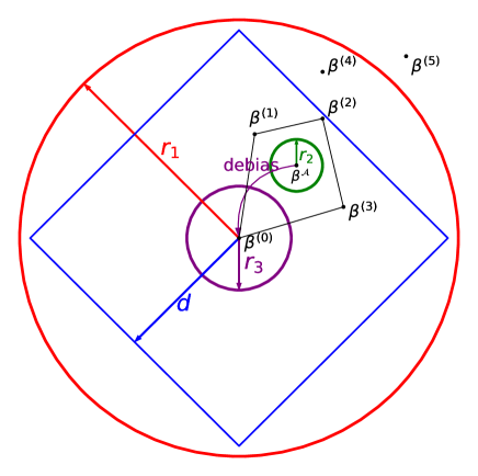
Figure 1: Schematic of the procedures in transfer learning quantile regression.

Figure 1, inspired by Figure 5 in Tian and Feng (2023), illustrates how the proposed procedure can possibly lead to an improved estimator of $\boldsymbol{\beta}^{(0)}$ with information from the informative sources. With the limited sample size $n_{0}$ at the target, the convergence rate of the target-only estimator under $\ell_{2}$-norm is ${r_{1}}=\sqrt{{s_{0}}{\log({p\vee{n_{0}}})}/{n_{0}}}$, which is the radius of the red circle centered at the true coefficient vector $\boldsymbol{\beta}^{(0)}$. Suppose sources 1, 2, and 3 are $d$-informative among the five sources, their corresponding true coefficient vectors ${\boldsymbol{\beta}^{(1)}}$, ${\boldsymbol{\beta}^{(2)}}$, and ${\boldsymbol{\beta}^{(3)}}$ are then within the blue square. To start the algorithm, firstly, for each $k\in{\cal A}\cup\{0\}$, we estimate $\boldsymbol{\beta}^{(k)}$ using $\ell_{1}$-penalized quantile regression as in (4) (Step 1), and then adopt the method in Chen et al. (2020) to construct surrogate responses in order to simplify the quantile regression problem to linear regression (Step 2). Steps 1 and 2 are designed to locate ${\boldsymbol{\beta}^{(1)}}$, ${\boldsymbol{\beta}^{(2)}}$ and ${\boldsymbol{\beta}^{(3)}}$ as the best linear regression coefficients of the surrogate responses on their covariates. The third and the fourth steps then conduct fusion learning and debiasing, respectively (Li et al., 2021). To be more specific, Step 3 locates $\widehat{\boldsymbol{\beta}}{}^{\cal A}$ through combining information from the target and the informative sources; this is with a convergence rate $r_{2}$ (the radius of the green circle) and the estimator is inside the convex hull established by ${\boldsymbol{\beta}^{(k)}}$, $k\in{\cal A}\cup\{0\}$. The exact location of ${\boldsymbol{\beta}^{\mathcal{A}}}$, which is the target or the probabilistic limit for $\widehat{\boldsymbol{\beta}}{}^{\cal A}$, is determined by a weighted linear transformation of the $\boldsymbol{\beta}^{(k)}$s from the informative sources, where the weights are associated with the sample size and the feature covariance matrix of each source. More details can be found in Section A in the Appendix. Finally, Step 4 performs debiasing only using the target information, by which the final estimator is within the circle around $\boldsymbol{\beta}^{(0)}$ with a radius $r_{3}$. Typically, $r_{3}$ is expected to be larger than $r_{2}$ due to a bias-variance trade-off, but it could be much smaller than $r_{1}$, the convergence rate of the target-only model.

The details of our proposed procedure are presented below.
Step 1 (Single-source modeling): For each $k\in{\cal A}\cup\{0\}$, we estimate $\widehat{\boldsymbol{\beta}}{}^{(k)}$ by an $\ell_{1}$-penalized quantile regression,

$$\widehat{\boldsymbol{\beta}}{}^{(k)}=\mathop{\rm arg\,min}_{\boldsymbol{\beta}\in{{\mathbb{R}}^{p}}}{\frac{1}{{{n_{k}}}}\sum\limits_{i=1}^{{n_{k}}}\{\tau-I({y_{i}^{\left(k\right)}-\boldsymbol{x}_{i}^{(k)^{\top}}\boldsymbol{\beta}\leq 0})\}\left({y_{i}^{\left(k\right)}-\boldsymbol{x}_{i}^{(k)^{\top}}\boldsymbol{\beta}}\right)}+{\lambda_{0}}\left\|\boldsymbol{\beta}\right\|_{1}.$$ (5)

Step 2 (Response surrogation): For each $k\in{\cal A}\cup\{0\}$, the kernel density estimator for the density of the error evaluated at the point of zero is given by

$${{\widehat{f}}^{\left(k\right)}}(0)=\frac{1}{{n_{k}}h^{\left(k\right)}}\sum\limits_{i=1}^{{n_{k}}}G\left(\frac{y_{i}^{\left(k\right)}-\boldsymbol{x}_{i}^{(k)^{\top}}{\widehat{\boldsymbol{\beta}}{}^{\left(k\right)}}}{h^{\left(k\right)}}\right),$$ (6)

where $G$ is a kernel function satisfying Assumption 6 (to be shown in Section 4) with $h^{(k)}$ being its bandwidth. A surrogate response is then constructed as

$$\widetilde{y}_{i}^{\left(k\right)}=\boldsymbol{x}_{i}^{{{\left(k\right)}^{\top}}}{\widehat{\boldsymbol{\beta}}{}^{\left(k\right)}}-\{{\widehat{f}}^{\left(k\right)}(0)\}^{-1}\left\{{I\left({y_{i}^{\left(k\right)}-\boldsymbol{x}_{i}^{(k)^{\top}}{\widehat{\boldsymbol{\beta}}{}^{\left(k\right)}}\leq 0}\right)-\tau}\right\},\qquad i=1,\ldots,n_{k}.$$ (7)

Denote ${{\widetilde{\boldsymbol{y}}}^{(k)}}=(\widetilde{y}_{1}^{(k)},\ldots,\widetilde{y}_{n_{k}}^{(k)})^{\top}$ as the surrogate response vector.

Step 3 (Fusion learning): We fit an $\ell_{1}$-penalized regression with the surrogate responses ${\widetilde{\boldsymbol{y}}}^{(k)}$ with all data

$$\widehat{\boldsymbol{\beta}}{}^{\cal A}=\mathop{\rm arg\,min}_{\boldsymbol{\beta}\in{{\mathbb{R}}^{p}}}\frac{1}{2(n_{\cal A}+{n_{0}})}\sum_{k\in{\cal A}\cup\{0\}}\left\|{\widetilde{\boldsymbol{y}}}^{(k)}-\boldsymbol{X}^{(k)}\boldsymbol{\beta}\right\|^{2}+{\lambda_{1}}\left\|\boldsymbol{\beta}\right\|_{1},$$ (8)

where $n_{\cal A}=\sum_{k\in\cal A}n_{k}$ is the total sample size of $\cal A$.

Step 4 (Debiasing): We fit an $\ell_{1}$-penalized regression with the target data

$${\widehat{\boldsymbol{\delta}}{}^{\cal A}}=\mathop{\arg\min}\limits_{\boldsymbol{\delta}\in{{\mathbb{R}}^{p}}}\frac{1}{{2{n_{0}}}}{\left\|{{{\widetilde{\boldsymbol{y}}}^{\left(0\right)}}-{\boldsymbol{X}^{\left(0\right)}}\left({{\widehat{\boldsymbol{\beta}}{}^{\cal A}}-\boldsymbol{\delta}}\right)}\right\|^{2}}+{\lambda_{2}}{\left\|\boldsymbol{\delta}\right\|_{1}}$$ (9)

Finally, the oracle quantile regression estimator is given as

$${\widehat{\boldsymbol{\beta}}}={\widehat{\boldsymbol{\beta}}{}^{\mathcal{A}}}-{\widehat{\boldsymbol{\delta}}{}^{\mathcal{A}}}.$$ (10)

In comparison to the concurrent study by Huang et al. (2023), our proposed estimation method could lead to superior computational efficiency in large-scale settings. The fusion learning step in the concurrent study solves a pooled $\ell_{1}$-penalized quantile regression with sample size $n_{\cal A}$. In contrast, our method trains a $\ell_{1}$-penalized quantile regression for the target and each source individually, which can be implemented in parallel with computation time now largely driven by the maximum local sample size ${{\max}_{k\in{\cal A}\cup\{0\}}}n_{k}$. Moreover, our subsequent fusion step with the pooled samples becomes a Lasso problem through the adoption of the surrogate response, which is much easier to solve than its counterpart of $\ell_{1}$-penalized quantile regression.

3.2 Identification of Informative Set

In the previous section, the informative set ${\cal A}$ is assumed to be known as a priori, which is not practical in many real applications. Motivated by Tian and Feng (2023), we develop an effective method to detect the informative set ${\cal A}$.

The proposed detection method has three steps. Firstly, we randomly split the target data into two sub-samples of equal size, one for training (${\cal I}$) and another for testing (${\cal I}^{c}$). Second, we run the transfer learning procedure with each source data and the target training data, to produce a set of single-source transfer learning estimators. These transfer learning estimators are evaluated on the target testing data. Finally, we determine the informative sources by comparing the losses incurred by the transfer learning estimators to that of the target-only estimator. Figure 2 illustrates the procedure of informative sources detection and shows its similarity to the idea of cross validation. The blue lines indicate the operations related to the half of the target data for training (blue half-circle on the right), and the red lines indicate the operations related to the other half of the target data for testing (red half-circle on the left), while the black lines indicate the comparisons between the target-only estimator and the single-source transfer learning estimators for the detection of informative sources.

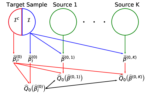
Figure 2: Schematic of the procedures in informative set detection.

To present the details, we first introduce the loss function that is used to evaluate the estimators. The population-level loss on the target model is defined as

$${Q_{0}}\left(\boldsymbol{\beta}\right)={\mathbb{E}}\left\{{{{\left({\widetilde{y}^{(0)}-{\boldsymbol{x}^{(0)^{\top}}}\boldsymbol{\beta}}\right)}^{2}}}\right\},$$ (11)

where $\widetilde{y}^{(0)}={\boldsymbol{x}^{(0)^{\top}}}{\boldsymbol{\beta}^{(0)}}-\{{f^{(0)}}(0)\}^{-1}\{{I({y^{(0)}-{\boldsymbol{x}^{(0)^{\top}}}{\boldsymbol{\beta}^{(0)}}\leq 0})-\tau}\}$ and the expectation is taken with respect to the target distribution. This loss function was adopted by Chen et al. (2020) in a distributed quantile regression setting. The corresponding finite-sample loss evaluated on the target testing samples, with indices $i\in{\cal I}^{c}$, is calculated as:

$${\widehat{Q}_{0}}\left(\boldsymbol{\beta}\right)=\frac{1}{{{n_{0}/2}}}\sum\limits_{i\in{{\cal I}^{c}}}{{{\left({\widetilde{y}_{i}^{(0)}-\boldsymbol{x}_{i}^{(0)^{\top}}\boldsymbol{\beta}}\right)}^{2}}},$$ (12)

where $\widetilde{y}_{i}^{(0)}=\boldsymbol{x}_{i}^{(0)^{\top}}\widehat{\boldsymbol{\beta}}{}_{{{\cal I}^{c}}}^{(0)}-\{{{\widehat{f}}^{(0)}}(0)\}^{-1}\{{I({y_{i}^{(0)}-\boldsymbol{x}_{i}^{(0)^{\top}}\widehat{\boldsymbol{\beta}}{}_{{{\cal I}^{c}}}^{(0)}\leq 0})-\tau}\}$ and

$${{\widehat{f}}^{\left(0\right)}}(0)=\frac{2}{{n_{0}}h_{{\cal I}^{c}}^{\left(0\right)}}\sum\limits_{i\in{{\cal I}^{c}}}{G\left({\frac{{y_{i}^{(0)}-\boldsymbol{x}_{i}^{(0)^{\top}}\widehat{\boldsymbol{\beta}}{}_{{{\cal I}^{c}}}^{\left(0\right)}}}{h_{{\cal I}^{c}}^{\left(0\right)}}}\right)},$$

with $\widehat{\boldsymbol{\beta}}{}_{{{\cal I}^{c}}}^{(0)}$ denoting the $\ell_{1}$-penalized quantile regression estimator with the target testing data.

With the above definitions, the detailed procedure for detecting the informative set ${\cal A}$ is as follows.

Step 1: We randomly divide the target sample into two subsamples $S_{1}=(\boldsymbol{X}^{(0)}_{\cal I},\boldsymbol{y}^{(0)}_{\cal I})$, $S_{2}=(\boldsymbol{X}^{(0)}_{{\cal I}^{c}},\boldsymbol{y}^{(0)}_{{\cal I}^{c}})$, where ${\cal I}$ is a subset of $\{1,2,\ldots,n_{0}\}$ with cardinality $|{\cal I}|\approx n_{0}/2$. Then we calculate $\widehat{\boldsymbol{\beta}}{}_{\cal I}^{(0)}$ by performing $\ell_{1}$-penalized quantile regression with $S_{1}$. For each $1\leq k\leq K$, we obtain $\widehat{\boldsymbol{\beta}}{}^{(0,k)}$ by running Steps 1–3 in Section 3.1 with the sample $({\boldsymbol{X}_{\cal I}^{(0)},\boldsymbol{y}_{\cal I}^{(0)}})\cup({{\boldsymbol{X}^{(k)}},{\boldsymbol{y}^{(k)}}})$.

Step 2: On $S_{2}=(\boldsymbol{X}^{(0)}_{{\cal I}^{c}},\boldsymbol{y}^{(0)}_{{\cal I}^{c}})$, we run $\ell_{1}$-penalized quantile regression to obtain $\widehat{\boldsymbol{\beta}}{}_{{{\cal I}^{c}}}^{(0)}$, then calculate the loss $\widehat{Q}_{0}(\widehat{\boldsymbol{\beta}}{}_{\cal I}^{(0)})$ and $\widehat{Q}_{0}(\widehat{\boldsymbol{\beta}}{}^{(0,k)})$ defined in (12) for each $k\in\{1,2,\ldots,K\}$.

Step 3: The estimated informative set is

$$\widehat{\cal A}=\left\{{1\leq k\leq K:{{\widehat{Q}}_{0}}\left({{\widehat{\boldsymbol{\beta}}{}^{\left(0,k\right)}}}\right)\leq\left({1+{\varepsilon_{0}}}\right){{\widehat{Q}}_{0}}\left(\widehat{\boldsymbol{\beta}}{}_{\cal I}^{\left(0\right)}\right)}\right\},$$ (13)

with a given small value $\varepsilon_{0}\in({0,c_{\varepsilon}}]$ that controls the strictness of selection. Here $c_{\varepsilon}$ is a constant that satisfies Assumption 8 below. In practice, we can estimate ${c_{\varepsilon}}$ as,

$${\widehat{c}_{\varepsilon}}=\mathop{\inf}\limits_{k\in\left\{{1,\ldots,K}\right\}}\frac{{{{\left({{{\widehat{\boldsymbol{\beta}}{}}^{\left(k\right)}}-{{\widehat{\boldsymbol{\beta}}{}}^{\left(0\right)}}}\right)}^{\top}}{{\widehat{\boldsymbol{\Sigma}}{}}^{\left(0\right)}}\left({{{\widehat{\boldsymbol{\beta}}{}}^{\left(k\right)}}-{{\widehat{\boldsymbol{\beta}}{}}^{\left(0\right)}}}\right)}}{{{{\widehat{Q}}_{0}}\left({{{\widehat{\boldsymbol{\beta}}{}}^{\left(0\right)}}}\right)}}$$ (14)

where ${\widehat{\boldsymbol{\beta}}{}^{(k)}}$, $k=0,\ldots,K$ are the initial single-source estimators from (5), and $\widehat{\boldsymbol{\Sigma}}{}^{(0)}$ is an empirical estimator of ${\boldsymbol{\Sigma}^{(0)}}$ with the target data, e.g., the sample covariance matrix of $\boldsymbol{X}^{(0)}$.

Finally, we run the proposed transfer learning procedure in Section 3.1 with $\widehat{\cal A}$ to obtain our Trans-Lasso quantile regression estimator, denoted as $\widetilde{\boldsymbol{\beta}}$, to be distinguished from the oracle estimator $\widehat{\boldsymbol{\beta}}{}$ defined in (10).

4 Theoretical Analysis

We impose the following assumptions.

Assumption 1 (Sparsity).

For each $k=0,1,\ldots,K$, let ${S_{k}}=\{{0\leq i\leq p:\beta_{i}^{(k)}\neq 0}\}$ and ${s_{k}}=|S_{k}|$, and assume ${s_{k}}=O({n_{k}^{r}})$ for some $0<r<1/3$.

Assumption 2 (Feature distributions).

For each $k=0,1,\ldots,K$, the rows of $\boldsymbol{X}^{(k)}$ are i.i.d. Gaussian distributed with mean zero and covariance matrix ${{\boldsymbol{\Sigma}}^{(k)}}$. The eigenvalues of each ${{\boldsymbol{\Sigma}}^{(k)}}$ are bounded away from 0 and $\infty$.

With the potential distributional-shift in features, i.e., ${{\boldsymbol{\Sigma}}^{(k)}}$s are allowed to be different, the following measurments are defined to quantify the maximum difference between ${{\boldsymbol{\Sigma}}^{(0)}}$ and ${{\boldsymbol{\Sigma}}^{(k)}},k\in{\cal A}$:

$$C_{\boldsymbol{\Sigma}}^{\cal A}=1+\max_{1\leq j\leq p}\max_{k\in{\cal A}}\left\|\boldsymbol{e}_{j}^{\top}(\boldsymbol{\Sigma}^{(k)}-\boldsymbol{\Sigma}^{(0)})\left(\sum_{k\in{\cal A}\cup\left\{0\right\}}\alpha_{k}\boldsymbol{\Sigma}^{(k)}\right)^{-1}\right\|_{1},$$

where $\boldsymbol{e}_{j}$ is the a unit vector with 1 on the $j$th position and $\alpha_{k}=n_{k}/(n_{{\cal A}}+n_{0})$.

Assumption 3 (Sample size and finite sources).

We assume

$$\max\left\{{{s_{0}}\log p/\left(\underline{n}+n_{0}\right),{C_{\boldsymbol{\Sigma}}^{\cal A}}d{{\left({\log p/{n_{0}}}\right)}^{1/2}}}\right\}=o\left(1\right).$$

Besides, we assume $K=O({{n_{0}}})$ and $|{\cal A}|$ is bounded by a constant.

Assumption 4 (Irrepresentable condition).

For each $k=0,\ldots,K$,

$${\left\|{{\boldsymbol{\Sigma}}^{(k)}_{{S_{k}^{c}}\times S_{k}}}({\boldsymbol{\Sigma}}^{(k)}_{S_{k}\times S_{k}})^{-1}\right\|_{\infty}}\leq 1-a_{k}$$

for some $0<a_{k}<1$.

Assumption 5 (Error distributions).

For each $k=0,\ldots,K$, the density function of the noise, ${{f^{(k)}}(\cdot)}$, is bounded and Lipschitz continuous in a neighborhood around 0, i.e., $\mathcal{B}(0,l)=\{x\in\mathbb{R};|x|<l\}$ with the radius $l$ being a positive constant. Moreover, we assume ${{f^{(k)}}(0)}$ is bounded away from $0$ for every $k$.

Assumption 6 (Smoothing kernel).

The kernel function $G(\cdot)$ is set to be integrable with $\int_{-\infty}^{+\infty}{G(u)du=1}$. Meanwhile, $G(u)=0$ if $|u|\geq 1$. Also, $G(\cdot)$ is differentiable and $G^{\prime}(\cdot)$ is bounded. To determine the bandwidth, we take $h^{(k)}\asymp\sqrt{{s_{k}}\log{n_{k}}/{n_{k}}}$, $h_{\cal I}^{(0)}=h_{{{\cal I}^{c}}}^{(0)}\asymp\sqrt{{s_{0}}\log({{n_{0}}})/({n_{0}})}$.

1 allows the sparsity level $s_{k}$ to grow at the rate $n_{k}^{1/3}$ for each model, where $1/3$ is determined to ensure that the lasso estimator based on the surrogate response from each source is at least as good as the initial estimator from the single-source modeling in terms of their convergence rates. 2 is on the distributions of the features. The boundedness of eigenvalues of $\boldsymbol{\Sigma}^{(k)}$ is commonly adopted in high-dimensional problems; examples can be found in, e.g., Cai and Guo (2017) and Chen et al. (2020). Accordingly, we impose measures $C_{\boldsymbol{\Sigma}}^{\cal A}$ to quantify the potential distributional shift between the sources and the target. Under 2, $C_{\boldsymbol{\Sigma}}^{\cal A}$ can be further bounded, as shown in Li et al. (2021) and Tian and Feng (2023). For example, for each target and source, the design matrix $\boldsymbol{X}^{(k)}$ can be generated from a zero-mean Gaussian distribution with (i) a block diagonal covariance matrix ${{{\boldsymbol{\Sigma}}^{(k)}}}$ with constant block sizes, (ii) a Toeplitz covariance matrix as in our simulation study for the heterogeneous design, and (iii) a covariance matrix with autoregressive structure ${\boldsymbol{\Sigma}}_{i,j}^{(k)}={a^{|{i-j}|}}$ with $a<1$. Under these models, $C_{\boldsymbol{\Sigma}}^{\mathcal{A}}$ can be bounded by a constant, and consequently, Assumption 3 amounts to require (a) the true model is sufficiently sparse, i.e., $s_{0}\log{p}/(\underline{n}+n_{0})=o(1)$, and (b) the discrepancy in regression coefficients between the target and the sources is not too large, i.e., $d(\log p/n_{0})^{1/2}=o(1)$. 4 is the irrepresentable condition commonly assumed for achieving sparsity recovery with $\ell_{1}$ regularization in high-dimensional statistics; see, e.g., Zhao and Yu (2006), Wainwright (2009), and Bühlmann and van de Geer (2011). In our problem, it is required to control the error of estimating the error density functions by giving sparsity recovery property to the initial estimators in Step 1 (Chen et al., 2020), which are used in the construction of the surrogate responses; see Appendix A for more details. 5 is a regularity condition on the smoothness of the error density functions near the origin. Commonly used distributions, including the double-exponential and various stable distributions like Cauchy distribution, all meet this assumption. 6 is a standard condition on the kernel function $G(\cdot)$ for approximating the Dirac delta function, which is the derivative of the indicator function. An example of $G(\cdot)$ could be:

$$G(u)=\begin{cases}0&\text{if $~{}\left|u\right|\geq 1$};\\ -\frac{{315}}{{64}}{u^{6}}+\frac{{735}}{{64}}{u^{4}}-\frac{{525}}{{64}}{u^{2}}+\frac{{105}}{{64}}&\text{if $~{}\left|u\right|<1$}.\end{cases}$$ (15)

Under these conditions, Theorem 4.1 gives the error rates for the estimation and prediction with the oracle Trans-Lasso QR estimator in Section 3.1.

Theorem 4.1 (Convergence rate of the oracle estimator).

Suppose Assumptions 1–6 hold true. We take ${\lambda_{1}}\asymp\sqrt{\log({p\vee{\overline{n}_{{\cal A}}}})/({{n_{\cal A}}+{n_{0}}})}$ and $\lambda_{0}\asymp\lambda_{2}\asymp\sqrt{\log({p\vee{n_{0}}})/{n_{0}}}$, then with

$$\xi_{1}\left({n_{0},n_{{\cal A}},{\overline{n}_{{\cal A}}},s_{0},p}\right)={\frac{{{s_{0}}\log\left({p\vee{\overline{n}_{{\cal A}}}}\right)}}{n_{{\cal A}}+n_{0}}+\frac{s_{0}\log\left({p\vee n_{0}}\right)}{n_{0}}\wedge C_{\boldsymbol{\Sigma}}^{{\cal A}}d\sqrt{\frac{{\log\left({p\vee{n_{0}}}\right)}}{n_{0}}}\wedge{{\left(C_{\boldsymbol{\Sigma}}^{{\cal A}}d\right)}^{2}}},$$

we have

$${\mathbb{P}}\left(\frac{1}{{{n_{0}}}}\left\|{{\boldsymbol{X}^{(0)}}({\widehat{\boldsymbol{\beta}}-{\boldsymbol{\beta}^{\left(0\right)}}})}\right\|^{2}\vee\left\|\widehat{\boldsymbol{\beta}}{}-\boldsymbol{\beta}^{(0)}\right\|^{2}\lesssim\xi_{1}\left({n_{0},n_{{\cal A}},{\overline{n}_{{\cal A}}},s_{0},p}\right)\right)$$

$$\geq\, 1-C_{1}\exp\left(-C_{2}{\underline{n}_{{\cal A}}}\right)-C_{3}\left({\underline{n}_{{\cal A}}}\right)^{-C_{4}{\underline{s}_{{\cal A}}}}-\exp\left(-C_{5}\log p\right),$$

for some positive constants $C_{1}$,…, $C_{5}$, where ${\underline{s}_{{\cal A}}}={\min_{k\in{{\cal A}\cup\{0\}}}}{s_{k}}$.

Compared to the target-only estimator whose rate of squared $\ell_{2}$ error bound on $\boldsymbol{\beta}$ is ${s_{0}}\log({p\vee n_{0}})/{n_{0}}$ (Fan et al., 2014), the oracle transfer learning estimator has a sharper rate when ${C_{\boldsymbol{\Sigma}}^{\cal A}}d\leq\sqrt{{s_{0}}\log({p\vee{n_{0}}})/{n_{0}}}$ and ${n_{\mathcal{A}}}\gg{n_{0}}$. In the worst-case scenario that there is no informative source, i.e. $\mathcal{A}=\emptyset$, the oracle estimator has a convergence rate ${{s_{0}}\log({p\vee{n_{0}}})/{n_{0}}}$, which is no worse than that of the target-only estimator. Theorem 4.1 also reveals that the smaller the heterogeneity across the informative sources and the target, as measured by $C_{\boldsymbol{\Sigma}}^{\mathcal{A}}$, the better the model performance.

Now we consider the informative source detection problem. We define ${{\boldsymbol{\beta}^{({0,k})}}}$ as the underlying fusion coefficient vector between the target and the source $k$ arising from Step 1 of the proposed source detection procedure,

$${\boldsymbol{\beta}^{\left({0,k}\right)}}={\left({\frac{{n_{0}}/2}{{{n_{0}}/2+{n_{k}}}}{\boldsymbol{\Sigma}^{\left(0\right)}}+\frac{{{n_{k}}}}{{{n_{0}}/2+{n_{k}}}}{\boldsymbol{\Sigma}^{\left(k\right)}}}\right)^{-1}}\left({\frac{{{n_{0}}/2}}{{{n_{0}}/2+{n_{k}}}}{\boldsymbol{\Sigma}^{\left(0\right)}}{\boldsymbol{\beta}^{\left(0\right)}}+\frac{{{n_{k}}}}{{{n_{0}}/2+{n_{k}}}}{\boldsymbol{\Sigma}^{\left(k\right)}}{\boldsymbol{\beta}^{\left(k\right)}}}\right).$$

Assumption 7 (Weak sparsity condition).

With $s^{\prime}$ such that ${\|{{\boldsymbol{\beta}^{(k)}}}\|_{0}}\leq s^{\prime}$ for all $k\in{{\cal A}^{c}}$, there exists a set ${S^{\prime}_{k}}\subset\{{1,\ldots,p}\}$ such that $|{{S^{\prime}_{k}}}|\leq s^{\prime}$ and ${\|{\boldsymbol{\beta}_{{{S^{\prime}_{k}}^{c}}}^{({0,k})}}\|_{1}}\leq d^{\prime}$ for any $k\in{{\cal A}^{c}}$ with $d^{\prime}=o(1)$.

Assumption 8 (Identifiability of ${\cal A}$).

Denote ${s^{*}}={s_{0}}\vee s^{\prime}$ and ${d^{*}}=C_{\boldsymbol{\Sigma}}^{\cal A}d\vee d^{\prime}$. Denote ${\lambda_{\min}}$ as the minimum eigenvalue of the covariance matrix ${\boldsymbol{\Sigma}^{(0)}}$ and

$${\xi_{2}}=\left({\frac{{{{\left({{s^{*}}}\right)}^{3/2}}\log\left({p\vee{n_{0}}\vee\underline{n}}\right)}}{{{n_{0}}+\underline{n}}}+{d^{*}}\sqrt{\frac{{{s^{*}}\log\left({p\vee{n_{0}}\vee\underline{n}}\right)}}{{{n_{0}}+\underline{n}}}}}\right)\vee{s^{*}}\sqrt{\frac{{\log\left({p\vee{n_{0}}}\right)}}{{{n_{0}}}}}.$$

For any $k\in{{\cal A}^{c}}$, there exists a positive constant $c_{\varepsilon}$ such that

$$\left\|{{\boldsymbol{\beta}^{\left(k\right)}}-{\boldsymbol{\beta}^{\left(0\right)}}}\right\|^{2}\geq\lambda_{\min}^{-1}\left\{{c_{\varepsilon}{Q_{0}}\left({{\boldsymbol{\beta}^{\left(0\right)}}}\right)+2\xi_{2}}\right\}.$$

Meanwhile, we require ${d^{2}}=o({{Q_{0}}({{\boldsymbol{\beta}^{(0)}}})})$.

To achieve consistent informative set detection, Assumption 7 assumes that the sparsity pattern of ${\boldsymbol{\beta}^{(k)}},k\in\mathcal{A}^{c}$ is similar to ${\boldsymbol{\beta}^{(0)}}$, which implies that the corresponding fusion coefficient ${{\boldsymbol{\beta}^{({0,k})}}}$ remain to be “weakly” sparse (Tian and Feng, 2023). Assumption 8 states that the gap between the target and those non-informative sources, as measured by $\|{{\boldsymbol{\beta}^{(k)}}-{\boldsymbol{\beta}^{(0)}}}\|^{2}$, $k\in{{\cal A}^{c}}$, should be sufficiently large, and the gap between the target and those informative sources, as measured by $d$, should be relatively small. More specifically, it implies that

$$\mathop{\inf}\limits_{k\in{{\cal A}^{c}}}\left\|{{\boldsymbol{\beta}^{\left(k\right)}}-{\boldsymbol{\beta}^{\left(0\right)}}}\right\|_{1}^{2}\geq\, \mathop{\sup}\limits_{k\in{\cal A}}{\left\|{{\boldsymbol{\beta}^{\left(k\right)}}-{\boldsymbol{\beta}^{\left(0\right)}}}\right\|_{1}^{2}},$$

and that ${c_{\varepsilon}}\leq{\lambda_{\min}}{\|{{\boldsymbol{\beta}^{(k)}}-{\boldsymbol{\beta}^{(0)}}}\|^{2}}/{Q_{0}}({{\boldsymbol{\beta}^{(0)}}})$ for any $k\in{\mathcal{A}^{c}}$, which motivates the estimation of $c_{\varepsilon}$ in practice given in (14).

The following theorem shows the consistency in identifying the informative set.

Theorem 4.2 (Consistency of $\widehat{\cal A}$).

Suppose Assumptions 1–8 hold. When ${\xi_{2}}=o(1)$, $\widehat{\cal A}$ obtained in (13) is consistent in identifying ${\cal A}$, such that

$${\mathbb{P}}\left({\widehat{\cal A}={\cal A}}\right)\geq 1-C_{1}\exp\left(-C_{2}\left(\underline{n}\wedge n_{0}\right)\right)-C_{3}\left(\underline{n}\wedge n_{0}\right)^{-C_{4}\underline{s}}-2\exp\left(-C_{5}\log p\right)$$

for some positive constants $C_{1}$ to $C_{5}$, where $\underline{s}=\min_{k=0}^{K}{s_{k}}$.

Theorem 4.2 guarantees that the Trans-Lasso QR estimator enjoys the same convergence rate as the oracle Trans-Lasso QR estimator shown in Theorem 4.1. All the proofs are provided in Appendix A.

5 Simulation Studies

We conduct simulation studies to compare the following estimators:

• Lasso QR, i.e. $\ell_{1}$-penalized quantile regression with only target sample;

• Naive Trans-Lasso QR, which naively treats all the sources as informative without any detection procedure;

• Oracle Trans-Lasso QR, which assumes known informative set;

• Pseudo Trans-Lasso QR, which performs informative set detection with known number of informative sources $m$;

• Trans-Lasso QR, which is the proposed methods that performs informative set detection without any prior knowledge;

• Oracle Trans-Lasso Pooled QR assuming known informative set, presented in Section 2 of Huang et al. (2023).

• Trans-Lasso Pooled QR with informative set detection, presented in Sections 4 and 5 of Huang et al. (2023).

In the Pseudo Trans-Lasso QR, with known $m$, the informative set is estimated as

$$\widehat{\cal A}=\left\{{k\neq 0:{{\widehat{Q}}_{0}}\left({{\widehat{\boldsymbol{\beta}}{}^{\left(0,k\right)}}}\right)\leq{{\widehat{Q}}_{0}}\left({{\widehat{\boldsymbol{\beta}}{}^{\left(0,k\right)}}}\right)_{\left(m\right)}}\right\},$$ (16)

where ${{\widehat{Q}}_{0}}({{\widehat{\boldsymbol{\beta}}{}^{(0,k)}}})_{(m)}$ represents the $m$th order statistic among all the empirical loss ${{\widehat{Q}}_{0}}({{\widehat{\boldsymbol{\beta}}{}^{(0,k)}}})$ calculated by Step 2 in the informative set detection. In the Trans-Lasso QR, for simplicity, we set ${\varepsilon_{0}}=0.01$ in (13) for the informative set detection, which falls into $\left({0,{{\widehat{c}}_{\varepsilon}}}\right]$ with ${{{\widehat{c}}_{\varepsilon}}}$ calculated by (14) in all of our settings.

5.1 Homogeneous Design

We take $p\in\{75,150,225\}$, $n_{0}=150$ and ${n_{1}}={n_{2}}=\cdots={n_{K}}=150$ with $K=20$. The covariate vectors $\boldsymbol{x}^{(k)}\in\mathbb{R}^{p}$ are i.i.d. from the Gaussian distribution with mean zero and covariance ${\boldsymbol{\Sigma}}=[{0.5^{|{i-j}|}}]_{p\times p}$, for all $k$ from $0$ to $K$. Note that $\boldsymbol{\Sigma}$ is assumed to be the same across the target and all the sources, which we refer to as the “homogeneous design” scenario.

For the target, the coefficient vector $\boldsymbol{\beta}^{(0)}$ is set as $\beta_{j}^{(0)}=1$ for $j\in\{{1,2,\ldots,{s_{0}}}\}$ with $s_{0}=20$, and $\beta_{j}^{(0)}=0$ otherwise. Similar to Li et al. (2021), the coefficient vectors ${\boldsymbol{\beta}^{(k)}}$ for the sources are set as follows. Let ${H_{k}}$ be a random subset of $\{1,\ldots,p\}$ with size $|{{H_{k}}}|=p/2$.

• If $k\in{\cal A}$, let

  $$\beta_{j}^{\left(k\right)}=\beta_{j}^{\left(0\right)}+{\xi_{j}}I\left({j\in{H_{k}}}\right),$$

  where ${\xi_{j}}\mathop{\sim}\limits^{i.i.d.}Laplace({0,2d/p})$. We have that ${\mathbb{E}}{\|{\boldsymbol{\beta}^{(k)}}-{\boldsymbol{\beta}^{(0)}}\|_{1}}=\sum\nolimits_{j\in{H_{k}}}{{\mathbb{E}}|{{\xi_{j}}}|}=d$.

• If $k\notin{\cal A}$, let

  $$\beta_{j}^{\left(k\right)}=\beta_{j}^{\left(0\right)}+{\xi_{j}}I\left({j\in{H_{k}}}\right),$$

  where ${\xi_{j}}\mathop{\sim}\limits^{i.i.d.}Laplace({0,140/p})$. We have that ${\mathbb{E}}{\|{\boldsymbol{\beta}^{(k)}}-{\boldsymbol{\beta}^{(0)}}\|_{1}}=70$.

We consider different levels of informativeness with $d\in\{{2,20,60}\}$ and different numbers of informative sources $|{\cal A}|\in\{{0,1,2,4,6,8,10,12,14,16,18,20}\}$.

We set the quantile level to be the same for the target and the sources as $\tau=0.8$. For the error $\epsilon_{i}^{(k)}$, we consider the following two cases:

• Case 1: $\epsilon_{i}^{(k)}\sim N({{\Phi^{-1}}({0.2}),{\boldsymbol{\beta}^{(k)\top}}\boldsymbol{\Sigma}{\boldsymbol{\beta}^{(k)}}/\eta})$ with the signal-to-noise ratio (SNR) $\eta$ selected from $\eta\in\{{20,10,5}\}$, where ${{\Phi^{-1}}}$ is the quantile function of normal distribution with mean $0$ and variance ${\boldsymbol{\beta}^{(k)\top}}\boldsymbol{\Sigma}{\boldsymbol{\beta}^{(k)}}/\eta$.

• Case 2: $\epsilon_{i}^{(k)}\sim Cauchy({{\Omega^{-1}}({0.2}),{\boldsymbol{\beta}^{(k)\top}}\boldsymbol{\Sigma}{\boldsymbol{\beta}^{(k)}}/\eta})$ with $\eta\in\{{20,10,5}\}$, where ${{\Omega^{-1}}}$ is the quantile function of Cauchy distribution with mean $0$ and scale parameter ${\boldsymbol{\beta}^{(k)\top}}\boldsymbol{\Sigma}{\boldsymbol{\beta}^{(k)}}/\eta$.

The data are then generated by the target and source models in (1) and (3). Each setting is replicated by 100 times.

To successfully implement the transfer learning methods, appropriate smoothing kernel and hyper-parameters are desired. For the choice of the smoothing kernel in the response surrogation step, we take the kernel $G$ from (15) and use 10-fold cross validation to select the bandwidth $h$, by minimizing the quantile loss of the lasso estimator with surrogate response. In the single-source modeling step, we use 10-fold cross validation to tune $\lambda_{0}$. For the parameters in the fusion learning step and debiasing step, ${\lambda_{1}}$ is selected by 10-fold cross validation. Following Li et al. (2021), with the selected $\lambda_{1}$, we then set ${\lambda_{2}}={\lambda_{1}}\sqrt{({{n_{\cal A}}+{n_{0}}})/{n_{0}}}$ as guided by the results in Theorem 4.1.

To evaluate the performance of different methods, we compute the mean squared errors (MSE) on estimating the target coefficient vector $\boldsymbol{\beta}^{(0)}$, i.e., $\|{\widehat{\boldsymbol{\beta}}{}^{(0)}}-{\boldsymbol{\beta}^{(0)}}\|^{2}$, and the out-of-sample quantile loss (QL), i.e., $\sum\nolimits_{i=1}^{n_{t}}{{\rho_{\tau}}}({y_{i}^{(t)}-\boldsymbol{x}_{i}^{(t)\top}{\widehat{\boldsymbol{\beta}}{}^{(0)}}})/{n_{t}}$, where $({y_{i}^{(t)},\boldsymbol{x}_{i}^{(t)}})_{i=1}^{{n_{t}}}$ is an independently generated testing data of size $n_{t}=150$ from the target model. We report 10% trimmed mean and standard deviation of the quantile loss values from 100 repetitions, to mitigate the impact of extreme outliers in the Cauchy error setting. In contrast, the mean and standard deviation of the MSE values are reported without trimming.

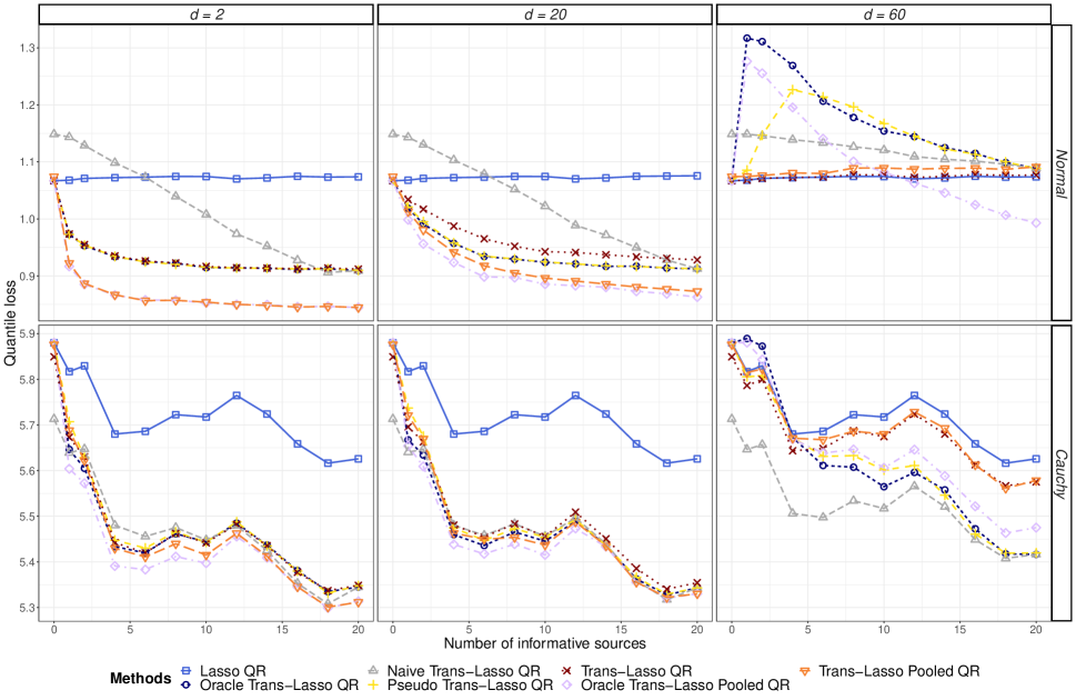
Figure 3: Average quantile loss among different $d$ with $\eta=20$ in homogeneous setting for normal and Cauchy error.

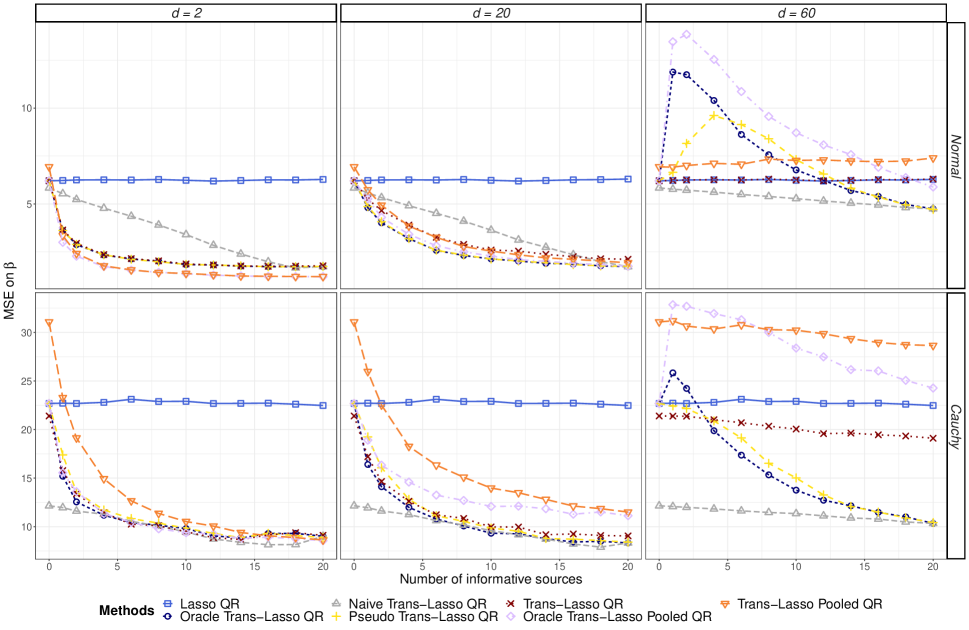
Figure 4: Average MSE on $\boldsymbol{\beta}$ among different $d$ with $\eta=20$ in homogeneous setting for normal and Cauchy error.

Figures 3-4 plot the QL values and the MSE values, respectively, for the cases with $p=150$ and $\eta=20$, averaged over replications. Detailed results are also shown in Tables B-B in the Appendix.

When $d=2$ or $d=20$, the informative sources are truly informative, as seen by the fact that all the transfer learning methods could greatly outperform Lasso QR, except for the naive approach. In these cases, the performance of both Trans-Lasso QR and Trans-Lasso Pooled QR closely aligns with their corresponding oracle procedures, affirming the efficacy of the informative source detection process. Interestingly, the pseudo Trans-Lasso QR, informed a priori about $|{\cal A}|$, performs comparably to the oracle. Conversely, the naive Trans-Lasso QR, which indiscriminately includes all sources, may underperform relative to Lasso QR when $|{\cal A}|$ is small.

When $d=60$, the informativeness of the sources diminishes, particularly in the normal residual setting, which is inherently simpler than the Cauchy residual setting. This is reflected in the performance of the oracle Trans-Lasso QR and oracle Trans-Lasso Pooled QR: under normal settings, they significantly underperform compared to Lasso QR with a small $|{\cal A}|$, but their performance incrementally improves as $|{\cal A}|$ increases, primarily due to the larger sample size of weakly informative samples. The pseudo Trans-Lasso QR exhibits similar behavior to the oracle, as it is constrained to use sources that are not genuinely informative. It is then interesting to see that the proposed Trans-Lasso QR method is very robust and performs as well as Lasso QR. The results show that the proposed informative source selection procedure works well; the Trans-Lasso QR is able to utilize the truly information sources to achieve positive transfer while not being misled by the “fake” informative sources that could cause negative transfer.

It is interesting to further compare Trans-Lasso QR and Trans-Lasso Pooled QR. In terms of the quantile loss, Trans-Lasso Pooled QR shows better performance than Trans-Lasso QR, especially under the normal residual setup with a small $d$ value. This is not surprising as the Trans-Lasso Pooled QR directly targets on the originally quantile loss. However, in terms of the MSE on $\boldsymbol{\beta}$, Trans-Lasso Pooled QR can be substantially outperformed by Trans-Lasso QR, especially in the Cauchy residual setup. This may be due to the instability or optimization issues with fitting the pooled sparse quantile regression models. We have also conducted additional simulation studies to compare their computational efficiency with large-scale problems. Specifically, consider the settings of Gaussian residuals, with $d=2$, $|{\mathcal{A}}|=10$, $p\in\{75,150,300,600\}$, and $n={n_{0}}=\cdots={n_{20}}\in\{1000,2500,5000,10000\}$. Figure 5 highlights the superior computational efficiency of Trans-Lasso QR over Trans-Lasso Pooled QR; the efficiency gain is consistent and substantial especially in large-scale settings with large $p$ and/or $n$. More detailed results are reported in Tables B-B in the Appendix.

We also observe that, as expected, in general all the methods perform better under normal error than under Cauchy error, and all the methods perform better with smaller $d$ and larger SNR; the different versions of transfer learning methods perform better with larger number of informative sources as long as $d$ is not too large.

To save space, we report the simulation results for $\eta\in\{5,10\}$ with normal residuals and $p\in\{75,225\}$ under $\eta=10$ in Tables B-B in the Appendix. The results indicate the superiority of the proposed approach under both low-dimension and high-dimension scenarios.

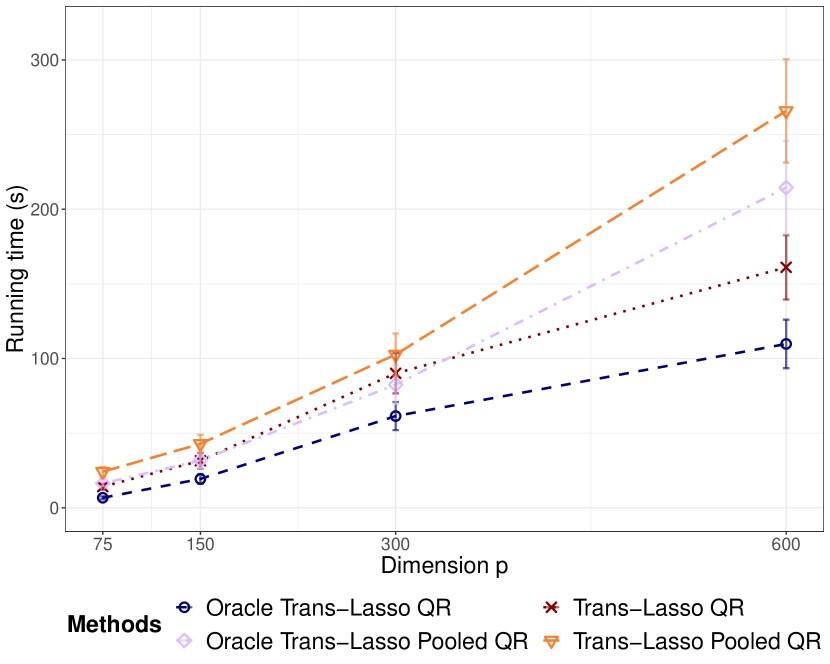
(a) Average running time comparison under $n=10000$ with different $p$

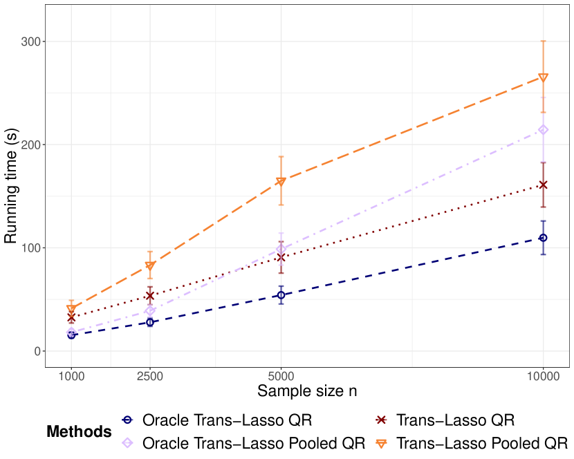
(b) Average running time comparison under $p=600$ with different $n$

Figure 5: Running time comparison between Trans-Lasso QR and Trans-Lasso Pooled QR. Each setting is replicated 100 times, and each error bar extends $\pm 1.96\times sd$ around the average. The experiment was run on a computational cluster with 4 Intel Xeon Gold 6230 CPUs at 2.10 GHz.

5.2 Heterogeneous Designs

We assume that the covariates from the target are generated from the Gaussian distribution with mean zero and the identity covariance matrix, and the covariates from the $k$th source are generated from the Gaussian distribution with mean zero and a covariance matrix with a Toeplitz structure

$$\boldsymbol{\Sigma}=\left({\begin{array}[]{*{20}{c}}{\begin{array}[]{*{20}{c}}{{\sigma_{0}}}&{{\sigma_{1}}}&{{\sigma_{2}}}\\ {{\sigma_{1}}}&{{\sigma_{0}}}&{{\sigma_{1}}}\\ {{\sigma_{2}}}&{{\sigma_{1}}}&{{\sigma_{0}}}\end{array}}&{\begin{array}[]{*{20}{c}}\cdots\\ {}\hfil\\ {}\hfil\end{array}}&{\begin{array}[]{*{20}{c}}{}\hfil&{{\sigma_{p-2}}}&{{\sigma_{p-1}}}\\ {}\hfil&{}\hfil&{{\sigma_{p-2}}}\\ {}\hfil&{}\hfil&{}\hfil\end{array}}\\ {\begin{array}[]{*{20}{c}}\vdots&}{\hfil&}{\hfil\end{array}}&\ddots&{\begin{array}[]{*{20}{c}}}{\hfil&}{\hfil&\vdots\end{array}}\\ {\begin{array}[]{*{20}{c}}{}\hfil&{}\hfil&{}\hfil\\ {{\sigma_{p-2}}}&{}\hfil&{}\hfil\\ {{\sigma_{p-1}}}&{{\sigma_{p-2}}}&{}\hfil\end{array}}&{\begin{array}[]{*{20}{c}}{}\hfil\\ {}\hfil\\ \cdots\end{array}}&{\begin{array}[]{*{20}{c}}{}\hfil&{}\hfil&{}\hfil\\ {}\hfil&{{\sigma_{0}}}&{{\sigma_{1}}}\\ {}\hfil&{{\sigma_{1}}}&{{\sigma_{0}}}\end{array}}\end{array}}\right).$$

with its first row given as

$$(\sigma_{0},\ldots,\sigma_{p-1})=({1,\underbrace{1/\left({k+1}\right),\ldots,1/\left({k+1}\right)}_{2k-1},{0_{p-2k}}}).$$

We refer to this as the “heterogeneous design” Scenario. The other settings are same as in Section 5.1.

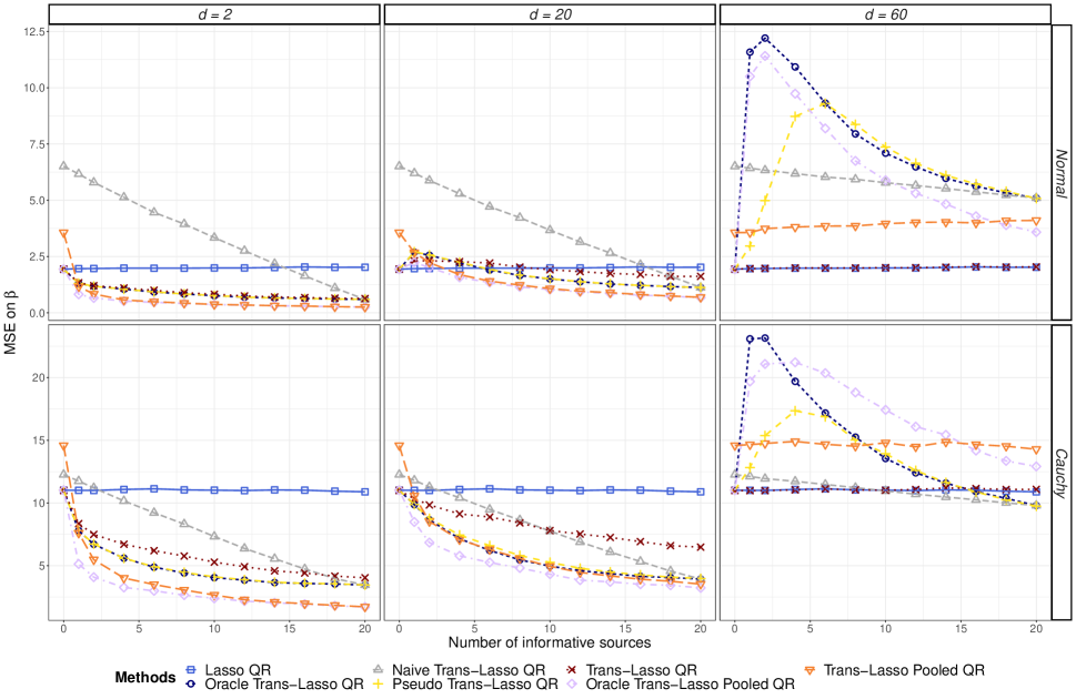
Figure 9: Average MSE on $\boldsymbol{\beta}$ among different $d$ with $\eta=20$ in heterogeneous setting for normal and Cauchy error.

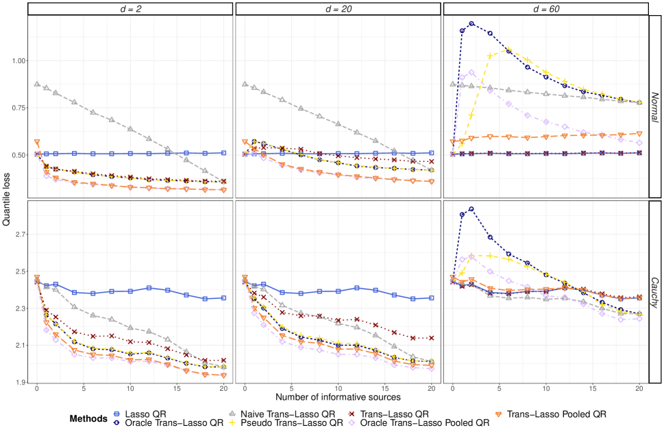
Figure 10: Average quantile loss among different $d$ with $\eta=20$ in heterogeneous setting for normal and Cauchy error.

The simulation results are reported in Figures 9-10 and Tables B-B in Appendix B. We omit detailed discussions as the main observations are consistent with those made in the homogeneous design scenario and with our theoretical results.

6 Application on Airplane Hard Landing

In aviation industry all over the world, quick access record (QAR) recorders are widely installed on aircraft to collect real-time data. With such real-time QAR data, statistical learning and machine learning approaches can be used to help prevent incidents during a flight’s most crucial time - approaching and landing. For example, Hong and Jun (2008) analyzed QAR data for fuel control, Lan et al. (2012) investigated QAR data for the safety of landing at high-attitude airports, and Sun and Xiao (2012) used QAR data to characterize pilots with their operations.

We study the risk of hard landing, i.e., high vertical acceleration at the touchdown point of a flight, with QAR data for 3 types of airplanes: Boeing 737 (B737), Airbus A320 (A320), and Airbus A380 (A380). The maximum vertical acceleration (MVA) during landing is a commonly-used standard to measure the loading during landing (Wang et al., 2014; Qian et al., 2017), so it can serve as a numerical proxy of the risk of hard landing and is used as the response variable in our study. The sensors on the airplane record 15 flight attributes during the flight, including Airspeed, Altitude, Bank Angle, Flap Angle, Gross Weight, Ground Speed, Wind Speed and Direction, Stabilizer Angle, Temperature, Fuel Consumption, Fuel Flow, and the Acceleration. In our study, the covariates consist of these attributes measured at several critical time points before or during the landing procedure, as well as various summary statistics (average, max, etc) of these attributes computed for different phases of a flight. A full list of the covariates is provided in Section C in the Appendix. Indeed, previous catastrophes indicate that there exist strong linkages between the MVA (or the loading on the landing gear) and some flight attributes captured in QAR. For instance, in 1992, Martinair Flight 495 crashed on its landing runway with a high loading partially because of the low airspeed caused by a micro-burst.

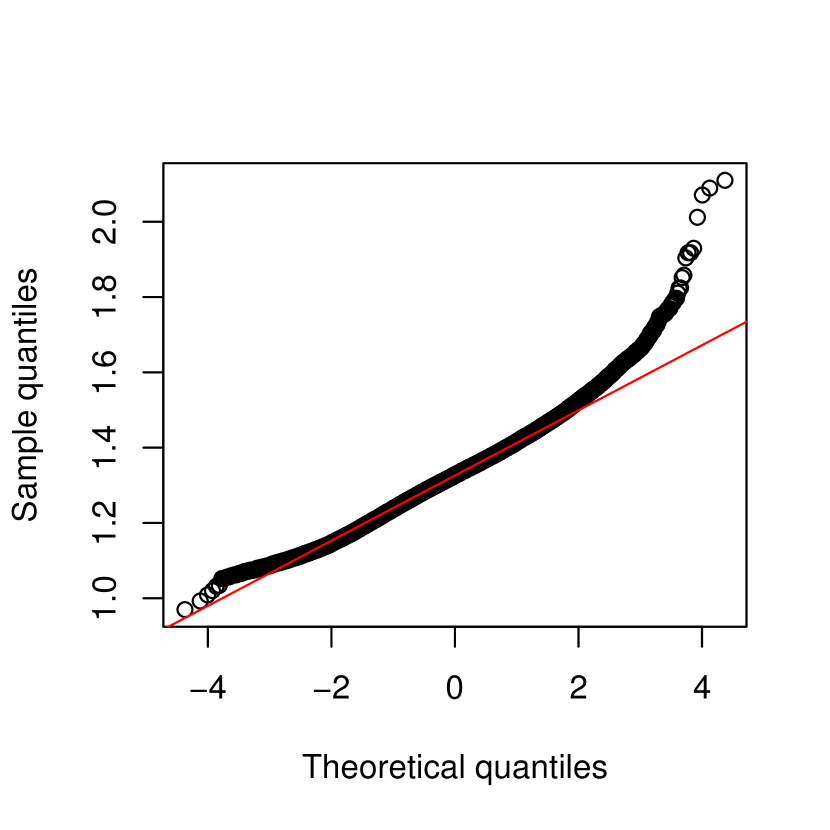
(a) Normal Q-Q plot for the MVA from Airbus 320 records.

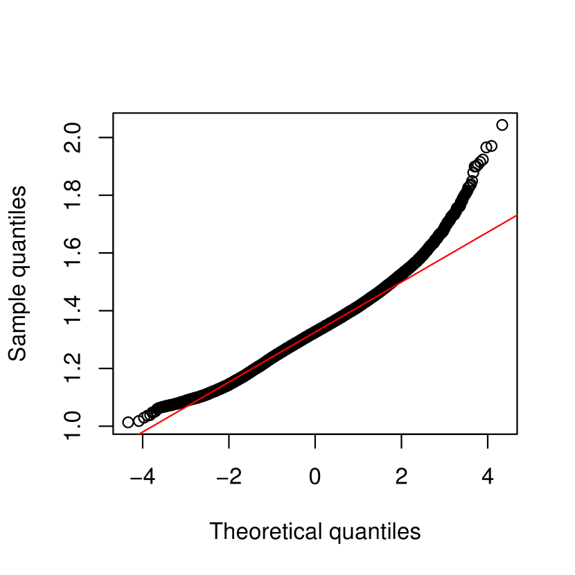
(b) Normal Q-Q plot for the MVA from Boeing 737 records.

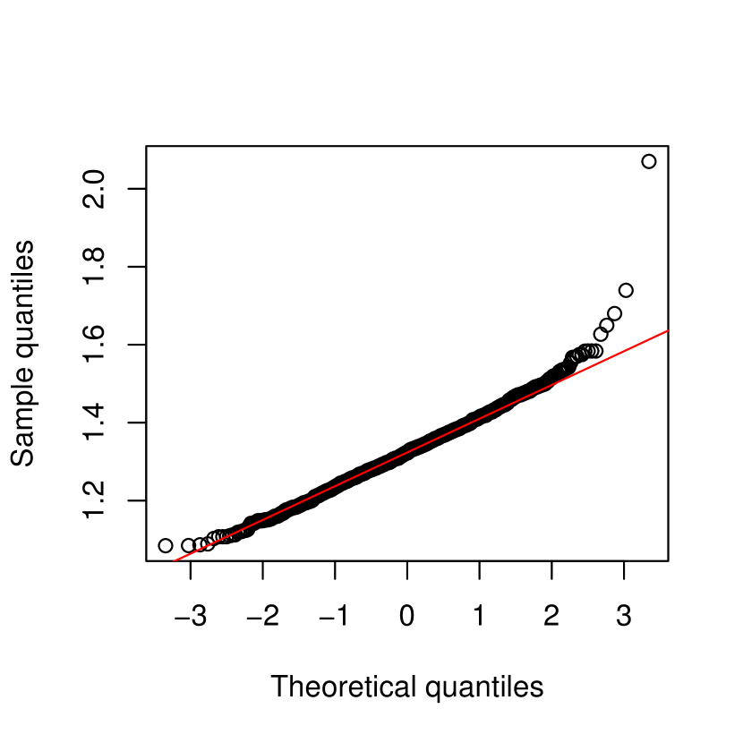
(c) Normal Q-Q plot for the MVA from Airbus 380 records.

Figure 12: Evidences that the MVA are highly right skewed and further are not in normal distribution.

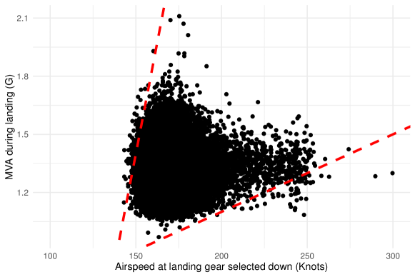
Figure 13: Heteroscedasticity of MVA with respect of Airspeed at Landing Gear Selected Down in Airbus 320 dataset.

To study the associations between the MVA and the flight attributes, quantile regression is more suitable than mean regression for various reasons. First, we mainly concern those high-risk flights with higher than usual MVA values. Second, the empirical distribution of MVA is generally highly right skewed as seen from Figure 12 in the Appendix, which may make the normality assumption in mean regression models inappropriate. Another reason is that the associations between flight attributes and the MVA often exhibit heteroscedasticity; see Figure 13 in the Appendix for an example. However, existing works on modeling the hard landing with QAR data take a target-only modeling approach by focusing on a single type of aircraft (Qian et al., 2017) or a one-size-fits-all approach by modeling all types of aircraft together (Chen and Jin, 2021).

We apply the proposed transfer learning approaches to perform quantile regression analyses of the MVA on the QAR features at $\tau=0.9$, for three types of flights, namely, Boeing 737 (B737), Airbus A320 (A320), and Airbus A380 (A380). We consider each of the three types of airplanes as the target and the rest two types as the sources. Under each of the three settings, we randomly split the target data to 80% training and 20% testing. All the features are standardized within each dataset prior to performing the train-test split. The training data are used to fit QR models and the tuning parameters are selected by the cross validation procedure as described in Section 5. The testing data are then used to evaluate the final tuned models. We consider Lasso QR, the Naive Trans-Lasso QR (assuming that all sources are informative), and the proposed Trans-Lasso QR methods. For the case that A380 is the target, we have also fitted transfer learning models with all different choices of informative set. The random splitting procedure is repeated 20 times under each setting, from which we compute the means and the standard deviations of the out-of-sample quantile loss values for different methods.

Figure 6(a) shows the results of the out-of-sample quantile loss values for the three settings of different targets. For each bar, its height represents the average quantile loss value and its error bar extends two standard deviations to indicate how the individual loss values are dispersed around the average. The Trans-Lasso QR method is the most beneficial for modeling A380 as the target, where it leads to substantially lower quantile loss than Lasso QR and Naive Trans-Lasso QR. This may be due to the fact that the sample size for A380 is quite low so it is crucial to borrow information from other similar types of flights. Indeed, the number of flight records for A380 is around 10,000, which is much smaller than that of B737 and A320, which exceed 630,000. On the other hand, neither B737 nor A320 appears to benefit from transfer learning, as the sample size for each type is already quite adequate. Nevertheless, the performance of Trans-Lasso QR is at least comparable to Lasso QR and is always slightly better than Naive Trans-Lasso QR, which suggests that Trans-Lasso QR is quite robust and can avoid negative transfer with data-driven informative set selection.

Figure 6(b) shows the results of using different informative sets for the case that A380 is the target. Very interestingly, the results suggest that using A320 as the single informative set leads to the best transfer learning model for A380. By cross referencing the two figures, it can be seen that this informative set is also the one selected by the proposed Trans-Lasso QR method. Indeed, A380 is more similar to A320 than to B737 since the former two are essentially cousins from the same company. The Boeing series aircrafts adopt the control wheel and control column to operate, while the Airbus aircrafts are equipped with the control stick. With a control stick that uses wire technology, the operating commands are delivered to the computer for translation and assignment, however, with the control wheel and column, the signal is delivered physically, and it directly connects with all the control surfaces including several flaps, slats, stabilizers, etc. See Tomczyk (2002) and Filburn (2020) for more discussions about this topic. This difference in operating mechanisms may lead to the difference in landing performance under even the same external conditions, making A320 a more informative source than B737 to A380.

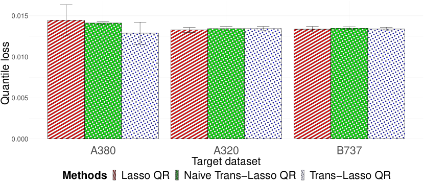
(a) Quantile loss on different selected target datasets with different algorithms.

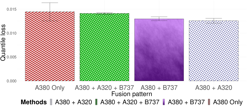
(b) Quantile loss on A380 as the target with all different fusion combinations.

Figure 6: Performances comparison for the hard landing analysis with given quantile level $\tau=0.9$.

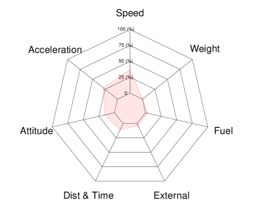
Figure 7: Radar plot for categorized feature contribution from A380 Tran-Lasso QR with $\tau=0.9$.

To gain more insights on the risk factors of hard landing for A380, we categorize all features and quantify their group-level relative contributions to the MVA, based on the fitted Trans-Lasso QR model with A380 being the target. Specifically, all features are categorized into seven categories: Speed, Fuel (consumption), Distance and Time, Acceleration (non-vertical), Weight, Attitude, and External. The detailed categorization is provided by the “Type” column of the feature table in Appendix C. To measure the contribution of each category of features, we compute the sum of the absolute values of their estimated coefficients. These measures from different feature categories are then divided by the total contributions from all the categories to make them summing up as $1$ and become a set of relative contributions within $\left[{0,1}\right]$. Figure 7 visualizes the relative contributions of the seven feature categories using a radar plot. We can see that speed, acceleration and attitude measurements appear to be the more relevant to the hard landing risk. Interesting, many features in these three categories could potentially be controlled or altered by the pilot team in normal circumstances, while the features in the other three of four categories, namely, fuel, weight, and external measurements, arguably, are mostly external and “uncontrollable”. As such, the results suggest that it is hopeful to reduce the risk of hard landing by minimizing the bad impact or maximizing the good impact from the controllable “human factors”. In other words, training better pilots may be the most important.

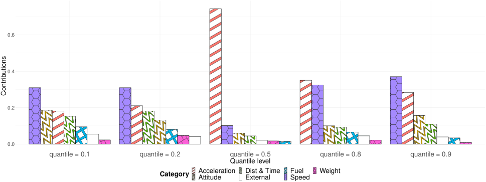
Figure 8: Barplot of relative contributions of seven feature categories from A380 Trans-Lasso QR models with varying quantile levels.

It is also interesting to compare the risk factors for hard landing across quantile levels. We thus apply the Trans-Lasso QR with A380 being the target under three quantile levels, namely, $\tau\in\{0.1,0.2,0.5,0.8,0.9\}$, where $\tau\in\{0.1,0.2\}$ represent good landing, $\tau=0.5$ represents normal landing, and $\tau\in\{0.8,0.9\}$ represent hard landing. Figure 8 show the comparison of the relative contributions of the risk factors from the fitted models with different quantile levels. There are several interesting observation. The three controllable or human risk factors, namely, speed, acceleration, and attitude, are always among the most important factors, and their overall importance tends to be higher with the deterioration of the quality of landing. For good landings, the “External” factor also plays an important role besides the three human factors. For normal landing, the acceleration factor stands out as a single most important factor, while for hard landing, both acceleration and speed become important. This suggests that hard landing is more likely to occur when both acceleration and speed go wrong.

7 Discussion

We have developed Trans-Lasso QR, to enable transfer learning for fitting high-dimensional quantile regression. Our method utilizes the idea of response surrogation to simplify the quantile loss and the idea of sampling splitting to distinguish informative sources for ensuring positive transfer. With QAR data, we are able to build an improved quantile regression models for the landing load of A380 airplane with the help from A320 and B737.

There are several directions for future research. A potential extension is to investigate transfer learning for binary quantile regression through latent variable models, which may be preferred in modeling rare events with highly sparse binary outcomes. Moreover, it is interesting to consider the scenario of multiple targets, and how to fit multiple or multivariate transfer learning models in a collaborative fashion remains a challenging yet rewarding problem. Furthermore, enabling transfer learning of quantile regression without pooling raw data from the sources to the target could be very useful; this “transfer learning without transfer” approach would leverage the benefits of integrative learning while minimizing the need of data integration and preserving the confidentiality of individual sources. Another interesting problem is to utilize the composite quantile regression framework (Zou and Yuan, 2008) under the transfer learning setup. We will also exploring the connections between transfer learning and hierarchical Bayesian modeling (Karbalayghareh et al., 2018), and apply the proposed approach to tackle more real-world problems in engineering and public health to better utilize data from disparate sources.

Appendix A Proofs

A.1 Proofs of Theorem 4.1

We acknowledge that the proof of Theorem 4.1 follows similar structure as those of Theorem 1 and Theorem 4 in Li et al. (2021), and the main challenge is to handle the quantile loss via a surrogate response (Chen et al., 2020). For the sake of completeness, we still present the relevant materials and results from existing works that are adapted to our setting. For simplicity, we do not use different notations for the constants appear in rates or probability expressions. For example, we always use $c_{1}$ to describe any constants in probability expressions like $1-\exp\{-c_{1}n_{0}\}$.

Lemma A.1 (Proposition 11 in Chen et al. (2020)).

Denote ${\widehat{\boldsymbol{\Sigma}}{}^{(k)}}=\sum\nolimits_{i=1}^{{n_{k}}}{{\boldsymbol{X}^{(k)}}^{\top}}{\boldsymbol{X}^{(k)}}/{n_{k}}$ for $k=0,\ldots,K$. Recall ${{\widetilde{\boldsymbol{y}}}^{(k)}}$ is the surrogate response as defined in (7) of the main paper. Under Assumption 1, 2, 4, 5 and 6, for any $k=0,\ldots,K$, we have

$${{\left\|{\frac{1}{n_{k}}{\boldsymbol{X}^{\left(k\right)^{\top}}}{{\widetilde{\boldsymbol{y}}}^{\left(k\right)}}-{\widehat{\boldsymbol{\Sigma}}{}^{\left(k\right)}}{\boldsymbol{\beta}^{\left(k\right)}}}\right\|}_{\infty}}\lesssim\sqrt{\frac{{\log\left({p\vee{n_{k}}}\right)}}{{{n_{k}}}}}+\frac{{{s_{k}}\log\left({p\vee{n_{k}}}\right)}}{{{n_{k}}}}.$$

with probability at least $1-c_{1}n_{k}^{-c_{2}s_{k}}-c_{3}\exp({-{c_{4}}{n_{k}}})$ for positive constants ${c_{1}}$ to ${c_{4}}$.

Remark.

The Assumption 1 is necessary here by noticing that following the proof of Proposition 11 in Chen et al. (2020) will lead to

$${{\left\|{\frac{1}{n_{k}}{\boldsymbol{X}^{\left(k\right)^{\top}}}{{\widetilde{\boldsymbol{y}}}^{\left(k\right)}}-{\widehat{\boldsymbol{\Sigma}}{}^{\left(k\right)}}{\boldsymbol{\beta}^{\left(k\right)}}}\right\|}_{\infty}}\lesssim\sqrt{\frac{{\log p}}{{{n_{k}}}}}+\sqrt{\frac{{{s_{k}}{a_{n}}\log{n_{k}}}}{{{n_{k}}}}}+a_{n}^{2},$$

where ${a_{n}}=\sqrt{{s_{k}}\log{n_{k}}/{n_{k}}}$ is the convergence rate of the initial estimator of $\boldsymbol{\beta}_{k}$. As such, to obtain the desired rate in Lemma S.1, we need ${s_{k}}{a_{n}}=O(1)$, i.e., $\sqrt{s_{k}^{3}\log{n_{k}}/{n_{k}}}=O(1)$, which requires $s_{k}=O({n_{k}^{r}})$ with $r\in({0,1/3})$ as shown in Assumption 1.

The Assumption 4 (Irrepresentable condition) is also necessary here to control the error of estimating the error density functions, which is preliminary for this Lemma A.1.

Namely, with ${{\widehat{f}}^{(k)}}(0)$ defined in Equation 6, Assumption 4 contributes to obtain

$$\left|{{{\widehat{f}}^{\left(k\right)}}\left(0\right)-{f^{\left(k\right)}}\left(0\right)}\right|=O\left({\sqrt{\frac{{{s_{k}}\log{n_{k}}}}{{{n_{k}}{h^{\left(k\right)}}}}}+\sqrt{\frac{{{s_{k}}\log{n_{k}}}}{{{n_{k}}}}}}\right).$$

Specifically, denote

$$D_{n,{h^{\left(k\right)}}}^{\left(k\right)}\left(\boldsymbol{\beta}\right)=\frac{1}{{n{h^{\left(k\right)}}}}\sum\limits_{i=1}^{{n_{k}}}{G\left({\frac{{y_{i}^{\left(k\right)}-\boldsymbol{x}_{i,{S_{k}}}^{\left(k\right)^{\top}}{\boldsymbol{\beta}_{{S_{k}}}}}}{{{h^{\left(k\right)}}}}}\right)},$$

in which $\boldsymbol{x}_{i}^{(k)^{\top}}{\widehat{\boldsymbol{\beta}}{}^{(k)}}$ is replaced by $\boldsymbol{x}_{i,{S_{k}}}^{(k)^{\top}}{\boldsymbol{\beta}_{{S_{k}}}}$. If ${{\hat{S}}_{k}}\subseteq{S_{k}}$ holds true with high probability (for which we would need the irrepresentable condition), then we have ${{{\widehat{f}}^{(k)}}(0)=D_{n,{h^{(k)}}}^{(k)}({{{\hat{\boldsymbol{\beta}}}^{(k)}}})}$ with high probability and can bound $|{{{\widehat{f}}^{(k)}}(0)-{f^{(k)}}(0)}|$ by

$$\left|{{{\widehat{f}}^{\left(k\right)}}\left(0\right)-{f^{\left(k\right)}}\left(0\right)}\right|\leq\mathop{\sup}\limits_{\left\|{{\boldsymbol{\beta}_{{S_{k}}}}-\boldsymbol{\beta}_{{S_{k}}}^{\left(k\right)}}\right\|\leq{a_{n}}}\left|{D_{n,{h^{\left(k\right)}}}^{\left(k\right)}\left(\boldsymbol{\beta}\right)-{f^{\left(k\right)}}\left(0\right)}\right|,$$

where ${a_{n}}={\sqrt{s_{k}\log n_{k}/n_{k}}}$ is the convergence rate of the initial estimator of $\boldsymbol{\beta}_{k}$ provided by Fan et al. (2014).

The main consequence, as shown in Chen et al. (2020), is that the estimation of the density only relies on the $s_{k}$ dimensions of the initial estimator, not all the $p$ dimensions, which facilitates the next step of using sub-interval cutting technique on each dimension to further bound the error of estimating the error density. That is, for each dimension $i$ in the support index $S_{k}$, we divide the interval $[{\beta_{i}^{(k)}-{a_{n}},\beta_{i}^{(k)}+{a_{n}}}]$ into $n^{M}$ small subintervals and each has length $2{a_{n}}/{n^{M}}$, forming a set of points $\{{{\boldsymbol{\beta}_{j}},1\leq j\leq{q_{n}}}\}$ in ${\mathbb{R}^{p}}$ with cardinality ${q_{n}}\leq{n^{M{s_{k}}}}$ such that for any $\boldsymbol{\beta}$ in the ball $\|{{\boldsymbol{\beta}_{{S_{k}}}}-\boldsymbol{\beta}_{{S_{k}}}^{(k)}}\|\leq{a_{n}}$, we have $\|{{\boldsymbol{\beta}_{{S_{k}}}}-\boldsymbol{\beta}_{j,{S_{k}}}^{(k)}}\|\leq 2\sqrt{{s_{k}}}{a_{n}}/{n^{M}}$ for some $1\leq j\leq{q_{n}}$ and $\|{{\boldsymbol{\beta}_{j,{S_{k}}}}-\boldsymbol{\beta}_{{S_{k}}}^{(k)}}\|\leq{a_{n}}$. Hence, we can further link ${\sup_{\|{{\boldsymbol{\beta}_{{S_{k}}}}-\boldsymbol{\beta}_{{S_{k}}}^{(k)}}\|\leq{a_{n}}}}|{D_{n,{h^{(k)}}}^{(k)}(\boldsymbol{\beta})-{f^{(k)}}(0)}|$ with ${\sup_{1\leq j\leq{n^{M{s_{k}}}}}}|{D_{n,{h^{(k)}}}^{(k)}({{\boldsymbol{\beta}_{j}}})-{f^{(k)}}(0)}|$ and bound the later one with the help of the exponential inequality. This leads to the desired bound for the error of estimating density functions.

Lemma A.2 (Theorem 1 in Raskutti et al. (2010)).

Denote ${\widehat{\boldsymbol{\Sigma}}{}^{\cal A}}=\sum\nolimits_{k\in{\cal A}\cup\{0\}}{{\alpha_{k}}{\widehat{\boldsymbol{\Sigma}}{}^{(k)}}}$, ${\boldsymbol{\Sigma}^{\cal A}}=\sum\nolimits_{k\in{\cal A}\cup\{0\}}{{\alpha_{k}}{\boldsymbol{\Sigma}^{(k)}}}$ and ${\rho^{2}}(\boldsymbol{\Sigma})=\mathop{\max}\limits_{j=1,\ldots,p}{\Sigma_{j,j}}$. Under Assumption 2, we have

$${u^{\top}}{\widehat{\boldsymbol{\Sigma}}{}^{\cal A}}u\geq\frac{1}{32}{u^{\top}}{\boldsymbol{\Sigma}^{\cal A}}u-81{\rho^{2}}\left(\boldsymbol{\Sigma}^{\cal A}\right)\frac{{\log p}}{n_{\cal A}+n_{0}}\left\|u\right\|_{1}^{2}$$

for any $u\in{{\mathbb{R}}^{p}}$ with probability at least $1-\exp({-{c_{1}}{({n_{\cal A}}+n_{0})}})$ and

$${u^{\top}}{\widehat{\boldsymbol{\Sigma}}{}^{\left(0\right)}}u\geq\frac{1}{32}{u^{\top}}{\boldsymbol{\Sigma}^{\left(0\right)}}u-81{\rho^{2}}\left({\boldsymbol{\Sigma}^{\left(0\right)}}\right)\frac{{\log p}}{n_{0}}\left\|u\right\|_{1}^{2}$$

for any $u\in{{\mathbb{R}}^{p}}$ with probability at least $1-\exp({-{c_{1}}{n_{0}}})$ for positive constant ${c_{1}}$.

Lemma A.3 (Bernstein’s inequality (Theorem 1.13 of Rigollet and Hütter (2015))).

We say a random variable $X$ follows a sub-exponential distribution with parameter $\lambda$ (denoted as $X\sim subE(\lambda)$) if ${\mathbb{E}}[X]=0$ and its moment generating function satisfies

$${\mathbb{E}}\left[{{e^{sX}}}\right]\leq\exp\left({\frac{1}{2}{s^{2}}{\lambda^{2}}}\right),\begin{array}[]{*{20}{c}}{}\hfil&{\forall\left|s\right|\leq\frac{1}{\lambda}}.\end{array}$$

If ${X_{1}},\ldots,{X_{n}}$ are independent random variables with ${\mathbb{E}}{X_{i}}={\mu_{i}}$ and ${X_{i}}-{\mu_{i}}\sim subE({\lambda})$, then for any $t>0$ we have

$${\mathbb{P}}\left({\frac{1}{n}\left|{\sum\limits_{i=1}^{n}{\left({{X_{i}}-{\mu_{i}}}\right)}}\right|\geq t}\right)\leq\exp\left({-\frac{n}{2}\min\left\{{\frac{{{t^{2}}}}{\lambda^{2}},\frac{t}{\lambda}}\right\}}\right).$$

We now give the outline of proving Theorem 4.1, followed by detailed derivations. Denote ${\boldsymbol{\beta}^{\cal A}}$ as the probabilistic limit of ${\widehat{\boldsymbol{\beta}}{}^{\cal A}}$ in Step 3 of the oracle algorithm, which is the solution of the following moment equation

$${\mathbb{E}}\left[{\sum\limits_{k\in{{\cal A}}\cup\left\{0\right\}}{{{\left({{\boldsymbol{X}^{\left(k\right)}}}\right)}^{\top}}\left({{{\tilde{y}}^{\left(k\right)}}-{\boldsymbol{X}^{\left(k\right)}}{\boldsymbol{\beta}^{{\cal A}}}}\right)}}\right]=0,$$ (17)

where $\widetilde{y}^{(k)}={\boldsymbol{x}^{(k)^{\top}}}{\boldsymbol{\beta}^{(k)}}-\{{f^{(k)}}(0)\}^{-1}\{{I({y^{(k)}-{\boldsymbol{x}^{(k)^{\top}}}{\boldsymbol{\beta}^{(k}}\leq 0})-\tau}\}.$ Thus, ${\boldsymbol{\beta}^{{\cal A}}}$ has the explicit form as ${\boldsymbol{\beta}^{\cal A}}={\boldsymbol{\beta}^{(0)}}+{\boldsymbol{\delta}^{\cal A}}$, where ${\boldsymbol{\delta}^{\cal A}}={({{\boldsymbol{\Sigma}^{\cal A}}})^{-1}}\sum_{k\in{\cal A}\cup\{0\}}{{\alpha_{k}}{\boldsymbol{\Sigma}^{(k)}}{\boldsymbol{\delta}^{(k)}}}$. It implies ${\boldsymbol{\beta}^{{\cal A}}}$ is a pooled version of ${\boldsymbol{\beta}^{(0)}}$ and ${\boldsymbol{\beta}^{(k)}}$ for all $k\in{\cal A}$ such that ${\boldsymbol{\beta}^{\cal A}}={({{\boldsymbol{\Sigma}^{\cal A}}})^{-1}}\sum_{k\in{\cal A}\cup\{0\}}{{\alpha_{k}}{\boldsymbol{\Sigma}^{(k)}}{\boldsymbol{\beta}^{(k)}}}$. Define

$${E_{1}}=\, \left\{{\frac{1}{{{n_{\cal A}}+{n_{0}}}}{\left\|\sum\limits_{k\in{\cal A}\cup\left\{0\right\}}{{{{\boldsymbol{X}^{(k)^{\top}}}}}({{\widetilde{\boldsymbol{y}}}^{(k)}-\boldsymbol{X}^{(k)}{\boldsymbol{\beta}^{\mathcal{A}}}})}\right\|_{\infty}}\leq\frac{{{\lambda_{1}}}}{2}}\right\},$$

$$E_{2}=\, \left\{{\frac{1}{{{n_{0}}}}\left\|{{{\boldsymbol{X}^{(0)^{\top}}}}}\left({{\widetilde{\boldsymbol{y}}}^{(0)}-\boldsymbol{X}^{(0)}{\boldsymbol{\beta}^{\left(0\right)}}}\right)\right\|_{\infty}\leq\frac{{{\lambda_{2}}}}{2}}\right\}.$$

We will show the following statements:

• (i) Denote ${\widehat{\boldsymbol{u}}{}^{\cal A}}=\widehat{\boldsymbol{\beta}}{}^{{\cal A}}-\boldsymbol{\beta}^{{\cal A}}$. On the event of $E_{1}$, we have

  $$\widehat{\boldsymbol{u}}{}^{{\cal A}^{\top}}\widehat{\boldsymbol{\Sigma}}{}^{\cal A}\widehat{\boldsymbol{u}}{}^{\cal A}\vee{\left\|{\widehat{\boldsymbol{u}}{}^{\cal A}}\right\|^{2}}\lesssim\, {{s_{0}}\lambda_{1}^{2}+{\lambda_{1}}C_{\boldsymbol{\Sigma}}^{\cal A}d},$$

  $$\left\|{\widehat{\boldsymbol{u}}{}^{\cal A}}\right\|_{1}\lesssim\, {{s_{0}}{\lambda_{1}}+C_{\boldsymbol{\Sigma}}^{\cal A}d}$$

  with probability at least $1-\exp({-c_{1}{({n_{\cal A}}+n_{0})}})$.

• (ii) Denote ${\widehat{\boldsymbol{v}}{}^{\cal A}}=\widehat{\boldsymbol{\delta}}{}^{\cal A}-\boldsymbol{\delta}^{\cal A}$. On the event of $E_{2}$, we have

  $${\widehat{\boldsymbol{u}}{}^{{\cal A}^{\top}}}{{\widehat{\boldsymbol{\Sigma}}{}}^{\left(0\right)}}{\widehat{\boldsymbol{u}}{}^{\cal A}}\vee{\left\|{{\widehat{\boldsymbol{v}}{}^{\cal A}}}\right\|^{2}}\lesssim\, {s_{0}\lambda_{1}^{2}+{\lambda_{1}}C_{\boldsymbol{\Sigma}}^{\cal A}d},$$

  $${{\widehat{\boldsymbol{v}}{}^{{\cal A}}}^{\top}}{\widehat{\boldsymbol{\Sigma}}{}^{\left(0\right)}}{\widehat{\boldsymbol{v}}{}^{\cal A}}\lesssim\, {{\lambda_{2}}C_{\boldsymbol{\Sigma}}^{\cal A}d},$$

  $${\left\|{{{\widehat{\boldsymbol{v}}{}}^{\cal A}}}\right\|^{2}}\lesssim\, {{\lambda_{2}}C_{\boldsymbol{\Sigma}}^{\cal A}d\wedge{{\left({C_{\boldsymbol{\Sigma}}^{\cal A}d}\right)}^{2}}}$$

  with probability at least $1-3\exp({-c_{1}{n_{0}}})$.

We will then show that ${\mathbb{P}}\left({{E_{1}}\cap{E_{2}}}\right)\rightarrow 1$ as $p\rightarrow\infty$ and ${\underline{n}_{{\cal A}}}\rightarrow\infty$, where ${\underline{n}_{{\cal A}}}=\mathop{\min}\limits_{k\in{\cal A}\cup\left\{0\right\}}{n_{k}}$ is the minimum sample size among informative sources and the target. Finally, the proof of Theorem 4.1 is completed by utilizing Lemma A.2 and the fact that

$$\left\|{\widehat{\boldsymbol{\beta}}{}-{\boldsymbol{\beta}^{\left(0\right)}}}\right\|=\, \left\|{\left({{\widehat{\boldsymbol{\beta}}{}^{\cal A}}-{\widehat{\boldsymbol{\delta}}{}^{\cal A}}}\right)-\left({{\boldsymbol{\beta}^{\cal A}}-{\boldsymbol{\delta}^{\cal A}}}\right)}\right\|$$

$$\leq\, \left\|{\widehat{\boldsymbol{u}}{}^{\cal A}}\right\|+\left\|{\widehat{\boldsymbol{v}}{}^{\cal A}}\right\|.$$

We now prove statement (i). We have the following oracle inequality, the same as (A.1) in the supplementary material of Li et al. (2021). For simplicity of the notation, we denote $S={S_{0}}$. By applying Taylor expansion on the loss function in (8),

$$\frac{1}{2}{\widehat{\boldsymbol{u}}{}^{{\cal A}^{\top}}}\widehat{\boldsymbol{\Sigma}}{}^{\cal A}\widehat{\boldsymbol{u}}{}^{\cal A}$$

$$\leq\, {\lambda_{1}}\left\|\boldsymbol{\beta}^{{\cal A}}\right\|_{1}-{\lambda_{1}}\left\|\widehat{\boldsymbol{\beta}}{}^{\cal A}\right\|_{1}+\left|\frac{{{{{\widehat{\boldsymbol{u}}{}^{{\cal A}^{\top}}}}}}}{{\left({{n_{\cal A}}+{n_{0}}}\right)}}\sum\limits_{k\in{\cal A}\cup\left\{0\right\}}{{{{\boldsymbol{X}^{(k)^{\top}}}}}\left({{\widetilde{\boldsymbol{y}}}^{(k)}-\boldsymbol{X}^{(k)}\boldsymbol{\beta}^{{\cal A}}}\right)}\right|$$

$$\leq\, {\lambda_{1}}\left\|\boldsymbol{\beta}^{{\cal A}}\right\|_{1}-{\lambda_{1}}\left\|\widehat{\boldsymbol{\beta}}{}^{{\cal A}}\right\|_{1}+\frac{{{\lambda_{1}}}}{2}\left\|\widehat{\boldsymbol{u}}{}^{{\cal A}}\right\|_{1}$$

$$\leq\, \frac{3}{2}{\lambda_{1}}{\left\|{\widehat{\boldsymbol{u}}{}_{S}^{\cal A}}\right\|_{1}}+{\lambda_{1}}{\left\|{\boldsymbol{\beta}_{{S^{c}}}^{\cal A}}\right\|_{1}}-{\lambda_{1}}{\left\|{\widehat{\boldsymbol{\beta}}{}_{{S^{c}}}^{\cal A}}\right\|_{1}}+\frac{1}{2}{\lambda_{1}}{\left\|{\widehat{\boldsymbol{u}}{}_{{S^{c}}}^{\cal A}}\right\|_{1}}$$

$$\leq\, \frac{3}{2}{\lambda_{1}}{\left\|{\widehat{\boldsymbol{u}}{}_{S}^{\cal A}}\right\|_{1}}+\frac{3}{2}{\lambda_{1}}{\left\|{\boldsymbol{\beta}_{{S^{c}}}^{\cal A}}\right\|_{1}}-\frac{1}{2}{\lambda_{1}}{\left\|{\widehat{\boldsymbol{u}}{}_{{S^{c}}}^{\cal A}}\right\|_{1}},$$

where the third line holds true due to event $E_{1}$ and Hölder’s inequality, the fourth line holds true due to ${\|{\widehat{\boldsymbol{\beta}}{}_{S}^{\cal A}-\boldsymbol{\beta}_{S}^{\cal A}}\|_{1}}\geq{\|{\widehat{\boldsymbol{\beta}}{}_{S}^{\cal A}}\|_{1}}-{\|{\boldsymbol{\beta}_{S}^{\cal A}}\|_{1}}$, and the last line holds true due to ${\|{\widehat{\boldsymbol{u}}{}_{{S^{c}}}^{\cal A}}\|_{1}}\leq{\|{\widehat{\boldsymbol{\beta}}{}_{{S^{c}}}^{\cal A}}\|_{1}}+{\|{\boldsymbol{\beta}_{{S^{c}}}^{\cal A}}\|_{1}}$.

If ${\|{\widehat{\boldsymbol{u}}{}_{S}^{\cal A}}\|_{1}}\geq{\|{\boldsymbol{\beta}_{{S^{c}}}^{\cal A}}\|_{1}}$, with a positive constant $c_{4}$, we can further have

$${\left\|{{\widehat{\boldsymbol{u}}{}^{\cal A}}}\right\|^{2}}-\frac{{\log p}}{{{n_{\cal A}}+{n_{0}}}}\left\|{{\widehat{\boldsymbol{u}}{}^{\cal A}}}\right\|_{1}^{2}\lesssim\, \frac{1}{2}{\widehat{\boldsymbol{u}}{}^{{\cal A}^{\top}}}\widehat{\boldsymbol{\Sigma}}{}^{\cal A}\widehat{\boldsymbol{u}}{}^{\cal A}$$

$$\leq\, 3{\lambda_{1}}{\left\|{\widehat{\boldsymbol{u}}{}_{S}^{\cal A}}\right\|_{1}}-\frac{1}{2}{\lambda_{1}}{\left\|{\widehat{\boldsymbol{u}}{}_{{S^{c}}}^{\cal A}}\right\|_{1}}$$

$$\leq\, 3{\lambda_{1}}{\left\|{\widehat{\boldsymbol{u}}{}_{S}^{\cal A}}\right\|_{1}}$$

$$\leq\, 3{\lambda_{1}}\sqrt{{s_{0}}}{\left\|{\widehat{\boldsymbol{u}}{}_{S}^{\cal A}}\right\|}$$

$$\leq\, 3{\lambda_{1}}\sqrt{{s_{0}}}{\left\|{\widehat{\boldsymbol{u}}{}^{\cal A}}\right\|},$$

where the first line holds true with probability at least $1-\exp({-{c_{1}}{({n_{\cal A}}+n_{0})}})$ due to Lemma A.2 and Assumption 4, and the fourth line holds true due to $\ell_{1}$-$\ell_{2}$ inequality. It further leads to

$${\left\|{\widehat{\boldsymbol{u}}{}^{\cal A}}\right\|^{2}}\lesssim\, {s_{0}\lambda_{1}^{2}},$$ (18)

$${\left\|{\widehat{\boldsymbol{u}}{}^{\cal A}}\right\|_{1}}\lesssim\, {s_{0}{\lambda_{1}}}$$ (19)

by utilizing ${s_{0}}\log p/({{n_{\cal A}}+{n_{0}}})=o(1)$ derived from Assumption 3.

On the other hand, if ${\|{\widehat{\boldsymbol{u}}{}_{S}^{\cal A}}\|_{1}}\leq{\|{\boldsymbol{\beta}_{{S^{c}}}^{\cal A}}\|_{1}}$, we have

$$0\leq\frac{1}{2}{\widehat{\boldsymbol{u}}{}^{{\cal A}^{\top}}}{\widehat{\boldsymbol{\Sigma}}{}^{\cal A}}{\widehat{\boldsymbol{u}}{}^{\cal A}}\leq 3{\lambda_{1}}{\left\|{\boldsymbol{\beta}_{{S^{c}}}^{\cal A}}\right\|_{1}}-\frac{1}{2}{\lambda_{1}}{\left\|{\widehat{\boldsymbol{u}}{}_{{S^{c}}}^{\cal A}}\right\|_{1}}.$$

It follows that

$${\left\|{\widehat{\boldsymbol{u}}{}_{{S^{c}}}^{\cal A}}\right\|_{1}}\leq 6{\left\|{\boldsymbol{\beta}_{{S^{c}}}^{\cal A}}\right\|_{1}},$$

and

$${\left\|{{\widehat{\boldsymbol{u}}{}^{\cal A}}}\right\|_{1}}={\left\|{\widehat{\boldsymbol{u}}{}_{S}^{\cal A}}\right\|_{1}}+{\left\|{\widehat{\boldsymbol{u}}{}_{{S^{c}}}^{\cal A}}\right\|_{1}}\leq 7{\left\|{\boldsymbol{\beta}_{{S^{c}}}^{\cal A}}\right\|_{1}}\leq 7{\left\|{\boldsymbol{\delta}_{{S^{c}}}^{\cal A}}\right\|_{1}}\leq 7C_{\boldsymbol{\Sigma}}^{\cal A}d,$$ (20)

where the last step is due to the definition of $C_{\boldsymbol{\Sigma}}^{\cal A}$ in Assumption 2. This implies ${\|{\widehat{\boldsymbol{u}}{}^{\cal A}}\|}\leq 7C_{\boldsymbol{\Sigma}}^{\cal A}d$ by the $\ell_{1}$-$\ell_{2}$ inequality. By Lemma A.2, we have

$${\left\|{\widehat{\boldsymbol{u}}{}^{\cal A}}\right\|^{2}}-\frac{{\log p}}{{{n_{\cal A}}+{n_{0}}}}\left\|{\widehat{\boldsymbol{u}}{}^{\cal A}}\right\|_{1}^{2}\lesssim\, \frac{1}{2}{\widehat{\boldsymbol{u}}{}^{{\cal A}^{\top}}}{\widehat{\boldsymbol{\Sigma}}{}^{\cal A}}{\widehat{\boldsymbol{u}}{}^{\cal A}}$$

$$\leq\, 3{\lambda_{1}}{\left\|{\boldsymbol{\beta}_{S^{c}}^{\cal A}}\right\|_{1}}-\frac{1}{2}{\lambda_{1}}{\left\|{\widehat{\boldsymbol{u}}{}_{S^{c}}^{\cal A}}\right\|_{1}}$$

$$\leq\, 3{\lambda_{1}}{\left\|{\boldsymbol{\beta}_{S^{c}}^{\cal A}}\right\|_{1}}$$

$$\leq\, 3{\lambda_{1}}C_{\boldsymbol{\Sigma}}^{\cal A}d$$

with probability at least $1-\exp({-{c_{1}}{({n_{\cal A}}+n_{0})}})$. Noticing that $C_{\boldsymbol{\Sigma}}^{\cal A}d\sqrt{\log p/({{n_{A}}+{n_{0}}})}=o(1)$ as derived from Assumption 3, we get

$${\left\|{\widehat{\boldsymbol{u}}{}^{\cal A}}\right\|^{2}}\lesssim{{\lambda_{1}}C_{\boldsymbol{\Sigma}}^{\cal A}d}.$$ (21)

Statement (i) is then established by combining results from (18), (19), (20), (21) and Lemma A.2.

Next, we prove statement (ii). Under the event $E_{2}$, we have the following oracle inequality, the same as the one from the proofs of Theorems 1 and 4 in Li et al. (2021). By applying the Taylor expansion on the loss in (9),

$$\frac{1}{2}{{\widehat{\boldsymbol{v}}{}^{{\cal A}^{\top}}}}{\widehat{\boldsymbol{\Sigma}}{}^{\left(0\right)}}\widehat{\boldsymbol{v}}{}^{{\cal A}}$$

$$\leq\, {\lambda_{2}}\left\|{\boldsymbol{\delta}^{{\cal A}}}\right\|_{1}-{\lambda_{2}}\left\|\widehat{\boldsymbol{\delta}}{}^{{\cal A}}\right\|_{1}+\left|\frac{{{{{\widehat{\boldsymbol{v}}{}^{{\cal A}^{\top}}}}}}}{{{n_{0}}}}\boldsymbol{X}^{(0)^{\top}}\left\{{{\widetilde{\boldsymbol{y}}}^{(0)}-\boldsymbol{X}^{(0)}\left({\widehat{\boldsymbol{\beta}}{}^{{\cal A}}-{\boldsymbol{\delta}^{{\cal A}}}}\right)}\right\}\right|$$

$$=\, {\lambda_{2}}\left\|{\boldsymbol{\delta}^{{\cal A}}}\right\|_{1}-{\lambda_{2}}\left\|\widehat{\boldsymbol{\delta}}{}^{{\cal A}}\right\|_{1}+\left|\frac{{{{{\widehat{\boldsymbol{v}}{}^{{\cal A}^{\top}}}}}}}{{{n_{0}}}}\boldsymbol{X}^{(0)^{\top}}\left\{{{\widetilde{\boldsymbol{y}}}^{(0)}-\boldsymbol{X}^{(0)}{\boldsymbol{\beta}^{\left(0\right)}}-\boldsymbol{X}^{(0)}\left({\widehat{\boldsymbol{\beta}}{}^{{\cal A}}-{\boldsymbol{\delta}^{{\cal A}}}-{\boldsymbol{\beta}^{\left(0\right)}}}\right)}\right\}\right|$$

$$=\, {\lambda_{2}}\left\|{\boldsymbol{\delta}^{{\cal A}}}\right\|_{1}-{\lambda_{2}}\left\|\widehat{\boldsymbol{\delta}}{}^{{\cal A}}\right\|_{1}+\left|\frac{{{{{\widehat{\boldsymbol{v}}{}^{{\cal A}^{\top}}}}}}}{{{n_{0}}}}\boldsymbol{X}^{(0)^{\top}}\left\{{\left({{\widetilde{\boldsymbol{y}}}^{(0)}-\boldsymbol{X}^{(0)}{\boldsymbol{\beta}^{\left(0\right)}}}\right)-\boldsymbol{X}^{(0)}\widehat{\boldsymbol{u}}{}^{{\cal A}}}\right\}\right|$$

$$\leq\, {\lambda_{2}}\left\|{\boldsymbol{\delta}^{{\cal A}}}\right\|_{1}-{\lambda_{2}}\left\|\widehat{\boldsymbol{\delta}}{}^{{\cal A}}\right\|_{1}+\frac{{{\lambda_{2}}}}{2}\left\|\widehat{\boldsymbol{v}}{}^{{\cal A}}\right\|_{1}+{{\widehat{\boldsymbol{u}}{}^{{\cal A}^{\top}}}}{\widehat{\boldsymbol{\Sigma}}{}^{\left(0\right)}}\widehat{\boldsymbol{u}}{}^{{\cal A}}+\frac{1}{4}{{\widehat{\boldsymbol{v}}{}^{{\cal A}^{\top}}}}{\widehat{\boldsymbol{\Sigma}}{}^{\left(0\right)}}\widehat{\boldsymbol{v}}{}^{{\cal A}},$$

where the last step is due to the event $E_{2}$ and the inequality $|{ab}|\leq{a^{2}}+{b^{2}}/4$. Hence, by noticing ${\|{\widehat{\boldsymbol{v}}{}^{\cal A}}\|_{1}}={\|{{\widehat{\boldsymbol{\delta}}{}^{\cal A}}-{\boldsymbol{\delta}^{\cal A}}}\|_{1}}\geq\|{\widehat{\boldsymbol{\delta}}{}^{\cal A}}\|_{1}-{\|{\boldsymbol{\delta}^{\cal A}}\|_{1}}$, we have

$$\frac{1}{4}\widehat{\boldsymbol{v}}{}^{{\cal A}^{\top}}{\widehat{\boldsymbol{\Sigma}}{}^{\left(0\right)}}\widehat{\boldsymbol{v}}{}^{{\cal A}}\leq{2\lambda_{2}}\left\|{\boldsymbol{\delta}^{{\cal A}}}\right\|_{1}-\frac{{{\lambda_{2}}}}{2}\left\|\widehat{\boldsymbol{v}}{}^{{\cal A}}\right\|_{1}+{{\widehat{\boldsymbol{u}}{}^{{\cal A}^{\top}}}}{\widehat{\boldsymbol{\Sigma}}{}^{\left(0\right)}}\widehat{\boldsymbol{u}}{}^{{\cal A}}.$$

If ${{\widehat{\boldsymbol{u}}{}^{{\cal A}^{\top}}}}{\widehat{\boldsymbol{\Sigma}}{}^{(0)}}\widehat{\boldsymbol{u}}{}^{{\cal A}}\leq{\lambda_{2}}\|{\boldsymbol{\delta}^{{\cal A}}}\|_{1}$, then

$$0\leq\frac{1}{4}\widehat{\boldsymbol{v}}{}^{{\cal A}^{\top}}{\widehat{\boldsymbol{\Sigma}}{}^{\left(0\right)}}\widehat{\boldsymbol{v}}{}^{{\cal A}}\leq\, {3\lambda_{2}}\left\|{\boldsymbol{\delta}^{{\cal A}}}\right\|_{1}-\frac{{{\lambda_{2}}}}{2}\left\|\widehat{\boldsymbol{v}}{}^{{\cal A}}\right\|_{1}$$

$$\leq\, {3\lambda_{2}}\left\|{\boldsymbol{\delta}^{{\cal A}}}\right\|_{1}$$

$$\leq\, 3{\lambda_{2}}C_{\boldsymbol{\Sigma}}^{\cal A}d,$$ (22)

which further leads to ${\|{\widehat{\boldsymbol{v}}{}^{\cal A}}\|_{1}}\leq 6{\|{\boldsymbol{\delta}^{\cal A}}\|_{1}}\leq 6C_{\boldsymbol{\Sigma}}^{\cal A}d$ and

$$\left\|{\widehat{\boldsymbol{v}}{}^{\cal A}}\right\|\leq\left\|{\widehat{\boldsymbol{v}}{}^{\cal A}}\right\|_{1}\leq 6C_{\boldsymbol{\Sigma}}^{\cal A}d.$$ (23)

Meanwhile, from Lemma A.2, we have

$${\left\|{\widehat{\boldsymbol{v}}{}^{\cal A}}\right\|^{2}}-\frac{{\log p}}{{{n_{0}}}}\left\|{\widehat{\boldsymbol{v}}{}^{\cal A}}\right\|_{1}^{2}\lesssim\, \frac{1}{4}\widehat{\boldsymbol{v}}{}^{{\cal A}^{\top}}{\widehat{\boldsymbol{\Sigma}}{}^{\left(0\right)}}\widehat{\boldsymbol{v}}{}^{{\cal A}}$$

$$\leq\, {3\lambda_{2}}\left\|{\boldsymbol{\delta}^{{\cal A}}}\right\|_{1}$$

$$\leq\, 3{\lambda_{2}}C_{\boldsymbol{\Sigma}}^{\cal A}d,$$

with probability at least $1-\exp(-c_{1}n_{0})$, and then

$${\left\|{\widehat{\boldsymbol{v}}{}^{\cal A}}\right\|^{2}}\lesssim{\lambda_{2}}C_{\boldsymbol{\Sigma}}^{\cal A}d$$ (24)

by noticing ${C_{\boldsymbol{\Sigma}}^{\cal A}}d{{({\log({p\vee{n_{0}}})/{n_{0}}})}^{1/2}}=o(1)$ as derived from Assumption 3.

On the other hand, if ${{\widehat{\boldsymbol{u}}{}^{{\cal A}^{\top}}}}{\widehat{\boldsymbol{\Sigma}}{}^{(0)}}\widehat{\boldsymbol{u}}{}^{{\cal A}}\geq{\lambda_{2}}\|{\boldsymbol{\delta}^{{\cal A}}}\|_{1}$, we have

$$0\leq\frac{1}{4}\widehat{\boldsymbol{v}}{}^{{\cal A}^{\top}}{\widehat{\boldsymbol{\Sigma}}{}^{\left(0\right)}}\widehat{\boldsymbol{v}}{}^{{\cal A}}\leq{3{\widehat{\boldsymbol{u}}{}^{{\cal A}^{\top}}}}{\widehat{\boldsymbol{\Sigma}}{}^{\left(0\right)}}\widehat{\boldsymbol{u}}{}^{{\cal A}}-\frac{{{\lambda_{2}}}}{2}\left\|\widehat{\boldsymbol{v}}{}^{{\cal A}}\right\|_{1}.$$

It follows that

$${\left\|{{{\widehat{\boldsymbol{v}}{}}^{\cal A}}}\right\|_{1}}\leq\, \frac{6}{{{\lambda_{2}}}}{\widehat{\boldsymbol{u}}{}^{{\cal A}^{\top}}}{\widehat{\boldsymbol{\Sigma}}{}^{\left(0\right)}}{{\widehat{\boldsymbol{u}}{}}^{\cal A}}$$

$$\lesssim\, {\frac{{\left\|{{\widehat{\boldsymbol{u}}{}^{\cal A}}}\right\|}^{2}}{{{\lambda_{2}}}}}$$

$$\lesssim\, {\frac{{{s_{0}}\lambda_{1}^{2}+{\lambda_{1}}C_{\boldsymbol{\Sigma}}^{\cal A}d}}{{{\lambda_{2}}}}}$$ (25)

with probability at least $1-2\exp(-c_{1}n_{0})$, where the second line holds true with probability at least $1-\exp(-c_{1}n_{0})$ due to Theorem 1.6 of Zhou (2009), and the third line holds true with probability at least $1-\exp(-c_{1}(n_{{\cal A}}+n_{0}))$ due to (18) and (21). By Lemma A.2 and Theorem 1.6 of Zhou (2009), once again, we have

$${\left\|{\widehat{\boldsymbol{v}}{}^{\cal A}}\right\|^{2}}-\frac{{\log p}}{{{n_{0}}}}\left\|{\widehat{\boldsymbol{v}}{}^{\cal A}}\right\|_{1}^{2}\lesssim\, \frac{1}{4}\widehat{\boldsymbol{v}}{}^{{\cal A}^{\top}}{\widehat{\boldsymbol{\Sigma}}{}^{\left(0\right)}}\widehat{\boldsymbol{v}}{}^{{\cal A}}$$

$$\leq\, {3{\widehat{\boldsymbol{u}}{}^{{\cal A}^{\top}}}}{\widehat{\boldsymbol{\Sigma}}{}^{\left(0\right)}}\widehat{\boldsymbol{u}}{}^{{\cal A}}$$

$$\lesssim\, {{\left\|{{\widehat{\boldsymbol{u}}{}^{\cal A}}}\right\|}^{2}}$$

$$\lesssim\, {{{s_{0}}\lambda_{1}^{2}+{\lambda_{1}}C_{\boldsymbol{\Sigma}}^{\cal A}d}}$$

with probability at least $1-3\exp(-{c_{1}}n_{0})$. Thus, from (25) that shows $\|{{\widehat{\boldsymbol{v}}{}^{\cal A}}}\|_{1}^{2}\log p/{n_{0}}\leq{({{\lambda_{2}}{{\|{{\widehat{\boldsymbol{v}}{}^{\cal A}}}\|}_{1}}})^{2}}=o(1)$, we have

$${\widehat{\boldsymbol{u}}{}^{{\cal A}^{\top}}}{\widehat{\boldsymbol{\Sigma}}{}^{\left(0\right)}}{\widehat{\boldsymbol{u}}{}^{{\cal A}}}\vee{\left\|{{\widehat{\boldsymbol{v}}{}^{\cal A}}}\right\|^{2}}\lesssim{{s_{0}}\lambda_{1}^{2}+{\lambda_{1}}C_{\boldsymbol{\Sigma}}^{\cal A}d}.$$ (26)

Statement (ii) is established by combining results from (22), (23), (24), (25) and (26).

We now prove that ${\mathbb{P}}({{E_{1}}\cap{E_{2}}})\geq 1-c_{1}{({\underline{n}_{{\cal A}}})}^{-c_{2}\underline{s}_{{\cal A}}}-c_{3}\exp(-c_{4}{\underline{n}_{{\cal A}}})-\exp(-c_{5}\log p)$ for some positive constants $c_{1}$ to $c_{5}$. We utilize the inequality ${\mathbb{P}}({{E_{1}}\cap{E_{2}}})\geq{\mathbb{P}}({{E_{1}}})+{\mathbb{P}}({{E_{2}}})-1$ and then bound ${\mathbb{P}}({{E_{1}}})$ and ${\mathbb{P}}({{E_{2}}})$ separately. For ${\mathbb{P}}({{E_{2}}})$, we have ${\mathbb{P}}({{E_{2}}})\geq 1-c_{1}n_{0}^{-c_{2}s_{0}}-c_{3}\exp(-c_{4}n_{0})$ by Lemma A.1. For ${\mathbb{P}}({{E_{1}}})$, we bound it by the following decomposition:

$$\frac{1}{{{n_{\cal A}}+{n_{0}}}}{\left\|\sum\limits_{k\in{\cal A}\cup\left\{0\right\}}{{{{\boldsymbol{X}^{(k)^{\top}}}}}({{\widetilde{\boldsymbol{y}}}^{(k)}-\boldsymbol{X}^{(k)}{\boldsymbol{\beta}^{\mathcal{A}}}})}\right\|_{\infty}}$$

$$=\, {\left\|\frac{1}{{{n_{\cal A}}+{n_{0}}}}\sum\limits_{k\in{\cal A}\cup\left\{0\right\}}{{{{\boldsymbol{X}^{(k)^{\top}}}}}{\widetilde{\boldsymbol{y}}}^{(k)}}-\sum\limits_{k\in{\cal A}\cup\left\{0\right\}}{{\alpha_{k}}{\widehat{\boldsymbol{\Sigma}}{}^{(k)}}{\boldsymbol{\beta}^{(k)}}}+\sum\limits_{k\in{\cal A}\cup\left\{0\right\}}{{\alpha_{k}}{\widehat{\boldsymbol{\Sigma}}{}^{(k)}}{\boldsymbol{\beta}^{(k)}}}-{\widehat{\boldsymbol{\Sigma}}{}^{\cal A}}\boldsymbol{\beta}^{{\cal A}}\right\|_{\infty}}$$

$$=\, {\left\|\sum\limits_{k\in{\cal A}\cup\left\{0\right\}}{{\alpha_{k}}\left(\frac{1}{{{n_{k}}}}{{{{\boldsymbol{X}^{(k)^{\top}}}}}{\widetilde{\boldsymbol{y}}}^{(k)}-{\widehat{\boldsymbol{\Sigma}}{}^{(k)}}{\boldsymbol{\beta}^{(k)}}}\right)}+\sum\limits_{k\in{\cal A}\cup\left\{0\right\}}{{\alpha_{k}}{\left(\widehat{\boldsymbol{\Sigma}}{}^{(k)}-\boldsymbol{\Sigma}^{(k)}\right)}{\boldsymbol{\delta}^{(k)}}}-({{\widehat{\boldsymbol{\Sigma}}{}^{\cal A}}-{{\boldsymbol{\Sigma}}^{\cal A}}})\boldsymbol{\delta}^{{\cal A}}\right\|_{\infty}}$$

$$\leq\, \left\|\sum\limits_{k\in{\cal A}\cup\left\{0\right\}}{{\alpha_{k}}\left(\frac{1}{{{n_{k}}}}{{{{\boldsymbol{X}^{(k)^{\top}}}}}{\widetilde{\boldsymbol{y}}}^{(k)}-{\widehat{\boldsymbol{\Sigma}}{}^{(k)}}{\boldsymbol{\beta}^{(k)}}}\right)}\right\|_{\infty}+\left\|\sum\limits_{k\in{\cal A}\cup\left\{0\right\}}{{\alpha_{k}}{\left(\widehat{\boldsymbol{\Sigma}}{}^{(k)}-\boldsymbol{\Sigma}^{(k)}\right)}{\boldsymbol{\delta}^{(k)}}}\right\|_{\infty}$$

$$+\left\|\left({{\widehat{\boldsymbol{\Sigma}}{}^{\cal A}}-{{\boldsymbol{\Sigma}}^{\cal A}}}\right)\boldsymbol{\delta}^{{\cal A}}\right\|_{\infty}$$

$$\stackrel{{\scriptstyle\text{\tiny def}}}{{=}}\, {T_{1}}+{T_{2}}+{T_{3}}\,,$$

where the third line holds true due to ${\boldsymbol{\beta}^{(k)}}={\boldsymbol{\beta}^{(0)}}+{\boldsymbol{\delta}^{(k)}}$ and ${\boldsymbol{\beta}^{\cal A}}={\boldsymbol{\beta}^{(0)}}+{\boldsymbol{\delta}^{\cal A}}$. For $T_{1}$, based on Lemma A.1, we have

$${\alpha_{k}}\left\|\frac{1}{{{n_{k}}}}{{{\boldsymbol{X}^{(k)^{\top}}}}}{\widetilde{\boldsymbol{y}}}^{(k)}-{\widehat{\boldsymbol{\Sigma}}{}^{(k)}}{\boldsymbol{\beta}^{(k)}}\right\|_{\infty}\lesssim\, \frac{{{n_{k}}}}{{{n_{\cal A}}+{n_{0}}}}\left({\sqrt{\frac{{\log\left(p\vee{n_{k}}\right)}}{{{n_{k}}}}}+\frac{{{s_{k}}\log\left(p\vee{n_{k}}\right)}}{{{n_{k}}}}}\right)$$

$$\lesssim\, {\frac{{\sqrt{{n_{k}}\log\left(p\vee{n_{k}}\right)}}}{{{n_{\cal A}}+{n_{0}}}}+\frac{{{s_{k}}\log\left(p\vee{n_{k}}\right)}}{{{n_{\cal A}}+{n_{0}}}}}$$

$$\lesssim\, {\frac{{\sqrt{{n_{k}}\log\left(p\vee{n_{k}}\right)}}}{{{n_{\cal A}}+{n_{0}}}}}$$

$$\lesssim\, {\sqrt{\frac{{\log\left(p\vee{n_{k}}\right)}}{{{n_{\cal A}}+{n_{0}}}}}}$$

for any $k\in\mathcal{A}\cup\{0\}$ with probability at least $1-c_{1}n_{k}^{-c_{2}s_{k}}-c_{3}\exp(-c_{4}n_{k})$, where the third line holds true due to ${s_{k}}=O({n_{k}^{r}})$ with $0<r<1/3$ from Assumption 1. Hence, considering that $|\cal A|$ is bounded, we have

$${T_{1}}\lesssim\, \mathop{\max}\limits_{k\in{\cal A}\cup\left\{0\right\}}\sqrt{\frac{{\log\left(p\vee{n_{k}}\right)}}{{{n_{\cal A}}+{n_{0}}}}}$$

$$\lesssim\, \sqrt{\frac{{\log\left(p\vee{{n_{{\cal A}}}^{*}}\right)}}{{{n_{\cal A}}+{n_{0}}}}}$$ (27)

with probability at least $1-c_{1}{{\underline{n}_{{\cal A}}}}^{-c_{2}\underline{s}_{{\cal A}}}-c_{3}\exp(-c_{4}{\underline{n}_{{\cal A}}})$. For $T_{2}$ and $T_{3}$, similar with proofs of Theorems 1 and 4 of Li et al. (2021), with a positive constant $c_{5}$, we have

$${\mathbb{P}}\left({{{\left\|{\sum\limits_{k\in{{\cal A}}\cup\left\{0\right\}}{{\alpha_{k}}\left({{\widehat{\boldsymbol{\Sigma}}{}^{\left(k\right)}}-{\boldsymbol{\Sigma}^{\left(k\right)}}}\right){\boldsymbol{\delta}^{\left(k\right)}}}}\right\|}_{\infty}}\geq t}\right)$$

$$\leq\, {\mathbb{P}}\left({\frac{1}{{{n_{{\cal A}}}+{n_{0}}}}{{\left\|{\sum\limits_{k\in{{\cal A}}\cup\left\{0\right\}}{\left({{\boldsymbol{X}^{\left(k\right)^{\top}}}{\boldsymbol{X}^{\left(k\right)}}-E\left[{{\boldsymbol{X}^{\left(k\right)^{\top}}}{\boldsymbol{X}^{\left(k\right)}}}\right]}\right){\boldsymbol{\delta}^{\left(k\right)}}}}\right\|}_{\infty}}\geq t}\right)$$

$$\leq\, p\cdot{\mathbb{P}}\left({\mathop{\max}\limits_{j\leq p}\frac{1}{{{n_{{\cal A}}}+{n_{0}}}}\left|{{{\left\{{\sum\limits_{k\in{{\cal A}}\cup\left\{0\right\}}{\left({{\boldsymbol{X}^{\left(k\right)^{\top}}}{\boldsymbol{X}^{\left(k\right)}}-E\left[{{\boldsymbol{X}^{\left(k\right)^{\top}}}{\boldsymbol{X}^{\left(k\right)}}}\right]}\right){\boldsymbol{\delta}^{\left(k\right)}}}}\right\}}_{j}}}\right|\geq t}\right)$$

$$\leq\, p\mathop{\max}\limits_{j\leq p}\exp\left({-c_{4}\min\left\{{\frac{{\left({{n_{\cal A}}+{n_{0}}}\right){t^{2}}}}{{2\mathop{\max}\limits_{k\in{{\cal A}}\cup\left\{0\right\}}{\boldsymbol{\delta}^{\left(k\right)^{\top}}}{\boldsymbol{\Sigma}^{\left(k\right)}}{\boldsymbol{\delta}^{\left(k\right)}}}},\frac{{\left({{n_{{\cal A}}}+{n_{0}}}\right)t}}{{\mathop{\max}\limits_{k\in{{\cal A}}\cup\left\{0\right\}}\sqrt{{\boldsymbol{\delta}^{\left(k\right)^{\top}}}{\boldsymbol{\Sigma}^{\left(k\right)}}{\boldsymbol{\delta}^{\left(k\right)}}}}}}\right\}}\right)$$

$$=\, p\mathop{\max}\limits_{j\leq p,k\in{{\cal A}}\cup\left\{0\right\}}\exp\left({-c_{4}\min\left\{{\frac{{\left({{n_{{\cal A}}}+{n_{0}}}\right){t^{2}}}}{{2{\boldsymbol{\delta}^{\left(k\right)^{\top}}}{\boldsymbol{\Sigma}^{\left(k\right)}}{\boldsymbol{\delta}^{\left(k\right)}}}},\frac{{\left({{n_{{\cal A}}}+{n_{0}}}\right)t}}{{\sqrt{{\boldsymbol{\delta}^{\left(k\right)^{\top}}}{\boldsymbol{\Sigma}^{\left(k\right)}}{\boldsymbol{\delta}^{\left(k\right)}}}}}}\right\}}\right),$$

where the fourth line holds true by combining Lemma A.3 and the fact that $x_{i,j}^{(k)}\boldsymbol{x}{{}_{i}^{{(k)}^{\top}}}{\boldsymbol{\delta}^{(k)}}$ is sub-exponential. Hence, applying similar procedure on $T_{3}$ with $T_{2}$, by taking $t\gtrsim\mathop{\max}\limits_{k\in{{\cal A}}\cup\{0\}}\sqrt{{\boldsymbol{\delta}^{(k)^{\top}}}{\boldsymbol{\Sigma}^{(k)}}{\boldsymbol{\delta}^{(k)}}\log p/({{n_{\cal A}}+{n_{0}}})}$ and noticing that $\log p=o({n_{{\cal A}}+{n_{0}}})$, we have

$${\mathbb{P}}\left({\max\left({{T_{2}},{T_{3}}}\right)\gtrsim\mathop{\max}\limits_{k\in{\cal A}\cup\left\{0\right\}}\sqrt{{{{{\boldsymbol{\delta}^{(k)^{\top}}}}}}{{\boldsymbol{\Sigma}}^{(k)}}{\boldsymbol{\delta}^{(k)}}\log p/({{n_{\cal A}}+{n_{0}}})}}\right)\leq\exp\left(-c_{4}\log p\right).$$ (28)

Combining (27), (28), we have

$${\mathbb{P}}\left({{E_{1}}}\right)\geq 1-c_{1}{\underline{n}_{{\cal A}}}^{-c_{2}\underline{s}_{{\cal A}}}-c_{3}\exp\left(-c_{4}{\underline{n}_{{\cal A}}}\right)-\exp\left(-c_{5}\log p\right),$$

which further leads to the desired conclusion that ${\mathbb{P}}({{E_{1}}\cap{E_{2}}})\rightarrow 1$ as $p\rightarrow\infty$ and ${\underline{n}_{{\cal A}}}\rightarrow\infty$.

A.2 Proofs of Theorem 4.2

The proof of Theorem 4.2 follows the same outline as the proof of Theorem 4 in Tian and Feng (2023).

We present several lemmas first. Recall that $Q_{0}$ is defined in (11), ${\widehat{Q}}_{0}$ is defined in (12), and $\widehat{\boldsymbol{\beta}}{}^{(0,k)}$ is defined in Step 1 of informative set detection procedure. We define ${\boldsymbol{\beta}^{({0,k})}}={\boldsymbol{\beta}^{(0)}}+{\boldsymbol{\delta}^{({0,k})}}$ where

$${\boldsymbol{\delta}^{\left({0,k}\right)}}={\left({\frac{{{n_{0}}}}{{{n_{0}}+{n_{k}}}}{\boldsymbol{\Sigma}^{\left(0\right)}}+\frac{{{n_{k}}}}{{{n_{0}}+{n_{k}}}}{\boldsymbol{\Sigma}^{\left(k\right)}}}\right)^{-1}}\sum\limits_{j=0,k}{\frac{{{n_{j}}}}{{{n_{0}}+{n_{k}}}}}{\boldsymbol{\Sigma}^{\left(j\right)}}{\boldsymbol{\delta}^{\left(j\right)}}.$$

Hence, we have

$${\boldsymbol{\beta}^{\left({0,k}\right)}}={\left({\frac{{{n_{0}}}}{{{n_{0}}+{n_{k}}}}{\boldsymbol{\Sigma}^{\left(0\right)}}+\frac{{{n_{k}}}}{{{n_{0}}+{n_{k}}}}{\boldsymbol{\Sigma}^{\left(k\right)}}}\right)^{-1}}\sum\limits_{j=0,k}{\frac{{{n_{j}}}}{{{n_{0}}+{n_{k}}}}}{\boldsymbol{\Sigma}^{\left(j\right)}}{\boldsymbol{\beta}^{\left(j\right)}},$$

which indicates that ${\boldsymbol{\beta}^{({0,k})}}$ is a linear transform of ${\boldsymbol{\beta}^{({0})}}$ and ${\boldsymbol{\beta}^{({k})}}$.

Lemma A.4.

Under Assumption 2, we have

$$\sup_{k\in{\cal A}}{Q_{0}}\left({{\boldsymbol{\beta}^{\left(0,k\right)}}}\right)-{Q_{0}}\left({{\boldsymbol{\beta}^{\left(0\right)}}}\right)=O\left(\sup_{k\in{\cal A}}\left\|{\boldsymbol{\beta}^{\left(0,k\right)}}-{\boldsymbol{\beta}^{\left(0\right)}}\right\|^{2}\right)=O\left({d^{2}}\right).$$

Proof of Lemma A.4.

From the fact that

$${Q_{0}}^{\prime}\left({{\boldsymbol{\beta}^{\left(0\right)}}}\right)=E\left[{2{\boldsymbol{X}^{\left(0\right)}}^{\top}\left({{{{\widetilde{\boldsymbol{y}}}}^{\left(0\right)}}-{\boldsymbol{X}^{\left(0\right)}}{\boldsymbol{\beta}^{\left(0\right)}}}\right)}\right]=0,$$

for any given $t\in({0,1})$, we have

$${Q_{0}}^{\prime}\left({{\boldsymbol{\beta}^{\left(0\right)}}+t\left({{\boldsymbol{\beta}^{\left(0,k\right)}}-{\boldsymbol{\beta}^{\left(0\right)}}}\right)}\right)$$

$$=\, E\left[{2{\boldsymbol{X}^{\left(0\right)}}^{\top}\left\{{{{{\widetilde{\boldsymbol{y}}}}^{\left(0\right)}}-{\boldsymbol{X}^{\left(0\right)}}\left({{\boldsymbol{\beta}^{\left(0\right)}}+t\left({{\boldsymbol{\beta}^{\left(0,k\right)}}-{\boldsymbol{\beta}^{\left(0\right)}}}\right)}\right)}\right\}}\right]$$

$$=\, 2tE\left[{{\boldsymbol{X}^{\left(0\right)}}^{\top}{\boldsymbol{X}^{\left(0\right)}}}\right]\left({{\boldsymbol{\beta}^{\left(0,k\right)}}-{\boldsymbol{\beta}^{\left(0\right)}}}\right)$$

$$=\, 2t{\boldsymbol{\Sigma}^{\left(0\right)}}\left({{\boldsymbol{\beta}^{\left(0,k\right)}}-{\boldsymbol{\beta}^{\left(0\right)}}}\right).$$

Then, by the mean value theorem, we have

$${Q_{0}}\left({{\boldsymbol{\beta}^{\left(0,k\right)}}}\right)-{Q_{0}}\left({{\boldsymbol{\beta}^{\left(0\right)}}}\right)=2t{\left({{\boldsymbol{\beta}^{\left(0,k\right)}}-{\boldsymbol{\beta}^{\left(0\right)}}}\right)}^{\top}{\boldsymbol{\Sigma}^{\left(0\right)}}\left({{\boldsymbol{\beta}^{\left(0,k\right)}}-{\boldsymbol{\beta}^{\left(0\right)}}}\right)=O\left(\left\|{\boldsymbol{\beta}^{\left(0,k\right)}}-{\boldsymbol{\beta}^{\left(0\right)}}\right\|^{2}\right),$$

where the last step is due to Assumption 2. The conclusion can then be reached by using the $\ell_{1}$-$\ell_{2}$ norm inequality and by noticing that ${\boldsymbol{\beta}^{(0,k)}}$ is a linear transform of ${\boldsymbol{\beta}^{(0)}}$ and ${\boldsymbol{\beta}^{(k)}}$. ∎

Lemma A.5.

Recall ${s^{*}}={s_{0}}\vee s^{\prime}$ and ${d^{*}}=C_{\boldsymbol{\Sigma}}^{\cal A}d\vee d^{\prime}$. Denote

$${\xi_{21}}=\frac{{{{\left({{s^{*}}}\right)}^{3/2}}\log\left({p\vee{n_{0}}\vee\underline{n}}\right)}}{{{n_{0}}+\underline{n}}}+{d^{*}}\sqrt{\frac{{{s^{*}}\log\left({p\vee{n_{0}}\vee\underline{n}}\right)}}{{{n_{0}}+\underline{n}}}}$$

and

$${\xi_{22}}={s^{*}}\sqrt{\frac{{\log\left({p\vee{n_{0}}}\right)}}{{{n_{0}}}}}.$$

Under Assumptions 1–7 we have

$${\mathbb{P}}\left({\mathop{\sup}\limits_{k\neq 0}\left|{{{\widehat{Q}}_{0}}\left({{\widehat{\boldsymbol{\beta}}{}^{\left({0,k}\right)}}}\right)-{{\widehat{Q}}_{0}}\left({{\boldsymbol{\beta}^{\left({0,k}\right)}}}\right)}\right|\lesssim{\xi_{21}}}\right)$$

$$\geq\, 1-c_{1}\left(\underline{n}\wedge n_{0}\right)^{-c_{2}\underline{s}}-c_{3}\exp\left({-c_{4}\left(\underline{n}\wedge n_{0}\right)}\right)-\exp\left(-c_{5}\log p\right)$$

and

$${\mathbb{P}}\left({\left|{{{\widehat{Q}}_{0}}\left(\widehat{\boldsymbol{\beta}}{}^{\left(0\right)}_{\cal I}\right)-{{\widehat{Q}}_{0}}\left({{\boldsymbol{\beta}^{\left(0\right)}}}\right)}\right|\lesssim{\xi_{22}}}\right)\geq 1-c_{1}n_{0}^{-c_{2}s_{0}}-c_{3}\exp\left({-c_{4}n_{0}}\right)$$

with positive constants $c_{1}$ to $c_{5}$.

Proof of Lemma A.5.

Notice that for each source $k\neq 0$, we have

$$\left|{{{\widehat{Q}}_{0}}\left({\widehat{\boldsymbol{\beta}}{}^{\left(0,k\right)}}\right)-{{\widehat{Q}}_{0}}\left({{\boldsymbol{\beta}^{\left(0,k\right)}}}\right)}\right|$$

$$\leq\, \frac{2}{{{n_{0}}}}\left|{\sum\limits_{i\in{{\cal I}^{c}}}{\left({\widetilde{y}_{i}^{(0)}-\boldsymbol{x}_{i}^{(0)^{\top}}{\boldsymbol{\beta}^{\left(0\right)}}}\right)\boldsymbol{x}_{i}^{(0)^{\top}}\left({{\widehat{\boldsymbol{\beta}}{}^{\left(0,k\right)}}-{\boldsymbol{\beta}^{\left(0,k\right)}}}\right)}}\right|+\frac{2}{{{n_{0}}}}\left|{\sum\limits_{i\in{{\cal I}^{c}}}{\boldsymbol{x}_{i}^{(0)^{\top}}{\boldsymbol{\beta}^{\left(0\right)}}\boldsymbol{x}_{i}^{(0)^{\top}}\left({{\widehat{\boldsymbol{\beta}}{}^{\left(0,k\right)}}-{\boldsymbol{\beta}^{\left(0,k\right)}}}\right)}}\right|$$

$${+\frac{1}{{{n_{0}}}}}\left|{\sum\limits_{i\in{{\cal I}^{c}}}{\boldsymbol{x}_{i}^{(0)^{\top}}\left({{\widehat{\boldsymbol{\beta}}{}^{\left(0,k\right)}}+{\boldsymbol{\beta}^{\left(0,k\right)}}}\right)\left({{\widehat{\boldsymbol{\beta}}{}^{\left(0,k\right)}}-{\boldsymbol{\beta}^{\left(0,k\right)}}}\right)\boldsymbol{x}_{i}^{(0)}}}\right|,$$ (29)

which is similar to the proof of Lemma 7 in Tian and Feng (2023) for the case of linear model. For the first term on the right hand side of (29),

$$\frac{2}{{{n_{0}}}}\left|{\sum\limits_{i\in{{\cal I}^{c}}}{\left({\widetilde{y}_{i}^{(0)}-\boldsymbol{x}_{i}^{(0)^{\top}}{\boldsymbol{\beta}^{\left(0\right)}}}\right)\boldsymbol{x}_{i}^{(0)^{\top}}\left({{\widehat{\boldsymbol{\beta}}{}^{\left(0,k\right)}}-{\boldsymbol{\beta}^{\left(0,k\right)}}}\right)}}\right|$$

$$=\, \left|{{{\left({\frac{2}{{{n_{0}}}}\sum\limits_{i\in{{\cal I}^{c}}}{\boldsymbol{x}_{i}^{(0)}\widetilde{y}_{i}^{(0)}}-\widehat{\boldsymbol{\Sigma}}_{{{\cal I}^{c}}}^{\left(0\right)}{\boldsymbol{\beta}^{\left(0\right)}}}\right)}}^{\top}\left({{\widehat{\boldsymbol{\beta}}{}^{\left(0,k\right)}}-{\boldsymbol{\beta}^{\left(0,k\right)}}}\right)}\right|$$

$$\leq\, \left\|\left({\frac{2}{{{n_{0}}}}\sum\limits_{i\in{{\cal I}^{c}}}{\boldsymbol{x}_{i}^{(0)}\widetilde{y}_{i}^{(0)}}-\widehat{\boldsymbol{\Sigma}}_{{{\cal I}^{c}}}^{\left(0\right)}{\boldsymbol{\beta}^{\left(0\right)}}}\right)\right\|_{\infty}\left\|{\widehat{\boldsymbol{\beta}}{}^{\left(0,k\right)}}-{\boldsymbol{\beta}^{\left(0,k\right)}}\right\|_{1}$$

$$\lesssim\, {\sqrt{\frac{\log{\left(p\vee n_{0}\right)}}{n_{0}}}}\left\|{\widehat{\boldsymbol{\beta}}{}^{\left(0,k\right)}}-{\boldsymbol{\beta}^{\left(0,k\right)}}\right\|_{1},$$ (30)

with probability at least $1-c_{1}n_{0}^{-c_{2}s_{0}}-c_{3}\exp(-c_{4}n_{0})$, where the last inequality is due to Lemma A.1 and Assumption 1. For the second and third terms on the right hand side of (29), considering that $\boldsymbol{x}_{i}^{(0)}$s are independent and normally distributed, we can assert that the centralized versions of

$$\frac{2}{{{n_{0}}}}\sum\limits_{i\in{{\cal I}^{c}}}{\boldsymbol{x}_{i}^{(0)^{\top}}{\boldsymbol{\beta}^{\left(0\right)}}\boldsymbol{x}_{i}^{(0)^{\top}}\left({{\widehat{\boldsymbol{\beta}}{}^{\left(0,k\right)}}-{\boldsymbol{\beta}^{\left(0,k\right)}}}\right)}$$

and

$$\frac{2}{{{n_{0}}}}\sum\limits_{i\in{{\cal I}^{c}}}{\boldsymbol{x}_{i}^{(0)^{\top}}\left({{\widehat{\boldsymbol{\beta}}{}^{\left(0,k\right)}}+{\boldsymbol{\beta}^{\left(0,k\right)}}}\right)\left({{\widehat{\boldsymbol{\beta}}{}^{\left(0,k\right)}}-{\boldsymbol{\beta}^{\left(0,k\right)}}}\right)\boldsymbol{x}_{i}^{(0)}}$$

are both sub-exponential. Besides, both of their means are at most multiplicative to ${\|\boldsymbol{\beta}^{(0,k)}\|}\|{\widehat{\boldsymbol{\beta}}{}^{(0,k)}-{\boldsymbol{\beta}^{(0,k)}}}\|$ according to Vershynin (2018). Take the second term of (29) as an example: with Lemma A.3 and the notation ${\mu_{k}}=c_{1}\|{{\boldsymbol{\beta}^{({0,k})}}}\|\|{\widehat{\boldsymbol{\beta}}{}^{({0,k})}-{\boldsymbol{\beta}^{({0,k})}}}\|$ with a positive constant $c_{1}$ and ${v_{k}}=\|{{\boldsymbol{\beta}^{({0,k})}}}\|\|{\widehat{\boldsymbol{\beta}}{}^{({0,k})}-{\boldsymbol{\beta}^{({0,k})}}}\|$, we have

$${\mathbb{P}}\left({\mathop{\sup}\limits_{k\neq 0}\frac{2}{{{n_{0}}}}\left|{\sum\limits_{i\in{\cal I}^{c}}{\boldsymbol{x}_{i}^{\left(0\right)^{\top}}{\boldsymbol{\beta}^{\left(0\right)}}\boldsymbol{x}_{i}^{\left(0\right)^{\top}}\left({\widehat{\boldsymbol{\beta}}{}^{\left({0,k}\right)}-{\boldsymbol{\beta}^{\left({0,k}\right)}}}\right)}-{\mu_{k}}}\right|\geq t}\right)$$

$$\leq\, \sum\limits_{k=1}^{K}{{\mathbb{P}}\left({\frac{2}{{{n_{0}}}}\left|{\sum\limits_{i\in{\cal I}^{c}}{\boldsymbol{x}_{i}^{\left(0\right)^{\top}}{\boldsymbol{\beta}^{\left(0\right)}}\boldsymbol{x}_{i}^{\left(0\right)^{\top}}\left({\widehat{\boldsymbol{\beta}}{}^{\left({0,k}\right)}-{\boldsymbol{\beta}^{\left({0,k}\right)}}}\right)-{\mu_{k}}}}\right|\geq t}\right)}$$

$$\leq\, K\exp\left({-\frac{n_{0}}{4}\min\left\{{\frac{t^{2}}{v_{k}^{2}},\frac{t}{v_{k}}}\right\}}\right).$$

Thus, by taking $t\gtrsim\mathop{\sup}\limits_{k\neq 0}\sqrt{\frac{{\log K}}{{{n_{0}}}}}\|{{\boldsymbol{\beta}^{({0,k})}}}\|\|{\widehat{\boldsymbol{\beta}}{}^{({0,k})}-{\boldsymbol{\beta}^{({0,k})}}}\|$, we can assert

$$\mathop{\sup}\limits_{k\neq 0}{\max\left(T_{2},T_{3}\right)}\lesssim{\left({1+\sqrt{\frac{{\log K}}{{{n_{0}}}}}}\right)\mathop{\sup}\limits_{k\neq 0}\left\|{{\boldsymbol{\beta}^{\left({0,k}\right)}}}\right\|\left\|{{\widehat{\boldsymbol{\beta}}{}^{\left({0,k}\right)}}-{\boldsymbol{\beta}^{\left({0,k}\right)}}}\right\|}$$ (31)

with probability at least $1-2\exp(-c_{1}n_{0})$. Hence, combining (30) and (31), we have

$$\sup_{k\neq 0}\left|\widehat{Q}_{0}\left(\widehat{\boldsymbol{\beta}}{}^{(0,k)}\right)-\widehat{Q}_{0}\left(\boldsymbol{\beta}^{(0,k)}\right)\right|$$

$$\lesssim\, \sqrt{\frac{{\log\left({p\vee{n_{0}}}\right)}}{{{n_{0}}}}}\mathop{\sup}\limits_{k\neq 0}{\left\|{{\widehat{\boldsymbol{\beta}}{}^{\left({0,k}\right)}}-{\boldsymbol{\beta}^{\left({0,k}\right)}}}\right\|_{1}}+\left({1+\sqrt{\frac{{\log K}}{{{n_{0}}}}}}\right)\mathop{\sup}\limits_{k\neq 0}\left\|{{\boldsymbol{\beta}^{\left({0,k}\right)}}}\right\|\mathop{\sup}\limits_{k\neq 0}\left\|{{\widehat{\boldsymbol{\beta}}{}^{\left({0,k}\right)}}-{\boldsymbol{\beta}^{\left({0,k}\right)}}}\right\|$$

with probability at least $1-c_{1}n_{0}^{-c_{2}s_{0}}-c_{3}\exp({-c_{4}{n_{0}}})$. From statement (i) in the proof of Theorem 4.1, with ${n^{\prime}}=\mathop{\min}\limits_{k\in{{\cal A}}}{n_{k}}$, we have

$${\mathbb{P}}\left({\mathop{\sup}\limits_{k\in{\cal A}}\left\|{{\widehat{\boldsymbol{\beta}}{}^{\left({0,k}\right)}}-{\boldsymbol{\beta}^{\left({0,k}\right)}}}\right\|\lesssim{\frac{{{s_{0}}\log\left({p\vee{n_{0}}\vee{n^{\prime}}}\right)}}{{{n^{\prime}}+{n_{0}}}}+{C_{\boldsymbol{\Sigma}}^{{\cal A}}d}\sqrt{\frac{{\log\left({p\vee{n_{0}}\vee n^{\prime}}\right)}}{{n^{\prime}+{n_{0}}}}}}}\right)$$

$$\geq\, 1-c_{1}\left(n^{\prime}\wedge n_{0}\right)^{-c_{2}\underline{s}_{{\cal A}}}-c_{3}\exp\left(-c_{4}\left(n^{\prime}\wedge n_{0}\right)\right)-\exp\left(-c_{5}\log p\right),$$

and

$${\mathbb{P}}\left({\mathop{\sup}\limits_{k\in{\cal A}}\left\|{{\widehat{\boldsymbol{\beta}}{}^{\left({0,k}\right)}}-{\boldsymbol{\beta}^{\left({0,k}\right)}}}\right\|_{1}\lesssim{s_{0}}\sqrt{\frac{{\log\left({p\vee{n_{0}}\vee n^{\prime}}\right)}}{{n^{\prime}+{n_{0}}}}}+C_{\boldsymbol{\Sigma}}^{\cal A}d}\right)$$

$$\geq\, 1-c_{1}\left(n^{\prime}\wedge n_{0}\right)^{-c_{2}\underline{s}_{{\cal A}}}-c_{3}\exp\left(-c_{4}\left(n^{\prime}\wedge n_{0}\right)\right)-\exp\left(-c_{5}\log p\right).$$

For all $k\in{{\cal A}}^{c}$, combining Assumption 7 with (20), similarly with $n^{\prime\prime}=\mathop{\min}\limits_{k\in{{\cal A}}^{c}}{n_{k}}$, we have

$${\mathbb{P}}\left({\mathop{\sup}\limits_{k\in{{\cal A}}^{c}}\left\|{{\widehat{\boldsymbol{\beta}}{}^{\left({0,k}\right)}}-{\boldsymbol{\beta}^{\left({0,k}\right)}}}\right\|\lesssim{\frac{{{s^{\prime}}\log\left({p\vee{n_{0}}\vee n^{\prime\prime}}\right)}}{n^{\prime\prime}+{n_{0}}}+d^{\prime}\sqrt{\frac{{\log\left({p\vee{n_{0}}\vee n^{\prime\prime}}\right)}}{{n^{\prime\prime}+{n_{0}}}}}}}\right)$$

$$\geq\, 1-c_{1}\left(n^{\prime\prime}\wedge n_{0}\right)^{-c_{2}\underline{s}_{{{\cal A}}^{c}}}-c_{3}\exp\left(-c_{4}\left(n^{\prime\prime}\wedge n_{0}\right)\right)-\exp\left(-c_{5}\log p\right),$$

and

$${\mathbb{P}}\left({\mathop{\sup}\limits_{k\in{{\cal A}}^{c}}\left\|{{\widehat{\boldsymbol{\beta}}{}^{\left({0,k}\right)}}-{\boldsymbol{\beta}^{\left({0,k}\right)}}}\right\|_{1}\lesssim s^{\prime}\sqrt{\frac{{\log\left({p\vee{n_{0}}\vee n^{\prime\prime}}\right)}}{{n^{\prime\prime}+{n_{0}}}}}+d^{\prime}}\right)$$

$$\geq\, 1-c_{1}\left(n^{\prime\prime}\wedge n_{0}\right)^{-c_{2}\underline{s}_{{{\cal A}}^{c}}}-c_{3}\exp\left(-c_{4}\left(n^{\prime\prime}\wedge n_{0}\right)\right)-\exp\left(-c_{5}\log p\right).$$

Therefore, the desired conclusion holds true by combining two ineqaulity above and noticing that $\mathop{\sup}\nolimits_{k\neq 0}\|{{\boldsymbol{\beta}^{({0,k})}}}\|\lesssim\sqrt{s_{0}\vee s^{\prime}}$ from Assuption 7. Also, the conclusion holds true similarly for the target estimator. ∎

Lemma A.6.

With the notation $\xi_{22}$ defined in Lemma A.5, under Assumptions 1, 2, 4, 5, 6, and 7, we have

$${\mathbb{P}}\left({\mathop{\sup}\limits_{k\neq 0}\left|{{{\widehat{Q}}_{0}}\left({{\boldsymbol{\beta}^{\left({0,k}\right)}}}\right)-{Q_{0}}\left({{\boldsymbol{\beta}^{\left({0,k}\right)}}}\right)}\right|\vee\left|{{{\widehat{Q}}_{0}}\left({{{\boldsymbol{\beta}}^{\left(0\right)}}}\right)-{Q_{0}}\left({{\boldsymbol{\beta}^{\left(0\right)}}}\right)}\right|\lesssim{\xi_{22}}}\right)$$

$$\geq\, 1-c_{1}n_{0}^{-c_{2}s_{0}}-c_{3}\exp\left({-c_{4}n_{0}}\right)$$

with $c_{1}$ to $c_{4}$ are some positive constant.

Proof of Lemma A.6.

Similar to the proof of Lemma 8 in Tian and Feng (2023), we have that

$$\left|{{{\widehat{Q}}_{0}}\left({{\boldsymbol{\beta}^{\left(0,k\right)}}}\right)-{Q_{0}}\left({{\boldsymbol{\beta}^{\left(0,k\right)}}}\right)}\right|$$

$$\leq\, \frac{2}{{{n_{0}}}}\left|{\sum\limits_{i\in{{\cal I}^{c}}}{\left({\widetilde{y}_{i}^{(0)}-\boldsymbol{x}_{i}^{(0)^{\top}}{\boldsymbol{\beta}^{\left(0\right)}}}\right)\boldsymbol{x}_{i}^{(0)^{\top}}{\boldsymbol{\beta}^{\left(0\right)}}}}\right|+\frac{2}{{{n_{0}}}}\left|{\sum\limits_{i\in{{\cal I}^{c}}}{{{\left({\boldsymbol{x}_{i}^{(0)^{\top}}{\boldsymbol{\beta}^{\left(0,k\right)}}}\right)}^{2}}-E{{\left({\boldsymbol{x}_{i}^{(0)^{\top}}{\boldsymbol{\beta}^{\left(0,k\right)}}}\right)}^{2}}}}\right|$$

$${+\frac{2}{{{n_{0}}}}\left|{\sum\limits_{i\in{{\cal I}^{c}}}{\boldsymbol{x}_{i}^{(0)^{\top}}{\boldsymbol{\beta}^{\left(0\right)}}\boldsymbol{x}_{i}^{(0)^{\top}}{\boldsymbol{\beta}^{\left(0,k\right)}}-E\left({\boldsymbol{x}_{i}^{(0)^{\top}}{\boldsymbol{\beta}^{\left(0\right)}}\boldsymbol{x}_{i}^{(0)^{\top}}{\boldsymbol{\beta}^{\left(0,k\right)}}}\right)}}\right|}.$$ (32)

For the first term on the right hand side of (32), we bound it by:

$$\frac{2}{{{n_{0}}}}\left|{\sum\limits_{i\in{{\cal I}^{c}}}{\left({\widetilde{y}_{i}^{(0)}-\boldsymbol{x}_{i}^{(0)^{\top}}{\boldsymbol{\beta}^{\left(0\right)}}}\right)\boldsymbol{x}_{i}^{(0)^{\top}}{\boldsymbol{\beta}^{\left(0\right)}}}}\right|$$

$$\leq\, \left\|\frac{2}{{{n_{0}}}}\sum\limits_{i\in{{\cal I}^{c}}}{\boldsymbol{x}_{i}^{(0)^{\top}}\widetilde{y}_{i}^{(0)}}-\widehat{\boldsymbol{\Sigma}}_{{\cal I}^{c}}^{\left(0\right)}{\boldsymbol{\beta}^{\left(0\right)}}\right\|_{\infty}\left\|{\boldsymbol{\beta}^{\left(0\right)}}\right\|_{1}$$

$$\lesssim\, \sqrt{\frac{{\log\left(p\vee n_{0}\right)}}{n_{0}}}\left\|{\boldsymbol{\beta}^{\left(0\right)}}\right\|_{1},$$ (33)

with probability at least $1-c_{1}n_{0}^{-c_{2}s_{0}}-c_{3}\exp(-c_{4}n_{0})$, where the last inequality is due to Lemma A.1 and Assumption 1. For the second and the third terms on the right hand side of 32, we know that

$$\frac{2}{{{n_{0}}}}\sum\limits_{i\in{{\cal I}^{c}}}{{\left({\boldsymbol{x}_{i}^{(0)^{\top}}{\boldsymbol{\beta}^{\left(0,k\right)}}}\right)}^{2}}$$

and

$$\frac{2}{{{n_{0}}}}\sum\limits_{i\in{{\cal I}^{c}}}{\boldsymbol{x}_{i}^{(0)^{\top}}{\boldsymbol{\beta}^{\left(0\right)}}\boldsymbol{x}_{i}^{(0)^{\top}}{\boldsymbol{\beta}^{\left(0,k\right)}}}$$

are sub-exponential with their means at most multiplicative to $\|\boldsymbol{\beta}^{(0,k)}\|^{2}$ and $\|\boldsymbol{\beta}^{(0)}\|\|{\boldsymbol{\beta}^{(0,k)}}\|$ respectively, according to Vershynin (2018). We utilize Lemma A.3 to get

$$\mathop{\sup}\limits_{k\neq 0}\left|{\frac{1}{{{n_{0}}}}\sum\limits_{i\in{{\cal I}^{c}}}{{{\left({\boldsymbol{x}_{i}^{(0)^{\top}}{\boldsymbol{\beta}^{\left(0,k\right)}}}\right)}^{2}}-E{{\left({\boldsymbol{x}_{i}^{(0)^{\top}}{\boldsymbol{\beta}^{\left(0,k\right)}}}\right)}^{2}}}}\right|\lesssim{\sqrt{\frac{{\log K}}{{{n_{0}}}}}\mathop{\sup}\limits_{k\neq 0}\left\|{\boldsymbol{\beta}^{\left(0,k\right)}}\right\|^{2}},$$ (34)

and

$$\mathop{\sup}\limits_{k\neq 0}\left|{\frac{2}{{{n_{0}}}}\sum\limits_{i\in{{\cal I}^{c}}}{\boldsymbol{x}_{i}^{(0)^{\top}}{\boldsymbol{\beta}^{\left(0\right)}}\boldsymbol{x}_{i}^{(0)^{\top}}{\boldsymbol{\beta}^{\left(0,k\right)}}-E\left({\boldsymbol{x}_{i}^{(0)^{\top}}{\boldsymbol{\beta}^{\left(0\right)}}\boldsymbol{x}_{i}^{(0)^{\top}}{\boldsymbol{\beta}^{\left(0,k\right)}}}\right)}}\right|$$

$$\lesssim\, {\sqrt{\frac{{\log K}}{{{n_{0}}}}}\left\|{\boldsymbol{\beta}^{\left(0\right)}}\right\|\mathop{\sup}\limits_{k\neq 0}\left\|{\boldsymbol{\beta}^{\left(0,k\right)}}\right\|},$$ (35)

with probability at least $1-2\exp(-c_{1}n_{0})$. Combining (33), (34) and (35) and noticing that $\|\boldsymbol{\beta}^{(0)}\|_{1}$ is in level of $s_{0}$, $\|\boldsymbol{\beta}^{(0)}\|$ and $\|\boldsymbol{\beta}^{(0,k)}\|$ are in level of $\sqrt{s_{0}\vee s^{\prime}}$ under Assumption 7, we reach the desired conclusion. The conclusion holds true similarly for the target estimator. ∎

We now prove Theorem 4.2. On one hand, from the decomposition

$$\mathop{\sup}\limits_{k\in{\cal A}}\left|{{{\widehat{Q}}_{0}}\left({{\widehat{\boldsymbol{\beta}}{}^{\left(0,k\right)}}}\right)-{{\widehat{Q}}_{0}}\left({\widehat{\boldsymbol{\beta}}{}^{\left(0\right)}_{\cal I}}\right)}\right|$$

$$\leq\, \mathop{\sup}\limits_{k\in{\cal A}}\left|{{{\widehat{Q}}_{0}}\left({{\widehat{\boldsymbol{\beta}}{}^{\left(0,k\right)}}}\right)-{{\widehat{Q}}_{0}}\left({{\boldsymbol{\beta}^{\left(0,k\right)}}}\right)}\right|+\left|{{{\widehat{Q}}_{0}}\left({{\widehat{\boldsymbol{\beta}}{}^{\left(0\right)}_{\cal I}}}\right)-{{\widehat{Q}}_{0}}\left({{\boldsymbol{\beta}^{\left(0\right)}}}\right)}\right|$$

$$+\mathop{\sup}\limits_{k\in{\cal A}}\left|{{{\widehat{Q}}_{0}}\left({{\boldsymbol{\beta}^{\left(0,k\right)}}}\right)-{{\widehat{Q}}_{0}}\left({{\boldsymbol{\beta}^{\left(0\right)}}}\right)-{Q_{0}}\left({{\boldsymbol{\beta}^{\left(0,k\right)}}}\right)+{Q_{0}}\left({{\boldsymbol{\beta}^{\left(0\right)}}}\right)}\right|$$

$$+\mathop{\sup}\limits_{k\in{\cal A}}\left|{{Q_{0}}\left({{\boldsymbol{\beta}^{\left(0,k\right)}}}\right)-{Q_{0}}\left({{\boldsymbol{\beta}^{\left(0\right)}}}\right)}\right|,$$ (36)

we can bound the first and second term on the right hand side of (36) according to Lemma A.5 as

$$\mathop{\sup}\limits_{k\in{\cal A}}\left|{{{\widehat{Q}}_{0}}\left({{\widehat{\boldsymbol{\beta}}{}^{\left(0,k\right)}}}\right)-{{\widehat{Q}}_{0}}\left({{\boldsymbol{\beta}^{\left(0,k\right)}}}\right)}\right|+\left|{{{\widehat{Q}}_{0}}\left({{\widehat{\boldsymbol{\beta}}{}^{\left(0\right)}_{\cal I}}}\right)-{{\widehat{Q}}_{0}}\left({{\boldsymbol{\beta}^{\left(0\right)}}}\right)}\right|$$

$$\leq\, \mathop{\sup}\limits_{k\neq 0}\left|{{{\widehat{Q}}_{0}}\left({{\widehat{\boldsymbol{\beta}}{}^{\left(0,k\right)}}}\right)-{{\widehat{Q}}_{0}}\left({{\boldsymbol{\beta}^{\left(0,k\right)}}}\right)}\right|+\left|{{{\widehat{Q}}_{0}}\left({{\widehat{\boldsymbol{\beta}}{}^{\left(0\right)}_{\cal I}}}\right)-{{\widehat{Q}}_{0}}\left({{\boldsymbol{\beta}^{\left(0\right)}}}\right)}\right|$$

$$\lesssim\, \xi_{21}+\xi_{22},$$

with probability at least $1-c_{1}(\underline{n}\wedge n_{0})^{-c_{2}\underline{s}}-c_{3}\exp({-c_{4}(\underline{n}\wedge n_{0})})-\exp(-c_{5}\log p)$. Meanwhile, the fourth term on the right hand side of (36) can be bounded by Lemma A.4 as

$$\mathop{\sup}\limits_{k\in{\cal A}}\left|{{Q_{0}}\left({{\boldsymbol{\beta}^{\left(0,k\right)}}}\right)-{Q_{0}}\left({{\boldsymbol{\beta}^{\left(0\right)}}}\right)}\right|=O\left({{d^{2}}}\right).$$

Next, the third term on the right hand side of (36) can be bounded by Lemma A.6 as

$$\mathop{\sup}\limits_{k\in{\cal A}}\left|{{{\widehat{Q}}_{0}}\left({{\boldsymbol{\beta}^{\left(0,k\right)}}}\right)-{{\widehat{Q}}_{0}}\left({{\boldsymbol{\beta}^{\left(0\right)}}}\right)-{Q_{0}}\left({{\boldsymbol{\beta}^{\left(0,k\right)}}}\right)+{Q_{0}}\left({{\boldsymbol{\beta}^{\left(0\right)}}}\right)}\right|$$

$$\leq\, \mathop{\sup}\limits_{k\in{\cal A}}\left|{{{\widehat{Q}}_{0}}\left({{\boldsymbol{\beta}^{\left(0,k\right)}}}\right)-{Q_{0}}\left({{\boldsymbol{\beta}^{\left(0,k\right)}}}\right)}\right|+\mathop{\sup}\limits_{k\in{\cal A}}\left|{{{\widehat{Q}}_{0}}\left({{\boldsymbol{\beta}^{\left(0\right)}}}\right)-{Q_{0}}\left({{\boldsymbol{\beta}^{\left(0\right)}}}\right)}\right|$$

$$\leq\, \mathop{\sup}\limits_{k\neq 0}\left|{{{\widehat{Q}}_{0}}\left({{\boldsymbol{\beta}^{\left(0,k\right)}}}\right)-{Q_{0}}\left({{\boldsymbol{\beta}^{\left(0,k\right)}}}\right)}\right|+\mathop{\sup}\limits_{k\neq 0}\left|{{{\widehat{Q}}_{0}}\left({{\boldsymbol{\beta}^{\left(0\right)}}}\right)-{Q_{0}}\left({{\boldsymbol{\beta}^{\left(0\right)}}}\right)}\right|$$

$$\lesssim\, \xi_{22},$$

with probability at least $1-c_{1}n_{0}^{-c_{2}s_{0}}-c_{3}\exp(-c_{4}n_{0})$. Hence, considering that $\xi_{2}=\xi_{21}\vee\xi_{22}$, we have

$$\mathop{\sup}\limits_{k\in{\cal A}}\left|{{{\widehat{Q}}_{0}}\left({{\widehat{\boldsymbol{\beta}}{}^{\left(0,k\right)}}}\right)-{{\widehat{Q}}_{0}}\left({{\widehat{\boldsymbol{\beta}}{}^{\left(0\right)}_{\cal I}}}\right)}\right|\lesssim{{d^{2}}+\xi_{2}},$$

with probability at least $1-c_{1}(\underline{n}\wedge n_{0})^{-c_{2}\underline{s}}-c_{3}\exp(-c_{4}(\underline{n}\wedge n_{0}))-\exp(-c_{5}\log p)$ for some positive constants $c_{1}$ to $c_{5}$. Hence, with the constant ${c_{\varepsilon}}$ mentioned in Assumption 8 and the fact that $|{{Q_{0}}({{\boldsymbol{\beta}^{(0)}}})-{{\widehat{Q}}_{0}}({{\widehat{\boldsymbol{\beta}}{}^{(0)}_{\cal I}}})}|\lesssim{\xi_{22}}$ from the combination of Lemma A.5 and A.6, we have

$$\mathop{\sup}\limits_{k\in{\cal A}}\left|{{{\widehat{Q}}_{0}}\left({{\widehat{\boldsymbol{\beta}}{}^{\left(0,k\right)}}}\right)-{{\widehat{Q}}_{0}}\left({{\widehat{\boldsymbol{\beta}}{}^{\left(0\right)}_{\cal I}}}\right)}\right|\leq{c_{\varepsilon}}{{\widehat{Q}}_{0}}\left({{\widehat{\boldsymbol{\beta}}{}^{\left(0\right)}_{\cal I}}}\right)$$

with the same probability mentioned above. We can further have

$$\mathop{\sup}\limits_{k\in{\cal A}}{{\widehat{Q}}_{0}}\left({{\widehat{\boldsymbol{\beta}}{}^{\left(0,k\right)}}}\right)\leq\left(1+{c_{\varepsilon}}\right){{\widehat{Q}}_{0}}\left({{\widehat{\boldsymbol{\beta}}{}^{\left(0\right)}_{\cal I}}}\right).$$

On the other hand, we have

$$\mathop{\inf}\limits_{k\in{{\cal A}^{c}}}\left|{{{\widehat{Q}}_{0}}\left({{\widehat{\boldsymbol{\beta}}{}^{\left(0,k\right)}}}\right)-{{\widehat{Q}}_{0}}\left({{\widehat{\boldsymbol{\beta}}{}^{\left(0\right)}_{\cal I}}}\right)}\right|$$

$$\geq\, \mathop{\inf}\limits_{k\in{{\cal A}^{c}}}\left|{{Q_{0}}\left({{\boldsymbol{\beta}^{\left(0,k\right)}}}\right)-{Q_{0}}\left({{\boldsymbol{\beta}^{\left(0\right)}}}\right)}\right|$$

$$-\mathop{\sup}\limits_{k\in{{\cal A}^{c}}}\left|{{{\widehat{Q}}_{0}}\left({{\widehat{\boldsymbol{\beta}}{}^{\left(0,k\right)}}}\right)-{{\widehat{Q}}_{0}}\left({{\boldsymbol{\beta}^{\left(0,k\right)}}}\right)}\right|-\left|{{{\widehat{Q}}_{0}}\left({{\widehat{\boldsymbol{\beta}}{}^{\left(0\right)}_{\cal I}}}\right)-{{\widehat{Q}}_{0}}\left({{\boldsymbol{\beta}^{\left(0\right)}}}\right)}\right|$$

$$-\mathop{\sup}\limits_{k\in{{\cal A}^{c}}}\left|{{{\widehat{Q}}_{0}}\left({{\boldsymbol{\beta}^{\left(0,k\right)}}}\right)-{{\widehat{Q}}_{0}}\left({{\boldsymbol{\beta}^{\left(0\right)}}}\right)-{Q_{0}}\left({{\boldsymbol{\beta}^{\left(0,k\right)}}}\right)+{Q_{0}}\left({{\boldsymbol{\beta}^{\left(0\right)}}}\right)}\right|$$

$$\geq\, \mathop{\inf}\limits_{k\in{{\cal A}^{c}}}\left|{{Q_{0}}\left({{\boldsymbol{\beta}^{\left(0,k\right)}}}\right)-{Q_{0}}\left({{\boldsymbol{\beta}^{\left(0\right)}}}\right)}\right|-\xi_{2},$$

with the same probability mentioned above. Then, utilizing the Taylor expansion of ${Q_{0}}({{\boldsymbol{\beta}^{(0,k)}}})$ on ${Q_{0}}({{\boldsymbol{\beta}^{(0)}}})$ and noticing ${Q^{\prime}_{0}}({{\boldsymbol{\beta}^{(0)}}})=0$, under Assumption 8, we can get

$$\mathop{\inf}\limits_{k\in{{\cal A}^{c}}}\left|{{\widehat{Q}}_{0}}\left({{\widehat{\boldsymbol{\beta}}{}^{\left(0,k\right)}}}\right)-{{\widehat{Q}}_{0}}\left({{\widehat{\boldsymbol{\beta}}{}^{\left(0\right)}_{\cal I}}}\right)\right|$$

$$\geq\, {\lambda_{\min}}\mathop{\inf}\limits_{k\in{{\cal A}^{c}}}\left\|{\boldsymbol{\beta}^{\left(0,k\right)}}-{\boldsymbol{\beta}^{\left(0\right)}}\right\|^{2}-\xi_{2}$$

$$\geq\, {c_{\varepsilon}{Q_{0}}\left({{\boldsymbol{\beta}^{\left(0\right)}}}\right)+\xi_{2}}$$

$$\geq\, c_{\varepsilon}{{\widehat{Q}}_{0}}\left({\widehat{\boldsymbol{\beta}}{}^{\left(0\right)}_{\cal I}}\right),$$

with probability at least $1-c_{1}(\underline{n}\wedge n_{0})^{-c_{2}\underline{s}}-c_{3}\exp(-c_{4}(\underline{n}\wedge n_{0}))-\exp(-c_{5}\log p)$ for some positive constants $c_{1}$ to $c_{5}$, where the last line holds true due to $|{{Q_{0}}({{\boldsymbol{\beta}^{(0)}}})-{{\widehat{Q}}_{0}}({{\widehat{\boldsymbol{\beta}}{}^{(0)}_{\cal I}}})}|\lesssim{\xi_{22}}$ from the combination of Lemma A.5 and A.6. Hence, we have

$$\mathop{\inf}\limits_{k\in{{\cal A}^{c}}}{{\widehat{Q}}_{0}}\left({{\widehat{\boldsymbol{\beta}}{}^{\left(0,k\right)}}}\right)\geq\left({1+{c_{\varepsilon}}}\right){{\widehat{Q}}_{0}}\left({\widehat{\boldsymbol{\beta}}{}^{\left(0\right)}_{\cal I}}\right)$$

with the mentioned probability above. Finally, we can reach to the desired conclusion, because

$${\mathbb{P}}\left({\widehat{\cal A}\neq{\cal A}}\right)$$

$$\leq\, {\mathbb{P}}\left({\left\{{\mathop{\inf}\limits_{k\in{{\cal A}^{c}}}{{\widehat{Q}}_{0}}\left({{\widehat{\boldsymbol{\beta}}{}^{\left(0,k\right)}}}\right)<\left({1+{c_{\varepsilon}}}\right){{\widehat{Q}}_{0}}\left({\widehat{\boldsymbol{\beta}}{}^{\left(0\right)}_{\cal I}}\right)}\right\}\cup\left\{{\mathop{\sup}\limits_{k\in{\cal A}}{{\widehat{Q}}_{0}}\left({{\widehat{\boldsymbol{\beta}}{}^{\left(0,k\right)}}}\right)>\left({1+{c_{\varepsilon}}}\right){{\widehat{Q}}_{0}}\left({\widehat{\boldsymbol{\beta}}{}^{\left(0\right)}_{\cal I}}\right)}\right\}}\right)$$

$$\leq\, {\mathbb{P}}\left({{\mathop{\inf}\limits_{k\in{{\cal A}^{c}}}{{\widehat{Q}}_{0}}\left({{\widehat{\boldsymbol{\beta}}{}^{\left(0,k\right)}}}\right)<\left({1+{c_{\varepsilon}}}\right){{\widehat{Q}}_{0}}\left({\widehat{\boldsymbol{\beta}}{}^{\left(0\right)}_{\cal I}}\right)}}\right)+{\mathbb{P}}\left({\mathop{\sup}\limits_{k\in{\cal A}}{{\widehat{Q}}_{0}}\left({{\widehat{\boldsymbol{\beta}}{}^{\left(0,k\right)}}}\right)>\left({1+{c_{\varepsilon}}}\right){{\widehat{Q}}_{0}}\left({\widehat{\boldsymbol{\beta}}{}^{\left(0\right)}_{\cal I}}\right)}\right)$$

$$\leq\, c_{1}\left(\underline{n}\wedge n_{0}\right)^{-c_{2}\underline{s}}+c_{3}\exp\left(-c_{4}\left(\underline{n}\wedge n_{0}\right)\right)+2\exp\left(-c_{5}\log p\right).$$

Appendix B Additional Results for Simulations

We provide additional simulation results in this section. To recall the methods defined in Section 5 and with $|\mathcal{A}|$ representing the number of informative sets, the following abbreviations are used in the subsequent tables:

• L stands for ”Lasso QR”, which denotes $\ell_{1}$-penalized quantile regression with only target sample;

• OTL stands for ”Oracle Trans-Lasso QR”, which is our proposed method assuming a known informative set;

• NTL stands for ”Naive Trans-Lasso QR”, which is our proposed method that naively treats all sources as informative without a detection procedure;

• PTL stands for ”Pseudo Trans-Lasso QR”, which is our proposed method performing informative set detection with a known number of informative sources $|\mathcal{A}|$;

• TL stands for ”Trans-Lasso QR”, which is our proposed method performing informative set detection without prior knowledge;

• OTLP stands for ”Oracle Trans-Lasso Pooled QR”, assuming a known informative set, as presented in Section 2 of Huang et al. (2023).

• TLP stands for ”Trans-Lasso Pooled QR”, which performs informative set detection, presented in Sections 4 and 5 of Huang et al. (2023).

Our simulations, detailed in Section 5, vary across the following parameters: dimension size $p$, sample size $n$ such that $n=n_{0}=\cdots=n_{20}$, signal-to-noise ratio $\eta$, residual distribution (either “normal” or “Cauchy”), and the covariance type (either “auto” for auto-covariance in the homogeneous setting or “Toeplitz” for Toeplitz covariance in the heterogeneous setting). The parameter settings for all simulation results presented in this section are listed as follows:

• For Tables B-B, we set $p=150$, $n=150$, $\eta=20$, residual as “normal”, covariance as “auto”.

• For Tables B-B, we set $p=150$, $n=150$, $\eta=20$, residual as “Cauchy”, covariance as “auto”.

• For Tables B-B, we set $p=150$, $n=150$, $\eta=20$, residual as “normal”, covariance as “Toeplitz”.

• For Tables B-B, we set $p=150$, $n=150$, $\eta=20$, residual as “Cauchy”, covariance as “Toeplitz”.

• For Tables B-B, we set $p=150$, $n=150$, $\eta=10$, residual as “normal”, covariance as “auto”.

• For Tables B-B, we set $p=150$, $n=150$, $\eta=5$, residual as “normal”, covariance as “auto”.

• For Tables B-B, we set $p=75$, $n=150$, $\eta=10$, residual as “normal”, covariance as “auto”.

• For Tables B-B, we set $p=225$, $n=150$, $\eta=10$, residual as “normal”, covariance as “auto”.

• For Tables B-B, we set $p=75$, $n=150$, $\eta=10$, residual as “normal”, covariance as “Toeplitz”.

• For Tables B-B, we set $p=225$, $n=150$, $\eta=10$, residual as “normal”, covariance as “Toeplitz”.

• For Tables B-B, we set $p=75$, $n=150$, $\eta=10$, residual as “Cauchy”, covariance as “auto”.

• For Tables B-B, we set $p=225$, $n=150$, $\eta=10$, residual as “Cauchy”, covariance as “auto”.

• For Tables B-B, we set $p=75$, $n=150$, $\eta=10$, residual as “Cauchy”, covariance as “Toeplitz”.

• For Tables B-B, we set $p=225$, $n=150$, $\eta=10$, residual as “Cauchy”, covariance as “Toeplitz”.

• For Tables B-B, we set $p\in\{75,150,300,600\}$, $n\in\{1000,2500,5000,10000\}$, $\eta=20$, residual as “normal”, covariance as “auto”.

MSE on $\boldsymbol{\beta}$ among different $d$ in homogeneous setting for normal error case (Case 1) with $\eta=20$. The results are presented as “average (standard deviation)”. $\left|{{\mathcal{A}}}\right|$ L OTL NTL PTL TL OTLP TLP $d=2$ $0$ 6.20 (1.48) 6.20 (1.48) 5.84 (1.27) 6.20 (1.48) 6.21 (1.48) 6.20 (1.48) 6.93 (2.69) $1$ 6.22 (1.49) 3.61 (0.93) 5.54 (1.25) 3.61 (0.93) 3.64 (1.00) 3.00 (0.81) 3.35 (1.32) $2$ 6.25 (1.50) 2.88 (0.66) 5.23 (1.20) 2.89 (0.65) 2.94 (0.86) 2.28 (0.51) 2.41 (0.75) $4$ 6.26 (1.49) 2.33 (0.61) 4.78 (1.10) 2.35 (0.60) 2.35 (0.63) 1.73 (0.41) 1.77 (0.45) $6$ 6.25 (1.51) 2.13 (0.55) 4.36 (1.01) 2.11 (0.54) 2.15 (0.57) 1.55 (0.36) 1.56 (0.35) $8$ 6.27 (1.48) 2.01 (0.53) 3.90 (0.87) 1.98 (0.56) 2.03 (0.55) 1.43 (0.38) 1.42 (0.38) $10$ 6.23 (1.48) 1.84 (0.46) 3.40 (0.74) 1.84 (0.49) 1.87 (0.50) 1.36 (0.38) 1.37 (0.39) $12$ 6.19 (1.48) 1.82 (0.53) 2.84 (0.65) 1.81 (0.50) 1.82 (0.54) 1.28 (0.38) 1.30 (0.39) $14$ 6.22 (1.52) 1.75 (0.56) 2.39 (0.50) 1.77 (0.55) 1.76 (0.57) 1.24 (0.35) 1.24 (0.35) $16$ 6.26 (1.52) 1.73 (0.53) 1.98 (0.46) 1.72 (0.54) 1.75 (0.54) 1.22 (0.37) 1.23 (0.38) $18$ 6.25 (1.51) 1.73 (0.55) 1.66 (0.42) 1.73 (0.50) 1.76 (0.54) 1.21 (0.39) 1.21 (0.39) $20$ 6.28 (1.53) 1.73 (0.50) 1.73 (0.50) 1.74 (0.55) 1.77 (0.51) 1.20 (0.39) 1.21 (0.40) $d=20$ $0$ 6.20 (1.48) 6.20 (1.48) 5.84 (1.27) 6.20 (1.48) 6.21 (1.48) 6.20 (1.48) 6.93 (2.69) $1$ 6.22 (1.49) 4.81 (1.20) 5.58 (1.26) 4.86 (1.23) 5.24 (1.42) 5.26 (1.31) 5.74 (1.67) $2$ 6.25 (1.50) 4.01 (0.86) 5.33 (1.22) 4.07 (0.89) 4.66 (1.42) 4.30 (1.08) 4.93 (1.51) $4$ 6.26 (1.49) 3.19 (0.71) 4.91 (1.13) 3.19 (0.71) 3.90 (1.27) 3.41 (0.75) 3.84 (1.04) $6$ 6.25 (1.51) 2.58 (0.54) 4.51 (1.04) 2.58 (0.54) 3.26 (1.08) 2.82 (0.69) 3.26 (1.12) $8$ 6.27 (1.48) 2.31 (0.51) 4.10 (0.91) 2.33 (0.53) 2.89 (0.99) 2.50 (0.57) 2.78 (0.88) $10$ 6.23 (1.48) 2.13 (0.45) 3.63 (0.78) 2.13 (0.44) 2.60 (0.91) 2.28 (0.49) 2.54 (0.76) $12$ 6.19 (1.48) 2.02 (0.48) 3.12 (0.68) 2.02 (0.47) 2.54 (0.87) 2.09 (0.45) 2.34 (0.65) $14$ 6.22 (1.52) 1.90 (0.49) 2.74 (0.59) 1.93 (0.51) 2.37 (0.81) 2.00 (0.44) 2.18 (0.56) $16$ 6.26 (1.52) 1.86 (0.47) 2.35 (0.54) 1.84 (0.44) 2.25 (0.74) 1.91 (0.44) 2.11 (0.58) $18$ 6.27 (1.50) 1.77 (0.43) 1.99 (0.47) 1.77 (0.45) 2.14 (0.69) 1.84 (0.43) 2.02 (0.60) $20$ 6.30 (1.52) 1.73 (0.42) 1.73 (0.42) 1.74 (0.47) 2.11 (0.71) 1.75 (0.44) 1.93 (0.57) $d=60$ $0$ 6.20 (1.48) 6.20 (1.48) 5.84 (1.27) 6.20 (1.48) 6.21 (1.48) 6.20 (1.48) 6.93 (2.69) $1$ 6.22 (1.49) 11.88 (2.99) 5.77 (1.27) 6.65 (2.20) 6.23 (1.49) 13.46 (3.75) 6.92 (2.58) $2$ 6.25 (1.50) 11.74 (2.72) 5.72 (1.29) 8.16 (3.06) 6.25 (1.50) 13.85 (3.57) 7.00 (2.59) $4$ 6.26 (1.49) 10.40 (2.11) 5.62 (1.24) 9.61 (2.62) 6.26 (1.49) 12.54 (2.53) 7.12 (2.44) $6$ 6.25 (1.51) 8.62 (1.82) 5.49 (1.22) 9.14 (2.27) 6.25 (1.51) 10.86 (2.70) 7.07 (2.39) $8$ 6.27 (1.48) 7.57 (1.72) 5.39 (1.19) 8.40 (2.22) 6.29 (1.49) 9.57 (2.31) 7.34 (2.48) $10$ 6.23 (1.48) 6.77 (1.44) 5.28 (1.15) 7.31 (1.88) 6.25 (1.49) 8.71 (1.94) 7.27 (2.44) $12$ 6.19 (1.48) 6.23 (1.31) 5.15 (1.11) 6.56 (1.55) 6.20 (1.47) 8.08 (2.00) 7.29 (2.54) $14$ 6.22 (1.52) 5.70 (1.21) 5.05 (1.07) 5.82 (1.27) 6.23 (1.52) 7.57 (1.75) 7.23 (2.49) $16$ 6.26 (1.52) 5.39 (1.13) 4.95 (1.09) 5.36 (1.12) 6.27 (1.52) 6.91 (1.53) 7.21 (2.42) $18$ 6.25 (1.51) 4.97 (1.03) 4.81 (1.07) 4.96 (1.08) 6.26 (1.51) 6.37 (1.57) 7.23 (2.43) $20$ 6.28 (1.53) 4.75 (1.06) 4.75 (1.06) 4.71 (1.05) 6.30 (1.53) 5.88 (1.47) 7.40 (2.57)

Quantile loss on $\boldsymbol{\beta}$ among different $d$ in homogeneous setting for normal error case (Case 1) with $\eta=20$. The results are presented as “average (standard deviation)”. $\left|{{\mathcal{A}}}\right|$ L OTL NTL PTL TL OTLP TLP $d=2$ $0$ 1.07 (0.07) 1.07 (0.07) 1.15 (0.09) 1.07 (0.07) 1.07 (0.07) 1.07 (0.07) 1.07 (0.08) $1$ 1.07 (0.07) 0.97 (0.06) 1.14 (0.09) 0.97 (0.06) 0.97 (0.06) 0.92 (0.05) 0.92 (0.05) $2$ 1.07 (0.07) 0.95 (0.05) 1.13 (0.08) 0.95 (0.05) 0.96 (0.06) 0.89 (0.04) 0.89 (0.05) $4$ 1.07 (0.07) 0.93 (0.05) 1.10 (0.08) 0.93 (0.05) 0.94 (0.05) 0.87 (0.05) 0.87 (0.04) $6$ 1.07 (0.07) 0.93 (0.05) 1.07 (0.08) 0.92 (0.05) 0.93 (0.05) 0.86 (0.04) 0.86 (0.04) $8$ 1.07 (0.07) 0.92 (0.05) 1.04 (0.08) 0.92 (0.05) 0.92 (0.05) 0.86 (0.04) 0.86 (0.04) $10$ 1.07 (0.07) 0.91 (0.05) 1.01 (0.07) 0.92 (0.05) 0.92 (0.05) 0.85 (0.05) 0.85 (0.05) $12$ 1.07 (0.07) 0.91 (0.05) 0.97 (0.07) 0.91 (0.05) 0.91 (0.05) 0.85 (0.04) 0.85 (0.04) $14$ 1.07 (0.08) 0.91 (0.05) 0.95 (0.06) 0.91 (0.05) 0.91 (0.05) 0.85 (0.04) 0.85 (0.04) $16$ 1.07 (0.08) 0.91 (0.05) 0.93 (0.06) 0.91 (0.05) 0.91 (0.05) 0.85 (0.04) 0.85 (0.04) $18$ 1.07 (0.07) 0.91 (0.05) 0.91 (0.05) 0.91 (0.05) 0.91 (0.05) 0.85 (0.04) 0.85 (0.04) $20$ 1.07 (0.07) 0.91 (0.05) 0.91 (0.05) 0.91 (0.05) 0.91 (0.05) 0.84 (0.04) 0.84 (0.04) $d=20$ $0$ 1.07 (0.07) 1.07 (0.07) 1.15 (0.09) 1.07 (0.07) 1.07 (0.07) 1.07 (0.07) 1.07 (0.08) $1$ 1.07 (0.07) 1.02 (0.07) 1.14 (0.08) 1.02 (0.07) 1.03 (0.07) 1.00 (0.06) 1.01 (0.07) $2$ 1.07 (0.07) 0.99 (0.06) 1.13 (0.08) 1.00 (0.06) 1.02 (0.06) 0.96 (0.05) 0.98 (0.06) $4$ 1.07 (0.07) 0.96 (0.05) 1.10 (0.08) 0.96 (0.05) 0.99 (0.07) 0.92 (0.05) 0.94 (0.05) $6$ 1.07 (0.07) 0.93 (0.05) 1.08 (0.08) 0.93 (0.05) 0.97 (0.06) 0.90 (0.04) 0.92 (0.04) $8$ 1.07 (0.07) 0.93 (0.05) 1.05 (0.08) 0.93 (0.05) 0.95 (0.06) 0.90 (0.05) 0.91 (0.05) $10$ 1.07 (0.07) 0.92 (0.05) 1.02 (0.07) 0.92 (0.05) 0.94 (0.05) 0.89 (0.04) 0.90 (0.04) $12$ 1.07 (0.07) 0.92 (0.05) 0.99 (0.07) 0.92 (0.05) 0.94 (0.06) 0.88 (0.04) 0.89 (0.04) $14$ 1.07 (0.08) 0.92 (0.05) 0.97 (0.06) 0.92 (0.05) 0.94 (0.06) 0.88 (0.04) 0.89 (0.04) $16$ 1.07 (0.08) 0.92 (0.05) 0.95 (0.06) 0.92 (0.05) 0.93 (0.05) 0.87 (0.04) 0.88 (0.04) $18$ 1.08 (0.08) 0.91 (0.05) 0.93 (0.05) 0.91 (0.05) 0.93 (0.05) 0.87 (0.04) 0.88 (0.04) $20$ 1.08 (0.08) 0.91 (0.05) 0.91 (0.05) 0.91 (0.05) 0.93 (0.05) 0.86 (0.04) 0.87 (0.04) $d=60$ $0$ 1.07 (0.07) 1.07 (0.07) 1.15 (0.09) 1.07 (0.07) 1.07 (0.07) 1.07 (0.07) 1.07 (0.08) $1$ 1.07 (0.07) 1.32 (0.11) 1.15 (0.09) 1.09 (0.08) 1.07 (0.07) 1.28 (0.13) 1.07 (0.08) $2$ 1.07 (0.07) 1.31 (0.12) 1.15 (0.08) 1.15 (0.10) 1.07 (0.07) 1.26 (0.10) 1.08 (0.08) $4$ 1.07 (0.07) 1.27 (0.10) 1.14 (0.08) 1.23 (0.10) 1.07 (0.07) 1.20 (0.07) 1.08 (0.08) $6$ 1.07 (0.07) 1.21 (0.07) 1.13 (0.09) 1.21 (0.09) 1.07 (0.07) 1.14 (0.06) 1.08 (0.07) $8$ 1.07 (0.07) 1.18 (0.08) 1.13 (0.09) 1.20 (0.09) 1.08 (0.07) 1.10 (0.07) 1.09 (0.07) $10$ 1.07 (0.07) 1.15 (0.07) 1.12 (0.09) 1.17 (0.08) 1.08 (0.07) 1.08 (0.07) 1.09 (0.07) $12$ 1.07 (0.07) 1.14 (0.09) 1.11 (0.08) 1.15 (0.08) 1.07 (0.07) 1.06 (0.06) 1.09 (0.07) $14$ 1.07 (0.08) 1.13 (0.08) 1.10 (0.08) 1.12 (0.08) 1.07 (0.08) 1.05 (0.06) 1.09 (0.08) $16$ 1.07 (0.08) 1.11 (0.08) 1.10 (0.08) 1.11 (0.08) 1.08 (0.08) 1.02 (0.05) 1.09 (0.08) $18$ 1.07 (0.07) 1.10 (0.09) 1.10 (0.08) 1.10 (0.08) 1.08 (0.08) 1.01 (0.05) 1.09 (0.08) $20$ 1.07 (0.07) 1.09 (0.08) 1.09 (0.08) 1.09 (0.08) 1.08 (0.08) 0.99 (0.06) 1.09 (0.08)

MSE on $\boldsymbol{\beta}$ among different $d$ in homogeneous setting for Cauchy error case (Case 2) with $\eta=20$. The results are presented as “average (standard deviation)”. $\left|{{\mathcal{A}}}\right|$ L OTL NTL PTL TL OTLP TLP $d=2$ $0$ 22.69 (6.69) 22.69 (6.69) 12.16 (2.20) 22.69 (6.69) 21.40 (5.80) 22.69 ( 6.69) 31.08 (11.09) $1$ 22.72 (6.66) 15.20 (5.94) 11.96 (2.27) 17.39 (7.10) 15.78 (4.70) 15.56 ( 4.82) 23.29 ( 8.84) $2$ 22.69 (6.68) 12.55 (4.52) 11.61 (2.40) 13.58 (5.24) 13.39 (4.58) 13.61 ( 4.80) 19.13 ( 7.38) $4$ 22.80 (6.61) 11.18 (4.81) 11.29 (2.79) 11.72 (5.17) 11.42 (4.59) 11.36 ( 3.98) 14.93 ( 5.60) $6$ 23.12 (7.33) 10.43 (4.85) 10.55 (2.64) 10.84 (5.35) 10.26 (4.44) 10.45 ( 3.86) 12.66 ( 5.06) $8$ 22.89 (7.32) 10.15 (5.69) 10.05 (3.10) 10.36 (5.54) 10.10 (5.09) 9.78 ( 3.69) 11.37 ( 4.41) $10$ 22.91 (7.31) 9.81 (5.44) 9.46 (3.11) 9.84 (5.34) 9.48 (4.76) 9.38 ( 3.48) 10.53 ( 3.98) $12$ 22.68 (7.18) 9.06 (4.70) 8.73 (3.13) 9.31 (4.87) 8.87 (4.41) 9.25 ( 3.75) 10.06 ( 4.07) $14$ 22.70 (7.18) 8.83 (4.55) 8.39 (3.46) 8.87 (4.39) 8.68 (4.21) 8.79 ( 3.64) 9.40 ( 4.02) $16$ 22.72 (7.15) 9.30 (5.17) 8.15 (3.81) 9.31 (5.44) 9.15 (4.84) 8.93 ( 3.72) 9.06 ( 3.95) $18$ 22.61 (7.20) 9.31 (5.37) 8.16 (4.18) 9.08 (5.16) 9.38 (5.46) 8.76 ( 3.95) 8.88 ( 4.04) $20$ 22.48 (7.26) 9.01 (5.17) 9.01 (5.17) 8.90 (5.06) 9.11 (5.20) 8.56 ( 3.95) 8.62 ( 3.90) $d=20$ $0$ 22.69 (6.69) 22.69 (6.69) 12.16 (2.20) 22.69 (6.69) 21.40 (5.80) 22.69 ( 6.69) 31.08 (11.09) $1$ 22.72 (6.66) 16.41 (5.33) 11.95 (2.26) 19.25 (7.40) 17.21 (5.31) 18.91 ( 6.22) 25.97 ( 9.16) $2$ 22.69 (6.68) 14.12 (4.92) 11.62 (2.34) 16.07 (6.44) 14.65 (4.06) 16.33 ( 5.21) 22.53 ( 8.44) $4$ 22.80 (6.61) 11.99 (4.56) 11.25 (2.55) 12.82 (4.80) 12.62 (4.11) 14.60 ( 5.33) 18.26 ( 7.11) $6$ 23.12 (7.33) 10.79 (4.39) 10.63 (2.62) 11.13 (4.31) 11.23 (4.14) 13.25 ( 4.63) 16.34 ( 6.31) $8$ 22.89 (7.32) 10.08 (4.59) 10.17 (2.95) 10.54 (4.93) 10.85 (4.43) 12.70 ( 4.58) 15.09 ( 5.90) $10$ 22.91 (7.31) 9.33 (4.65) 9.59 (3.04) 9.86 (5.08) 9.98 (5.29) 12.08 ( 4.42) 13.98 ( 5.50) $12$ 22.68 (7.18) 9.27 (4.57) 9.17 (3.32) 9.53 (4.67) 9.97 (4.93) 12.12 ( 4.73) 13.50 ( 5.48) $14$ 22.70 (7.18) 8.76 (4.34) 8.73 (3.21) 8.78 (4.01) 9.18 (4.01) 11.85 ( 4.41) 12.81 ( 5.15) $16$ 22.72 (7.15) 8.43 (3.77) 8.22 (3.19) 8.72 (4.10) 9.25 (4.05) 11.29 ( 4.54) 12.13 ( 5.06) $18$ 22.61 (7.20) 8.49 (4.30) 7.90 (3.62) 8.57 (4.24) 9.09 (4.44) 11.51 ( 4.70) 11.86 ( 4.83) $20$ 22.48 (7.26) 8.33 (4.80) 8.33 (4.80) 8.41 (4.79) 9.05 (4.90) 11.13 ( 4.78) 11.51 ( 4.89) $d=60$ $0$ 22.69 (6.69) 22.69 (6.69) 12.16 (2.20) 22.69 (6.69) 21.40 (5.80) 22.69 ( 6.69) 31.08 (11.09) $1$ 22.72 (6.66) 25.84 (7.97) 12.08 (2.22) 22.44 (6.73) 21.39 (5.89) 32.86 (12.09) 31.20 (11.52) $2$ 22.69 (6.68) 24.23 (6.78) 11.99 (2.24) 22.17 (6.89) 21.37 (5.88) 32.69 (10.22) 30.65 (10.99) $4$ 22.80 (6.61) 19.88 (5.26) 11.83 (2.28) 20.89 (6.42) 21.02 (6.10) 31.94 ( 9.64) 30.36 (10.72) $6$ 23.12 (7.33) 17.37 (4.69) 11.63 (2.38) 19.14 (6.26) 20.70 (6.18) 31.31 ( 9.08) 30.78 (11.27) $8$ 22.89 (7.32) 15.34 (4.16) 11.47 (2.47) 16.52 (4.28) 20.35 (6.26) 30.00 ( 9.38) 30.28 ( 9.75) $10$ 22.91 (7.31) 13.76 (3.86) 11.35 (2.54) 15.02 (4.60) 20.05 (6.10) 28.39 ( 8.68) 30.23 ( 9.92) $12$ 22.68 (7.18) 12.72 (3.23) 11.12 (2.48) 13.27 (3.57) 19.58 (6.08) 27.48 ( 9.39) 29.86 ( 9.75) $14$ 22.70 (7.18) 12.15 (3.40) 10.90 (2.31) 12.09 (3.32) 19.64 (6.25) 26.17 ( 9.65) 29.35 ( 9.52) $16$ 22.72 (7.15) 11.48 (2.89) 10.79 (2.46) 11.50 (3.04) 19.46 (6.51) 26.04 ( 9.96) 28.96 ( 9.06) $18$ 22.61 (7.20) 11.01 (2.81) 10.49 (2.39) 10.91 (2.71) 19.34 (6.31) 25.06 (10.05) 28.74 ( 9.30) $20$ 22.48 (7.26) 10.34 (2.55) 10.34 (2.55) 10.42 (2.73) 19.11 (6.15) 24.27 ( 9.76) 28.65 ( 9.29)

Quantile loss on $\boldsymbol{\beta}$ among different $d$ in homogeneous setting for Cauchy error case (Case 2) with $\eta=20$. The results are presented as “average (standard deviation)”. $\left|{{\mathcal{A}}}\right|$ L OTL NTL PTL TL OTLP TLP $d=2$ $0$ 5.88 (2.39) 5.88 (2.39) 5.71 (2.42) 5.88 (2.39) 5.85 (2.39) 5.88 (2.39) 5.88 (2.41) $1$ 5.82 (2.39) 5.65 (2.39) 5.64 (2.43) 5.71 (2.39) 5.67 (2.39) 5.60 (2.41) 5.69 (2.42) $2$ 5.83 (2.38) 5.61 (2.40) 5.65 (2.41) 5.63 (2.39) 5.63 (2.39) 5.57 (2.41) 5.62 (2.39) $4$ 5.68 (2.21) 5.43 (2.20) 5.48 (2.23) 5.45 (2.21) 5.44 (2.21) 5.39 (2.22) 5.43 (2.22) $6$ 5.69 (2.21) 5.42 (2.21) 5.46 (2.23) 5.43 (2.21) 5.42 (2.21) 5.38 (2.22) 5.41 (2.22) $8$ 5.72 (2.31) 5.46 (2.31) 5.48 (2.34) 5.47 (2.31) 5.46 (2.31) 5.41 (2.32) 5.44 (2.31) $10$ 5.72 (2.37) 5.44 (2.37) 5.45 (2.39) 5.44 (2.36) 5.44 (2.36) 5.40 (2.38) 5.42 (2.37) $12$ 5.76 (2.44) 5.48 (2.45) 5.48 (2.47) 5.49 (2.45) 5.48 (2.45) 5.46 (2.45) 5.46 (2.46) $14$ 5.72 (2.45) 5.44 (2.46) 5.42 (2.47) 5.43 (2.46) 5.44 (2.46) 5.41 (2.46) 5.41 (2.46) $16$ 5.66 (2.43) 5.38 (2.42) 5.35 (2.44) 5.38 (2.43) 5.38 (2.43) 5.34 (2.43) 5.35 (2.44) $18$ 5.62 (2.38) 5.33 (2.38) 5.31 (2.38) 5.33 (2.37) 5.34 (2.37) 5.30 (2.38) 5.30 (2.38) $20$ 5.63 (2.38) 5.34 (2.37) 5.34 (2.37) 5.35 (2.37) 5.35 (2.37) 5.31 (2.38) 5.31 (2.38) $d=20$ $0$ 5.88 (2.39) 5.88 (2.39) 5.71 (2.42) 5.88 (2.39) 5.85 (2.39) 5.88 (2.39) 5.88 (2.41) $1$ 5.82 (2.39) 5.67 (2.40) 5.64 (2.43) 5.74 (2.39) 5.70 (2.40) 5.65 (2.41) 5.72 (2.41) $2$ 5.83 (2.38) 5.63 (2.40) 5.65 (2.41) 5.68 (2.38) 5.66 (2.40) 5.61 (2.40) 5.67 (2.38) $4$ 5.68 (2.21) 5.46 (2.21) 5.48 (2.22) 5.47 (2.20) 5.48 (2.21) 5.44 (2.22) 5.46 (2.22) $6$ 5.69 (2.21) 5.44 (2.21) 5.46 (2.22) 5.45 (2.20) 5.45 (2.21) 5.42 (2.22) 5.45 (2.22) $8$ 5.72 (2.31) 5.47 (2.31) 5.48 (2.33) 5.47 (2.31) 5.48 (2.31) 5.44 (2.31) 5.45 (2.31) $10$ 5.72 (2.37) 5.45 (2.37) 5.46 (2.38) 5.45 (2.37) 5.46 (2.37) 5.42 (2.37) 5.44 (2.36) $12$ 5.76 (2.44) 5.49 (2.45) 5.50 (2.46) 5.49 (2.45) 5.51 (2.44) 5.47 (2.45) 5.49 (2.44) $14$ 5.72 (2.45) 5.44 (2.46) 5.44 (2.47) 5.44 (2.47) 5.45 (2.45) 5.43 (2.46) 5.44 (2.45) $16$ 5.66 (2.43) 5.36 (2.43) 5.36 (2.44) 5.37 (2.44) 5.39 (2.43) 5.36 (2.43) 5.36 (2.43) $18$ 5.62 (2.38) 5.33 (2.38) 5.32 (2.39) 5.33 (2.38) 5.34 (2.38) 5.32 (2.37) 5.32 (2.37) $20$ 5.63 (2.38) 5.34 (2.38) 5.34 (2.38) 5.34 (2.38) 5.35 (2.37) 5.33 (2.38) 5.33 (2.38) $d=60$ $0$ 5.88 (2.39) 5.88 (2.39) 5.71 (2.42) 5.88 (2.39) 5.85 (2.39) 5.88 (2.39) 5.88 (2.41) $1$ 5.82 (2.39) 5.89 (2.41) 5.65 (2.43) 5.81 (2.40) 5.79 (2.40) 5.88 (2.44) 5.82 (2.41) $2$ 5.83 (2.38) 5.87 (2.42) 5.66 (2.42) 5.81 (2.38) 5.80 (2.39) 5.84 (2.44) 5.82 (2.40) $4$ 5.68 (2.21) 5.67 (2.20) 5.51 (2.23) 5.67 (2.21) 5.64 (2.22) 5.67 (2.22) 5.67 (2.22) $6$ 5.69 (2.21) 5.61 (2.21) 5.50 (2.23) 5.63 (2.21) 5.65 (2.21) 5.64 (2.19) 5.67 (2.23) $8$ 5.72 (2.31) 5.61 (2.32) 5.53 (2.34) 5.63 (2.32) 5.69 (2.32) 5.65 (2.29) 5.69 (2.33) $10$ 5.72 (2.37) 5.56 (2.39) 5.52 (2.39) 5.60 (2.39) 5.67 (2.38) 5.61 (2.36) 5.68 (2.40) $12$ 5.76 (2.44) 5.60 (2.47) 5.57 (2.47) 5.61 (2.46) 5.72 (2.44) 5.65 (2.44) 5.73 (2.48) $14$ 5.72 (2.45) 5.56 (2.48) 5.52 (2.48) 5.55 (2.48) 5.68 (2.45) 5.59 (2.45) 5.69 (2.48) $16$ 5.66 (2.43) 5.47 (2.45) 5.45 (2.45) 5.46 (2.44) 5.61 (2.42) 5.52 (2.42) 5.61 (2.45) $18$ 5.62 (2.38) 5.42 (2.40) 5.41 (2.40) 5.42 (2.40) 5.57 (2.37) 5.46 (2.37) 5.56 (2.40) $20$ 5.63 (2.38) 5.42 (2.40) 5.42 (2.40) 5.42 (2.40) 5.58 (2.38) 5.48 (2.37) 5.58 (2.39)

MSE on $\boldsymbol{\beta}$ among different $d$ in heterogeneous setting for normal error case (Case 1) with $\eta=20$. The results are presented as “average (standard deviation)”. $\left|{{\mathcal{A}}}\right|$ L OTL NTL PTL TL OTLP TLP $d=2$ $0$ 1.94 (0.77) 1.94 (0.77) 6.51 (0.95) 1.94 (0.77) 1.94 (0.75) 1.94 (0.77) 3.56 (3.12) $1$ 1.96 (0.79) 1.31 (0.38) 6.17 (0.92) 1.31 (0.38) 1.33 (0.42) 0.82 (0.23) 1.16 (0.83) $2$ 1.97 (0.81) 1.18 (0.33) 5.79 (0.87) 1.18 (0.33) 1.20 (0.37) 0.66 (0.19) 0.84 (0.51) $4$ 1.98 (0.81) 1.05 (0.27) 5.13 (0.77) 1.05 (0.28) 1.10 (0.38) 0.52 (0.12) 0.57 (0.22) $6$ 1.98 (0.81) 0.93 (0.22) 4.46 (0.67) 0.93 (0.22) 1.00 (0.36) 0.46 (0.10) 0.49 (0.13) $8$ 1.98 (0.81) 0.83 (0.19) 3.95 (0.62) 0.84 (0.20) 0.89 (0.26) 0.42 (0.09) 0.43 (0.10) $10$ 1.99 (0.81) 0.76 (0.16) 3.34 (0.58) 0.77 (0.17) 0.82 (0.24) 0.37 (0.08) 0.37 (0.08) $12$ 1.99 (0.81) 0.69 (0.15) 2.76 (0.47) 0.70 (0.15) 0.75 (0.22) 0.34 (0.07) 0.35 (0.07) $14$ 2.01 (0.82) 0.66 (0.15) 2.18 (0.38) 0.66 (0.15) 0.70 (0.19) 0.32 (0.06) 0.32 (0.06) $16$ 2.04 (0.84) 0.64 (0.14) 1.64 (0.30) 0.63 (0.14) 0.67 (0.18) 0.30 (0.06) 0.30 (0.06) $18$ 2.02 (0.84) 0.61 (0.13) 1.10 (0.20) 0.61 (0.13) 0.65 (0.17) 0.27 (0.06) 0.27 (0.06) $20$ 2.03 (0.84) 0.59 (0.13) 0.59 (0.13) 0.60 (0.14) 0.63 (0.18) 0.26 (0.06) 0.26 (0.06) $d=20$ $0$ 1.94 (0.77) 1.94 (0.77) 6.51 (0.95) 1.94 (0.77) 1.94 (0.75) 1.94 (0.77) 3.56 (3.12) $1$ 1.96 (0.79) 2.69 (0.71) 6.21 (0.92) 2.71 (0.81) 2.31 (0.74) 2.24 (0.72) 2.68 (1.21) $2$ 1.97 (0.81) 2.56 (0.63) 5.88 (0.89) 2.57 (0.66) 2.31 (0.75) 2.01 (0.61) 2.23 (0.74) $4$ 1.98 (0.82) 2.22 (0.46) 5.29 (0.79) 2.24 (0.48) 2.27 (0.72) 1.57 (0.38) 1.69 (0.54) $6$ 1.98 (0.81) 1.90 (0.39) 4.71 (0.68) 1.93 (0.40) 2.21 (0.70) 1.35 (0.30) 1.41 (0.33) $8$ 1.98 (0.81) 1.66 (0.34) 4.23 (0.65) 1.67 (0.34) 2.03 (0.62) 1.15 (0.24) 1.23 (0.28) $10$ 1.99 (0.81) 1.50 (0.31) 3.67 (0.60) 1.51 (0.32) 1.92 (0.62) 1.03 (0.24) 1.08 (0.26) $12$ 1.99 (0.81) 1.38 (0.27) 3.15 (0.51) 1.39 (0.27) 1.83 (0.61) 0.93 (0.20) 0.96 (0.22) $14$ 2.01 (0.82) 1.28 (0.23) 2.66 (0.45) 1.28 (0.23) 1.75 (0.58) 0.86 (0.19) 0.90 (0.22) $16$ 2.04 (0.84) 1.22 (0.20) 2.14 (0.37) 1.22 (0.20) 1.71 (0.61) 0.78 (0.18) 0.81 (0.20) $18$ 2.02 (0.84) 1.16 (0.18) 1.63 (0.27) 1.16 (0.18) 1.62 (0.54) 0.74 (0.16) 0.75 (0.17) $20$ 2.03 (0.84) 1.12 (0.18) 1.12 (0.18) 1.12 (0.18) 1.62 (0.60) 0.67 (0.14) 0.69 (0.16) $d=60$ $0$ 1.94 (0.77) 1.94 (0.77) 6.51 (0.95) 1.94 (0.77) 1.94 (0.75) 1.94 (0.77) 3.56 (3.12) $1$ 1.96 (0.79) 11.58 (3.48) 6.43 (0.95) 2.97 (2.47) 1.96 (0.78) 10.50 (4.35) 3.57 (2.88) $2$ 1.97 (0.81) 12.21 (3.24) 6.34 (0.93) 4.99 (3.70) 1.97 (0.80) 11.41 (3.33) 3.74 (2.91) $4$ 1.98 (0.82) 10.93 (2.13) 6.19 (0.91) 8.73 (3.13) 1.99 (0.81) 9.74 (2.91) 3.81 (2.86) $6$ 1.98 (0.81) 9.32 (1.56) 6.03 (0.89) 9.30 (1.87) 1.99 (0.81) 8.19 (2.70) 3.85 (2.86) $8$ 1.98 (0.81) 7.95 (1.44) 5.93 (0.88) 8.37 (1.45) 1.99 (0.81) 6.75 (2.06) 3.86 (2.79) $10$ 1.99 (0.81) 7.09 (1.28) 5.78 (0.88) 7.36 (1.34) 2.00 (0.80) 5.89 (1.87) 3.96 (2.88) $12$ 1.99 (0.81) 6.49 (1.22) 5.66 (0.84) 6.65 (1.24) 2.00 (0.80) 5.31 (1.57) 4.01 (2.79) $14$ 2.01 (0.82) 5.97 (1.03) 5.52 (0.80) 6.11 (1.04) 2.02 (0.82) 4.83 (1.42) 4.03 (2.82) $16$ 2.04 (0.84) 5.62 (0.93) 5.38 (0.80) 5.73 (0.90) 2.05 (0.84) 4.29 (1.26) 3.99 (2.72) $18$ 2.02 (0.84) 5.32 (0.81) 5.23 (0.76) 5.40 (0.91) 2.03 (0.84) 3.90 (1.04) 4.09 (2.86) $20$ 2.03 (0.84) 5.10 (0.74) 5.10 (0.74) 5.08 (0.72) 2.04 (0.84) 3.58 (0.97) 4.10 (2.88)

Quantile loss on $\boldsymbol{\beta}$ among different $d$ in heterogeneous setting for normal error case (Case 1) with $\eta=20$. The results are presented as “average (standard deviation)”. $\left|{{\mathcal{A}}}\right|$ L OTL NTL PTL TL OTLP TLP $d=2$ $0$ 0.50 (0.06) 0.50 (0.06) 0.87 (0.07) 0.50 (0.06) 0.50 (0.06) 0.50 (0.06) 0.57 (0.12) $1$ 0.51 (0.06) 0.44 (0.04) 0.85 (0.07) 0.44 (0.04) 0.44 (0.04) 0.39 (0.03) 0.41 (0.05) $2$ 0.51 (0.06) 0.42 (0.03) 0.83 (0.07) 0.42 (0.03) 0.43 (0.03) 0.37 (0.02) 0.38 (0.03) $4$ 0.51 (0.06) 0.41 (0.03) 0.78 (0.06) 0.41 (0.03) 0.41 (0.03) 0.35 (0.02) 0.36 (0.02) $6$ 0.51 (0.06) 0.39 (0.03) 0.72 (0.06) 0.40 (0.03) 0.40 (0.03) 0.34 (0.02) 0.35 (0.02) $8$ 0.51 (0.06) 0.39 (0.03) 0.68 (0.06) 0.39 (0.03) 0.39 (0.03) 0.34 (0.02) 0.34 (0.02) $10$ 0.51 (0.06) 0.38 (0.03) 0.64 (0.05) 0.38 (0.02) 0.38 (0.03) 0.33 (0.02) 0.33 (0.02) $12$ 0.51 (0.06) 0.37 (0.02) 0.58 (0.04) 0.37 (0.02) 0.37 (0.03) 0.33 (0.02) 0.33 (0.02) $14$ 0.51 (0.06) 0.37 (0.02) 0.53 (0.03) 0.37 (0.02) 0.37 (0.03) 0.32 (0.02) 0.32 (0.02) $16$ 0.51 (0.06) 0.36 (0.03) 0.47 (0.03) 0.36 (0.02) 0.37 (0.03) 0.32 (0.02) 0.32 (0.02) $18$ 0.51 (0.06) 0.36 (0.03) 0.42 (0.03) 0.36 (0.03) 0.36 (0.03) 0.32 (0.02) 0.32 (0.02) $20$ 0.51 (0.07) 0.36 (0.03) 0.36 (0.03) 0.36 (0.03) 0.36 (0.03) 0.32 (0.02) 0.32 (0.02) $d=20$ $0$ 0.50 (0.06) 0.50 (0.06) 0.87 (0.07) 0.50 (0.06) 0.50 (0.06) 0.50 (0.06) 0.57 (0.12) $1$ 0.51 (0.06) 0.57 (0.06) 0.86 (0.07) 0.57 (0.06) 0.53 (0.05) 0.51 (0.05) 0.53 (0.07) $2$ 0.51 (0.06) 0.56 (0.05) 0.83 (0.07) 0.56 (0.05) 0.54 (0.06) 0.48 (0.04) 0.50 (0.05) $4$ 0.51 (0.06) 0.53 (0.04) 0.79 (0.07) 0.53 (0.04) 0.54 (0.06) 0.45 (0.02) 0.45 (0.03) $6$ 0.51 (0.06) 0.50 (0.04) 0.75 (0.06) 0.50 (0.04) 0.53 (0.05) 0.42 (0.03) 0.43 (0.03) $8$ 0.51 (0.06) 0.47 (0.04) 0.70 (0.06) 0.48 (0.04) 0.51 (0.04) 0.41 (0.03) 0.41 (0.03) $10$ 0.51 (0.06) 0.46 (0.03) 0.66 (0.05) 0.46 (0.03) 0.50 (0.05) 0.40 (0.02) 0.40 (0.02) $12$ 0.51 (0.06) 0.44 (0.03) 0.62 (0.05) 0.44 (0.03) 0.49 (0.05) 0.38 (0.02) 0.39 (0.03) $14$ 0.51 (0.06) 0.43 (0.03) 0.57 (0.04) 0.43 (0.03) 0.48 (0.05) 0.38 (0.03) 0.38 (0.03) $16$ 0.51 (0.06) 0.43 (0.03) 0.52 (0.04) 0.43 (0.03) 0.47 (0.04) 0.37 (0.02) 0.37 (0.02) $18$ 0.51 (0.06) 0.42 (0.03) 0.47 (0.03) 0.42 (0.03) 0.47 (0.04) 0.36 (0.02) 0.36 (0.02) $20$ 0.51 (0.07) 0.42 (0.03) 0.42 (0.03) 0.42 (0.03) 0.47 (0.05) 0.36 (0.02) 0.36 (0.02) $d=60$ $0$ 0.50 (0.06) 0.50 (0.06) 0.87 (0.07) 0.50 (0.06) 0.50 (0.06) 0.50 (0.06) 0.57 (0.12) $1$ 0.51 (0.06) 1.16 (0.14) 0.87 (0.07) 0.56 (0.12) 0.51 (0.06) 0.91 (0.14) 0.58 (0.11) $2$ 0.51 (0.06) 1.20 (0.15) 0.86 (0.07) 0.71 (0.22) 0.51 (0.06) 0.94 (0.10) 0.59 (0.12) $4$ 0.51 (0.06) 1.14 (0.10) 0.86 (0.07) 1.03 (0.16) 0.51 (0.06) 0.84 (0.07) 0.60 (0.11) $6$ 0.51 (0.06) 1.05 (0.08) 0.84 (0.07) 1.06 (0.10) 0.51 (0.06) 0.77 (0.08) 0.60 (0.11) $8$ 0.51 (0.06) 0.97 (0.08) 0.83 (0.07) 1.00 (0.09) 0.51 (0.06) 0.71 (0.07) 0.59 (0.10) $10$ 0.51 (0.06) 0.91 (0.08) 0.82 (0.07) 0.94 (0.09) 0.51 (0.06) 0.68 (0.06) 0.60 (0.11) $12$ 0.51 (0.06) 0.87 (0.08) 0.81 (0.07) 0.89 (0.08) 0.51 (0.06) 0.65 (0.06) 0.60 (0.10) $14$ 0.51 (0.06) 0.84 (0.08) 0.81 (0.07) 0.85 (0.08) 0.51 (0.06) 0.62 (0.06) 0.60 (0.11) $16$ 0.51 (0.06) 0.82 (0.07) 0.79 (0.07) 0.82 (0.07) 0.51 (0.06) 0.61 (0.06) 0.61 (0.11) $18$ 0.51 (0.06) 0.79 (0.06) 0.79 (0.07) 0.80 (0.06) 0.51 (0.06) 0.58 (0.05) 0.61 (0.11) $20$ 0.51 (0.07) 0.78 (0.06) 0.78 (0.06) 0.78 (0.06) 0.51 (0.07) 0.56 (0.05) 0.61 (0.11)

MSE on $\boldsymbol{\beta}$ among different $d$ in heterogeneous setting for Cauchy error case (Case 2) with $\eta=20$. The results are presented as “average (standard deviation)”. $\left|{{\mathcal{A}}}\right|$ L OTL NTL PTL TL OTLP TLP $d=2$ $0$ 11.02 (3.27) 11.02 (3.27) 12.26 (2.12) 11.02 (3.27) 10.99 (3.22) 11.02 (3.27) 14.59 (7.26) $1$ 11.01 (3.27) 7.79 (2.16) 11.75 (2.05) 7.79 (2.16) 8.35 (2.58) 5.13 (1.88) 7.60 (5.03) $2$ 11.00 (3.27) 6.70 (1.64) 11.20 (1.95) 6.73 (1.74) 7.49 (2.17) 4.08 (1.33) 5.47 (3.19) $4$ 11.08 (3.20) 5.60 (1.41) 10.16 (1.85) 5.59 (1.40) 6.71 (2.11) 3.26 (0.94) 4.01 (2.06) $6$ 11.13 (3.24) 4.88 (1.27) 9.22 (1.75) 4.91 (1.33) 6.19 (1.93) 2.99 (0.93) 3.49 (1.72) $8$ 11.05 (3.27) 4.41 (1.27) 8.31 (1.73) 4.46 (1.25) 5.76 (1.90) 2.65 (0.77) 3.06 (1.38) $10$ 11.02 (3.28) 4.04 (1.19) 7.32 (1.53) 4.10 (1.16) 5.28 (1.88) 2.39 (0.62) 2.65 (0.99) $12$ 10.99 (3.27) 3.84 (1.24) 6.37 (1.34) 3.87 (1.15) 4.91 (1.77) 2.17 (0.62) 2.28 (0.73) $14$ 11.04 (3.34) 3.65 (1.18) 5.55 (1.23) 3.68 (1.18) 4.58 (1.56) 2.03 (0.63) 2.10 (0.70) $16$ 11.02 (3.32) 3.58 (1.21) 4.73 (1.15) 3.58 (1.20) 4.41 (1.63) 1.93 (0.58) 1.97 (0.63) $18$ 10.94 (3.34) 3.53 (1.20) 3.97 (1.08) 3.56 (1.23) 4.16 (1.53) 1.80 (0.56) 1.83 (0.59) $20$ 10.89 (3.29) 3.45 (1.27) 3.45 (1.27) 3.45 (1.21) 4.03 (1.58) 1.70 (0.55) 1.71 (0.56) $d=20$ $0$ 11.02 (3.27) 11.02 (3.27) 12.26 (2.12) 11.02 (3.27) 10.99 (3.22) 11.02 (3.27) 14.59 (7.26) $1$ 11.01 (3.27) 9.86 (2.66) 11.81 (2.04) 9.88 (2.81) 10.33 (3.01) 8.48 (2.97) 10.57 (5.62) $2$ 11.00 (3.27) 8.65 (2.03) 11.28 (1.96) 8.76 (2.07) 9.84 (2.89) 6.84 (2.15) 8.52 (4.20) $4$ 11.08 (3.20) 7.15 (1.54) 10.41 (1.87) 7.44 (1.82) 9.13 (2.75) 5.78 (1.89) 7.08 (3.30) $6$ 11.13 (3.24) 6.21 (1.48) 9.48 (1.76) 6.59 (1.70) 8.88 (2.54) 5.25 (1.70) 6.29 (2.62) $8$ 11.05 (3.27) 5.46 (1.35) 8.64 (1.76) 5.80 (1.56) 8.41 (2.51) 4.81 (1.59) 5.57 (1.99) $10$ 11.02 (3.28) 4.96 (1.25) 7.76 (1.53) 5.26 (1.36) 7.80 (2.51) 4.32 (1.31) 4.95 (1.81) $12$ 10.99 (3.27) 4.59 (1.12) 6.88 (1.34) 4.79 (1.17) 7.52 (2.58) 3.84 (1.16) 4.46 (1.67) $14$ 11.04 (3.34) 4.37 (1.14) 6.08 (1.23) 4.49 (1.14) 7.25 (2.60) 3.70 (1.16) 4.18 (1.59) $16$ 11.02 (3.32) 4.14 (1.11) 5.33 (1.12) 4.26 (1.11) 6.92 (2.63) 3.51 (1.11) 3.92 (1.29) $18$ 10.94 (3.34) 4.05 (1.13) 4.57 (1.06) 4.09 (1.11) 6.59 (2.53) 3.43 (1.19) 3.75 (1.27) $20$ 10.89 (3.29) 3.93 (1.09) 3.93 (1.09) 3.97 (1.10) 6.48 (2.54) 3.22 (1.17) 3.53 (1.18) $d=60$ $0$ 11.02 (3.27) 11.02 (3.27) 12.26 (2.12) 11.02 (3.27) 10.99 (3.22) 11.02 (3.27) 14.59 (7.26) $1$ 11.01 (3.27) 23.09 (6.99) 12.12 (2.09) 12.83 (4.47) 10.98 (3.22) 19.69 (7.77) 14.65 (7.10) $2$ 11.00 (3.27) 23.16 (6.53) 11.94 (2.10) 15.37 (4.66) 10.98 (3.22) 21.09 (7.07) 14.75 (7.22) $4$ 11.08 (3.20) 19.70 (4.68) 11.73 (2.07) 17.36 (3.67) 11.04 (3.16) 21.22 (6.83) 14.90 (7.38) $6$ 11.13 (3.24) 17.17 (3.94) 11.47 (2.08) 16.87 (3.68) 11.12 (3.27) 20.36 (6.31) 14.68 (6.92) $8$ 11.05 (3.27) 15.25 (3.10) 11.22 (2.06) 15.03 (2.98) 11.04 (3.30) 18.82 (5.74) 14.53 (6.87) $10$ 11.02 (3.28) 13.55 (2.62) 10.96 (1.98) 13.94 (2.75) 11.01 (3.31) 17.43 (4.94) 14.80 (6.77) $12$ 10.99 (3.27) 12.41 (2.44) 10.70 (1.94) 12.59 (2.16) 11.07 (3.33) 16.09 (4.98) 14.48 (6.74) $14$ 11.04 (3.34) 11.58 (2.31) 10.47 (1.86) 11.63 (2.09) 11.19 (3.43) 15.43 (4.70) 14.87 (7.03) $16$ 11.02 (3.32) 10.91 (2.21) 10.25 (1.81) 10.88 (1.95) 11.15 (3.37) 14.18 (4.66) 14.66 (6.63) $18$ 10.94 (3.34) 10.37 (1.93) 10.01 (1.79) 10.26 (1.97) 11.07 (3.40) 13.36 (4.13) 14.53 (6.37) $20$ 10.89 (3.29) 9.80 (1.84) 9.80 (1.84) 9.75 (1.79) 11.08 (3.42) 12.91 (3.93) 14.29 (6.28)

Quantile loss on $\boldsymbol{\beta}$ among different $d$ in heterogeneous setting for Cauchy error case (Case 2) with $\eta=20$. The results are presented as “average (standard deviation)”. $\left|{{\mathcal{A}}}\right|$ L OTL NTL PTL TL OTLP TLP $d=2$ $0$ 2.44 (0.86) 2.44 (0.86) 2.46 (0.84) 2.44 (0.86) 2.44 (0.86) 2.44 (0.86) 2.47 (0.83) $1$ 2.42 (0.86) 2.26 (0.86) 2.41 (0.84) 2.26 (0.86) 2.29 (0.87) 2.18 (0.88) 2.22 (0.87) $2$ 2.43 (0.85) 2.22 (0.86) 2.40 (0.83) 2.22 (0.85) 2.25 (0.85) 2.13 (0.85) 2.16 (0.85) $4$ 2.38 (0.79) 2.12 (0.79) 2.31 (0.78) 2.12 (0.79) 2.17 (0.79) 2.05 (0.79) 2.07 (0.78) $6$ 2.38 (0.79) 2.08 (0.79) 2.26 (0.78) 2.08 (0.79) 2.15 (0.80) 2.03 (0.79) 2.05 (0.78) $8$ 2.39 (0.82) 2.08 (0.82) 2.24 (0.82) 2.08 (0.82) 2.15 (0.84) 2.03 (0.83) 2.04 (0.83) $10$ 2.39 (0.85) 2.05 (0.84) 2.19 (0.84) 2.06 (0.84) 2.12 (0.85) 2.01 (0.85) 2.02 (0.85) $12$ 2.41 (0.87) 2.06 (0.87) 2.17 (0.87) 2.06 (0.87) 2.11 (0.88) 2.01 (0.88) 2.02 (0.88) $14$ 2.40 (0.87) 2.03 (0.87) 2.13 (0.88) 2.03 (0.87) 2.08 (0.88) 1.99 (0.88) 2.00 (0.88) $16$ 2.37 (0.86) 2.00 (0.86) 2.06 (0.86) 2.00 (0.86) 2.05 (0.87) 1.96 (0.87) 1.96 (0.86) $18$ 2.35 (0.83) 1.98 (0.84) 2.01 (0.84) 1.99 (0.84) 2.02 (0.85) 1.94 (0.84) 1.94 (0.85) $20$ 2.36 (0.83) 1.98 (0.84) 1.98 (0.84) 1.98 (0.84) 2.02 (0.84) 1.94 (0.85) 1.94 (0.85) $d=20$ $0$ 2.44 (0.86) 2.44 (0.86) 2.46 (0.84) 2.44 (0.86) 2.44 (0.86) 2.44 (0.86) 2.47 (0.83) $1$ 2.42 (0.86) 2.35 (0.87) 2.42 (0.84) 2.36 (0.87) 2.38 (0.87) 2.27 (0.87) 2.30 (0.86) $2$ 2.43 (0.85) 2.30 (0.86) 2.40 (0.84) 2.31 (0.85) 2.36 (0.87) 2.21 (0.86) 2.25 (0.86) $4$ 2.38 (0.79) 2.19 (0.78) 2.32 (0.78) 2.20 (0.79) 2.28 (0.81) 2.12 (0.80) 2.15 (0.79) $6$ 2.38 (0.79) 2.14 (0.78) 2.27 (0.78) 2.15 (0.79) 2.26 (0.79) 2.09 (0.79) 2.12 (0.79) $8$ 2.39 (0.82) 2.13 (0.82) 2.25 (0.82) 2.14 (0.83) 2.26 (0.84) 2.07 (0.82) 2.11 (0.84) $10$ 2.39 (0.85) 2.10 (0.84) 2.22 (0.84) 2.11 (0.85) 2.23 (0.86) 2.05 (0.84) 2.08 (0.85) $12$ 2.41 (0.87) 2.10 (0.87) 2.20 (0.87) 2.11 (0.88) 2.24 (0.89) 2.05 (0.87) 2.08 (0.88) $14$ 2.40 (0.87) 2.07 (0.88) 2.15 (0.87) 2.08 (0.88) 2.21 (0.88) 2.03 (0.88) 2.05 (0.89) $16$ 2.37 (0.86) 2.03 (0.86) 2.09 (0.86) 2.04 (0.86) 2.17 (0.87) 1.99 (0.86) 2.01 (0.87) $18$ 2.35 (0.83) 2.02 (0.84) 2.04 (0.84) 2.01 (0.84) 2.14 (0.85) 1.98 (0.84) 2.00 (0.85) $20$ 2.36 (0.83) 2.01 (0.84) 2.01 (0.84) 2.01 (0.84) 2.14 (0.84) 1.97 (0.84) 1.99 (0.85) $d=60$ $0$ 2.44 (0.86) 2.44 (0.86) 2.46 (0.84) 2.44 (0.86) 2.44 (0.86) 2.44 (0.86) 2.47 (0.83) $1$ 2.42 (0.86) 2.81 (0.88) 2.43 (0.84) 2.49 (0.83) 2.42 (0.86) 2.56 (0.86) 2.44 (0.83) $2$ 2.43 (0.85) 2.84 (0.88) 2.43 (0.84) 2.59 (0.86) 2.43 (0.85) 2.58 (0.89) 2.46 (0.84) $4$ 2.38 (0.79) 2.68 (0.79) 2.37 (0.78) 2.58 (0.77) 2.38 (0.79) 2.50 (0.78) 2.41 (0.76) $6$ 2.38 (0.79) 2.59 (0.78) 2.35 (0.78) 2.57 (0.76) 2.38 (0.79) 2.45 (0.77) 2.40 (0.76) $8$ 2.39 (0.82) 2.54 (0.82) 2.36 (0.82) 2.52 (0.80) 2.39 (0.82) 2.42 (0.80) 2.40 (0.80) $10$ 2.39 (0.85) 2.48 (0.83) 2.35 (0.84) 2.48 (0.83) 2.39 (0.85) 2.37 (0.83) 2.40 (0.82) $12$ 2.41 (0.87) 2.44 (0.86) 2.35 (0.87) 2.44 (0.88) 2.41 (0.87) 2.36 (0.86) 2.41 (0.83) $14$ 2.40 (0.87) 2.38 (0.86) 2.33 (0.87) 2.39 (0.87) 2.40 (0.87) 2.32 (0.86) 2.40 (0.84) $16$ 2.37 (0.86) 2.33 (0.86) 2.30 (0.86) 2.32 (0.85) 2.38 (0.86) 2.27 (0.86) 2.37 (0.83) $18$ 2.35 (0.83) 2.29 (0.84) 2.27 (0.84) 2.28 (0.83) 2.36 (0.83) 2.24 (0.82) 2.35 (0.82) $20$ 2.36 (0.83) 2.27 (0.84) 2.27 (0.84) 2.27 (0.83) 2.36 (0.83) 2.24 (0.83) 2.36 (0.82)

MSE on $\boldsymbol{\beta}$ among different $d$ in homogeneous setting for normal error case (Case 1) with $\eta=10$. The results are presented as “average (standard deviation)”. $\left|{{\mathcal{A}}}\right|$ L OTL NTL PTL TL OTLP TLP $d=2$ $0$ 15.01 (2.89) 15.01 (2.89) 9.19 (1.85) 15.01 (2.89) 15.16 (3.06) 15.01 (2.89) 19.12 (5.05) $1$ 15.12 (3.08) 10.01 (1.96) 8.86 (1.76) 10.70 (2.92) 10.72 (2.70) 10.36 (2.03) 12.48 (2.93) $2$ 15.19 (3.14) 8.33 (1.76) 8.55 (1.78) 8.62 (2.07) 9.02 (2.32) 8.89 (1.89) 10.19 (2.34) $4$ 15.28 (3.17) 6.90 (1.49) 8.02 (1.63) 7.07 (1.68) 7.44 (1.98) 7.08 (1.94) 7.83 (2.18) $6$ 15.30 (3.17) 6.38 (1.55) 7.56 (1.66) 6.35 (1.63) 6.83 (1.97) 6.28 (1.90) 6.79 (1.95) $8$ 15.29 (3.16) 5.94 (1.61) 7.11 (1.55) 6.01 (1.67) 6.41 (2.10) 5.83 (1.75) 6.17 (1.73) $10$ 15.32 (3.23) 5.90 (1.71) 6.54 (1.45) 5.92 (1.84) 6.17 (2.08) 5.41 (1.52) 5.75 (1.75) $12$ 15.22 (3.22) 5.55 (1.66) 5.85 (1.33) 5.59 (1.76) 5.85 (2.04) 5.21 (1.76) 5.40 (1.70) $14$ 15.30 (3.24) 5.49 (1.53) 5.45 (1.36) 5.56 (1.54) 5.74 (1.81) 5.02 (1.45) 5.12 (1.48) $16$ 15.27 (3.28) 5.55 (1.67) 5.12 (1.46) 5.58 (1.78) 5.73 (1.85) 5.02 (1.64) 5.08 (1.65) $18$ 15.26 (3.26) 5.47 (1.75) 4.92 (1.36) 5.45 (1.62) 5.60 (1.79) 4.99 (1.66) 5.01 (1.69) $20$ 15.27 (3.25) 5.39 (1.52) 5.39 (1.52) 5.35 (1.54) 5.57 (1.79) 4.85 (1.67) 4.87 (1.59) $d=20$ $0$ 15.01 (2.89) 15.01 (2.89) 9.19 (1.85) 15.01 (2.89) 15.16 (3.06) 15.01 (2.89) 19.12 (5.05) $1$ 15.12 (3.08) 10.95 (2.17) 8.91 (1.79) 12.13 (3.23) 12.43 (3.37) 12.69 (3.04) 15.47 (4.46) $2$ 15.19 (3.14) 9.35 (1.86) 8.65 (1.77) 10.25 (2.43) 10.85 (3.37) 11.25 (2.35) 12.99 (3.49) $4$ 15.27 (3.19) 7.44 (1.54) 8.08 (1.69) 8.08 (1.61) 9.04 (3.31) 9.33 (1.98) 10.28 (2.90) $6$ 15.30 (3.17) 6.71 (1.54) 7.66 (1.66) 7.05 (1.52) 8.17 (3.14) 8.09 (1.97) 8.91 (2.77) $8$ 15.29 (3.16) 6.14 (1.47) 7.17 (1.52) 6.22 (1.48) 7.22 (2.79) 7.30 (1.94) 8.21 (2.67) $10$ 15.32 (3.23) 5.75 (1.51) 6.62 (1.45) 5.87 (1.54) 6.93 (2.72) 6.76 (1.84) 7.67 (2.60) $12$ 15.22 (3.22) 5.65 (1.41) 6.07 (1.39) 5.64 (1.43) 6.55 (2.54) 6.38 (1.78) 6.98 (2.00) $14$ 15.30 (3.24) 5.49 (1.59) 5.69 (1.35) 5.59 (1.70) 6.39 (2.55) 6.20 (1.59) 6.69 (1.83) $16$ 15.27 (3.28) 5.22 (1.35) 5.38 (1.41) 5.42 (1.59) 6.11 (2.44) 5.88 (1.61) 6.30 (1.81) $18$ 15.26 (3.26) 5.29 (1.37) 5.04 (1.33) 5.21 (1.41) 6.10 (2.44) 5.83 (1.67) 6.16 (1.79) $20$ 15.27 (3.25) 5.14 (1.46) 5.14 (1.46) 5.14 (1.49) 5.84 (2.09) 5.57 (1.64) 5.80 (1.60) $d=60$ $0$ 15.01 (2.89) 15.01 (2.89) 9.19 (1.85) 15.01 (2.89) 15.16 (3.06) 15.01 (2.89) 19.12 (5.05) $1$ 15.12 (3.08) 18.79 (4.97) 9.09 (1.80) 15.23 (3.13) 15.24 (3.17) 20.33 (4.67) 18.93 (5.05) $2$ 15.19 (3.14) 17.81 (4.02) 8.98 (1.76) 15.64 (3.53) 15.28 (3.22) 21.26 (4.03) 18.74 (4.70) $4$ 15.28 (3.17) 15.18 (3.26) 8.83 (1.79) 15.45 (3.89) 15.51 (3.43) 20.36 (3.69) 18.87 (4.45) $6$ 15.30 (3.17) 13.11 (2.96) 8.73 (1.77) 14.43 (3.23) 15.54 (3.24) 17.85 (3.68) 18.86 (4.44) $8$ 15.29 (3.16) 11.26 (2.25) 8.59 (1.74) 12.77 (2.69) 15.45 (3.27) 16.69 (3.34) 18.44 (4.41) $10$ 15.32 (3.23) 10.43 (2.23) 8.45 (1.72) 11.19 (2.23) 15.37 (3.42) 15.48 (2.91) 18.53 (4.64) $12$ 15.22 (3.22) 9.63 (1.97) 8.28 (1.71) 10.25 (2.02) 15.28 (3.36) 14.29 (2.86) 18.17 (4.37) $14$ 15.30 (3.24) 8.96 (1.63) 8.15 (1.66) 9.28 (1.85) 15.24 (3.41) 13.65 (3.06) 17.96 (4.26) $16$ 15.27 (3.28) 8.52 (1.67) 8.04 (1.69) 8.71 (1.78) 15.22 (3.42) 13.14 (2.75) 17.94 (4.24) $18$ 15.26 (3.26) 8.15 (1.77) 7.94 (1.75) 8.09 (1.62) 15.23 (3.49) 12.73 (2.64) 18.06 (4.29) $20$ 15.27 (3.25) 7.80 (1.76) 7.80 (1.76) 7.76 (1.70) 15.16 (3.49) 12.01 (2.62) 17.99 (4.33)

Quantile loss on $\boldsymbol{\beta}$ among different $d$ in homogeneous setting for normal error case (Case 1) with $\eta=10$. The results are presented as “average (standard deviation)”. $\left|{{\mathcal{A}}}\right|$ L OTL NTL PTL TL OTLP TLP $d=2$ $0$ 1.95 (0.14) 1.95 (0.14) 1.89 (0.12) 1.95 (0.14) 1.96 (0.14) 1.95 (0.14) 2.01 (0.14) $1$ 1.95 (0.14) 1.84 (0.12) 1.89 (0.12) 1.86 (0.12) 1.87 (0.13) 1.79 (0.10) 1.84 (0.10) $2$ 1.95 (0.14) 1.81 (0.12) 1.88 (0.12) 1.82 (0.11) 1.83 (0.12) 1.76 (0.11) 1.79 (0.11) $4$ 1.95 (0.14) 1.78 (0.11) 1.86 (0.12) 1.78 (0.11) 1.80 (0.12) 1.72 (0.09) 1.73 (0.10) $6$ 1.96 (0.14) 1.78 (0.11) 1.84 (0.12) 1.78 (0.11) 1.79 (0.12) 1.71 (0.10) 1.72 (0.11) $8$ 1.96 (0.14) 1.77 (0.10) 1.83 (0.12) 1.78 (0.11) 1.79 (0.11) 1.70 (0.09) 1.71 (0.10) $10$ 1.96 (0.14) 1.77 (0.11) 1.80 (0.11) 1.77 (0.11) 1.78 (0.11) 1.69 (0.09) 1.70 (0.10) $12$ 1.96 (0.14) 1.76 (0.11) 1.78 (0.11) 1.76 (0.11) 1.77 (0.12) 1.69 (0.09) 1.70 (0.09) $14$ 1.96 (0.14) 1.76 (0.11) 1.76 (0.10) 1.76 (0.11) 1.77 (0.11) 1.69 (0.09) 1.69 (0.09) $16$ 1.96 (0.14) 1.76 (0.11) 1.75 (0.10) 1.76 (0.11) 1.77 (0.11) 1.69 (0.08) 1.69 (0.08) $18$ 1.96 (0.14) 1.75 (0.10) 1.74 (0.10) 1.75 (0.10) 1.76 (0.11) 1.69 (0.08) 1.69 (0.08) $20$ 1.95 (0.13) 1.75 (0.10) 1.75 (0.10) 1.75 (0.10) 1.76 (0.11) 1.69 (0.08) 1.69 (0.08) $d=20$ $0$ 1.95 (0.14) 1.95 (0.14) 1.89 (0.12) 1.95 (0.14) 1.96 (0.14) 1.95 (0.14) 2.01 (0.14) $1$ 1.95 (0.14) 1.86 (0.13) 1.88 (0.12) 1.89 (0.14) 1.91 (0.14) 1.85 (0.11) 1.89 (0.12) $2$ 1.95 (0.14) 1.83 (0.12) 1.88 (0.12) 1.85 (0.12) 1.88 (0.14) 1.80 (0.10) 1.84 (0.11) $4$ 1.95 (0.14) 1.80 (0.11) 1.86 (0.12) 1.80 (0.12) 1.83 (0.14) 1.76 (0.09) 1.79 (0.11) $6$ 1.96 (0.14) 1.79 (0.11) 1.84 (0.12) 1.79 (0.11) 1.82 (0.14) 1.75 (0.09) 1.77 (0.10) $8$ 1.96 (0.14) 1.78 (0.11) 1.83 (0.12) 1.78 (0.11) 1.80 (0.13) 1.74 (0.09) 1.75 (0.10) $10$ 1.96 (0.14) 1.77 (0.10) 1.81 (0.11) 1.77 (0.11) 1.79 (0.13) 1.73 (0.10) 1.74 (0.11) $12$ 1.96 (0.14) 1.76 (0.11) 1.79 (0.11) 1.76 (0.11) 1.78 (0.13) 1.72 (0.10) 1.73 (0.09) $14$ 1.96 (0.14) 1.76 (0.10) 1.78 (0.10) 1.76 (0.11) 1.78 (0.12) 1.72 (0.09) 1.73 (0.09) $16$ 1.96 (0.14) 1.75 (0.11) 1.76 (0.11) 1.75 (0.11) 1.77 (0.13) 1.71 (0.09) 1.72 (0.09) $18$ 1.96 (0.14) 1.75 (0.10) 1.75 (0.10) 1.75 (0.10) 1.77 (0.12) 1.70 (0.09) 1.71 (0.09) $20$ 1.95 (0.13) 1.75 (0.10) 1.75 (0.10) 1.75 (0.10) 1.76 (0.11) 1.70 (0.09) 1.71 (0.09) $d=60$ $0$ 1.95 (0.14) 1.95 (0.14) 1.89 (0.12) 1.95 (0.14) 1.96 (0.14) 1.95 (0.14) 2.01 (0.14) $1$ 1.95 (0.14) 2.07 (0.17) 1.89 (0.12) 1.96 (0.14) 1.96 (0.13) 2.04 (0.14) 2.01 (0.14) $2$ 1.95 (0.14) 2.05 (0.17) 1.89 (0.12) 1.99 (0.16) 1.97 (0.13) 2.02 (0.13) 2.01 (0.13) $4$ 1.95 (0.14) 1.99 (0.14) 1.88 (0.12) 2.02 (0.16) 1.97 (0.14) 1.99 (0.12) 2.00 (0.13) $6$ 1.96 (0.14) 1.95 (0.12) 1.88 (0.12) 2.01 (0.15) 1.97 (0.14) 1.94 (0.10) 2.00 (0.13) $8$ 1.96 (0.14) 1.93 (0.12) 1.88 (0.12) 1.98 (0.14) 1.97 (0.13) 1.93 (0.11) 1.99 (0.14) $10$ 1.96 (0.14) 1.92 (0.11) 1.88 (0.12) 1.94 (0.12) 1.97 (0.14) 1.91 (0.11) 1.98 (0.13) $12$ 1.96 (0.14) 1.89 (0.11) 1.86 (0.12) 1.92 (0.12) 1.96 (0.14) 1.87 (0.10) 1.97 (0.13) $14$ 1.96 (0.14) 1.87 (0.11) 1.86 (0.12) 1.89 (0.12) 1.97 (0.15) 1.84 (0.11) 1.98 (0.13) $16$ 1.96 (0.14) 1.86 (0.11) 1.85 (0.12) 1.87 (0.12) 1.96 (0.15) 1.83 (0.09) 1.97 (0.14) $18$ 1.96 (0.14) 1.85 (0.11) 1.85 (0.11) 1.85 (0.12) 1.96 (0.14) 1.82 (0.08) 1.96 (0.12) $20$ 1.95 (0.13) 1.84 (0.11) 1.84 (0.11) 1.84 (0.11) 1.96 (0.14) 1.81 (0.09) 1.95 (0.13)

MSE on $\boldsymbol{\beta}$ among different $d$ in homogeneous setting for normal error case (Case 1) with $\eta=5$. The results are presented as “average (standard deviation)”. $\left|{{\mathcal{A}}}\right|$ L OTL NTL PTL TL OTLP TLP $d=2$ $0$ 34.51 (8.05) 34.51 ( 8.05) 19.71 (5.01) 34.51 (8.05) 33.09 ( 8.73) 34.51 ( 8.05) 42.39 (12.60) $1$ 34.42 (7.96) 24.63 ( 6.55) 19.01 (4.99) 27.27 (8.76) 24.88 ( 7.11) 28.39 ( 5.91) 34.41 ( 8.85) $2$ 34.60 (8.12) 22.23 ( 6.43) 18.69 (5.10) 23.97 (7.07) 22.31 ( 6.70) 26.90 ( 5.67) 30.58 ( 7.31) $4$ 34.63 (8.44) 19.49 ( 6.07) 17.96 (5.21) 20.66 (6.48) 19.36 ( 6.09) 24.27 ( 5.59) 26.80 ( 7.30) $6$ 34.55 (8.35) 18.98 ( 6.91) 17.47 (5.31) 19.60 (7.77) 18.58 ( 6.45) 22.80 ( 6.04) 24.83 ( 6.81) $8$ 34.41 (8.35) 17.82 ( 6.94) 17.19 (5.39) 18.31 (7.00) 17.60 ( 6.43) 21.92 ( 5.50) 23.28 ( 6.77) $10$ 34.20 (8.00) 17.05 ( 6.52) 16.31 (4.93) 17.36 (6.55) 17.19 ( 6.50) 21.21 ( 5.86) 22.15 ( 6.25) $12$ 33.87 (7.69) 16.88 ( 6.04) 15.67 (5.30) 17.10 (5.94) 17.02 ( 6.12) 20.18 ( 5.63) 21.08 ( 6.08) $14$ 33.78 (7.59) 16.75 ( 6.21) 15.21 (5.36) 17.03 (6.10) 16.97 ( 6.00) 20.07 ( 5.59) 20.65 ( 6.02) $16$ 33.63 (7.69) 16.66 ( 6.18) 14.79 (5.04) 16.54 (6.15) 16.46 ( 6.00) 19.35 ( 5.74) 19.91 ( 5.91) $18$ 33.44 (7.74) 16.10 ( 6.50) 14.73 (5.65) 16.09 (6.33) 16.27 ( 6.54) 19.37 ( 6.36) 19.99 ( 6.23) $20$ 33.47 (7.68) 16.52 ( 7.11) 16.52 (7.11) 16.68 (7.21) 16.82 ( 7.08) 19.04 ( 5.94) 19.87 ( 5.90) $d=20$ $0$ 34.51 (8.05) 34.51 ( 8.05) 19.71 (5.01) 34.51 (8.05) 33.09 ( 8.73) 34.51 ( 8.05) 42.39 (12.60) $1$ 34.42 (7.96) 25.72 ( 6.84) 19.09 (5.00) 29.22 (8.21) 27.06 ( 7.68) 31.71 ( 6.44) 37.04 (10.05) $2$ 34.60 (8.12) 23.79 ( 6.87) 18.94 (5.26) 25.86 (7.32) 24.81 ( 7.71) 29.44 ( 5.95) 34.12 ( 8.55) $4$ 34.62 (8.40) 20.54 ( 6.61) 18.11 (5.32) 21.62 (6.46) 21.23 ( 6.94) 27.19 ( 5.81) 30.06 ( 7.82) $6$ 34.55 (8.35) 19.26 ( 6.64) 17.64 (5.29) 20.35 (6.79) 20.28 ( 7.67) 24.83 ( 6.75) 26.66 ( 7.22) $8$ 34.41 (8.35) 18.25 ( 8.28) 17.46 (5.46) 18.57 (6.26) 18.63 ( 7.06) 23.56 ( 6.28) 25.59 ( 7.26) $10$ 34.20 (8.00) 17.22 ( 6.70) 17.22 (6.10) 17.69 (6.30) 18.00 ( 6.56) 22.98 ( 6.32) 24.87 ( 6.93) $12$ 33.87 (7.69) 16.41 ( 6.04) 16.11 (5.25) 17.01 (6.55) 17.13 ( 6.22) 21.78 ( 6.07) 23.56 ( 6.83) $14$ 33.78 (7.59) 15.95 ( 5.53) 15.67 (5.23) 16.70 (6.15) 17.17 ( 5.74) 21.26 ( 5.71) 23.02 ( 6.44) $16$ 33.63 (7.69) 15.80 ( 5.81) 14.69 (4.95) 16.22 (5.97) 16.62 ( 5.57) 21.03 ( 5.92) 22.30 ( 6.17) $18$ 33.44 (7.74) 15.35 ( 6.04) 14.81 (5.65) 15.00 (5.71) 15.78 ( 5.78) 20.67 ( 6.07) 21.63 ( 5.98) $20$ 33.47 (7.68) 15.38 ( 6.17) 15.38 (6.17) 15.20 (5.86) 15.75 ( 5.29) 20.10 ( 5.84) 21.32 ( 5.95) $d=60$ $0$ 34.51 (8.05) 34.51 ( 8.05) 19.71 (5.01) 34.51 (8.05) 33.09 ( 8.73) 34.51 ( 8.05) 42.39 (12.60) $1$ 34.42 (7.96) 36.88 (11.35) 19.53 (5.11) 34.48 (8.48) 32.40 ( 9.11) 46.40 (11.18) 41.56 (12.32) $2$ 34.60 (8.12) 36.09 ( 9.20) 19.47 (5.09) 34.93 (8.58) 32.24 ( 9.39) 47.26 (10.88) 41.83 (12.59) $4$ 34.62 (8.40) 31.20 ( 8.11) 19.25 (5.02) 31.95 (8.08) 31.75 ( 9.83) 45.51 (10.55) 41.42 (12.21) $6$ 34.55 (8.35) 27.24 ( 7.46) 18.87 (4.69) 29.21 (7.71) 31.39 (10.12) 41.30 (10.26) 41.84 (11.66) $8$ 34.41 (8.35) 24.23 ( 6.24) 18.81 (4.80) 26.48 (7.10) 31.39 (10.69) 38.80 ( 8.29) 41.31 (11.54) $10$ 34.20 (8.00) 21.92 ( 5.67) 18.54 (5.11) 23.60 (5.87) 30.75 ( 9.41) 37.56 ( 9.02) 40.60 (10.84) $12$ 33.87 (7.69) 20.59 ( 5.43) 17.95 (4.86) 21.68 (6.15) 30.40 ( 8.92) 35.94 ( 8.47) 39.86 (10.70) $14$ 33.78 (7.59) 19.52 ( 4.93) 17.82 (4.83) 20.16 (5.55) 29.67 ( 8.81) 34.09 ( 7.70) 39.70 (10.43) $16$ 33.63 (7.69) 18.63 ( 4.88) 17.55 (4.78) 19.14 (5.27) 29.11 ( 9.00) 32.88 ( 7.48) 39.83 (10.59) $18$ 33.44 (7.74) 17.95 ( 5.10) 17.18 (4.86) 17.90 (4.78) 28.64 ( 8.98) 31.61 ( 7.66) 39.12 (10.31) $20$ 33.47 (7.68) 17.32 ( 5.00) 17.32 (5.00) 17.56 (5.17) 28.60 ( 8.90) 31.64 ( 7.09) 38.97 (10.40)

Quantile loss on $\boldsymbol{\beta}$ among different $d$ in homogeneous setting for normal error case (Case 1) with $\eta=5$. The results are presented as “average (standard deviation)”. $\left|{{\mathcal{A}}}\right|$ L OTL NTL PTL TL OTLP TLP $d=2$ $0$ 3.64 (0.18) 3.64 (0.18) 3.48 (0.20) 3.64 (0.18) 3.63 (0.20) 3.64 (0.18) 3.70 (0.21) $1$ 3.64 (0.18) 3.51 (0.18) 3.48 (0.19) 3.55 (0.18) 3.52 (0.19) 3.51 (0.17) 3.58 (0.19) $2$ 3.65 (0.19) 3.48 (0.17) 3.47 (0.18) 3.51 (0.18) 3.49 (0.18) 3.46 (0.16) 3.50 (0.18) $4$ 3.65 (0.19) 3.44 (0.18) 3.46 (0.19) 3.45 (0.18) 3.45 (0.19) 3.44 (0.17) 3.48 (0.19) $6$ 3.66 (0.19) 3.44 (0.18) 3.45 (0.20) 3.45 (0.18) 3.43 (0.19) 3.43 (0.17) 3.46 (0.17) $8$ 3.66 (0.18) 3.42 (0.17) 3.43 (0.19) 3.43 (0.17) 3.42 (0.17) 3.42 (0.18) 3.43 (0.16) $10$ 3.66 (0.18) 3.41 (0.17) 3.41 (0.18) 3.42 (0.17) 3.42 (0.17) 3.40 (0.17) 3.43 (0.17) $12$ 3.65 (0.18) 3.41 (0.18) 3.40 (0.18) 3.42 (0.18) 3.42 (0.18) 3.39 (0.17) 3.42 (0.18) $14$ 3.66 (0.18) 3.42 (0.17) 3.40 (0.17) 3.42 (0.17) 3.42 (0.17) 3.40 (0.17) 3.41 (0.18) $16$ 3.66 (0.18) 3.42 (0.18) 3.40 (0.19) 3.42 (0.18) 3.42 (0.18) 3.39 (0.17) 3.40 (0.16) $18$ 3.66 (0.18) 3.41 (0.18) 3.39 (0.18) 3.41 (0.18) 3.42 (0.18) 3.38 (0.16) 3.40 (0.16) $20$ 3.65 (0.18) 3.42 (0.18) 3.42 (0.18) 3.42 (0.17) 3.42 (0.18) 3.39 (0.17) 3.40 (0.16) $d=20$ $0$ 3.64 (0.18) 3.64 (0.18) 3.48 (0.20) 3.64 (0.18) 3.63 (0.20) 3.64 (0.18) 3.70 (0.21) $1$ 3.64 (0.18) 3.52 (0.19) 3.48 (0.19) 3.57 (0.19) 3.56 (0.19) 3.55 (0.17) 3.61 (0.19) $2$ 3.65 (0.19) 3.50 (0.17) 3.47 (0.18) 3.55 (0.18) 3.53 (0.18) 3.49 (0.17) 3.56 (0.17) $4$ 3.65 (0.19) 3.45 (0.18) 3.46 (0.19) 3.48 (0.18) 3.47 (0.18) 3.47 (0.16) 3.52 (0.18) $6$ 3.66 (0.19) 3.44 (0.18) 3.45 (0.19) 3.46 (0.18) 3.46 (0.19) 3.44 (0.17) 3.47 (0.17) $8$ 3.66 (0.18) 3.43 (0.17) 3.43 (0.19) 3.44 (0.17) 3.44 (0.19) 3.44 (0.17) 3.46 (0.17) $10$ 3.66 (0.18) 3.42 (0.18) 3.43 (0.18) 3.43 (0.17) 3.44 (0.18) 3.43 (0.18) 3.45 (0.18) $12$ 3.65 (0.18) 3.41 (0.17) 3.41 (0.18) 3.42 (0.18) 3.42 (0.18) 3.43 (0.17) 3.45 (0.18) $14$ 3.66 (0.18) 3.40 (0.18) 3.41 (0.17) 3.42 (0.18) 3.42 (0.17) 3.41 (0.17) 3.45 (0.17) $16$ 3.66 (0.18) 3.41 (0.18) 3.40 (0.18) 3.41 (0.18) 3.43 (0.18) 3.41 (0.17) 3.45 (0.18) $18$ 3.66 (0.18) 3.41 (0.18) 3.40 (0.18) 3.40 (0.18) 3.42 (0.18) 3.41 (0.16) 3.44 (0.17) $20$ 3.65 (0.18) 3.41 (0.18) 3.41 (0.18) 3.41 (0.18) 3.42 (0.17) 3.39 (0.16) 3.43 (0.16) $d=60$ $0$ 3.64 (0.18) 3.64 (0.18) 3.48 (0.20) 3.64 (0.18) 3.63 (0.20) 3.64 (0.18) 3.70 (0.21) $1$ 3.64 (0.18) 3.69 (0.22) 3.48 (0.19) 3.65 (0.19) 3.62 (0.19) 3.76 (0.21) 3.68 (0.21) $2$ 3.65 (0.19) 3.67 (0.19) 3.49 (0.19) 3.67 (0.18) 3.62 (0.19) 3.71 (0.18) 3.68 (0.20) $4$ 3.65 (0.19) 3.59 (0.21) 3.49 (0.19) 3.64 (0.20) 3.61 (0.20) 3.69 (0.20) 3.67 (0.21) $6$ 3.66 (0.19) 3.55 (0.19) 3.48 (0.20) 3.61 (0.21) 3.62 (0.21) 3.64 (0.21) 3.69 (0.22) $8$ 3.66 (0.18) 3.53 (0.20) 3.48 (0.20) 3.57 (0.21) 3.62 (0.20) 3.63 (0.20) 3.69 (0.21) $10$ 3.66 (0.18) 3.50 (0.19) 3.48 (0.20) 3.55 (0.21) 3.61 (0.19) 3.61 (0.19) 3.68 (0.21) $12$ 3.65 (0.18) 3.48 (0.19) 3.46 (0.19) 3.52 (0.20) 3.61 (0.19) 3.60 (0.17) 3.67 (0.23) $14$ 3.66 (0.18) 3.49 (0.20) 3.47 (0.19) 3.51 (0.21) 3.61 (0.19) 3.56 (0.19) 3.67 (0.20) $16$ 3.66 (0.18) 3.48 (0.19) 3.48 (0.19) 3.50 (0.20) 3.61 (0.18) 3.55 (0.17) 3.67 (0.22) $18$ 3.66 (0.18) 3.48 (0.19) 3.47 (0.19) 3.47 (0.19) 3.61 (0.18) 3.52 (0.18) 3.67 (0.21) $20$ 3.65 (0.18) 3.47 (0.19) 3.47 (0.19) 3.48 (0.19) 3.61 (0.18) 3.53 (0.16) 3.67 (0.21)

MSE on $\boldsymbol{\beta}$ among different $d$ in homogeneous setting for normal error case (Case 1) with $\eta=10$ and $p=75$. The results are presented as “average (standard deviation)”. $\left|{{\mathcal{A}}}\right|$ L OTL NTL PTL TL OTLP TLP $d=2$ $0$ 14.00 (3.06) 14.00 (3.06) 13.20 (2.57) 14.00 (3.06) 14.03 (2.99) 14.00 (3.06) 15.64 (4.94) $1$ 14.02 (3.04) 9.99 (3.00) 12.69 (2.65) 9.99 (3.00) 10.47 (3.32) 9.79 (2.56) 11.48 (3.74) $2$ 13.98 (3.04) 8.59 (2.71) 12.27 (2.57) 8.69 (2.86) 9.13 (3.09) 7.99 (2.40) 9.06 (3.34) $4$ 13.99 (3.00) 7.60 (2.82) 11.43 (2.41) 7.59 (2.68) 8.10 (2.98) 6.30 (2.00) 6.73 (2.04) $6$ 13.96 (3.09) 7.11 (2.29) 10.35 (2.27) 7.14 (2.37) 7.51 (2.62) 5.73 (1.97) 6.10 (2.00) $8$ 13.91 (3.10) 6.99 (2.59) 9.65 (2.09) 6.99 (2.62) 7.38 (2.82) 5.22 (1.77) 5.53 (1.87) $10$ 13.91 (3.04) 6.85 (3.01) 8.59 (2.30) 6.78 (2.71) 6.99 (2.70) 4.98 (1.84) 5.18 (1.97) $12$ 13.82 (3.00) 6.65 (2.85) 7.58 (2.12) 6.60 (2.57) 6.66 (2.55) 4.80 (1.93) 5.03 (1.98) $14$ 13.77 (3.02) 6.52 (2.91) 6.54 (1.86) 6.38 (2.24) 6.75 (3.04) 4.62 (1.75) 4.73 (1.88) $16$ 13.74 (2.94) 6.66 (3.41) 5.71 (1.85) 6.33 (3.05) 6.82 (3.35) 4.38 (1.66) 4.49 (1.78) $18$ 13.77 (3.01) 6.39 (2.62) 5.19 (1.90) 6.56 (2.92) 6.59 (2.59) 4.37 (1.71) 4.50 (1.82) $20$ 13.71 (2.81) 6.26 (3.01) 6.26 (3.01) 6.19 (2.73) 6.55 (3.12) 4.13 (1.61) 4.27 (1.69) $d=20$ $0$ 14.00 (3.06) 14.00 (3.06) 13.20 (2.57) 14.00 (3.06) 14.03 (2.99) 14.00 (3.06) 15.64 (4.94) $1$ 14.02 (3.04) 11.34 (3.42) 12.80 (2.54) 11.72 (3.52) 12.49 (3.65) 13.15 (3.42) 13.96 (4.19) $2$ 13.98 (3.04) 9.76 (2.68) 12.34 (2.54) 10.06 (3.19) 11.47 (3.61) 11.73 (3.08) 13.05 (4.08) $4$ 13.99 (3.00) 8.20 (2.14) 11.51 (2.42) 8.52 (2.29) 10.42 (3.53) 9.61 (2.43) 11.16 (3.02) $6$ 13.96 (3.09) 7.39 (2.03) 10.51 (2.20) 7.66 (2.35) 9.45 (3.30) 8.56 (2.29) 9.85 (2.68) $8$ 13.91 (3.10) 6.83 (2.23) 9.72 (2.12) 7.12 (2.21) 9.23 (3.63) 7.64 (2.15) 9.51 (3.02) $10$ 13.91 (3.04) 6.84 (2.55) 8.85 (2.21) 7.03 (2.95) 8.73 (3.32) 6.93 (1.93) 8.80 (2.70) $12$ 13.82 (3.00) 6.68 (2.49) 8.12 (2.90) 6.64 (2.90) 8.40 (3.12) 6.51 (1.80) 8.56 (2.81) $14$ 13.77 (3.02) 6.10 (2.43) 7.13 (1.85) 6.17 (2.36) 7.98 (3.15) 6.35 (1.94) 8.17 (2.73) $16$ 13.74 (2.94) 6.06 (4.04) 6.23 (1.94) 5.92 (2.87) 7.75 (3.02) 6.04 (1.88) 7.58 (2.65) $18$ 13.77 (3.01) 5.78 (2.48) 5.80 (2.27) 5.72 (2.24) 7.56 (3.11) 5.84 (1.91) 7.24 (2.57) $20$ 13.71 (2.81) 5.51 (2.10) 5.51 (2.10) 5.64 (2.10) 7.40 (2.86) 5.50 (1.69) 7.06 (2.54) $d=60$ $0$ 14.00 (3.06) 14.00 (3.06) 13.20 (2.57) 14.00 (3.06) 14.03 (2.99) 14.00 (3.06) 15.64 (4.94) $1$ 14.02 (3.04) 20.48 (7.17) 13.10 (2.52) 14.40 (3.35) 14.09 (3.11) 22.07 (5.91) 15.56 (4.89) $2$ 13.98 (3.04) 22.36 (6.74) 12.95 (2.56) 15.36 (4.07) 14.07 (3.07) 23.00 (6.11) 15.51 (4.84) $4$ 13.99 (3.00) 19.53 (4.93) 12.82 (2.61) 16.19 (4.00) 14.10 (3.04) 21.55 (5.99) 15.66 (5.15) $6$ 13.96 (3.09) 17.42 (3.90) 12.49 (2.57) 14.88 (3.37) 14.07 (3.13) 20.82 (5.57) 15.87 (5.59) $8$ 13.91 (3.10) 15.41 (3.29) 12.09 (2.43) 13.49 (3.08) 13.93 (3.11) 19.08 (4.61) 15.72 (5.43) $10$ 13.91 (3.04) 14.48 (3.11) 11.81 (2.36) 12.59 (2.65) 13.91 (3.05) 17.91 (4.31) 15.61 (4.60) $12$ 13.82 (3.00) 13.37 (2.71) 11.46 (2.23) 12.40 (2.80) 13.72 (2.98) 16.92 (4.00) 15.90 (5.14) $14$ 13.77 (3.02) 12.30 (2.60) 11.28 (2.27) 11.49 (2.07) 13.74 (3.02) 16.12 (3.48) 16.00 (5.28) $16$ 13.74 (2.94) 11.58 (2.27) 11.00 (2.19) 10.89 (2.49) 13.70 (2.92) 15.66 (3.30) 15.85 (5.33) $18$ 13.77 (3.01) 11.20 (2.58) 10.80 (2.23) 10.63 (2.19) 13.70 (2.97) 14.96 (3.44) 15.88 (5.26) $20$ 13.71 (2.81) 10.59 (2.49) 10.59 (2.49) 10.51 (2.21) 13.60 (2.74) 14.46 (3.41) 15.60 (4.70)

Quantile loss on $\boldsymbol{\beta}$ among different $d$ in homogeneous setting for normal error case (Case 1) with $\eta=10$ and $p=75$. The results are presented as “average (standard deviation)”. $\left|{{\mathcal{A}}}\right|$ L OTL NTL PTL TL OTLP TLP $d=2$ $0$ 1.91 (0.11) 1.91 (0.11) 1.95 (0.13) 1.91 (0.11) 1.92 (0.11) 1.91 (0.11) 1.94 (0.12) $1$ 1.91 (0.11) 1.82 (0.10) 1.93 (0.13) 1.82 (0.10) 1.84 (0.10) 1.78 (0.09) 1.81 (0.09) $2$ 1.91 (0.11) 1.80 (0.10) 1.92 (0.12) 1.80 (0.10) 1.82 (0.11) 1.74 (0.08) 1.77 (0.09) $4$ 1.92 (0.11) 1.79 (0.10) 1.90 (0.11) 1.79 (0.10) 1.80 (0.10) 1.72 (0.08) 1.72 (0.08) $6$ 1.92 (0.11) 1.79 (0.10) 1.88 (0.10) 1.79 (0.10) 1.80 (0.10) 1.72 (0.08) 1.73 (0.08) $8$ 1.92 (0.11) 1.79 (0.10) 1.86 (0.10) 1.79 (0.10) 1.80 (0.10) 1.70 (0.08) 1.71 (0.08) $10$ 1.92 (0.10) 1.78 (0.10) 1.83 (0.10) 1.79 (0.10) 1.79 (0.10) 1.70 (0.09) 1.70 (0.08) $12$ 1.92 (0.11) 1.78 (0.10) 1.81 (0.10) 1.78 (0.10) 1.78 (0.10) 1.69 (0.09) 1.70 (0.09) $14$ 1.91 (0.11) 1.78 (0.11) 1.79 (0.10) 1.77 (0.11) 1.78 (0.11) 1.69 (0.09) 1.69 (0.09) $16$ 1.91 (0.11) 1.78 (0.12) 1.76 (0.10) 1.78 (0.11) 1.78 (0.11) 1.69 (0.09) 1.69 (0.09) $18$ 1.91 (0.11) 1.77 (0.11) 1.75 (0.10) 1.78 (0.11) 1.78 (0.11) 1.68 (0.09) 1.69 (0.09) $20$ 1.91 (0.11) 1.77 (0.11) 1.77 (0.11) 1.77 (0.11) 1.77 (0.11) 1.68 (0.09) 1.68 (0.09) $d=20$ $0$ 1.91 (0.11) 1.91 (0.11) 1.95 (0.13) 1.91 (0.11) 1.92 (0.11) 1.91 (0.11) 1.94 (0.12) $1$ 1.91 (0.11) 1.85 (0.11) 1.94 (0.13) 1.86 (0.11) 1.88 (0.11) 1.83 (0.11) 1.89 (0.12) $2$ 1.91 (0.11) 1.83 (0.10) 1.93 (0.12) 1.84 (0.10) 1.86 (0.12) 1.81 (0.09) 1.87 (0.12) $4$ 1.92 (0.11) 1.80 (0.10) 1.91 (0.12) 1.81 (0.09) 1.84 (0.11) 1.78 (0.09) 1.82 (0.10) $6$ 1.92 (0.11) 1.79 (0.10) 1.88 (0.11) 1.80 (0.10) 1.83 (0.12) 1.77 (0.09) 1.79 (0.09) $8$ 1.92 (0.11) 1.78 (0.10) 1.86 (0.10) 1.79 (0.10) 1.83 (0.12) 1.75 (0.09) 1.78 (0.09) $10$ 1.92 (0.10) 1.79 (0.10) 1.84 (0.10) 1.79 (0.10) 1.82 (0.11) 1.73 (0.08) 1.77 (0.09) $12$ 1.92 (0.11) 1.78 (0.10) 1.82 (0.10) 1.78 (0.10) 1.81 (0.11) 1.72 (0.09) 1.76 (0.09) $14$ 1.91 (0.11) 1.76 (0.10) 1.80 (0.10) 1.77 (0.10) 1.80 (0.12) 1.72 (0.09) 1.75 (0.09) $16$ 1.91 (0.11) 1.76 (0.10) 1.78 (0.10) 1.76 (0.10) 1.80 (0.11) 1.71 (0.09) 1.73 (0.09) $18$ 1.91 (0.11) 1.76 (0.10) 1.76 (0.10) 1.76 (0.10) 1.80 (0.12) 1.71 (0.10) 1.72 (0.10) $20$ 1.91 (0.11) 1.75 (0.10) 1.75 (0.10) 1.75 (0.10) 1.79 (0.11) 1.70 (0.09) 1.72 (0.09) $d=60$ $0$ 1.91 (0.11) 1.91 (0.11) 1.95 (0.13) 1.91 (0.11) 1.92 (0.11) 1.91 (0.11) 1.94 (0.12) $1$ 1.91 (0.11) 2.06 (0.15) 1.95 (0.13) 1.93 (0.11) 1.92 (0.11) 2.03 (0.14) 1.94 (0.11) $2$ 1.91 (0.11) 2.09 (0.15) 1.94 (0.13) 1.97 (0.12) 1.92 (0.11) 2.02 (0.14) 1.94 (0.11) $4$ 1.92 (0.11) 2.06 (0.13) 1.94 (0.13) 1.99 (0.13) 1.92 (0.11) 2.00 (0.13) 1.94 (0.11) $6$ 1.92 (0.11) 2.05 (0.13) 1.94 (0.13) 1.99 (0.12) 1.92 (0.11) 1.98 (0.11) 1.95 (0.11) $8$ 1.92 (0.11) 2.00 (0.12) 1.93 (0.12) 1.97 (0.11) 1.93 (0.10) 1.94 (0.13) 1.95 (0.11) $10$ 1.92 (0.10) 1.97 (0.13) 1.92 (0.12) 1.95 (0.10) 1.93 (0.10) 1.92 (0.11) 1.95 (0.11) $12$ 1.92 (0.11) 1.94 (0.11) 1.90 (0.12) 1.92 (0.11) 1.92 (0.10) 1.90 (0.11) 1.95 (0.11) $14$ 1.91 (0.11) 1.92 (0.11) 1.89 (0.12) 1.91 (0.12) 1.92 (0.11) 1.87 (0.12) 1.94 (0.11) $16$ 1.91 (0.11) 1.89 (0.11) 1.89 (0.12) 1.89 (0.10) 1.92 (0.11) 1.86 (0.12) 1.94 (0.12) $18$ 1.91 (0.11) 1.88 (0.12) 1.89 (0.12) 1.88 (0.12) 1.92 (0.11) 1.85 (0.12) 1.94 (0.12) $20$ 1.91 (0.11) 1.88 (0.11) 1.88 (0.11) 1.87 (0.12) 1.91 (0.10) 1.85 (0.11) 1.93 (0.12)

MSE on $\boldsymbol{\beta}$ among different $d$ in homogeneous setting for normal error case (Case 1) with $\eta=10$ and $p=225$. The results are presented as “average (standard deviation)”. $\left|{{\mathcal{A}}}\right|$ L OTL NTL PTL TL OTLP TLP $d=2$ $0$ 15.99 (3.22) 15.99 (3.22) 7.68 (1.46) 15.99 (3.22) 15.30 (3.76) 15.99 (3.22) 17.89 (3.90) $1$ 15.99 (3.21) 10.10 (2.09) 7.45 (1.41) 12.16 (3.73) 10.95 (2.54) 11.12 (2.20) 13.35 (3.75) $2$ 15.93 (3.26) 8.29 (1.74) 7.22 (1.41) 9.42 (2.80) 8.84 (2.00) 9.05 (1.69) 10.97 (3.10) $4$ 15.95 (3.26) 6.66 (1.52) 6.76 (1.41) 7.06 (1.56) 7.02 (1.53) 7.30 (1.80) 8.50 (2.41) $6$ 16.00 (3.28) 5.83 (1.41) 6.34 (1.38) 6.13 (1.43) 6.09 (1.36) 6.57 (1.73) 7.38 (2.18) $8$ 16.03 (3.26) 5.48 (1.41) 5.90 (1.34) 5.69 (1.46) 5.63 (1.39) 6.02 (1.61) 6.51 (1.88) $10$ 16.06 (3.27) 5.26 (1.33) 5.51 (1.23) 5.44 (1.29) 5.35 (1.27) 5.71 (1.48) 5.99 (1.72) $12$ 16.12 (3.25) 5.23 (1.27) 5.26 (1.15) 5.20 (1.15) 5.33 (1.24) 5.65 (1.58) 5.89 (1.68) $14$ 16.12 (3.26) 5.15 (1.29) 4.88 (1.12) 5.11 (1.27) 5.16 (1.26) 5.60 (1.64) 5.57 (1.63) $16$ 16.12 (3.21) 5.00 (1.26) 4.70 (1.14) 4.97 (1.27) 4.99 (1.23) 5.35 (1.49) 5.39 (1.57) $18$ 16.21 (3.12) 4.92 (1.32) 4.61 (1.26) 4.89 (1.22) 5.00 (1.38) 5.24 (1.56) 5.37 (1.54) $20$ 16.22 (3.11) 4.85 (1.37) 4.85 (1.37) 4.80 (1.45) 4.89 (1.29) 5.23 (1.67) 5.29 (1.68) $d=20$ $0$ 15.99 (3.22) 15.99 (3.22) 7.68 (1.46) 15.99 (3.22) 15.30 (3.76) 15.99 (3.22) 17.89 (3.90) $1$ 15.99 (3.21) 11.01 (2.24) 7.46 (1.40) 13.47 (3.65) 11.93 (3.33) 12.66 (2.77) 14.25 (3.33) $2$ 15.93 (3.26) 8.91 (1.94) 7.26 (1.41) 10.77 (2.96) 9.75 (2.65) 10.56 (2.12) 12.07 (3.10) $4$ 15.98 (3.26) 7.30 (1.49) 6.89 (1.46) 8.14 (1.93) 7.80 (1.91) 8.78 (1.89) 9.86 (2.51) $6$ 16.03 (3.28) 6.35 (1.55) 6.49 (1.40) 6.89 (1.70) 6.82 (1.91) 7.78 (1.68) 8.40 (2.11) $8$ 16.06 (3.27) 5.86 (1.41) 6.09 (1.38) 6.13 (1.45) 6.27 (1.81) 7.12 (1.69) 7.65 (2.19) $10$ 16.09 (3.27) 5.55 (1.29) 5.77 (1.25) 5.89 (1.45) 5.96 (1.60) 6.54 (1.66) 7.05 (2.01) $12$ 16.15 (3.25) 5.38 (1.19) 5.52 (1.19) 5.54 (1.27) 5.77 (1.55) 6.33 (1.57) 6.77 (1.86) $14$ 16.15 (3.26) 5.15 (1.13) 5.17 (1.11) 5.21 (1.10) 5.61 (1.43) 6.24 (1.64) 6.45 (1.92) $16$ 16.15 (3.21) 5.03 (1.21) 5.00 (1.16) 5.14 (1.25) 5.35 (1.43) 5.85 (1.52) 6.13 (1.81) $18$ 16.24 (3.11) 4.98 (1.34) 4.87 (1.30) 4.98 (1.21) 5.27 (1.41) 5.77 (1.51) 5.85 (1.62) $20$ 16.26 (3.10) 4.97 (1.35) 4.97 (1.35) 4.93 (1.34) 5.28 (1.41) 5.64 (1.64) 5.78 (1.79) $d=60$ $0$ 15.99 (3.22) 15.99 (3.22) 7.68 (1.46) 15.99 (3.22) 15.30 (3.76) 15.99 (3.22) 17.89 (3.90) $1$ 15.99 (3.21) 17.44 (3.99) 7.57 (1.41) 16.06 (3.12) 14.86 (3.50) 20.13 (3.98) 17.77 (3.80) $2$ 15.93 (3.26) 15.64 (3.88) 7.59 (1.44) 15.92 (3.27) 14.68 (3.55) 19.24 (4.18) 17.54 (3.77) $4$ 15.95 (3.26) 12.70 (2.52) 7.49 (1.42) 14.50 (3.02) 14.53 (3.88) 17.38 (3.58) 16.95 (3.60) $6$ 16.00 (3.28) 10.72 (2.27) 7.42 (1.46) 13.12 (2.99) 14.40 (4.04) 15.69 (2.96) 16.75 (3.60) $8$ 16.03 (3.26) 9.76 (2.01) 7.29 (1.44) 11.67 (2.40) 14.31 (4.18) 14.55 (2.70) 16.62 (3.63) $10$ 16.06 (3.27) 8.89 (1.88) 7.22 (1.45) 10.32 (1.78) 14.01 (3.98) 13.21 (2.06) 16.42 (3.62) $12$ 16.12 (3.25) 8.20 (1.54) 7.17 (1.43) 9.33 (1.79) 13.94 (3.95) 12.46 (2.09) 16.10 (3.58) $14$ 16.12 (3.26) 7.74 (1.42) 7.02 (1.41) 8.48 (1.46) 13.54 (3.91) 11.87 (1.96) 15.82 (3.62) $16$ 16.12 (3.21) 7.30 (1.37) 6.89 (1.35) 7.74 (1.42) 13.34 (4.06) 11.17 (2.02) 15.27 (3.34) $18$ 16.21 (3.12) 6.87 (1.34) 6.79 (1.35) 7.15 (1.39) 13.28 (4.15) 10.70 (2.30) 14.97 (3.31) $20$ 16.22 (3.11) 6.69 (1.35) 6.69 (1.35) 6.67 (1.36) 13.39 (4.18) 10.08 (2.10) 14.92 (3.47)

Quantile loss on $\boldsymbol{\beta}$ among different $d$ in homogeneous setting for normal error case (Case 1) with $\eta=10$ and $p=225$. The results are presented as “average (standard deviation)”. $\left|{{\mathcal{A}}}\right|$ L OTL NTL PTL TL OTLP TLP $d=2$ $0$ 2.00 (0.12) 2.00 (0.12) 1.87 (0.10) 2.00 (0.12) 2.00 (0.13) 2.00 (0.12) 1.99 (0.11) $1$ 2.00 (0.12) 1.86 (0.11) 1.87 (0.10) 1.90 (0.12) 1.90 (0.11) 1.83 (0.11) 1.87 (0.11) $2$ 1.99 (0.12) 1.82 (0.11) 1.85 (0.10) 1.84 (0.11) 1.85 (0.11) 1.78 (0.09) 1.82 (0.09) $4$ 2.00 (0.12) 1.79 (0.10) 1.84 (0.10) 1.80 (0.10) 1.81 (0.10) 1.74 (0.09) 1.76 (0.09) $6$ 2.00 (0.12) 1.78 (0.10) 1.83 (0.09) 1.78 (0.10) 1.79 (0.10) 1.73 (0.09) 1.74 (0.08) $8$ 2.00 (0.12) 1.77 (0.10) 1.81 (0.09) 1.77 (0.10) 1.78 (0.10) 1.72 (0.09) 1.73 (0.09) $10$ 2.00 (0.12) 1.76 (0.10) 1.79 (0.09) 1.77 (0.10) 1.77 (0.10) 1.72 (0.08) 1.72 (0.09) $12$ 2.00 (0.12) 1.76 (0.09) 1.78 (0.09) 1.76 (0.09) 1.77 (0.09) 1.72 (0.09) 1.72 (0.09) $14$ 2.00 (0.12) 1.76 (0.09) 1.76 (0.09) 1.76 (0.09) 1.76 (0.09) 1.71 (0.08) 1.71 (0.09) $16$ 2.00 (0.12) 1.76 (0.09) 1.75 (0.10) 1.76 (0.09) 1.76 (0.09) 1.71 (0.08) 1.71 (0.09) $18$ 2.00 (0.12) 1.75 (0.09) 1.75 (0.09) 1.75 (0.09) 1.75 (0.09) 1.71 (0.08) 1.71 (0.09) $20$ 2.01 (0.12) 1.75 (0.09) 1.75 (0.09) 1.75 (0.09) 1.75 (0.09) 1.71 (0.09) 1.71 (0.09) $d=20$ $0$ 2.00 (0.12) 2.00 (0.12) 1.87 (0.10) 2.00 (0.12) 2.00 (0.13) 2.00 (0.12) 1.99 (0.11) $1$ 2.00 (0.12) 1.89 (0.10) 1.87 (0.10) 1.94 (0.11) 1.94 (0.11) 1.86 (0.10) 1.90 (0.10) $2$ 1.99 (0.12) 1.85 (0.10) 1.86 (0.10) 1.88 (0.12) 1.88 (0.11) 1.82 (0.10) 1.85 (0.10) $4$ 2.00 (0.12) 1.81 (0.10) 1.85 (0.10) 1.83 (0.10) 1.84 (0.11) 1.78 (0.10) 1.80 (0.10) $6$ 2.00 (0.13) 1.79 (0.10) 1.84 (0.10) 1.81 (0.11) 1.82 (0.10) 1.76 (0.10) 1.77 (0.10) $8$ 2.00 (0.13) 1.78 (0.10) 1.82 (0.10) 1.79 (0.11) 1.80 (0.11) 1.74 (0.10) 1.76 (0.09) $10$ 2.00 (0.13) 1.78 (0.10) 1.80 (0.09) 1.79 (0.10) 1.79 (0.11) 1.73 (0.09) 1.74 (0.10) $12$ 2.00 (0.13) 1.77 (0.10) 1.79 (0.10) 1.77 (0.10) 1.78 (0.10) 1.73 (0.09) 1.74 (0.10) $14$ 2.00 (0.13) 1.76 (0.09) 1.77 (0.10) 1.76 (0.09) 1.77 (0.10) 1.73 (0.09) 1.73 (0.10) $16$ 2.00 (0.12) 1.76 (0.09) 1.77 (0.10) 1.77 (0.09) 1.77 (0.10) 1.72 (0.09) 1.73 (0.10) $18$ 2.01 (0.12) 1.76 (0.10) 1.76 (0.09) 1.76 (0.10) 1.77 (0.10) 1.72 (0.09) 1.72 (0.10) $20$ 2.01 (0.12) 1.76 (0.10) 1.76 (0.10) 1.76 (0.10) 1.77 (0.10) 1.71 (0.09) 1.71 (0.10) $d=60$ $0$ 2.00 (0.12) 2.00 (0.12) 1.87 (0.10) 2.00 (0.12) 2.00 (0.13) 2.00 (0.12) 1.99 (0.11) $1$ 2.00 (0.12) 2.07 (0.12) 1.87 (0.10) 2.00 (0.12) 2.00 (0.13) 2.06 (0.13) 1.99 (0.11) $2$ 1.99 (0.12) 2.04 (0.11) 1.87 (0.10) 1.99 (0.13) 1.99 (0.12) 2.02 (0.12) 1.98 (0.11) $4$ 2.00 (0.12) 1.98 (0.11) 1.87 (0.10) 1.99 (0.12) 1.99 (0.12) 1.95 (0.11) 1.98 (0.11) $6$ 2.00 (0.12) 1.93 (0.11) 1.87 (0.10) 1.99 (0.11) 1.98 (0.13) 1.91 (0.10) 1.97 (0.11) $8$ 2.00 (0.12) 1.91 (0.11) 1.86 (0.10) 1.94 (0.11) 1.98 (0.12) 1.89 (0.11) 1.97 (0.11) $10$ 2.00 (0.12) 1.89 (0.11) 1.86 (0.09) 1.93 (0.12) 1.97 (0.12) 1.86 (0.09) 1.96 (0.12) $12$ 2.00 (0.12) 1.87 (0.10) 1.85 (0.09) 1.90 (0.11) 1.96 (0.12) 1.84 (0.09) 1.95 (0.11) $14$ 2.00 (0.12) 1.86 (0.10) 1.84 (0.10) 1.87 (0.11) 1.96 (0.13) 1.83 (0.10) 1.94 (0.11) $16$ 2.00 (0.12) 1.85 (0.09) 1.84 (0.09) 1.85 (0.10) 1.96 (0.12) 1.82 (0.09) 1.93 (0.11) $18$ 2.00 (0.12) 1.84 (0.09) 1.83 (0.09) 1.85 (0.10) 1.95 (0.13) 1.80 (0.09) 1.92 (0.11) $20$ 2.01 (0.12) 1.83 (0.09) 1.83 (0.09) 1.83 (0.09) 1.95 (0.12) 1.80 (0.09) 1.92 (0.11)

MSE on $\boldsymbol{\beta}$ among different $d$ in heterogeneous setting for normal error case (Case 1) with $\eta=10$ and $p=75$. The results are presented as “average (standard deviation)”. $\left|{{\mathcal{A}}}\right|$ L OTL NTL PTL TL OTLP TLP $d=2$ $0$ 5.08 (1.69) 5.08 (1.69) 13.29 (2.44) 5.08 (1.69) 5.08 (1.72) 5.08 (1.69) 5.39 (2.04) $1$ 5.08 (1.69) 3.59 (1.03) 12.69 (2.48) 3.59 (1.03) 4.06 (1.54) 2.45 (0.70) 2.66 (0.91) $2$ 5.09 (1.69) 3.24 (0.86) 12.07 (2.47) 3.24 (0.87) 3.81 (1.53) 2.07 (0.63) 2.19 (0.68) $4$ 5.12 (1.69) 2.86 (0.76) 11.01 (2.34) 2.87 (0.76) 3.73 (1.53) 1.67 (0.50) 1.74 (0.53) $6$ 5.09 (1.69) 2.55 (0.65) 9.66 (2.01) 2.55 (0.65) 3.52 (1.45) 1.48 (0.36) 1.55 (0.45) $8$ 5.07 (1.69) 2.37 (0.54) 8.43 (1.77) 2.39 (0.54) 3.31 (1.46) 1.32 (0.32) 1.42 (0.46) $10$ 5.07 (1.70) 2.21 (0.54) 7.10 (1.62) 2.22 (0.50) 3.16 (1.47) 1.18 (0.31) 1.25 (0.37) $12$ 5.07 (1.70) 2.10 (0.49) 6.04 (1.32) 2.08 (0.46) 2.99 (1.31) 1.09 (0.27) 1.12 (0.29) $14$ 5.05 (1.72) 1.99 (0.51) 4.91 (1.00) 2.00 (0.49) 2.76 (1.27) 1.00 (0.25) 1.04 (0.29) $16$ 5.02 (1.65) 1.95 (0.48) 3.87 (0.82) 1.94 (0.47) 2.65 (1.26) 0.94 (0.24) 0.96 (0.27) $18$ 5.07 (1.68) 1.94 (0.48) 2.79 (0.71) 1.95 (0.44) 2.62 (1.22) 0.88 (0.25) 0.89 (0.26) $20$ 5.04 (1.67) 1.91 (0.49) 1.91 (0.49) 1.89 (0.45) 2.50 (1.15) 0.81 (0.22) 0.83 (0.23) $d=20$ $0$ 5.08 (1.69) 5.08 (1.69) 13.29 (2.44) 5.08 (1.69) 5.08 (1.72) 5.08 (1.69) 5.39 (2.04) $1$ 5.08 (1.69) 5.18 (1.49) 12.76 (2.40) 5.19 (1.46) 5.06 (1.72) 4.95 (1.79) 5.24 (1.93) $2$ 5.09 (1.69) 4.94 (1.36) 12.17 (2.46) 4.89 (1.38) 5.03 (1.69) 4.25 (1.50) 4.83 (1.69) $4$ 5.12 (1.69) 4.45 (1.10) 11.22 (2.44) 4.53 (1.27) 5.11 (1.66) 3.39 (1.08) 4.05 (1.37) $6$ 5.09 (1.69) 3.92 (0.87) 10.00 (2.13) 4.05 (1.06) 5.11 (1.71) 3.00 (0.84) 3.65 (1.21) $8$ 5.07 (1.69) 3.52 (0.75) 8.76 (1.80) 3.62 (0.84) 4.97 (1.58) 2.71 (0.63) 3.30 (1.18) $10$ 5.07 (1.70) 3.28 (0.66) 7.59 (1.64) 3.35 (0.69) 5.02 (1.59) 2.37 (0.51) 3.09 (1.04) $12$ 5.07 (1.70) 3.07 (0.60) 6.60 (1.41) 3.12 (0.62) 4.99 (1.54) 2.24 (0.45) 2.93 (1.05) $14$ 5.05 (1.72) 2.90 (0.55) 5.54 (1.08) 2.94 (0.57) 4.96 (1.55) 2.11 (0.49) 2.76 (1.04) $16$ 5.02 (1.65) 2.76 (0.54) 4.57 (0.91) 2.79 (0.55) 4.88 (1.49) 1.93 (0.50) 2.56 (1.01) $18$ 5.07 (1.68) 2.67 (0.52) 3.55 (0.71) 2.69 (0.55) 4.89 (1.50) 1.81 (0.44) 2.46 (0.97) $20$ 5.04 (1.67) 2.54 (0.49) 2.54 (0.49) 2.53 (0.47) 4.79 (1.46) 1.67 (0.41) 2.41 (1.00) $d=60$ $0$ 5.08 (1.69) 5.08 (1.69) 13.29 (2.44) 5.08 (1.69) 5.08 (1.72) 5.08 (1.69) 5.39 (2.04) $1$ 5.08 (1.69) 17.55 (8.06) 13.19 (2.47) 7.48 (4.44) 5.08 (1.72) 9.54 (4.01) 5.42 (2.08) $2$ 5.09 (1.69) 19.41 (6.42) 12.99 (2.48) 11.31 (4.68) 5.09 (1.72) 10.37 (4.33) 5.43 (2.06) $4$ 5.12 (1.69) 18.56 (5.15) 12.79 (2.44) 14.02 (3.57) 5.12 (1.72) 10.46 (4.05) 5.43 (2.05) $6$ 5.09 (1.69) 16.98 (4.53) 12.30 (2.35) 13.36 (3.04) 5.10 (1.72) 9.93 (3.76) 5.46 (2.14) $8$ 5.07 (1.69) 15.12 (3.69) 11.97 (2.27) 12.31 (2.85) 5.07 (1.73) 9.03 (2.96) 5.41 (2.07) $10$ 5.07 (1.70) 13.67 (2.99) 11.58 (2.10) 11.99 (2.63) 5.08 (1.73) 8.11 (2.30) 5.45 (2.09) $12$ 5.07 (1.70) 12.95 (2.52) 11.26 (2.10) 11.30 (2.54) 5.08 (1.74) 7.74 (2.21) 5.47 (2.05) $14$ 5.05 (1.72) 11.89 (2.51) 10.97 (2.16) 10.54 (2.09) 5.05 (1.75) 7.20 (2.04) 5.50 (2.03) $16$ 5.02 (1.65) 11.23 (2.28) 10.74 (2.10) 10.16 (1.88) 5.02 (1.69) 6.81 (1.98) 5.47 (1.92) $18$ 5.07 (1.68) 10.64 (2.22) 10.44 (2.03) 10.07 (1.86) 5.07 (1.71) 6.96 (2.12) 5.51 (1.86) $20$ 5.04 (1.67) 10.01 (1.95) 10.01 (1.95) 10.05 (1.93) 5.05 (1.69) 6.55 (2.02) 5.41 (1.82)

Quantile loss on $\boldsymbol{\beta}$ among different $d$ in heterogeneous setting for normal error case (Case 1) with $\eta=10$ and $p=75$. The results are presented as “average (standard deviation)”. $\left|{{\mathcal{A}}}\right|$ L OTL NTL PTL TL OTLP TLP $d=2$ $0$ 0.87 (0.08) 0.87 (0.08) 1.27 (0.09) 0.87 (0.08) 0.87 (0.08) 0.87 (0.08) 0.88 (0.08) $1$ 0.87 (0.08) 0.78 (0.05) 1.25 (0.09) 0.78 (0.05) 0.81 (0.07) 0.73 (0.04) 0.73 (0.05) $2$ 0.87 (0.08) 0.76 (0.05) 1.23 (0.10) 0.76 (0.05) 0.79 (0.07) 0.70 (0.05) 0.70 (0.05) $4$ 0.87 (0.08) 0.74 (0.04) 1.18 (0.09) 0.74 (0.04) 0.79 (0.07) 0.67 (0.04) 0.68 (0.04) $6$ 0.87 (0.08) 0.73 (0.05) 1.12 (0.08) 0.73 (0.04) 0.78 (0.07) 0.66 (0.04) 0.67 (0.04) $8$ 0.87 (0.08) 0.71 (0.04) 1.05 (0.08) 0.71 (0.04) 0.76 (0.07) 0.65 (0.03) 0.65 (0.04) $10$ 0.87 (0.08) 0.70 (0.04) 0.98 (0.07) 0.70 (0.04) 0.75 (0.07) 0.64 (0.03) 0.65 (0.04) $12$ 0.87 (0.08) 0.69 (0.04) 0.93 (0.05) 0.69 (0.04) 0.74 (0.07) 0.64 (0.03) 0.64 (0.04) $14$ 0.87 (0.08) 0.69 (0.04) 0.86 (0.06) 0.69 (0.04) 0.72 (0.06) 0.63 (0.03) 0.63 (0.04) $16$ 0.87 (0.08) 0.68 (0.04) 0.80 (0.05) 0.68 (0.04) 0.72 (0.06) 0.63 (0.03) 0.63 (0.03) $18$ 0.87 (0.08) 0.68 (0.04) 0.74 (0.05) 0.69 (0.04) 0.71 (0.06) 0.62 (0.03) 0.62 (0.03) $20$ 0.87 (0.08) 0.68 (0.04) 0.68 (0.04) 0.68 (0.04) 0.71 (0.05) 0.62 (0.03) 0.62 (0.03) $d=20$ $0$ 0.87 (0.08) 0.87 (0.08) 1.27 (0.09) 0.87 (0.08) 0.87 (0.08) 0.87 (0.08) 0.88 (0.08) $1$ 0.87 (0.08) 0.87 (0.08) 1.25 (0.09) 0.87 (0.07) 0.86 (0.07) 0.86 (0.07) 0.88 (0.09) $2$ 0.87 (0.08) 0.87 (0.07) 1.23 (0.10) 0.87 (0.07) 0.86 (0.07) 0.81 (0.06) 0.86 (0.08) $4$ 0.87 (0.08) 0.84 (0.06) 1.19 (0.10) 0.84 (0.06) 0.87 (0.07) 0.77 (0.05) 0.81 (0.07) $6$ 0.87 (0.08) 0.81 (0.06) 1.13 (0.08) 0.82 (0.06) 0.87 (0.07) 0.75 (0.05) 0.79 (0.07) $8$ 0.87 (0.08) 0.79 (0.05) 1.07 (0.08) 0.79 (0.05) 0.86 (0.07) 0.73 (0.04) 0.77 (0.06) $10$ 0.87 (0.08) 0.77 (0.05) 1.01 (0.07) 0.77 (0.05) 0.86 (0.07) 0.71 (0.03) 0.75 (0.05) $12$ 0.87 (0.08) 0.75 (0.05) 0.95 (0.06) 0.76 (0.05) 0.86 (0.07) 0.70 (0.04) 0.74 (0.05) $14$ 0.87 (0.08) 0.75 (0.04) 0.89 (0.06) 0.74 (0.04) 0.86 (0.07) 0.69 (0.04) 0.72 (0.05) $16$ 0.87 (0.08) 0.73 (0.04) 0.84 (0.05) 0.73 (0.04) 0.85 (0.07) 0.68 (0.04) 0.71 (0.05) $18$ 0.87 (0.08) 0.73 (0.04) 0.78 (0.05) 0.73 (0.04) 0.85 (0.07) 0.68 (0.04) 0.71 (0.05) $20$ 0.87 (0.08) 0.72 (0.04) 0.72 (0.04) 0.72 (0.04) 0.85 (0.07) 0.66 (0.04) 0.71 (0.05) $d=60$ $0$ 0.87 (0.08) 0.87 (0.08) 1.27 (0.09) 0.87 (0.08) 0.87 (0.08) 0.87 (0.08) 0.88 (0.08) $1$ 0.87 (0.08) 1.41 (0.22) 1.27 (0.09) 0.96 (0.14) 0.87 (0.08) 1.04 (0.11) 0.88 (0.08) $2$ 0.87 (0.08) 1.54 (0.19) 1.26 (0.10) 1.18 (0.18) 0.87 (0.08) 1.06 (0.12) 0.88 (0.08) $4$ 0.87 (0.08) 1.48 (0.18) 1.26 (0.10) 1.31 (0.13) 0.87 (0.08) 1.05 (0.11) 0.89 (0.09) $6$ 0.87 (0.08) 1.42 (0.15) 1.23 (0.09) 1.27 (0.11) 0.87 (0.08) 1.02 (0.11) 0.89 (0.09) $8$ 0.87 (0.08) 1.35 (0.14) 1.21 (0.09) 1.22 (0.11) 0.87 (0.08) 1.00 (0.09) 0.88 (0.09) $10$ 0.87 (0.08) 1.28 (0.12) 1.20 (0.09) 1.21 (0.10) 0.87 (0.08) 0.96 (0.08) 0.88 (0.09) $12$ 0.87 (0.08) 1.27 (0.10) 1.18 (0.09) 1.19 (0.11) 0.87 (0.08) 0.94 (0.07) 0.88 (0.09) $14$ 0.87 (0.08) 1.22 (0.10) 1.17 (0.09) 1.16 (0.09) 0.87 (0.08) 0.92 (0.07) 0.88 (0.09) $16$ 0.87 (0.08) 1.18 (0.10) 1.16 (0.09) 1.14 (0.09) 0.87 (0.08) 0.91 (0.06) 0.88 (0.08) $18$ 0.87 (0.08) 1.15 (0.09) 1.15 (0.09) 1.14 (0.09) 0.87 (0.08) 0.91 (0.08) 0.89 (0.09) $20$ 0.87 (0.08) 1.12 (0.09) 1.12 (0.09) 1.13 (0.09) 0.87 (0.08) 0.89 (0.07) 0.89 (0.09)

MSE on $\boldsymbol{\beta}$ among different $d$ in heterogeneous setting for normal error case (Case 1) with $\eta=10$ and $p=225$. The results are presented as “average (standard deviation)”. $\left|{{\mathcal{A}}}\right|$ L OTL NTL PTL TL OTLP TLP $d=2$ $0$ 8.51 (2.14) 8.51 (2.14) 7.88 (1.05) 8.51 (2.14) 8.59 (2.12) 8.51 (2.14) 9.66 (2.77) $1$ 8.49 (2.16) 5.55 (1.21) 7.58 (1.05) 5.58 (1.25) 5.90 (1.47) 3.63 (0.95) 4.58 (1.44) $2$ 8.49 (2.16) 4.67 (0.98) 7.20 (0.99) 4.72 (1.02) 5.23 (1.34) 2.85 (0.66) 3.47 (0.99) $4$ 8.53 (2.13) 3.91 (0.86) 6.45 (0.91) 4.00 (0.90) 4.83 (1.42) 2.37 (0.58) 2.66 (0.70) $6$ 8.48 (2.11) 3.38 (0.67) 5.86 (0.77) 3.48 (0.67) 4.45 (1.35) 2.08 (0.43) 2.30 (0.50) $8$ 8.47 (2.12) 3.05 (0.59) 5.25 (0.69) 3.15 (0.63) 4.13 (1.32) 1.82 (0.36) 1.94 (0.41) $10$ 8.52 (2.17) 2.85 (0.53) 4.67 (0.59) 2.91 (0.55) 3.71 (1.11) 1.63 (0.34) 1.70 (0.38) $12$ 8.60 (2.17) 2.70 (0.50) 4.17 (0.56) 2.73 (0.52) 3.41 (1.04) 1.50 (0.29) 1.54 (0.29) $14$ 8.58 (2.18) 2.56 (0.46) 3.66 (0.49) 2.59 (0.49) 3.13 (0.94) 1.36 (0.25) 1.39 (0.26) $16$ 8.50 (2.24) 2.46 (0.44) 3.19 (0.41) 2.46 (0.43) 3.01 (1.09) 1.27 (0.24) 1.27 (0.25) $18$ 8.54 (2.24) 2.40 (0.44) 2.72 (0.39) 2.39 (0.44) 2.85 (0.90) 1.17 (0.23) 1.17 (0.21) $20$ 8.50 (2.23) 2.28 (0.38) 2.28 (0.38) 2.29 (0.38) 2.67 (0.69) 1.09 (0.20) 1.11 (0.21) $d=20$ $0$ 8.51 (2.14) 8.51 (2.14) 7.88 (1.05) 8.51 (2.14) 8.59 (2.12) 8.51 (2.14) 9.66 (2.77) $1$ 8.49 (2.16) 6.96 (1.50) 7.62 (1.05) 7.04 (1.61) 7.69 (2.03) 5.02 (1.49) 6.03 (1.81) $2$ 8.49 (2.16) 5.97 (1.16) 7.30 (1.01) 6.20 (1.41) 7.28 (2.16) 3.98 (0.86) 4.57 (1.14) $4$ 8.53 (2.13) 4.92 (1.07) 6.61 (0.95) 5.30 (1.23) 6.82 (2.24) 3.23 (0.70) 3.65 (0.83) $6$ 8.48 (2.11) 4.21 (0.84) 6.06 (0.82) 4.60 (1.01) 6.33 (2.20) 2.78 (0.57) 3.10 (0.70) $8$ 8.47 (2.12) 3.78 (0.66) 5.55 (0.74) 4.02 (0.76) 5.96 (2.17) 2.44 (0.46) 2.71 (0.65) $10$ 8.52 (2.17) 3.46 (0.55) 5.05 (0.67) 3.66 (0.63) 5.74 (2.19) 2.21 (0.43) 2.40 (0.51) $12$ 8.60 (2.17) 3.27 (0.54) 4.58 (0.61) 3.41 (0.56) 5.27 (1.98) 1.99 (0.42) 2.09 (0.44) $14$ 8.58 (2.18) 3.07 (0.51) 4.09 (0.53) 3.17 (0.53) 4.88 (1.78) 1.83 (0.34) 1.92 (0.43) $16$ 8.50 (2.24) 2.94 (0.48) 3.63 (0.46) 2.99 (0.48) 4.43 (1.49) 1.67 (0.28) 1.74 (0.33) $18$ 8.54 (2.24) 2.86 (0.46) 3.18 (0.41) 2.88 (0.44) 4.21 (1.37) 1.57 (0.30) 1.63 (0.31) $20$ 8.50 (2.23) 2.76 (0.41) 2.76 (0.41) 2.76 (0.39) 4.02 (1.41) 1.47 (0.27) 1.52 (0.29) $d=60$ $0$ 8.51 (2.14) 8.51 (2.14) 7.88 (1.05) 8.51 (2.14) 8.59 (2.12) 8.51 (2.14) 9.66 (2.77) $1$ 8.49 (2.16) 15.88 (3.90) 7.80 (1.05) 9.81 (3.16) 8.57 (2.14) 11.77 (3.46) 9.66 (2.77) $2$ 8.49 (2.16) 15.17 (3.02) 7.72 (1.03) 11.62 (3.62) 8.56 (2.11) 11.29 (2.97) 9.55 (2.77) $4$ 8.53 (2.13) 12.52 (2.55) 7.51 (1.02) 13.38 (2.51) 8.60 (2.09) 9.85 (2.16) 9.45 (2.72) $6$ 8.48 (2.11) 10.84 (2.11) 7.37 (0.97) 12.28 (2.15) 8.55 (2.06) 8.74 (2.10) 9.36 (2.54) $8$ 8.47 (2.12) 9.49 (1.58) 7.23 (0.96) 11.09 (1.80) 8.54 (2.07) 8.05 (1.73) 9.17 (2.44) $10$ 8.52 (2.17) 8.64 (1.22) 7.12 (0.92) 10.03 (1.59) 8.57 (2.13) 7.26 (1.45) 9.01 (2.32) $12$ 8.60 (2.17) 7.91 (1.10) 7.03 (0.91) 8.98 (1.37) 8.70 (2.14) 6.51 (1.47) 8.99 (2.15) $14$ 8.58 (2.18) 7.42 (1.07) 6.88 (0.85) 8.35 (1.24) 8.72 (2.12) 5.90 (1.19) 8.88 (2.28) $16$ 8.50 (2.24) 7.04 (1.00) 6.74 (0.85) 7.66 (0.98) 8.67 (2.19) 5.49 (1.08) 8.76 (2.31) $18$ 8.54 (2.24) 6.73 (0.98) 6.59 (0.84) 7.02 (0.94) 8.75 (2.24) 5.19 (1.01) 8.65 (2.16) $20$ 8.50 (2.23) 6.42 (0.81) 6.42 (0.81) 6.41 (0.84) 8.75 (2.22) 4.81 (1.02) 8.52 (2.13)

Quantile loss on $\boldsymbol{\beta}$ among different $d$ in heterogeneous setting for normal error case (Case 1) with $\eta=10$ and $p=225$. The results are presented as “average (standard deviation)”. $\left|{{\mathcal{A}}}\right|$ L OTL NTL PTL TL OTLP TLP $d=2$ $0$ 1.07 (0.09) 1.07 (0.09) 1.02 (0.07) 1.07 (0.09) 1.07 (0.09) 1.07 (0.09) 1.10 (0.11) $1$ 1.06 (0.09) 0.90 (0.06) 1.00 (0.07) 0.90 (0.06) 0.92 (0.07) 0.80 (0.06) 0.85 (0.07) $2$ 1.06 (0.09) 0.86 (0.07) 0.99 (0.07) 0.86 (0.07) 0.89 (0.08) 0.75 (0.04) 0.78 (0.06) $4$ 1.06 (0.09) 0.81 (0.06) 0.95 (0.07) 0.81 (0.06) 0.86 (0.08) 0.72 (0.05) 0.74 (0.05) $6$ 1.06 (0.09) 0.77 (0.05) 0.92 (0.06) 0.78 (0.05) 0.84 (0.08) 0.70 (0.04) 0.71 (0.04) $8$ 1.06 (0.09) 0.75 (0.04) 0.89 (0.06) 0.76 (0.05) 0.82 (0.07) 0.68 (0.04) 0.69 (0.04) $10$ 1.06 (0.10) 0.75 (0.04) 0.85 (0.05) 0.75 (0.04) 0.79 (0.07) 0.67 (0.04) 0.67 (0.04) $12$ 1.06 (0.10) 0.73 (0.05) 0.82 (0.05) 0.74 (0.04) 0.77 (0.06) 0.66 (0.04) 0.67 (0.04) $14$ 1.06 (0.10) 0.72 (0.04) 0.79 (0.05) 0.72 (0.04) 0.75 (0.05) 0.65 (0.04) 0.65 (0.04) $16$ 1.06 (0.10) 0.72 (0.04) 0.76 (0.05) 0.72 (0.04) 0.75 (0.06) 0.65 (0.03) 0.64 (0.03) $18$ 1.06 (0.10) 0.71 (0.04) 0.73 (0.04) 0.71 (0.04) 0.74 (0.05) 0.63 (0.03) 0.63 (0.03) $20$ 1.05 (0.10) 0.70 (0.04) 0.70 (0.04) 0.70 (0.04) 0.73 (0.05) 0.63 (0.03) 0.63 (0.04) $d=20$ $0$ 1.07 (0.09) 1.07 (0.09) 1.02 (0.07) 1.07 (0.09) 1.07 (0.09) 1.07 (0.09) 1.10 (0.11) $1$ 1.06 (0.09) 0.98 (0.08) 1.01 (0.07) 0.98 (0.08) 1.01 (0.08) 0.87 (0.07) 0.92 (0.08) $2$ 1.06 (0.09) 0.93 (0.07) 1.00 (0.07) 0.94 (0.08) 0.99 (0.08) 0.82 (0.06) 0.85 (0.07) $4$ 1.06 (0.09) 0.87 (0.07) 0.96 (0.07) 0.89 (0.08) 0.96 (0.10) 0.78 (0.05) 0.80 (0.05) $6$ 1.06 (0.09) 0.83 (0.06) 0.93 (0.06) 0.85 (0.07) 0.93 (0.09) 0.75 (0.05) 0.77 (0.05) $8$ 1.06 (0.09) 0.80 (0.05) 0.90 (0.06) 0.82 (0.06) 0.91 (0.09) 0.72 (0.05) 0.74 (0.05) $10$ 1.06 (0.10) 0.78 (0.05) 0.87 (0.06) 0.79 (0.05) 0.90 (0.09) 0.71 (0.05) 0.72 (0.05) $12$ 1.06 (0.10) 0.77 (0.05) 0.84 (0.06) 0.78 (0.05) 0.88 (0.09) 0.69 (0.05) 0.70 (0.05) $14$ 1.06 (0.10) 0.75 (0.05) 0.81 (0.05) 0.76 (0.05) 0.85 (0.08) 0.68 (0.04) 0.68 (0.04) $16$ 1.06 (0.10) 0.75 (0.05) 0.79 (0.05) 0.75 (0.05) 0.83 (0.08) 0.67 (0.04) 0.68 (0.03) $18$ 1.06 (0.10) 0.74 (0.05) 0.76 (0.05) 0.74 (0.04) 0.81 (0.07) 0.67 (0.04) 0.67 (0.04) $20$ 1.05 (0.10) 0.73 (0.04) 0.73 (0.04) 0.73 (0.04) 0.80 (0.07) 0.65 (0.03) 0.66 (0.03) $d=60$ $0$ 1.07 (0.09) 1.07 (0.09) 1.02 (0.07) 1.07 (0.09) 1.07 (0.09) 1.07 (0.09) 1.10 (0.11) $1$ 1.06 (0.09) 1.39 (0.15) 1.02 (0.07) 1.12 (0.11) 1.07 (0.09) 1.20 (0.12) 1.10 (0.10) $2$ 1.06 (0.09) 1.35 (0.12) 1.02 (0.07) 1.21 (0.14) 1.07 (0.09) 1.16 (0.10) 1.10 (0.11) $4$ 1.06 (0.09) 1.24 (0.13) 1.01 (0.07) 1.28 (0.11) 1.07 (0.09) 1.07 (0.09) 1.09 (0.10) $6$ 1.06 (0.09) 1.17 (0.11) 1.00 (0.07) 1.23 (0.09) 1.06 (0.09) 1.01 (0.08) 1.08 (0.10) $8$ 1.06 (0.09) 1.10 (0.10) 0.99 (0.07) 1.17 (0.08) 1.06 (0.09) 0.97 (0.08) 1.07 (0.10) $10$ 1.06 (0.10) 1.07 (0.08) 0.98 (0.07) 1.12 (0.09) 1.06 (0.09) 0.94 (0.08) 1.06 (0.09) $12$ 1.06 (0.10) 1.03 (0.08) 0.98 (0.07) 1.07 (0.08) 1.06 (0.09) 0.90 (0.07) 1.06 (0.09) $14$ 1.06 (0.10) 1.00 (0.08) 0.97 (0.07) 1.05 (0.09) 1.06 (0.10) 0.87 (0.06) 1.06 (0.09) $16$ 1.06 (0.10) 0.98 (0.07) 0.96 (0.07) 1.01 (0.08) 1.06 (0.10) 0.85 (0.05) 1.05 (0.09) $18$ 1.06 (0.10) 0.96 (0.07) 0.95 (0.07) 0.98 (0.08) 1.06 (0.10) 0.84 (0.05) 1.04 (0.09) $20$ 1.05 (0.10) 0.94 (0.06) 0.94 (0.06) 0.94 (0.07) 1.06 (0.10) 0.81 (0.05) 1.04 (0.09)

MSE on $\boldsymbol{\beta}$ among different $d$ in homogeneous setting for Cauchy error case (Case 2) with $\eta=10$ and $p=75$. The results are presented as “average (standard deviation)”. $\left|{{\mathcal{A}}}\right|$ L OTL NTL PTL TL OTLP TLP $d=2$ $0$ 40.12 (14.41) 40.12 (14.41) 34.85 (11.57) 40.12 (14.41) 37.96 (12.91) 40.12 (14.41) 51.10 (22.99) $1$ 39.97 (14.33) 31.66 (12.38) 34.03 (10.73) 33.86 (14.09) 32.38 (12.94) 34.15 (12.34) 40.85 (17.87) $2$ 39.97 (14.33) 28.98 (12.44) 33.06 (10.29) 30.29 (12.69) 30.62 (13.74) 33.10 (14.09) 36.84 (16.34) $4$ 39.81 (14.30) 26.36 (11.90) 30.99 ( 9.84) 27.10 (11.94) 27.81 (12.42) 29.28 (13.42) 32.73 (16.22) $6$ 39.76 (14.23) 25.15 (11.32) 28.98 (10.10) 25.16 (11.51) 26.17 (12.93) 28.70 (13.43) 30.35 (14.39) $8$ 40.22 (14.21) 24.33 (11.78) 27.71 (10.51) 24.38 (11.32) 25.78 (12.65) 28.77 (13.38) 29.46 (14.21) $10$ 39.22 (12.97) 23.52 (10.31) 24.52 ( 7.93) 23.14 (10.42) 24.72 (11.60) 26.68 (11.42) 28.04 (11.84) $12$ 39.18 (12.98) 22.91 (10.72) 23.37 ( 8.33) 22.78 (10.58) 24.31 (12.32) 26.36 (11.66) 26.89 (10.95) $14$ 39.43 (12.86) 23.52 (11.81) 22.44 ( 8.97) 23.48 (12.27) 23.59 (12.69) 25.95 (11.53) 26.48 (11.59) $16$ 39.03 (12.20) 23.45 (11.38) 20.64 ( 8.87) 23.13 (10.92) 23.85 (11.82) 24.87 (11.27) 25.46 (10.15) $18$ 39.22 (12.02) 23.54 (11.45) 20.35 ( 9.40) 23.70 (11.91) 23.74 (12.00) 24.90 (11.07) 24.57 ( 9.63) $20$ 38.81 (11.54) 22.64 (10.30) 22.64 (10.30) 22.60 (10.21) 23.86 (11.91) 24.09 ( 9.80) 24.08 (10.18) $d=20$ $0$ 40.12 (14.41) 40.12 (14.41) 34.85 (11.57) 40.12 (14.41) 37.96 (12.91) 40.12 (14.41) 51.10 (22.99) $1$ 39.97 (14.33) 32.65 (12.25) 33.80 (10.54) 35.48 (12.90) 34.81 (13.02) 39.85 (14.86) 44.88 (19.46) $2$ 39.97 (14.33) 30.00 (11.76) 32.91 (10.41) 32.60 (12.95) 33.64 (13.49) 39.39 (15.28) 43.14 (19.02) $4$ 39.81 (14.30) 27.33 (12.76) 30.99 ( 9.56) 28.46 (13.03) 30.02 (12.45) 35.29 (14.53) 38.59 (16.34) $6$ 39.76 (14.23) 25.86 (12.70) 29.59 ( 9.59) 26.03 (11.36) 28.99 (14.24) 33.44 (13.37) 36.34 (15.41) $8$ 40.22 (14.21) 24.81 (11.57) 28.26 (10.53) 24.58 (11.07) 27.37 (12.52) 32.89 (14.05) 34.98 (15.35) $10$ 39.22 (12.97) 23.17 (10.11) 25.17 ( 8.66) 22.82 ( 9.52) 25.72 (10.65) 31.52 (11.99) 33.48 (13.15) $12$ 39.18 (12.98) 22.97 (10.06) 23.60 ( 8.12) 22.71 (10.16) 24.65 (10.84) 30.08 (11.40) 32.21 (12.36) $14$ 39.43 (12.86) 22.67 (12.03) 22.47 ( 8.86) 22.41 (10.63) 24.91 (13.39) 31.25 (12.17) 31.61 (11.94) $16$ 39.03 (12.20) 21.71 ( 9.65) 21.00 ( 8.19) 21.51 ( 9.81) 24.02 (11.61) 29.04 (11.11) 30.24 (10.67) $18$ 39.22 (12.02) 21.75 ( 9.77) 21.18 (10.15) 21.81 ( 9.88) 24.82 (12.43) 28.72 (11.01) 29.63 (10.46) $20$ 38.81 (11.54) 21.40 (11.11) 21.40 (11.11) 21.28 (10.37) 24.29 (12.72) 28.49 (10.62) 29.19 ( 9.79) $d=60$ $0$ 40.12 (14.41) 40.12 (14.41) 34.85 (11.57) 40.12 (14.41) 37.96 (12.91) 40.12 (14.41) 51.10 (22.99) $1$ 39.97 (14.33) 52.37 (24.63) 34.59 (11.21) 38.42 (14.40) 37.60 (12.90) 59.45 (25.95) 50.78 (22.60) $2$ 39.97 (14.33) 55.59 (22.06) 34.03 (11.02) 37.48 (14.46) 37.88 (12.97) 66.99 (30.10) 50.63 (22.87) $4$ 39.81 (14.30) 51.95 (19.14) 33.91 (10.92) 38.33 (13.01) 37.41 (12.81) 61.87 (25.81) 51.11 (22.14) $6$ 39.76 (14.23) 46.29 (16.24) 32.82 (10.59) 35.87 (11.87) 37.06 (12.66) 60.13 (23.91) 51.01 (22.03) $8$ 40.22 (14.21) 41.62 (14.42) 32.65 (11.06) 35.28 (13.14) 37.25 (12.70) 57.92 (22.26) 49.93 (20.78) $10$ 39.22 (12.97) 37.68 (10.92) 31.19 ( 9.66) 32.30 (11.09) 36.28 (11.33) 56.39 (22.22) 48.68 (19.03) $12$ 39.18 (12.98) 34.34 (10.95) 30.21 ( 9.23) 31.45 (11.33) 35.89 (11.11) 54.46 (21.51) 48.07 (18.34) $14$ 39.43 (12.86) 31.38 ( 9.81) 29.46 ( 8.70) 28.54 ( 9.58) 35.97 (10.82) 54.21 (22.38) 47.43 (17.69) $16$ 39.03 (12.20) 29.90 ( 8.58) 28.37 ( 8.38) 27.47 ( 8.65) 36.28 (11.44) 50.04 (16.10) 46.30 (15.19) $18$ 39.22 (12.02) 27.60 ( 8.33) 27.64 ( 8.44) 26.49 ( 8.19) 36.61 (12.01) 49.20 (16.36) 46.67 (14.59) $20$ 38.81 (11.54) 26.89 ( 8.04) 26.89 ( 8.04) 27.41 ( 8.97) 36.04 (11.60) 48.37 (15.83) 46.75 (14.82)

Quantile loss on $\boldsymbol{\beta}$ among different $d$ in homogeneous setting for Cauchy error case (Case 2) with $\eta=10$ and $p=75$. The results are presented as “average (standard deviation)”. $\left|{{\mathcal{A}}}\right|$ L OTL NTL PTL TL OTLP TLP $d=2$ $0$ 12.58 (4.89) 12.58 (4.89) 12.52 (4.86) 12.58 (4.89) 12.57 (4.86) 12.58 (4.89) 12.65 (4.89) $1$ 12.55 (4.91) 12.45 (4.90) 12.48 (4.87) 12.48 (4.91) 12.47 (4.90) 12.41 (4.89) 12.48 (4.92) $2$ 12.57 (4.90) 12.44 (4.89) 12.48 (4.87) 12.45 (4.90) 12.45 (4.87) 12.40 (4.90) 12.46 (4.89) $4$ 12.70 (4.81) 12.53 (4.81) 12.58 (4.79) 12.53 (4.81) 12.55 (4.79) 12.48 (4.82) 12.53 (4.82) $6$ 12.80 (4.80) 12.62 (4.81) 12.66 (4.78) 12.62 (4.80) 12.64 (4.80) 12.58 (4.82) 12.61 (4.81) $8$ 12.96 (4.86) 12.78 (4.86) 12.80 (4.85) 12.79 (4.86) 12.80 (4.85) 12.75 (4.88) 12.77 (4.87) $10$ 12.84 (4.78) 12.64 (4.78) 12.64 (4.77) 12.64 (4.78) 12.66 (4.77) 12.61 (4.81) 12.64 (4.80) $12$ 13.13 (5.24) 12.94 (5.25) 12.93 (5.22) 12.94 (5.25) 12.96 (5.24) 12.90 (5.27) 12.92 (5.26) $14$ 13.23 (5.20) 13.05 (5.21) 13.02 (5.19) 13.05 (5.22) 13.05 (5.22) 13.00 (5.24) 13.02 (5.23) $16$ 13.21 (5.16) 13.03 (5.18) 12.97 (5.16) 13.02 (5.19) 13.03 (5.17) 12.96 (5.20) 12.99 (5.19) $18$ 13.34 (5.52) 13.16 (5.54) 13.11 (5.53) 13.16 (5.54) 13.16 (5.53) 13.11 (5.55) 13.11 (5.54) $20$ 13.41 (5.44) 13.22 (5.45) 13.22 (5.45) 13.22 (5.46) 13.24 (5.44) 13.18 (5.47) 13.18 (5.47) $d=20$ $0$ 12.58 (4.89) 12.58 (4.89) 12.52 (4.86) 12.58 (4.89) 12.57 (4.86) 12.58 (4.89) 12.65 (4.89) $1$ 12.55 (4.91) 12.46 (4.90) 12.48 (4.87) 12.49 (4.90) 12.49 (4.87) 12.46 (4.91) 12.53 (4.91) $2$ 12.57 (4.90) 12.45 (4.88) 12.48 (4.86) 12.49 (4.90) 12.49 (4.87) 12.45 (4.92) 12.51 (4.88) $4$ 12.70 (4.81) 12.54 (4.81) 12.58 (4.79) 12.56 (4.83) 12.58 (4.79) 12.53 (4.81) 12.58 (4.81) $6$ 12.80 (4.80) 12.62 (4.81) 12.67 (4.79) 12.63 (4.80) 12.66 (4.79) 12.61 (4.80) 12.67 (4.80) $8$ 12.96 (4.86) 12.78 (4.86) 12.81 (4.85) 12.77 (4.84) 12.81 (4.84) 12.79 (4.87) 12.82 (4.85) $10$ 12.84 (4.78) 12.64 (4.78) 12.65 (4.77) 12.63 (4.77) 12.67 (4.76) 12.65 (4.81) 12.68 (4.77) $12$ 13.13 (5.24) 12.93 (5.24) 12.93 (5.23) 12.93 (5.23) 12.96 (5.24) 12.93 (5.29) 12.96 (5.25) $14$ 13.23 (5.20) 13.03 (5.21) 13.02 (5.19) 13.03 (5.21) 13.07 (5.21) 13.03 (5.23) 13.06 (5.23) $16$ 13.21 (5.16) 12.99 (5.17) 12.98 (5.15) 13.00 (5.17) 13.03 (5.18) 12.99 (5.19) 13.02 (5.17) $18$ 13.34 (5.52) 13.13 (5.52) 13.12 (5.52) 13.14 (5.53) 13.18 (5.53) 13.13 (5.55) 13.15 (5.52) $20$ 13.41 (5.44) 13.20 (5.45) 13.20 (5.45) 13.20 (5.45) 13.24 (5.46) 13.20 (5.47) 13.22 (5.44) $d=60$ $0$ 12.58 (4.89) 12.58 (4.89) 12.52 (4.86) 12.58 (4.89) 12.57 (4.86) 12.58 (4.89) 12.65 (4.89) $1$ 12.55 (4.91) 12.66 (4.91) 12.50 (4.88) 12.56 (4.90) 12.54 (4.87) 12.65 (4.88) 12.62 (4.92) $2$ 12.57 (4.90) 12.69 (4.89) 12.50 (4.87) 12.55 (4.87) 12.56 (4.85) 12.65 (4.91) 12.63 (4.90) $4$ 12.70 (4.81) 12.80 (4.81) 12.61 (4.80) 12.71 (4.79) 12.68 (4.77) 12.72 (4.82) 12.76 (4.83) $6$ 12.80 (4.80) 12.83 (4.80) 12.71 (4.79) 12.77 (4.79) 12.77 (4.78) 12.83 (4.80) 12.86 (4.81) $8$ 12.96 (4.86) 12.95 (4.86) 12.86 (4.85) 12.92 (4.86) 12.94 (4.83) 12.97 (4.86) 13.00 (4.85) $10$ 12.84 (4.78) 12.78 (4.78) 12.72 (4.77) 12.75 (4.76) 12.80 (4.76) 12.83 (4.80) 12.87 (4.78) $12$ 13.13 (5.24) 13.04 (5.23) 13.01 (5.23) 13.02 (5.23) 13.09 (5.21) 13.09 (5.26) 13.15 (5.24) $14$ 13.23 (5.20) 13.12 (5.21) 13.10 (5.20) 13.09 (5.21) 13.19 (5.18) 13.19 (5.21) 13.25 (5.21) $16$ 13.21 (5.16) 13.10 (5.16) 13.06 (5.16) 13.06 (5.15) 13.17 (5.13) 13.15 (5.16) 13.23 (5.17) $18$ 13.34 (5.52) 13.21 (5.55) 13.20 (5.53) 13.18 (5.52) 13.31 (5.50) 13.27 (5.54) 13.36 (5.53) $20$ 13.41 (5.44) 13.26 (5.46) 13.26 (5.46) 13.26 (5.46) 13.37 (5.42) 13.34 (5.46) 13.44 (5.44)

MSE on $\boldsymbol{\beta}$ among different $d$ in homogeneous setting for Cauchy error case (Case 2) with $\eta=10$ and $p=225$. The results are presented as “average (standard deviation)”. $\left|{{\mathcal{A}}}\right|$ L OTL NTL PTL TL OTLP TLP $d=2$ $0$ 57.12 (23.96) 57.12 (23.96) 23.91 (10.18) 57.12 (23.96) 38.11 (13.63) 57.12 (23.96) 58.95 (22.48) $1$ 55.70 (21.32) 36.95 (12.66) 23.17 ( 8.33) 50.23 (23.09) 32.14 (12.18) 46.42 (16.55) 53.02 (19.06) $2$ 55.77 (21.31) 32.18 (11.60) 22.93 ( 8.35) 40.57 (18.26) 30.73 (11.79) 44.25 (15.96) 50.43 (19.73) $4$ 55.79 (21.28) 28.56 (12.06) 22.01 ( 8.56) 33.26 (15.27) 27.16 (11.32) 43.72 (18.01) 46.71 (19.39) $6$ 55.63 (21.38) 27.34 (12.42) 21.90 ( 7.82) 29.92 (13.57) 26.41 (11.55) 41.11 (17.65) 45.14 (19.32) $8$ 55.03 (21.00) 26.17 (12.90) 21.56 ( 8.71) 27.32 (11.77) 25.59 (11.72) 39.27 (16.85) 42.31 (18.52) $10$ 55.14 (21.04) 25.39 (12.60) 21.38 ( 9.67) 26.41 (13.70) 24.62 (11.72) 39.11 (17.47) 40.94 (18.35) $12$ 55.13 (20.77) 25.34 (12.88) 21.05 ( 9.36) 25.30 (12.69) 24.29 (12.07) 38.63 (16.68) 39.56 (18.20) $14$ 54.50 (19.61) 24.29 (12.53) 21.34 (10.65) 24.86 (13.15) 24.68 (13.47) 38.51 (17.71) 39.03 (17.54) $16$ 54.57 (19.64) 24.91 (14.79) 22.18 (12.69) 24.36 (12.41) 23.76 (12.17) 38.82 (17.86) 37.94 (16.19) $18$ 54.45 (19.72) 23.32 (11.62) 22.85 (13.95) 24.33 (13.13) 23.68 (12.17) 37.31 (16.89) 37.53 (17.26) $20$ 54.23 (19.74) 23.37 (12.38) 23.37 (12.38) 23.04 (12.00) 23.90 (12.58) 36.81 (16.79) 36.96 (16.55) $d=20$ $0$ 57.12 (23.96) 57.12 (23.96) 23.91 (10.18) 57.12 (23.96) 38.11 (13.63) 57.12 (23.96) 58.95 (22.48) $1$ 55.70 (21.32) 37.85 (12.19) 23.14 ( 8.43) 51.12 (21.91) 33.51 (11.60) 49.07 (16.20) 53.87 (19.56) $2$ 55.77 (21.31) 32.78 (10.66) 22.85 ( 8.09) 44.44 (21.53) 30.78 (10.80) 46.68 (15.99) 52.46 (20.78) $4$ 55.79 (21.28) 28.90 (11.25) 21.78 ( 8.77) 33.86 (13.39) 28.28 (10.89) 45.86 (17.87) 48.05 (19.48) $6$ 55.63 (21.38) 26.76 (12.22) 21.98 ( 8.20) 29.92 (12.12) 26.73 (10.97) 44.30 (17.96) 46.44 (18.08) $8$ 55.03 (21.00) 25.28 (12.60) 20.88 ( 8.41) 26.98 (11.96) 25.00 (11.49) 41.88 (16.94) 43.72 (18.11) $10$ 55.14 (21.04) 24.38 (11.91) 20.75 ( 9.04) 25.95 (12.21) 24.65 (11.74) 41.31 (18.17) 42.77 (17.80) $12$ 55.13 (20.77) 23.99 (10.97) 20.87 ( 9.28) 24.65 (11.93) 24.36 (11.58) 40.87 (16.88) 41.30 (16.90) $14$ 54.50 (19.61) 23.52 (11.22) 20.65 ( 9.60) 24.58 (12.09) 23.85 (11.58) 40.36 (16.99) 40.49 (16.10) $16$ 54.57 (19.64) 23.19 (12.14) 21.28 (10.07) 24.00 (11.53) 23.54 (11.72) 40.13 (16.75) 40.25 (16.59) $18$ 54.45 (19.72) 22.34 (11.60) 22.19 (12.59) 22.85 (11.93) 23.65 (12.41) 39.43 (16.58) 39.05 (16.29) $20$ 54.23 (19.74) 22.65 (11.21) 22.65 (11.21) 22.57 (11.53) 23.57 (11.41) 38.34 (16.46) 38.79 (16.66) $d=60$ $0$ 57.12 (23.96) 57.12 (23.96) 23.91 (10.18) 57.12 (23.96) 38.11 (13.63) 57.12 (23.96) 58.95 (22.48) $1$ 55.70 (21.32) 52.87 (17.40) 23.24 ( 8.35) 53.31 (20.50) 37.05 (12.43) 66.36 (21.34) 57.12 (19.84) $2$ 55.77 (21.31) 44.67 (12.16) 22.99 ( 8.21) 51.40 (19.82) 36.51 (12.84) 66.94 (19.84) 57.62 (20.19) $4$ 55.79 (21.28) 36.82 (11.97) 22.69 ( 8.18) 44.72 (16.67) 36.28 (12.58) 64.05 (20.97) 57.27 (18.86) $6$ 55.63 (21.38) 32.08 (10.04) 22.73 ( 8.37) 36.81 (14.26) 35.05 (11.38) 61.84 (22.01) 56.54 (18.90) $8$ 55.03 (21.00) 29.05 (10.33) 22.28 ( 8.05) 32.01 (11.16) 34.60 (11.87) 57.91 (20.11) 54.88 (18.10) $10$ 55.14 (21.04) 26.86 (10.17) 22.26 ( 8.26) 30.21 (11.62) 33.06 (11.17) 57.03 (18.71) 55.73 (18.00) $12$ 55.13 (20.77) 25.03 ( 8.82) 22.05 ( 8.16) 28.24 (10.83) 32.61 (10.73) 55.74 (18.33) 55.07 (17.27) $14$ 54.50 (19.61) 23.85 ( 8.87) 21.76 ( 8.00) 25.99 ( 9.08) 31.46 (10.01) 55.03 (20.44) 54.31 (17.20) $16$ 54.57 (19.64) 23.25 ( 9.28) 21.39 ( 8.06) 23.74 ( 8.54) 31.21 ( 9.91) 54.91 (20.65) 54.14 (17.39) $18$ 54.45 (19.72) 21.30 ( 7.85) 21.31 ( 7.68) 22.15 ( 8.49) 31.00 ( 9.95) 54.33 (19.99) 53.41 (17.32) $20$ 54.23 (19.74) 20.99 ( 7.20) 20.99 ( 7.20) 21.09 ( 7.97) 30.07 ( 9.40) 51.85 (18.12) 52.65 (18.28)

Quantile loss on $\boldsymbol{\beta}$ among different $d$ in homogeneous setting for Cauchy error case (Case 2) with $\eta=10$ and $p=225$. The results are presented as “average (standard deviation)”. $\left|{{\mathcal{A}}}\right|$ L OTL NTL PTL TL OTLP TLP $d=2$ $0$ 12.47 (6.09) 12.47 (6.09) 12.09 (6.08) 12.47 (6.09) 12.31 (6.09) 12.47 (6.09) 12.42 (6.06) $1$ 12.73 (6.26) 12.50 (6.29) 12.34 (6.25) 12.66 (6.28) 12.48 (6.26) 12.57 (6.25) 12.61 (6.23) $2$ 12.72 (6.26) 12.43 (6.30) 12.33 (6.25) 12.57 (6.28) 12.44 (6.26) 12.55 (6.27) 12.57 (6.23) $4$ 12.79 (6.27) 12.46 (6.27) 12.39 (6.27) 12.52 (6.27) 12.44 (6.27) 12.61 (6.25) 12.61 (6.24) $6$ 13.11 (6.44) 12.76 (6.45) 12.71 (6.46) 12.79 (6.45) 12.75 (6.44) 12.86 (6.42) 12.89 (6.41) $8$ 13.34 (6.43) 12.99 (6.43) 12.94 (6.45) 13.00 (6.43) 12.97 (6.44) 13.08 (6.39) 13.10 (6.42) $10$ 13.28 (6.16) 12.92 (6.14) 12.87 (6.16) 12.92 (6.15) 12.90 (6.15) 13.04 (6.11) 13.05 (6.11) $12$ 13.40 (6.14) 13.03 (6.13) 12.97 (6.15) 13.02 (6.14) 13.01 (6.13) 13.14 (6.12) 13.16 (6.10) $14$ 13.30 (6.20) 12.92 (6.19) 12.89 (6.20) 12.93 (6.18) 12.92 (6.19) 13.05 (6.17) 13.06 (6.17) $16$ 13.21 (6.20) 12.83 (6.19) 12.80 (6.20) 12.82 (6.19) 12.81 (6.20) 12.97 (6.17) 12.96 (6.17) $18$ 13.01 (6.12) 12.61 (6.13) 12.60 (6.12) 12.61 (6.13) 12.61 (6.13) 12.77 (6.10) 12.77 (6.08) $20$ 12.89 (6.08) 12.49 (6.08) 12.49 (6.08) 12.48 (6.09) 12.49 (6.09) 12.65 (6.07) 12.65 (6.06) $d=20$ $0$ 12.47 (6.09) 12.47 (6.09) 12.09 (6.08) 12.47 (6.09) 12.31 (6.09) 12.47 (6.09) 12.42 (6.06) $1$ 12.73 (6.26) 12.53 (6.30) 12.34 (6.25) 12.67 (6.27) 12.50 (6.26) 12.62 (6.25) 12.62 (6.21) $2$ 12.72 (6.26) 12.46 (6.31) 12.33 (6.25) 12.61 (6.27) 12.45 (6.26) 12.56 (6.28) 12.58 (6.22) $4$ 12.79 (6.27) 12.47 (6.28) 12.38 (6.27) 12.53 (6.29) 12.46 (6.26) 12.62 (6.27) 12.61 (6.24) $6$ 13.11 (6.44) 12.76 (6.45) 12.71 (6.45) 12.80 (6.46) 12.76 (6.44) 12.87 (6.40) 12.91 (6.41) $8$ 13.34 (6.43) 12.99 (6.43) 12.93 (6.45) 13.00 (6.44) 12.98 (6.43) 13.12 (6.40) 13.12 (6.39) $10$ 13.28 (6.16) 12.90 (6.14) 12.86 (6.17) 12.93 (6.16) 12.90 (6.15) 13.05 (6.10) 13.07 (6.12) $12$ 13.40 (6.14) 13.00 (6.14) 12.97 (6.15) 13.01 (6.14) 13.01 (6.14) 13.18 (6.13) 13.16 (6.12) $14$ 13.30 (6.20) 12.91 (6.20) 12.88 (6.20) 12.92 (6.20) 12.91 (6.20) 13.06 (6.19) 13.06 (6.18) $16$ 13.21 (6.20) 12.80 (6.20) 12.79 (6.20) 12.82 (6.20) 12.80 (6.20) 12.97 (6.18) 12.99 (6.18) $18$ 13.01 (6.12) 12.60 (6.13) 12.59 (6.12) 12.60 (6.12) 12.60 (6.12) 12.79 (6.10) 12.80 (6.10) $20$ 12.89 (6.08) 12.48 (6.09) 12.48 (6.09) 12.47 (6.09) 12.48 (6.09) 12.66 (6.07) 12.66 (6.06) $d=60$ $0$ 12.47 (6.09) 12.47 (6.09) 12.09 (6.08) 12.47 (6.09) 12.31 (6.09) 12.47 (6.09) 12.42 (6.06) $1$ 12.73 (6.26) 12.74 (6.31) 12.35 (6.25) 12.70 (6.25) 12.56 (6.25) 12.86 (6.24) 12.67 (6.21) $2$ 12.72 (6.26) 12.66 (6.31) 12.34 (6.26) 12.69 (6.25) 12.54 (6.26) 12.80 (6.25) 12.65 (6.21) $4$ 12.79 (6.27) 12.63 (6.29) 12.40 (6.27) 12.75 (6.29) 12.60 (6.27) 12.80 (6.24) 12.70 (6.22) $6$ 13.11 (6.44) 12.87 (6.49) 12.73 (6.45) 12.96 (6.48) 12.92 (6.47) 13.04 (6.44) 13.01 (6.40) $8$ 13.34 (6.43) 13.07 (6.44) 12.96 (6.44) 13.12 (6.48) 13.15 (6.46) 13.24 (6.43) 13.23 (6.39) $10$ 13.28 (6.16) 12.98 (6.15) 12.89 (6.15) 13.02 (6.19) 13.06 (6.18) 13.17 (6.13) 13.18 (6.11) $12$ 13.40 (6.14) 13.07 (6.15) 13.01 (6.14) 13.11 (6.18) 13.17 (6.15) 13.27 (6.14) 13.28 (6.09) $14$ 13.30 (6.20) 12.95 (6.20) 12.91 (6.21) 12.97 (6.23) 13.06 (6.21) 13.17 (6.19) 13.19 (6.16) $16$ 13.21 (6.20) 12.84 (6.21) 12.81 (6.22) 12.85 (6.22) 12.94 (6.21) 13.07 (6.19) 13.10 (6.16) $18$ 13.01 (6.12) 12.62 (6.14) 12.61 (6.14) 12.63 (6.15) 12.74 (6.13) 12.88 (6.11) 12.91 (6.10) $20$ 12.89 (6.08) 12.48 (6.11) 12.48 (6.11) 12.49 (6.11) 12.61 (6.09) 12.74 (6.09) 12.78 (6.05)

MSE on $\boldsymbol{\beta}$ among different $d$ in heterogeneous setting for Cauchy error case (Case 2) with $\eta=10$ and $p=75$. The results are presented as “average (standard deviation)”. $\left|{{\mathcal{A}}}\right|$ L OTL NTL PTL TL OTLP TLP $d=2$ $0$ 15.49 (4.13) 15.49 (4.13) 36.22 (9.12) 15.49 (4.13) 15.46 (4.19) 15.49 (4.13) 16.82 (5.07) $1$ 15.54 (4.16) 12.78 (4.25) 34.90 (8.55) 12.83 (4.28) 14.25 (4.70) 11.14 (3.59) 13.61 (4.78) $2$ 15.58 (4.13) 11.43 (3.30) 33.57 (8.30) 11.44 (3.40) 13.89 (4.56) 9.87 (3.27) 12.27 (4.63) $4$ 15.61 (4.12) 10.24 (2.85) 30.23 (8.14) 10.44 (3.14) 13.69 (4.40) 9.36 (3.23) 11.25 (3.83) $6$ 15.60 (4.19) 9.21 (2.72) 27.46 (7.02) 9.29 (2.70) 13.34 (4.05) 8.34 (2.59) 10.58 (4.07) $8$ 15.70 (4.14) 8.57 (2.84) 24.55 (6.37) 8.62 (2.84) 12.97 (4.03) 7.63 (2.45) 9.83 (3.89) $10$ 15.60 (3.98) 7.87 (2.24) 21.63 (5.96) 7.84 (2.25) 12.39 (3.71) 6.80 (2.16) 9.00 (3.36) $12$ 15.60 (3.99) 7.61 (2.54) 18.47 (5.46) 7.55 (2.33) 11.86 (3.68) 6.43 (2.31) 8.25 (3.13) $14$ 15.65 (3.98) 7.11 (2.23) 15.24 (4.67) 7.11 (2.11) 11.13 (3.78) 5.94 (2.21) 7.46 (2.72) $16$ 15.49 (3.83) 6.98 (2.24) 11.88 (3.24) 7.07 (2.50) 10.71 (3.99) 5.51 (1.92) 6.91 (2.91) $18$ 15.58 (3.80) 7.07 (2.50) 9.19 (2.73) 6.92 (2.34) 10.39 (3.97) 5.21 (1.86) 6.58 (2.59) $20$ 15.60 (3.83) 6.88 (2.42) 6.88 (2.42) 6.94 (2.46) 9.86 (3.42) 4.97 (1.87) 5.89 (2.48) $d=20$ $0$ 15.49 (4.13) 15.49 ( 4.13) 36.22 (9.12) 15.49 (4.13) 15.46 (4.19) 15.49 ( 4.13) 16.82 (5.07) $1$ 15.54 (4.16) 15.43 ( 4.78) 34.86 (8.44) 15.41 (4.81) 15.41 (4.24) 15.09 ( 5.36) 16.21 (5.17) $2$ 15.58 (4.13) 14.12 ( 3.30) 33.55 (8.18) 14.20 (3.37) 15.41 (4.19) 14.06 ( 4.22) 15.43 (4.99) $4$ 15.61 (4.12) 13.00 ( 2.87) 30.67 (8.31) 13.10 (3.02) 15.34 (4.19) 13.52 ( 4.07) 15.06 (4.86) $6$ 15.60 (4.19) 11.62 ( 2.79) 27.85 (7.21) 11.67 (2.63) 15.05 (4.07) 11.94 ( 3.64) 14.39 (5.10) $8$ 15.70 (4.14) 10.68 ( 2.78) 25.31 (6.59) 10.74 (2.56) 14.94 (4.17) 11.14 ( 3.78) 14.18 (5.06) $10$ 15.60 (3.98) 9.94 ( 2.56) 22.46 (6.20) 10.01 (2.54) 14.66 (3.84) 10.32 ( 3.26) 13.26 (4.23) $12$ 15.60 (3.99) 9.15 ( 2.34) 19.40 (5.61) 9.30 (2.27) 14.26 (3.48) 9.71 ( 3.05) 12.58 (4.06) $14$ 15.65 (3.98) 8.62 ( 2.20) 16.34 (4.95) 8.63 (2.21) 14.24 (3.53) 9.31 ( 3.26) 12.12 (4.21) $16$ 15.49 (3.83) 8.23 ( 2.23) 13.05 (3.38) 8.17 (2.09) 13.95 (3.72) 8.79 ( 2.97) 11.55 (4.28) $18$ 15.58 (3.80) 8.10 ( 2.33) 10.37 (2.87) 7.98 (2.19) 13.81 (3.74) 8.52 ( 2.82) 11.47 (4.39) $20$ 15.60 (3.83) 7.74 ( 2.15) 7.74 (2.15) 7.86 (2.19) 13.70 (3.74) 8.32 ( 3.08) 11.31 (4.44) $d=60$ $0$ 15.49 (4.13) 15.49 ( 4.13) 36.22 (9.12) 15.49 (4.13) 15.46 (4.19) 15.49 ( 4.13) 16.82 (5.07) $1$ 15.54 (4.16) 41.10 (22.14) 36.00 (9.01) 18.50 (6.17) 15.52 (4.21) 23.87 (10.46) 16.91 (5.13) $2$ 15.58 (4.13) 46.53 (17.68) 35.60 (8.86) 23.49 (6.50) 15.56 (4.18) 24.74 (10.10) 16.91 (5.16) $4$ 15.61 (4.12) 49.23 (17.37) 34.19 (8.58) 27.28 (5.92) 15.59 (4.17) 30.09 (12.30) 17.27 (5.34) $6$ 15.60 (4.19) 43.36 (12.91) 33.12 (8.37) 28.01 (6.41) 15.58 (4.24) 29.12 (10.89) 17.21 (5.53) $8$ 15.70 (4.14) 39.57 (11.23) 32.30 (8.22) 26.70 (5.76) 15.66 (4.17) 27.71 (11.03) 17.38 (5.53) $10$ 15.60 (3.98) 36.29 ( 9.54) 31.14 (7.86) 25.81 (5.62) 15.53 (3.90) 26.51 ( 9.05) 17.37 (5.44) $12$ 15.60 (3.99) 32.65 ( 7.89) 29.99 (7.56) 25.44 (5.45) 15.53 (3.90) 26.09 ( 8.92) 17.43 (5.43) $14$ 15.65 (3.98) 30.45 ( 7.53) 28.87 (7.42) 25.08 (5.40) 15.57 (3.90) 26.67 (10.48) 17.63 (5.69) $16$ 15.49 (3.83) 29.00 ( 7.04) 27.91 (6.96) 24.64 (5.45) 15.42 (3.75) 25.74 (10.17) 17.56 (5.99) $18$ 15.58 (3.80) 27.42 ( 7.14) 27.09 (7.18) 24.75 (5.74) 15.50 (3.72) 25.49 ( 9.89) 17.53 (5.77) $20$ 15.60 (3.83) 26.01 ( 6.74) 26.01 (6.74) 26.10 (6.85) 15.52 (3.75) 25.16 ( 9.37) 17.61 (6.07)

Quantile loss on $\boldsymbol{\beta}$ among different $d$ in heterogeneous setting for Cauchy error case (Case 2) with $\eta=10$ and $p=75$. The results are presented as “average (standard deviation)”. $\left|{{\mathcal{A}}}\right|$ L OTL NTL PTL TL OTLP TLP $d=2$ $0$ 4.78 (1.74) 4.78 (1.74) 5.24 (1.72) 4.78 (1.74) 4.78 (1.74) 4.78 (1.74) 4.80 (1.75) $1$ 4.77 (1.75) 4.68 (1.75) 5.20 (1.72) 4.68 (1.75) 4.73 (1.75) 4.64 (1.73) 4.71 (1.74) $2$ 4.78 (1.74) 4.64 (1.74) 5.17 (1.72) 4.64 (1.74) 4.73 (1.74) 4.61 (1.73) 4.69 (1.74) $4$ 4.82 (1.71) 4.65 (1.71) 5.14 (1.69) 4.65 (1.71) 4.76 (1.71) 4.64 (1.72) 4.71 (1.72) $6$ 4.86 (1.72) 4.65 (1.71) 5.11 (1.70) 4.66 (1.70) 4.78 (1.71) 4.66 (1.71) 4.74 (1.72) $8$ 4.91 (1.74) 4.69 (1.73) 5.10 (1.71) 4.69 (1.73) 4.82 (1.72) 4.70 (1.74) 4.76 (1.73) $10$ 4.87 (1.71) 4.62 (1.71) 4.99 (1.69) 4.62 (1.71) 4.76 (1.70) 4.62 (1.71) 4.70 (1.70) $12$ 4.97 (1.87) 4.71 (1.87) 5.00 (1.85) 4.71 (1.87) 4.85 (1.86) 4.72 (1.87) 4.78 (1.86) $14$ 5.01 (1.86) 4.74 (1.85) 4.97 (1.86) 4.74 (1.85) 4.87 (1.84) 4.74 (1.85) 4.79 (1.85) $16$ 5.00 (1.84) 4.73 (1.84) 4.86 (1.84) 4.73 (1.83) 4.85 (1.81) 4.72 (1.83) 4.76 (1.84) $18$ 5.05 (1.96) 4.78 (1.96) 4.83 (1.96) 4.77 (1.96) 4.89 (1.93) 4.76 (1.97) 4.81 (1.96) $20$ 5.07 (1.93) 4.80 (1.94) 4.80 (1.94) 4.80 (1.94) 4.89 (1.92) 4.78 (1.94) 4.81 (1.94) $d=20$ $0$ 4.78 (1.74) 4.78 (1.74) 5.24 (1.72) 4.78 (1.74) 4.78 (1.74) 4.78 (1.74) 4.80 (1.75) $1$ 4.77 (1.75) 4.76 (1.72) 5.20 (1.72) 4.76 (1.73) 4.77 (1.74) 4.73 (1.73) 4.77 (1.74) $2$ 4.78 (1.74) 4.72 (1.73) 5.18 (1.72) 4.73 (1.74) 4.77 (1.74) 4.71 (1.73) 4.76 (1.75) $4$ 4.82 (1.71) 4.73 (1.71) 5.15 (1.69) 4.74 (1.71) 4.81 (1.71) 4.72 (1.73) 4.80 (1.71) $6$ 4.86 (1.72) 4.73 (1.71) 5.12 (1.69) 4.73 (1.71) 4.83 (1.71) 4.72 (1.71) 4.82 (1.73) $8$ 4.91 (1.74) 4.74 (1.73) 5.12 (1.71) 4.75 (1.72) 4.88 (1.73) 4.75 (1.73) 4.86 (1.75) $10$ 4.87 (1.71) 4.68 (1.70) 5.01 (1.69) 4.68 (1.69) 4.83 (1.70) 4.68 (1.70) 4.79 (1.71) $12$ 4.97 (1.87) 4.75 (1.87) 5.03 (1.86) 4.76 (1.86) 4.92 (1.86) 4.77 (1.85) 4.88 (1.87) $14$ 5.01 (1.86) 4.77 (1.85) 4.99 (1.86) 4.78 (1.85) 4.96 (1.85) 4.79 (1.85) 4.90 (1.86) $16$ 5.00 (1.84) 4.76 (1.83) 4.90 (1.84) 4.76 (1.83) 4.95 (1.84) 4.78 (1.83) 4.87 (1.84) $18$ 5.05 (1.96) 4.81 (1.96) 4.86 (1.97) 4.80 (1.96) 4.98 (1.96) 4.81 (1.96) 4.91 (1.96) $20$ 5.07 (1.93) 4.82 (1.94) 4.82 (1.94) 4.83 (1.94) 5.00 (1.93) 4.83 (1.93) 4.93 (1.93) $d=60$ $0$ 4.78 (1.74) 4.78 (1.74) 5.24 (1.72) 4.78 (1.74) 4.78 (1.74) 4.78 (1.74) 4.80 (1.75) $1$ 4.77 (1.75) 5.40 (1.67) 5.23 (1.72) 4.85 (1.74) 4.77 (1.75) 4.91 (1.69) 4.80 (1.75) $2$ 4.78 (1.74) 5.51 (1.68) 5.23 (1.72) 4.99 (1.76) 4.78 (1.74) 4.90 (1.74) 4.81 (1.75) $4$ 4.82 (1.71) 5.61 (1.74) 5.24 (1.69) 5.11 (1.72) 4.83 (1.72) 5.02 (1.71) 4.86 (1.73) $6$ 4.86 (1.72) 5.51 (1.70) 5.25 (1.70) 5.16 (1.73) 4.86 (1.72) 5.03 (1.72) 4.89 (1.73) $8$ 4.91 (1.74) 5.46 (1.73) 5.29 (1.72) 5.16 (1.73) 4.91 (1.74) 5.04 (1.74) 4.95 (1.75) $10$ 4.87 (1.71) 5.32 (1.70) 5.21 (1.69) 5.11 (1.72) 4.87 (1.71) 4.96 (1.71) 4.91 (1.73) $12$ 4.97 (1.87) 5.35 (1.88) 5.30 (1.86) 5.20 (1.88) 4.97 (1.87) 5.05 (1.84) 5.01 (1.88) $14$ 5.01 (1.86) 5.33 (1.84) 5.30 (1.85) 5.24 (1.83) 5.01 (1.85) 5.07 (1.82) 5.05 (1.87) $16$ 5.00 (1.84) 5.29 (1.82) 5.27 (1.84) 5.21 (1.81) 5.00 (1.84) 5.06 (1.81) 5.04 (1.85) $18$ 5.05 (1.96) 5.31 (1.95) 5.30 (1.97) 5.25 (1.95) 5.05 (1.96) 5.10 (1.93) 5.08 (1.97) $20$ 5.07 (1.93) 5.29 (1.94) 5.29 (1.94) 5.30 (1.95) 5.07 (1.93) 5.12 (1.91) 5.11 (1.94)

MSE on $\boldsymbol{\beta}$ among different $d$ in heterogeneous setting for Cauchy error case (Case 2) with $\eta=10$ and $p=225$. The results are presented as “average (standard deviation)”. $\left|{{\mathcal{A}}}\right|$ L OTL NTL PTL TL OTLP TLP $d=2$ $0$ 20.10 (4.76) 20.10 ( 4.76) 18.80 (3.24) 20.10 (4.76) 20.14 (4.75) 20.10 (4.76) 22.70 (7.58) $1$ 19.91 (4.56) 16.63 ( 3.69) 18.01 (3.22) 16.81 (3.71) 17.69 (3.88) 15.19 (3.94) 18.10 (5.94) $2$ 20.01 (4.54) 15.43 ( 3.25) 17.47 (2.99) 16.02 (3.62) 17.47 (3.68) 14.28 (3.48) 16.52 (4.67) $4$ 20.06 (4.54) 12.72 ( 2.52) 16.24 (2.97) 14.08 (3.13) 16.97 (3.65) 13.06 (3.53) 15.36 (4.48) $6$ 20.03 (4.56) 11.14 ( 2.04) 14.84 (2.79) 12.19 (2.82) 16.42 (3.94) 11.79 (3.20) 14.48 (4.37) $8$ 20.00 (4.55) 10.10 ( 2.01) 13.65 (2.40) 10.75 (2.16) 15.90 (3.77) 10.95 (2.78) 13.93 (4.52) $10$ 20.11 (4.55) 9.10 ( 1.83) 12.15 (2.11) 9.54 (1.98) 15.06 (3.92) 10.22 (2.82) 12.99 (3.62) $12$ 20.14 (4.54) 8.36 ( 1.75) 11.03 (1.92) 8.76 (1.80) 14.23 (4.06) 9.66 (2.71) 11.71 (3.35) $14$ 20.04 (4.54) 7.72 ( 1.64) 9.74 (1.79) 7.99 (1.76) 13.25 (4.02) 8.64 (2.29) 10.60 (3.15) $16$ 20.11 (4.50) 7.32 ( 1.69) 8.69 (1.68) 7.47 (1.72) 12.47 (3.91) 8.22 (2.41) 10.06 (2.75) $18$ 20.04 (4.54) 7.00 ( 1.60) 7.58 (1.48) 7.02 (1.60) 11.74 (3.93) 7.67 (2.32) 9.26 (2.77) $20$ 20.03 (4.55) 6.66 ( 1.60) 6.66 (1.60) 6.62 (1.52) 10.98 (3.78) 7.29 (2.32) 8.55 (2.19) $d=20$ $0$ 20.10 (4.76) 20.10 ( 4.76) 18.80 (3.24) 20.10 (4.76) 20.14 (4.75) 20.10 (4.76) 22.70 (7.58) $1$ 19.91 (4.56) 18.73 ( 3.99) 17.98 (3.23) 18.72 (4.00) 19.10 (3.89) 17.37 (4.35) 19.87 (6.20) $2$ 20.01 (4.54) 17.72 ( 3.85) 17.59 (3.04) 18.12 (3.98) 18.91 (3.71) 16.49 (4.20) 19.00 (5.48) $4$ 20.01 (4.56) 14.59 ( 2.86) 16.48 (2.85) 16.18 (3.59) 18.64 (3.89) 14.96 (4.26) 17.33 (4.90) $6$ 19.98 (4.57) 12.76 ( 2.47) 15.16 (2.78) 14.41 (3.41) 18.32 (3.99) 13.64 (3.94) 16.86 (4.94) $8$ 19.95 (4.56) 11.63 ( 2.18) 14.01 (2.45) 12.63 (2.39) 17.68 (3.44) 12.73 (3.71) 16.20 (4.52) $10$ 20.10 (4.56) 10.42 ( 2.14) 12.66 (2.13) 11.31 (2.31) 17.17 (3.34) 11.78 (3.36) 15.25 (4.33) $12$ 20.13 (4.56) 9.51 ( 1.95) 11.64 (2.00) 10.24 (2.16) 16.45 (3.73) 10.59 (3.01) 14.15 (4.22) $14$ 20.03 (4.55) 8.73 ( 1.62) 10.47 (1.88) 9.29 (1.89) 15.68 (3.75) 9.89 (2.89) 13.10 (3.79) $16$ 20.10 (4.51) 8.16 ( 1.74) 9.45 (1.84) 8.52 (1.80) 14.78 (3.69) 9.40 (2.90) 12.35 (3.82) $18$ 20.03 (4.55) 7.76 ( 1.51) 8.44 (1.65) 7.95 (1.62) 14.30 (3.85) 8.78 (2.84) 11.82 (3.91) $20$ 20.02 (4.56) 7.29 ( 1.48) 7.29 (1.48) 7.28 (1.52) 13.68 (3.88) 8.33 (2.58) 11.21 (3.72) $d=60$ $0$ 20.10 (4.76) 20.10 ( 4.76) 18.80 (3.24) 20.10 (4.76) 20.14 (4.75) 20.10 (4.76) 22.70 (7.58) $1$ 19.91 (4.56) 37.93 (13.21) 18.45 (3.31) 21.46 (5.71) 20.10 (4.83) 26.78 (6.87) 23.20 (8.12) $2$ 20.01 (4.54) 37.59 (10.25) 18.35 (3.18) 24.15 (6.02) 20.15 (4.73) 29.93 (9.24) 23.24 (7.90) $4$ 20.01 (4.56) 31.78 ( 8.39) 18.07 (3.09) 27.16 (6.34) 20.12 (4.69) 29.11 (9.52) 22.96 (7.45) $6$ 19.98 (4.57) 28.46 ( 7.19) 17.63 (2.93) 25.06 (5.52) 19.99 (4.55) 27.88 (7.86) 22.90 (7.75) $8$ 19.95 (4.56) 24.64 ( 5.80) 17.26 (2.94) 22.94 (4.79) 19.95 (4.54) 26.47 (7.73) 22.55 (7.27) $10$ 20.06 (4.56) 21.78 ( 4.75) 16.82 (2.84) 20.94 (3.75) 20.14 (4.70) 24.81 (7.70) 22.69 (7.15) $12$ 20.08 (4.56) 19.74 ( 3.83) 16.53 (2.78) 18.78 (3.12) 20.14 (4.69) 23.14 (7.02) 22.56 (6.99) $14$ 19.98 (4.55) 18.44 ( 3.42) 16.09 (2.70) 17.38 (2.66) 20.05 (4.69) 22.02 (6.14) 22.27 (6.76) $16$ 20.05 (4.51) 17.34 ( 2.87) 15.77 (2.61) 16.55 (2.66) 20.08 (4.49) 21.54 (6.02) 22.30 (6.69) $18$ 19.99 (4.55) 16.21 ( 2.77) 15.55 (2.51) 15.76 (2.57) 20.10 (4.59) 20.63 (5.78) 22.11 (6.47) $20$ 19.98 (4.56) 15.08 ( 2.47) 15.08 (2.47) 14.95 (2.28) 20.01 (4.51) 19.54 (5.67) 22.08 (6.53)

Quantile loss on $\boldsymbol{\beta}$ among different $d$ in heterogeneous setting for Cauchy error case (Case 2) with $\eta=10$ and $p=225$. The results are presented as “average (standard deviation)”. $\left|{{\mathcal{A}}}\right|$ L OTL NTL PTL TL OTLP TLP $d=2$ $0$ 4.82 (2.17) 4.82 (2.17) 4.75 (2.18) 4.82 (2.17) 4.82 (2.18) 4.82 (2.17) 4.88 (2.16) $1$ 4.91 (2.23) 4.82 (2.23) 4.83 (2.24) 4.83 (2.24) 4.85 (2.23) 4.77 (2.22) 4.86 (2.26) $2$ 4.91 (2.23) 4.77 (2.21) 4.81 (2.24) 4.81 (2.22) 4.83 (2.24) 4.74 (2.22) 4.82 (2.23) $4$ 4.98 (2.39) 4.75 (2.40) 4.84 (2.40) 4.79 (2.40) 4.88 (2.40) 4.75 (2.39) 4.84 (2.40) $6$ 5.09 (2.44) 4.82 (2.46) 4.92 (2.45) 4.85 (2.45) 4.98 (2.45) 4.84 (2.46) 4.91 (2.45) $8$ 5.17 (2.44) 4.88 (2.46) 4.97 (2.44) 4.89 (2.45) 5.06 (2.45) 4.90 (2.45) 4.99 (2.46) $10$ 5.13 (2.28) 4.79 (2.29) 4.87 (2.28) 4.80 (2.29) 4.98 (2.29) 4.82 (2.27) 4.91 (2.31) $12$ 5.17 (2.27) 4.81 (2.29) 4.88 (2.28) 4.82 (2.28) 4.99 (2.30) 4.85 (2.28) 4.92 (2.31) $14$ 5.15 (2.29) 4.76 (2.30) 4.82 (2.30) 4.77 (2.30) 4.94 (2.31) 4.80 (2.31) 4.86 (2.33) $16$ 5.12 (2.29) 4.72 (2.30) 4.76 (2.30) 4.72 (2.30) 4.88 (2.31) 4.76 (2.30) 4.82 (2.31) $18$ 5.04 (2.26) 4.63 (2.28) 4.65 (2.28) 4.63 (2.27) 4.79 (2.30) 4.67 (2.29) 4.72 (2.31) $20$ 5.00 (2.25) 4.58 (2.26) 4.58 (2.26) 4.57 (2.27) 4.72 (2.28) 4.62 (2.26) 4.67 (2.29) $d=20$ $0$ 4.82 (2.17) 4.82 (2.17) 4.75 (2.18) 4.82 (2.17) 4.82 (2.18) 4.82 (2.17) 4.88 (2.16) $1$ 4.91 (2.23) 4.88 (2.24) 4.82 (2.24) 4.88 (2.23) 4.89 (2.23) 4.83 (2.23) 4.90 (2.25) $2$ 4.91 (2.23) 4.84 (2.23) 4.81 (2.24) 4.87 (2.23) 4.88 (2.24) 4.79 (2.21) 4.87 (2.24) $4$ 4.94 (2.24) 4.76 (2.26) 4.80 (2.24) 4.81 (2.26) 4.89 (2.24) 4.76 (2.23) 4.84 (2.25) $6$ 5.05 (2.29) 4.82 (2.32) 4.89 (2.30) 4.87 (2.31) 5.00 (2.29) 4.84 (2.31) 4.95 (2.32) $8$ 5.13 (2.29) 4.88 (2.31) 4.94 (2.29) 4.91 (2.31) 5.08 (2.29) 4.90 (2.31) 5.01 (2.31) $10$ 5.17 (2.28) 4.87 (2.31) 4.93 (2.29) 4.90 (2.30) 5.09 (2.30) 4.90 (2.29) 5.02 (2.29) $12$ 5.21 (2.27) 4.88 (2.29) 4.94 (2.29) 4.90 (2.28) 5.11 (2.30) 4.91 (2.29) 5.02 (2.28) $14$ 5.19 (2.29) 4.83 (2.31) 4.88 (2.30) 4.85 (2.30) 5.07 (2.31) 4.86 (2.31) 4.97 (2.30) $16$ 5.16 (2.29) 4.78 (2.31) 4.82 (2.31) 4.80 (2.30) 5.01 (2.31) 4.83 (2.30) 4.92 (2.30) $18$ 5.09 (2.26) 4.70 (2.29) 4.71 (2.29) 4.71 (2.28) 4.92 (2.30) 4.73 (2.28) 4.83 (2.30) $20$ 5.04 (2.25) 4.64 (2.28) 4.64 (2.28) 4.64 (2.27) 4.85 (2.29) 4.67 (2.26) 4.76 (2.29) $d=60$ $0$ 4.82 (2.17) 4.82 (2.17) 4.75 (2.18) 4.82 (2.17) 4.82 (2.18) 4.82 (2.17) 4.88 (2.16) $1$ 4.91 (2.23) 5.36 (2.21) 4.84 (2.25) 4.96 (2.24) 4.91 (2.24) 5.06 (2.22) 4.98 (2.22) $2$ 4.91 (2.23) 5.33 (2.24) 4.84 (2.24) 5.01 (2.23) 4.91 (2.24) 5.10 (2.20) 4.98 (2.22) $4$ 4.94 (2.24) 5.22 (2.26) 4.86 (2.25) 5.10 (2.24) 4.93 (2.24) 5.04 (2.22) 5.00 (2.22) $6$ 5.05 (2.29) 5.26 (2.35) 4.96 (2.31) 5.18 (2.29) 5.05 (2.30) 5.11 (2.31) 5.11 (2.28) $8$ 5.13 (2.29) 5.27 (2.33) 5.04 (2.30) 5.23 (2.30) 5.13 (2.29) 5.17 (2.33) 5.19 (2.28) $10$ 5.11 (2.19) 5.16 (2.23) 5.00 (2.20) 5.14 (2.19) 5.11 (2.20) 5.10 (2.20) 5.17 (2.19) $12$ 5.15 (2.19) 5.14 (2.21) 5.04 (2.20) 5.13 (2.20) 5.15 (2.19) 5.07 (2.19) 5.22 (2.18) $14$ 5.13 (2.20) 5.08 (2.24) 5.00 (2.22) 5.06 (2.21) 5.13 (2.21) 5.03 (2.22) 5.18 (2.20) $16$ 5.10 (2.20) 5.01 (2.22) 4.96 (2.22) 4.99 (2.22) 5.09 (2.21) 4.98 (2.23) 5.15 (2.20) $18$ 5.02 (2.17) 4.91 (2.20) 4.89 (2.20) 4.90 (2.21) 5.02 (2.18) 4.89 (2.18) 5.07 (2.17) $20$ 4.98 (2.15) 4.82 (2.19) 4.82 (2.19) 4.82 (2.19) 4.98 (2.16) 4.83 (2.18) 5.03 (2.16)

MSE on $\boldsymbol{\beta}$ among different $d$ in homogeneous setting for normal error case (Case 1) with $\eta=20$, $K=20$ with different $p$ and $n={n_{0}}=\cdots={n_{K}}$. The results are presented as “average (standard deviation)”. $n$ L OTL NTL PTL TL OTLP TLP $p=75$ $1000$ 0.68 (0.10) 0.16 (0.08) 1.41 (0.35) 0.16 (0.08) 0.18 (0.09) 0.15 (0.07) 0.15 (0.07) $2500$ 0.30 (0.09) 0.09 (0.03) 0.60 (0.21) 0.09 (0.03) 0.10 (0.03) 0.08 (0.03) 0.09 (0.03) $5000$ 0.14 (0.03) 0.04 (0.01) 0.36 (0.07) 0.04 (0.01) 0.05 (0.01) 0.04 (0.01) 0.05 (0.01) $10000$ 0.05 (0.02) 0.03 (0.01) 0.07 (0.02) 0.03 (0.01) 0.03 (0.01) 0.03 (0.01) 0.03 (0.01) $p=150$ $1000$ 0.78 (0.16) 0.24 (0.09) 1.50 (0.58) 0.24 (0.09) 0.26 (0.09) 0.23 (0.09) 0.23 (0.09) $2500$ 0.36 (0.11) 0.11 (0.04) 0.78 (0.28) 0.11 (0.04) 0.11 (0.04) 0.11 (0.04) 0.11 (0.04) $5000$ 0.18 (0.04) 0.05 (0.02) 0.49 (0.12) 0.05 (0.02) 0.05 (0.02) 0.05 (0.02) 0.05 (0.02) $10000$ 0.07 (0.02) 0.03 (0.01) 0.19 (0.03) 0.03 (0.01) 0.03 (0.01) 0.03 (0.01) 0.03 (0.01) $p=300$ $1000$ 0.96 (0.17) 0.36 (0.10) 1.65 (0.61) 0.36 (0.10) 0.37 (0.10) 0.34 (0.09) 0.34 (0.09) $2500$ 0.47 (0.14) 0.12 (0.04) 0.84 (0.31) 0.12 (0.04) 0.12 (0.04) 0.11 (0.04) 0.11 (0.04) $5000$ 0.21 (0.06) 0.07 (0.02) 0.58 (0.13) 0.07 (0.02) 0.07 (0.02) 0.07 (0.02) 0.07 (0.02) $10000$ 0.08 (0.03) 0.03 (0.01) 0.26 (0.03) 0.03 (0.01) 0.03 (0.01) 0.03 (0.01) 0.03 (0.01) $p=600$ $1000$ 1.03 (0.21) 0.46 (0.13) 1.72 (0.65) 0.46 (0.13) 0.47 (0.13) 0.44 (0.12) 0.44 (0.12) $2500$ 0.56 (0.16) 0.21 (0.06) 0.88 (0.35) 0.21 (0.06) 0.22 (0.06) 0.20 (0.05) 0.20 (0.05) $5000$ 0.26 (0.07) 0.08 (0.02) 0.62 (0.17) 0.08 (0.02) 0.08 (0.02) 0.08 (0.02) 0.08 (0.02) $10000$ 0.09 (0.03) 0.04 (0.01) 0.33 (0.04) 0.04 (0.01) 0.04 (0.01) 0.04 (0.01) 0.04 (0.01)

Average running time in seconds among different $d$ in homogeneous setting for normal error case (Case 1) with $\eta=20$, $K=20$ with different $p$ and $n={n_{0}}=\cdots={n_{K}}$. The results are presented as “average (standard deviation)”. $n$ L OTL NTL PTL TL OTLP TLP $p=75$ $1000$ 0.13 (0.01) 0.78 (0.05) 1.77 (0.19) 1.58 (0.16) 1.67 (0.18) 1.66 (0.17) 2.58 (0.32) $2500$ 0.22 (0.02) 1.51 (0.15) 3.17 (0.38) 3.20 (0.39) 3.28 (0.41) 3.35 (0.49) 4.84 (0.52) $5000$ 0.55 (0.04) 3.74 (0.48) 7.90 (0.74) 7.17 (0.71) 7.73 (0.76) 8.76 (0.82) 12.11 (1.14) $10000$ 1.12 (0.18) 6.72 (0.51) 13.37 (0.94) 12.91 (0.87) 14.15 (0.98) 16.38 (0.99) 24.15 (1.61) $p=150$ $1000$ 0.21 (0.03) 2.16 (0.26) 4.27 (0.52) 3.62 (0.37) 4.06 (0.39) 3.36 (0.29) 5.38 (0.52) $2500$ 0.43 (0.04) 3.91 (0.38) 8.12 (0.69) 6.75 (0.52) 7.18 (0.79) 6.87 (0.70) 9.52 (0.87) $5000$ 1.15 (0.19) 9.12 (0.90) 17.67 (0.98) 15.43 (1.01) 16.21 (1.26) 15.77 (1.27) 21.45 (1.98) $10000$ 2.47 (0.36) 19.33 (1.66) 38.24 (2.97) 29.73 (2.17) 31.50 (2.73) 31.72 (2.77) 42.84 (3.11) $p=300$ $1000$ 0.66 (0.05) 5.97 (0.49) 12.41 (0.85) 10.54 (0.77) 13.36 (0.87) 7.75 (0.63) 15.86 (0.98) $2500$ 1.17 (0.18) 13.29 (0.97) 25.72 (1.76) 17.84 (1.58) 19.96 (1.55) 15.58 (1.56) 27.94 (1.93) $5000$ 2.97 (0.25) 30.18 (2.47) 58.42 (4.12) 42.16 (3.91) 44.91 (3.89) 39.00 (3.16) 51.95 (3.99) $10000$ 5.53 (0.39) 61.44 (4.81) 116.36 (7.88) 87.52 (6.82) 90.08 (6.88) 82.47 (6.55) 102.66 (7.19) $p=600$ $1000$ 1.80 (0.21) 15.36 (1.48) 31.65 (2.72) 21.77 (1.83) 32.62 (2.80) 18.17 (1.66) 41.32 (3.97) $2500$ 2.88 (0.32) 27.84 (2.01) 55.57 (4.33) 34.60 (2.90) 53.58 (4.14) 39.01 (3.02) 83.29 (6.67) $5000$ 6.72 (0.73) 54.21 (4.41) 129.89 (9.23) 83.18 (6.60) 90.75 (7.79) 98.77 (7.92) 164.96 (11.95) $10000$ 12.74 (0.92) 109.76 (8.29) 211.44 (15.87) 145.83 (9.76) 161.07 (10.99) 214.48 (15.91) 265.81 (17.64)

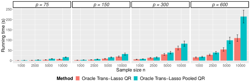
(a)

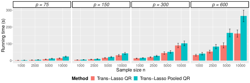
(b)

Figure 11: Average running time comparison for our framework and pooling framework from Huang et al. (2023) under (a) oracle setting and (b) with informative set detection, where the error bar is estimated based on $mean\pm 1.96\times sd$ from 100 repetitions.

Appendix C Features Dictionary of Flight QAR Analysis

Table 1: Feature dictionary for flight QAR data analysis of aggregated measurements.

Code	Definition	Type
3000	Max Airspeed during Flaps Extended	Speed
3001	Max Airspeed during Landing Gear Extended	Speed
3002	Max Airspeed during Speed Brakes Extended	Speed
3005	Average Airspeed during Climb	Speed
3007	Average Airspeed during Cruise	Speed
3009	Average Airspeed during Descent	Speed
3013	Average Airspeed during Engine Stop	Speed
3023	Average Airspeed during PreFlight	Speed
3027	Average Airspeed during Taxi In	Speed
3029	Average Airspeed during Taxi Out	Speed
3035	Max Groundspeed during Turn	Speed
3036	Max Groundspeed during Pre Lift Off	Speed
3037	Max Groundspeed during Straight Line	Speed
3057	Time during Lift Off to Landing Gear Selected Up	Time & Dist
3058	Time during Landing Gear Selected Down to Touchdown	Time & Dist
3070	Time during Climb	Time & Dist
3071	Time during Cruise	Time & Dist
3072	Time during Descent	Time & Dist
3089	Time during Touchdown to Start of All Engine Reverser Deployed	Time & Dist
3090	Time during Final 200 knots CAS to Touchdown	Time & Dist
3093	Max Vertical Acceleration during Flight	Acceleration
3094	Max Vertical Acceleration during Landing	Response
3096	Max Vertical Acceleration during Take Off	Acceleration
3104	Max Vertical Acceleration during Pre Take Off	Acceleration
3105	Max Vertical Acceleration during Post Landing	Acceleration
3112	Average Wind Direction during First 20ft AFE to First 100ft AFE	External
3113	Average Angle of Attack during Cruise	Attitude
3119	Difference in Fuel Consumed Engine 1 during Lift Off to First Cruise	Fuel
3123	Difference in Fuel Consumed Engine 1 during Climb	Fuel
3124	Difference in Fuel Consumed Engine 1 during Cruise	Fuel
3125	Difference in Fuel Consumed Engine 1 during Descent	Fuel
3192	Average Fuel Flow Engine 1 during Climb	Fuel
3193	Average Fuel Flow Engine 1 during Cruise	Fuel
3194	Average Fuel Flow Engine 1 during Descent	Fuel
3195	Average Fuel Flow Engine 1 during Engine Start	Fuel
3201	Average Fuel Flow Engine 1 during PreFlight	Fuel
3203	Average Fuel Flow Engine 1 during Taxi In	Fuel
3204	Average Fuel Flow Engine 1 during Taxi Out	Fuel
3253	Total Ground Distance during Climb	Time & Dist
3254	Total Ground Distance during Cruise	Time & Dist
3255	Total Ground Distance during Descent	Time & Dist
3256	Total Ground Distance during Engine Start	Time & Dist
3265	Total Ground Distance during Taxi Out	Time & Dist
3268	Max Absolute Longitudinal Acceleration during Landing	Acceleration
3271	Average Mach during Climb	Speed
3273	Average Mach during Cruise	Speed
3275	Average Mach during Descent	Speed
3279	Average Mach during Engine Stop	Speed
3293	Average Mach during Taxi In	Speed
3295	Average Mach during Taxi Out	Speed
3344	Max Absolute Bank Angle during Final 50ft AFE to Touchdown	Attitude
3361	Max Airspeed - Take Off Safety Speed during Slats Only Extended	Speed
3362	Max Airspeed - Take Off Safety Speed during Flap Setting 1	Speed
3363	Max Airspeed - Take Off Safety Speed during Flap Setting 2	Speed
3364	Max Airspeed - Take Off Safety Speed during Flap Setting 3	Speed
3365	Max Airspeed - Take Off Safety Speed during Flap Setting 4	Speed
3366	Max Airspeed - Take Off Safety Speed during Flap Setting 5	Speed
3367	Max Airspeed - Take Off Safety Speed during Flap Setting 6	Speed
3368	Max Airspeed - Take Off Safety Speed during Flap Setting 7	Speed
3384	Max Wind Speed during First 20ft AFE to First 100ft AFE	External
3385	Max Absolute Lateral Acceleration during Landing	Acceleration
3387	Min Maximum Operating Speed - Airspeed during Flight	Speed
3418	Max Airspeed - Landing Reference Speed during Slats Only Extended	Speed
3419	Max Airspeed - Landing Reference Speed during Flap Setting 1	Speed
3420	Max Airspeed - Landing Reference Speed during Flap Setting 2	Speed
3421	Max Airspeed - Landing Reference Speed during Flap Setting 3	Speed
3422	Max Airspeed - Landing Reference Speed during Flap Setting 4	Speed
3423	Max Airspeed - Landing Reference Speed during Flap Setting 5	Speed
3424	Max Airspeed - Landing Reference Speed during Flap Setting 6	Speed
3425	Max Airspeed - Landing Reference Speed during Flap Setting 7	Speed
3426	Max Airspeed - Landing Reference Speed during Flap Setting 8	Speed

Table 2: Feature dictionary for flight QAR data analysis of scalar measurements.

Code	Definition	Type
1000	Airspeed at Final Wing Change Configuration before Touchdown	Speed
1001	Airspeed at First Wing Change Configuration after Lift Off	Speed
1002	Airspeed at First Wing Clean Configuration after Lift Off	Speed
1005	Airspeed at Landing Gear Selected Down	Speed
1006	Airspeed at Landing Gear Selected Up	Speed
1018	Altitude at Landing Gear Selected Down	Attitude
1019	Altitude at Landing Gear Selected Up	Attitude
1026	Altitude at Final 200 knots CAS	Attitude
1034	Gross Weight at Start of Flight	Weight
1050	Gross Weight at Start of Taxi Out	Weight
1056	Groundspeed at Start of Off Runway	Speed
1057	Landing Reference Speed at Threshold	Speed
1058	Landing Reference Speed at Touchdown	Speed
1062	Landing Reference Speed at Final 50ft AFE	Attitude
1065	Pitch at Lift Off	Attitude
1070	Pitch Rate at Lift Off	Attitude
1075	Rotation Speed at Rotation	Speed
1076	Take Off Decision Speed, V1 at Lift Off	Speed
1077	Take Off Safety Speed, V2 at Lift Off	Speed
1080	Temperature at Lift Off	External
1081	Temperature at Touchdown	External
1087	Time at Start of Climb	Time & Dist
1088	Time at Start of Cruise	Time & Dist
1096	Time at Start of PreFlight	Time & Dist
1103	Vertical Speed at Touchdown	Speed
1109	Wind Direction at Lift Off	External
1110	Wind Direction at Touchdown	External
1113	Bank Angle at Touchdown	Attitude
1114	Stabilizer Angle at Rotation	Attitude
1115	Wind Speed at Touchdown	External

Appendix D Supplementary Figures of Flight QAR Analysis

References

- Baione and Biancalana (2021) Baione, F. and D. Biancalana (2021). An application of parametric quantile regression to extend the two-stage quantile regression for ratemaking. Scandinavian Actuarial Journal 2021(2), 156–170.
- Bastani (2021) Bastani, H. (2021). Predicting with proxies: Transfer learning in high dimension. Management Science 67(5), 2964–2984.
- Belloni and Chernozhukov (2011) Belloni, A. and V. Chernozhukov (2011). -penalized quantile regression in high-dimensional sparse models. Annals of Statistics 39(1), 82–130.
- Bühlmann and van de Geer (2011) Bühlmann, P. and S. van de Geer (2011). Statistics for High-Dimensional Data. Berlin, Germany: Springer.
- Cai and Guo (2017) Cai, T. T. and Z. Guo (2017). Confidence intervals for high-dimensional linear regression: Minimax rates and adaptivity. The Annals of Statistics 45(2), 615–646.
- Chen and Jin (2021) Chen, R. and J. Jin (2021). Detection of influential features of hard landing based on QAR data. In 2021 IEEE 3rd International Conference on Civil Aviation Safety and Information Technology, pp. 526–529.
- Chen et al. (2020) Chen, X., W. Liu, X. Mao, and Z. Yang (2020). Distributed high-dimensional regression under a quantile loss function. Journal of Machine Learning Research 21(182), 1–43.
- Cheng et al. (2020) Cheng, L., K. Wang, and F. Tsung (2020). A hybrid transfer learning framework for in-plane freeform shape accuracy control in additive manufacturing. IISE Transactions 53(3), 298–312.
- Demir et al. (2022) Demir, A., V. Pesqué-Cela, Y. Altunbas, and V. Murinde (2022). Fintech, financial inclusion and income inequality: a quantile regression approach. The European Journal of Finance 28(1), 86–107.
- Fan et al. (2014) Fan, J., Y. Fan, and E. Barut (2014). Adaptive robust variable selection. Annals of Statistics 42(1), 324.
- Filburn (2020) Filburn, T. (2020). Flight controls, high-lift systems, and their actuation. In Commercial Aviation in the Jet Era and the Systems that Make it Possible, pp. 17–28. Berlin, Germany: Springer.
- Gu et al. (2020) Gu, S., B. Kelly, and D. Xiu (2020). Empirical asset pricing via machine learning. The Review of Financial Studies 33(5), 2223–2273.
- Hong and Jun (2008) Hong, G. and J. Jun (2008). Fuel flow regression model of aircraft cruise based on QAR data. Aeroengine 34(4), 46–50.
- Huang et al. (2023) Huang, J., M. Wang, and Y. Wu (2023). Estimation and inference for transfer learning with high-dimensional quantile regression. arXiv preprint arXiv:2211.14578v3.
- Huang et al. (2017) Huang, Q., H. Zhang, J. Chen, and M. He (2017). Quantile regression models and their applications: A review. Journal of Biometrics & Biostatistics 8(3), 1–6.
- Karbalayghareh et al. (2018) Karbalayghareh, A., X. Qian, and E. R. Dougherty (2018). Optimal bayesian transfer learning. IEEE Transactions on Signal Processing 66(14), 3724–3739.
- Koenker (2005) Koenker, R. (2005). Quantile Regression. New York, United States: Cambridge University Press.
- Koenker and Bassett Jr (1978) Koenker, R. and G. Bassett Jr (1978). Regression quantiles. Econometrica 46(1), 33–50.
- Koenker et al. (2017) Koenker, R., V. Chernozhukov, X. He, and L. Peng (2017). Handbook of Quantile Regression. Florida, United States: CRC Press.
- Koenker and Hallock (2001) Koenker, R. and K. F. Hallock (2001). Quantile regression. Journal of Economic Perspectives 15(4), 143–156.
- Lan et al. (2012) Lan, C. E., W. Kaiyuan, and Y. Jiang (2012). Flight characteristics analysis based on QAR data of a jet transport during landing at a high-altitude airport. Chinese Journal of Aeronautics 25(1), 13–24.
- Li et al. (2021) Li, S., T. T. Cai, and H. Li (2021). Transfer learning for high-dimensional linear regression: Prediction, estimation, and minimax optimality. Journal of the Royal Statistical Society: Series B (Statistical Methodology) 84(1), 149–173.
- Maiti (2021) Maiti, M. (2021). Quantile regression, asset pricing and investment decision. IIMB Management Review 33(1), 28–37.
- Pan and Yang (2009) Pan, S. J. and Q. Yang (2009). A survey on transfer learning. IEEE Transactions on Knowledge and Data Engineering 22(10), 1345–1359.
- Qian et al. (2017) Qian, S., S. Zhou, and W. Chang (2017). An improved aircraft hard landing prediction model based on panel data clustering. In 2017 29th Chinese Control And Decision Conference, pp. 438–443.
- Raskutti et al. (2010) Raskutti, G., M. J. Wainwright, and B. Yu (2010). Restricted eigenvalue properties for correlated gaussian designs. Journal of Machine Learning Research 11, 2241–2259.
- Reich (2012) Reich, B. J. (2012). Spatiotemporal quantile regression for detecting distributional changes in environmental processes. Journal of the Royal Statistical Society: Series C (Applied Statistics) 61(4), 535–553.
- Rigollet and Hütter (2015) Rigollet, P. and J.-C. Hütter (2015). High dimensional statistics. Lecture notes for course 18S997, 46.
- Rogers and Joiner (2018) Rogers, M. L. and T. E. Joiner (2018). Severity of suicidal ideation matters: Reexamining correlates of suicidal ideation using quantile regression. Journal of Clinical Psychology 74(3), 442–452.
- Rosenstein et al. (2005) Rosenstein, M. T., Z. Marx, L. P. Kaelbling, and T. G. Dietterich (2005). To transfer or not to transfer. In NIPS 2005 Workshop on Transfer Learning, Volume 898, pp. 1–4.
- Sun and Xiao (2012) Sun, R. and Y. Xiao (2012). Research on indicating structure for operation characteristic of civil aviation pilots based on QAR data. Journal of Safety Science and Technology 8(11), 49–54.
- Tian and Feng (2023) Tian, Y. and Y. Feng (2023). Transfer learning under high-dimensional generalized linear models. Journal of the American Statistical Association 118(544), 2684–2697.
- Tomczyk (2002) Tomczyk, A. (2002). A proposal of handling qualities shaping for general aviation aircraft. Aircraft Engineering and Aerospace Technology 74(6), 534–549.
- Vershynin (2018) Vershynin, R. (2018). High-dimensional Probability: An Introduction with Applications in Data Science, Volume 47. New York, United States: Cambridge University Press.
- Wainwright (2009) Wainwright, M. J. (2009). Sharp thresholds for high-dimensional and noisy sparsity recovery using -constrained quadratic programming (lasso). IEEE Transactions on Information Theory 55(5), 2183–2202.
- Wang et al. (2014) Wang, L., C. Wu, R. Sun, and Z. Cui (2014). An analysis of hard landing incidents based on flight QAR data. In International Conference on Engineering Psychology and Cognitive Ergonomics, pp. 398–406.
- Wang et al. (2012) Wang, L., Y. Wu, and R. Li (2012). Quantile regression for analyzing heterogeneity in ultra-high dimension. Journal of the American Statistical Association 107(497), 214–222.
- Wei et al. (2006) Wei, Y., A. Pere, R. Koenker, and X. He (2006). Quantile regression methods for reference growth charts. Statistics in Medicine 25(8), 1369–1382.
- Weiss et al. (2016) Weiss, K., T. M. Khoshgoftaar, and D. Wang (2016). A survey of transfer learning. Journal of Big data 3(1), 1–40.
- Xu et al. (2022) Xu, W., S. Chang, Y. Li, R. Doshi, K. Chen, F. Wang, and R. Aseltine (2022). Improving suicide risk prediction via targeted data fusion: proof of concept using medical claims data. Journal of the American Medical Informatics Association 29(3), 500–511.
- Zhao and Yu (2006) Zhao, P. and B. Yu (2006). On model selection consistency of lasso. Journal of Machine Learning Research 7, 2541–2563.
- Zhou (2009) Zhou, S. (2009). Restricted eigenvalue conditions on subgaussian random matrices. arXiv preprint arXiv:0912.4045.
- Zou and Yuan (2008) Zou, H. and M. Yuan (2008). Composite quantile regression and the oracle model selection theory. The Annals of Statistics 36(3), 1108–1126.