“How much do we stand our fellows?
A universal behavior in face-to-face relations”
Supplementary Information

S1 Main results

There are 2 major results in this work.

The first one concerns the duration of face-to-face contacts between each pair of individuals. Although the mean value may vary, the deviation from this mean value is very similar in several very different social contexts. As in other fields of physics (e..g cosmology) we call this over/under-duration the duration contrast. It is a dimensionless value that describes how much given an interaction is longer or shorter than its usual (mean) time and can be expressed in percents. By construction its mean value is 1.

To remove some statistical noise , we only use data where there is a sufficient number of interactions (samples) $N_{int}$. Since the duration distribution is heavy-tailed we use a large minimal value of 50.

Figure 1 (a) shows how the distribution of the duration of contacts and how it changes when computing the contrast in (b). Both use the $N_{int}>50$ cut.

Figure 1: (a) distributions (p.t.e) of the durations of contact and (b) contrast durations on the 4 datasets. The cut $N_{int}>50$ is used for both.

The second major result is the spectacular agreement of our model with the data. We recall how the model proceeds:

1. on a given dataset we loop on all the pair of contacts that were registered (“relation”, $r$) over the full duration of the experiment. We keep only timelines where there are at least 50 intervals of interaction.

2. for a given pair ($r$) we determine its mean duration value : $\bar{t}(r)$.

3. we draw 10 random Levy graph with $\alpha=1.1$ for each relation $r$. Their size is given by the weight $N(r)=w(r)$, and their scale (linking length) by $s(r)=(A\bar{t}(r))^{1/\alpha_{c}}$, where $A\simeq 1$ and $\alpha_{c}\simeq\alpha$ are determined from LGG simulations and are given for some $\alpha$ values in Sect. S5. Times ($w$ and $\bar{t}$) are expressed as a raw number of resolution steps (20 s) and are thus integers.

Although the contrast data are very similar (Figure 1 (b)) we show the results on the 4 datasets since the sizes $N(r)$ and scales $s(r)$ are different in each case.

(a) hosp

(b) conf

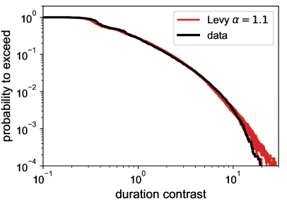
(c) malawi

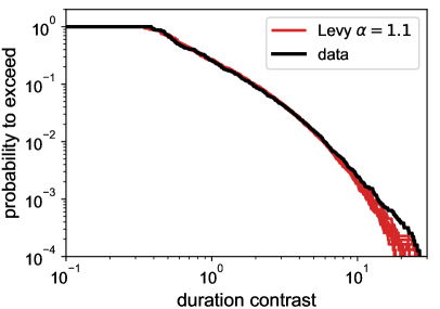
(d) baboons

Figure 2: (a) distributions (p.t.e) of the durations of contact and (b) contrast durations on the 4 datasets. The cut $N_{int}>50$ is used for both.

S2 Other datasets

Although in our work we have focused on the sociologically different datasets, we have also looked at some other data provided by the sociopattern collaboration.

1. conf2: these are data taken at another conference (SFHH,[1, 2]) with $\simeq$380 participants for 2 days.

2. office: data taken at an office (Intitut de Veille Sanitaire near Paris, [3, 4]) with about 165 participants for 10 days.

3. highschool: data from a french high-school, near Marseille [5, 6]. About 300 participants for 4 days

As in Sect. S1 we show how using the contrast standardizes the contact durations on Figure 3 on these new datasets; for comparison we also included the previous conf result and still use the $N_{int}>50$ cut.

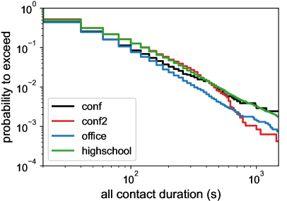
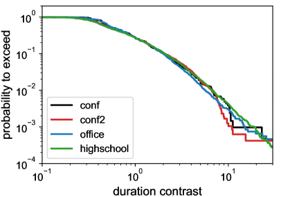
Figure 3: (a) distributions (p.t.e) of the durations of contact and (b) contrast durations for 3 other datasets.

The contrast distributions are similar to the results presented in the paper, and differences are barely noticeable in a linear representation.

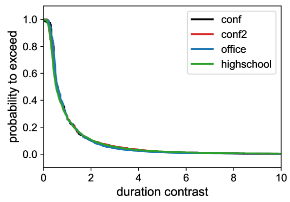
Figure 4: Same as Figure 3 (b) in linear scale.

S3 Number of interactions

To compute a mean value one (traditionally) invokes the central limit theorem and compute a reliable arithmetic mean with $\simeq 20$ samples . However the contact duration distribution is very wide (Figure 1(a)) so we prefer to increase that value to $N_{int}>50$ before computing the contrast, still keeping a reasonable number of timelines in each case. We may use a lower cutoff and the contrasts distributions are still similar(Figure 5) . But we have added some noisy samples. Note that this value of 50 is only dictated by the data limit data-taking period. Had we a really long period, the mean interaction times between each pair would be well known and this cut would be not necessary.

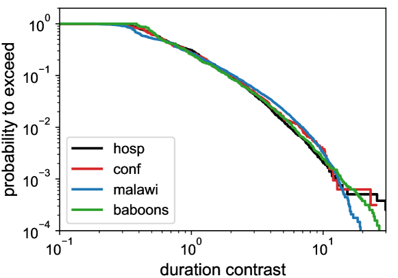
Figure 5: Distribution of the contrast durations on the 4 datasets using a $N_{int}(r)>30$ cut.

S4 Simulations without a minimal number of interactions

S4.1 Combined contrast

We have shown in the manuscript how to reproduce the noise present on the data for all $N_{int}$ values on the conf dataset in Section 3. Figure 6 shows the results for the other datasets. We reproduce all the data, using only a small fraction of the timelines (the ones with $N_{int}>50$ which represents respectively ).

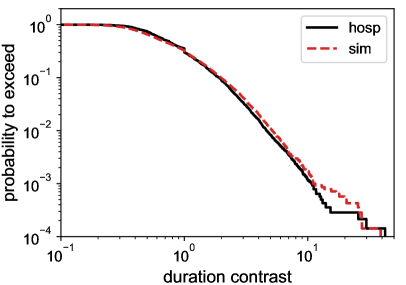
(a) hosp

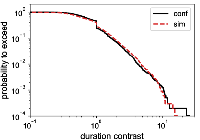
(b) conf

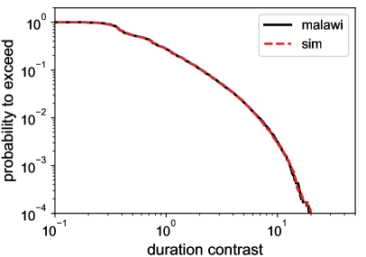
(c) malawi

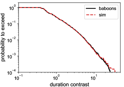
(d) baboons

Figure 6: Results of the simulations described in the manuscript (Sect 3) without using a cut on $N_{int}$ for all the datasets.

S4.2 Contrast per relation

In the previous section, the duration (and contrast) of all contacts are combined on Figure 6 in the sense the contrast of each relation are mixed together. We now consider each relation and show its contrast p.t.e with different colors. The timelines are noisy since we do not use any minimal number of steps ($N_{int}$). The baboons result is less noisy but this is only due to the fact that the timelines have more samples due to the longer data-taking period (26 days).

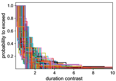
(a) hosp

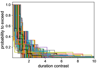
(b) conf

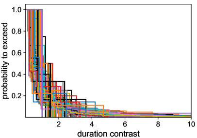
(c) malawi

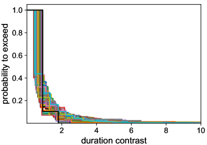
(d) baboons

Figure 7: Contrast distributions per relation measured on the data without any $N_{int}$ cut. Each color represents a different relation timeline.

We then perform the same simulations than described in the manuscript, but this time on each relation individually. Once again only the global shape of the contrast obtained with the $N_{int}>50$ cut (i.e. Figure 1(b)) is used to draw the random numbers. The results are shown on Figure 8. They resembles closely the data (Figure 7). This confirms that the shape and spread observed on data (Figure 7) can be reproduced using only the cleaned Figure 1 distribution ($N_{int}(r)>50$ and statistical fluctuations (on the mean) due to the limited size statistics.

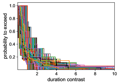
(a) hosp

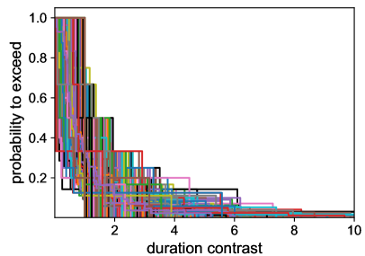
(b) conf

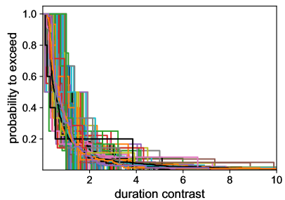
(c) malawi

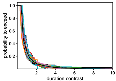
(d) baboons

Figure 8: Results of the simulations described in the manuscript (Sect 3) for each relation (colored curves) without using a cut on $N_{int}$ for all the datasets.

S5 Number of clusters in Levy graphs

As shown in [7], the mean fraction of clusters follows a power-law function of the scale with a relatively small spread among realizations

$$\dfrac{N_{clus}}{N}=\dfrac{A}{s^{\alpha_{c}}}$$ (1)

$A$ and $\alpha_{c}$ are determined using 1000 realizations of LGGs for a fixed $\alpha$ value and varying the scale $s$ between 1 and 10. Figure 9 shows the results and the power-law fits. The resulting parameters are given in Table 1

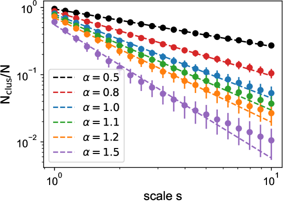
Figure 9: Mean fraction of clusters as a function of the scale as determined from LGG simulations for several $\alpha$ values. Dashed lines represent the best power-law fits.

$\alpha$	A	$\alpha_{c}$
0.50	$0.95\pm 0.01$	$0.56\pm 0.01$
0.80	$0.87\pm 0.02$	$0.95\pm 0.02$
1.00	$0.79\pm 0.02$	$1.25\pm 0.04$
1.10	$0.75\pm 0.02$	$1.40\pm 0.05$
1.20	$0.70\pm 0.03$	$1.55\pm 0.06$
1.50	$0.55\pm 0.03$	$1.98\pm 0.09$

Table 1: Coefficients of eq. 1 fitted from the 2D LGG simulations (Figure 9) for various $\alpha$ values.

S6 Poisson duration

Dividing my mean-values does not necessarily lead to distributions of the Figure 1 kind. We illustrate that feature by computing the contrast using Poisson-distributed durations. To this purpose we use the hosp data to obtain the $\bar{t}(r)$ values for each relation; we then draw $N_{int}(r)$ random numbers following a Poisson distribution of parameter $\bar{t}(r)$, determine the arithmetic mean and compute the contrast. The result is show on Figure 10 which is clearly different from the results observed on data.

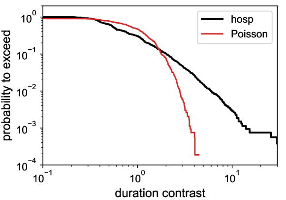
Figure 10: Distribution of the contrast durations assuming Poisson distributed durations. The parameters are taken from the hosp dataset and the data result is recalled in red.

S7 Dimension above 2

A Levy flight can be generalized to any dimension (see [7] for a simple algorithm). For our model, we have tried several dimension. Figure 11 shows the result in dimension 3 (note that the coefficients $A$ and $\alpha_{c}$ from Sect. S5 have been recomputed). Compared to dimension 2 (see Figure 2 (c)), the agreement with the malawi data gets worse. If we further increase the dimension the return probability of the walk decreases and the contrast goes to $\exp(-\delta)$ which is clearly far from the data.

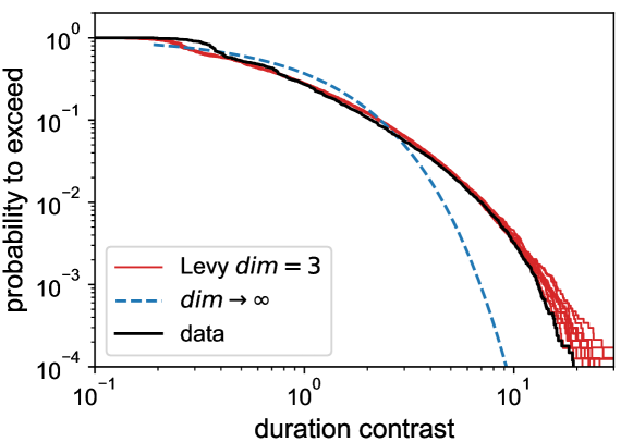
Figure 11: Levy model ($\alpha=1.1$) in red compared to the malawi data (in black) for a Levy walk in a space of dimension 3. Increasing the dimension further, the model converges to the dashed blue line.

S8 Effect of the time resolution

The timing resolution of the experiments affects our model in two ways. The size and scale of each LGG (thus relation) are given by

$$N(r) =\sum_{i=1}^{N_{int}(r)}t_{i}(r)$$ (2)

$$s(r) =\left[A\bar{t}(r)\right]^{1/\alpha_{c}}$$ (3)

where $A\simeq 1,\alpha_{c}\simeq\alpha$ (see Sect. S5).

$t_{i}$ and $\bar{t}$ are expressed as a number of resolution steps (which in the paper is $T=20$ s). We may artificially change it, assuming for instance a resolution of $T=5$ s, in which case we multiply the $t_{i}$’s and $\bar{t}$ by a factor 4. This changes for each graph the values of $N$ and $s$. The result on the contrast distribution for this model are shown on Figure 12.

Compared to Figure 2(c) this model fits less well the data which is normal since we have used a fake resolution. It shows that the wiggles at the beginning of the distribution are due to the $T=20$ s resolution. A prediction from our model is thus that the contrast distribution should be smoother and slightly different if we have data with a better timing resolution.

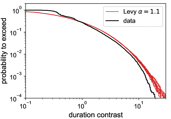
Figure 12: Levy model ($\alpha=1.1$) modified by increasing the resolution to T=5 s (red curves) compared to the malawi dataset.

References

- [1] Ciro Cattuto, Wouter Van den Broeck, Alain Barrat, Vittoria Colizza, Jean-François Pinton, and Alessandro Vespignani. Dynamics of Person-to-Person Interactions from Distributed RFID Sensor Networks. PLoS ONE, 5(7):e11596, July 2010.
- [2] Juliette Stehlé, Nicolas Voirin, Alain Barrat, Ciro Cattuto, Vittoria Colizza, Lorenzo Isella, Corinne Régis, Jean-François Pinton, Nagham Khanafer, Wouter Van den Broeck, and Philippe Vanhems. Simulation of an SEIR infectious disease model on the dynamic contact network of conference attendees. BMC Medicine, 9(1):87, December 2011.
- [3] Mathieu Génois, Christian L. Vestergaard, Julie Fournet, André Panisson, Isabelle Bonmarin, and Alain Barrat. Data on face-to-face contacts in an office building suggest a low-cost vaccination strategy based on community linkers. Network Science, 3(3):326–347, September 2015.
- [4] Mathieu Génois and Alain Barrat. Can co-location be used as a proxy for face-to-face contacts? EPJ Data Science, 7(1):11, May 2018.
- [5] Julie Fournet and Alain Barrat. Contact Patterns among High School Students. PLoS ONE, 9(9):e107878, September 2014.
- [6] Rossana Mastrandrea, Julie Fournet, and Alain Barrat. Contact patterns in a high school: A comparison between data collected using wearable sensors, contact diaries and friendship surveys. PLoS ONE, 10(9):e0136497, 09 2015.
- [7] S. Plaszczynski, G. Nakamura, C. Deroulers, B. Grammaticos, and M. Badoual. Levy geometric graphs. Phys. Rev. E, 105:054151, May 2022.