Hierarchies in relative Picard-Lefschetz theory

Abstract.

We prove a relative version of the Picard-Lefschetz theorem, describing the variation of relative homology groups $H_{d}(Y_{t}\setminus A_{t},B_{t}\setminus A_{t})$ in the fibers of a smooth fiber bundle $Y\to T$ of complex manifolds with $A\cup B\subset Y$ transverse. From this we derive the vanishing of certain iterated variations, a system of constraints dubbed “hierarchy”.

As applications, we rederive the known analytic structure of Aomoto polylogarithms and massive one loop Feynman integrals. Moreover, we introduce the “simple type” to prove hierarchy constraints in degenerate cases where the Picard-Lefschetz formula does not apply, e.g. the massless triangle or the ice cream cone Feynman diagram. We compare our findings with a “classical” hierarchy of iterated variations (from 1960’s $S$-matrix theory) and show how our setup not only explains, but also refines the latter. In order to do so, we need to further resolve the geometry of Feynman motives: We boldly blow up what no one has blown up before.

1. Introduction

1.1. Monodromy

A holomorphic surjection $\pi\colon Y\rightarrow T$ of connected complex manifolds defines a family $Y_{t}=\pi^{-1}(t)$ of analytic varieties that depend on a parameter $t\in T$. The set $L\subset T$ of critical values has measure zero, and the smooth fibres $Y_{t}$ over the complement of $L$ glue into a smooth fibre bundle if $\pi$ is proper. Such local trivializations $\pi^{-1}(U)\cong Y_{t_{0}}\times U$ over $t_{0}\in U\subseteq T\setminus L$ show that the homology groups $H_{d}(Y_{t};\mathbb{Z})$ of the fibres are locally constant over $T\setminus L$. The monodromy representation

$$\pi_{1}(T\setminus L,t_{0})\longrightarrow\operatorname{Aut}H_{d}(Y_{t_{0}};\mathbb{Z})$$

is induced by parallel transport along paths. It is an important tool to study periods of algebraic varieties and variations of Hodge structures [26].

More generally, two analytic subvarieties $A,B\subset Y$ give rise to a family of pairs $B_{t}\setminus A_{t}\subset Y_{t}\setminus A_{t}$ where $A_{t}=A\cap Y_{t}$ and $B_{t}=B\cap Y_{t}$. We abbreviate the associated relative homology groups as

$$H_{d}(Y\setminus A,B)_{t}=H_{d}(Y_{t}\setminus A_{t},B_{t}\setminus A_{t};\mathbb{Z}).$$

To describe their monodromy, we seek:

1. a subset $L\subset T$ such that the pairs $(Y_{t}\setminus A_{t},B_{t}\setminus A_{t})$ vary as a pair of topological fibre bundles over $T\setminus L$, and

2. the representation $\rho\colon\pi_{1}(T\setminus L,t_{0})\longrightarrow\operatorname{Aut}H_{d}(Y\setminus A,B)_{t_{0}}$.

The Landau variety of the pair $(Y\setminus A,B\setminus A)$ with respect to $\pi$ is a closed analytic subvariety $L$ of $T$ with property (L). We will describe the monodromy $\gamma_{*}=\rho(\gamma)$ along a loop $\gamma\in\pi_{1}(T\setminus L,t_{0})$ in terms of the variation

$$\operatorname{Var}_{\gamma}=\gamma_{*}-\operatorname{id}\in\operatorname{End}H_{d}(Y\setminus A,B)_{t_{0}}.$$

1.2. Parameter integrals

The monodromy data encodes the analytic continuation (V), and a bound (L) on the singularities, of parameter integrals

$$\mathcal{I}(t)=\int_{\sigma_{t}}\omega_{t}$$

of integrands with poles on $A$, over domains with boundary in $B$. Let

• $n$ the complex dimension of the fibres $Y_{t}$,

• $\omega\in\Omega^{n}(Y\setminus A)$ a holomorphic differential form,

• $\omega_{t}=\omega|_{Y_{t}\setminus A_{t}}$ its restriction to a fibre,

• $\sigma_{t_{0}}$ an $n$-chain in $Y_{t_{0}}\setminus A_{t_{0}}$ with boundary in $B_{t_{0}}\setminus A_{t_{0}}$.

The class $[\sigma_{t_{0}}]$ extends to a multivalued section $[\sigma_{t}]\in H_{n}(Y\setminus A,B)_{t}$ over $T\setminus L$, representable locally by a continuous family $\sigma_{t}$ of chains. Since $\omega_{t}$ is smooth on the compact support of $\sigma_{t}$, the integrals $\mathcal{I}(t)$ converge and define a multivalued holomorphic function on $T\setminus L$. As restrictions of a global form $\omega$, the integrands $\omega_{t}$ are single-valued. Analytic continuation $\gamma\cdot\mathcal{I}$ along a loop $\gamma\in\pi_{1}(T\setminus L,t)$ is thus completely determined by the monodromy:

$$\gamma\cdot\mathcal{I}(t)=\int_{\gamma_{*}[\sigma_{t}]}\omega_{t}=\mathcal{I}(t)+\int_{\operatorname{Var}_{\gamma}[\sigma_{t}]}\omega_{t}.$$

By Riemann’s extension theorem, $\omega$ extends holomorphically over any irreducible components of $A$ with complex codimension $\geq 2$. We hence drop all such components and assume that $A$ is pure of codimension one. Locally,

$$\omega=\sum_{i_{1}<\cdots<i_{n}}\frac{P_{i_{1}\!\cdots i_{n}}(z)}{Q(z)}\ \mathrm{d}z_{i_{1}}\wedge\ldots\wedge\mathrm{d}z_{i_{n}}$$

can be written with holomorphic functions $P$ and $Q$ such that $A$ is the vanishing locus $\{Q=0\}$ of the denominator.

Similarly, the singularities of $\mathcal{I}$ are covered already by only those components $\ell_{i}\subseteq L$ with complex codimension one. Items (L) and (V) above translate into finding an upper bound $L$ on the singularities $\bigcup_{i}\ell_{i}$ of $\mathcal{I}$, and studying the behaviour of $\mathcal{I}$ near each $\ell_{i}$. This purely homological approach is blind to the specific choice of the integrand $\omega$, and some integrands produce integrals with fewer singularities (consider e.g. $\omega=0$). We are not concerned with identifying precisely which components $\ell_{i}\subseteq L$ of the Landau variety are genuine singularities of the integral $\mathcal{I}$ for a given $\omega$—instead, the homological approach provides insights that hold for all integrands.

1.3. Picard-Lefschetz theory

Let

$$\mathfrak{A}=\{A_{1},A_{2},\ldots\}\quad\text{and}\quad\mathfrak{B}=\{B_{1},B_{2},\ldots\}$$

denote the finite sets of irreducible components of $A$ and $B$. We assume that these are smooth hypersurfaces with transverse intersections. Suppose that $\ell\subseteq L$ is a component such that $A\cup B$ has a unique, non-degenerate critical point $p(t)$ over $t\in\ell$. Let $A_{1},\ldots,A_{i},B_{1},\ldots,B_{j}$ denote the hypersurfaces that contain $p(t)$. Then for a small loop $\gamma$ in $T\setminus L$, that is based at $t_{0}$ and winds around $\ell$, the Picard-Lefschetz formula

(1.1) $$\operatorname{Var}_{\gamma}(\sigma)=(-1)^{(n+1)(n+2)/2}\cdot\langle{\widetilde{\nu}_{p}}\,|\,{\sigma}\rangle\cdot\nu_{p}$$

determines the variation of $\sigma\in H_{n}(Y\setminus A,B)_{t_{0}}$ in terms of an intersection number $\langle{\widetilde{\nu}_{p}}\,|\,{\sigma}\rangle$ and vanishing cycles $\nu_{p}\in H_{n}(Y\setminus A,B)_{t_{0}}$, $\widetilde{\nu}_{p}\in H_{n}(Y\setminus B,A)_{t_{0}}$. The latter are constructed out of a sphere $\mathbb{S}^{n-i-j}$ localized near $p(t)$ and embedded in the submanifold $A_{1}\cap\ldots\cap A_{i}\cap B_{1}\cap\ldots\cap B_{j}$.

For a single hypersurface $\lvert\mathfrak{A}\sqcup\mathfrak{B}\rvert\leq 1$, the Picard-Lefschetz theorem is well-known [60, 61]. A proof, allowing for arbitrary isolated critical points, can be found in [34, §5]. There are even generalizations for isolated critical points on complete intersections [28, 40]. However, the case with multiple hypersurfaces has not been studied as much. Arrangements with $\lvert\mathfrak{A}\rvert>1$ are treated in [21], but without boundary ($B=\varnothing$). The generalization to $B\neq\varnothing$ is briefly mentioned in [51], but important details are left out.

The first result of this paper is a detailed, self-contained proof of (1.1) in the general case where $A,B\neq\varnothing$. The main new insights are:

• We correct an error in the literature: All sources claim that all linear pinches ($i+j=n+1$) have zero variation. As section 1.8.1 shows, this is not the case. Only the linear pinches of “pure $\mathfrak{A}$ type” ($j=0$) or “pure $\mathfrak{B}$ type” ($i=0$) have zero variation, whereas linear pinches on mixed intersections of $\mathfrak{A}$’s and $\mathfrak{B}$’s have non-zero variation.

• We prove a fairly general vanishing statement for iterated variations, see section 1.4.

The main point of this paper is therefore that it pays off to keep track of which elements of $\mathfrak{A}$ and $\mathfrak{B}$ contain a given critical point. The distinction between $\mathfrak{A}$ and $\mathfrak{B}$ is important, despite the fact that the Landau variety $L$ depends only on the combined arrangement $A\cup B$.

1.4. Hierarchy principle

Consider an iterated variation around two components $\ell,\ell^{\prime}$ of the Landau variety. The hierarchy principle is a combinatorial criterion that ensures $\operatorname{Var}_{\gamma^{\prime}}\circ\operatorname{Var}_{\gamma}=0$. Suppose for example that the fibres over $\ell$ and $\ell^{\prime}$ have a single non-degenerate critical point $p$ and $p^{\prime}$, respectively. Then according to (1.1), we are asking if $\langle{\widetilde{\nu}_{p^{\prime}}}\,|\,{\nu_{p}}\rangle=0$.

The set of all hypersurfaces in $\mathfrak{A}\sqcup\mathfrak{B}$ that contain $p$ encodes a pair

$$(I,J)=(\{i\colon p\in A_{i}\},\{j\colon p\in B_{j}\}),$$

called the type of $p$. Let $(I^{\prime},J^{\prime})$ denote the type of $p^{\prime}$. The variation around $\ell$ localizes in a small neighbourhood of $p$, which meets only those $A_{i}$ and $B_{j}$ with $i\in I,j\in J$. Hence the vanishing cycle $\nu_{p}$ is in the image of

$$H_{n}\Big{(}Y\setminus A,\bigcup\nolimits_{j\in J}B_{j}\Big{)}_{t_{0}}\longrightarrow H_{n}(Y\setminus A,B)_{t_{0}},$$

and therefore the boundary of $\nu_{p}$ remains forever confined to the $B_{j}$ with $j\in J$—even after continuation from $t_{0}$ to any $t\in T\setminus L$.

Furthermore, $\nu_{p}$ is an iterated Leray coboundary (tube) around each $A_{i}$ with $i\in I$. It follows that for any $i\in I$, $\nu_{p}$ is in the kernel of

$$H_{n}(Y\setminus A,B)_{t_{0}}\longrightarrow H_{n}\Big{(}Y\setminus\bigcup\nolimits_{k\neq i}A_{k},B\Big{)}_{t_{0}}.$$

So if some $i\in I$ is not in $I^{\prime}$, then $\nu_{p}$ becomes zero in the localization of $\operatorname{Var}_{\gamma^{\prime}}$ near $p^{\prime}$. A dual argument for the vanishing cycles $\widetilde{\nu}_{p^{\prime}}$ shows that $\langle{\widetilde{\nu}_{p^{\prime}}}\,|\,{\nu_{p}}\rangle=0$ holds also whenever there exists $j\in J^{\prime}$ that is not in $J$.

To summarize, the iterated variation $\operatorname{Var}_{\gamma^{\prime}}\circ\operatorname{Var}_{\gamma}$ can only be nonzero if $p$ and $p^{\prime}$ are compatible (denoted $p^{\prime}\leqslant p$), that is, if

(1.2) $$I^{\prime}\supseteq I\quad\text{and}\quad J^{\prime}\subseteq J.$$

Therefore, a non-zero iteration of variations $\operatorname{Var}_{n}\circ\cdots\circ\operatorname{Var}_{1}$ requires that the sets of participating $\mathfrak{B}$-elements get smaller ($I_{1}\supseteq I_{2}\supseteq\ldots$), whereas the sets of $\mathfrak{A}$-elements can only get bigger ($J_{1}\subseteq J_{2}\subseteq\ldots$).

In section 4 we generalize this property in various ways:

• For linear simple pinches (3.13), compatibility requires strict containment: $I^{\prime}\supsetneq I$ and $J^{\prime}\subsetneq J$.

• When there are multiple critical points in a fiber, we call two components of the Landau variety compatible ($\ell^{\prime}\leqslant\ell$), if all critical points over $\ell^{\prime}$ are compatible with all critical points over $\ell$.

• We can allow critical points that are not simple pinches, or critical sets $p\subset A^{I}\cap B^{J}$ that are not even isolated. Then (1.2) becomes

  (1.3) $$I^{\prime}\supseteq I_{\mathsf{s}}\quad\text{and}\quad J_{\mathsf{s}}^{\prime}\subseteq J,$$

  in terms of the simple components $I_{\mathsf{s}}\subseteq I$ and $J_{\mathsf{s}}^{\prime}\subseteq J$ (4.9). Here a component $A_{i}$ or $B_{j}$ is called simple, if $p$ remains critical even if that component is removed from the arrangement.

The upshot is a relation $\leqslant$ on the components $\ell$ of $L$ (4.17). The hierarchy principle (4.18) states then that

(1.4) $$\operatorname{Var}_{\gamma^{\prime}}\circ\operatorname{Var}_{\gamma}=0\quad\text{if}\quad\ell^{\prime}\nleqslant\ell.$$

As an application, we show in sections 5.1 and 6.1 how to quickly derive the known Landau variety and hierarchy for Aomoto polylogarithms and massive one loop Feynman integrals.

1.5. Feynman integrals

The application of homological methods to Feynman integrals has a long history [31, 23]. Approaches using the momentum representation, like [20, 63], are complicated by the need to compactify the integration domain, which poses unsolved challenges beyond one loop [46].

This problem does not appear in the parametric representation. However, in this representation, the integration domain has boundary. An analysis of (iterated) variations therefore requires a relative version of the (hierarchy) Picard-Lefschetz theorems. Using this setup, Boyling derived constraints of the form (1.4) for massive one-loop graphs [10, §2].

The Picard-Lefschetz formula (1.1) is however not usually applicable to more general Feynman integrals, because the critical sets are often not simple and isolated. Using our generalized hierarchy principle, we can nevertheless obtain constraints on iterated variations in such cases. We carry this out in detail for Feynman graphs with two loops (sunrise and ice cream cone) or one loop and zero masses (triangle), see section 6.

We find that the distinction in (1.3) between the type of a singularity $\ell\subset L$ vs. its simple components is indeed crucial: applying (1.2) to singularities that are not simple pinches leads to wrong conclusions. This need for a refined analysis was noted for Feynman integrals in [36], correcting a too optimistic expectation for the $\mathfrak{B}$-hierarchy from [37]. In sections 6.1 and 6.4 we demonstrate that also the $\mathfrak{A}$-hierarchy is interesting for Feynman integrals.

1.6. Outlook

The techniques developed in this paper provide a framework to explain variation constraints of the form (1.4). We hope that these methods will be useful to prove constraints for infinite families of Feynman integrals, and thereby scattering amplitudes. For example, extended Steinmann relations [15, §3] are applied with great effect in high order perturbation theory. For now, these relations and generalizations thereof [18] are conjectures.

Remark 1.1.

Originally, Steinmann relations [38, 55] refer to amplitudes—not individual Feynman diagrams—and they only apply in a restricted (“physical”) region of parameter space. This translates into the statement $\operatorname{Var}_{\gamma^{\prime}}\operatorname{Var}_{\gamma}\sigma=0$ for certain chains $\sigma$, but not all. In the physical region, first type singularities have simple pinch type and can thus be studied with Picard-Lefschetz theory [49, 50, 29]. The resulting hierarchy has a simple formulation, but it does not apply outside the physical region, ignores singularities of second type, and requires generic masses.

We do not make any such assumptions.

1.7. Outline of the paper

In section 2 we review the solution of problem (L), that is, how to find the Landau variety of a pair $(Y\setminus A,B\setminus A)$ with respect to a smooth map of complex manifolds $\pi\colon Y\to T$. We discuss (canonical) stratifications, Thom’s first isotopy lemma (including a smooth version of it), how to compute $L$ and how this applies to the study of parameter integrals.

Section 3 deals then with problem (V) via Picard-Lefschetz theory. We review the classical Picard-Lefschetz theorem and prove its generalization to relative homology. In the process, we give a concise account of all necessary technical tools: Definition of the monodromy and variation operators, localization arguments, characterization of simple pinch critical points, Leray’s residue and (co)boundary maps, and definition of the vanishing chains. After the stage is set, we state and prove the (relative) Picard-Lefschetz theorem, 3.21, then discuss refinements for linear pinches (3.22) and generalizations to arbitrary simple pinches (eq. 3.22).

In section 4 we introduce our hierarchy principle. We first present it for simple pinches (eqs. 4.3, 4.4, 4.5 and 4.6), then for certain components of the Landau variety (4.7), and finally state it in its most general form (corollaries 4.16 and 4.18) which allows for non-isolated critical sets.

The following two sections apply the previously developed theory to two families of examples. We rigorously derive their Landau varieties and discuss implications (and limitations) of the hierarchy principle. In section 5 we consider polylogarithms: While section 5.2 deals with a specific (slightly degenerate) example, the dilogarithm, section 5.1 discusses a tame family, the Aomoto polylogarithms, in full detail. Finally, in section 6 we study Feynman integrals. After introducing some notation, we start with massive one loop graphs (section 6.1) where our setup works out of the box. Then we consider some specific examples where this is not the case, the massless triangle, the massive sunrise and the ice cream cone. We show how additional blow ups (beyond the Feynman motive) turn $A\cup B$ transverse, so that we can apply our methods. This allows us to explain and refine what is called breakdown of the hierarchical principle in [10, 36].

The appendices provide several technical details, that are hard to find in the existing literature:

• Appendix A calculates all relative homology groups of the arrangement of hypersurfaces at a linear or quadratic simple pinch, generalizing results of [21]. To be fully self-contained, we also compute the classical Picard-Lefschetz formula for the variation of a quadric.

• Appendix B explains the construction of the long exact sequences for partial boundaries and relative residues from [39, Chapitre 2], in the general case of transverse arrangements of smooth closed submanifolds with arbitrary codimensions.

• Appendix C gives a general definition and the key properties of relative intersection numbers and the duality swapping $A\leftrightarrow B$.

• Appendix D shows that the codimension one components $\ell$ of $L$ already determine the full fundamental group $\pi_{1}(T\setminus L)$, and that the kernel of $\pi_{1}(T\setminus L)\relbar\joinrel\twoheadrightarrow\pi_{1}(T)$ is generated by so-called simple loops (3.1).

1.8. Two examples

We illustrate our findings with two very simple examples: The first example observes that the non-trivial monodromy of the logarithm arises from a linear pinch; the second example illustrates the hierarchy principle for the bubble Feynman integral. In both cases, $Y=X\times T$ is a product with $\pi(x,t)=t$ and compact fibre $X=\mathbb{P}^{1}$.

1.8.1. The logarithm

For $t\in\mathbb{P}^{1}$ consider the integral

$$\log(1-t)=\int_{\sigma}\frac{t\,\mathrm{d}x}{tx-1}.$$

For $t\neq[1,\infty]$, the interval $\sigma=[0,1]$ defines a class in $H_{1}(X\setminus A_{t},B_{t})$, where the hypersurfaces $\mathfrak{A}=\{A_{1},A_{2}\}$ and $\mathfrak{B}=\{B_{1},B_{2}\}$ of $Y$ are given by

$$A_{1}=\{xt=1\},\ A_{2}=\{x=\infty\},\ B_{1}=\{x=0\},\ B_{2}=\{x=1\}.$$

These four hypersurfaces are smooth and transverse to each other. Each hypersurface submerses onto $T$. Thus, the critical strata are the points (codimension two) where two hypersurfaces in $\mathfrak{A}$, or one in $\mathfrak{A}$ and one from $\mathfrak{B}$, intersect (see fig. 1):

$$\begin{cases}\{xt=1\}\cap\{x=\infty\}=\{(\infty,0)\},&\mathfrak{A}\cap\mathfrak{A}\\ \{xt=1\}\cap\{x=0\}=\{(0,\infty)\},&\mathfrak{A}\cap\mathfrak{B}\\ \{xt=1\}\cap\{x=1\}=\{(1,1)\},&\mathfrak{A}\cap\mathfrak{B}.\\ \end{cases}$$

Figure 1. The arrangement $D=A\cup B\subset\mathbb{P}^{1}\times\mathbb{P}^{1}$ associated to the integral $\log(1-t)=\int_{\sigma_{t}}\frac{t\,\mathrm{d}x}{tx-1}$.

These critical points are called linear pinches and their projection along $\pi$ determines the Landau variety $L=\{0,1,\infty\}$. At the points $t=1,\infty$, the function $\log(1-t)$ has logarithmic singularities. In contrast, at $t=0$, this function is smooth and takes values in $2\mathrm{i}\pi\mathbb{Z}$. In particular, the variation at $t=0$ is zero. We will see in general that linear pinches of “pure $\mathfrak{A}$-type” (or “pure $\mathfrak{B}$-type”) always have zero variation, whereas “mixed $\mathfrak{A}$–$\mathfrak{B}$-type” linear pinches have non-zero variation.

In order to describe the monodromy associated to small loops winding around $L$ we note that for generic $t$ the first relative Betti homology of the fiber is $H_{1}(Y\setminus A,B)_{t}=H_{1}(X\setminus A_{t},B_{t})\cong\mathbb{Z}^{2}$. It is spanned by the interval $\sigma=[0,1]$, and a small loop $\nu$ around the point $x={t}^{-1}$. This cycle is constructed as follows (see fig. 2):

1. Let $\ell\in L$. For $t$ close to $\ell$ we consider the pair of fibers $(X,A_{t}\cup B_{t})$. The vanishing cell $\zeta_{\ell}$ is the unique (real) $n$-dimensional cell ($n=\dim_{\mathbb{C}}X$) in $X$ that is bounded by $A_{t}\cup B_{t}$ and vanishes as $t\to\ell$.

   In the present case there are three such cells, given by paths from $x$ to ${t}^{-1}$ for $x=0,1,\infty\in X$ (corresponding to $\ell=\infty,1,0$). Each represents an element in $H_{1}(Y,A\cup B)_{t}\cong\mathbb{Z}^{3}$. Note that, if we restrict to a small neighbourhood $U$ of a critical point $x={\ell}^{-1}$, then each class is the unique generator of $H_{1}(U,(A_{t}\cup B_{t})\cap U)\cong\mathbb{Z}$.

2. The vanishing cycle $\nu_{\ell}$ is defined as the Leray coboundary (see section 3.4) of the partial boundary of the vanishing cell (both with respect to the relevant hypersurfaces of $\mathfrak{A}$-type), $\nu_{\ell}:=\delta_{A}\partial_{A}\zeta_{\ell}$.

   Here $\nu_{1}$ and $\nu_{\infty}$ coincide, both given by small loops around $x={t}^{-1}$. They represent classes $[\nu_{1}]\equiv[\nu_{\infty}]$ in $H_{1}(Y\setminus A,B)_{t}$, unique after localisation. The vanishing cycle $\nu_{0}$ is zero, because $\partial_{A}\zeta_{0}=\partial_{A_{2}}\partial_{A_{1}}\zeta_{0}=0$.

Figure 2. Geometry of $\log(1-t)$: The left hand side shows the vanishing cell $\zeta_{1}$ and vanishing cycle $\nu_{1}$ for $t$ close to 1, the right hand side sketches the monodromy of $\sigma$ associated to a small loop winding around $t=1$; the resulting relative cycle $\widetilde{\sigma}$ is homologous to $\sigma+\nu_{1}$.

The Picard-Lefschetz theorem states that the variation $\operatorname{Var}_{\ell}$ associated to a small loop winding around $\ell$ maps a homology class $h\in H_{n}(Y\setminus A,B)_{t}$ to a multiple of the vanishing cycle $N[\nu_{\ell}]$ where $N\in\mathbb{Z}$ is determined by a (relative) intersection index $\langle{\partial_{B}h}\,|\,{\partial_{B}\zeta_{\ell}}\rangle$ with $\partial_{B}$ denoting the iterated partial boundary with respect to $B$.

In the present case we have $\nu_{0}=0$, so the variation associated to $0\in L$ vanishes. For $\ell=1,\infty$ one calculates $\langle{\partial_{B}\sigma}\,|\,{\partial_{B}\zeta_{\ell}}\rangle=\pm 1$, while $\langle{\partial_{B}\nu_{\ell}}\,|\,{\partial_{B}\zeta_{\ell}}\rangle=\langle{0}\,|\,{\partial_{B}\zeta_{\ell}}\rangle=0$. In summary, the variation of $[\sigma]$ is non-trivial around $\ell=1,\infty$, the variation of $[\nu_{1}]=[\nu_{\infty}]$ is trivial around all points of $L$. We recover thus the well-known analytic structure of the function $\log(1-t)$.

1.8.2. The bubble Feynman integral

As a second example we consider the parametric Feynman integrals (cf. section 6) of the bubble graph:

$$\mathcal{I}(p^{2},m_{1}^{2},m_{2}^{2})=\int_{\sigma=\{[x_{1}:x_{2}]\colon x_{i}>0\}}\frac{P\Omega}{\mathcal{U}^{a}\mathcal{F}^{b}}=\int_{0}^{\infty}\left.\frac{P}{\mathcal{U}\mathcal{F}}\right|_{x_{1}=1}\mathrm{d}x_{2}.$$

Here $a$ and $b$ are integers, $P$ is any homogeneous polynomial in $x$ with degree $a+2b-2\geq 0$, the projectivized measure is $\Omega=x_{1}\mathrm{d}x_{2}-x_{2}\mathrm{d}x_{1}$, and

$$\mathcal{U}=x_{1}+x_{2},\qquad\mathcal{F}=(x_{1}+x_{2})(m_{1}^{2}x_{1}+m_{2}^{2}x_{2})-p^{2}x_{1}x_{2}.$$

The parameters are $T=\{(p^{2},m_{1},m_{2})\in\mathbb{C}^{3}\}$. The arrangements $\mathfrak{A}=\{A_{1},A_{2}\}$ and $\mathfrak{B}=\{B_{1},B_{2}\}$ consist of the boundary points $B_{1}=\{[0:1]\}$, $B_{2}=\{[1:0]\}$, a point $A_{1}=\{\mathcal{U}=0\}=\{[1:-1]\}$, and a pair of points

$$A_{2}=\{\mathcal{F}=0\}=\{Q_{1},Q_{2}\}=\big{\{}\big{[}p^{2}-m_{1}^{2}-m_{2}^{2}\pm\sqrt{\Delta}:2m_{1}^{2}\big{]}\big{\}}$$

where $\Delta=(m_{1}^{2}+m_{2}^{2}-p^{2})^{2}-4m_{1}^{2}m_{2}^{2}=\Delta_{+}\Delta_{-}$ with $\Delta_{\pm}=p^{2}-(m_{1}\pm m_{2})^{2}$.

The Landau variety $L=\ell_{1}\cup\ell_{2}\cup\ell_{\Delta}\cup\ell_{p}$ has four components, determined by collisions of the points $Q_{1,2}$—with each other, or with one of $B_{1},B_{2},A_{1}$:

• a linear pinch of $A_{2}\cap B_{1}$ ($Q_{1}=B_{1}$) over $\ell_{2}=\{m_{2}^{2}=0\}$,

• a linear pinch of $A_{2}\cap B_{2}$ ($Q_{2}=B_{2}$) over $\ell_{1}=\{m_{1}^{2}=0\}$,

• a quadratic pinch of $A_{2}$ ($Q_{1}=Q_{2}$) over $\ell_{\Delta}=\{\Delta=0\}$,

• a linear pinch of $A_{1}\cap A_{2}$ ($A_{1}=Q_{1}$ or $A_{1}=Q_{2}$) over $\ell_{p}=\{p^{2}=0\}$.

In physics terms, $\ell_{1,2}$ are called “reduced singularities”, whereas $\ell_{\Delta}$ and $\ell_{p}$ are “leading singularities” of the “first type” ($\ell_{\Delta}$) and “second type” ($\ell_{p}$). The components $\Delta_{+}$ and $\Delta_{-}$ of $\Delta$ are also referred to as “normal threshold” and “pseudo threshold”, respectively.

The vanishing cells of $\ell_{1}$, $\ell_{2}$, and $\ell_{\Delta}$ are paths

$$\zeta_{1}=[B_{2},Q_{1}],\quad\zeta_{2}=[B_{1},Q_{2}],\quad\zeta_{\Delta}=[Q_{1},Q_{2}]$$

where the branch of $\sqrt{\Delta}$ is chosen such that $Q_{1}\rightarrow B_{2}$ for $m_{1}\rightarrow 0$ and $Q_{2}\rightarrow B_{1}$ for $m_{2}\rightarrow 0$. The respective vanishing cycles $\nu_{\bullet}=\delta_{A_{2}}\partial_{A_{2}}\zeta_{\bullet}$ are

$$\nu_{1}=\delta_{A_{2}}[Q_{1}],\quad\nu_{2}=\delta_{A_{2}}[Q_{2}],\quad\nu_{\Delta}=\nu_{2}-\nu_{1}.$$

The second type singularity $p^{2}=0$ is a linear pinch on the intersection of two elements of $\mathfrak{A}$. In this “pure $\mathfrak{A}$” case, the vanishing cycle is zero and so

$$\operatorname{Var}_{\ell_{p}}=0.$$

The dual vanishing cycles $\widetilde{\nu}_{\bullet}=-\delta_{B}\partial_{B}\zeta_{\bullet}$ over $\ell_{1}$ and $\ell_{2}$ have intersection numbers $\langle{\widetilde{\nu}_{1}}\,|\,{\sigma}\rangle=\langle{\partial_{B}\zeta_{1}}\,|\,{\partial_{B}\sigma}\rangle=\langle{-[B_{2}]}\,|\,{[B_{1}]-[B_{2}]}\rangle=1$, $\langle{\widetilde{\nu}_{2}}\,|\,{\sigma}\rangle=-1$, and $\langle{\widetilde{\nu}_{i}}\,|\,{\nu_{j}}\rangle=0$ for all $i,j\in\{1,2\}$ because $\partial_{B}\nu_{j}=0$. So we determine

$$\operatorname{Var}_{\ell_{1}}[\sigma]=-\nu_{1},\qquad\operatorname{Var}_{\ell_{2}}[\sigma]=\nu_{2},\qquad\operatorname{Var}_{\ell_{i}}\nu_{j}=0$$

from the Picard-Lefschetz formula (1.1). For example, if $m_{1}^{2}\rightarrow 0$, then $Q_{1}=[1:m_{1}^{2}/(p^{2}-m_{2}^{2})+\mathcal{O}(m_{1}^{4})]$ so that, in the $x_{2}/x_{1}$ chart, $Q_{1}$ encircles the origin (the starting point $B_{2}=[1:0]$ of the integration path) in the same sense as $m_{1}^{2}$ goes around the origin, say counter clockwise. Deforming $\sigma$ to avoid $Q_{1}$ winds up a clockwise loop around $Q_{1}$ (cf. fig. 2).

Assume that $m_{1}$ and $m_{2}$ are real and positive. Then at the normal threshold, the degeneration of $A_{2}$ into $Q_{1}=Q_{2}=[m_{2}:m_{1}]$ pinches the straight path $\sigma$, whereas at the pseudo-threshold, the collision $Q_{1}=Q_{2}=[-m_{2}:m_{1}]$ happens away from $\sigma$:

$$\operatorname{Var}_{\ell_{\Delta_{+}}}[\sigma]=\nu_{\Delta},\qquad\operatorname{Var}_{\ell_{\Delta_{-}}}[\sigma]=0.$$

In both cases, $Q_{1}$ and $Q_{2}$ get swapped, $\delta_{A_{2}}[Q_{1}]\leftrightarrow\delta_{A_{2}}[Q_{2}]$, and thus

$$\operatorname{Var}_{\ell_{\Delta}}\nu_{1}=-\operatorname{Var}_{\ell_{\Delta}}\nu_{2}=\nu_{2}-\nu_{1}.$$

Since the group $H_{1}(Y\setminus A,B)_{t}\cong\mathbb{Z}^{3}$ is generated by $\sigma$, $\nu_{1}$ and $\nu_{2}$, we have completely determined all variation operators. The hierarchy on $L$ can be expressed in the following diagram:

(1.5)

Only iterated variations that follow arrows may be non-zero, for example

$$\operatorname{Var}_{\ell_{\Delta}}\circ\operatorname{Var}_{\ell_{2}}[\sigma]=\operatorname{Var}_{\ell_{\Delta}}\nu_{2}=\nu_{1}-\nu_{2}.$$

All other iterated variations vanish. For instance,

$$\operatorname{Var}_{\ell_{i}}\circ\operatorname{Var}_{\ell_{\Delta}},\operatorname{Var}_{\ell_{i}}\circ\operatorname{Var}_{\ell_{p}},\operatorname{Var}_{\ell_{i}}\circ\operatorname{Var}_{\ell_{i}},\operatorname{Var}_{\ell_{p}}\circ\operatorname{Var}_{\ell_{p}}=0.$$

1.9. Acknowledgments

We thank Matteo Parisi and Ömer Gürdoğan for discussions at an early stage of this project, and Holmfridur S. Hannesdottir for bringing [36] to our attention. Marko Berghoff thanks Max Mühlbauer for many illuminating discussions on the subject, Erik Panzer thanks Matija Tapušković for clarifying aspects of Feynman motives. Erik Panzer is funded as a Royal Society University Research Fellow through grant URF\R1\201473. Marko Berghoff was also supported through this grant, and by the European Research Council (ERC) under the European Union’s Horizon 2020 research and innovation programme (grant agreement No. 724638).

2. Stratified maps and their Landau varieties

2.1. Stratified sets

Let $Y$ be a smooth manifold and $D\subset Y$ a closed subset. We require that $D$ can be decomposed into smooth pieces as follows.

Definition 2.1.

A stratification of a topological space $D$ is a sequence

(2.1) $$\varnothing=C_{-1}\subseteq C_{0}\subseteq\ldots\subseteq C_{k}=D$$

of closed sets $C_{i}$ such that

• the successive complements $C_{i}\setminus C_{i-1}$ are smooth manifolds of dimension $i$. Their connected components are called strata, and

• for each stratum $S$, its boundary $\partial S=\overline{S}\setminus S$ is a union of strata of smaller dimension than $S$.

We write $\mathfrak{S}=\bigsqcup_{i}\pi_{0}(C_{i}\setminus C_{i-1})$ for the set of all strata. The stratification can be recovered from this set as $C_{i}=\bigcup_{S\in\mathfrak{S}\colon\dim S\leq i}S$.

Definition 2.2.

A finite collection $\{D_{1},D_{2},\ldots\}$ of closed smooth submanifolds $D_{i}\subseteq Y$ is called transverse, if every intersection

$$D^{i_{1},\ldots,i_{m}}=D_{i_{1}}\cap\ldots\cap D_{i_{m}}$$

can be covered with charts $(x_{0},x_{1},\ldots,x_{m})\colon Y\supset U\rightarrow\mathbb{R}^{r_{0}}\times\cdots\times\mathbb{R}^{r_{m}}=\mathbb{R}^{n}$ such that $D_{i_{k}}\cap U=\{x_{k}=0\}$ for each $k=1,\ldots,m$. Here we denote $n=\dim Y$, $r_{k}=n-\dim D_{i_{k}}$ and $r_{0}=n-\sum_{k=1}^{m}r_{k}$. See B.1 for a coordinate-free formulation.

In this situation, all intersections $D^{I}=\bigcap_{i\in I}D_{i}$ are themselves closed submanifolds. Thus we obtain a canonical stratification of the union $D=\bigcup_{i}D_{i}$ by setting $C_{d}=\bigcup_{I\colon\dim D^{I}\leq d}D^{I}$.

We consider the special case where $Y$ is a complex manifold with complex dimension $n$, and each $D_{i}$ is a smooth complex hypersurface. Then “$D$ is transverse” is also called “$D$ has simple normal crossings” and means that locally there exist $m\leq n$ and a holomorphic chart $x\colon U\rightarrow\mathbb{C}^{n}$ with $D\cap U=\{x_{1}\cdots x_{m}=0\}$. The canonical stratification is then given by

(2.2) $$C_{2d}=\bigcup_{\lvert I\rvert=n-d}D^{I}\quad\text{with}\quad n=\dim_{\mathbb{C}}Y.$$

The topological closure $S\mapsto\overline{S}$ defines a bijection between the strata of dimension $2d$ (connected components of $C_{2d}\setminus C_{2d-2}$) and the irreducible components of the analytic variety $C_{2d}$.

If the hypersurfaces are not smooth, or smooth but not transverse, then (2.2) is not necessarily a stratification—and even if it happens to be a stratification, it may not be sufficiently regular in order to apply the isotopy theorems of the next section. This issue can be resolved in at least two ways:

1. Apply resolution of singularities, that is, construct an iterated blow up $\widetilde{Y}\rightarrow Y$ such that the total transform $\widetilde{D}$ of $D$ has simple normal crossings in $\widetilde{Y}$. This preserves the complement $Y\setminus D\cong\widetilde{Y}\setminus\widetilde{D}$.

2. Replace (2.2) by a more subtle stratification and substitute transversality by a weaker notion of regular incidence.

We will use the first option and discuss this procedure specifically for Feynman integrals in section 6. For completeness, we briefly address the second option.

Definition 2.3.

A stratification is called Whitney regular if every pair $S,S^{\prime}$ of strata that are incident ($S\subseteq\partial S^{\prime}$) satisfies Whitney’s conditions A and B of regular incidence: Embed $S$ and $S^{\prime}$ in some Euclidean space. Then at every point $x\in S$, we require that for all convergent sequences $x^{\prime}\to x$ of points $x^{\prime}\in S^{\prime}$:

• if $T_{x^{\prime}}S^{\prime}$ converges as $x^{\prime}\mapsto x$, then its limit $\tau\subseteq T_{x}Y$ (understood in the Graßmannian bundle of subspaces of $TY$) contains $T_{x}S\subseteq\tau$,

• for any local retraction $r\colon S^{\prime}\to S$, the angle between $T_{x^{\prime}}S^{\prime}$ and the vector $\overrightarrow{x^{\prime},r(x^{\prime})}$ converges to zero as $x^{\prime}\to x$.

Condition (A) is implied by (B) and hence redundant. For details we refer to [51, 41, 24, 59]. Whitney showed [64] that every (analytic or algebraic) subvariety $D$ admits a Whitney regular stratification.

Note that a (Whitney regular) stratification of $D$ always gives rise to a (Whitney regular) stratification of $Y$. Simply add $Y\setminus D$ as an additional stratum; conditions (A) and (B) are satisfied automatically, since for $S^{\prime}=Y\setminus D$ we have $T_{x^{\prime}}S^{\prime}=T_{x^{\prime}}Y$.

In the following we will assume that $D$ is normal crossing in $Y$. In this case (and more generally for transverse arrangements of smooth submanifolds) the canonical stratification described above is automatically Whitney regular. In fact it is minimal in the sense that every other Whitney stratification is a refinement of it.

2.2. Isotopy theorems

Given a smooth map $\pi\colon Y\rightarrow T$ of manifolds, the fibres $Y_{t}=\pi^{-1}(t)$ vary with $t\in T$. Let $T$ be connected. Then Ehresmann’s fibration theorem gives a sufficient criterion for all fibres to be diffeomorphic:

Theorem 2.4 (Ehresmann).

Every proper submersion is a smooth fibre bundle.

Hence, if a closed subset $D\subset Y$ is smooth and the restriction $\pi|_{D}$ a proper submersion, then $D$ is a smooth fibre bundle over $T$. Namely, each $t\in T$ has an open neighbourhood $U$ over which $D$ trivializes into a product of $U$ with the (smooth) fibre $D_{t}=D\cap\pi^{-1}(t)$. That is, we have commutative diagrams

(2.3) $$\begin{gathered}\lx@xy@svg{\hbox{\raise 0.0pt\hbox{\kern 7.27847pt\hbox{\ignorespaces\ignorespaces\ignorespaces\hbox{\vtop{\kern 0.0pt\offinterlineskip\halign{\entry@#!@&&\entry@@#!@\cr&&\\&&\crcr}}}\ignorespaces{\hbox{\kern-7.27847pt\raise 0.0pt\hbox{\hbox{\kern 0.0pt\raise 0.0pt\hbox{\hbox{\kern 3.0pt\raise 0.0pt\hbox{$\textstyle{D\ignorespaces\ignorespaces\ignorespaces\ignorespaces}$}}}}}}}\ignorespaces\ignorespaces\ignorespaces\ignorespaces{}{\hbox{\lx@xy@droprule}}\ignorespaces\ignorespaces\ignorespaces{\hbox{\kern 0.0pt\raise-19.20833pt\hbox{{}\hbox{\kern 0.0pt\raise 0.0pt\hbox{\hbox{\kern 3.0pt\hbox{\hbox{\kern 0.0pt\raise-1.75pt\hbox{$\scriptstyle{\pi|_{D}}$}}}\kern 3.0pt}}}}}}\ignorespaces{\hbox{\kern 0.0pt\raise-28.58334pt\hbox{\hbox{\kern 0.0pt\raise 0.0pt\hbox{\lx@xy@tip{1}\lx@xy@tip{-1}}}}}}{\hbox{\lx@xy@droprule}}{\hbox{\lx@xy@droprule}}{\hbox{\kern 31.27847pt\raise 0.0pt\hbox{\hbox{\kern 0.0pt\raise 0.0pt\hbox{\hbox{\kern 3.0pt\raise 0.0pt\hbox{$\textstyle{D\cap\pi^{-1}(U)\ignorespaces\ignorespaces\ignorespaces\ignorespaces\ignorespaces\ignorespaces\ignorespaces\ignorespaces}$}}}}}}}\ignorespaces\ignorespaces\ignorespaces\ignorespaces{\hbox{\kern 31.27847pt\raise 0.0pt\hbox{\hbox{\kern 0.0pt\raise 0.0pt\hbox{\lx@xy@hook{-1}}}}}}{\hbox{\lx@xy@droprule}}\ignorespaces{\hbox{\kern 7.27847pt\raise 0.0pt\hbox{\hbox{\kern 0.0pt\raise 0.0pt\hbox{\lx@xy@tip{1}\lx@xy@tip{-1}}}}}}{\hbox{\lx@xy@droprule}}{\hbox{\lx@xy@droprule}}\ignorespaces\ignorespaces\ignorespaces\ignorespaces{}{\hbox{\lx@xy@droprule}}\ignorespaces\ignorespaces\ignorespaces{\hbox{\kern 89.92377pt\raise 6.1111pt\hbox{{}\hbox{\kern 0.0pt\raise 0.0pt\hbox{\hbox{\kern 3.0pt\hbox{\hbox{\kern 0.0pt\raise-1.75pt\hbox{$\scriptstyle{\phi}$}}}\kern 3.0pt}}}}}}\ignorespaces\ignorespaces\ignorespaces{\hbox{\kern 89.38419pt\raise-6.15pt\hbox{{}\hbox{\kern 0.0pt\raise 0.0pt\hbox{\hbox{\kern 3.0pt\hbox{\hbox{\kern 0.0pt\raise-1.75pt\hbox{$\scriptstyle{\cong}$}}}\kern 3.0pt}}}}}}\ignorespaces{\hbox{\kern 107.00919pt\raise 0.0pt\hbox{\hbox{\kern 0.0pt\raise 0.0pt\hbox{\lx@xy@tip{1}\lx@xy@tip{-1}}}}}}{\hbox{\lx@xy@droprule}}{\hbox{\lx@xy@droprule}}{\hbox{\kern 107.00919pt\raise 0.0pt\hbox{\hbox{\kern 0.0pt\raise 0.0pt\hbox{\hbox{\kern 3.0pt\raise 0.0pt\hbox{$\textstyle{D_{t}\times U\ignorespaces\ignorespaces\ignorespaces\ignorespaces}$}}}}}}}\ignorespaces\ignorespaces\ignorespaces{}\ignorespaces\ignorespaces{\hbox{\lx@xy@drawline@}}\ignorespaces\ignorespaces\ignorespaces{\hbox{\kern 88.6644pt\raise-24.39581pt\hbox{{}\hbox{\kern 0.0pt\raise 0.0pt\hbox{\hbox{\kern 3.0pt\hbox{\hbox{\kern 0.0pt\raise-0.8264pt\hbox{$\scriptstyle{p}$}}}\kern 3.0pt}}}}}}\ignorespaces{\hbox{\kern 64.10284pt\raise-34.43427pt\hbox{\hbox{\kern 0.0pt\raise 0.0pt\hbox{\lx@xy@tip{1}\lx@xy@tip{-1}}}}}}\ignorespaces\ignorespaces{\hbox{\lx@xy@drawline@}}\ignorespaces{\hbox{\lx@xy@drawline@}}{\hbox{\kern-6.61632pt\raise-38.41666pt\hbox{\hbox{\kern 0.0pt\raise 0.0pt\hbox{\hbox{\kern 3.0pt\raise 0.0pt\hbox{$\textstyle{T}$}}}}}}}{\hbox{\kern 50.18481pt\raise-38.41666pt\hbox{\hbox{\kern 0.0pt\raise 0.0pt\hbox{\hbox{\kern 3.0pt\raise 0.0pt\hbox{$\textstyle{\ignorespaces\ignorespaces\ignorespaces\ignorespaces U}$}}}}}}}\ignorespaces\ignorespaces\ignorespaces\ignorespaces{\hbox{\kern 50.18481pt\raise-38.41666pt\hbox{\hbox{\kern 0.0pt\raise 0.0pt\hbox{\lx@xy@hook{-1}}}}}}{\hbox{\lx@xy@droprule}}\ignorespaces{\hbox{\kern 6.61633pt\raise-38.41666pt\hbox{\hbox{\kern 0.0pt\raise 0.0pt\hbox{\lx@xy@tip{1}\lx@xy@tip{-1}}}}}}{\hbox{\lx@xy@droprule}}{\hbox{\lx@xy@droprule}}{\hbox{\kern 121.25777pt\raise-38.41666pt\hbox{\hbox{\kern 0.0pt\raise 0.0pt\hbox{\hbox{\kern 3.0pt\raise 0.0pt\hbox{$\textstyle{}$}}}}}}}\ignorespaces}}}}\ignorespaces\end{gathered} \textstyle{D\ignorespaces\ignorespaces\ignorespaces\ignorespaces} \scriptstyle{\pi|_{D}} \textstyle{D\cap\pi^{-1}(U)\ignorespaces\ignorespaces\ignorespaces\ignorespaces\ignorespaces\ignorespaces\ignorespaces\ignorespaces} \scriptstyle{\phi} \scriptstyle{\cong} \textstyle{D_{t}\times U\ignorespaces\ignorespaces\ignorespaces\ignorespaces} \scriptstyle{p} \textstyle{T} \textstyle{\ignorespaces\ignorespaces\ignorespaces\ignorespaces U} \textstyle{D\ignorespaces\ignorespaces\ignorespaces\ignorespaces} \scriptstyle{\pi|_{D}} \textstyle{D\cap\pi^{-1}(U)\ignorespaces\ignorespaces\ignorespaces\ignorespaces\ignorespaces\ignorespaces\ignorespaces\ignorespaces} \scriptstyle{\phi} \scriptstyle{\cong} \textstyle{D_{t}\times U\ignorespaces\ignorespaces\ignorespaces\ignorespaces} \scriptstyle{p} \textstyle{T} \textstyle{\ignorespaces\ignorespaces\ignorespaces\ignorespaces U}$$

where $\phi$ is a diffeomorphism and $p$ denotes the projection onto the factor $U$.

If $D$ is singular, we cannot apply 2.4 to $D$ itself. Thus, stratify $D$, so that we may apply the theorem to each (smooth) stratum $S$. If $\pi|_{S}$ is a submersion for each $S$, we conclude that all strata are smooth fibre bundles.

However, it is not always possible to glue trivializations of the strata $S$ into a trivialization of $D$. Thom’s first isotopy lemma guarantees that this does work, provided that the stratification is sufficiently nice.

Theorem 2.5 (Thom’s first isotopy lemma).

Let $\pi\colon Y\to T$ be a smooth map and $D\subseteq Y$ a closed subset with a Whitney regular stratification, so that

• $\pi|_{D}$ is proper, and

• $\pi|_{S}$ is a submersion for each stratum $S$ of $D$.

Then $\pi|_{D}$ is a stratified fibre bundle.

Proof.

See [24, §1.5–1.7] for a sketch, and [41] for a detailed proof. ∎

By a stratified fibre bundle we mean a topological fibre bundle $D\rightarrow T$ with the property that the trivializations $\phi$ in (2.3) can be chosen such that they simultaneously trivialize all strata $S$ of $D$:

(2.4) $$\phi(S\cap\pi^{-1}(U))=S_{t}\times U,$$

where $S_{t}=S\cap\pi^{-1}(t)$. For connected $T$, it follows that all fibres $D_{t}$ are homeomorphic, in a stratum preserving way.

Thom’s first isotopy lemma shows only that $\pi|_{D}$ is a topological fibre bundle: the trivializations $\phi$ are homeomorphisms, but not necessarily smooth. To achieve smoothness, we need even stronger regularity of $D$. Transversality will be sufficient for our applications [51, §X, Lemma 2.1]:

Proposition 2.6.

Let $\pi\colon Y\to T$ be a proper submersion and $D=\bigcup_{i\in I}D_{i}$ for transverse smooth closed submanifolds $D_{i}\subset Y$. Suppose that the restriction of $\pi$ to $D^{J}=\bigcap_{j\in J}D_{j}$ is a submersion, for each $J\subseteq I$.

Then $\pi$ is a smooth stratified fibre bundle, which means that $Y$ has smooth local trivializations $\phi\colon\pi^{-1}(U)\cong Y_{t}\times U$ with the property that

$$\phi(D_{i}\cap\pi^{-1}(U))=(D_{i}\cap\pi^{-1}(t))\times U\quad\text{for all}\quad i\in I.$$

Proof.

It follows from 2.2 that $Y$ has a cover by charts $x^{V}\colon V\rightarrow\mathbb{R}^{n}$ with the property that if $J\subseteq I$ denotes the indices $i$ with $D_{i}\cap V\neq\varnothing$, then

$$x^{V}(D_{i}\cap V)=\bigcap_{\alpha\in K_{i}}\{x^{V}_{\alpha}=0\}$$

for each $i\in J$, with disjoint subsets $K_{i}\subseteq\{1,\ldots,n\}$. Permute the coordinates so that the first $r=\dim D^{J}$ of them parametrize $D^{J}$, whereas $\bigcup_{i\in J}K_{i}=\{r+1,\ldots,n\}$. Since $\pi|_{D^{J}}$ is a submersion, we can furthermore arrange that the first $k=\dim T\leq r$ coordinates form a chart of $T$. This way, every smooth vector field $u$ on $T$ lifts to a smooth vector field $u^{V}$ on $V$ such that:

• $u^{V}$ is a lift of $u$: $\mathrm{d}\pi_{y}(u^{V}_{y})=u_{\pi(y)}$ at every $y\in V$, and

• $u^{V}$ is a linear combination of $\partial/\partial x^{V}_{1},\ldots,\partial/\partial x^{V}_{k}$.

The latter implies that $u^{V}$ is tangent to all $D_{i}$. Using a partition of unity, we can glue the $u^{V}$ to a smooth vector field $w$ on $Y$. This construction provides a smooth lift $w$ of $u$ that is tangent to each $D_{i}$. The flow $\Phi^{w}_{\tau}$ along such a vector field preserves the submanifolds: $\Phi^{w}_{\tau}(D_{i})=D_{i}$

Now pick any point $p\in T$ and a chart $(t_{1},\ldots,t_{k})\colon U\rightarrow\mathbb{R}^{k}$ with $t(p)=0$. Construct lifts $w_{\alpha}$ of the vector fields $u_{\alpha}=\partial/\partial t_{\alpha}$ on $U$, then we have

$$\Phi^{u_{\alpha}}_{\tau}\circ\pi=\pi\circ\Phi^{w_{\alpha}}_{\tau}$$

whenever the corresponding flows are defined. Since $\pi$ is proper, we can shrink $U$ and find $\epsilon>0$ so that $\Phi^{w_{\alpha}}_{\tau}(y)$ is defined for all $y\in\pi^{-1}(U)$ and $\lvert\tau\rvert<\epsilon$. We obtain the desired trivialization $\phi\colon{\pi}^{-1}(U)\to{\pi}^{-1}(p)\times U$ by

$$y\longmapsto\Big{(}\left(\Phi^{w_{k}}_{-t_{k}}\circ\cdots\circ\Phi^{w_{1}}_{-t_{1}}\right)(y),\pi(y)\Big{)}$$

where $(t_{1},\ldots,t_{k})=\pi(y)$. ∎

2.3. Landau varieties

Let $\pi\colon Y\to T$ be smooth and surjective, and $\mathfrak{S}$ a Whitney regular stratification of a subset $D\subset Y$. The critical set $cS\subseteq S$ of a stratum $S\in\mathfrak{S}$ is the subset where the restriction $\pi|_{S}$ fails to be a submersion: $\mathrm{rank}({\mathrm{d}\pi|_{S}})<\dim T$. Points in $cS$ and $\pi(cS)\subset T$ are called critical points and critical values, respectively.

Definition 2.7.

The Landau variety is the set of all critical values,

$$L=\bigcup_{S\in\mathfrak{S}}\pi(cS)\subset T.$$

If $\pi$ is proper, then 2.5 guarantees that the restriction of $\pi$ to ${\pi}^{-1}(T\setminus L)$ is a stratified fibre bundle over $T\setminus L$.

Now let $Y$ and $T$ be complex manifolds, $\pi\colon Y\to T$ proper and analytic, and $D\subset Y$ stratified such that the $C_{i}$ in (2.1) are complex analytic varieties. Then the Landau variety is a complex analytic variety [51]. We care only for its irreducible components with complex codimension one, which we denote

$$\mathfrak{L}=\{\ell\subseteq L\colon\ \text{$\ell$ is irreducible and $\operatorname{codim}\ell=1$}\}.$$

The restriction to codimension one arises as follows: An integral in fibres of $\pi$, see section 2.4, defines a multivalued analytic function $\mathcal{I}\colon T\setminus L\to\mathbb{C}$. The Landau variety provides an upper bound on the singularities of $\mathcal{I}$. However, we also have Riemann’s Extension Theorem [25, §7.1]:

Theorem 2.8.

Let $U\subset\mathbb{C}^{n}$ be open and $A\subset U$ a closed analytic subset of complex codimension greater than one. Then every analytic function $f\colon U\setminus A\to\mathbb{C}$ can be extended to an analytic function on $U$.

Any irreducible component $\ell\subseteq L$ with codimension greater than one can therefore not arise as a singularity of $\mathcal{I}$. Therefore, the variation of $\mathcal{I}$ around such $\ell$ is zero. In fact, this follows already from a merely topological fact, without any reference to a function: The fundamental groups

$$\pi_{1}(T\setminus L)\cong\pi_{1}(T\setminus\bigcup_{\ell\in\mathfrak{L}}\ell)$$

of the complements of the Landau variety $L$, and its codimension one part, are canonically isomorphic. This is reviewed in appendix D.

As a consequence, if $D$ has simple normal crossings, we only need to consider critical sets of strata that arise from at most $(n+1)$-fold intersections $D^{I}=\bigcap_{i\in I}D_{i}$, $\lvert I\rvert\leq n+1$. All lower dimensional strata are entirely critical, $cS=S$, but their critical values $\pi(cS)$ have codimension greater than one and therefore they do not contribute to $\mathfrak{L}$.

Remark 2.9.

As defined, the Landau variety $L=L(\mathfrak{S})$ depends on the choice of stratification. But local triviality of $D\rightarrow T$ is an open condition in $T$, hence it holds outside the intersection $L_{\text{min}}=\bigcap_{\mathfrak{S}}L(\mathfrak{S})$ over all possible Whitney stratifications $\mathfrak{S}$ of $D$. In our setup, where $D\subset Y$ are analytic, all such $\mathfrak{S}$ are refinements of a unique minimal Whitney stratification $\mathfrak{S}_{\text{min}}$ of $D$ [57, Proposition 3.2 on p. 479]; hence $L_{\text{min}}=L(\mathfrak{S}_{\text{min}})$ gives a canonical definition of the Landau variety of $D$. Whenever $D$ is transverse, the canonical stratification (2.2) is Whitney regular and minimal, hence it computes $L_{\text{min}}$.

2.4. Integrals in fibres

Assume now that $D$ is a union of complex hypersurfaces in $Y$, and furthermore that the irreducible components $\mathfrak{D}=\mathfrak{A}\sqcup\mathfrak{B}$ of $D$ are partitioned into two finite sets $\mathfrak{A}=\{A_{1},\ldots,A_{r}\}$ and $\mathfrak{B}=\{B_{1},\ldots,B_{s}\}$. In all our applications, $\pi\colon Y\rightarrow T$ and $D\subset Y$ will be algebraic, but this additional structure will play no role. In section 1.2, we considered integrals

$$\mathcal{I}(t)=\int_{\sigma_{t}}\omega_{t}$$

with $\omega$ a holomorphic form on $Y\setminus A$ of degree $n$, the complex dimension of the fibres $Y_{t}$. Then $\omega_{t}=\omega|_{Y_{t}\setminus A_{t}}$ is a closed form, and furthermore zero when restricted to the subvariety $B_{t}$. Thus $[\omega_{t}]\in H^{n}_{\mathsf{dR}}(Y_{t}\setminus A_{t},B_{t}\setminus A_{t})$ defines a class in de Rham cohomology. Our assumption of global holomorphicity of $\omega$ imposes that the family of integrands $\omega_{t}$ is single-valued; hence the analytic continuation of $\mathcal{I}(t)$ is determined completely by the monodromy of the integration chain $\sigma_{t}$.

Remark 2.10.

In every Whitney stratification $\mathfrak{S}$ of $D=A\cup B$, the irreducible components $\mathfrak{D}$ are in bijection with the strata $S\in\mathfrak{S}$ of codimension one. Therefore, each $D_{i}=\overline{S}\in\mathfrak{D}$ is a union of strata by 2.1 (2). It follows that the subvarieties $A\subseteq D$ and $B\subseteq D$ are also unions of strata.

Take a Whitney stratification $\mathfrak{S}$ of $D$, with its Landau variety $L=L(\pi,\mathfrak{S})$. A continuous trivialization $\phi\colon\pi^{-1}(U)\cong Y_{t_{0}}\times U$ over $t_{0}\in U\subseteq T\setminus L$ from 2.5 preserves all strata. Since $A$ and $B$ are unions of strata, $\phi$ restricts to trivializations of the subvariety $\pi^{-1}(U)\cap A\cong A_{t_{0}}\times U$ and similarly for $B$. Hence the homeomorphism $\phi$ restricts to a compatible pair

(2.5) $$\begin{gathered}\lx@xy@svg{\hbox{\raise 0.0pt\hbox{\kern 39.38026pt\hbox{\ignorespaces\ignorespaces\ignorespaces\hbox{\vtop{\kern 0.0pt\offinterlineskip\halign{\entry@#!@&&\entry@@#!@\cr&&\\&&\crcr}}}\ignorespaces{\hbox{\kern-39.35075pt\raise 0.0pt\hbox{\hbox{\kern 0.0pt\raise 0.0pt\hbox{\hbox{\kern 3.0pt\raise 0.0pt\hbox{$\textstyle{(Y\setminus A)\cap\pi^{-1}(U)\ignorespaces\ignorespaces\ignorespaces\ignorespaces}$}}}}}}}\ignorespaces\ignorespaces\ignorespaces\ignorespaces{}{\hbox{\lx@xy@droprule}}\ignorespaces\ignorespaces\ignorespaces{\hbox{\kern 52.65868pt\raise 6.5pt\hbox{{}\hbox{\kern 0.0pt\raise 0.0pt\hbox{\hbox{\kern 3.0pt\hbox{\hbox{\kern 0.0pt\raise-1.75pt\hbox{$\scriptstyle{\phi|_{Y\setminus A}}$}}}\kern 3.0pt}}}}}}\ignorespaces{\hbox{\kern 93.40977pt\raise 0.0pt\hbox{\hbox{\kern 0.0pt\raise 0.0pt\hbox{\lx@xy@tip{1}\lx@xy@tip{-1}}}}}}{\hbox{\lx@xy@droprule}}{\hbox{\lx@xy@droprule}}{\hbox{\kern 63.38026pt\raise 0.0pt\hbox{\hbox{\kern 0.0pt\raise 0.0pt\hbox{\hbox{\kern 3.0pt\raise 0.0pt\hbox{$\textstyle{}$}}}}}}}{\hbox{\kern 93.40977pt\raise 0.0pt\hbox{\hbox{\kern 0.0pt\raise 0.0pt\hbox{\hbox{\kern 3.0pt\raise 0.0pt\hbox{$\textstyle{(Y_{t_{0}}\setminus A_{t_{0}})\times U}$}}}}}}}{\hbox{\kern-39.38026pt\raise-40.25333pt\hbox{\hbox{\kern 0.0pt\raise 0.0pt\hbox{\hbox{\kern 3.0pt\raise 0.0pt\hbox{$\textstyle{(B\setminus A)\cap\pi^{-1}(U)\ignorespaces\ignorespaces\ignorespaces\ignorespaces\ignorespaces\ignorespaces\ignorespaces\ignorespaces}$}}}}}}}\ignorespaces\ignorespaces\ignorespaces\ignorespaces{\hbox{\kern 0.0pt\raise-29.75333pt\hbox{\hbox{\kern 0.0pt\raise 0.0pt\hbox{\lx@xy@hook{1}}}}}}{\hbox{\lx@xy@droprule}}\ignorespaces{\hbox{\kern 0.0pt\raise-5.5pt\hbox{\hbox{\kern 0.0pt\raise 0.0pt\hbox{\lx@xy@tip{1}\lx@xy@tip{-1}}}}}}{\hbox{\lx@xy@droprule}}{\hbox{\lx@xy@droprule}}\ignorespaces\ignorespaces\ignorespaces\ignorespaces{}{\hbox{\lx@xy@droprule}}\ignorespaces\ignorespaces\ignorespaces{\hbox{\kern 52.64687pt\raise-33.75333pt\hbox{{}\hbox{\kern 0.0pt\raise 0.0pt\hbox{\hbox{\kern 3.0pt\hbox{\hbox{\kern 0.0pt\raise-1.75pt\hbox{$\scriptstyle{\phi|_{B\setminus A}}$}}}\kern 3.0pt}}}}}}\ignorespaces{\hbox{\kern 93.38026pt\raise-40.25333pt\hbox{\hbox{\kern 0.0pt\raise 0.0pt\hbox{\lx@xy@tip{1}\lx@xy@tip{-1}}}}}}{\hbox{\lx@xy@droprule}}{\hbox{\lx@xy@droprule}}{\hbox{\kern 63.38026pt\raise-40.25333pt\hbox{\hbox{\kern 0.0pt\raise 0.0pt\hbox{\hbox{\kern 3.0pt\raise 0.0pt\hbox{$\textstyle{}$}}}}}}}{\hbox{\kern 93.38026pt\raise-40.25333pt\hbox{\hbox{\kern 0.0pt\raise 0.0pt\hbox{\hbox{\kern 3.0pt\raise 0.0pt\hbox{$\textstyle{(B_{t_{0}}\setminus A_{t_{0}})\times U\ignorespaces\ignorespaces\ignorespaces\ignorespaces}$}}}}}}}\ignorespaces\ignorespaces\ignorespaces\ignorespaces{\hbox{\kern 126.75487pt\raise-29.75333pt\hbox{\hbox{\kern 0.0pt\raise 0.0pt\hbox{\lx@xy@hook{1}}}}}}{\hbox{\lx@xy@droprule}}\ignorespaces{\hbox{\kern 126.75487pt\raise-5.75333pt\hbox{\hbox{\kern 0.0pt\raise 0.0pt\hbox{\lx@xy@tip{1}\lx@xy@tip{-1}}}}}}{\hbox{\lx@xy@droprule}}{\hbox{\lx@xy@droprule}}\ignorespaces}}}}\ignorespaces\end{gathered} \textstyle{(Y\setminus A)\cap\pi^{-1}(U)\ignorespaces\ignorespaces\ignorespaces\ignorespaces} \scriptstyle{\phi|_{Y\setminus A}} \textstyle{(Y_{t_{0}}\setminus A_{t_{0}})\times U} \textstyle{(B\setminus A)\cap\pi^{-1}(U)\ignorespaces\ignorespaces\ignorespaces\ignorespaces\ignorespaces\ignorespaces\ignorespaces\ignorespaces} \scriptstyle{\phi|_{B\setminus A}} \textstyle{(B_{t_{0}}\setminus A_{t_{0}})\times U\ignorespaces\ignorespaces\ignorespaces\ignorespaces} \textstyle{(Y\setminus A)\cap\pi^{-1}(U)\ignorespaces\ignorespaces\ignorespaces\ignorespaces} \scriptstyle{\phi|_{Y\setminus A}} \textstyle{(Y_{t_{0}}\setminus A_{t_{0}})\times U} \textstyle{(B\setminus A)\cap\pi^{-1}(U)\ignorespaces\ignorespaces\ignorespaces\ignorespaces\ignorespaces\ignorespaces\ignorespaces\ignorespaces} \scriptstyle{\phi|_{B\setminus A}} \textstyle{(B_{t_{0}}\setminus A_{t_{0}})\times U\ignorespaces\ignorespaces\ignorespaces\ignorespaces}$$

of trivializations of the two fibre bundles $(Y\setminus A)|_{\pi^{-1}(T\setminus L)}$ and $(B\setminus A)|_{\pi^{-1}(T\setminus L)}$. This is what we mean by a pair of fibre bundles under (L) in the introduction section 1.1. Taking homology of this pair, it follows that also the groups $H_{\bullet}(Y\setminus A,B)_{t}$ are locally trivial (a local system) over $T\setminus L$. Therefore, a relative cycle $\sigma_{t_{0}}$ extends to a multivalued section $\sigma_{t}$ and hence determines the integral $\mathcal{I}(t)$ as a multivalued function on $T\setminus L$. The analyticity of $\mathcal{I}(t)$ is shown in [12, Theorem 56].

3. Picard-Lefschetz theory

Throughout this section, we consider a proper holomorphic submersion $\pi\colon Y\rightarrow T$ and a subset $D=\bigcup_{i}D_{i}\subset Y$ that is the union of transverse smooth complex hypersurfaces $\mathfrak{D}=\mathfrak{A}\sqcup\mathfrak{B}=\{A_{1},\ldots,A_{r},B_{1},\ldots,B_{s}\}$. We denote by $L\subset T$ the Landau variety of the canonical stratification $\mathfrak{S}$ of $D$.

Definition 3.1.

A small loop is a closed curve $\gamma\colon[0,1]\rightarrow T\setminus L$ such that there exists a holomorphic chart $t\colon U\rightarrow\mathbb{C}^{k}$ of $T$ with $U\cap L=\{t_{1}=0\}$ and $\gamma(\tau)=(e^{2\mathrm{i}\pi\tau},0,\ldots,0)$ is the counter-clockwise loop in the $t_{1}$-plane. A simple loop is a loop which is homotopic to the conjugate ${\xi}^{-1}\star\eta\star\xi$ of a small loop $\eta$ by a path $\xi$ (fig. 3).

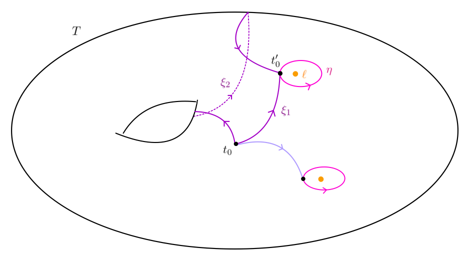
Figure 3. Simple loops around Landau components.

Note that simple loops become contractible under the inclusion $T\setminus L\rightarrow T$. In fact, simple loops generate the entire kernel of the corresponding surjection

(3.1) $$\pi_{1}(T\setminus L,t_{0})\twoheadrightarrow\pi_{1}(T,t_{0})$$

of fundamental groups of $T\setminus L$, for any base point $t_{0}\in T\setminus L$ (see appendix D). Picard-Lefschetz theory determines the variation along small loops, but says nothing about loops that remain non-trivial in $\pi_{1}(T,t_{0})$. The latter emerge from the global topology of $T$, whereas the former arise from the degeneration of the fibres of $\pi$ over a critical point $t_{c}\in L$, and are in this sense local in $T$.

Example 3.2.

In fig. 3 the loops $\xi_{1}^{-1}\star\eta\star\xi_{1}$ and $\xi_{2}^{-1}\star\eta\star\xi_{2}$ are two non-homotopic simple loops. The loop $\xi_{1}^{-1}\star\xi_{2}$ is not simple, because it is non-trivial in the fundamental group of the torus $T\cong\mathbb{S}^{1}\times\mathbb{S}^{1}$.

Let $\mathfrak{L}$ denote the set of irreducible components $\ell\subseteq L$ of complex codimension one in $T$. Since we are only concerned with small loops, we can replace $T$ with a disk $\mathbb{D}=\{\lvert t_{1}\rvert<2\}\subset\mathbb{C}$ of complex dimension one in a suitable coordinate $t_{1}$. This disk embeds transverse to some component $\ell\in\mathfrak{L}$ such that $\mathbb{D}\cap L=\{t_{c}\}$ is a single point of $\ell$. By 3.1, $t_{c}$ is a smooth point of $\ell$, so that, in particular, $t_{c}\notin\ell\cap\ell^{\prime}$ for any other component $\ell\neq\ell^{\prime}\in\mathfrak{L}$.

Since $\pi$ is a proper submersion and hence $Y\rightarrow T$ a fibre bundle, this localization in $T$ also implies that we can assume that $Y\cong X\times T$ is trivial as a smooth manifold, with $X$ a smooth compact manifold and $\pi(x,t)=t$.

In fact, in this section we will only consider variations around Landau singularities $\ell\in\mathfrak{L}$ that emerge from fibrewise isolated critical points: We assume that over the point $t_{c}\in\ell$, the critical sets $cS\cap\pi^{-1}(t_{c})$ consist of isolated points, for each stratum $S\in\mathfrak{S}$. In section 3.2 we show that this leads to a further localization, this time in $X$, to neighbourhoods of precisely those isolated points in the critical fibre. After this second localization, we may assume that $Y\cong X\times T$, with $\pi(x,t)=t$, also as a complex manifold.

3.1. Monodromy and variation

Let $\gamma\colon[0,1]\rightarrow T\setminus L$ be a closed path based at $\gamma(0)=\gamma(1)=t_{0}$. Since $\pi|_{{\pi}^{-1}(T\setminus L)}$ is a pair of fibre bundles (2.5), the pullback bundle $\gamma^{*}\pi$ over the contractible interval $[0,1]$ is trivial. Hence one can find a continuous family $g_{\tau}\colon Y_{t_{0}}\rightarrow Y_{\gamma(\tau)}$ of homeomorphisms, which furthermore restrict to homeomorphisms $g_{\tau}|_{S}\colon S_{t_{0}}\rightarrow S_{\gamma(\tau)}$ of the fibres of every stratum $S\in\mathfrak{S}$ of $A\cup B$. The induced homeomorphisms

$$(Y_{t_{0}}\setminus A_{t_{0}},B_{t_{0}}\setminus A_{t_{0}})\longrightarrow(Y_{\gamma(\tau)}\setminus A_{\gamma(\tau)},B_{\gamma(\tau)}\setminus A_{\gamma(\tau)})$$

of pairs are well-defined up to homotopy, and depend (up to homotopy) only on the homotopy class of $\gamma$. Hence on the level of the homology groups

$$H_{\bullet}(t)=H_{\bullet}(Y_{t}\setminus A_{t},B_{t}),$$

the pushforward of $g_{\tau}$ (restricted to $Y_{t_{0}}\setminus A_{t_{0}}$) is independent of the choice of the trivialization $g$ of $\gamma^{*}\pi$. We denote this pushforward of $g_{1}$ by

$$\gamma_{*}\colon H_{\bullet}(t_{0})\longrightarrow H_{\bullet}(t_{0}).$$

This map depends only on the homotopy class of $\gamma$. The assignment $\gamma\mapsto\gamma_{*}$ defines an action of the fundamental group $\pi_{1}(T\setminus L,t_{0})$ on the homology group $H_{\bullet}(t_{0})$, called the monodromy representation.

Definition 3.3.

The variation operators on the homology group of a fibre measure the difference between the monodromy and the identity:

(3.2) $$\operatorname{Var}_{\gamma}\colon H_{\bullet}(t_{0})\longrightarrow H_{\bullet}(t_{0}),\quad h\longmapsto\gamma_{*}h-h.$$

Remark 3.4.

If the fibres $Y_{t}=X$ are constant ($Y=X\times T$), then a trivialization $g$ of $\gamma^{*}\pi$ provides an ambient isotopy $g_{1}$ of $(A\cup B)_{t_{0}}$ in $X$ that preserves each stratum individually. An ambient isotopy of a subspace $M\subseteq X$ is a homeomorphism $\phi\colon M\rightarrow M$ that can be extended to a continuous family $(g_{\tau})_{0\leq\tau\leq 1}$ of homeomorphisms $g_{\tau}\colon X\to X$, such that $g_{0}=\mathrm{id}$ and $g_{1}|_{M}=\phi$.

Since we assume that $A\cup B$ has at worst simple normal crossing singularities, we can in fact find an ambient isotopy in the smooth category (provided that the path $\gamma$ is smooth). This follows from 2.6, and means that the trivialization $g\colon X\times[0,1]\rightarrow X$ can be chosen to be smooth and such that each $g_{\tau}\colon X\rightarrow X$ is a diffeomorphism. Such an isotopy is also called a diffeotopy [30].

Example 3.5.

Consider projective space $X=\mathbb{P}^{1}$ over the base $T=\mathbb{C}$, with $B=\varnothing$ and remove $A=A_{1}\cup A_{2}$ where $A_{1}=\{x=\infty\}$ and $A_{2}=\{x^{2}=t\}$. All fibres $X\setminus A_{t}=\mathbb{C}\setminus\{\sqrt{t},-\sqrt{t}\}$ over $t\neq 0$ are isomorphic via $x\mapsto x/\sqrt{t}$ to $X\setminus A_{t=1}=\mathbb{C}\setminus\{1,-1\}$. This trivialization lifts the loop $t=\gamma(\tau)=e^{2\mathrm{i}\pi\tau}$ around the Landau variety $L=\{0\}$ to the diffeotopy $g_{\tau}(x)=x\cdot e^{\mathrm{i}\pi\tau}$. The latter ends in the antipode $g_{1}(x)=-x$, which swaps the punctures $\pm 1$ in the fibre over $t_{0}=1$. Let $\sigma_{\pm}$ be two loops around $\pm 1$. They generate $H_{1}(t_{0})\cong\mathbb{Z}^{2}$ and the monodromy $\gamma_{*}$ swaps them, $\gamma_{*}(\sigma_{\pm})=\sigma_{\mp}$, see fig. 4. Hence, the variation is

$$\operatorname{Var}_{\gamma}(\sigma_{+})=-\operatorname{Var}_{\gamma}(\sigma_{-})=\sigma_{-}-\sigma_{+}.$$

Figure 4. Isotopy for $A=\{x^{2}=t\}\subset\mathbb{C}$ by rotation swaps the loops $\sigma_{\pm}$ (3.5).

Example 3.6.

Consider $X=\mathbb{P}^{1}$, $A=\{x=t,\infty\}$ and $B=\{x=0,2\}$ over the loop $t=\gamma(\tau)=e^{2\mathrm{i}\pi\tau}$ (see fig. 9). The trivialization $(X\setminus A,B)_{\gamma(\tau)}\cong(\mathbb{C}\setminus\{1\},\{0,2\})$ given by $g_{\tau}(x)=xe^{2\mathrm{i}\pi\tau}$ yields the isotopy $g_{\gamma}(x)=x$. Let $t_{0}=1$. Choose a path $\sigma$ in $\mathbb{C}\setminus\{1\}$ from $0$ to $2$, and let $\delta\{1\}$ as above. Then $H(t_{0})\cong\mathbb{Z}^{2}$ is generated by (the classes of) $\sigma$ and $\delta\{1\}$, and the monodromy $\gamma_{*}$ maps $\delta\{1\}$ to itself and $\sigma$ to $\sigma-\delta\{1\}$. Thus,

$$\operatorname{Var}_{\gamma}(\delta\{1\})=0,\qquad\operatorname{Var}_{\gamma}(\sigma)=-\delta\{1\}.$$

3.2. Localization

A crucial property of the variation operators is that both their domain and codomain can be localized near the critical points over $\ell$.

In order to define a local variation operation, we need to show that if we are able to localize the critical sets $cS$ of all strata inside an open submanifold $W\subseteq X$, then the isotopy $g_{\gamma}$ can be chosen to be the identity outside $W$. Note that for fibrewise isolated critical points such a $W$ always exists by Milnor’s theorem [43]—take for instance the union of small open balls around each critical point. If $\cup_{S\in\mathfrak{S}}cS$ is not isolated (fibrewise), but still smooth, then we can construct $W$ by taking small tubular neighbourhoods of the critical sets in a fibre.

Lemma 3.7.

Let $W$ be an open submanifold of $X$ such that $\partial W$ is smooth and transverse to $A\cup B$, and such that $W$ contains the critical sets of all strata of $A_{t}\cup B_{t}$, for all $t$ in a small disk near $t_{c}\in L$. Then the ambient isotopy $g_{\gamma}\colon(X\setminus A_{t},B_{t}\setminus A_{t})\to(X\setminus A_{t},B_{t}\setminus A_{t})$ is homotopic to a map that is the identity outside of $W$.

Proof.

This is a special instance of the isotopy extension theorem [30, §8].

Let $C$ denote the union of all critical sets $cS$ in the fiber over $t_{c}\in L$. Using a collar neighbourhood of $\partial W$ we can construct a closed submanifold $W^{\prime}\subset W$ that contains $C$ and whose boundary $\partial W^{\prime}$ is also transverse to all strata of $A\cup B$. This transversality implies that adding $\partial W$ and $\partial W^{\prime}$ to the arrangement $A\cup B$ does not alter the associated Landau variety. From 2.5 and 2.6 we obtain thus a smooth stratum preserving trivialization $h$ that gives rise to (see 3.4) a smooth ambient isotopy $g_{\gamma}\colon(X\setminus A_{t},B_{t}\setminus A_{t})\to(X\setminus A_{t},B_{t}\setminus A_{t})$. The crucial point here is that this map fixes $\partial W^{\prime}$ (globally).

Let $g_{\tau}$ be a realization of $g_{\gamma}$, that is, a family of (stratum preserving) diffeomorphisms $g_{\tau}\colon X\to X$ and subsets $S_{\tau}\subseteq X$ with $S_{0}=S_{1}=A_{t}\cup B_{t}\cup\partial W\cup\partial W^{\prime}$, such that $g_{0}=\operatorname{id}_{X}$, $g_{1}=g_{\gamma}$ and $g_{\tau}|_{S_{0}}\colon S_{0}\cong S_{\tau}$. The track of $g$ is the diffeomorphism

$$G\colon I\times X\longrightarrow I\times X,\quad(\tau,x)\longmapsto(\tau,g_{\tau}(x)).$$

Let $V$ be the velocity field of $G$, the vector field on $I\times X$, tangential to the curves $\tau\mapsto(\tau,g_{\tau}(x))$. Identifying $T(\mathbb{R}\times X)$ with $T(\mathbb{R})\oplus T(X)$ it has the form $V(\tau,x)=\frac{\partial}{\partial\tau}+v(\tau,x)$ where $v(\tau,x)$ is a vector field on $X$. In this way every ambient isotopy gives rise to a time-dependent vector field on $X$. The reverse statement is also true if the time-dependent vector field is compactly supported. In our case $X$ is compact, so this condition is automatically satisfied. Moreover, observe that $V$ is tangential to the set $S=\{(\tau,x)\mid x\in S_{\tau}\}\subseteq I\times X$, hence its flow (which is $G$) leaves $S$ invariant.

Since $C$ is contained in $W^{\prime}$, the ambient isotopy $g_{\gamma}$ will be homotopic to the identity map on its complement $X\setminus W^{\prime}$. Let $V_{\lambda}(\tau,x)$ be the associated homotopy of vector fields on $I\times(X\setminus W^{\prime})$ (between $V_{0}(\tau,x)=V(\tau,x)|_{x\in X\setminus W^{\prime}}$ and the constant vector field $V_{1}(\tau,x)=\frac{\partial}{\partial\tau}$, whose flow induces the identity map). Choose a partition of unity $\{\rho_{1},\rho_{2}\}$, subordinate to the open cover $U_{1}\cup U_{2}=X$ with $U_{1}=W$ and $U_{2}=X\setminus W^{\prime}$, and define a vector field $F_{\lambda}$ on $I\times X$ by $F_{\lambda}(\tau,x)=\rho_{1}(x)V(\tau,x)+\rho_{2}(x)V_{\lambda}(\tau,x)$. Let $f_{\lambda}$ be the ambient isotopy induced by $F_{\lambda}$. Then

• $f_{\lambda}|_{S_{0}}\colon S_{0}\cong S_{1}$ for each $\lambda\in[0,1]$,

• $f_{\lambda}$ is a homotopy between $f_{1}$ and $f_{0}=g_{\gamma}$,

• $f_{1}$ is equal to $g_{\gamma}$ on $W^{\prime}$,

• $f_{1}$ is the identity outside of $W$.

∎

Example 3.8.

The isotopy $g_{\gamma}(x)=-x$ from 3.5 is not the identity outside of $W=\{\lvert x\rvert<1\}\subset\mathbb{C}$. Pick any smooth function $\rho\colon\mathbb{R}\rightarrow[0,1]$ with $\rho(r)=1$ for $r\geq 1$ and $\rho(r)=0$ for $r\leq 1/2$. Then the diffeomorphisms $\phi_{\tau}(x)=x\cdot e^{\mathrm{i}\pi\tau\rho(\lvert x\rvert)}$ restrict to $x\mapsto x\cdot e^{\mathrm{i}\pi\tau}$ outside $W$, and to the identity inside the smaller ball $W^{\prime}=\{\lvert x\rvert<1/2\}$. In particular, $\phi_{\tau}$ fixes the stratum $S=\{x^{2}=t\}\subseteq W^{\prime}$ and thereby defines a diffeotopy of the pair $(\mathbb{C},S_{t})$. This family $\phi_{\tau}$ is smooth in $\tau$, so $\phi_{1}$ is homotopic to $\phi_{0}=\operatorname{id}$. It follows that $g_{\gamma}\simeq f$ is homotopic the composition $f(x)=\phi_{1}g_{\gamma}(x)=x\cdot e^{\mathrm{i}\pi(1-\rho(\lvert x\rvert))}$ which has the desired property that $f|_{W^{\mathsf{c}}}=\operatorname{id}$ (fig. 5).

Figure 5. 3.8 of an ambient isotopy $f=\phi_{1}g_{\gamma}$ that is the identity outside of $W$ and homotopic to $g_{\gamma}(x)=-x$. Here $S=\{x^{2}=t\}\subset\mathbb{C}$ and $\phi_{1}|_{W^{\prime}}=\operatorname{id}$, $\phi_{1}|_{W^{\mathsf{c}}}=-\operatorname{id}$.

By 3.7, the variation of a class $h\in H_{\bullet}(t_{0})$ can be represented by a cycle contained in $W\setminus A_{t_{0}}$ with boundary in $W\cap B_{t_{0}}$, and furthermore this variation $\operatorname{Var}_{\gamma}h$ depends only on how $h$ intersects the closed ball $\overline{W}$. To make this precise, let $W^{\mathsf{c}}=X\setminus W$ denote the complement of the ball and consider the following map, induced by an inclusion of pairs:

(3.3) $$H_{\bullet}(\overline{W}\setminus A_{t},\partial W\cup B_{t})\longrightarrow H_{\bullet}(X\setminus A_{t},W^{\mathsf{c}}\cup B_{t}).$$

Lemma 3.9.

The map (3.3) is an isomorphism.

Proof.

Extend the inclusion $\partial W\hookrightarrow W^{\mathsf{c}}$ of the boundary to some collar neighbourhood $u\colon\partial W\times[0,1)\cong U\subset W^{\mathsf{c}}$.

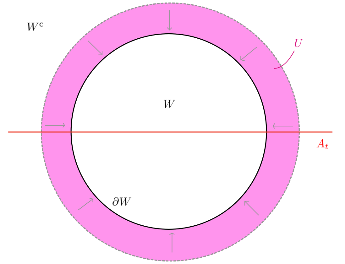
Figure 6. Collar neighbourhood $U\cong[0,1)\times\partial W\subset W^{\mathsf{c}}$ used for the excision argument in the proof of 3.9.

Adding the collar $U$, we can thicken $W$ into $W^{\prime}=W\cup U$ and excise $W^{\mathsf{c}}\setminus(W^{\prime}\cup A_{t})$ from the pair $(X\setminus A_{t},W^{\mathsf{c}}\cup B_{t}\setminus A_{t})$, to replace it with the pair $(W^{\prime}\setminus A_{t},U\cup B_{t}\setminus A_{t})$; see fig. 6. Since $\partial W\cup A_{t}\cup B_{t}$ intersect transversely, we can choose $u$ in such a way that it preserves $A$ and $B$ (see appendix B). For the corresponding projection $r\colon U\rightarrow\partial W$, this means $r(U\cap A_{t})=\partial W\cap A_{t}$ and $r(U\cap B_{t})=\partial W\cap B_{t}$. Note that $r$ fixes $\partial W$ pointwise, so we can extend $r$ to a map $r\colon W^{\prime}\rightarrow\overline{W}$ by setting $r|_{W}=\operatorname{id}_{W}$ and this still preserves $A_{t}$ and $B_{t}$. This $r$ descends to deformation retractions $(U\cup B_{t})\setminus A_{t}\rightarrow(\partial W\cup B_{t})\setminus A_{t}$ and $W^{\prime}\setminus A_{t}\rightarrow\overline{W}\setminus A_{t}$. ∎

Definition 3.10.

The $W$-trace or trace-in-the-ball [21] is the homomorphism

(3.4) $$W_{*}\colon H_{\bullet}(X\setminus A_{t},B_{t})\longrightarrow H_{\bullet}(\overline{W}\setminus A_{t},\partial W\cup B_{t})$$

given by the map of pairs $H_{\bullet}(X\setminus A_{t},B_{t})\rightarrow H_{\bullet}(X\setminus A_{t},W^{\mathsf{c}}\cup B_{t})$ and the isomorphism (3.3). We further write $\iota\colon(W\setminus A_{t},W\cap B_{t}\setminus A_{t})\rightarrow(X\setminus A_{t},B_{t}\setminus A_{t})$ for the natural inclusion of pairs, and denote its push-forward $\iota_{*}$.

Proposition 3.11.

Suppose that $g_{\gamma}$ is the identity map outside of $W$. Then $g_{\gamma}$ canonically determines a homomorphism

(3.5) $$\operatorname{var}_{\gamma}\colon H_{\bullet}(\overline{W}\setminus A_{t},\partial W\cup B_{t})\longrightarrow H_{\bullet}(W\setminus A_{t},B_{t})$$

such that the following diagram for $\operatorname{Var}_{\gamma}=g_{\gamma*}-\operatorname{id}$ commutes:

(3.6) $$\begin{gathered}\lx@xy@svg{\hbox{\raise 0.0pt\hbox{\kern 46.84924pt\hbox{\ignorespaces\ignorespaces\ignorespaces\hbox{\vtop{\kern 0.0pt\offinterlineskip\halign{\entry@#!@&&\entry@@#!@\cr&&\\&&\\}}}\ignorespaces{\hbox{\kern-35.53502pt\raise 0.0pt\hbox{\hbox{\kern 0.0pt\raise 0.0pt\hbox{\hbox{\kern 3.0pt\raise 0.0pt\hbox{$\textstyle{H_{\bullet}(X\setminus A_{t},B_{t})\ignorespaces\ignorespaces\ignorespaces\ignorespaces\ignorespaces\ignorespaces\ignorespaces\ignorespaces}$}}}}}}}\ignorespaces\ignorespaces\ignorespaces\ignorespaces{}{\hbox{\lx@xy@droprule}}\ignorespaces\ignorespaces\ignorespaces{\hbox{\kern 0.0pt\raise-20.0pt\hbox{{}\hbox{\kern 0.0pt\raise 0.0pt\hbox{\hbox{\kern 3.0pt\hbox{\hbox{\kern 0.0pt\raise-1.92639pt\hbox{$\scriptstyle{W_{\ast}}$}}}\kern 3.0pt}}}}}}\ignorespaces{\hbox{\kern 0.0pt\raise-29.5pt\hbox{\hbox{\kern 0.0pt\raise 0.0pt\hbox{\lx@xy@tip{1}\lx@xy@tip{-1}}}}}}{\hbox{\lx@xy@droprule}}{\hbox{\lx@xy@droprule}}\ignorespaces\ignorespaces\ignorespaces\ignorespaces{}{\hbox{\lx@xy@droprule}}\ignorespaces\ignorespaces\ignorespaces{\hbox{\kern 58.8518pt\raise 6.2111pt\hbox{{}\hbox{\kern 0.0pt\raise 0.0pt\hbox{\hbox{\kern 3.0pt\hbox{\hbox{\kern 0.0pt\raise-1.57222pt\hbox{$\scriptstyle{\operatorname{Var}_{\gamma}}$}}}\kern 3.0pt}}}}}}\ignorespaces{\hbox{\kern 101.7312pt\raise 0.0pt\hbox{\hbox{\kern 0.0pt\raise 0.0pt\hbox{\lx@xy@tip{1}\lx@xy@tip{-1}}}}}}{\hbox{\lx@xy@droprule}}{\hbox{\lx@xy@droprule}}{\hbox{\kern 70.84924pt\raise 0.0pt\hbox{\hbox{\kern 0.0pt\raise 0.0pt\hbox{\hbox{\kern 3.0pt\raise 0.0pt\hbox{$\textstyle{}$}}}}}}}{\hbox{\kern 101.7312pt\raise 0.0pt\hbox{\hbox{\kern 0.0pt\raise 0.0pt\hbox{\hbox{\kern 3.0pt\raise 0.0pt\hbox{$\textstyle{H_{\bullet}(X\setminus A_{t},B_{t})}$}}}}}}}{\hbox{\kern-46.84924pt\raise-40.0pt\hbox{\hbox{\kern 0.0pt\raise 0.0pt\hbox{\hbox{\kern 3.0pt\raise 0.0pt\hbox{$\textstyle{H_{\bullet}(\overline{W}\setminus A_{t},\partial W\cup B_{t})\ignorespaces\ignorespaces\ignorespaces\ignorespaces}$}}}}}}}\ignorespaces\ignorespaces\ignorespaces\ignorespaces{}{\hbox{\lx@xy@droprule}}\ignorespaces\ignorespaces\ignorespaces{\hbox{\kern 59.82402pt\raise-34.67361pt\hbox{{}\hbox{\kern 0.0pt\raise 0.0pt\hbox{\hbox{\kern 3.0pt\hbox{\hbox{\kern 0.0pt\raise-0.6875pt\hbox{$\scriptstyle{\operatorname{var}_{\gamma}}$}}}\kern 3.0pt}}}}}}\ignorespaces{\hbox{\kern 100.84924pt\raise-40.0pt\hbox{\hbox{\kern 0.0pt\raise 0.0pt\hbox{\lx@xy@tip{1}\lx@xy@tip{-1}}}}}}{\hbox{\lx@xy@droprule}}{\hbox{\lx@xy@droprule}}{\hbox{\kern 70.84924pt\raise-40.0pt\hbox{\hbox{\kern 0.0pt\raise 0.0pt\hbox{\hbox{\kern 3.0pt\raise 0.0pt\hbox{$\textstyle{}$}}}}}}}{\hbox{\kern 100.84924pt\raise-40.0pt\hbox{\hbox{\kern 0.0pt\raise 0.0pt\hbox{\hbox{\kern 3.0pt\raise 0.0pt\hbox{$\textstyle{H_{\bullet}(W\setminus A_{t},B_{t})\ignorespaces\ignorespaces\ignorespaces\ignorespaces}$}}}}}}}\ignorespaces\ignorespaces\ignorespaces\ignorespaces{}{\hbox{\lx@xy@droprule}}\ignorespaces\ignorespaces\ignorespaces{\hbox{\kern 137.26622pt\raise-20.0pt\hbox{{}\hbox{\kern 0.0pt\raise 0.0pt\hbox{\hbox{\kern 3.0pt\hbox{\hbox{\kern 0.0pt\raise-1.04167pt\hbox{$\scriptstyle{\iota_{\ast}}$}}}\kern 3.0pt}}}}}}\ignorespaces{\hbox{\kern 137.26622pt\raise-5.5pt\hbox{\hbox{\kern 0.0pt\raise 0.0pt\hbox{\lx@xy@tip{1}\lx@xy@tip{-1}}}}}}{\hbox{\lx@xy@droprule}}{\hbox{\lx@xy@droprule}}\ignorespaces}}}}\ignorespaces\end{gathered} \textstyle{H_{\bullet}(X\setminus A_{t},B_{t})\ignorespaces\ignorespaces\ignorespaces\ignorespaces\ignorespaces\ignorespaces\ignorespaces\ignorespaces} \scriptstyle{W_{\ast}} \scriptstyle{\operatorname{Var}_{\gamma}} \textstyle{H_{\bullet}(X\setminus A_{t},B_{t})} \textstyle{H_{\bullet}(\overline{W}\setminus A_{t},\partial W\cup B_{t})\ignorespaces\ignorespaces\ignorespaces\ignorespaces} \scriptstyle{\operatorname{var}_{\gamma}} \textstyle{H_{\bullet}(W\setminus A_{t},B_{t})\ignorespaces\ignorespaces\ignorespaces\ignorespaces} \scriptstyle{\iota_{\ast}} \textstyle{H_{\bullet}(X\setminus A_{t},B_{t})\ignorespaces\ignorespaces\ignorespaces\ignorespaces\ignorespaces\ignorespaces\ignorespaces\ignorespaces} \scriptstyle{W_{\ast}} \scriptstyle{\operatorname{Var}_{\gamma}} \textstyle{H_{\bullet}(X\setminus A_{t},B_{t})} \textstyle{H_{\bullet}(\overline{W}\setminus A_{t},\partial W\cup B_{t})\ignorespaces\ignorespaces\ignorespaces\ignorespaces} \scriptstyle{\operatorname{var}_{\gamma}} \textstyle{H_{\bullet}(W\setminus A_{t},B_{t})\ignorespaces\ignorespaces\ignorespaces\ignorespaces} \scriptstyle{\iota_{\ast}}$$

Proof.

The triple $B_{t}\setminus A_{t}\subset(B_{t}\cup W^{\mathsf{c}})\setminus A_{t}\subset X\setminus A_{t}$ gives a long exact sequence that identifies the kernel of $W_{*}$ with the image of

$$j_{*}\colon H_{\bullet}((B_{t}\cup W^{\mathsf{c}})\setminus A_{t},B_{t})\longrightarrow H_{\bullet}(X\setminus A_{t},B_{t}).$$

Analogously to the proof of 3.9, we can excise all of $\overline{W}\cap B_{t}\setminus A_{t}$ from the domain of $j_{*}$, except for a layer $U\cap B_{t}\setminus A_{t}\cong[0,1)\times(\partial W\cap B_{t}\setminus A_{t})$ in a collar neighbourhood of $\partial W$ inside $W$ (fig. 7).

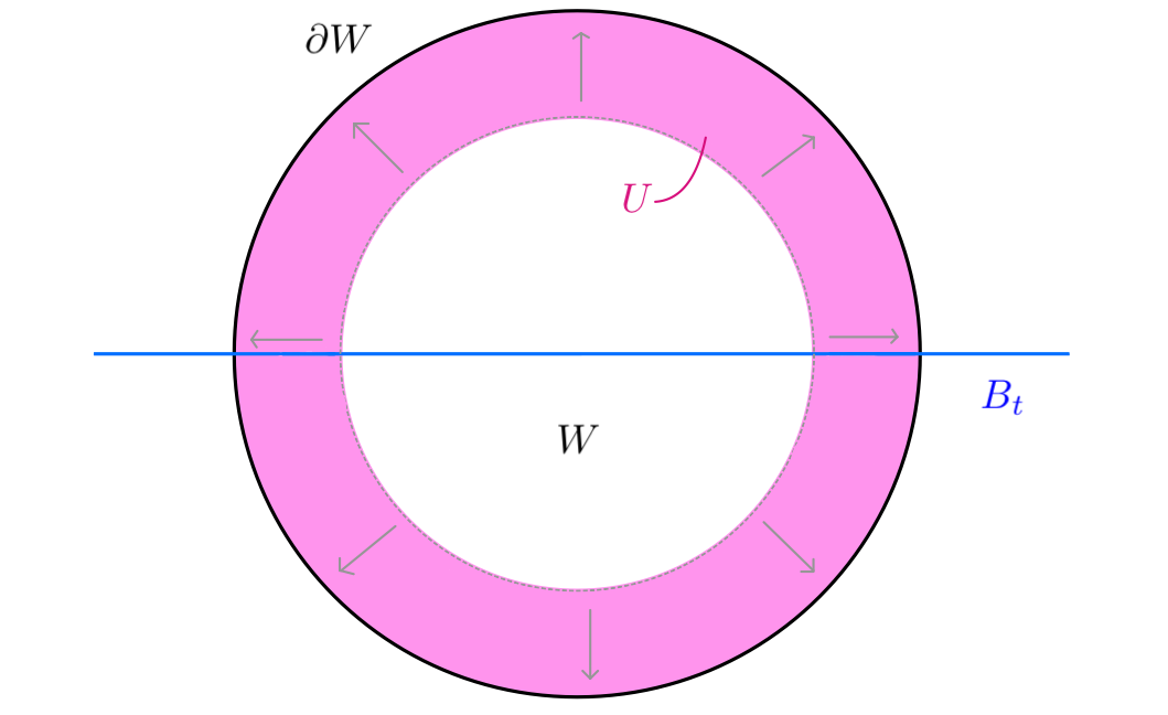
Figure 7. Collar neighbourhood $U\cong[0,1)\times\partial W\subset\overline{W}$ used for the excision argument in the proof of 3.11.

The deformation retraction

$$U\cap B_{t}\setminus A_{t}\longrightarrow\partial W\cap B_{t}\setminus A_{t}$$

then identifies the domain of $j_{*}$ with $H_{\bullet}(W^{\mathsf{c}}\setminus A_{t},B_{t})$. Every $h\in\ker W_{*}$ can thus be written as $h=j_{*}\sigma$ where $\sigma\in H_{\bullet}(W^{\mathsf{c}}\setminus A_{t},B_{t})$ has support inside $W^{\mathsf{c}}$. This has variation

$$\operatorname{Var}_{\gamma}h=(g_{\gamma*}-\operatorname{id})j_{*}\sigma=j_{*}(g_{\gamma}|_{W^{\mathsf{c}}\setminus A_{t}}-\operatorname{id})_{*}\sigma=j_{*}0\sigma=0,$$

and we conclude that indeed, $\operatorname{Var}_{\gamma}$ factors through $W_{*}$. Now consider again the thicker $W^{\prime}\supset W$ from 3.9. Since $X=W^{\prime}\cup(X\setminus\overline{W})$ is an open cover, we can represent every $h\in H_{\bullet}(X\setminus A_{t},B_{t})$ by a chain $h=x+y$ with $x$ and $y$ supported in $W^{\prime}\setminus A_{t}$ and $X\setminus(\overline{W}\cup A_{t})$, respectively. Since $g_{\gamma*}y=y$, we see that $\operatorname{Var}_{\gamma}h=g_{\gamma*}x-x$ takes values in $H_{\bullet}(W^{\prime}\setminus A_{t},B_{t})$. But $H_{\bullet}(W\setminus A_{t},B_{t})\rightarrow H_{\bullet}(W^{\prime}\setminus A_{t},B_{t})$ is an isomorphism, because the deformation retracts $W^{\prime}\rightarrow\overline{W}\rightarrow\overline{W}\setminus U\subseteq W$ (from 3.9 and the above collar $U$ inside $W$) are compatible with $A_{t}$ and $B_{t}$. This proves the factorization of $\operatorname{Var}_{\gamma}$ through $\iota_{*}$. ∎

Here it is important to note that $\operatorname{var}_{\gamma}$ is not simply a localized version of $\operatorname{Var}_{\gamma}$; it does not carry the same information. The crucial point is that the latter factorizes by means of $W_{*}$ and $\operatorname{var}_{\gamma}$, not that local and global variations are necessarily equal. See 3.5/fig. 8 and 3.6/fig. 9 for examples where the two are indeed different. These highlight a general fact that holds for the simple pinch singularities that we consider in the next section: For linear pinches the variation always vanishes in $H_{\bullet}(\overline{W}\setminus A,\partial W\cup B)$, for quadratic pinches the variation vanishes if $n-m$ is odd.

$g_{\gamma_{*}}(h)=$ $\cong$

$g_{\gamma_{*}}(\color[rgb]{0.0750000000000001,0.925,0}W_{*}h\color[rgb]{0,0,0})=\$ $\quad\cong\$

Figure 8. Global vs. local monodromy: For a quadratic pinch $A=\{x^{2}=t\}$ and $\gamma$ a small loop around $t=0$ the variation $\operatorname{Var}_{\gamma}$ of $h\in H_{\bullet}(X\setminus A)$ is given by the vanishing cycle $\nu\in H_{\bullet}(W\setminus A)$ (top right). The variation of $W_{*}h$ is $-2W_{*}h$ which is homologous to $\nu$ in $H_{\bullet}(\overline{W}\setminus A,\partial W)$, but not in $H_{\bullet}(\overline{W}\setminus A)$ (bottom right).

$g_{\gamma_{*}}(h)=$ $\cong$

$g_{\gamma_{*}}(\color[rgb]{0.0750000000000001,0.925,0}W_{*}h\color[rgb]{0,0,0})=$ $\ \cong$

Figure 9. Global vs. local monodromy: For a linear pinch $A=\{x=t\}$, $B=\{x=0,2\}$ and $\gamma$ a small loop around $t=0$ the variation $\operatorname{Var}_{\gamma}$ of $h\in H_{\bullet}(X\setminus A,B)$ is given by the vanishing cycle $\nu\in H_{\bullet}(W\setminus A)$ (top right). However, the variation of $W_{*}h$ in $H_{\bullet}(\overline{W}\setminus A,\partial W\cup B)$ vanishes (bottom right).

Remark 3.12.

All of the above remains valid in the special cases $A=\varnothing$ or $B=\varnothing$. Furthermore, it holds also if we replace $X\setminus A_{t_{0}}$ by other subsets of $X$ such as intersections, unions and complements of elements of $\mathfrak{A}$ and $\mathfrak{B}$.

3.3. Simple pinch singularities

The Picard-Lefschetz formulas from [21, 51] apply only where the degeneration of $A\cup B$ over $L$ is sufficiently benign. They require that the neighbourhoods of the critical points can be modelled by hypersurface arrangements of the following types (we comment on generalizations in section 3.9).

Definition 3.13.

Consider a critical point $p\in cS$ of the stratified map $\pi$, on some stratum $S\subseteq D_{1}\cap\ldots\cap D_{m}$ with complex codimension $m\leq n+1$. Then $p$ is called a linear ($m=n+1$) or quadratic ($m\leq n$) simple pinch if there exist holomorphic local coordinates $t=(t_{1},\ldots,t_{q})$ at $\pi(p)\in T$ and $y=(x,t)\colon U\rightarrow\mathbb{C}^{n+q}$ at $p\in U\subseteq Y$, trivializing $\pi(x,t)=t$, such that the hypersurfaces $D_{i}\cap U\cong S_{i}\cap y(U)$ take the form

(3.7) $$\begin{split}S_{i}&=\{x_{i}=0\},\quad\text{for}\quad i=1,\ldots,m-1,\\ S_{m}&=\{x_{1}+\ldots+x_{m-1}+x_{m}^{2}+\ldots+x_{n}^{2}=t_{1}\}.\end{split}$$

These hypersurfaces $\{S_{1},\ldots,S_{m}\}$ are smooth and intersect transversely. There are no critical points $c(S^{I})=\varnothing$ on the intersections $S^{I}=\bigcap_{i\in I}S_{i}$ of a proper subset $I\subset\{1,\ldots,m\}$. The only critical stratum is the intersection of all $m$ hypersurfaces. Its critical set

($$\sharp c(S^{1,\ldots,m})=\{x=0\}\cap\{t_{1}=0\}=\{(0,\ldots,0,t_{2},\ldots,t_{q})\}$$)

is smooth and projects isomorphically onto the Landau variety $\{t_{1}=0\}$; each fibre with $t_{1}=0$ has a unique critical point with coordinates $(0,t)$.

For a linear simple pinch, the fibres of $S^{1,\ldots,n+1}=cS^{1,\ldots,n+1}$ are empty over $t_{1}\neq 0$, and consist of a single point (the critical point) over $t_{1}=0$.

For a quadratic simple pinch, each fibre of the stratum $S^{1,\ldots,m}$, over $t$ with $t_{1}\neq 0$, contains a real sphere

$$\mathbb{S}^{n-m}=\{u\in\mathbb{R}^{n-m+1}\colon\lVert u\rVert=1\},$$

embedded as $u\mapsto(0,\ldots,0,u\cdot\sqrt{t_{1}},t)$. As $t_{1}\rightarrow 0$, these spheres shrink and eventually collapse, over $t_{1}=0$, to a point (the critical point). They are therefore called vanishing spheres.

Definition 3.14.

A simple critical value is a point $t\in L$ such that all critical points in the fibre $\pi^{-1}(t)$ are linear or quadratic simple pinches.

A simple pinch component of $L$ is a component $\ell\in\mathfrak{L}$ such that a generic point $t\in\ell$ is simple.

Suppose $t_{c}\in L$ is a simple critical value, and denote $P=\pi^{-1}(t_{c})\cap\bigcup_{S\in\mathfrak{S}}cS$ the corresponding simple pinches. Every $p\in P$ is an isolated critical point in the compact fibre $Y_{t_{c}}$, hence $P$ is finite. Pick a chart $y_{p}\colon U_{p}\rightarrow\mathbb{C}^{n+q}$ of the form (3.7) for each $p$, centred at $y_{p}(p)=(0,0)$. By rescaling these coordinates, and shrinking the neighbourhoods $U_{p}$, we can ensure that (fig. 10):

• $U_{p}$ and $U_{p^{\prime}}$ are disjoint when $p\neq p^{\prime}$,

• the chart $y_{p}(U_{p})$ contains the closure $\overline{W}\times\{0\}$ of the open ball

  $$W=\{\lVert x\rVert^{2}=\lvert x_{1}\rvert^{2}+\ldots+\lvert x_{n}\rvert^{2}<1\}\subset\mathbb{C}^{n}.$$

• the only hypersurfaces $D_{i}\in\mathfrak{D}$ that intersect $U_{p}$ are those that contain $p$ (that is, those that correspond to the $S_{i}$).

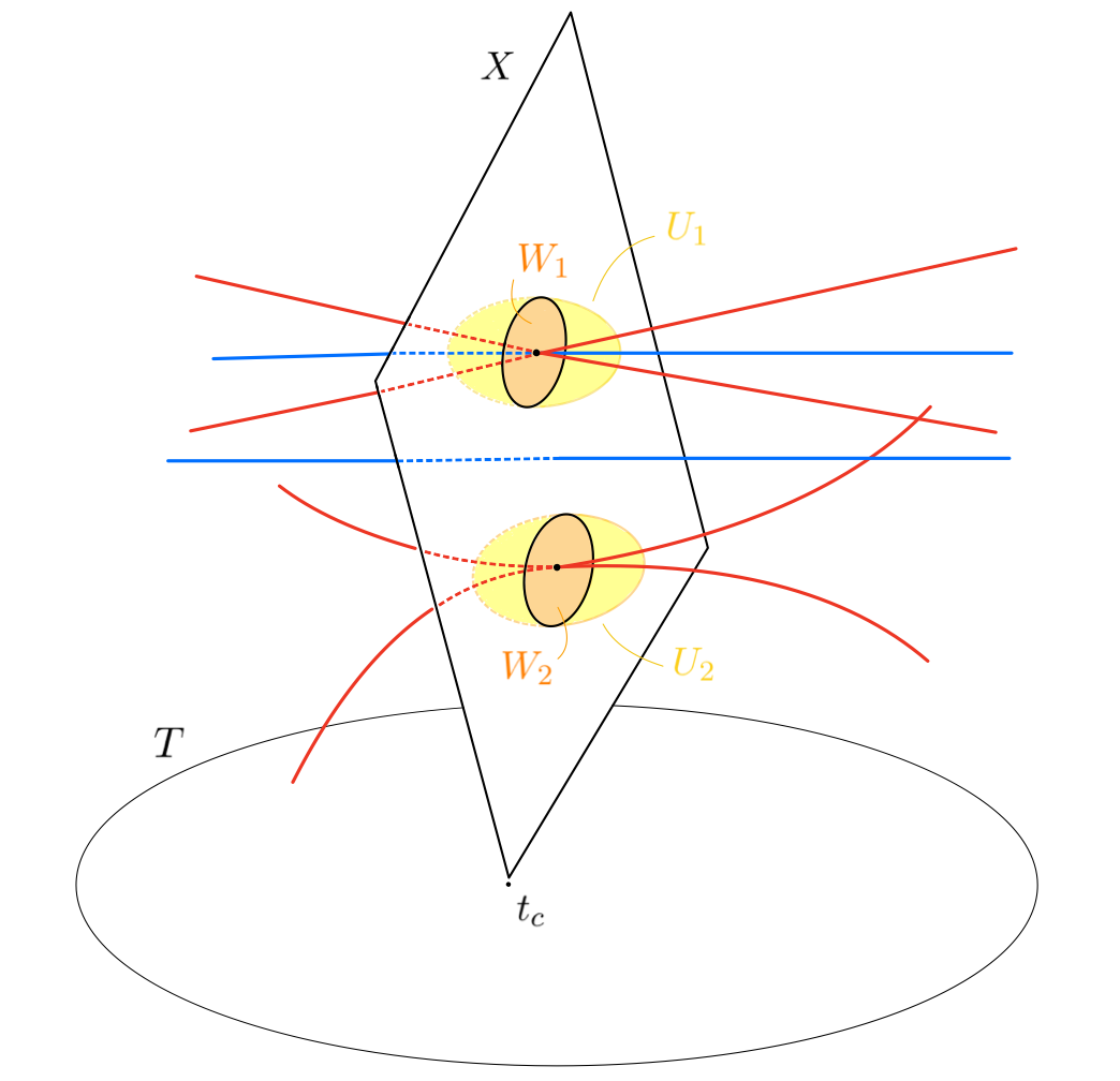
Figure 10. Global and fibrewise localization.

Consider now the corresponding open balls $W_{p}=y_{p}^{-1}(W\times\{0\})\subset Y_{t_{c}}$ in the fibre over $t_{c}$. Observe that the unit sphere $\partial W=\mathbb{S}^{2n-1}$ lies transverse to the arrangement (3.7). It follows that the closure of the disjoint union

$$W_{P}\mathrel{\mathop{:}}=\bigsqcup_{p\in P}W_{p}\;\subset\;Y_{t_{c}}$$

embeds as a compact submanifold, whose boundary intersects $\mathfrak{D}$ transversely. Furthermore, $W_{P}\supset P$ contains all critical points over $t_{c}$. In fact, since $P$ is finite and the simple pinches ($\sharp$ ‣ 3.3) depend continuously on $t$, we conclude that every local trivialization $\pi^{-1}(V)\cong X\times V$ of $Y$ at $t_{c}\in V\subseteq T$ can be restricted to an open $V^{\prime}\subseteq V$, still containing $t_{c}$, such that $W_{P}\times V^{\prime}$ contains all critical points over $V^{\prime}$ (fig. 10).

Corollary 3.15.

Let $t_{c}\in L$ a simple critical value, and $[\gamma]\in\pi_{1}(T\setminus L,t_{0})$ a class that can be represented by a small loop near $t_{c}$. Then the variation along $\gamma$ decomposes into a sum

(3.8) $$\operatorname{Var}_{\gamma}=\sum_{p\in P}\operatorname{Var}_{p}\quad\text{where}\quad\operatorname{Var}_{p}=\iota_{p*}\operatorname{var}_{p}W_{p*}.$$

Proof.

Apply 3.7 to $W_{P}$ to find an ambient isotopy $g_{\gamma}$ of $D_{t_{0}}$ inside $X$, so that $g_{\gamma}$ is the identity outside $W_{P}$. By continuity, $g_{\gamma}(W_{p})=W_{p}$ maps each ball to itself. Therefore, in the splitting

from the disjoint union $\overline{W_{P}}=\bigsqcup_{p}\overline{W_{p}}$, the map $\operatorname{var}_{\gamma}$ from 3.11, viewed as a matrix (arrow on the left), is diagonal: $\operatorname{var}_{\gamma}=\bigoplus_{p}\operatorname{var}_{p}$. The entry $\operatorname{var}_{p}$ is the restriction of $\operatorname{id}-g_{\gamma*}$ to $W_{p}$ and thus equal to the factorization of the variation $\operatorname{Var}_{p}=\operatorname{id}-g_{p*}$ induced by the homeomorphism $g_{p}\colon X\rightarrow X$ defined by $g_{p}(x)=g_{\gamma}(x)$ for $x\in W_{p}$ and $g_{p}(x)=x$ otherwise. ∎

For a simple pinch $p\in cS$ on a stratum $S$ of codimension $m$, let $J\subseteq\mathfrak{A}$ and $K\subseteq\mathfrak{B}$ denote the $m=\lvert J\rvert+\lvert K\rvert$ hypersurfaces in $A$ and $B$, respectively, that contain the pinch: $p\in D^{J\sqcup K}$. We chose $W_{p}$ so small that the pairs

$$(W_{p}\setminus A,B) =(W_{p}\setminus A_{J},B_{K})\quad\text{and}$$

$$(\overline{W_{p}}\setminus A,\partial W_{p}\cup B) =(\overline{W_{p}}\setminus A_{J},\partial W_{p}\cup B_{K})$$

only meet precisely those hypersurfaces. We have thus reduced the computation of the variation $\operatorname{Var}_{\gamma}$, at least for small loops around Landau singularities $\ell\subseteq L$ with a simple critical value $t_{c}\in\ell$, to a calculation of $\operatorname{var}_{p}$ for the arrangement (3.7) within the unit ball $W\subset\mathbb{C}^{n}$. The coordinates $y_{p}$ translate $J\sqcup K$ into a bipartition of $\{S_{1},\ldots,S_{m}\}$.

3.4. Leray’s residue and (co)boundary maps

To state the relative Picard-Lefschetz theorem, we employ two operations on relative homology groups: the partial boundary $\partial_{i}$ and the relative coboundary $\delta_{i}$. These were constructed by Leray in [39] and a review is provided in appendix B.

In summary, we assume that $\mathfrak{D}=(D_{1},D_{2},\ldots)$ is a finite transverse family of smooth complex hypersurfaces $D_{i}\subset X$ inside a complex manifold $X$. For any index set $I$, we denote the corresponding union and intersection by

$$D_{I}=\bigcup_{i\in I}D_{i}\qquad\text{and}\qquad D^{I}=\bigcap_{i\in I}D_{i}.$$

Then for disjoint index sets $I\cap J=\varnothing$, and any $i\in J$, Leray’s partial boundary comes from the usual boundary map in relative homology, but only keeps the piece that lies in $D_{i}\subseteq D_{J}$. This partial boundary is denoted

$$\partial_{i}\colon H_{\bullet}(X\setminus D_{I},D_{J})\longrightarrow H_{\bullet-1}(D_{i}\setminus D_{I},D_{J-i})$$

and it fits into a long exact sequence of the form

(3.9) $$\cdots\rightarrow H_{\bullet}(X\setminus D_{I},D_{J-i})\rightarrow H_{\bullet}(X\setminus D_{I},D_{J})\xrightarrow{\partial_{i}}H_{\bullet-1}(D_{i}\setminus D_{I},D_{J-i})\rightarrow\cdots$$

where the other two maps are the natural inclusions of pairs.

Leray’s relative coboundary takes a chain in $D_{i}$ (for some $i\in I$) and fibres it in circles through a tubular neighbourhood around $D_{i}$. This yields a homomorphism

$$\delta_{i}\colon H_{\bullet}(D_{i}\setminus D_{I-i},D_{J})\longrightarrow H_{\bullet+1}(X\setminus D_{I},D_{J})$$

which also fits into a long exact sequence

$$\cdots\rightarrow H_{\bullet}(X\setminus D_{I-i},D_{J})\xrightarrow{\varpi_{i}}H_{\bullet-2}(D_{i}\setminus D_{I-i},D_{J})\xrightarrow{\delta_{i}}H_{\bullet-1}(X\setminus D_{I},D_{J})\rightarrow\cdots$$

where the map $\varpi_{i}$ intersects a transverse chain with $D_{i}$. For multiple indices $K=\{i_{1},\ldots,i_{r}\}\subseteq J$, we denote the corresponding iterated boundaries and coboundaries as

$$\partial_{K} =\partial_{i_{1}}\!\cdots\partial_{i_{r}}\colon H_{\bullet}(X\setminus D_{I},D_{J})\longrightarrow H_{\bullet-r}(D^{K}\setminus D_{I},D_{J-K})\quad\text{and}$$

$$\delta_{K} =\delta_{i_{1}}\!\cdots\delta_{i_{r}}\colon H_{\bullet}(D^{K}\setminus D_{I},D_{J-K})\longrightarrow H_{\bullet+r}(X\setminus D_{I+K},D_{J-K}).$$

The ordering of these compositions only affects the overall sign, since for $i\neq j$, the maps $\partial_{i}\partial_{j}=-\partial_{j}\partial_{i}$ and $\delta_{i}\delta_{j}=-\delta_{j}\delta_{i}$ and $\partial_{i}\delta_{j}=-\delta_{j}\partial_{i}$ anticommute.

Remark 3.16.

On the level of differential forms (de Rham cohomology), the Leray coboundary is dual to Leray’s residue map

$$\operatorname{Res}_{i}\colon H^{\bullet}_{\mathsf{dR}}(X\setminus D_{I},D_{J})\longrightarrow H_{\mathsf{dR}}^{\bullet-1}(D_{i}\setminus D_{I-i},D_{J}).$$

The latter generalizes the Cauchy residue of a function: for any chain $\sigma$ in $D_{i}\setminus D_{I-i}$ with boundary in $D_{J}$, and any closed smooth form $\omega\in\Omega^{\bullet}(X\setminus D_{I})$ that vanishes on $D_{J}$, their (co)homology classes $[\sigma]$ and $[\omega]$ integrate to

(3.10) $$\int_{\delta_{i}[\sigma]}[\omega]=2\mathrm{i}\pi\cdot\int_{[\sigma]}\operatorname{Res}_{i}[\omega].$$

3.5. Vanishing chains

The Picard-Lefschetz theorem describes the variation $\operatorname{Var}_{p}$ at a linear or quadratic simple pinch, in terms of certain homology classes of the arrangement (3.7). The example in section 1.8.1 illustrates these classes in dimension $n=1$; illuminating figures for higher dimensions can be found in [51, Fig. V.2] and [61, Figs. I.14–16].

From now on we employ the localization discussed in the context of small and simple loops (3.1), that is, we assume $T=\mathbb{C}$ and $\ell=\{0\}$.

Definition 3.17.

Let $p\in cS$ denote a linear or quadratic simple pinch on a stratum $S\subseteq A^{J}\cap B^{K}$ of codimension $m$. Let $A_{j}\in\mathfrak{A}$ ($j\in J$) and $B_{k}\in\mathfrak{B}$ ($k\in K$) denote the hypersurfaces containing $S$. Recall that, in coordinates of the form (3.7), these define a bipartition $J\sqcup K=\{1,\ldots,m\}$. Let $0<t<1$.

1. The vanishing cell $\zeta\in H_{n}(W_{p},A\cup B)_{t}\cong H_{n}(W,S_{1,\ldots,m})_{t}$ is the class of the compact region in real coordinates $x\in\mathbb{R}^{n}$, bounded by all $m$ hypersurfaces $S_{i}$, in the fibre over $t$:

   $$\quad\quad\quad\{x_{1},\ldots,x_{m-1}\geq 0\}\cap\{x_{m}^{2}+\ldots+x_{n}^{2}\leq t-x_{1}-\ldots-x_{m-1}\}\subset\mathbb{R}^{n}.$$

2. The vanishing cycle $\nu\in H_{n}(W_{p}\setminus A,B)_{t}\cong H_{n}(W\setminus S_{J},S_{K})_{t}$ is obtained from the vanishing cell by taking first the boundary in, and then the Leray coboundary around, each hypersurface $A_{j}$:

   (3.11) $$\nu=\Big{(}\prod_{j\in J}\delta_{A_{j}}\partial_{A_{j}}\Big{)}\>\zeta.$$

3. The dual vanishing cycle $\widetilde{\nu}\in H_{n}(W_{p}\setminus B,A)_{t}\cong H_{n}(W\setminus S_{K},S_{J})_{t}$ is obtained in the same way, but swapping the roles of $A$ and $B$:

   $$\widetilde{\nu}=(-1)^{\lvert K\rvert}\cdot\Big{(}\prod_{k\in K}\delta_{B_{k}}\partial_{B_{k}}\Big{)}\>\zeta.$$

4. Their images under the inclusion $\iota_{p}\colon W_{p}\hookrightarrow Y_{t}$ are denoted

   $$\quad\quad\quad\quad\quad\nu_{p}=\iota_{p*}\nu\in H_{n}(Y\setminus A,B)_{t}\quad\text{and}\quad\widetilde{\nu}_{p}=\iota_{p*}\widetilde{\nu}\in H_{n}(Y\setminus B,A)_{t}.$$

Remark 3.18.

The operators $\delta_{j}\partial_{j}$ in (3.11) are even, hence $\nu$ and $\widetilde{\nu}$ depend only on the orientation of $\zeta$, but not on any implicit ordering of $J$ or $K$. In fact, for any ordering $J=\{j_{1},\ldots,j_{r}\}$, we have $\nu=(-1)^{\lvert J\rvert(\lvert J\rvert-1)/2}\cdot\delta_{J}\partial_{J}\zeta$ in terms of $\delta_{J}=\delta_{j_{1}}\!\cdots\delta_{j_{r}}$ and $\partial_{J}=\partial_{j_{1}}\!\cdots\partial_{j_{r}}$.

The vanishing cell $\zeta$ varies continuously with $t\in(0,1)$ and it literally vanishes as $t\rightarrow 0$; hence the name. For a linear pinch ($m=n+1$), $\zeta$ is the simplex bounded by $x_{i}\geq 0$ (from $S_{i}$ for $i\leq n$) and $x_{1}+\ldots+x_{n}\leq t$ from

$$S_{n+1}=\{x_{1}+\ldots+x_{n}=t\}.$$

For a quadratic pinch ($m\leq n$), $\zeta$ is a family of $n-m+1$ dimensional disks (coordinates $x_{m},\ldots,x_{n}$) over an $m-1$ dimensional simplex $\{x_{1}+\ldots+x_{m-1}\leq t,x_{i}\geq 0\}$, with the disks collapsing to a point over $x_{1}+\ldots+x_{m-1}=t$. The maximal boundary of this cell,

$$\partial_{1,\ldots,m}\zeta=\pm[\mathbb{S}^{n-m}]\in H_{n-m}(W\cap S^{1,\ldots,m}_{t}),$$

is the fundamental class of the vanishing sphere. This name refers to the embedded spheres $\mathbb{S}^{n-m}\hookrightarrow S^{1,\ldots,m}_{t}\subset\mathbb{C}^{n}$, $u\mapsto(0,\ldots,0,u\cdot\sqrt{t})$. See [51, Fig. V.2] and [61, Figs. I.14–16] for figures of these vanishing chains for $n\leq 3$ and $m\leq 4$.

Remark 3.19.

We treat the zero-dimensional sphere $\mathbb{S}^{0}=\{1,-1\}\subseteq\mathbb{R}$ as an oriented manifold with the orientation induced from the interval $(-1,1)\subseteq\mathbb{R}$. So its fundamental class is $[\mathbb{S}^{0}]=[\{1\}]-[\{-1\}]\in H_{0}(\mathbb{S}^{0})$.

The vanishing cell $\zeta$ is defined only up to a sign (orientation). There is no canonical choice, because the natural orientations on $\mathbb{R}^{n}$ are not compatible between different parametrizations (3.7); e.g. swap $x_{1}\leftrightarrow x_{2}$. This sign is the only ambiguity, because the vanishing cell is a generator of the cyclic group

$$\zeta \in H_{n}(W_{p},A\cup B)_{t}\cong\mathbb{Z}.$$

This isomorphism is reviewed in 3.29. The (dual) vanishing cycles $\nu$ and $\widetilde{\nu}$ also depend on the orientation of $\zeta$, but nothing more (3.18). Hence the sign ambiguity cancels in the quadratic expression $\langle{\widetilde{\nu}}\,|\,{h}\rangle\cdot\nu$ in the Picard-Lefschetz formula.

Lemma 3.20.

The monodromy of the vanishing cell of a simple pinch, along a simple loop $\gamma(\tau)=t\cdot e^{2\mathrm{i}\pi\tau}$ based at $t\in(0,1)$, is

$$\gamma_{*}\zeta=(-1)^{n-m+1}\cdot\zeta.$$

Proof.

The trivialization $\phi_{\tau}(x)=(x_{1}e^{2\mathrm{i}\pi\tau},\ldots,x_{m-1}e^{2\mathrm{i}\pi\tau},x_{m}e^{\mathrm{i}\pi\tau},\ldots,x_{n}e^{\mathrm{i}\pi\tau})$ identifies the fibres over $\gamma$. It lifts the vanishing cell to a section $\phi_{\tau*}(\zeta)\in H_{n}(W,S_{1,\ldots,m})_{\gamma(\tau)}$. After one revolution, $\phi_{1*}$ acts by $(-1)^{n-m+1}$ on the orientation $\mathrm{d}x_{1}\wedge\ldots\wedge\mathrm{d}x_{n}$, because $\phi_{1}(x)=(x_{1},\ldots,x_{m-1},-x_{m},\ldots,-x_{n})$. ∎

This simple computation determines the variation of the vanishing cycles, because variation commutes with (co)boundary maps:

(3.12) $$\operatorname{Var}_{\gamma}\nu_{p}=\left[(-1)^{n-m+1}-1\right]\cdot\nu_{p}=\begin{cases}0&\text{if $n-m$ odd, and}\\ -2\nu_{p}&\text{if $n-m$ even.}\\ \end{cases}$$

Beware this does not imply that $\operatorname{Var}_{\gamma}=0$ for $n-m$ odd. Consider the map of pairs $(W_{p}\setminus A,B)\rightarrow(\overline{W}_{p}\setminus A,\partial W_{p}\cup B)$, which induces

(3.13) $$W_{*}\iota_{*}\colon H_{n}(W_{p}\setminus A,B)\longrightarrow H_{n}(\overline{W}_{p}\setminus A,\partial W_{p}\cup B).$$

We will see later that, for odd $n-m\geq 1$, this map is zero. Hence $\operatorname{Var}_{\gamma}\nu_{p}=0$ simply reflects the fact that the $W$-trace of $\nu_{p}$ is zero; we learn nothing about $\operatorname{var}_{p}$ in (3.8). The linear pinch $n-m=-1$ is more subtle.

3.6. Picard-Lefschetz theorem

Several variants of the Picard-Lefschetz theorem can be found for example in [21, 35, 34]. The following relative version for hypersurface arrangements $D=A\cup B$ is stated in [51], albeit without a complete proof, and with an inaccurate interpretation for linear pinches.

Theorem 3.21.

Let $p\in D$ be a linear or quadratic simple pinch over a smooth point $\pi(p)\in L$ of the Landau variety. Then the local variation

$$\operatorname{var}_{p}\colon H_{d}(\overline{W}_{p}\setminus A,\partial W_{p}\cup B)_{t}\longrightarrow H_{d}(W_{p}\setminus A,B)_{t}$$

can be expressed in terms of the vanishing cycles $\nu\in H_{n}(W_{p}\setminus A,B)_{t}$ and $\widetilde{\nu}\in H_{n}(W_{p}\setminus B,A)_{t}$ from 3.17:

• In degree $d\neq n$, $\operatorname{var}_{p}=0$.

• In degree $d=n$, there exist integers $N(h)\in\mathbb{Z}$ such that

  (3.14) $$\operatorname{var}_{p}(h)=N(h)\cdot\nu.$$

• This identity holds for the intersection numbers

  (3.15) $$N(h)=(-1)^{(n+1)(n+2)/2}\cdot\langle{\widetilde{\nu}}\,|\,{h}\rangle.$$

Remark 3.22.

The theorem covers linear and quadratic pinches simultaneously, but they behave slightly differently. At a quadratic pinch, the variation map $\operatorname{var}_{p}$ is always non-zero. At a linear pinch $p$, we distinguish three cases:

• If $p\in A\setminus B$ (“$A$ type”), then $\nu_{p}=0$ and thus $\operatorname{var}_{p}=0$.

• If $p\in B\setminus A$ (“$B$ type”), then $\widetilde{\nu}_{p}=0$ and thus $\operatorname{var}_{p}=0$.

• If $p\in A\cap B$ (“mixed type”), then $\operatorname{var}_{p}\neq 0$.

At an $A$-type linear pinch, (3.14) holds for any choice of $N(h)$. For all other simple pinches, the integer $N(h)$ in (3.15) is the unique solution to (3.14).

For a trace $h=W_{p*}\,\sigma$ of some cycle $\sigma\in H_{n}(Y\setminus A,B)_{t}$, the intersection (3.15) inside the ball $W_{p}$ can also be thought of as taking place in the fibre $Y_{t}$,

$$\langle{\widetilde{\nu}}\,|\,{W_{p*}\,\sigma}\rangle=\langle{\widetilde{\nu}_{p}}\,|\,{\sigma}\rangle,$$

because $\partial W_{p}$ is transverse to $D$. The local formulas globalize with (3.8):

Corollary 3.23.

For a small loop $\gamma$ around a simple pinch component $\ell\in\mathfrak{L}$, the variation $\operatorname{Var}_{\gamma}$ on $H_{n}(Y\setminus A,B)_{t}$ can be written as:

(3.16) $$\operatorname{Var}_{\gamma}(\sigma)=(-1)^{(n+1)(n+2)/2}\cdot\sum_{p}\langle{\widetilde{\nu}_{p}}\,|\,{\sigma}\rangle\cdot\nu_{p}.$$

Remark 3.24.

Let $A_{j}$ ($j\in J$) and $B_{k}$ ($k\in K$) denote the hypersurfaces that contain the pinch $p$. Iterating $\langle{\delta\widetilde{\nu}}\,|\,{h}\rangle=(-1)^{d}\langle{\widetilde{\nu}}\,|\,{\partial h}\rangle$ from (C.4), with $d$ the degree of $h$, the intersection number reduces to

$$\langle{\widetilde{\nu}}\,|\,{h}\rangle=(-1)^{n\lvert K\rvert+\lvert K\rvert(\lvert K\rvert+1)/2}\cdot\langle{\partial_{K}\zeta}\,|\,{\partial_{K}h}\rangle.$$

The coefficient $N(h)$ can thus be computed on the manifold $\overline{M}=\overline{W_{p}}\cap B^{K}$ with its intersection pairing $H_{n-\lvert K\rvert}(M,A^{\prime})\times H_{n-\lvert K\rvert}(\overline{M}\setminus A^{\prime},\partial M)\rightarrow\mathbb{Z}$ for $A^{\prime}=B^{K}\cap A_{J}$, after taking all $B_{k}$-boundaries of $\zeta$ and $h$.

For the proof of 3.21, we fix a pinch $p$ (henceforth suppressing the subscript _p) and consider every disjoint triple $I\sqcup J\sqcup K\subseteq\{1,\ldots,m\}$ of the hypersurfaces $S_{1},\ldots,S_{m}\subset\mathbb{C}^{n}$ that contain $p$, as in (3.7). The corresponding divisors $S_{J}\cap S^{I}\cap W$ and $S_{K}\cap S^{I}\cap W$ inside the manifold $W\cap S^{I}\subset\mathbb{C}^{n}$ define pairs of fibre bundles with associated variations

(3.17) $$\operatorname{var}\colon H_{\bullet}(\overline{W}\cap S^{I}\setminus S_{J},\partial W\cup S_{K})_{t}\longrightarrow H_{\bullet}(W\cap S^{I}\setminus S_{J},S_{K})_{t}.$$

Remark 3.25.

The configuration of a strict subset $I\sqcup J\sqcup K\subset\{1,\ldots,m\}$ has no critical points and thus $\operatorname{var}=0$. Henceforth, we consider only the case of tripartitions $I\sqcup J\sqcup K=\{1,\ldots,m\}$ of all $m$ hypersurfaces.

More precisely, we define the variations (3.17) by choosing a single isotopy $g_{\gamma}$ as in 3.7. We then obtain $\operatorname{var}=g^{\prime}_{*}-\operatorname{id}$ via 3.11, using the corresponding restrictions $g^{\prime}=g_{\gamma}|_{S^{I}\setminus S_{J}}$ of $g_{\gamma}$. Thus all variations arise from the same isotopy, and no confusion should arise from denoting all of them with the same symbol $\operatorname{var}$.

Furthermore, since (co)boundaries commute with push-forward, see (B.6), the following diagram commutes for all $i\in I$:

(3.18) $$\begin{gathered}\lx@xy@svg{\hbox{\raise 0.0pt\hbox{\kern 63.44283pt\hbox{\ignorespaces\ignorespaces\ignorespaces\hbox{\vtop{\kern 0.0pt\offinterlineskip\halign{\entry@#!@&&\entry@@#!@\cr&\\&\\&\\}}}\ignorespaces{\hbox{\kern-63.44283pt\raise 0.0pt\hbox{\hbox{\kern 0.0pt\raise 0.0pt\hbox{\hbox{\kern 3.0pt\raise 0.0pt\hbox{$\textstyle{H_{\bullet}(\overline{W}\cap S^{I-i}\setminus S_{J},\partial W\cup S_{K+i})_{t}\ignorespaces\ignorespaces\ignorespaces\ignorespaces\ignorespaces\ignorespaces\ignorespaces\ignorespaces}$}}}}}}}\ignorespaces\ignorespaces\ignorespaces\ignorespaces{}{\hbox{\lx@xy@droprule}}\ignorespaces\ignorespaces\ignorespaces{\hbox{\kern 72.74084pt\raise 4.50694pt\hbox{{}\hbox{\kern 0.0pt\raise 0.0pt\hbox{\hbox{\kern 3.0pt\hbox{\hbox{\kern 0.0pt\raise-1.50694pt\hbox{$\scriptstyle{\operatorname{var}}$}}}\kern 3.0pt}}}}}}\ignorespaces{\hbox{\kern 97.58612pt\raise 0.0pt\hbox{\hbox{\kern 0.0pt\raise 0.0pt\hbox{\lx@xy@tip{1}\lx@xy@tip{-1}}}}}}{\hbox{\lx@xy@droprule}}{\hbox{\lx@xy@droprule}}\ignorespaces\ignorespaces\ignorespaces\ignorespaces{}{\hbox{\lx@xy@droprule}}\ignorespaces\ignorespaces\ignorespaces{\hbox{\kern 0.0pt\raise-20.62332pt\hbox{{}\hbox{\kern 0.0pt\raise 0.0pt\hbox{\hbox{\kern 3.0pt\hbox{\hbox{\kern 0.0pt\raise-1.77103pt\hbox{$\scriptstyle{\partial_{i}}$}}}\kern 3.0pt}}}}}}\ignorespaces{\hbox{\kern 0.0pt\raise-29.5pt\hbox{\hbox{\kern 0.0pt\raise 0.0pt\hbox{\lx@xy@tip{1}\lx@xy@tip{-1}}}}}}{\hbox{\lx@xy@droprule}}{\hbox{\lx@xy@droprule}}{\hbox{\kern 97.58612pt\raise 0.0pt\hbox{\hbox{\kern 0.0pt\raise 0.0pt\hbox{\hbox{\kern 3.0pt\raise 0.0pt\hbox{$\textstyle{H_{\bullet}(W\cap S^{I-i}\setminus S_{J},S_{K+i})_{t}\ignorespaces\ignorespaces\ignorespaces\ignorespaces}$}}}}}}}\ignorespaces\ignorespaces\ignorespaces\ignorespaces{}{\hbox{\lx@xy@droprule}}\ignorespaces\ignorespaces\ignorespaces{\hbox{\kern 150.59668pt\raise-20.62332pt\hbox{{}\hbox{\kern 0.0pt\raise 0.0pt\hbox{\hbox{\kern 3.0pt\hbox{\hbox{\kern 0.0pt\raise-1.77103pt\hbox{$\scriptstyle{\partial_{i}}$}}}\kern 3.0pt}}}}}}\ignorespaces{\hbox{\kern 150.59668pt\raise-29.5pt\hbox{\hbox{\kern 0.0pt\raise 0.0pt\hbox{\lx@xy@tip{1}\lx@xy@tip{-1}}}}}}{\hbox{\lx@xy@droprule}}{\hbox{\lx@xy@droprule}}{\hbox{\kern-60.73576pt\raise-41.24664pt\hbox{\hbox{\kern 0.0pt\raise 0.0pt\hbox{\hbox{\kern 3.0pt\raise 0.0pt\hbox{$\textstyle{H_{\bullet-1}(\overline{W}\cap S^{I}\setminus S_{J},\partial W\cup S_{K})_{t}\ignorespaces\ignorespaces\ignorespaces\ignorespaces\ignorespaces\ignorespaces\ignorespaces\ignorespaces}$}}}}}}}\ignorespaces\ignorespaces\ignorespaces\ignorespaces{}{\hbox{\lx@xy@droprule}}\ignorespaces\ignorespaces\ignorespaces{\hbox{\kern 72.74084pt\raise-36.7397pt\hbox{{}\hbox{\kern 0.0pt\raise 0.0pt\hbox{\hbox{\kern 3.0pt\hbox{\hbox{\kern 0.0pt\raise-1.50694pt\hbox{$\scriptstyle{\operatorname{var}}$}}}\kern 3.0pt}}}}}}\ignorespaces{\hbox{\kern 100.29318pt\raise-41.24664pt\hbox{\hbox{\kern 0.0pt\raise 0.0pt\hbox{\lx@xy@tip{1}\lx@xy@tip{-1}}}}}}{\hbox{\lx@xy@droprule}}{\hbox{\lx@xy@droprule}}\ignorespaces\ignorespaces\ignorespaces\ignorespaces{}{\hbox{\lx@xy@droprule}}\ignorespaces\ignorespaces\ignorespaces{\hbox{\kern 0.0pt\raise-61.86996pt\hbox{{}\hbox{\kern 0.0pt\raise 0.0pt\hbox{\hbox{\kern 3.0pt\hbox{\hbox{\kern 0.0pt\raise-1.77103pt\hbox{$\scriptstyle{\delta_{i}}$}}}\kern 3.0pt}}}}}}\ignorespaces{\hbox{\kern 0.0pt\raise-70.74664pt\hbox{\hbox{\kern 0.0pt\raise 0.0pt\hbox{\lx@xy@tip{1}\lx@xy@tip{-1}}}}}}{\hbox{\lx@xy@droprule}}{\hbox{\lx@xy@droprule}}{\hbox{\kern 100.29318pt\raise-41.24664pt\hbox{\hbox{\kern 0.0pt\raise 0.0pt\hbox{\hbox{\kern 3.0pt\raise 0.0pt\hbox{$\textstyle{H_{\bullet-1}(W\cap S^{I}\setminus S_{J},S_{K})_{t}\ignorespaces\ignorespaces\ignorespaces\ignorespaces}$}}}}}}}\ignorespaces\ignorespaces\ignorespaces\ignorespaces{}{\hbox{\lx@xy@droprule}}\ignorespaces\ignorespaces\ignorespaces{\hbox{\kern 150.59668pt\raise-61.86996pt\hbox{{}\hbox{\kern 0.0pt\raise 0.0pt\hbox{\hbox{\kern 3.0pt\hbox{\hbox{\kern 0.0pt\raise-1.77103pt\hbox{$\scriptstyle{\delta_{i}}$}}}\kern 3.0pt}}}}}}\ignorespaces{\hbox{\kern 150.59668pt\raise-70.74664pt\hbox{\hbox{\kern 0.0pt\raise 0.0pt\hbox{\lx@xy@tip{1}\lx@xy@tip{-1}}}}}}{\hbox{\lx@xy@droprule}}{\hbox{\lx@xy@droprule}}{\hbox{\kern-63.44283pt\raise-82.49329pt\hbox{\hbox{\kern 0.0pt\raise 0.0pt\hbox{\hbox{\kern 3.0pt\raise 0.0pt\hbox{$\textstyle{H_{\bullet}(\overline{W}\cap S^{I-i}\setminus S_{J+i},\partial W\cup S_{K})_{t}\ignorespaces\ignorespaces\ignorespaces\ignorespaces}$}}}}}}}\ignorespaces\ignorespaces\ignorespaces\ignorespaces{}{\hbox{\lx@xy@droprule}}\ignorespaces\ignorespaces\ignorespaces{\hbox{\kern 73.36308pt\raise-77.98634pt\hbox{{}\hbox{\kern 0.0pt\raise 0.0pt\hbox{\hbox{\kern 3.0pt\hbox{\hbox{\kern 0.0pt\raise-1.50694pt\hbox{$\scriptstyle{\operatorname{var}}$}}}\kern 3.0pt}}}}}}\ignorespaces{\hbox{\kern 98.83058pt\raise-82.49329pt\hbox{\hbox{\kern 0.0pt\raise 0.0pt\hbox{\lx@xy@tip{1}\lx@xy@tip{-1}}}}}}{\hbox{\lx@xy@droprule}}{\hbox{\lx@xy@droprule}}{\hbox{\kern 98.83058pt\raise-82.49329pt\hbox{\hbox{\kern 0.0pt\raise 0.0pt\hbox{\hbox{\kern 3.0pt\raise 0.0pt\hbox{$\textstyle{H_{\bullet}(W\cap S^{I-i}\setminus S_{J-i},S_{K})_{t}}$}}}}}}}\ignorespaces}}}}\ignorespaces\end{gathered} \textstyle{H_{\bullet}(\overline{W}\cap S^{I-i}\setminus S_{J},\partial W\cup S_{K+i})_{t}\ignorespaces\ignorespaces\ignorespaces\ignorespaces\ignorespaces\ignorespaces\ignorespaces\ignorespaces} \scriptstyle{\operatorname{var}} \scriptstyle{\partial_{i}} \textstyle{H_{\bullet}(W\cap S^{I-i}\setminus S_{J},S_{K+i})_{t}\ignorespaces\ignorespaces\ignorespaces\ignorespaces} \scriptstyle{\partial_{i}} \textstyle{H_{\bullet-1}(\overline{W}\cap S^{I}\setminus S_{J},\partial W\cup S_{K})_{t}\ignorespaces\ignorespaces\ignorespaces\ignorespaces\ignorespaces\ignorespaces\ignorespaces\ignorespaces} \scriptstyle{\operatorname{var}} \scriptstyle{\delta_{i}} \textstyle{H_{\bullet-1}(W\cap S^{I}\setminus S_{J},S_{K})_{t}\ignorespaces\ignorespaces\ignorespaces\ignorespaces} \scriptstyle{\delta_{i}} \textstyle{H_{\bullet}(\overline{W}\cap S^{I-i}\setminus S_{J+i},\partial W\cup S_{K})_{t}\ignorespaces\ignorespaces\ignorespaces\ignorespaces} \scriptstyle{\operatorname{var}} \textstyle{H_{\bullet}(W\cap S^{I-i}\setminus S_{J-i},S_{K})_{t}} \textstyle{H_{\bullet}(\overline{W}\cap S^{I-i}\setminus S_{J},\partial W\cup S_{K+i})_{t}\ignorespaces\ignorespaces\ignorespaces\ignorespaces\ignorespaces\ignorespaces\ignorespaces\ignorespaces} \scriptstyle{\operatorname{var}} \scriptstyle{\partial_{i}} \textstyle{H_{\bullet}(W\cap S^{I-i}\setminus S_{J},S_{K+i})_{t}\ignorespaces\ignorespaces\ignorespaces\ignorespaces} \scriptstyle{\partial_{i}} \textstyle{H_{\bullet-1}(\overline{W}\cap S^{I}\setminus S_{J},\partial W\cup S_{K})_{t}\ignorespaces\ignorespaces\ignorespaces\ignorespaces\ignorespaces\ignorespaces\ignorespaces\ignorespaces} \scriptstyle{\operatorname{var}} \scriptstyle{\delta_{i}} \textstyle{H_{\bullet-1}(W\cap S^{I}\setminus S_{J},S_{K})_{t}\ignorespaces\ignorespaces\ignorespaces\ignorespaces} \scriptstyle{\delta_{i}} \textstyle{H_{\bullet}(\overline{W}\cap S^{I-i}\setminus S_{J+i},\partial W\cup S_{K})_{t}\ignorespaces\ignorespaces\ignorespaces\ignorespaces} \scriptstyle{\operatorname{var}} \textstyle{H_{\bullet}(W\cap S^{I-i}\setminus S_{J-i},S_{K})_{t}}$$

Following [21], the strategy to prove 3.21 is to exploit these diagrams to reduce the calculation to a few special cases. For a quadratic pinch, we can always reduce to $J=K=\varnothing$ (section 3.8). For a linear pinch (section 3.7), we have to distinguish three different types, as in 3.22.

To spell out these reductions, we extend 3.17 and denote, for all $I\sqcup J\sqcup K=\{1,\ldots,m\}$, the respective (dual) vanishing cycles as

$$\nu =\Big{(}\prod_{j\in J}\delta_{j}\partial_{j}\Big{)}\partial_{I}\zeta \in H_{n-\lvert I\rvert}(W\cap S^{I}\setminus S_{J},S_{K})\quad\text{and}$$

$$\widetilde{\nu} =(-1)^{\lvert K\rvert}\cdot\Big{(}\prod_{k\in K}\delta_{k}\partial_{k}\Big{)}\partial_{I}\zeta \in H_{n-\lvert I\rvert}(W\cap S^{I}\setminus S_{K},S_{J}).$$

Then 3.21 arises as the special case $I=\varnothing$ of

Theorem 3.26.

For every tripartition $(I,J,K)$, the variation (3.17) is zero in all degrees other than $n-\lvert I\rvert$. For a class $h$ in degree $n-\lvert I\rvert$,

(3.19) $$\operatorname{var}h=(-1)^{(n-\lvert I\rvert+1)(n-\lvert I\rvert+2)/2}\cdot\langle{\widetilde{\nu}}\,|\,{h}\rangle\cdot\nu.$$

Note that, for this formula to make any sense, it has to be compatible with the commutative diagram (3.18). This can be verified easily:

Lemma 3.27.

Let $\operatorname{\widetilde{\operatorname{var}}}\colon H_{\bullet}(\overline{W}\cap S^{I}\setminus S_{J},\partial W\cup S_{K})_{t}\longrightarrow H_{\bullet}(W\cap S^{I}\setminus S_{J},S_{K})_{t}$ denote the map defined by the right-hand side of (3.19). Then the diagram (3.18), with $\operatorname{\widetilde{\operatorname{var}}}$ in place of $\operatorname{var}$, is commutative.

Proof.

Consider the bottom square of (3.18), relating the variations of the triples $(I,J,K)$ and $(I^{\prime},J^{\prime},K^{\prime})=(I-i,J+i,K)$. Let $\nu^{\prime}$ and $\widetilde{\nu}^{\prime}$ denote the vanishing cycles for $(I^{\prime},J^{\prime},K^{\prime})$. Note that $\nu^{\prime}=\epsilon\delta_{i}\nu$ and $\widetilde{\nu}=\epsilon\partial_{i}\widetilde{\nu}^{\prime}$, where the sign $\epsilon=\pm 1$ is determined by the order of $I$ such that $\partial_{I}=\epsilon\partial_{i}\partial_{I-i}$. Thus,

$$\delta_{i}(\operatorname{\widetilde{\operatorname{var}}}h) =(-1)^{(d+1)(d+2)/2}\cdot\langle{\widetilde{\nu}}\,|\,{h}\rangle\cdot\delta_{i}\nu$$

$$=(-1)^{(d+2)(d+3)/2}\cdot\langle{\widetilde{\nu}^{\prime}}\,|\,{\delta_{i}h}\rangle\cdot\nu^{\prime}=\operatorname{\widetilde{\operatorname{var}}}(\delta_{i}h)$$

follows from $\langle{\widetilde{\nu}}\,|\,{h}\rangle=\epsilon\langle{\widetilde{\nu}^{\prime}}\,|\,{\delta_{i}}\rangle\cdot(-1)^{d}$ by (C.4), where $d=n-\lvert I\rvert$ denotes the degree of $h$ and $d+1=n-\lvert I^{\prime}\rvert$ is the degree of $\delta_{i}h$. In the same way, one checks the upper square, where the vanishing cycles $\nu^{\prime\prime}$ and $\widetilde{\nu}^{\prime\prime}$ of the triple $(I-i,J,K+i)$ are related by $\nu=\epsilon\partial_{i}\nu^{\prime\prime}$ and $\widetilde{\nu}^{\prime\prime}=-\epsilon\delta_{i}\widetilde{\nu}$. ∎

The proof of 3.26 simplifies due to the following observation: if a vertical map ($\partial_{i}$ or $\delta_{i}$) of the diagram (3.18) is surjective in the domain (left column), or injective in the codomain (right column), then the validity of (3.19) for some partition implies that (3.19) also holds for a related partition.

Corollary 3.28.

Subject to injectivity or surjectivity, each of the four vertical maps $\partial_{i},\delta_{i}$ in the diagram (3.18) gives rise to an implication:

Proof.

By the previous lemma, we can put the difference $\operatorname{var}-\operatorname{\widetilde{\operatorname{var}}}$ on the horizontal arrows in (3.18) and obtain a commutative diagram. The validity of (3.19) is equivalent to $\operatorname{var}-\operatorname{\widetilde{\operatorname{var}}}=0$. ∎

In most cases, the (co)boundary maps are isomorphisms, and so the proof of 3.26 reduces to a few boundary cases. For small $t\neq 0$, the groups $H_{\bullet}(\overline{W}\cap S^{I}\setminus S_{J},\partial W\cup S_{K})_{t}$ and $H_{\bullet}(W\cap S^{I}\setminus S_{J},S_{K})_{t}$ in the domain and codomain of the local variations (3.17), together with the (co)boundary maps between them, are computed in appendix A. In particular, we find:

Proposition 3.29.

For $K\neq\varnothing$, the codomain $H_{\bullet}(W\cap S^{I}\setminus S_{J},S_{K})\cong\mathbb{Z}$ is concentrated in degree $n-\lvert I\rvert$. The iterated (co)boundaries give isomorphisms

$$\mathbb{Z}\cong H_{n}(W,S_{1,\ldots,m})_{t}\xrightarrow[\delta_{J}\partial_{I\sqcup J}]{\cong}H_{n-\lvert I\rvert}(W\cap S^{I}\setminus S_{J},S_{K})_{t}.$$

For $J\neq\varnothing$, the domain $H_{\bullet}(\overline{W}\cap S^{I}\setminus S_{J},\partial W\cup S_{K})\cong\mathbb{Z}$ is concentrated in degree $n-\lvert I\rvert$. The iterated (co)boundaries give isomorphisms

$$H_{n-\lvert I\rvert}(\overline{W}\cap S^{I}\setminus S_{J},\partial W\cup S_{K})_{t}\xrightarrow[\delta_{I\sqcup K}\partial_{K}]{\cong}H_{n}(\overline{W}\setminus S_{1,\ldots,m},\partial W)_{t}\cong\mathbb{Z}.$$

Proof.

See A.4 and section A.1, in particular item (2). ∎

This result applies to linear and quadratic simple pinches. Note that in any degree other than $n-\lvert I\rvert$, the domain or codomain, and hence the map $\operatorname{var}$, is zero (the first claim of 3.26). Furthermore, with 3.28 we learn that in order to prove 3.26, it is sufficient to confirm (3.19) for partitions with $\lvert J\rvert,\lvert K\rvert\leq 1$.

3.7. Linear pinch

For $J=K=\varnothing$, the identity (3.19) holds trivially, because the intersection $S^{I}=S^{1,\ldots,n+1}=\varnothing$ is empty. The factorization through the trivial group $0=H_{-1}(\varnothing)\ni\partial_{1,\ldots,n+1}\zeta$ also shows that:

• If $J=\varnothing$, then $\widetilde{\nu}=\pm\delta_{K}\partial_{1,\ldots,n+1}\zeta=0$.

• If $K=\varnothing$, then $\nu=\pm\delta_{J}\partial_{1,\ldots,n+1}\zeta=0$.

So in these cases, 3.26 amounts to $\operatorname{var}=0$. Let us first confirm this vanishing when $J\sqcup K=\{k\}$ is a singleton. Since $S^{I}=\bigcap_{i\neq k}S_{i}=\{O_{k}\}$ is then a single point—a corner of the vanishing cell—the groups

$$H_{0}(\{O_{k}\})_{t} =H_{0}(\overline{W}\cap S^{I},\partial W\cup S_{k})_{t}=H_{0}(W\cap S^{I},S_{k})_{t}$$

$$=H_{0}(\overline{W}\cap S^{I}\setminus S_{k},\partial W)_{t}\,=H_{0}(W\cap S^{I}\setminus S_{k})_{t}$$

are all canonically identified $H_{0}(\{O_{k}\})_{t}\xrightarrow{\cong}\mathbb{Z}$, for all $t\neq 0$, by the augmentation map. Thus the class of this corner has no variation, and it also generates the domain of $\operatorname{var}$. Therefore we see that indeed $\operatorname{var}=0$.

For $J=\varnothing$, this vanishing extends to all $K$ via the commutative diagram

for any $k\in K$, because $\partial_{K-k}$ is an isomorphism in the codomain (3.29). Similarly, for $K=\varnothing$ and $j\in J$, the isomorphism $\delta_{J-j}$ in the domain shows that $\operatorname{var}=0$ follows from the previous singleton case $\lvert J\rvert=1$.

So far, we have proved $\operatorname{var}=0$ for all linear pinches of “$A$ type” ($K=\varnothing$) or “$B$ type” ($J=\varnothing$), as referred to in 3.22.

The remaining possibility is “mixed type”, where both sets, $J$ and $K$, are non-empty. In this region, all boundaries and coboundaries are isomorphisms (3.29). Hence it suffices to verify the variation formula (3.19) for a single partition with $\lvert J\rvert=\lvert K\rvert=1$. We pick $I=\{2,\ldots,n\}$, $J=\{1\}$ and $K=\{n+1\}$. Inside the unit disk $W\cap S^{I}\cong\mathbb{D}=\{\lvert x\rvert<1\}\subset\mathbb{C}$, the edge $\partial_{I}\zeta=[O_{1},O_{n+1}]$ of the vanishing cell is represented by a path from the corner $O_{1}=\{x=t\}$ to $O_{n+1}=\{x=0\}$. The groups

$$H_{1}(W\cap S^{I}\setminus S_{J},S_{K})_{t} =H_{1}(\mathbb{D}\setminus\{0\},\{t\})\cong\mathbb{Z}\quad\text{and}$$

$$H_{1}(W\cap S^{I}\setminus S_{K},S_{J})_{t} =H_{1}(\mathbb{D}\setminus\{t\},\{0\})\cong\mathbb{Z}$$

are generated by the counter-clockwise vanishing cycles $\nu=\delta_{1}\partial_{1}\partial_{I}\zeta$ and $\widetilde{\nu}=-\delta_{n+1}\partial_{n+1}\partial_{I}\zeta$, respectively (see fig. 11). The domain of the variation,

$$H_{1}(\overline{W}\cap S^{I}\setminus S_{J},\partial W\cup S_{K})_{t}=H_{1}(\overline{\mathbb{D}}\setminus\{0\},\partial\mathbb{D}\cup\{t\})\cong\mathbb{Z},$$

is generated by any path $h$ from the boundary circle $\partial\mathbb{D}$ to $t$. At the intersection of $h$ and $\widetilde{\nu}$, their tangent spaces $Th\wedge T\widetilde{\nu}$ are negatively oriented compared to the standard orientation $\mathrm{d}\Re x\wedge\mathrm{d}\Im x$ of $\mathbb{C}$. The intersection number is therefore $\langle{\widetilde{\nu}}\,|\,{h}\rangle=-1$, and 3.26 amounts to

Figure 11. The homology classes of a mixed linear pinch in degree $n-\lvert I\rvert=1$.

$$\operatorname{var}h=(-1)^{2\cdot 3/2}\cdot\langle{\widetilde{\nu}}\,|\,{h}\rangle\cdot\nu=\nu.$$

This finishes the proof of 3.26 for linear pinches, since this is indeed the correct variation as computed by an isotopy (illustrated in fig. 12).

$\cong$   

Figure 12. Variation in the proof of 3.26 for linear pinches.

3.8. Quadratic pinch

For a quadratic pinch ($m\leq n$), even more of the (co)boundary maps are isomorphisms, at least in the degree $n-\lvert I\rvert$ of interest. In addition to 3.29, we show in appendix A:

• A.7: For $K=\varnothing$, the coboundary maps are isomorphisms in the codomain,

  $$\delta_{J}\colon H_{n-m}(W\cap S^{1,\ldots,m})\xrightarrow{\cong}H_{n-\lvert I\rvert}(W\cap S^{I}\setminus S_{J}).$$

• Section A.1, (3): For $J=\varnothing$, boundaries are isomorphisms in the domain,

  $$\partial_{K}\colon H_{n-\lvert I\rvert}(\overline{W}\cap S^{I},\partial W\cup S_{K})\xrightarrow{\cong}H_{n-m}(\overline{W}\cap S^{1,\ldots,m},\partial W).$$

Only two kinds of (co)boundary maps remain, that are not necessarily isomorphisms by the results above: the first coboundary ($J=\varnothing$, $i\in I$)

(3.20) $$\delta_{i}\colon H_{n-\lvert I\rvert}(\overline{W}\cap S^{I},\partial W\cup S_{K})\longrightarrow H_{n-\lvert I\rvert+1}(\overline{W}\cap S^{I-i}\setminus S_{i},\partial W\cup S_{K})$$

in the domain, and the last boundary ($K=\{k\}$) in the codomain:

(3.21) $$\partial_{k}\colon H_{n-\lvert I\rvert}(W\cap S^{I}\setminus S_{J},S_{k})\longrightarrow H_{n-\lvert I\rvert-1}(W\cap S^{I+k}\setminus S_{J}).$$

Lemma 3.30.

For a quadratic pinch, the first coboundaries (3.20) are surjective, and the last boundaries (3.21) are injective.

Proof.

Since all boundaries $\partial_{K}$ are isomorphisms in the domain and $\delta_{i}\partial_{K}=(-1)^{\lvert K\rvert}\partial_{K}\delta_{i}$, it suffices to prove surjectivity of (3.20) for $K=\varnothing$. Then the term after (3.20) in the long exact residue sequence is zero,

$$H_{n-\lvert I\rvert+1}(\overline{W}\cap S^{I-i},\partial W)\cong H^{n-\lvert I\rvert+1}(W\cap S^{I-i})=0,$$

by Poincaré-Lefschetz duality and contractibility of $W\cap S^{I-i}$ (A.1). Similarly, for the injectivity of (3.21), it suffices to consider $J=\varnothing$, since the coboundaries $\delta_{J}$ are isomorphisms in the codomain and $\partial_{k}\delta_{J}=(-1)^{\lvert J\rvert}\delta_{J}\partial_{k}$. Then the group to the left of (3.21) in the boundary sequence of $S_{k}$ is $H_{n-\lvert I\rvert}(W\cap S^{I})=0$, because $W\cap S^{I}$ is contractible and $\lvert I\rvert<m\leq n$. ∎

Remark 3.31.

For linear pinch, one finds instead that (3.20) and (3.21) are zero, because $\partial_{k}=(-1)^{\lvert J\rvert}\delta_{J}\partial_{k}\delta_{J}^{-1}=0$ and $\delta_{i}=(-1)^{\lvert K\rvert}\partial_{K}^{-1}\delta_{i}\partial_{K}=0$ factor through the trivial homology group of $S^{1,\ldots,n+1}=\varnothing$.

We conclude that, for a quadratic pinch, all coboundary maps are surjective in the domain, and all boundary maps are injective in the codomain. Using 3.28, the proof of 3.26 thus reduces to the single case $J=K=\varnothing$ of the complete intersection $I=\{1,\ldots,m\}$. The first $m-1$ coordinates are zero on this intersection $S^{I}$ and can be forgotten, so that

$$S^{I}\cong\{x_{1}^{2}+\ldots+x_{r+1}^{2}=t\}\subset\mathbb{C}^{r+1}$$

where $r=n-m$. The vanishing cycles $\nu=\widetilde{\nu}=[\mathbb{S}^{r}]$ are equal and given by the fundamental class of the sphere $\mathbb{S}^{r}=\{u\in\mathbb{R}^{r+1}\colon\lVert u\rVert=1\}$, embedded as

$$\mathbb{S}^{r}\hookrightarrow W\cap S^{I},\quad u\mapsto x=u\cdot\sqrt{t}.$$

This vanishing sphere parametrizes the real part of $S^{I}$, and it is a deformation retract (A.2) such that $H_{\bullet}(W\cap S^{I})\cong H_{\bullet}(\mathbb{S}^{r})$. The claim (3.19),

$$\operatorname{var}h=(-1)^{(r+1)(r+2)/2}\cdot\langle{\nu}\,|\,{h}\rangle\cdot\nu,$$

is the classical Picard-Lefschetz formula. A proof can be found e.g. in [35, 34]; we include a proof in section A.2 for convenience of the reader.

Remark 3.32.

As a corollary of the Picard-Lefschetz theorem and (3.12), we can read off the well-known self-intersection number [19] of the real sphere $\mathbb{S}^{r}$ inside the quadric $\{x_{1}^{2}+\ldots+x_{r+1}^{2}=1\}\subset\mathbb{C}^{r+1}$:

$$\langle{[\mathbb{S}^{r}]}\,|\,{[\mathbb{S}^{r}]}\rangle=(-1)^{(r+1)(r+2)/2}\cdot\left[(-1)^{r+1}-1\right]=\begin{cases}0&\text{if $r$ odd, and}\\ 2\cdot(-1)^{r/2}&\text{if $r$ even.}\\ \end{cases}$$

3.9. Arbitrary simple pinch

The observations in section 3.8 generalize beyond quadratic pinches. Extending 3.13, we say that a critical point $p\in cS$ on a stratum $S\subseteq D_{1}\cap\ldots\cap D_{m}$ of codimension $m$ is a simple pinch if there exist local coordinates $(x,t)$ near $p$ such that $\pi(x,t)=t$ and

(3.22) $$D_{1} =\{x_{1}=0\},\quad\ldots,\quad D_{m-1}=\{x_{m-1}=0\},$$

$$D_{m} =\{x_{1}+\ldots+x_{m-1}+f(x_{m},\ldots,x_{n})=t\}$$

for some polynomial $f\colon\mathbb{C}^{r+1}\rightarrow\mathbb{C}$ with an isolated critical point at the origin ($r=n-m$). Milnor [43, 16] showed that the boundary $\partial W\cong\mathbb{S}^{2n-1}$ of the ball $W=\{\lVert x\rVert<\epsilon\}$, with $\epsilon$ small enough, intersects the arrangement $D_{1,\ldots,m}$ transversely (hence the variation localizes) and moreover, the local fibres

(3.23) $$S_{t}\cap W\simeq\mathbb{S}^{r}\vee\ldots\vee\mathbb{S}^{r}$$

over sufficiently small $t\neq 0$ are homotopy equivalent to a bouquet (wedge sum) of finitely many spheres. The number of these spheres is called the Milnor number $\mu$. For a quadratic pinch, $\mu=1$. For any proper subset $I\subsetneq\{1,\ldots,m\}$, the arrangement $D_{I}$ has no critical point, $\mu=0$, and thus

$$D^{I}_{t}\cap W\simeq\{*\}$$

is contractible, with the homology of a point. With this generalization of A.1, and (3.23) standing in for A.2, the proofs in appendix A still apply—we only need to replace $\mathbb{Z}$ by $\mathbb{Z}^{\mu}$. In particular, for any non-linear simple pinch ($m\leq n$), it remains true that all boundary maps in the domain, and all coboundary maps in the codomain, are isomorphisms (in degree $n-\lvert I\rvert$). Moreover, for any tripartition $I\sqcup J\sqcup K=\{1,\ldots,m\}$, the maps

$$H_{n-\lvert I\rvert}(\overline{W}\cap D^{I}\setminus D_{J},\partial W\cup D_{K})_{t} \stackrel{{\scriptstyle\delta_{I\sqcup K}\partial_{K}}}{{\relbar\joinrel\relbar\joinrel\relbar\joinrel\relbar\joinrel\twoheadrightarrow}}H_{n}(\overline{W}\setminus D_{1,\ldots,m},\partial W)_{t}\cong\mathbb{Z}^{\mu}$$

$$\mathbb{Z}^{\mu}\cong H_{n}(W,D_{1,\ldots,m})_{t} \stackrel{{\scriptstyle\delta_{J}\partial_{I\sqcup J}}}{{\lhook\joinrel\relbar\joinrel\relbar\joinrel\relbar\joinrel\relbar\joinrel\rightarrow}}H_{n-\lvert I\rvert}(W\cap D^{I}\setminus D_{J},D_{K})_{t}$$

stay surjective in the domain, and injective in the codomain, of $\operatorname{var}_{p}$.

Corollary 3.33.

The local variation of any simple pinch $p\in A^{J}\cap B^{K}$ of codimension $m=\lvert J\sqcup K\rvert$ factorizes through the boundary $\partial_{K}$ in the domain, and the coboundary $\delta_{J}$ in the codomain:

(3.24) $$\begin{gathered}\lx@xy@svg{\hbox{\raise 0.0pt\hbox{\kern 46.11877pt\hbox{\ignorespaces\ignorespaces\ignorespaces\hbox{\vtop{\kern 0.0pt\offinterlineskip\halign{\entry@#!@&&\entry@@#!@\cr&\\&\\&\\}}}\ignorespaces{\hbox{\kern-46.11877pt\raise 0.0pt\hbox{\hbox{\kern 0.0pt\raise 0.0pt\hbox{\hbox{\kern 3.0pt\raise 0.0pt\hbox{$\textstyle{H_{n}(\overline{W}\setminus A,\partial W\cup B)_{t}\ignorespaces\ignorespaces\ignorespaces\ignorespaces\ignorespaces\ignorespaces\ignorespaces\ignorespaces}$}}}}}}}\ignorespaces\ignorespaces\ignorespaces\ignorespaces{}{\hbox{\lx@xy@droprule}}\ignorespaces\ignorespaces\ignorespaces{\hbox{\kern 61.52376pt\raise 5.32639pt\hbox{{}\hbox{\kern 0.0pt\raise 0.0pt\hbox{\hbox{\kern 3.0pt\hbox{\hbox{\kern 0.0pt\raise-0.6875pt\hbox{$\scriptstyle{\operatorname{var}_{p}}$}}}\kern 3.0pt}}}}}}\ignorespaces{\hbox{\kern 94.48845pt\raise 0.0pt\hbox{\hbox{\kern 0.0pt\raise 0.0pt\hbox{\lx@xy@tip{1}\lx@xy@tip{-1}}}}}}{\hbox{\lx@xy@droprule}}{\hbox{\lx@xy@droprule}}\ignorespaces\ignorespaces\ignorespaces\ignorespaces{}{\hbox{\lx@xy@droprule}}\ignorespaces\ignorespaces\ignorespaces{\hbox{\kern 0.0pt\raise-20.14499pt\hbox{{}\hbox{\kern 0.0pt\raise 0.0pt\hbox{\hbox{\kern 3.0pt\hbox{\hbox{\kern 0.0pt\raise-1.74722pt\hbox{$\scriptstyle{\delta_{K}\partial_{K}}$}}}\kern 3.0pt}}}}}}\ignorespaces{\hbox{\kern 0.0pt\raise-29.79pt\hbox{\hbox{\kern 0.0pt\raise 0.0pt\hbox{\hbox{\kern 0.0pt\lower-1.99997pt\hbox{\lx@xy@tip{1}\lx@xy@tip{-1}}}\lx@xy@tip{1}\lx@xy@tip{-1}}}}}}{\hbox{\lx@xy@droprule}}{\hbox{\lx@xy@droprule}}{\hbox{\kern 94.48845pt\raise 0.0pt\hbox{\hbox{\kern 0.0pt\raise 0.0pt\hbox{\hbox{\kern 3.0pt\raise 0.0pt\hbox{$\textstyle{H_{n}(W\setminus A,B)_{t}}$}}}}}}}{\hbox{\kern-44.56232pt\raise-40.29pt\hbox{\hbox{\kern 0.0pt\raise 0.0pt\hbox{\hbox{\kern 3.0pt\raise 0.0pt\hbox{$\textstyle{H_{n}(\overline{W}\setminus D_{1,\ldots,m},\partial W)_{t}\ignorespaces\ignorespaces\ignorespaces\ignorespaces}$}}}}}}}\ignorespaces\ignorespaces\ignorespaces\ignorespaces{}{\hbox{\lx@xy@droprule}}\ignorespaces\ignorespaces\ignorespaces{\hbox{\kern 0.0pt\raise-59.9447pt\hbox{{}\hbox{\kern 0.0pt\raise 0.0pt\hbox{\hbox{\kern 3.0pt\hbox{\hbox{\kern 0.0pt\raise-1.75pt\hbox{$\scriptstyle{\cong}$}}}\kern 3.0pt}}}}}}\ignorespaces{\hbox{\kern 0.0pt\raise-68.56055pt\hbox{\hbox{\kern 0.0pt\raise 0.0pt\hbox{\lx@xy@tip{1}\lx@xy@tip{-1}}}}}}{\hbox{\lx@xy@droprule}}{\hbox{\lx@xy@droprule}}{\hbox{\kern 97.43379pt\raise-40.29pt\hbox{\hbox{\kern 0.0pt\raise 0.0pt\hbox{\hbox{\kern 3.0pt\raise 0.0pt\hbox{$\textstyle{H_{n}(W,D_{1,\ldots,m})_{t}\ignorespaces\ignorespaces\ignorespaces\ignorespaces}$}}}}}}}\ignorespaces\ignorespaces\ignorespaces\ignorespaces{\hbox{\kern 130.17496pt\raise-29.79pt\hbox{\hbox{\kern 0.0pt\raise 0.0pt\hbox{\lx@xy@hook{1}}}}}}{\hbox{\lx@xy@droprule}}\ignorespaces\ignorespaces\ignorespaces{\hbox{\kern 112.142pt\raise-20.145pt\hbox{{}\hbox{\kern 0.0pt\raise 0.0pt\hbox{\hbox{\kern 3.0pt\hbox{\hbox{\kern 0.0pt\raise-1.74722pt\hbox{$\scriptstyle{\delta_{J}\partial_{J}}$}}}\kern 3.0pt}}}}}}\ignorespaces{\hbox{\kern 130.17496pt\raise-5.5pt\hbox{\hbox{\kern 0.0pt\raise 0.0pt\hbox{\lx@xy@tip{1}\lx@xy@tip{-1}}}}}}{\hbox{\lx@xy@droprule}}{\hbox{\lx@xy@droprule}}{\hbox{\kern-7.74269pt\raise-79.59941pt\hbox{\hbox{\kern 0.0pt\raise 0.0pt\hbox{\hbox{\kern 3.0pt\raise 0.0pt\hbox{$\textstyle{\mathbb{Z}^{\mu}\ignorespaces\ignorespaces\ignorespaces\ignorespaces}$}}}}}}}\ignorespaces\ignorespaces\ignorespaces\ignorespaces{}{\hbox{\lx@xy@droprule}}\ignorespaces{\hbox{\kern 122.43227pt\raise-79.59941pt\hbox{\hbox{\kern 0.0pt\raise 0.0pt\hbox{\lx@xy@tip{1}\lx@xy@tip{-1}}}}}}{\hbox{\lx@xy@droprule}}{\hbox{\lx@xy@droprule}}{\hbox{\kern 122.43227pt\raise-79.59941pt\hbox{\hbox{\kern 0.0pt\raise 0.0pt\hbox{\hbox{\kern 3.0pt\raise 0.0pt\hbox{$\textstyle{\mathbb{Z}^{\mu}\ignorespaces\ignorespaces\ignorespaces\ignorespaces}$}}}}}}}\ignorespaces\ignorespaces\ignorespaces\ignorespaces{}{\hbox{\lx@xy@droprule}}\ignorespaces\ignorespaces\ignorespaces{\hbox{\kern 118.92496pt\raise-59.9447pt\hbox{{}\hbox{\kern 0.0pt\raise 0.0pt\hbox{\hbox{\kern 3.0pt\hbox{\hbox{\kern 0.0pt\raise-1.75pt\hbox{$\scriptstyle{\cong}$}}}\kern 3.0pt}}}}}}\ignorespaces{\hbox{\kern 130.17496pt\raise-46.36998pt\hbox{\hbox{\kern 0.0pt\raise 0.0pt\hbox{\lx@xy@tip{1}\lx@xy@tip{-1}}}}}}{\hbox{\lx@xy@droprule}}{\hbox{\lx@xy@droprule}}\ignorespaces}}}}\ignorespaces\end{gathered} \textstyle{H_{n}(\overline{W}\setminus A,\partial W\cup B)_{t}\ignorespaces\ignorespaces\ignorespaces\ignorespaces\ignorespaces\ignorespaces\ignorespaces\ignorespaces} \scriptstyle{\operatorname{var}_{p}} \scriptstyle{\delta_{K}\partial_{K}} \textstyle{H_{n}(W\setminus A,B)_{t}} \textstyle{H_{n}(\overline{W}\setminus D_{1,\ldots,m},\partial W)_{t}\ignorespaces\ignorespaces\ignorespaces\ignorespaces} \scriptstyle{\cong} \textstyle{H_{n}(W,D_{1,\ldots,m})_{t}\ignorespaces\ignorespaces\ignorespaces\ignorespaces} \scriptstyle{\delta_{J}\partial_{J}} \textstyle{\mathbb{Z}^{\mu}\ignorespaces\ignorespaces\ignorespaces\ignorespaces} \textstyle{\mathbb{Z}^{\mu}\ignorespaces\ignorespaces\ignorespaces\ignorespaces} \scriptstyle{\cong} \textstyle{H_{n}(\overline{W}\setminus A,\partial W\cup B)_{t}\ignorespaces\ignorespaces\ignorespaces\ignorespaces\ignorespaces\ignorespaces\ignorespaces\ignorespaces} \scriptstyle{\operatorname{var}_{p}} \scriptstyle{\delta_{K}\partial_{K}} \textstyle{H_{n}(W\setminus A,B)_{t}} \textstyle{H_{n}(\overline{W}\setminus D_{1,\ldots,m},\partial W)_{t}\ignorespaces\ignorespaces\ignorespaces\ignorespaces} \scriptstyle{\cong} \textstyle{H_{n}(W,D_{1,\ldots,m})_{t}\ignorespaces\ignorespaces\ignorespaces\ignorespaces} \scriptstyle{\delta_{J}\partial_{J}} \textstyle{\mathbb{Z}^{\mu}\ignorespaces\ignorespaces\ignorespaces\ignorespaces} \textstyle{\mathbb{Z}^{\mu}\ignorespaces\ignorespaces\ignorespaces\ignorespaces} \scriptstyle{\cong}$$

The fundamental classes $\nu_{i}=[\mathbb{S}^{r}]\in\widetilde{H}_{n-r}(W\cap D^{1,\ldots,m})_{t}\cong\mathbb{Z}^{\mu}$ define a basis of the reduced homology of the bouquet (3.23), to which corresponds a basis $\zeta_{1},\ldots,\zeta_{\mu}\in H_{n}(W,D)_{t}\cong\mathbb{Z}^{\mu}$ of vanishing cells such that $\nu_{i}=\partial_{1,\ldots,m}\zeta_{i}$. By Poincaré-Lefschetz duality, the intersections $h\mapsto\langle{\zeta_{k}}\,|\,{h}\rangle$ yield a basis of the dual of $H_{n}(\overline{W}\setminus D_{1,\ldots,m},\partial W)\cong\mathbb{Z}^{\mu}$, and we can write

$$\operatorname{var}_{p}(h)=\sum_{i,j=1}^{\mu}M_{ij}\cdot\langle{\zeta_{i}}\,|\,{\delta_{K}\partial_{K}h}\rangle\cdot\delta_{J}\partial_{J}\zeta_{j}$$

for some matrix $M\in M_{\mu\times\mu}(\mathbb{Z})$. Hence, if we define $\widetilde{\nu}_{j}=\pm\delta_{K}\partial_{K}\sum_{i}M_{ij}\zeta_{i}$ and $\nu_{i}=\pm\delta_{J}\partial_{J}\zeta_{i}$, with suitable signs as in 3.17, then we can write a Picard-Lefschetz formula for an arbitrary simple pinch in the form

(3.25) $$\operatorname{var}_{p}(h)=(-1)^{(n+1)(n+2)/2}\cdot\sum_{i=1}^{\mu}\langle{\widetilde{\nu}_{i}}\,|\,{h}\rangle\cdot\nu_{i}.$$

Note that the same formula (3.16) describes $\mu$ quadratic pinches, and it can indeed be derived by considering a deformation of the singularity [34, §6].

As in the quadratic case, the precise formula (the matrix $M$) is fully determined by the variation of the complete intersection $D^{1,\ldots,m}_{t}=\{f=t\}$. The monodromy of such isolated hypersurface singularities is a vast subject; as an example let us only note Pham’s contribution [48] of the highly structured case $f=x_{m}^{a_{m}}+\ldots+x_{n}^{a_{n}}$ with arbitrary integer exponents $a_{i}\geq 2$.

4. The hierarchy principle

In the Picard-Lefschetz theorem, the partition $\mathfrak{D}=\mathfrak{A}\sqcup\mathfrak{B}$ of the components of the divisor $D=A\cup B$ is important: vanishing cycles are coboundaries (tubes) around $A$ with boundary in $B$, whereas the dual vanishing cycles are coboundaries around $B$ with boundary in $A$. The hierarchy principle refers to the vanishing of iterated variations for simple set-theoretic reasons, due to merely keeping track of which elements of $\mathfrak{A}$ and $\mathfrak{B}$ support a simple pinch.

Definition 4.1.

We say that a stratum $S$ of the canonical stratification of $D$ has type $(J,K)$ if $S$ is a connected component of

($$\sharp A^{J}\cap B^{K}\setminus\bigcup_{i\notin J\sqcup K}D_{i}.$$)

The type of a stratum $S$ lists the components of $A$ and $B$ that contain $S$: $J=\{j\colon S\subseteq A_{j}\}$ and $K=\{k\colon S\subseteq B_{k}\}$. Since every point lies on a unique stratum, we also say that “$p$ has type $(J,K)$” if the stratum containing $p$ has this type, that is, if $p$ is an element of the set ($\sharp$ ‣ 4.1).

4.1. A preorder on simple pinches

For every simple pinch $p$, we defined a local variation endomorphism $\operatorname{Var}_{p}=\iota_{p*}\operatorname{var}_{p}W_{p*}$ of $H_{n}(Y\setminus A,B)_{t}$ in 3.15, for $t\in T\setminus L$ sufficiently close to the critical value $\pi(p)$. For a second simple pinch $p^{\prime}$, the local variation $\operatorname{Var}_{p^{\prime}}$ is defined canonically for $t^{\prime}$ near $\pi(p^{\prime})$. To make sense of the iterated variation $\operatorname{Var}_{p^{\prime}}\circ\operatorname{Var}_{p}$, we need to identify

$$\eta_{*}\colon H_{n}(Y\setminus A,B)_{t}\xrightarrow{\ \cong\ }H_{n}(Y\setminus A,B)_{t^{\prime}}$$

by parallel transport. Hence the iterated variation should more precisely be written as $\operatorname{Var}_{p^{\prime}}\circ\operatorname{Var}_{p}=\eta_{*}^{-1}\operatorname{Var}_{p^{\prime}}\eta_{*}\operatorname{Var}_{p}$ and it depends on the choice of a path $\eta$ in $T\setminus L$ from $t$ to $t^{\prime}$. However, the vanishing results derived below apply for any choice of $\eta$, hence we write just $\operatorname{Var}_{p^{\prime}}\circ\operatorname{Var}_{p}$.

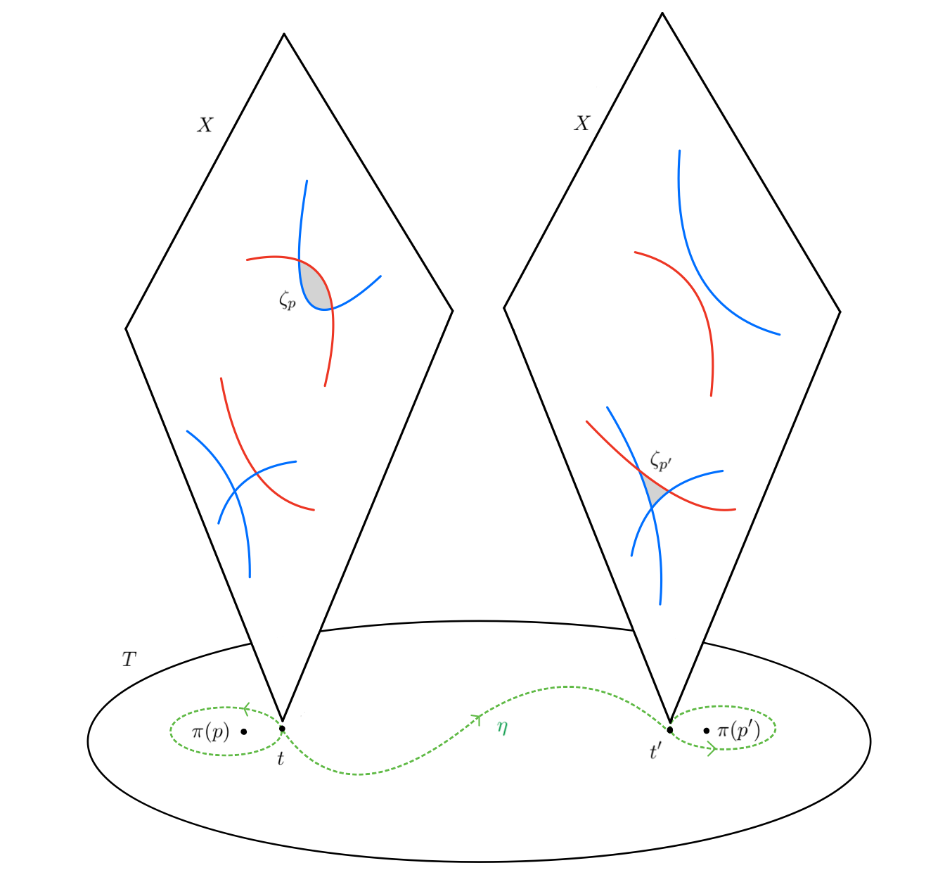
Figure 13. Iterated variation around two critical values.

By the Picard-Lefschetz theorem, $\operatorname{Var}_{p}$ maps any class in $H_{n}(X\setminus A,B)_{t}$ to a multiple of the vanishing cycle $\nu_{p}$. So if $\operatorname{Var}_{p^{\prime}}(\eta_{*}\nu_{p})=0$, it follows that the iterated variation $\operatorname{Var}_{p^{\prime}}\circ\operatorname{Var}_{p}$ is zero. Rewriting the intersection number

$$\langle{\widetilde{\nu}_{p^{\prime}}}\,|\,{\nu_{p}}\rangle=\pm\langle{\partial_{K^{\prime}}\zeta_{p^{\prime}}}\,|\,{\partial_{K^{\prime}}\nu_{p}}\rangle=\pm\langle{\partial_{J}\widetilde{\nu}_{p^{\prime}}}\,|\,{\partial_{J}\zeta_{p}}\rangle$$

as in 3.24, we see that such vanishing is implied by $\partial_{K^{\prime}}\nu_{p}=0$ or $\partial_{J}\widetilde{\nu}_{p^{\prime}}=0$. This observation leads directly to the hierarchy in (4.3) below. However, intersection theory is not required to explain this phenomenon; what matters more fundamentally is the factorization of $\operatorname{Var}_{p}$—through $\partial_{K}$ in the domain, and through $\delta_{J}$ in the codomain (3.11 and 3.33).

The cycle $\nu_{p}$ is supported in a small ball $W_{p}$ that intersects only those $A_{j}$ and $B_{k}$ where $j\in J$ and $k\in K$ are in the type $(J,K)$ of $p$. For any other boundary component ($k\notin K$), we have $W_{p}\cap B_{k}=\varnothing$ and $\partial_{B_{k}}\nu_{p}=0$. After continuation to $t^{\prime}$, the cycle $\eta_{*}\nu_{p}$ need not be contained in any small ball anymore—but it does stay away from $B_{k}$ and so $\partial_{B_{k}}\eta_{*}\nu_{p}=0$, for $k\notin K$. This follows from the diagram

where $B^{\prime}=\bigcup_{i\neq k}B_{i}$. The diagram commutes (see section B.3), because an isotopy of the stratified set $D$ descends to compatible local trivializations of the fibre bundles $(Y\setminus A,B)$ and $(B_{k}\setminus A,B^{\prime})$ over $T\setminus L$, and furthermore the isotopy can be chosen to be smooth.

As pointed out in 3.24 and 3.33, the variation $\operatorname{Var}_{p^{\prime}}$ factors through the iterated boundary $\partial_{K^{\prime}}$ of the second simple pinch $p^{\prime}$ with type $(J^{\prime},K^{\prime})$. So if $K^{\prime}\setminus K$ is non-empty, and hence $\partial_{K^{\prime}}\eta_{*}\nu_{p}=0$ as explained above, it follows that $\operatorname{Var}_{p^{\prime}}(\eta_{*}\nu_{p})=0$. We conclude that

(4.1) $$\operatorname{Var}_{p^{\prime}}\circ\operatorname{Var}_{p}=0\quad\text{if $K^{\prime}\nsubseteq K$}.$$

Now consider some $j\in J$ and let $A^{\prime}=\bigcup_{i\neq j}A_{i}$. As a coboundary around $A_{j}$, the vanishing cycle $\nu_{p}$ becomes zero under the inclusion $\kappa\colon Y\setminus A\hookrightarrow Y\setminus A^{\prime}$, because the composition $\kappa_{*}\delta_{j}=0$ vanishes as part of the residue sequence

$$H_{n-1}(A_{j}\setminus A^{\prime},B)_{t}\xrightarrow{\delta_{j}}H_{n}(Y\setminus A,B)_{t}\xrightarrow{\kappa_{*}}H_{n}(Y\setminus A^{\prime},B)_{t}.$$

As discussed above, such vanishing $\kappa_{*}\nu_{p}=0$ persists by parallel transport also at $t^{\prime}$, whence $\kappa_{*}(\eta_{*}\nu_{p})=0$. If $A_{j}$ does not contain $p^{\prime}$, then $A_{j}$ does not intersect the ball $W_{p^{\prime}}$ and so $W_{p^{\prime}}\setminus A=W_{p^{\prime}}\setminus A^{\prime}$. Then the trace map $W_{p^{\prime}*}$ factors through $\kappa_{*}$, and thus annihilates the vanishing cycle. It follows that

(4.2) $$\operatorname{Var}_{p^{\prime}}\circ\operatorname{Var}_{p}=0\quad\text{if $J^{\prime}\nsupseteq J$}.$$

Definition 4.2.

We define a relation on the set of simple pinches as follows: For simple pinches $p$ and $p^{\prime}$ with type $(J,K)$ and $(J^{\prime},K^{\prime})$, we set

$$p^{\prime}\leqslant p\quad\text{if}\quad\text{$J^{\prime}\supseteq J$ and $K^{\prime}\subseteq K$}.$$

This relation is transitive and reflexive (a preorder). We can then summarize the observations made above as

(4.3) $$\operatorname{Var}_{p^{\prime}}\circ\operatorname{Var}_{p}=0\quad\text{whenever}\quad p^{\prime}\nleqslant p.$$

Remark 4.3.

These conclusions about variations at simple pinches hold also in the presence of further, non-simple critical points.

4.2. Linear and quadratic refinements

For a linear pinch $p$, the boundary $\partial_{K}\nu_{p}=\pm\iota_{p*}\delta_{J}\partial_{1,\ldots,n+1}\zeta=0$ of the vanishing cell (simplex) is empty. In addition to the vanishing (4.1) for $K^{\prime}\setminus K\neq\varnothing$, we therefore also have

(4.4) $$\operatorname{Var}_{p^{\prime}}\circ\operatorname{Var}_{p}=0\quad\text{if}\quad\big{(}\text{$K^{\prime}=K$ and $p$ linear}\big{)}.$$

Similarly, if $p^{\prime}$ is a linear pinch, then $\partial_{J^{\prime}}\widetilde{\nu}_{p^{\prime}}=0$ extends the vanishing (4.2) by the additional constraint

(4.5) $$\operatorname{Var}_{p^{\prime}}\circ\operatorname{Var}_{p}=0\quad\text{if}\quad\big{(}\text{$J^{\prime}=J$ and $p^{\prime}$ linear}\big{)}.$$

Corollary 4.4.

If all critical points are linear pinches, then $\operatorname{Var}_{p^{\prime}}\circ\operatorname{Var}_{p}$ can only be non-zero if $J^{\prime}\supset J$ and $K^{\prime}\subset K$ are strict inclusions. Hence in this situation, the monodromy representation is unipotent: every sequence of $n$ or more variations is zero. We discuss this further in section 5.1.

From (3.12), we also know that for a linear or quadratic simple pinch $p$ on a stratum with codimension $m=\lvert J\rvert+\lvert K\rvert$, the repeated variation vanishes,

(4.6) $$\operatorname{Var}_{p}\circ\operatorname{Var}_{p}=0\quad\text{if}\quad\text{$n-m$ is odd.}$$

This applies in particular to linear pinches ($m=n+1$).

Remark 4.5.

We can incorporate the additional constraints (4.4)–(4.6) into (4.3) by removing the relations $p^{\prime}\leqslant p$ among those particular pairs of pinches. The resulting relation is still transitive, but not necessarily reflexive anymore.

4.3. A hierarchy on simple pinch components

Over every irreducible component $\ell\subseteq L$ of the Landau variety, we may have several critical strata. Suppose that $\ell$ is a simple pinch component (3.14), that is, all critical points over a generic point $t_{c}\in\ell$ are simple pinches. Let $P_{\ell}\subset\pi^{-1}(t_{c})$ denote these pinches. Recall from 3.15 that

$$\operatorname{Var}_{\ell}=\sum_{p\in P_{\ell}}\operatorname{Var}_{p},$$

where we write $\operatorname{Var}_{\ell}$ for the variation $\operatorname{Var}_{\gamma}$ along a simple loop around $t_{c}\in\ell$. The operator $\operatorname{Var}_{\ell}$ does depend on the choice of $\gamma$, but this choice is irrelevant for the following vanishing results. Furthermore, we write $\operatorname{Var}_{\ell^{\prime}}\circ\operatorname{Var}_{\ell}$ to abbreviate $\eta_{*}^{-1}\operatorname{Var}_{\ell^{\prime}}\eta_{*}\operatorname{Var}_{\ell}$, as above.

Definition 4.6.

Define a binary relation $\leqslant$ on the set of simple pinch components of the Landau variety as follows:

$$\ell^{\prime}\leqslant\ell\quad\text{if there exist $p\in P_{\ell}$ and $p^{\prime}\in P_{\ell^{\prime}}$ such that $p^{\prime}\leqslant p$.}$$

Corollary 4.7.

For any pair $\ell,\ell^{\prime}\subseteq L$ of simple pinch components, we have

$$\operatorname{Var}_{\ell^{\prime}}\circ\operatorname{Var}_{\ell}=0\quad\text{if}\quad\ell^{\prime}\nleqslant\ell.$$

Due to the arbitrariness of the intermediate path $\eta$ in section 4.1, we have actually shown that for arbitrary paths $\gamma\in\pi_{1}(T\setminus L,t_{0})$,

$$\operatorname{Var}_{\ell^{\prime}}\circ\operatorname{Var}_{\gamma}\circ\operatorname{Var}_{\ell}=0\quad\text{if}\quad\ell^{\prime}\nleqslant\ell.$$

4.4. Generalization

Above, we derived the hierarchy principle as a consequence of the explicit Picard-Lefschetz formula for (arbitrary) simple pinches, as characterized by the local description (3.22). What is “simple” about these critical points $p\in cS$ is not just that they are (fibrewise) isolated, but furthermore that the exclusion of any of the supporting hypersurfaces from the arrangement removes the critical point. We will demonstrate below that the latter property is sufficient to explain the hierarchy principle—without any recourse to the Picard-Lefschetz formula. This discussion will lead to a generalization of the hierarchy principle to “non-simple” critical points.

Consider some generic critical value $t_{c}\in\ell\subseteq L$. The corresponding critical points $P=\bigcup_{S\in\mathfrak{S}}cS\cap\pi^{-1}(t_{c})$ need not be isolated; they form some closed subvariety $P\subset X$. In any case, we expect some form of the localization from section 3.2: For every connected component $p\in\pi_{0}(P)$, suppose we can find a smooth manifold $W_{p}\subset X$ containing $p\subset W_{p}$, not intersecting any other components of $P$, and such that its boundary $\partial W_{p}$ is smooth and transverse to $D$. Then the proof of 3.15 still applies, so that

$$\operatorname{Var}_{\ell}=\sum_{p\in\pi_{0}(P)}\operatorname{Var}_{p}\quad\text{with}\quad\operatorname{Var}_{p}=\iota_{p*}\operatorname{var}_{p}W_{p*}$$

where $\operatorname{var}_{p}$ is defined just as in 3.11. For example, if $p\in\pi_{0}(P)$ is a smooth component, we can construct $W_{p}$ as a tubular neighbourhood of $p$. For an isolated point $p$, this reproduces the balls used in section 3.3.

Definition 4.8.

The type $(J,K)$ of a critical component $p\in\pi_{0}(P)$ is the set of those hypersurfaces $A_{j}$ ($j\in J$) and $B_{k}$ ($k\in K$) which intersect $p$.

Note that if we choose $W_{p}$ small enough, then it will intersect only the hypersurfaces in the type of $p$: $W_{p}\cap A=W_{p}\cap A_{J}$ and $W_{p}\cap B=W_{p}\cap B_{K}$. Then the trace $W_{p*}$ factors through the inclusion $X\setminus A\hookrightarrow X\setminus A_{J}$, and $\iota_{p*}$ factors through the map of pairs $(X\setminus A,B_{K})\rightarrow(X\setminus A,B)$:

(4.7) $$\begin{gathered}\lx@xy@svg{\hbox{\raise 0.0pt\hbox{\kern 77.59584pt\hbox{\ignorespaces\ignorespaces\ignorespaces\hbox{\vtop{\kern 0.0pt\offinterlineskip\halign{\entry@#!@&&\entry@@#!@\cr&\\&\\&\\}}}\ignorespaces{\hbox{\kern-34.80455pt\raise 0.0pt\hbox{\hbox{\kern 0.0pt\raise 0.0pt\hbox{\hbox{\kern 3.0pt\raise 0.0pt\hbox{$\textstyle{H_{n}(X\setminus A,B)_{t}\ignorespaces\ignorespaces\ignorespaces\ignorespaces\ignorespaces\ignorespaces\ignorespaces\ignorespaces\ignorespaces\ignorespaces\ignorespaces\ignorespaces\ignorespaces}$}}}}}}}\ignorespaces\ignorespaces\ignorespaces\ignorespaces\ignorespaces{}{}{}{{}{}{}{}{}{}{}{}{}{}{}{}{}{}{}}{}\ignorespaces\hbox{\hbox{\kern 0.0pt\raise 0.0pt\hbox{{}{}{{}}{{}{}{}}{}}}}\ignorespaces{}\ignorespaces{}{}{}{{}{}}\ignorespaces\ignorespaces{\hbox{\kern-77.59584pt\raise-40.0pt\hbox{{}\hbox{\kern 0.0pt\raise 0.0pt\hbox{\hbox{\kern 3.0pt\hbox{\hbox{\kern 0.0pt\raise-1.5375pt\hbox{$\scriptstyle{W_{p*}}$}}}\kern 3.0pt}}}}}}\ignorespaces{}{}{}{{}{}{}{}{}{}{}{}{}{}{}{}{}{}{}{}{}{}{}{}{}{}}{\hbox{\kern-27.36131pt\raise-69.50195pt\hbox{\hbox{\kern 0.0pt\raise 0.0pt\hbox{\lx@xy@tip{1}\lx@xy@tip{-1}}}}}}\ignorespaces\hbox{\hbox{\kern 0.0pt\raise 0.0pt\hbox{{}{}{}{{}}{{}{}{}\lx@xy@spline@}{}}}}\ignorespaces{}\ignorespaces\hbox{\hbox{\kern 0.0pt\raise 0.0pt\hbox{{}{}{{}}{{}{}{}}{}}}}\ignorespaces{}\ignorespaces\ignorespaces\ignorespaces\ignorespaces{}{\hbox{\lx@xy@droprule}}\ignorespaces{\hbox{\kern 0.0pt\raise-29.5pt\hbox{\hbox{\kern 0.0pt\raise 0.0pt\hbox{\lx@xy@tip{1}\lx@xy@tip{-1}}}}}}{\hbox{\lx@xy@droprule}}{\hbox{\lx@xy@droprule}}\ignorespaces\ignorespaces\ignorespaces\ignorespaces{}{\hbox{\lx@xy@droprule}}\ignorespaces\ignorespaces\ignorespaces{\hbox{\kern 40.24783pt\raise 6.2111pt\hbox{{}\hbox{\kern 0.0pt\raise 0.0pt\hbox{\hbox{\kern 3.0pt\hbox{\hbox{\kern 0.0pt\raise-1.57222pt\hbox{$\scriptstyle{\operatorname{Var}_{p}}$}}}\kern 3.0pt}}}}}}\ignorespaces{\hbox{\kern 65.19528pt\raise 0.0pt\hbox{\hbox{\kern 0.0pt\raise 0.0pt\hbox{\lx@xy@tip{1}\lx@xy@tip{-1}}}}}}{\hbox{\lx@xy@droprule}}{\hbox{\lx@xy@droprule}}{\hbox{\kern 65.19528pt\raise 0.0pt\hbox{\hbox{\kern 0.0pt\raise 0.0pt\hbox{\hbox{\kern 3.0pt\raise 0.0pt\hbox{$\textstyle{H_{n}(X\setminus A,B)_{t}}$}}}}}}}{\hbox{\kern-36.6265pt\raise-40.0pt\hbox{\hbox{\kern 0.0pt\raise 0.0pt\hbox{\hbox{\kern 3.0pt\raise 0.0pt\hbox{$\textstyle{H_{n}(X\setminus A_{J},B)_{t}\ignorespaces\ignorespaces\ignorespaces\ignorespaces}$}}}}}}}\ignorespaces\ignorespaces\ignorespaces\ignorespaces{}{\hbox{\lx@xy@droprule}}\ignorespaces{\hbox{\kern 0.0pt\raise-69.5pt\hbox{\hbox{\kern 0.0pt\raise 0.0pt\hbox{\lx@xy@tip{1}\lx@xy@tip{-1}}}}}}{\hbox{\lx@xy@droprule}}{\hbox{\lx@xy@droprule}}{\hbox{\kern 62.61694pt\raise-40.0pt\hbox{\hbox{\kern 0.0pt\raise 0.0pt\hbox{\hbox{\kern 3.0pt\raise 0.0pt\hbox{$\textstyle{H_{n}(X\setminus A,B_{K})_{t}\ignorespaces\ignorespaces\ignorespaces\ignorespaces}$}}}}}}}\ignorespaces\ignorespaces\ignorespaces\ignorespaces{}{\hbox{\lx@xy@droprule}}\ignorespaces{\hbox{\kern 99.99983pt\raise-5.5pt\hbox{\hbox{\kern 0.0pt\raise 0.0pt\hbox{\lx@xy@tip{1}\lx@xy@tip{-1}}}}}}{\hbox{\lx@xy@droprule}}{\hbox{\lx@xy@droprule}}{\hbox{\kern-35.04793pt\raise-80.0pt\hbox{\hbox{\kern 0.0pt\raise 0.0pt\hbox{\hbox{\kern 3.0pt\raise 0.0pt\hbox{$\textstyle{H_{n}(\overline{W_{p}}\setminus A_{J},B_{K})\ignorespaces\ignorespaces\ignorespaces\ignorespaces}$}}}}}}}\ignorespaces\ignorespaces\ignorespaces\ignorespaces{}{\hbox{\lx@xy@droprule}}\ignorespaces\ignorespaces\ignorespaces{\hbox{\kern 41.22005pt\raise-74.67361pt\hbox{{}\hbox{\kern 0.0pt\raise 0.0pt\hbox{\hbox{\kern 3.0pt\hbox{\hbox{\kern 0.0pt\raise-0.6875pt\hbox{$\scriptstyle{\operatorname{var}_{p}}$}}}\kern 3.0pt}}}}}}\ignorespaces{\hbox{\kern 60.6265pt\raise-80.0pt\hbox{\hbox{\kern 0.0pt\raise 0.0pt\hbox{\lx@xy@tip{1}\lx@xy@tip{-1}}}}}}{\hbox{\lx@xy@droprule}}{\hbox{\lx@xy@droprule}}{\hbox{\kern 60.6265pt\raise-80.0pt\hbox{\hbox{\kern 0.0pt\raise 0.0pt\hbox{\hbox{\kern 3.0pt\raise 0.0pt\hbox{$\textstyle{H_{n}(W_{p}\setminus A_{J},B_{K})\ignorespaces\ignorespaces\ignorespaces\ignorespaces\ignorespaces\ignorespaces\ignorespaces\ignorespaces\ignorespaces}$}}}}}}}\ignorespaces\ignorespaces\ignorespaces\ignorespaces{}{\hbox{\lx@xy@droprule}}\ignorespaces{\hbox{\kern 99.99983pt\raise-45.5pt\hbox{\hbox{\kern 0.0pt\raise 0.0pt\hbox{\lx@xy@tip{1}\lx@xy@tip{-1}}}}}}{\hbox{\lx@xy@droprule}}{\hbox{\lx@xy@droprule}}\ignorespaces\ignorespaces\ignorespaces\ignorespaces\ignorespaces{}{}{}{{}{}{}{}{}{}{}{}{}{}{}{}{}{}{}}{}\ignorespaces\hbox{\hbox{\kern 0.0pt\raise 0.0pt\hbox{{}{}{{}}{{}{}{}}{}}}}\ignorespaces{}\ignorespaces{}{}{}{{}{}}\ignorespaces\ignorespaces{\hbox{\kern 159.99983pt\raise-40.0pt\hbox{{}\hbox{\kern 0.0pt\raise 0.0pt\hbox{\hbox{\kern 3.0pt\hbox{\hbox{\kern 0.0pt\raise-0.65279pt\hbox{$\scriptstyle{\iota_{p*}}$}}}\kern 3.0pt}}}}}}\ignorespaces{}{}{}{{}{}{}{}{}{}{}{}{}{}{}{}{}{}{}{}{}{}{}{}{}{}}{\hbox{\kern 115.36041pt\raise-5.49805pt\hbox{\hbox{\kern 0.0pt\raise 0.0pt\hbox{\lx@xy@tip{1}\lx@xy@tip{-1}}}}}}\ignorespaces\hbox{\hbox{\kern 0.0pt\raise 0.0pt\hbox{{}{}{}{{}}{{}{}{}\lx@xy@spline@}{}}}}\ignorespaces{}\ignorespaces\hbox{\hbox{\kern 0.0pt\raise 0.0pt\hbox{{}{}{{}}{{}{}{}}{}}}}\ignorespaces{}\ignorespaces}}}}\ignorespaces\end{gathered} \textstyle{H_{n}(X\setminus A,B)_{t}\ignorespaces\ignorespaces\ignorespaces\ignorespaces\ignorespaces\ignorespaces\ignorespaces\ignorespaces\ignorespaces\ignorespaces\ignorespaces\ignorespaces\ignorespaces} \scriptstyle{W_{p*}} \scriptstyle{\operatorname{Var}_{p}} \textstyle{H_{n}(X\setminus A,B)_{t}} \textstyle{H_{n}(X\setminus A_{J},B)_{t}\ignorespaces\ignorespaces\ignorespaces\ignorespaces} \textstyle{H_{n}(X\setminus A,B_{K})_{t}\ignorespaces\ignorespaces\ignorespaces\ignorespaces} \textstyle{H_{n}(\overline{W_{p}}\setminus A_{J},B_{K})\ignorespaces\ignorespaces\ignorespaces\ignorespaces} \scriptstyle{\operatorname{var}_{p}} \textstyle{H_{n}(W_{p}\setminus A_{J},B_{K})\ignorespaces\ignorespaces\ignorespaces\ignorespaces\ignorespaces\ignorespaces\ignorespaces\ignorespaces\ignorespaces} \scriptstyle{\iota_{p*}} \textstyle{H_{n}(X\setminus A,B)_{t}\ignorespaces\ignorespaces\ignorespaces\ignorespaces\ignorespaces\ignorespaces\ignorespaces\ignorespaces\ignorespaces\ignorespaces\ignorespaces\ignorespaces\ignorespaces} \scriptstyle{W_{p*}} \scriptstyle{\operatorname{Var}_{p}} \textstyle{H_{n}(X\setminus A,B)_{t}} \textstyle{H_{n}(X\setminus A_{J},B)_{t}\ignorespaces\ignorespaces\ignorespaces\ignorespaces} \textstyle{H_{n}(X\setminus A,B_{K})_{t}\ignorespaces\ignorespaces\ignorespaces\ignorespaces} \textstyle{H_{n}(\overline{W_{p}}\setminus A_{J},B_{K})\ignorespaces\ignorespaces\ignorespaces\ignorespaces} \scriptstyle{\operatorname{var}_{p}} \textstyle{H_{n}(W_{p}\setminus A_{J},B_{K})\ignorespaces\ignorespaces\ignorespaces\ignorespaces\ignorespaces\ignorespaces\ignorespaces\ignorespaces\ignorespaces} \scriptstyle{\iota_{p*}}$$

The hierarchy constraints arise from hypersurfaces in the type that are indispensable to make $p$ critical. We call those hypersurfaces simple.

Definition 4.9.

Given a critical component $p\in\pi_{0}(P)$ of type $(J,K)$, we call an element $i\in J\sqcup K$ and the corresponding hypersurface $D_{i}$ simple if the union $\bigcup_{k\neq i}D_{k}$ of all other components of $D$ has no critical points in $p$. We denote the simple elements of the type as $J_{\mathsf{s}}\subseteq J$ and $K_{\mathsf{s}}\subseteq K$.

Remark 4.10.

For a simple pinch, omitting any hypersurface $D_{1},\ldots,D_{m}$ in (3.22) results in a non-critical arrangement. Therefore, the entire type is simple: $(J_{\mathsf{s}},K_{\mathsf{s}})=(J,K)$. In fact, this property characterizes simple pinches topologically: Every isolated critical point with $(J_{\mathsf{s}},K_{\mathsf{s}})=(J,K)$ admits local coordinates of the form (3.22).

Non-simple situations can arise even for isolated critical points, for example if one starts with a simple pinch $p$ and then enlarges the arrangement by an additional hyperplane that contains $p$.

Example 4.11.

Consider $Y=X\times T=\mathbb{P}^{1}\times\mathbb{C}$ with the transverse arrangement $D=D_{1}\cup D_{2}$ formed by the smooth hypersurfaces $D_{1}=\{x^{2}=t\}$ and $D_{2}=\{x=0\}$ in coordinates $[x:1]\in\mathbb{P}^{1}$. The pair $(Y,D)$ has a single critical point, $c(D_{1}\cap D_{2})=\{(p,t_{c})\}$ over $t_{c}=0$, namely $p=[0:1]$.

• $D_{1}$ is simple: The remaining pair $(Y,D_{2})\cong(\mathbb{P}^{1},\{p\})\times\mathbb{C}$ is a (trivial) fibre bundle, without any critical points.

• $D_{2}$ is not simple: Even after removing $D_{2}$, the remaining pair $(Y,D_{1})$ still has $c(D_{1})=\{(p,t_{c})\}$ as a critical point.

For simple pinches, the hierarchy follows from the factorization (3.24) of $\operatorname{var}_{p}$ through each $\partial_{k}$ in the domain, and each $\delta_{j}$ in the codomain. For general critical sets, such a factorization applies only to the simple indices. Given an index $k\in K$ or $j\in J$, consider the natural map of pairs

$$\rho_{k}\colon \textstyle(X\setminus A,\bigcup_{i\neq k}B_{i}) \rightarrow(X\setminus A,B),$$

$$\kappa_{j}\colon (X\setminus A,B) \textstyle\rightarrow(X\setminus\bigcup_{i\neq j}A_{i},B).$$

Lemma 4.12.

Let $p\in\pi_{0}(P)$ with type $(J,K)$ and simple part $(J_{\mathsf{s}},K_{\mathsf{s}})$. Then for every $k\in K_{\mathsf{s}}$, and for every $j\in J_{\mathsf{s}}$, we have

(4.8) $$\kappa_{j*}\operatorname{Var}_{p}=0\qquad\text{and}\qquad\operatorname{Var}_{p}\rho_{k*}=0.$$

Equivalently, the local variation at $p$ factors through the boundary map $\partial_{k}$ in the domain, and through the Leray coboundary $\delta_{j}$ in the codomain.

Proof.

Let $A^{\prime}=\bigcup_{i\neq j}A_{i}$ and $B^{\prime}=\bigcup_{i\neq k}B_{i}$ denote the arrangements $A$ and $B$, with one of the simple indices omitted. By 4.9, the corresponding pairs $(W_{p}\setminus A^{\prime},B)$ and $(W_{p}\setminus A,B^{\prime})$ are locally trivial even over the critical value $\{t_{c}\}=\pi(P)$. Hence they have trivial monodromy and zero variation.

In the domain, this implies that the local variation $\operatorname{Var}_{p}$ vanishes on the image of the push-forward of the map $\rho\colon(X\setminus A,B^{\prime})\rightarrow(X\setminus A,B)$. By the long exact boundary sequence (3.9), this image equals the kernel of $\partial_{k}$, thus $\operatorname{Var}_{p}$ factors through $\partial_{k}$:

In the codomain, the zero variation of $(W_{p}\setminus A^{\prime},B)$ implies that $\operatorname{Var}_{p}$ takes values in the kernel of $\kappa_{*}$, where $\kappa\colon(X\setminus A,B)\rightarrow(X\setminus A^{\prime},B)$:

By the long exact residue sequence, the kernel of $\kappa_{*}$ is the image of $\delta_{j}$. ∎

$\overset{g_{*}}{\longmapsto}\$

$\Rightarrow\operatorname{Var}_{p}h=$

$\overset{g_{*}}{\longmapsto}\$ $\Rightarrow\operatorname{Var}_{p}h=$

Figure 14. Non-vanishing variations at a non-simple isolated singularity (4.13).

Example 4.13.

Consider 4.11 with the partition $(A,B)=(D_{1},D_{2})$. As illustrated in fig. 14, the variation $\operatorname{Var}_{p}h$ is a coboundary around $D_{1}$ as expected ($1\in J_{\mathsf{s}}$). But it is non-zero, despite $\partial_{2}h=0$, so $\operatorname{Var}_{p}$ does not factor through $\partial_{2}$ in the domain. The case $(A,B)=(D_{2},D_{1})$ demonstrates that the variation $\operatorname{Var}_{p}h$ need not be a coboundary around the non-simple hypersurface $D_{2}$.

Remark 4.14.

If there are two simple types $j,j^{\prime}\in J_{\mathsf{s}}$, then 4.12 states that $\nu=\operatorname{Var}_{p}h$ can be written as a coboundary $\nu=\delta_{j}\alpha$ around $A_{j}$, and also as a coboundary $\nu=\delta_{j^{\prime}}\alpha^{\prime}$ around $A_{j^{\prime}}$. This does not necessarily imply that $\nu=\delta_{j}\delta_{j^{\prime}}\alpha^{\prime\prime}$ is an iterated coboundary [65]. Similarly, for two simple types $k,k^{\prime}\in K_{\mathsf{s}}$, it is not necessarily the case that $\operatorname{Var}_{p}h$ depends only on the iterated boundary $\partial_{k}\partial_{k^{\prime}}h$.

Definition 4.15.

Suppose that $p\subset\pi^{-1}(t_{c})$ and $p^{\prime}\subset\pi^{-1}(t_{c}^{\prime})$ are connected components of the critical sets in two fibres. Let $(J,K),(J^{\prime},K^{\prime})$ denote the types of $p,p^{\prime}$ and $(J_{\mathsf{s}},K_{\mathsf{s}}),(J^{\prime}_{\mathsf{s}},K_{\mathsf{s}}^{\prime})$ their simple parts. We then declare $p^{\prime}$ and $p$ to be compatible,

$$p^{\prime}\leqslant p,\qquad\text{if}\qquad K^{\prime}_{\mathsf{s}}\subseteq K\quad\text{and}\quad J_{\mathsf{s}}\subseteq J^{\prime}.$$

For simple pinches, this relation is just 4.2, due to 4.10.

Corollary 4.16.

If $p^{\prime}\nleqslant p$, then $\operatorname{Var}_{p^{\prime}}\circ\operatorname{Var}_{p}=0$.

Proof.

Combine the factorization (4.7) with the vanishing (4.8). For example, if $k\in K_{\mathsf{s}}^{\prime}\setminus K$, then $\iota_{p*}$ factors through $\rho_{k*}$, which is annihilated by $\operatorname{Var}_{p^{\prime}}$. ∎

We can now formulate the general hierarchy principle. It enforces the vanishing of certain iterated variations, and it follows from the previous constraints on $\operatorname{Var}_{p^{\prime}}\circ\operatorname{Var}_{p}=0$, together with the localization $\operatorname{Var}_{\ell}=\sum_{p}\operatorname{Var}_{p}$ discussed at the beginning of section 4.4.

Definition 4.17.

Let $\mathfrak{L}$ denote the set of Landau singularities, that is, the set of irreducible components of the Landau variety that have complex codimension one. Define a binary relation $\leqslant$ on $\mathfrak{L}$ as follows: For $\ell\in\mathfrak{L}$, let $P_{\ell}\subset\pi^{-1}(t_{c})$ denote the critical set in a fibre over a generic point $t_{c}\in\ell$. Then set $\ell^{\prime}\leqslant\ell$ if and only if there exist $p\in P_{\ell}$ and $p^{\prime}\in P_{\ell^{\prime}}$ such that $p^{\prime}\leqslant p$.

Corollary 4.18.

For any pair $\ell,\ell^{\prime}\in\mathfrak{L}$ of Landau singularities, we have

$$\operatorname{Var}_{\ell^{\prime}}\circ\operatorname{Var}_{\ell}=0\quad\text{if}\quad\ell^{\prime}\nleqslant\ell.$$

5. Polylogarithms

In this section, we illustrate the hierarchy principle with polylogarithms. The most generic situation, Aomoto polylogarithms, is the simplest—all critical points are linear simple pinches. In section 5.2, we also discuss the hierarchy for the dilogarithm, which involves non-isolated critical sets.

5.1. Aomoto polylogarithms

A collection $Q=Q_{0}\cup\ldots\cup Q_{n}$ of $n+1$ hyperplanes in complex projective space $\mathbb{P}^{n}$ is called a simplex. We say that it is non-degenerate if the intersection $Q_{0}\cap\ldots\cap Q_{n}$ is empty.

To a pair of non-degenerate simplices $Q$ and $R$, we associate:

• a differential form $\omega_{Q}$ with simple poles on each $Q_{i}$ that generates $H_{\mathsf{dR}}^{n}(\mathbb{P}^{n}\setminus Q)\cong\mathbb{C}$. In terms of linear equations $f_{i}=0$ for $Q_{i}$,

  (5.1) $$\omega_{Q}=\mathrm{d}\log\left(\frac{f_{1}}{f_{0}}\right)\wedge\ldots\wedge\mathrm{d}\log\left(\frac{f_{n}}{f_{0}}\right).$$

• a generator $\sigma_{R}\in H_{n}(\mathbb{P}^{n},R)\cong\mathbb{Z}$ corresponding to the real standard simplex $\{\sum_{i}u_{i}=1\}\subset\mathbb{R}_{\geq 0}^{n+1}$, embedded as $\{[u_{0}:\cdots:u_{n}]\colon u_{i}\geq 0\}\subset\mathbb{P}^{n}$ with boundary in $R$, in coordinates $u$ where $R_{i}=\{u_{i}=0\}$.

Suppose that $\sigma_{R}$ can be deformed to avoid $Q$, so that $\sigma_{R}$ has a preimage $\sigma_{R}^{\prime}\in H_{n}(\mathbb{P}^{n}\setminus Q,R)$ under the inclusion of pairs $(\mathbb{P}^{n}\setminus Q,R\setminus Q)\rightarrow(\mathbb{P}^{n},R)$.

The Aomoto polylogarithm [2, §2] of weight $n$ is the integral

$$\Lambda_{n}(Q,R)=\int_{\sigma_{R}^{\prime}}\omega_{Q}.$$

It depends on the choice of $\sigma_{R}^{\prime}$, hence $\Lambda_{n}$ is a multivalued function on the space $T=(\mathbb{P}^{n})^{2n+2}$ of pairs $t=(Q_{0},\ldots,Q_{n},R_{0},\ldots,R_{n})$ of simplices. We identify hyperplanes $Q_{i}\subset X=\mathbb{P}^{n}$ with points $[Q_{0i}:\cdots:Q_{ni}]$ in the dual $\mathbb{P}^{n}$, and we can represent points $t\in T$ as $(n+1)\times(2n+2)$ matrices with column vectors $Q_{i}=(Q_{0i},\ldots,Q_{ni})^{\intercal},R_{j}=(R_{0j},\ldots,R_{nj})^{\intercal}$. We obtain an arrangement $A\cup B$ in the total space $Y=X\times T$, with the components

$$\mathfrak{A} =\{A_{0},\ldots,A_{n}\},\quad A_{i}=\big{\{}x_{0}Q_{0i}+\ldots+x_{n}Q_{ni}=0\big{\}}\subset Y,$$

$$\mathfrak{B} =\{B_{0},\ldots,B_{n}\},\quad B_{j}=\big{\{}x_{0}R_{0j}+\ldots+x_{n}R_{nj}=0\big{\}}\subset Y.$$

Lemma 5.1.

The divisor $A\cup B$ has simple normal crossings.

Proof.

At every point $[p_{0}:\cdots:p_{n}]\in X$ we can find $k$ such that $p_{k}\neq 0$. If $(p,t)\in A_{i}$, there must be an index $r\neq k$ such that $Q_{ri}\neq 0$, for otherwise, the equation of $A_{i}$ would collapse at $p$ to $p_{k}Q_{ki}=0$ and imply $Q_{i}=0\notin\mathbb{P}^{n}$. So after relabelling, we may assume that $p_{0}=Q_{1i}=1$. It follows that at $p$, and hence in a small neighbourhood, the functions

$$z^{(i)}=(z_{1}^{(i)},\ldots,z_{n}^{(i)})=(Q_{0i}+p_{1}+p_{2}Q_{2i}+\ldots+p_{n}Q_{ni},Q_{2i},\ldots,Q_{ni})$$

form a coordinate chart of the $\mathbb{P}^{n}$ that parametrizes the hyperplane $Q_{i}$. This way, we can locally choose coordinates $(z^{(0)},\ldots,z^{(2n+1)})$ on the product $T=(\mathbb{P}^{n})^{2n+2}$ such that $A_{i}=\{z_{1}^{(i)}=0\}$ and $B_{j}=\{z_{1}^{(n+1+j)}=0\}$. ∎

The strata $S$ of the canonical stratification of $A\cup B$ are indexed by pairs $I,J\subseteq\{0,\ldots,n\}$ so that $\overline{S}=A^{I}\cap B^{J}=\bigcap_{i\in I}A_{i}\cap\bigcap_{j\in J}B_{j}$. It follows from considerations similar to [51, §IV.4.4] that the Landau variety can be computed from the closures of the strata:

$$L=\bigcup_{S\in\mathfrak{S}}\pi(cS)=\bigcup_{S\in\mathfrak{S}}\pi(c\overline{S})=\bigcup_{I,J}\pi(c(A^{I}\cap B^{J})).$$

Let $t_{IJ}=(Q_{i\in I},R_{j\in J})$ denote the submatrix of $t$, consisting of the columns in $I$ and $J$. Write $V_{IJ}\subset\mathbb{C}^{n+1}$ for the vector space spanned by these columns.

Lemma 5.2.

A point $(x,t)$ of the submanifold $A^{I}\cap B^{J}\subset Y$ is critical precisely when the columns $t_{IJ}=(Q_{i\in I},R_{j\in J})$ of $t$ are linearly independent.

Proof.

The submanifold $S=A^{I}\cap B^{J}$ has complex dimension $\dim T+n-k$ with $k=\lvert I\rvert+\lvert J\rvert$. The fibre at $t$ is the projectivization $S_{t}=\mathbb{P}(V_{IJ}^{\perp})\subset\mathbb{P}^{n}$ of

$$V_{IJ}^{\perp}=\bigcap_{v\in V_{IJ}}\{y\in\mathbb{C}^{n+1}\colon x_{0}v_{0}+\ldots+x_{n}v_{n}=0\}\subset\mathbb{C}^{n+1},$$

the annihilator of $V_{IJ}$. Therefore, at any $t\in T$, the fibre $S_{t}=A^{I}\cap B^{J}\cap\pi^{-1}(t)$ is a complex manifold with complex dimension

(5.2) $$\dim S_{t}=\dim V_{IJ}^{\perp}-1=n-\dim V_{IJ}.$$

The kernel of the differential $\mathrm{d}(\pi|_{S})$ is the intersection (in $TY=TX\oplus TT$) of the vectors that are tangent to $S$ ($TS$) and vertical ($TX$). In other words, $\ker\mathrm{d}(\pi|_{S})=T(S_{t})$ is the tangent bundle of the fibre. Hence the image of $\mathrm{d}(\pi|_{S})$ has dimension $\dim S-(n-\dim V_{IJ})=\dim T-(k-\dim V_{IJ})$ and we have a submersion precisely when $\dim V_{IJ}=k$. ∎

The fibre of $A^{I}\cap B^{J}$ over $t$ has dimension $n-\dim V_{IJ}$, see (5.2). In particular, the fibre is empty, unless $\dim V_{IJ}\leq n$.

Corollary 5.3.

The Landau variety of $\pi\colon(Y,A\cup B)\rightarrow T$ is

$$L=\bigcup_{I,J}\big{\{}\mathrm{rank}({t_{IJ}})<\min\{\lvert I\rvert+\lvert J\rvert,n+1\}\big{\}}.$$

For $k=\lvert I\rvert+\lvert J\rvert\leq n+1$, the subvariety $\{\mathrm{rank}({t_{IJ}})<k\}\subset T$ has codimension $n+1-(k-1)$: instead of $n+1$ arbitrary entries, some column is a linear combination of the other $k-1$ columns. Similarly, for $k\geq n+1$ the codimension of the subvariety $\{\mathrm{rank}({t_{IJ}})<n+1\}\subset T$ is $k-n$.

Corollary 5.4.

The components of $L$ with codimension one in $T$ are in bijection with pairs $I,J\subseteq\{0,\ldots,n\}$ so that $\lvert I\rvert+\lvert J\rvert=n+1$. Their form is

$$\ell_{IJ}=\big{\{}\det(t_{IJ})=0\big{\}}\subset T.$$

In fact, $L$ has no irreducible components of higher codimension. For if $k=\lvert I\rvert+\lvert J\rvert\leq n$, then $\{\mathrm{rank}({t_{IJ}})<k\}\subset\ell_{I^{\prime}J^{\prime}}$ for any $I^{\prime}\supseteq I$, $J^{\prime}\supseteq J$ such that $\lvert I^{\prime}\rvert+\lvert J^{\prime}\rvert=n+1$. Similarly, if $k>n+1$, then any $I^{\prime}\subseteq I$, $J^{\prime}\subseteq J$ with $\lvert I^{\prime}\rvert+\lvert J^{\prime}\rvert=n+1$ provide $\{\mathrm{rank}({t_{IJ}})<n+1\}\subset\ell_{I^{\prime}J^{\prime}}$. It follows that

(5.3) $$L=\bigcup_{I,J\colon\lvert I\rvert+\lvert J\rvert=n+1}\ell_{IJ}.$$

At a generic point of $\ell_{IJ}$, we have $\mathrm{rank}({t_{IJ}})=n$ and the one-dimensional kernel of $t_{IJ}$ defines the unique critical point $x$ in the fibre (5.2). It is a linear pinch of type $(I,J)$. The vanishing cell $\zeta_{IJ}$ is a real $n$-simplex bounded by the hyperplanes $Q_{i}$ ($i\in I$) and $R_{j}$ ($j\in J$).

The cases where $I=\varnothing$ or $J=\varnothing$ have zero variation (section 3.7) and the corresponding loci $\ell_{\varnothing,0\ldots n}$ and $\ell_{0\ldots n,\varnothing}$ in $T$ parametrize where $R$, respectively $Q$, become degenerate.

Proposition 5.5.

Let $\varnothing\neq I,J\subseteq\{0,\ldots,n\}$ with $\lvert I\rvert+\lvert J\rvert=n+1$. Then with the intersection number $N=\langle{\partial_{J}\zeta_{IJ}}\,|\,{\partial_{J}\sigma_{R}^{\prime}}\rangle\in\mathbb{Z}$, we have

(5.4) $$\operatorname{Var}_{\ell_{IJ}}\Lambda_{n}(Q,R)=\pm N(2\mathrm{i}\pi)^{|I|}\Lambda_{n-|I|}(\partial_{I}Q,R_{J}\cap Q^{I}).$$

Proof.

The iterated boundary $\partial_{I}\zeta_{IJ}$ is a simplex in $Q^{I}$ bounded by $R_{J}=\bigcup_{j\in J}R_{j}$. By the Picard-Lefschetz and residue formulas eqs. 3.14 and 3.10,

$$\operatorname{Var}_{\ell_{IJ}}\Lambda_{n}(Q,R)=\pm N\int_{\delta_{I}\partial_{I}\zeta_{IJ}}\omega_{Q}=\pm N\cdot(2\mathrm{i}\pi)^{|I|}\int_{\partial_{I}\zeta_{IJ}}\operatorname{Res}_{I}\omega_{Q}$$

is an Aomoto polylogarithm of lower weight. Namely, $\operatorname{Res}_{I}$ denotes the iteration of all residues $\operatorname{Res}_{A_{i}}$ with $i\in I$, and we see from (5.1) that $\operatorname{Res}_{A_{i}}\omega_{Q}=(-1)^{i-1}\omega_{\partial_{i}Q}$. ∎

4.4 states that iterated variations $\operatorname{Var}_{\ell_{I^{\prime}J^{\prime}}}\circ\operatorname{Var}_{\ell_{IJ}}$ are zero, unless $I^{\prime}\supset I$ and $J^{\prime}\subset J$ are strict inclusions. Together with the vanishing of $\operatorname{Var}_{\ell_{IJ}}$ when $I=\varnothing$ or $J=\varnothing$, it follows that any iteration $\operatorname{Var}_{\ell_{I_{k}J_{k}}}\circ\cdots\circ\operatorname{Var}_{\ell_{I_{1}J_{1}}}$ of more than $n$ variations of $\Lambda_{n}$ is zero. This is also clear from (5.4).

Thus, the maximal iterated variations are $n$-fold, and correspond to an increasing sequence $I_{k}=\{\sigma(0),\ldots,\sigma(k-1)\}$ and a decreasing sequence $J_{k}=\{\tau(k),\ldots,\tau(n)\}$. Such sequences encode permutations $\sigma,\tau$ of $\{0,\ldots,n\}$.

Lemma 5.6.

The $n$-fold iterated variations for all permutations $\sigma,\tau$ are

(5.5) $$\operatorname{Var}_{\ell_{\sigma(0)\ldots\sigma(n-1),\tau(n)}}\circ\cdots\circ\operatorname{Var}_{\ell_{\sigma(0),\tau(1)\ldots\tau(n)}}\Lambda_{n}=\pm(2\mathrm{i}\pi)^{n}.$$

Proof.

Iterating 5.5 shows that the iterated variation is an integral multiple of $(2\mathrm{i}\pi)^{n}$. It remains to show that all intersection numbers are $\pm 1$.

For the first intersection, note that the $n$-fold boundaries $\partial_{J_{1}}$ of $\sigma_{R}^{\prime}$ and the first vanishing cell $\zeta_{I_{1}J_{1}}$ are, up to sign, the fundamental class of the (0-dimensional) corner $R^{J_{1}}$ that both simplices share. In particular, in this case where $\lvert J\rvert=n$, the number $N=\pm 1$ in (5.4) only depends on the orientation of $\sigma_{R}$, but not on the choice of lift $\sigma_{R}^{\prime}$.

The subsequent intersections are between the vanishing cycles $\pm\delta_{I_{k}}\partial_{I_{k}}\zeta_{I_{k}J_{k}}$ of the $k$’th variation, and the $(k+1)$’th dual vanishing cycle. Again,

$$\langle{\partial_{J_{k+1}}\zeta_{I_{k+1}J_{k+1}}}\,|\,{\partial_{J_{k+1}}\delta_{I_{k}}\partial_{I_{k}}\zeta_{I_{k}J_{k}}}\rangle=\pm\langle{\partial_{J_{k+1}\sqcup I_{K}}\zeta_{I_{k+1}J_{k+1}}}\,|\,{\partial_{J_{k+1}\sqcup I_{K}}\zeta_{I_{k}J_{k}}}\rangle$$

is the self-intersection of the shared corner $Q^{I_{k}}\cap R^{J_{k+1}}$ of both simplices. ∎

From their differential equations, obtained in [2, §2], it follows that Aomoto polylogarithms are iterated integrals of the differential forms

$$\alpha_{IJ}=\mathrm{d}\log\big{(}\det(t_{IJ})\big{)}.$$

This means that for any base point $t_{0}\in T\setminus L$, there exists a linear combination $W$ of words (tensors) in $\alpha_{IJ}$’s, such that

(5.6) $$\Lambda_{n}(t)=\Lambda_{n}(t_{0})+\int_{t_{0}}^{t}W.$$

Here the integral of a word is defined in terms of a path $\gamma$ from $t_{0}$ to $t$, as

$$\int_{t_{0}}^{t}\alpha_{k}\otimes\cdots\otimes\alpha_{1}=\int_{0}^{1}\gamma^{*}\alpha_{k}(\lambda_{k})\int_{0}^{\lambda_{k}}\gamma^{*}\alpha_{k-1}(\lambda_{k-1})\,\cdots\int_{0}^{\lambda_{2}}\gamma^{*}\alpha_{1}(\lambda_{1}).$$

In the representation (5.6), the variations around $\ell_{IJ}$ can be computed using path concatenation with simple loops. The vanishing of any iteration of more than $n$ variations, dictated by the hierarchy principle as explained above, shows that the words in $W$ must have lengths $k\leq n$.

Corollary 5.7.

The part of $W$ including all words with length $n$ is

(5.7) $$\pm\sum_{\sigma,\tau}(\operatorname{sgn}\sigma)(\operatorname{sgn}\tau)\,\alpha_{\sigma(0)\ldots\sigma(n-1),\tau(n)}\otimes\cdots\otimes\alpha_{\sigma(0),\tau(1)\ldots\tau(n)}.$$

Proof.

By (5.5), the words for all pairs of permutations of $\{0,\ldots,n\}$ must have the coefficient $+1$ or $-1$. Since $\Lambda_{n}(Q,R)$ is odd under swapping two columns in $Q$ or $R$, the relative signs are determined by the signs of the permutations. The overall sign depends on the orientation of $R$. ∎

The expression (5.7) is is called the symbol of $\Lambda_{n}$ in [4, (B.13)] and was computed, in a slightly different form, already in [2, Proposition §2.2].

5.2. Dilogarithm

The dilogarithm is defined by $\operatorname{Li}_{2}(t)=\sum_{n=1}^{\infty}t^{n}/n^{2}$ for $\lvert t\rvert<1$. It extends to a multivalued holomorphic function on $\mathbb{C}\setminus\{0,1\}$, for example via the integral representation

(5.8) $$\operatorname{Li}_{2}(t)=\int_{\sigma}\omega_{t}=\int_{[0,1]^{2}}\frac{t\mathrm{d}x_{1}\mathrm{d}x_{2}}{1-tx_{1}x_{2}}.$$

To interpret this integral as in section 2.4, we can compactify the fibres to $X=(\mathbb{P}^{1})^{2}$ and set $Y=X\times T$ over the parameter space $T=\mathbb{P}^{1}$. In coordinates $([x_{1}:1],[x_{2}:1],[t:1])\in Y$, the divisor $D=A\cup B$ consists of:

• two hyperplanes $A_{1,2}$ and a quadric $A_{3}$ where the integrand has poles:

  $$A_{i}=\{x_{i}=\infty\}\quad\text{and}\quad A_{3}=\{tx_{1}x_{2}=1\}$$

• four hyperplanes that bound the integration domain $[0,1]^{2}\subset X$:

  $$B_{i}=\{x_{i}=0\}\quad\text{and}\quad B_{2+i}=\{x_{i}=1\}$$

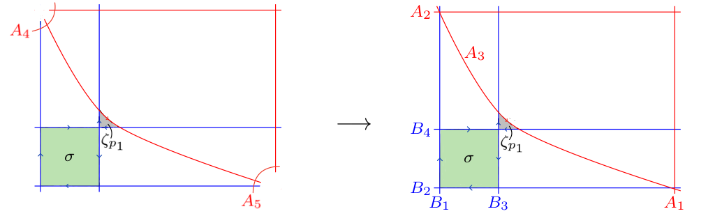
Figure 15. Blowup $X\rightarrow(\mathbb{P}^{1})^{2}$ and divisors $A$ (red) and $B$ (blue) for the dilogarithm (5.8).

When $\lvert t\rvert<1$, the square $[0,1]^{2}$ does not intersect $A$, hence it defines a homology class $\sigma\in H_{2}(Y\setminus A,B)_{t}$ in those fibres. However, the projection

$$\pi\colon Y=(\mathbb{P}^{1})^{3}\longrightarrow T=\mathbb{P}^{1}$$

onto the third factor and the subset $D\subset Y$ are not immediately amenable to Picard-Lefschetz theory, due to two problems:

1. The divisor $A\cup B$ is not normal crossing, e.g. $B_{1}\cap A_{2}\subset A_{3}$.

2. The critical points are not always isolated, e.g. the entire stratum $B_{1}\cap A_{3}\setminus(A_{2}\cup B_{2}\cup B_{4})=\{x_{1}=0\}\times\mathbb{P}^{1}\setminus\{x_{2}=0,1,\infty\}\times\{t=\infty\}$ is contained in a single fibre, so each point on this stratum is critical.

To solve the first problem, we separate the triple intersections by replacing $(\mathbb{P}^{1})^{2}$ with the blow up $X\rightarrow(\mathbb{P}^{1})^{2}$ of the points $(0,\infty),(\infty,0)\in(\mathbb{P}^{1})^{2}$, see fig. 15. We add the exceptional divisors $A_{4,5}$ to the arrangement $\mathfrak{A}$, so that

$$X\setminus\widetilde{A}_{t}\cong(\mathbb{P}^{1})^{2}\setminus A_{t}\quad\text{and}\quad\widetilde{B}\setminus\widetilde{A}\cong B\setminus A$$

where $\widetilde{A}$ is the total transform of $A$ and $\widetilde{B}$ the strict transform of $B$. Having replaced the pair $((\mathbb{P}^{1})^{3}\setminus A,B\setminus A)$ with $(Y\setminus\widetilde{A},\widetilde{B}\setminus\widetilde{A})$, we have achieved that $\widetilde{D}=\widetilde{A}\cup\widetilde{B}$ has normal crossings. Therefore, we can use the canonical stratification of $\widetilde{D}$ to compute the Landau variety. We find $L=\{0,1,\infty\}$:

• Over $t=0$, the quadric $A_{3}$ (we omit $\sim$ in the following) degenerates into a union of two lines, $\{x_{1}=\infty\}\cup\{x_{2}=\infty\}$. Their intersection point $p_{0}=(\infty,\infty,0)\in Y$ would define a quadratic simple pinch, were it not for the fact that these two lines are precisely $A_{1}\cup A_{2}$. Therefore, the critical set over $t=0$ is not just the point $p_{0}$, but rather the entire union

  $$P_{0}\cong(A_{1}\cup A_{2})\cap A_{3}=(A_{1}\cup A_{2})\cap\pi^{-1}(0).$$

• Similarly, the critical set over $t=\infty$ is the union

  $$P_{\infty}\cong(B_{1}\cup B_{2})\cap A_{3}=(B_{1}\cup B_{2})\cap\pi^{-1}(\infty).$$

• Over $t=1$, we have linear simple pinch $p_{1}=(1,1,1)$ at the triple intersection $B_{3}\cap B_{4}\cap A_{3}=\{p_{1}\}$, with vanishing cell $\zeta_{p_{1}}$ (see fig. 15).

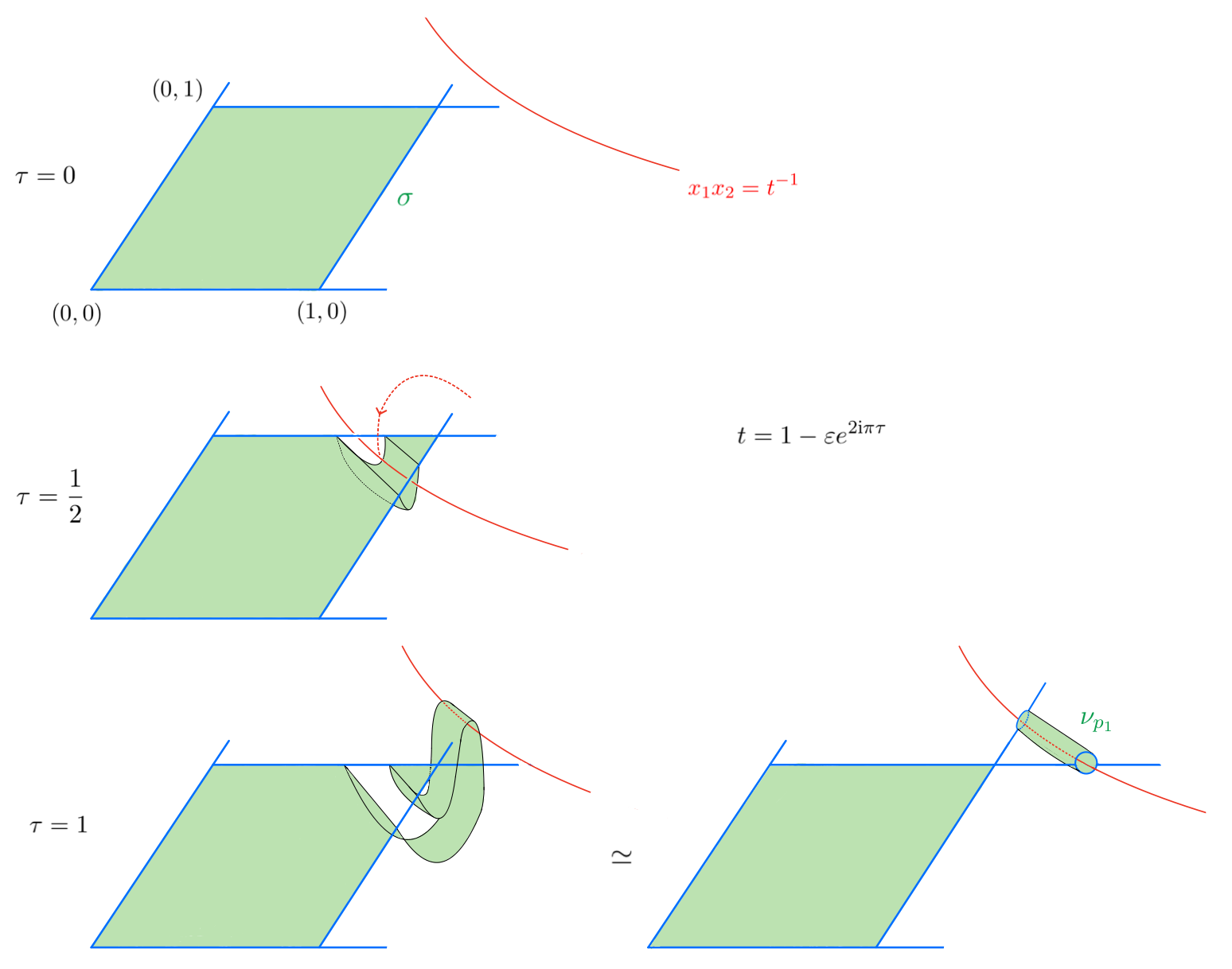
Figure 16. As $t$ encircles the critical value 1, the relative cycle $\sigma=[0,1]^{2}$ is deformed to avoid the quadric $\{x_{1}x_{2}={t}^{-1}\}$. After a full circle, the quadric has “cut out a strip” from $\sigma$, the resulting cycle is now homologous to $\sigma+\nu_{p_{1}}$ (cf. fig. 2).

The Picard-Lefschetz theorem applies only to the linear pinch at $t=1$ (the vanishing cycle is a cylinder, see fig. 16), but not to the non-isolated critical sets over $t=0,\infty$. However, we can still conclude constraints, e.g.

Lemma 5.8.

$\operatorname{Var}_{1}\circ\operatorname{Var}_{0}=\operatorname{Var}_{1}\circ\operatorname{Var}_{1}=\operatorname{Var}_{1}\circ\operatorname{Var}_{\infty}=0$.

Proof.

Consider the terminology from section 4.4. The critical set $P_{0}$ over $t=0$ has type $(\{A_{1},A_{2},A_{3},A_{4},A_{5}\},\{B_{3},B_{4}\})$, because it intersects all divisors except $B_{1,2}$. However, the simple type is just $(\{A_{3}\},\varnothing)$: removing $A_{3}$ from the arrangement makes all critical points disappear, whereas removing any other divisor still leaves critical points behind (especially the quadratic pinch point $p_{0}\in P_{0}$ of $A_{3}$ on its own). So even without an explicit description of $\operatorname{Var}_{0}$, we conclude from 4.12 that it is a coboundary $\delta_{A_{3}}\mu$ of some

(5.9) $$\mu\in H_{1}(A_{3}\setminus(A_{4}\cup A_{5}),B_{3}\cup B_{4})_{t}.$$

Since $p_{1}$ is a linear pinch, the variation at $t=1$ factors through the iterated boundary in $B_{3}$ and $B_{4}$ (3.24). But $A_{3}\cap B_{3}\cap B_{4}\cap\pi^{-1}(t)=\varnothing$ for all $t\neq 1$, so $\partial_{B_{3}}\partial_{B_{4}}\mu\in H_{-1}(A_{3}\cap B_{3}\cap B_{4})_{t}=0$ and thus $\operatorname{Var}_{1}\circ\operatorname{Var}_{0}=0$. A very similar argument shows that $\operatorname{Var}_{1}\circ\operatorname{Var}_{\infty}=0$. Furthermore, $\operatorname{Var}_{1}\circ\operatorname{Var}_{1}=0$ holds for every linear pinch (section 4.2). ∎

Of course, the monodromy of the dilogarithm is well known: with respect to the loops $\gamma_{0}(\tau)=e^{2\mathrm{i}\pi\tau}/2$ and $\gamma_{1}(\tau)=1-\gamma_{0}(\tau)$ based at $t_{0}=1/2$ that generate $\pi_{1}(T\setminus L,t_{0})=\pi_{1}(\mathbb{C}\setminus\{0,1\},t_{0})$, one has

$$\operatorname{Var}_{0}\operatorname{Li}_{2}(t)=0,\quad\operatorname{Var}_{1}\operatorname{Li}_{2}(t)=-2\mathrm{i}\pi\log(t),\quad\operatorname{Var}_{0}\log(t)=2\mathrm{i}\pi.$$

From this, it follows easily that $\operatorname{Var}_{1}\circ\operatorname{Var}_{\ell}\operatorname{Li}_{2}(t)=0$ for $\ell=0,1,\infty$. The point of 5.8 is that such constraints can be derived from purely topological considerations.

Remark 5.9.

Consider the cells $\sigma$ and $\zeta_{p_{1}}$ with the orientation $\mathrm{d}x_{1}\wedge\mathrm{d}x_{2}$, then their intersection in the corner $B_{3}\cap B_{4}=\{(1,1)\}$ gives

$$\operatorname{Var}_{1}\sigma=\langle{\widetilde{\nu}_{p_{1}}}\,|\,{\sigma}\rangle\nu_{p_{1}}=-\langle{\partial_{B_{3}B_{4}}\zeta_{p_{1}}}\,|\,{\partial_{B_{3}B_{4}}\sigma}\rangle\nu_{p_{1}}=-\nu_{p_{1}}$$

by 3.24. So with the additional input $\omega_{t}=\mathrm{d}\log(1-tx_{1}x_{2})\wedge\mathrm{d}\log(x_{1})$ of the actual integrand, Picard-Lefschetz reproduces $\operatorname{Var}_{1}\operatorname{Li}_{2}(t)=-2\mathrm{i}\pi\log(t)$ through the residue theorem (3.10):

$$\int_{\nu_{p_{1}}}\omega_{t}=2\mathrm{i}\pi\int_{\partial_{A_{3}}\zeta_{p_{1}}}\operatorname{Res}_{A_{3}}\omega_{t}=2\mathrm{i}\pi\int_{(1/t,1)}^{(1,1/t)}\mathrm{d}\log(x_{1})=2\mathrm{i}\pi\log(t).$$

Despite the non-isolated critical set $P_{0}$ over $t=0$, the variation $\operatorname{Var}_{0}$ behaves like the variation of the quadratic simple pinch $p_{0}\in A_{3}$, as if the hyperplanes $A_{1}\cup A_{2}$ would not be part of the divisor $D$. Namely, for the quadratic pinch, we would expect that $\operatorname{Var}_{0}h=N(h)\nu_{p_{0}}$ is an integer multiple of the vanishing cycle $\nu_{p_{0}}=\delta_{A_{3}}\eta$, where $\eta\in H_{1}(A_{3}\setminus(A_{4}\cup A_{5}),B_{3}\cup B_{4})_{t}$ is the class of the vanishing sphere $\mathbb{S}^{1}$, embedded as the closed loop

$$\eta(\tau)=(x_{1}(\tau),x_{2}(\tau))=\big{(}e^{2\mathrm{i}\pi\tau}/\sqrt{t},e^{-2\mathrm{i}\pi\tau}/\sqrt{t}\big{)}.$$

The vanishing cycle $\nu_{p_{0}}\in H_{2}(Y\setminus A,B)_{t}$ is the fundamental class of an embedded torus $\mathbb{S}^{1}\!\times\mathbb{S}^{1}\hookrightarrow(\mathbb{P}^{1})^{3}\setminus A$, which we can parametrize explicitly as

$$(x_{1}(\tau,\rho),x_{2}(\tau,\rho))=\big{(}(1+e^{2\mathrm{i}\pi\rho}/2)e^{2\mathrm{i}\pi\tau}/\sqrt{t},\,e^{-2\mathrm{i}\pi\tau}/\sqrt{t}\big{)}.$$

For an isolated quadratic pinch, we also would have $\operatorname{Var}_{0}\circ\operatorname{Var}_{0}=0$ by (4.6).

Lemma 5.10.

For the dilogarithm homology $H_{\bullet}(Y\setminus A,B)_{t}$, the variation $\operatorname{Var}_{0}$ is an integer multiple of $\nu_{p_{0}}$, and $\operatorname{Var}_{0}\circ\operatorname{Var}_{0}=0$.

Proof.

As a quadric in $\mathbb{P}^{1}\!\times\mathbb{P}^{1}$, we have $A_{3}\cap\pi^{-1}(t)\cong\mathbb{P}^{1}$, so the homology group in (5.9) is the group of $\mathbb{P}^{1}$ punctured at two points, relative to two other points. This group has rank 2, generated by a path (in $A_{3}$) from $B_{4}$ to $B_{3}$ ($\partial_{A_{3}}\zeta_{p_{1}}$) and a closed loop ($\eta$). Therefore,

$$\operatorname{Var}_{0}h=N(h)\nu_{p_{0}}+M(h)\nu_{p_{1}}.$$

To see that $M(h)=0$, note that $H_{1}(B_{3}\setminus(A_{2}\cup A_{3}),B_{2}\cup B_{4})_{t}$ has zero variation at $t=0$ (linear pinch of type $(\{A_{2},A_{3}\},\varnothing)$). So $0=\operatorname{Var}_{0}\partial_{B_{3}}h=\partial_{B_{3}}\operatorname{Var}_{0}h=M(h)\alpha$, where the circle $\alpha$ at the $B_{3}$-end of the cylinder $\nu_{p_{1}}$ is non-zero in $H_{1}(B_{3}\setminus(A_{2}\cup A_{3}),B_{2}\cup B_{4})_{t}$. One way to see that $\operatorname{Var}_{0}\nu_{p_{0}}=0$ is to compute $\int_{\nu_{p_{0}}}\omega_{t}=(2\mathrm{i}\pi)^{2}$ with the residue theorem (see 5.9). ∎

Remark 5.11.

The homology classes $\nu_{p_{0}}$, $\nu_{p_{1}}$, and $\sigma$ constitute a basis of $H_{2}(Y\setminus A,B)_{t}\cong\mathbb{Z}^{3}$ at every $t\neq 0,1,\infty$.

6. Feynman integrals

We apply the results of sections 2, 3 and 4 to the study of Feynman integrals in the parametric representation [13, §1]. Such integrals are associated to a graph $G$ (assumed to be connected) with $n+1$ edges $E(G)$, and each edge $e\in E(G)$ labels a coordinate $x_{e}$ (called Schwinger/Feynman parameter) of $X=\mathbb{P}^{n}=\mathbb{P}(\mathbb{C}^{E_{G}})$. The real simplex $\sigma=\{[x_{0}:\cdots:x_{n}]\colon x_{e}>0\}\subset\mathbb{P}^{n}$ defines a relative cycle $\sigma\in H_{n}(X,B)$ with boundary in the divisor

$$B=B_{0}\cup\ldots\cup B_{n},\quad\text{where}\quad B_{e}=\{x_{e}=0\}.$$

The first and second Symanzik polynomials [7] of a graph, $\mathcal{U}\in\mathbb{Z}[x]$ and $\mathcal{F}\in\mathbb{Z}[x,t]$, are homogeneous in $x$ of degrees $h_{1}(G)$ and $h_{1}(G)+1$, respectively. Here $h_{1}(G)=\mathrm{rank}({H_{1}(G)})$ is called the loop number of $G$, and it equals $|E(G)|-|V(G)|+1$ in terms of the number $|V(G)|$ of vertices. We denote the hypersurfaces defined by the Symanzik polynomials as

$$A=A_{1}\cup A_{2},\quad\text{where}\quad A_{1}=\{\mathcal{U}=0\}\quad\text{and}\quad A_{2}=\{\mathcal{F}=0\}.$$

The parameters $t$ in $\mathcal{F}$ have interpretations in physics as masses and scalar products of momenta of particles. These parameters range over a complex variety $T$. We set $Y=X\times T$ and denote $\pi\colon Y\rightarrow T$ the canonical projection.

Definition 6.1.

The Landau variety $L_{G}$ of a Feynman graph $G$ is the minimal (2.9) Landau variety (2.7) of $D=A\cup B\subset Y$.

Our definition follows [12], but other authors [45, 29] use the phrase “Landau variety of $G$” for the subset $L^{\prime}\subseteq L_{G}$ that arises as the Landau variety of the arrangement $A_{2}\cup B$ without $A_{1}$ (so-called first type singularities).

As explained in section 2.4, the Landau variety $L_{G}$ is an upper bound on the singularities of integrals $\mathcal{I}(t)=\int_{\sigma}\omega$, where

(6.1) $$\omega=\frac{P(x,t)\,\Omega}{\mathcal{U}(x)^{D/2-d}\mathcal{F}(x,t)^{d}}\in H_{\mathsf{dR}}^{n}(Y\setminus A,B)$$

is a rational differential $n$-form with poles contained in $A_{1}\cup A_{2}$. The exponents in the denominator are called superficial degree of convergence $d$ and dimension of space-time $D$. We assume that $D/2$ and $d$ are integers, so that $\omega$ is rational and in particular single-valued. The $n$-form

$$\Omega=\sum_{e}(-1)^{e}x_{e}\bigwedge_{k\neq e}\mathrm{d}x_{k}$$

is the projectivized Lebesgue measure, and $P(x,t)$ is a polynomial, homogeneous in $x$ of degree $d-E(G)+h_{1}(G)D/2$, so that $\omega$ is homogeneous of degree zero. The precise form of $P$ is irrelevant for us; it depends on the nature of the particles and interaction vertices encoded by the graph.

To analyse the singularities of an integral $\mathcal{I}(t)=\int_{\sigma}\omega_{t}$ with the topological method (section 2.4), we must in the first step deform the simplex $\sigma$ away from $A$, in order to define a class in $H_{n}(Y\setminus A,B)_{t}$. The resulting integral is then necessarily convergent, and it makes sense to discuss its singularities. We do not consider divergent Feynman integrals; those need to be renormalized first [14].

However, convergence is not sufficient—indeed, it often happens that the boundary of $\sigma$ intersects $A$, so that $\sigma$ cannot define a class in $H_{n}(Y\setminus A,B)_{t}$. This problem is solved by replacing the fibre $\mathbb{P}^{n}$ with an iterated blowup $\rho\colon X\rightarrow\mathbb{P}^{n}$. We will illustrate this construction explicitly in several examples (sections 6.3 and 6.2) and refer to [13] for details. In summary:

• The centres of the blowups are linear subspaces $\bigcap_{e\in\gamma}B_{e}$ indexed by certain subgraphs $\gamma\subset E(G)$, called the motic subgraphs.

• The total transform $\widetilde{B}=\rho^{-1}(B)$ is a simple normal crossings divisor. Its components are (strict transforms of) the original $B_{e}$, plus the exceptional divisors (denoted $B_{\gamma}$, one for each motic subgraph).

• In $X$, the closure $\widetilde{\sigma}=\overline{\rho^{-1}(\sigma\setminus B)}$ of the preimage of the interior of $\sigma$, is a manifold with corners, called the Feynman polytope.

This construction achieves that, for generic parameters $t$ and convergent integrands (6.1), the Feynman polytope and the pullback of $\omega$ define (co)homology classes

$$[\widetilde{\sigma}]\in H_{n}(Y\setminus\widetilde{A},\widetilde{B})_{t}\qquad\text{and}\qquad[\rho^{\ast}\omega]\in H^{n}_{\mathsf{dR}}(Y\setminus\widetilde{A},\widetilde{B})_{t}.$$

Here $\widetilde{A}\subset Y=X\times T$ denotes the strict transform of $A$. We can now indeed apply section 2.4 to study the monodromy of $\mathcal{I}(t)=\int_{\widetilde{\sigma}}\rho^{\ast}\omega$, purely in terms of the homology groups (called the Feynman motive)

(6.2) $$H_{n}(Y\setminus\widetilde{A},\widetilde{B})_{t}=H_{n}(X\setminus\widetilde{A}_{t},\widetilde{B}).$$

To apply our machinery from sections 2 and 3 straightforwardly, we require that $\widetilde{D}=\widetilde{A}\cup\widetilde{B}$ is transverse. Although $\widetilde{B}$ is transverse on its own, this property is easily lost once we add $\widetilde{A}$ to the arrangement. Hence, further blowups become necessary, like for the dilogarithm (section 5.2). There is no general recipe for this step. We will discuss examples where $\widetilde{A}_{2}$ is smooth but not transverse to $\widetilde{B}$ (sections 6.3 and 6.4).

We begin this section with a discussion of the simplest case, massive one loop Feynman integrals. Here, no blowups whatsoever are needed, and all critical points are simple pinches. Hence we can apply the results of sections 3.6, 3.7 and 3.8 and find strong hierarchies according to sections 4.1, 4.2 and 4.3.

After that, we consider two rather degenerate examples: the massive sunrise and the massless triangle (fig. 18). We discuss the construction of their Feynman motives and demonstrate that several Landau singularities arise from non-isolated critical points (section 4.4), and that often the simple type is only $(\{A_{2}\},\varnothing)$. As a consequence, a more subtle analysis is needed to derive hierarchy constraints, and we give examples of such.

In section 6.4 we study the ice cream cone graph and we prove hierarchy constraints in this notoriously subtle case. Note that these subtleties are a general phenomenon rather than an exception, as was already noted in [10]. We suggest a modification of the Feynman motive by additional blowups, to resolve non-transverse intersections (6.14).

6.1. Massive one loop integrals

We consider the geometry associated to generic (fully massive) 1-loop integrals with $n+1$ external and internal edges. The case $n=1$ was discussed in section 1.8.2.

The parameters $t=(m,s)\in T=\mathbb{C}^{(n+1)(n+2)/2}$ consist of $n+1$ masses $m_{i}\in\mathbb{C}$ of internal edges, and $n(n+1)/2$ invariants $s_{ij}=s_{ji}=-(p_{i}+\ldots+p_{j-1})^{2}\in\mathbb{C}$ formed from the incoming momenta $p_{i}\in\mathbb{C}^{D}$ at each vertex. We can identify $T$ with the space of all symmetric $(n+1)\times(n+1)$ matrices $M$, with entries

$$M_{ij}=\begin{cases}m_{i}^{2}&\text{ if }i=j,\\ \frac{m_{i}^{2}+m_{j}^{2}+s_{ij}}{2}&\text{ if }i\neq j.\end{cases}$$

The two Symanzik polynomials are $\mathcal{U}=x_{1}+\ldots+x_{n+1}$ and $\mathcal{F}=x^{\intercal}Mx$. They define a hyperplane $A_{1}=\{\mathcal{U}=0\}$ and a quadric $A_{2}=\{\mathcal{F}=0\}$. Together with the $(n+1)$ coordinate hyperplanes $B_{i}=\{x_{i}=0\}$, we obtain a simple normal crossings divisor $A\cup B\subset\mathbb{P}^{n}\times T$.

The quadric $A_{2t}=A_{1}\cap\pi^{-1}(t)\subset\mathbb{P}^{n}$ is smooth precisely when $\det M\neq 0$. The critical values of $\pi|_{A_{2}}$ form the leading Landau singularity of the first type,

$$\ell_{G}^{\mathcal{F}}=\{\det M=0\}\subset T.$$

Over a generic point $t$ of $\ell_{G}^{\mathcal{F}}$, the rank of $M$ is $n$, and the one-dimensional kernel $\mathbb{C}p$ of $M$ defines the unique singular point $[p]\in\mathbb{P}^{n}$ of $A_{2t}$. This point is a quadratic simple pinch, and the corresponding vanishing cycle is an $\mathbb{S}^{1}$-bundle over the vanishing sphere $\cong\mathbb{S}^{n-1}\subset A_{2t}$ (cf. section 3.5).

The leading singularity of the second type refers to the critical values of the intersection $A_{12}=A_{1}\cap A_{2}$. Its fibre over $t$ is

$$A_{12}\cap\pi^{-1}(t)=\{x_{1}+\ldots+x_{n+1}=0\}\cap\{x^{\intercal}Sx=0\}\subset\mathbb{P}^{n}$$

and depends only on the momentum part $S=M|_{m=0}=(s_{ij}/2)$ of $M$, but not the masses. A point $[x]\in A_{12}$ is critical if either, the normal vectors $\mathbf{1}=(1,\ldots,1)^{\intercal}$ and $Sx$ of $A_{1}$ and $A_{2}$ become collinear, or if $\{x^{\intercal}Sx=0\}$ is singular. So either $\det S=0$, or $S$ is invertible and $x\propto S^{-1}\mathbf{1}$. In the latter case, for $x$ to lie on $A_{12}$, we need $\mathbf{1}^{\intercal}S^{-1}\mathbf{1}=0$. Thus, using the Cayley matrix

$$S^{\prime}=\begin{pmatrix}0&\mathbf{1}^{\intercal}\\ \mathbf{1}&S\\ \end{pmatrix}$$

with determinant $(\mathbf{1}^{\intercal}S^{-1}\mathbf{1})\cdot\det S$, the leading second type singularity is

$$\ell_{G}^{\mathcal{F}\mathcal{U}}=\left\{\det S^{\prime}=0\right\}\subset T.$$

Over a generic point of this component, there is a unique critical point. It is a quadratic simple pinch of type $(\{A_{1},A_{2}\},\varnothing)$. The corresponding vanishing cycle is an $\mathbb{S}^{1}\!\times\mathbb{S}^{1}$-bundle over the vanishing sphere $\cong\mathbb{S}^{n-2}\subset A_{12}\cap\pi^{-1}(t)$.

All other strata lie in $B$. Since $\mathcal{U}|_{x_{e}=0}$ and $\mathcal{F}|_{x_{e}=0}$ are the Symanzik polynomials of the graph $G/e$ where the edge $e$ is contracted, the critical values of $A_{2}\cap B^{I}$ and $A_{12}\cap B^{I}$ are the leading singularities of the quotient graph $G/I$, where $B^{I}=\bigcap_{e\in I}B_{e}$ for any subset $I$ of edges. To summarize:

Proposition 6.2.

The full Landau variety of a generic one-loop graph $G$ is

(6.3) $$L_{G}=\bigcup_{I\subsetneq E(G)}\ell_{G/I}^{\mathcal{F}}\cup\ell_{G/I}^{\mathcal{F}\mathcal{U}}.$$

All components of $L_{G}$ are simple pinch components (3.14).

If we denote by $M_{I}$ and $S^{\prime}_{I}$ the submatrices without the rows and columns indexed by $I$, then $\ell^{\mathcal{F}}_{G/I}=\{\det M_{I}=0\}$ and $\ell^{\mathcal{F}\mathcal{U}}_{G/I}=\{\det S_{I}^{\prime}=0\}$. We exclude $\lvert I\rvert=n+1$ in (6.3) because $B_{1}\cap\ldots\cap B_{n+1}=\varnothing$. In the case $\lvert I\rvert=n$, the graph $G/I$ consists of a single edge, say $i$, and we have no 2nd type singularity: $\ell^{\mathcal{F}\mathcal{U}}_{G/I}=\varnothing$ because $A_{1}\cap B^{I}$ is empty. The first type singularity is

(6.4) $$\ell^{\mathcal{F}}_{G/I}=\{m_{i}^{2}=0\}\quad\text{for}\quad I=E(G)\setminus\{i\}.$$

For $\lvert I\rvert=n-1$, the quotient $G/I$ is a graph with two edges (c.f. section 1.8.2). In particular, the second type singularity is

(6.5) $$\ell_{G/I}^{\mathcal{F}\mathcal{U}}=\{s_{ij}=0\}\quad\text{for}\quad I=E(G)\setminus\{i,j\}.$$

The components (6.4) and (6.5) come from strata that are $(n+1)$-fold intersections, hence linear simple pinches. All other components of $L_{G}$ have quadratic simple pinches.

Figure 17. The hierarchy of the massive triangle integral. An arrow $\ell\rightarrow\ell^{\prime}$ indicates the compatibility $\ell^{\prime}\leqslant\ell$ of the corresponding variations. If there is no directed path from $\ell$ to $\ell^{\prime}$, then $\operatorname{Var}_{\ell^{\prime}}\circ\operatorname{Var}_{\ell}=0$ (section 4.3).

The hierarchy relation defined in section 4 is antisymmetric in this case, and illustrated in eq. 1.5 for $n=1$ and in fig. 17 for $n=2$. The reflexive elements (indicated by a self-loop) are $\ell_{G/I}^{\mathcal{F}}$ with $n-\lvert I\rvert$ odd, and $\ell_{G/I}^{\mathcal{F}\mathcal{U}}$ with $n-\lvert I\rvert$ even, according to (4.6). This hierarchy implies:

1. The variation around a singularity of $G/I$, followed by a variation of a graph $G/J$ that contracts an edge that is not in $I$, must vanish:

   $$\left(\operatorname{Var}_{\ell_{G/J}^{\mathcal{F}\mathcal{U}}}\ \text{or}\ \operatorname{Var}_{\ell_{G/J}^{\mathcal{F}}}\right)\circ\left(\operatorname{Var}_{\ell_{G/I}^{\mathcal{F}\mathcal{U}}}\ \text{or}\ \operatorname{Var}_{\ell_{G/I}^{\mathcal{F}}}\right)=0\quad\text{whenever}\quad J\not\subseteq I.$$

2. The variation of any second type singularity, followed by the variation of any first type singularity, must vanish:

   $$\operatorname{Var}_{\ell_{G/J}^{\mathcal{F}}}\circ\operatorname{Var}_{\ell_{G/I}^{\mathcal{F}\mathcal{U}}}=0\quad\text{for all}\quad I,J\subsetneq E(G).$$

3. If $n-\lvert I\rvert$ is even, then $\operatorname{Var}_{\ell^{\mathcal{F}}_{G/I}}\circ\operatorname{Var}_{\ell^{\mathcal{F}}_{G/I}}=0$. If $n-\lvert I\rvert$ is odd, then $\operatorname{Var}_{\ell^{\mathcal{F}\mathcal{U}}_{G/I}}\circ\operatorname{Var}_{\ell^{\mathcal{F}\mathcal{U}}_{G/I}}=0$.

We hence recover the results of [10, eq.’s (2.7), (2.12–14)]. For an analysis of one-loop integrals in (compactified) momentum space, see [9, 47]. The fundamental group of $T\setminus L$ is studied in [53].

Remark 6.3.

The integrals $\int_{\sigma}\Omega/\mathcal{F}^{D/2}$ with $D=n+1$ compute the volume of a spherical simplex and have been studied in great detail. Since $\mathcal{U}$ is absent, the singularities of 2nd type disappear. It was shown in [1] that these integrals can be written as iterated integrals of logarithmic one-forms. As mentioned in section 5.1, the corresponding symbol encodes the maximal iterated variations. We verified that the symbol [1, eq. (3.15)] is compatible with the hierarchy. In fact, as for the Aomoto polylogarithm, the variations can be computed explicitly using Picard-Lefschetz theory, see [4, §6].

6.2. Massless triangle

Setting a mass to zero is a singularity of the generic one-loop integral. The corresponding linear pinch (6.4) indicates that the integration simplex $\sigma$ now intersects the quadric $A_{2}=\{\mathcal{F}=0\}$ in a corner.

Figure 18. The triangle graph (left) and the sunrise graph (right).

For the massless triangle graph (fig. 18) with parameters $t=(p_{1}^{1},p_{2}^{2},p_{3}^{2})\in T=\mathbb{C}^{3}$ and the Symanzik polynomials

$$\mathcal{U}=x_{1}+x_{2}+x_{3}\quad\text{and}\quad\mathcal{F}=-p_{1}^{2}x_{2}x_{3}-p_{2}^{2}x_{1}x_{3}-p_{3}^{2}x_{1}x_{2},$$

this situation is illustrated in fig. 19. The Feynman motive is obtained from the blowup $X\rightarrow\mathbb{P}^{2}$ of the three intersection points

$$A_{2}\cap B=(B_{2}\cap B_{3})\cup(B_{1}\cap B_{3})\cup(B_{1}\cap B_{2})=\{[1:0:0],[0:1:0],[0:0:1]\}$$

of $B=B_{1}\cup B_{2}\cup B_{3}$. The total transform $\widetilde{B}$ of $B$ includes the exceptional divisors $B_{ij}\cong\mathbb{P}^{1}$ above $x_{i}=x_{j}=0$ and thus has 6 components in total. It bounds the Feynman polytope $\widetilde{\sigma}$, which is a hexagon, see fig. 19.

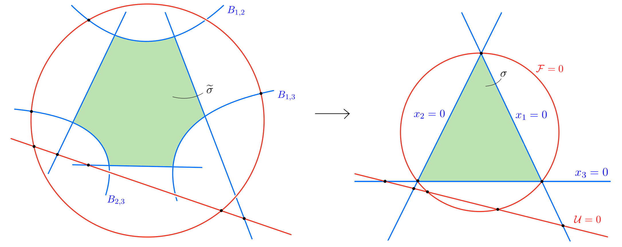
Figure 19. The geometry of the Feynman motive of the massless triangle, in a generic fibre.

The blowups do not affect the existing divisor components, and we denote their strict transforms in $Y=X\times T$ still as $B_{i}$ and $A_{j}$. All divisor components are smooth, $A_{i}\cong B_{j}\cong B_{jk}\cong\mathbb{P}^{1}$, and intersect transversely.

An inspection of the projection $\pi\colon Y\rightarrow T$ and the canonical stratification of $D=A_{1}\cup A_{2}\cup\widetilde{B}$ reveals a Landau variety with 4 components:

(6.6) $$L_{G}=\ell_{1}\cup\ell_{2}\cup\ell_{3}\cup\ell_{\delta}.$$

The first three components $\ell_{i}=\{p_{i}^{2}=0\}$ constitute a singularity of the 1st type. Namely, when $p_{i}^{2}=0$, then $A_{2}\cap Y_{t}=B_{i}\cup\{p_{k}^{2}x_{j}+p_{j}^{2}x_{k}\}$ degenerates into a union of two lines, where $\{i,j,k\}=\{1,2,3\}$. Since one of these lines is $B_{i}$, the critical set over $\ell_{i}$ is not just the simple quadratic pinch point of $A_{2}$ (e.g. $[0:p_{2}^{2}:-p_{3}^{2}]$ for $i=1$), but the entire line $B_{i}$. Note that $A_{2}$ and $B_{i}$ do not intersect for generic $t$, only when $p_{i}^{2}=0$. The critical set over $\ell_{i}$ is therefore not isolated and can be denoted as

$$P_{i}=c(A_{2}\cap B_{i})=B_{i}\cap\ell_{i}=\{x_{i}=0\}\times\{p_{i}^{2}=0\}\subset X\times T.$$

The 2nd type singularity $\ell_{\delta}=\{\delta=0\}$ arises from the coincidence of the two intersection points $(A_{1}\cap A_{2})_{t}=\{Q_{1},Q_{2}\}$. Explicitly, it is defined by

$$\delta=p_{1}^{4}+p_{2}^{4}+p_{3}^{4}-2p_{1}^{2}p_{2}^{2}-2p_{1}^{2}p_{3}^{2}-2p_{2}^{2}p_{3}^{2},$$

because $Q_{1,2}=[-p_{1}^{2}+p_{2}^{2}-p_{3}^{2}\pm\sqrt{\delta}:p_{1}^{2}-p_{2}^{2}-p_{3}^{2}\mp\sqrt{\delta}:2p_{3}^{2}]$ degenerate to the same point when $\delta=0$. This is a quadratic simple pinch, with the vanishing sphere $\{Q_{1},Q_{2}\}\cong\mathbb{S}^{0}$.

The Picard-Lefschetz formula does not apply due to the non-isolated critical set $P_{i}$, but the variation still localizes in the sense of 3.7 into some tubular neighbourhood $W$ of $B_{i}$. The type of $P_{i}$ is $(\{A_{1},A_{2}\},\{B_{i},B_{ij},B_{ik}\})$, but only $A_{2}$ is simple in the sense of 4.9 (c.f. 4.11). So without further analysis, all components of (6.6) have the same simple type, and we do not get any hierarchy constraints from 4.17.

However, with a more detailed analysis, we can (as in 5.8 and 5.10) nevertheless still derive non-trivial constraints:

Lemma 6.4.

$\operatorname{Var}_{\ell_{i}}\circ\operatorname{Var}_{\ell_{i}}=\operatorname{Var}_{\ell_{i}}\circ\operatorname{Var}_{\ell_{\delta}}=0$ for all $i\in\{1,2,3\}$.

Proof.

The type of $P_{i}$ shows that the localization in $W$ factors $\operatorname{Var}_{\ell_{i}}$ through $H_{2}(Y\setminus A,B_{i}\cup B_{ij}\cup B_{ik})_{t}$. Since $A_{2}$ is simple, and $A_{2t}=A_{2}\cap Y_{t}$ does not intersect $B_{i}$, we know that $\operatorname{Var}_{\ell_{i}}$ must be a coboundary $\delta_{A_{2}}$ of some class in

$$H_{1}(A_{2}\setminus A_{1},B_{ij}\cup B_{ik})_{t}\cong\mathbb{Z}^{2}.$$

This group is generated by a path $\gamma_{i}$ in $A_{2t}\setminus A_{1}$ between the points $B_{ij}\cap A_{2t}$ and $B_{ik}\cap A_{2t}$, and a closed loop $\eta=\delta_{A_{1}}Q_{1}=-\delta_{A_{1}}Q_{2}$. Note that

$$\nu_{\delta}=\delta_{A_{2},A_{1}}\partial_{A_{2},A_{1}}\zeta_{\delta}=2\delta_{A_{2}}\delta_{A_{1}}Q_{1}=2\delta_{A_{2}}\eta\in H_{2}(Y\setminus A)_{t}$$

is the vanishing cycle of the quadratic pinch over $\ell_{\delta}$. The image of $\operatorname{Var}_{\ell_{\delta}}$ and $\operatorname{Var}_{\ell_{i}}$ is thus contained in the span of $\nu_{\delta}/2$ and the cylinder

$$\nu_{i}\mathrel{\mathop{:}}=\delta_{A_{2}}\gamma_{i}\in H_{2}(Y\setminus A,B_{ij}\cup B_{ik}\cup B_{jk})_{t}.$$

Since $B_{i}$ is now absent, the critical point over $\ell_{i}$ is an isolated, quadratic simple pinch $q_{i}$ (e.g. $q_{1}=[0:p_{2}^{2}:-p_{3}^{2}]$). The claim, $\operatorname{Var}_{\ell_{i}}\nu_{\delta}=\operatorname{Var}_{\ell_{i}}\nu_{i}=0$, thus follows from the vanishing of the intersection numbers

$$\langle{\zeta_{i}}\,|\,{\nu_{\delta}}\rangle=-2\langle{\partial_{A_{2}}\zeta_{i}}\,|\,{\eta}\rangle\quad\text{and}\quad\langle{\zeta_{i}}\,|\,{\nu_{i}}\rangle=-\langle{\partial_{A_{2}}\zeta_{i}}\,|\,{\gamma_{i}}\rangle$$

with the vanishing cell $\zeta_{i}$ of the quadratic pinch. This cell is localized in a neighbourhood of the critical point $q_{i}$. The intersection with $\nu_{\delta}$ vanishes, because the latter can be localized near $Q_{1}$ or $Q_{2}$, and even over a critical value $t_{c}\in\ell_{i}$ (and hence, by continuity, for nearby $t\notin L$), neither point is equal to $q_{i}$. For example, $q_{1}=[0:p_{2}^{2}:-p_{3}^{2}]$ is not equal to

$$Q_{1}|_{t_{c}}=[0:1:-1]\quad\text{or}\quad Q_{2}|_{t_{c}}=[p_{2}^{2}-p_{3}^{2}:-p_{2}^{2}:p_{3}^{2}],$$

unless $t_{c}$ lies in the intersection $\ell_{1}\cap\ell_{\delta}=\{p_{1}^{2}=0\}\cap\{p_{2}^{2}=p_{3}^{2}\}$.

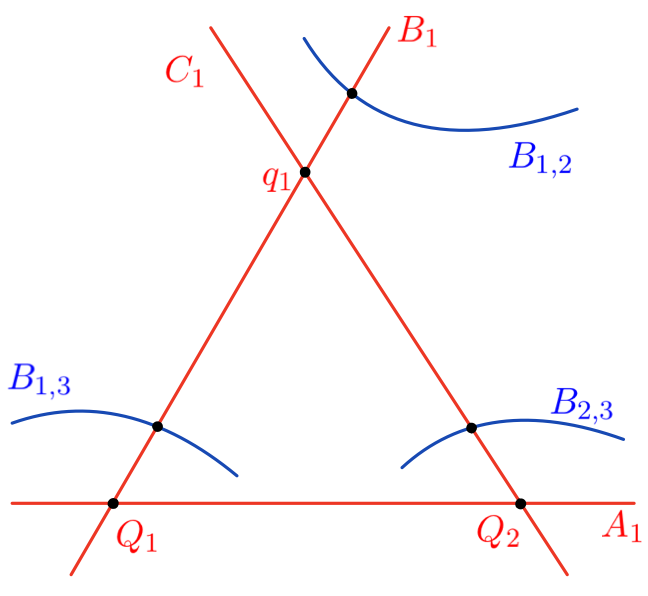
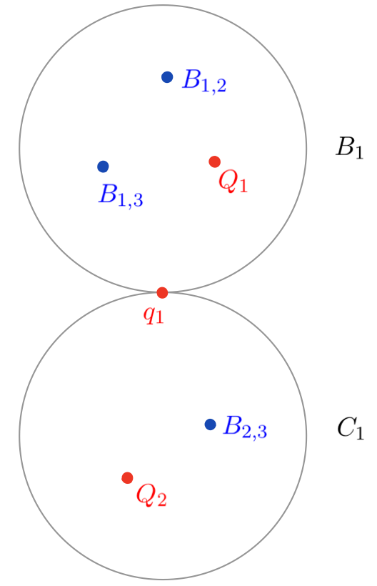
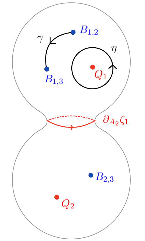
$(A\cup B_{12}\cup B_{13}\cup B_{23})_{t\in\ell_{1}}$	$A_{2}\cap(A_{1}\cap\widetilde{B})_{t\in\ell_{1}}$	$A_{2}\cap(A_{1}\cap\widetilde{B})_{t\notin\ell_{1}}$

Figure 20. The reduced divisor (without $B$) of the massless triangle in a critical fibre (left), the degenerate quadric $A_{2t}=B_{1}\cup C_{1}$ (middle), the quadric $A_{2t}$ in a nearby fibre (right).

The embedded vanishing sphere $\mathbb{S}^{1}\subset A_{2t}$ with class $[\mathbb{S}^{1}]=\partial_{A_{2}}\zeta_{i}$ cuts the quadric $A_{2t}\cong\mathbb{S}^{2}$ over $t\notin L$ into two hemispheres. Over $\ell_{i}$, these hemispheres degenerate into the two components $B_{i}$ and $C_{i}=\{p_{k}^{2}x_{j}+p_{j}^{2}x_{k}=0\}$ of $A_{2t_{c}}$. Since both endpoints of $\gamma_{i}$ lie on the same component ($B_{i}$) in the critical fibre, they must lie on the same hemisphere for $t$ near, but not on, $\ell_{i}$. Hence the path $\gamma_{i}$ can be homotoped to lie within that hemisphere and thus does not intersect the vanishing sphere. This is illustrated in fig. 20. ∎

In summary, for the massless triangle, the double variations can be computed using Picard-Lefschetz theory: after the first variation, no cycle has boundary in $B$, hence we can drop $B$ from the arrangement such that for the second variation, the critical points are quadratic simple pinches.

6.4 covers all constraints of the form $\operatorname{Var}_{\ell^{\prime}}\circ\operatorname{Var}_{\ell}=0$. In particular,

(6.7) $$\operatorname{Var}_{\ell_{i}}\circ\operatorname{Var}_{\ell_{j}}\neq 0$$

for distinct $i,j\in\{1,2,3\}$. Namely, $\langle{\zeta_{i}}\,|\,{\nu_{j}}\rangle=\pm 1$ and so $\operatorname{Var}_{\ell_{i}}\nu_{j}=\pm\nu_{\delta}/2$. Furthermore, although this does not follow directly from Picard-Lefschetz theory, we can choose $\gamma_{i}$ so that $\operatorname{Var}_{\ell_{i}}\widetilde{\sigma}=\nu_{i}$, and therefore

$$\operatorname{Var}_{\ell_{i}}\circ\operatorname{Var}_{\ell_{j}}\widetilde{\sigma}=\pm\nu_{\delta}/2.$$

Remark 6.5.

If one interprets $\operatorname{Var}_{\ell_{i}}$ as only the singularity of the massless bubble quotient graph $G/i$, then (6.7) would violate the hierarchy principle of absorption integrals [49, 29]. However, there is no contradiction here, because the latter does not apply to Feynman integrals to begin with (the integration domain $\widetilde{\sigma}$ has boundary), and also because the masses would be required to be non-zero. In addition, the Landau components $\ell_{i}$ also parametrize the leading singularity of the full triangle graph, hence $\operatorname{Var}_{\ell_{i}}$ cannot be attributed to $G/i$ alone (in our terminology, $B_{i}$ is not simple).

Remark 6.6.

The relations from 6.4 and (6.7) agree with explicit computations of the triangle integral in terms of polylogarithms [8, §6.2.2].

6.3. Massive sunrise

The sunrise graph with unequal masses depends on four parameters $t=(p^{2},m_{1},m_{2},m_{3})\in T=\mathbb{C}^{4}$. Its Symanzik polynomials

$$\mathcal{U}=x_{2}x_{3}+x_{1}x_{3}+x_{1}x_{2},\quad\mathcal{F}=(m_{1}^{2}x_{1}+m_{2}^{2}x_{2}+m_{3}^{2}x_{3})\mathcal{U}-p^{2}x_{1}x_{2}x_{3}$$

define a smooth quadric and cubic, respectively, in $\mathbb{P}^{2}$. Both of them intersect in the corners $x_{i}=x_{j}=0$ of the simplex $\{x_{1}x_{2}x_{3}=0\}$. The Feynman motive is defined by the same blowup $X^{\prime}\rightarrow\mathbb{P}^{2}$ as in section 6.2. It achieves the separation of the hexagon $\widetilde{\sigma}$ (Feynman polytope), which has boundary in

$$B^{\prime}=B^{\prime}_{1}\cup B^{\prime}_{2}\cup B^{\prime}_{3}\cup B^{\prime}_{12}\cup B^{\prime}_{13}\cup B^{\prime}_{23},$$

from the strict transforms $A_{1}^{\prime},A_{2}^{\prime}\subset X^{\prime}\times T$ of $\{\mathcal{U}=0\}$ and $\{\mathcal{F}=0\}$. Here we denote $B_{i}^{\prime}$ the strict transform of $\{x_{i}=0\}$ and $B^{\prime}_{ij}$ the exceptional divisors over the points $\{x_{i}=x_{j}=0\}\in\mathbb{P}^{2}$.

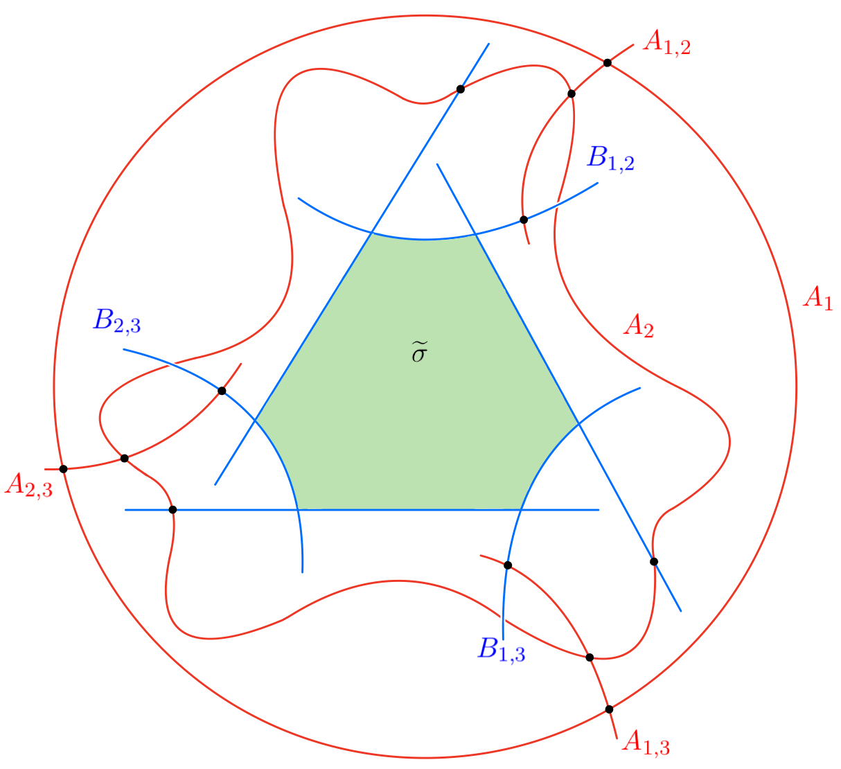
$\subset X\quad\longrightarrow\quad X^{\prime}\supset$

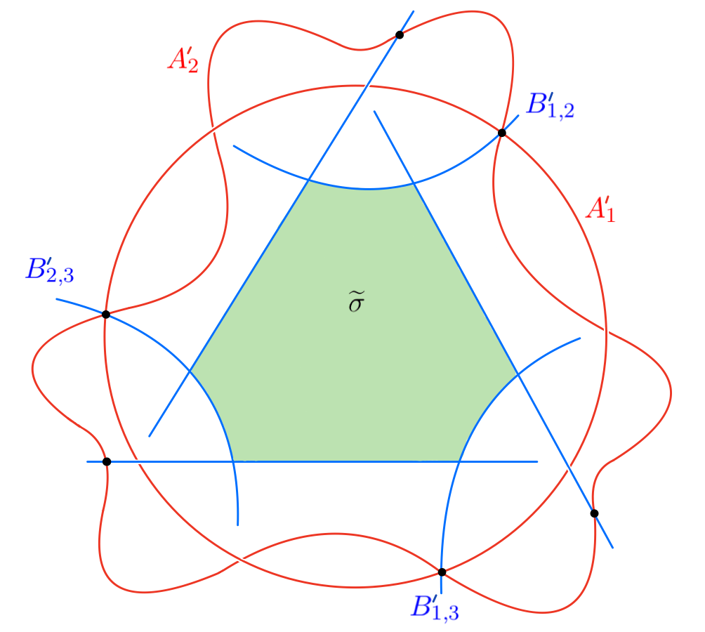
Figure 21. Divisors $A\cup B\subset X$ and $A^{\prime}\cup B^{\prime}\subset X^{\prime}$ of the sunrise graph.

However, the divisor $A^{\prime}\cup B^{\prime}\subset X^{\prime}\times T$ is still not normal crossing, because on each $B^{\prime}_{ij}$, the intersections with $A_{1}^{\prime}$ and $A_{2}^{\prime}$ coincide (see fig. 21). For example, in local coordinates $x=[u:uv:1]$ where $B^{\prime}_{12}=\{u=0\}$, one finds

$$A_{1}^{\prime}\cap B^{\prime}_{12}=A_{2}^{\prime}\cap B^{\prime}_{12}=\{v=-1\}\subset B^{\prime}_{12}.$$

This is resolved by an additional blowup $X\rightarrow X^{\prime}$ of the fibre in the three points $A_{1}^{\prime}\cap B^{\prime}_{ij}$. Let $A_{ij}$ denote the corresponding exceptional divisors, and write $A_{i}$, $B_{i}$, $B_{ij}$ for the strict transforms of $A_{i}^{\prime}$, $B_{i}^{\prime}$, and $B_{ij}^{\prime}$. We set

$$A=A_{1}\cup A_{2}\cup A_{12}\cup A_{13}\cup A_{23}$$

and analyse the normal crossings divisor $A\cup B\subset Y=X\times T$ with respect to the projection $\pi\colon Y\to T$. This is illustrated in fig. 21. Note in particular that, in a generic fibre, $A_{1}$ and $A_{2}$ do not intersect.

Lemma 6.7.

Let $\ell_{p}=\{p^{2}=0\}$, $\ell_{i}=\{m_{i}^{2}=0\}$ for $i\in\{1,2,3\}$, and for any pair of signs $\alpha,\beta\in\{1,-1\}$ set $\ell_{\alpha\beta}=\{p^{2}=(m_{1}+\alpha m_{2}+\beta m_{3})^{2}\}$.

The Landau variety of the sunrise graph is

$$L_{G}=\ell_{p}\cup\ell_{1}\cup\ell_{2}\cup\ell_{3}\cup\ell_{++}\cup\ell_{+-}\cup\ell_{-+}\cup\ell_{--}.$$

Proof.

The Landau variety contains in particular the critical values of the cubic $A_{2}$. Those are determined by the parameters $t$ such that the fibre $A_{2t}=A_{2}\cap\pi^{-1}(t)$ is singular. This discriminant of $\mathcal{F}$ is

$$p^{2}m_{1}^{2}m_{2}^{2}m_{3}^{2}\prod_{\alpha,\beta=\pm}\big{(}p^{2}-(m_{1}+\alpha m_{2}+\beta m_{3})^{2}\big{)}$$

and produces $L_{G}$. It remains to verify that the intersections of $A_{2}$ with (one or several) of the other components $A_{1},A_{ij},B_{i},B_{ij}$ do not generate additional components. This is a routine calculation. ∎

In order to describe the variations, we need to determine the critical sets $P\subset\pi^{-1}(t_{c})$ over a generic critical value $t_{c}\in L$. These are as follows:

• Over $\ell_{\alpha\beta}$, $P$ is a quadratic simple pinch of type $(\{A_{2}\},\varnothing)$. This point is the unique node (double point) of the cubic $A_{2t}$. In coordinates:

  $$P=\{[\alpha\beta m_{2}m_{3}:\beta m_{1}m_{3}:\alpha m_{1}m_{2}]\}.$$

• Over $\ell_{i}$, the cubic $A_{2t}$ acquires two nodes and splits into two $\mathbb{P}^{1}$. For example, in the chart $x=[u:uv:1]$ with $B_{12}=\{u=0\}$,

  $$A_{2t}\cap B_{12}=\{(1+v)m_{3}^{2}=0\}$$

  is generically a point; but for $t_{c}\in\ell_{3}$, it contains the entire hyperplane $B_{12}\subset A_{2t_{c}}$. The other factor of $A_{2t_{c}}$ (solve $\mathcal{F}$ for $x_{3}$) is the image of

  $$\mathbb{P}^{1}\ni[y_{1}:y_{2}]\mapsto\left[y_{1}:y_{2}:\tfrac{y_{1}y_{2}(m_{1}^{2}y_{1}+m_{2}^{2}y_{2})}{p^{2}y_{1}y_{2}-(y_{1}+y_{2})(m_{1}^{2}y_{1}+m_{2}^{2}y_{2})}\right].$$

  The two components of $A_{2t_{c}}$ meet in the two roots $v=y_{2}/y_{1}$ of $p^{2}v=(1+v)(m_{1}^{2}+m_{2}^{2}v)$. These double points are quadratic simple pinches of $A_{2}$; however, since the factor $B_{12}$ is in the arrangement, the critical set is not isolated:

  $$P=B_{jk}\cap\pi^{-1}(t_{c})\quad\text{with type}\quad(\{A_{1},A_{2},A_{jk}\},\{B_{j},B_{k},B_{jk}\}).$$

• Over $t_{c}\in\ell_{p}$, the cubic also degenerates into two components, $A_{2t_{c}}=(A_{1}\cup\{x_{1}m_{1}^{2}+x_{2}m_{2}^{2}+x_{3}m_{3}^{2}=0\})_{t_{c}}$. These components intersect in two quadratic simple pinches of $A_{2}$, and the critical set is

  $$P=A_{1}\cap\pi^{-1}(t_{c})\quad\text{with type}\quad(\{A_{1},A_{2},A_{12},A_{13},A_{23}\},\varnothing).$$

The simple type of every critical set is just $(\{A_{2}\},\varnothing)$, because the divisor $A_{2}\subset Y$ alone already produces the entire Landau variety. As for the massless triangle, we thus get no hierarchy constraints from 4.17, at least not between different variations. For the simple pinches, we do get that

(6.8) $$\operatorname{Var}_{\ell_{\alpha\beta}}\circ\operatorname{Var}_{\ell_{\alpha\beta}}=0$$

for all $\alpha,\beta\in\{1,-1\}$, from (4.6). Furthermore, with a very similar argument as in the proof of 6.4, one can show that

(6.9) $$\operatorname{Var}_{\ell_{i}}\circ\operatorname{Var}_{\ell_{i}}=0$$

for all $i\in\{1,2,3\}$. Note in particular that, by the localization near the critical set, the variations of any class $h\in H_{2}(Y\setminus A,B)_{t}$ take values in

$$\operatorname{Var}_{\ell_{\alpha\beta}}h,\operatorname{Var}_{\ell_{p}}h \in\delta_{A_{2}}H_{1}(A_{2}\setminus(A_{12}\cup A_{13}\cup A_{23}),\varnothing)_{t}\quad\text{and}$$

$$\operatorname{Var}_{\ell_{i}}h \in\delta_{A_{2}}H_{1}(A_{2}\setminus(A_{12}\cup A_{13}\cup A_{23}),B_{j}\cup B_{k})_{t}.$$

So after any first variation, no cycle has boundary in $B_{12}\cup B_{13}\cup B_{23}$, so we can drop those from the arrangement. Thus the critical points over $\ell_{i}$ for the second variation are just the two nodes, hence subject to the Picard-Lefschetz theorem, and we can proceed as in 6.4 to confirm (6.9).

6.4. Ice cream cone

  

Figure 22. The ice cream cone $G$, the subgraph $\gamma=\{1,2\}$, and the quotient graph $G/\gamma$.

The graph $G$ with four edges in fig. 22 depends on seven parameters $t=(p_{1}^{2},p_{2}^{2},p_{3}^{2},m_{1},m_{2},m_{3},m_{4})\in T=\mathbb{C}^{7}$. The Symanzik polynomials are

$$\mathcal{U} =x_{1}x_{2}+(x_{1}+x_{2})(x_{3}+x_{4})\quad\text{and}$$

$$\mathcal{F} =x_{1}x_{2}(-p_{2}^{2}x_{4}-p_{3}^{2}x_{3})-p_{1}^{2}(x_{1}+x_{2})x_{3}x_{4}+\mathcal{U}\sum_{1\leq i\leq 4}m_{i}^{2}x_{i}.$$

The Feynman motive is obtained from the blowup $X^{\prime}\rightarrow\mathbb{P}^{3}$ in the two points $\{[0:1:0:0],[1:0:0:0]\}$ and the line $\{x_{1}=x_{2}=0\}$. Its boundary divisor $B^{\prime}$ has 7 components: exceptional divisors $B^{\prime}_{134}$, $B^{\prime}_{234}$, $B^{\prime}_{12}$ and strict transforms $B^{\prime}_{i}$ of $\{x_{i}=0\}$. The strict transforms $A_{1}^{\prime}$ and $A_{2}^{\prime}$ of $\{\mathcal{U}=0\}$ and $\{\mathcal{F}=0\}$ are smooth surfaces in $Y^{\prime}=X^{\prime}\times T$. The Feynman polytope (fig. 23) has facets in all 7 components of $B^{\prime}$ and defines a class

Figure 23. The Feynman polytope $\widetilde{\sigma}$ of the ice cream cone.

$$\widetilde{\sigma}\in H_{3}(Y^{\prime}\setminus A^{\prime},B^{\prime})_{t}.$$

Although $B^{\prime}$ is transverse and all components of $D^{\prime}=A^{\prime}\cup B^{\prime}$ are smooth, the arrangement $D^{\prime}$ is not transverse. In particular, $A_{1}^{\prime}$ and $A_{2}^{\prime}$ are not transverse to $B_{12}^{\prime}$, because the intersections $A_{1}^{\prime}\cap B_{12}^{\prime}$ and $A_{2}^{\prime}\cap B_{12}^{\prime}$ are singular: Note that in coordinates $x=[u:uv:x_{3}:1]$, the divisor

(6.10) $$B_{12}^{\prime}=\{u=0\}=\{([1:v],[x_{3}:1]\}=\mathbb{P}^{1}\times\mathbb{P}^{1}$$

is canonically identified with the product of the coordinates $[1:v]=[x_{1}:x_{2}]$ of the subgraph $\gamma=\{1,2\}$ and $[x_{3}:x_{4}]$ of the quotient graph $G/\gamma$. The Symanzik polynomials vanish to first order on $B_{12}^{\prime}$, with

(6.11) $$\mathcal{U} \equiv\mathcal{U}_{\gamma}\mathcal{U}_{G/\gamma}\equiv(x_{1}+x_{2})(x_{3}+x_{4})\quad\text{and}$$

$$\mathcal{F} \equiv\mathcal{U}_{\gamma}\mathcal{F}_{G/\gamma}\equiv(x_{1}+x_{2})(-p_{1}^{2}x_{3}x_{4}+(x_{3}+x_{4})(m_{3}^{2}x_{3}+m_{4}^{2}x_{4}))$$

modulo terms of order $u^{2}$ or higher. The factorization of the leading order in $u$ into Symanzik polynomials of $\gamma$ and $G/\gamma$ is well-known [13]. Therefore,

$$A_{1}^{\prime}\cap B_{12}^{\prime} =\{[1:-1]\}\times\mathbb{P}^{1}\cup\mathbb{P}^{1}\times\{[1:-1]\}\quad\text{and}$$

$$A_{2}^{\prime}\cap B_{12}^{\prime} =\{[1:-1]\}\times\mathbb{P}^{1}\cup\mathbb{P}^{1}\times\{\mathcal{F}_{G/\gamma}=0\}$$

are unions of lines (fig. 24). In a generic fibre, they have three singularities, the intersection points $\{[1:-1]\}\times\{[1:-1],Q_{1},Q_{2}\}$ where $Q_{1,2}\in\mathbb{P}^{1}$ denote the roots of $\mathcal{F}_{G/\gamma}=0$. Note also that $A_{1}^{\prime}\cap A_{2}^{\prime}\cap B_{12}^{\prime}=\{[1:-1]\}\times\mathbb{P}^{1}$ intersect not in a point but in a line—another witness of non-transversality.

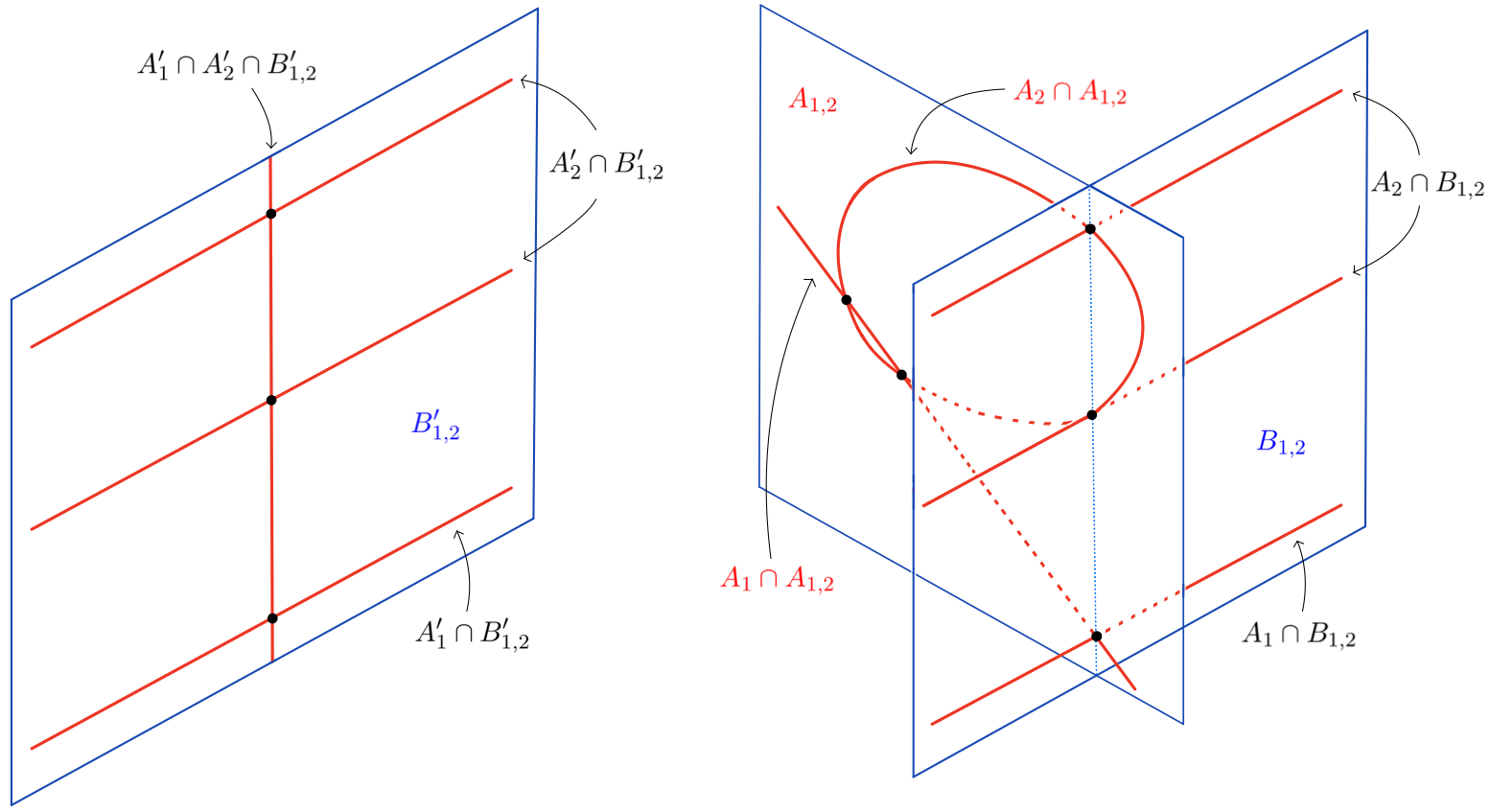
Figure 24. Singular intersection $A^{\prime}\cap B_{12}^{\prime}$ (left) and transverse arrangement $A\cup B_{12}$ (right) after blowup.

Similarly, we identify two further non-transverse intersections. Instead of a point, $A_{1}^{\prime}\cap A_{2}^{\prime}\cap B_{134}^{\prime}\cong\mathbb{P}^{1}$ intersect in the line

$$\{\mathcal{U}_{134}=0\}=\{x_{1}+x_{3}+x_{4}=0\}\subset B_{134}^{\prime}\cong\mathbb{P}^{2},$$

and analogously for $B_{234}^{\prime}$. To rectify all these problems, we make

Definition 6.8.

We define the fibre $X$ of the ice cream cone as the blowup $X\rightarrow X^{\prime}$ of the Feynman motive $X^{\prime}$ in the three lines (each is $\cong\mathbb{P}^{1}$)

(6.12) $$\{\mathcal{U}_{12}=0\}\subset B_{12}^{\prime},\ \{\mathcal{U}_{134}=0\}\subset B_{134}^{\prime},\ \{\mathcal{U}_{234}=0\}\subset B_{234}^{\prime}.$$

We denote the corresponding exceptional divisors as $A_{12}$, $A_{134}$, $A_{234}$ and otherwise write $A_{\bullet}$, $B_{\bullet}$ for the strict transforms of $A_{\bullet}^{\prime}$ and $B_{\bullet}^{\prime}$. We set $Y=X\times T$ and obtain a divisor $A\cup B\subset Y$.

Remark 6.9.

The component $B_{3}^{\prime}$ is the blowup of $\mathbb{P}^{2}\cong\{x_{3}=0\}\subset\mathbb{P}^{3}$ in the 3 corners of $\{x_{1}x_{2}x_{4}=0\}$. This is precisely the fibre denoted $X^{\prime}$ in section 6.3, corresponding to the quotient sunrise graph $G/3$. Each of the 3 lines (6.12) intersects $B_{3}^{\prime}$ in a point, so $B_{3}$ is the blowup of $B_{3}^{\prime}$ in 3 further points, that is, $B_{3}$ is isomorphic to the fibre denoted $X$ in section 6.3. This means that the operadic structure of Feynman motives $X^{\prime}$ from [13] extends to the spaces $X\rightarrow X^{\prime}$ with our additional blowups.

Lemma 6.10.

The divisor $D=A\cup B\subset Y$ has simple normal crossings.

Proof.

In coordinates $x=[u:uv:x_{3}:1]$ where $B_{12}^{\prime}=\{u=0\}$, we are blowing up $\{u=0\}\cap\{v=-1\}$. Hence in the chart $x=[\lambda w:\lambda w(\lambda-1):x_{3}:1]$, we see $B_{12}=\{w=0\}$ and $A_{12}=\{\lambda=0\}$. The strict transform

$$A_{1}=\{1+x_{3}-w+w\lambda=0\}$$

intersects $B_{12}$ in the horizontal line $\{x_{3}=-1\}$, whereas the previously vertical line has moved onto $A_{12}\cap A_{1}=\{w=1+x_{3}\}$. In the same coordinates, the strict transform $A_{2}$ of $A_{2}^{\prime}$ reads

$$0=-p_{1}^{2}x_{3}+(1+x_{3}-w)(m_{3}^{2}x_{3}+m_{4}^{2})+w(p_{2}^{2}+x_{3}p_{3}^{2})+w\lambda\cdot(\cdots).$$

We see that $A_{2}\cap B_{12}$ is smooth, namely the union of two non-intersecting lines (parametrized by $\lambda$) with $w=0$ and $x_{3}$ a root of $\mathcal{F}_{G/\gamma}$. The other intersection is also smooth, namely the quadric

(6.13) $$A_{2t}\cap A_{12}=\{\lambda=0\}\cap\{w(m_{3}^{2}x_{3}+m_{4}^{2}-p_{2}^{2}-p_{3}^{2}x_{3})=\mathcal{F}_{G/\gamma}\}\cong\mathbb{P}^{1}.$$

This geometry is illustrated in fig. 24. Similarly, one can verify the transversality of $D$ near $A_{134}$, $B_{134}$, $A_{234}$, and $B_{234}$. ∎

Since we blow up subsets of $A_{2}^{\prime}$, these blowups do not change the complements $Y\setminus A\cong Y^{\prime}\setminus A^{\prime}$ and thus we have a canonical identification

$$H_{3}(Y\setminus A,B)_{t}=H_{3}(Y^{\prime}\setminus A^{\prime},B^{\prime})_{t}.$$

Because $A\cup B$ has normal crossings, we can now apply our results and analyse the Landau variety and variation constraints using the canonical stratification of $A\cup B$. Instead of a complete analysis, we discuss two particularly interesting cases, stemming from only 3 components of $D$:

$$A_{2}\cup A_{12}\cup B_{12}.$$

In physics language, the critical values of $A_{2}\cup A_{12}$ would be called leading singularities (absence of boundary $B$) of first type (absence of $A_{1}$). They constitute singularities of integrals $\int_{\sigma}\omega_{t}$ where $\sigma\in H_{3}(Y\setminus(A_{12}\cup A_{2}),\varnothing)_{t}$ has no boundary, and the integrand $\omega$ has only $\mathcal{F}$ in the denominator (no $\mathcal{U}$). Note that $\mathcal{F}$ vanishes on $A_{12}$, hence we cannot discard $A_{12}$ (the differential form $\omega$ can have poles on $A_{12}$). Critical values of $B_{12}\cap A_{2}$ might be called reduced singularities, associated with the quotient graph $G/\gamma$. Instead, we will use the terminology of type and simple type (section 4.4).

In the coordinates $(w,x_{3})$ on $A_{12}$ from the proof of 6.10, the singular points of the quadric (6.13) constitute the critical set

(6.14) $$c(A_{2}\cap A_{12})=\Big{\{}w=\frac{\partial_{x_{3}}\mathcal{F}_{G/\gamma}}{m_{3}^{2}-p_{3}^{2}}\Big{\}}\cap\Big{\{}x_{3}=-\frac{m_{4}^{2}-p_{2}^{2}}{m_{3}^{2}-p_{3}^{2}}\Big{\}}\cap\Big{\{}\mathcal{F}_{G/\gamma}=0\Big{\}}.$$

This set has a non-empty fibre only when $x_{3}=-(m_{4}^{2}-p_{2}^{2})/(m_{3}^{2}-p_{3}^{2})$ is a root of $\mathcal{F}_{G/\gamma}$ from (6.11). The corresponding discriminant defines a component $\ell_{A_{12}}\subset L_{G}$ of the Landau variety, concretely

(6.15) $$\ell_{A_{12}}=\big{\{}p_{1}^{2}(m_{3}^{2}-p_{3}^{2})(m_{4}^{2}-p_{2}^{2})+(m_{3}^{2}p_{2}^{2}-m_{4}^{2}p_{3}^{2})(m_{3}^{2}-m_{4}^{2}+p_{2}^{2}-p_{3}^{2})=0\big{\}}.$$

Over a generic point $t$ of $\ell_{A_{12}}$, the critical point (6.14) is not a critical point for $A_{2}$, that is, $A_{2t}$ remains smooth over $\ell_{A_{12}}$. This means that the type and simple type of $\ell_{A_{12}}$ are the same: $(\{A_{12},A_{2}\},\varnothing)$. More precisely, (6.14) is a quadratic simple pinch, where $A_{2}\cap A_{12}$ degenerates into two lines,

(6.16) $$A_{2t}\cap A_{12}=\Big{\{}x_{3}=-\frac{m_{4}^{2}-p_{2}^{2}}{m_{3}^{2}-p_{3}^{2}}\Big{\}}\cup\Big{\{}w=\frac{m_{3}^{2}x_{3}}{m_{3}^{2}-p_{3}^{2}}+\frac{m_{4}^{2}}{m_{4}^{2}-p_{2}^{2}}\Big{\}}.$$

Now consider the submanifold $A_{2}\cap B_{12}=\mathbb{P}^{1}\times\{\mathcal{F}_{G/\gamma}=0\}$. In a generic fibre, it consists of two lines (coordinate $\lambda=v+1$), which degenerate into a single line when the two roots of $\mathcal{F}_{G/\gamma}$ coincide. Hence, the corresponding contribution $\ell_{B_{12}}\subset L_{G}$ to the Landau variety of the ice cream cone is

(6.17) $$\ell_{B_{12}}=\ell^{\mathcal{F}}_{G/\gamma}=\{p_{1}^{2}=(m_{3}\pm m_{4})^{2}\}$$

in the notation from section 6.1, the leading singularity of the bubble graph $G/\gamma$ (section 1.8.2). The critical set over $t\in\ell_{B_{12}}$ is not isolated:

$$c(A_{2}\cap B_{12})\cap\pi^{-1}(t)=\mathbb{P}^{1}\times\big{\{}[x_{3}:x_{4}]=[m_{4}:\pm m_{3}]\big{\}}.$$

This line intersects also $B_{1}=\{\lambda=\infty\}$, $B_{2}=\{\lambda=1\}$ and $A_{12}=\{\lambda=0\}$. The component $B_{12}$ is not simple over $t\in\ell_{B_{12}}$, because two points

(6.18) $$c(A_{2})\cap\pi^{-1}(t)=\{P_{1},P_{2}\}\times\{[m_{4}:\pm m_{3}]\}\subset c(A_{2}\cap B_{12})$$

on this line are critical points of $A_{2}$ alone. This fact, that $B_{12}$ is not simple for the singularity $\ell_{B_{12}}$, was noted already in [10, §4] and [36, §2].

Corollary 6.11.

The bubble singularity (6.17) of the ice cream cone graph has type $(\{A_{2},A_{12}\},\{B_{1},B_{2},B_{12}\})$ and simple type $(\{A_{2}\},\varnothing)$. The type and simple type of the singularity (6.15) is $(\{A_{2},A_{12}\},\varnothing)$.

Let $\mathfrak{L}_{G}$ denote the codimension one components of the full Landau variety $L_{G}$ of the ice cream cone $G$, and $\mathfrak{L}_{G/\gamma}$ correspondingly for the bubble quotient. Note that $\mathfrak{L}_{G/\gamma}\subset\mathfrak{L}_{G}$. If $B_{12}$ were simple for $\ell_{B_{12}}$, then section 4 would give

(6.19) $$\operatorname{Var}_{\ell_{B_{12}}}\circ\operatorname{Var}_{\ell}=0\quad\text{for all}\quad\ell\in\mathfrak{L}_{G}\setminus\mathfrak{L}_{G/\gamma}.$$

Namely, a compatible variation requires that $\ell$ has $B_{12}$ in its type, meaning that the critical set $P$ over $\ell$ intersects $B_{12}$, and thus $P\cap B_{12}$ are critical points of $B_{12}$—showing that the restriction of the arrangement $A\cup B$ to $B_{12}$ is critical over $\ell$ (hence $\ell\in\mathfrak{L}_{G/\gamma}$). Anyway, $B_{12}$ is not simple, and indeed, (6.19) does not hold [36, eq. (14)].

However, we do have hierarchy constraints in the $\mathfrak{A}$-direction:

(6.20) $$\operatorname{Var}_{\ell}\circ\operatorname{Var}_{\ell_{A_{12}}}=0,$$

unless $\ell$ has $A_{12}$ and $A_{2}$ in its type. In fact, since $\ell_{A_{12}}$ is a simple pinch component, its vanishing cycle is an iterated coboundary $\nu=\delta_{A_{2}}\delta_{A_{12}}\eta$ around the vanishing sphere

(6.21) $$\eta=\partial_{A_{12}}\partial_{A_{2}}\zeta=[\mathbb{S}^{1}]\in H_{1}(A_{2}\cap A_{12}\setminus A_{1})_{t}\cong\mathbb{Z}.$$

This group has rank one, because $A_{2t}\cap A_{12}\cong\mathbb{P}^{1}$ from (6.13) is punctured in two points $A_{2t}\cap A_{12}\cap A_{1}=\{R_{1},R_{2}\}$. The vanishing sphere $\eta$ separates the two punctures, because over the critical fibre, the line $A_{1}\cap A_{12}$ intersects each of the two components (6.16) once. Therefore, $\eta=\delta_{R_{1}}1=-\delta_{R_{2}}1$ is a generator of (6.21).

By (4.6), $\operatorname{Var}_{\ell_{A_{12}}}\nu=0$. The only other singularity of $A_{2}\cap A_{12}\setminus A_{1}$ is the quadratic simple pinch of $A_{2}\cap A_{12}\cap A_{1}$, when $R_{1}=R_{2}$. This happens over a singularity $\ell_{\delta}\in\mathfrak{L}_{G}$ that is familiar from the triangle graph:

(6.22) $$\ell_{\delta}=\big{\{}p_{1}^{4}+p_{2}^{4}+p_{3}^{4}-2p_{1}^{2}p_{2}^{2}-2p_{1}^{2}p_{3}^{2}-2p_{2}^{2}p_{3}^{2}=0\big{\}}\subset L_{G}.$$

Corollary 6.12.

For all $\ell\in\mathfrak{L}_{G}\setminus\{\ell_{\delta}\}$, we have $\operatorname{Var}_{\ell}\circ\operatorname{Var}_{\ell_{A_{12}}}=0$.

In fact, the singularity $\ell_{\delta}$ gives another example of non-simple types. Traditionally, this singularity is thought of as “second type”, that is, associated with the critical points of $A_{1}\cap A_{2}$. And indeed, this intersection is critical over $\ell_{\delta}$: if we parametrize the smooth quadric $A_{1}\cong\mathbb{P}^{1}\times\mathbb{P}^{1}\times T$ as

$$([y],[z])\mapsto[y_{1}(y_{1}+y_{2})(z_{1}+z_{2}):y_{2}(y_{1}+y_{2})(z_{1}+z_{2}):-y_{1}y_{2}z_{1}:-y_{1}y_{2}z_{2}],$$

then $A_{1}\cap A_{2t}=\mathbb{P}^{1}\times\{z_{1}^{2}p_{3}^{2}-z_{1}z_{2}(p_{1}^{2}-p_{2}^{2}-p_{3}^{2})+z_{2}^{2}p_{2}^{2}=0\}$ is generically a union of two non-intersecting lines. Over $\ell_{\delta}$, the two solutions for $z$ coincide and the lines merge into one, $c(A_{1}\cap A_{2})\cap\pi^{-1}(t)\cong\mathbb{P}^{1}$. As for $B_{12}$ above, there are two points on this line that are critical points of $A_{2}$ alone. Hence the simple type of $\ell_{\delta}$ is only $(\{A_{2}\},\varnothing)$, like for a “first type” singularity.

Remark 6.13.

The vanishing sphere of $A_{2}\cap A_{12}\cap A_{1}$ over $\ell_{\delta}$ is $\{R_{1},R_{2}\}\cong\mathbb{S}^{0}$, hence the corresponding vanishing cycle is $2\nu$. It follows that $\operatorname{Var}_{\ell_{\delta}}\nu=-\nu$ and $\operatorname{Var}_{\ell_{\delta}}\circ\operatorname{Var}_{\ell_{A_{12}}}=-\operatorname{Var}_{\ell_{A_{12}}}$. If $A_{1}$ were simple for $\ell_{\delta}$, then the hierarchy would in contradiction predict that this double variation is zero.

To summarize: the additional blowup $X\rightarrow X^{\prime}$ not only makes the divisor $A\cup B$ normal crossing, but the new divisor $A_{12}$ also provides a new singularity (6.15) with hierarchy constraints (6.20).

Remark 6.14.

As already noted in [10, §4], the non-transversality of $A^{\prime}\cup B^{\prime}$ is a completely general phenomenon for Feynman motives. As soon as a graph $G$ has a subgraph $\gamma$ such that $\gamma$ and $G/\gamma$ have each at least one loop and at least two edges, the factorizations (6.11) lead to singular intersections of $A_{1}^{\prime}$ and $A_{2}^{\prime}$ with $B_{\gamma}^{\prime}$.

Our calculations suggests that an understanding of hierarchy constraints for variations of Feynman graphs with more than one loop might be obtained by a study of modified Feynman motives $X\rightarrow X^{\prime}$, where $X$ is the blowup of $X^{\prime}$ in the divisors $\{\mathcal{U}_{\gamma}=0\}\subset B_{\gamma}^{\prime}$.

Appendix A Homology of simple pinches

Consider a simple pinch on a stratum $S_{1}\cap\ldots\cap S_{m}$ in local coordinates on a complex open ball $W=\mathbb{B}_{n}=\{\lvert x_{1}\rvert^{2}+\ldots+\lvert x_{n}\rvert^{2}<1\}\subset\mathbb{C}^{n}$, as in eq. (3.7):

$$S_{i} =\{x_{i}=0\},\quad i=1,\ldots,m-1,$$

$$S_{m} =\{x_{1}+\ldots+x_{m-1}+x_{m}^{2}+\ldots+x_{n}^{2}=t\}.$$

For any subset $I\subseteq\{1,\ldots,m\}$, we denote union and intersection as

$$S_{I}=\bigcup_{i\in I}S_{i}\quad\text{and}\quad S^{I}=\bigcap_{i\in I}S_{i}.$$

In this appendix we generalize results of [21] and calculate the homology groups

$$H_{\bullet}(W\cap S^{I}\setminus S_{J},S_{K})_{t}\quad\text{and}\quad H_{\bullet}(\overline{W}\cap S^{I}\setminus S_{J},\partial W\cup S_{K})_{t}$$

for all distributions $I\sqcup J\sqcup K\subseteq\{1,\ldots,m\}$ of the hypersurfaces. As we only compute the groups in a fixed fibre, we suppress the subscript _t from now on.

We begin with a review of the well-known case $J=K=\varnothing$, and then the rest follows from the boundary and residue sequences of appendix B.

Lemma A.1.

If $\lvert t\rvert<1$ and $\lvert I\rvert<m$, then $W\cap S^{I}$ is contractible.

Proof.

Coordinate hyperplanes $i\in I\setminus\{m\}$ just lower the ambient dimension $\mathbb{B}_{n}\cap S_{i}\cong\mathbb{B}_{n-1}$, hence the claim reduces to $I\subseteq\{m\}$. The ball $I=\varnothing$ is contractible, so only $I=\{m\}$ remains. We have $m\geq 2$ because $I$ is a proper subset. Set $\bar{x}=(x_{1}+\ldots+x_{m-1})/(m-1)$ and apply the linear homotopy

$$H_{\lambda}\colon x=(x_{1},\ldots,x_{n})\mapsto(1-\lambda)x+\lambda(\underbrace{\bar{x},\ldots,\bar{x}}_{\text{$m-1$ times}},x_{m},\ldots,x_{n}),\ \lambda\in[0,1].$$

This preserves $S_{m}$, $H_{\lambda}(S_{m})\subseteq S_{m}$, and furthermore stays within the unit ball, $H_{\lambda}(\mathbb{B}_{n})\subseteq\mathbb{B}_{n}$ for all $\lambda\in[0,1]$, because (Cauchy-Schwarz)

$$\lVert H_{\lambda}(x)\rVert^{2}=\lVert x\rVert^{2}-\lambda(2-\lambda)\left(\sum_{i=1}^{m-1}\lvert x_{i}\rvert^{2}-(m-1)\lvert\bar{x}\rvert^{2}\right)\leq\lVert x\rVert^{2}.$$

We obtain a strict deformation retraction $H_{1}$ from $\mathbb{B}_{n}\cap S_{m}$ onto the subspace where $x_{1}=\ldots=x_{m-1}=\bar{x}$ are equal. In this subspace of codimension $m-2$, we have $\lVert x\rVert^{2}=\lvert\bar{x}\sqrt{m-1}\rvert^{2}+\lvert x_{m}\rvert^{2}+\ldots+\lvert x_{n}\rvert^{2}$. This gives an isometry $H_{1}(\mathbb{B}_{n}\cap S_{m})\cong\mathbb{B}_{n-m+2}\cap S^{\prime}$ where

$$S^{\prime}=\{x_{1}\sqrt{m-1}+x_{2}^{2}+\ldots+x_{n-m+2}^{2}=t\}.$$

For the linear pinch case $m=n+1$, this is just a point $x_{1}=t/\sqrt{n}$ and we are done. In the quadratic case $m\leq n$ let now $x=(x_{1},\ldots,x_{n-m+2})$ and apply a further homotopy

$$F_{\lambda}\colon x\mapsto\left((1-\lambda)x_{1}+\lambda\frac{t}{\sqrt{m-1}},x_{2}\sqrt{1-\lambda},\ldots,x_{n-m+2}\sqrt{1-\lambda}\right)$$

which preserves $S^{\prime}$, $F_{\lambda}(S^{\prime})\subseteq S^{\prime}$. A calculation shows

$$\lVert F_{\lambda}(x)\rVert^{2}=(1-\lambda)\lVert x\rVert^{2}+\lambda\frac{\lvert t\rvert^{2}}{m-1}-\lambda(1-\lambda)\left|x_{1}-\frac{t}{\sqrt{m-1}}\right|^{2}$$

and therefore $\lVert F_{\lambda}(x)\rVert^{2}\leq(1-\lambda)\lVert x\rVert^{2}+\lambda\lvert t\rvert^{2}<1$, provided that $\lvert t\rvert<1$ and $\lVert x\rVert<1$. In conclusion, $F$ shows that the point $F_{1}(x)=(t/\sqrt{m-1},0,\ldots,0)$ is a deformation retract of $\mathbb{B}_{n-m+2}\cap S^{\prime}$. ∎

Lemma A.2.

Let $I=\{1,\ldots,m\}$ and $0<\lvert t\rvert<1$. If $m=n+1$ (linear pinch), then $W\cap S^{I}=\varnothing$ is empty. If $m\leq n$ (quadratic pinch), then $W\cap S^{I}$ is homotopy equivalent to a real sphere of dimension $n-m$.

Proof.

The case $m=n+1$ is clear from (3.7). For $m\leq n$, we get $W\cap S^{I}\cong\mathbb{B}_{n-m+1}\cap S^{\prime}$ with the complex sphere

$$S^{\prime}=\{x_{1}^{2}+\ldots+x_{n-m+1}^{2}=t\}\subset\mathbb{C}^{n-m+1}.$$

After a unitary transformation $x\mapsto x\sqrt{t/\lvert t\rvert}$, we may assume that $t=\lvert t\rvert>0$ is real. In terms of the real and imaginary parts $u,v\in\mathbb{R}^{n-m+1}$ of $x=u+\mathrm{i}v$,

$$S^{\prime}=\{\lVert u\rVert^{2}=t+\lVert v\rVert^{2}\}\cap\{u\cdot v=0\}$$

is diffeomorphic to the tangent bundle $T\mathbb{S}^{n-m}$ of the real sphere via $x\mapsto(u/\lVert u\rVert,v)$ with inverse $(p,v)\mapsto p\sqrt{t+\lVert v\rVert^{2}}+\mathrm{i}v$. The contraction to the zero section can be realized by a homotopy $F\colon S^{\prime}\times[0,1]\longrightarrow S^{\prime}$ of the form

$$F_{\lambda}\colon x=u+\mathrm{i}v\mapsto u\sqrt{1-\lambda+\lambda t/\lVert u\rVert^{2}}+\mathrm{i}v\sqrt{1-\lambda}.$$

Due to $\lVert F_{\lambda}(x)\rVert^{2}=(1-\lambda)\lVert x\rVert^{2}+\lambda t<1$, this homotopy restricts to a contraction of $S^{\prime}\cap\mathbb{B}_{n-m+1}$ onto the real sphere $F_{1}(S^{\prime}\cap\mathbb{B}_{n-m+1})=\{u\sqrt{t}/\lVert u\rVert\}$ with radius $\sqrt{t}$. ∎

Lemma A.3.

For all disjoint triples of subsets $I\sqcup J\sqcup K\subset\{1,\ldots,m\}$ that do not cover all of the $m$ hypersurfaces, the homology groups are

$$H_{\bullet}(W\cap S^{I}\setminus S_{J},S_{K})\cong 0\quad\text{whenever $K\neq\varnothing$.}$$

Proof.

Let $J=\varnothing$ and pick any $p\in K$. Consider the boundary in the submanifold $W\cap S^{I}\cap S_{p}$ inside the pair $(W\cap S^{I},W\cap S^{I}\cap S_{K})$. By induction over $\lvert K\rvert$ and A.1, we may assume that $H_{\bullet}(W\cap S^{I},S_{K-p})$ is concentrated in degree zero. Hence the boundary sequence breaks into isomorphisms

$$H_{\bullet}(W\cap S^{I},S_{K}) \xrightarrow{\cong}H_{\bullet-1}(W\cap S^{I+p},S_{K-p})\quad\text{for $\bullet\geq 2$ and}$$

$$H_{\bullet}(W\cap S^{I},S_{K}) \cong 0\quad\text{for $\bullet=0,1$,}$$

noting for the latter that $H_{0}(W\cap S^{I+p},S_{K-p})\rightarrow H_{0}(W\cap S^{I},S_{K-p})$ is an isomorphism. This concludes the induction step and hence the proof for $J=\varnothing$. For $J\neq\varnothing$, apply induction over $\lvert J\rvert$, using the residue sequence

$$\cdots\rightarrow H_{\bullet}(W\cap S^{I}\setminus S_{J-p},S_{K})\rightarrow H_{\bullet-2}(W\cap S^{I+p}\setminus S_{J-p},S_{K})\\ \rightarrow H_{\bullet-1}(W\cap S^{I}\setminus S_{J},S_{K})\rightarrow H_{\bullet-1}(W\cap S^{I}\setminus S_{J-p},S_{K})\rightarrow\cdots$$

with respect to some $p\in J$: all terms with $J-p$ are zero by induction, so the groups with $J$ vanish as well, by exactness. ∎

Corollary A.4.

Take any partition $I\sqcup J\sqcup K=\{1,\ldots,m\}$ with $K\neq\varnothing$. Then all boundary and Leray coboundary maps $\partial_{p},\delta_{p}$ with $p\in I$ are isomorphisms:

By iterations of these maps, all these groups (with $K\neq\varnothing$) are isomorphic and in fact free of rank one, concentrated in degree $n-\lvert I\rvert$:

$$\delta_{J}\partial_{I\sqcup J}\colon H_{n}(W,S_{1,\ldots,m})\xrightarrow{\cong}H_{n-\lvert I\rvert}(W\cap S^{I}\setminus S_{J},S_{K})\cong\mathbb{Z}.$$

Proof.

Due to the vanishing of $H_{\bullet}(W\cap S^{I-p}\setminus S_{J},S_{K})$ from A.3, the boundary and residue exact sequences with respect to $S_{p}$ break into the isomorphisms $\partial_{p}$ and $\delta_{p}$ as claimed. It remains to identify the group for a convenient choice. Pick $I=\{1,\ldots,m-1\}$, $J=\varnothing$, and $K=\{m\}$. For a linear pinch ($m=n+1$), this yields a single point $W\cap S^{I}=\{0\}$ (the origin) relative to $W\cap S^{I}\cap S_{K}=\varnothing$, hence

$$H_{\bullet}(W\cap S^{1,\ldots,n},S_{n+1})=H_{\bullet}(\{0\})\cong\mathbb{Z}$$

is indeed concentrated in degree $\bullet=n-\lvert I\rvert=0$. For a quadratic pinch ($m\leq n$), the intersection $W\cap S^{I}\cap S_{K}=W\cap S^{1,\ldots,m}$ is non-empty and contributes an augmentation $H_{0}(W\cap S^{I+m})\twoheadrightarrow H_{0}(W\cap S^{I})\cong\mathbb{Z}$ in the boundary sequence for $S_{m}$. Hence we get an identification

$$\partial_{m}\colon H_{\bullet}(W\cap S^{1,\ldots,m-1},S_{m})\xrightarrow{\cong}\widetilde{H}_{\bullet-1}(W\cap S^{1,\ldots,m})\cong\mathbb{Z}$$

with the reduced homology of the vanishing sphere from A.2, concentrated in degree $\bullet-1=n-m$. ∎

Lemma A.5.

Take any disjoint pair $I\sqcup J\subset\{1,\ldots,m\}$ of less than $m$ indices. Then the inclusion induces an isomorphism $H_{\bullet}(W\cap S^{I}\setminus S_{J})\cong H_{\bullet}(W\setminus S_{J})$. Furthermore, the sum $\sum_{L}\delta_{L}$ of the iterated Leray coboundaries

$$\delta_{L}\colon\mathbb{Z}\cong H_{0}(W\cap S^{L}\setminus S_{J-L})\rightarrow H_{\lvert L\rvert}(W\setminus S_{J})$$

over indices $L\subseteq J$, provides canonical isomorphisms

(A.1) $$\mathbb{Z}^{\binom{\lvert J\rvert}{d}}\cong\bigoplus_{L\subseteq J,\lvert L\rvert=d}H_{0}(W\cap S^{L}\setminus S_{J-L})\xrightarrow[\sum_{L}\delta_{L}]{\cong}H_{d}(W\setminus S_{J}).$$

Proof.

For any $p\in I$, the boundary in $S_{p}$ sequence breaks into isomorphisms

$$\cdots\rightarrow 0\rightarrow H_{\bullet}(W\cap S^{I}\setminus S_{J})\xrightarrow{\cong}H_{\bullet}(W\cap S^{I-p}\setminus S_{J})\rightarrow 0\rightarrow\cdots$$

due to $H_{\bullet}(W\cap S^{I-p}\setminus S_{J},S_{p})=0$ from A.3. To show that (A.1) are isomorphisms, we apply induction over $\lvert J\rvert$. Since $J=\varnothing$ forces $L=\varnothing$, these maps are zero in degree $d\neq 0$ in agreement with $H_{d}(W)=0$, and in degree $d=0$ we get the identity map on $\mathbb{Z}\cong H_{0}(W)$. For the induction step, let $p\in J\neq\varnothing$ and consider the residue sequence with respect to $S_{p}$. Its maps

$$\varpi\colon H_{d}(W\setminus S_{J-p})\longrightarrow H_{d-2}(W\cap S_{p}\setminus S_{J-p})$$

are zero, because every generator $\delta_{L}1_{L}\in H_{d}(W\setminus S_{J-p})$, from $L\subseteq J-p$ with $1_{L}\in H_{0}(W\cap S^{L}\setminus S_{J-p-L})\cong\mathbb{Z}$, maps to $\varpi\delta_{L}1_{L}=\delta_{L}\varpi 1_{L}=0$ due to $\varpi 1_{L}\in H_{-2}(W\cap S^{L+p}\setminus S_{J-p-L})=0$. Therefore, the residue sequence breaks into short exact sequences. We obtain a commutative diagram

with (A.1) on the vertical arrows, $\alpha(1_{L})=1_{L+p}$, $\beta(1_{L})=1_{L}$ for all $L\subseteq J-p$ and $\beta(1_{L})=0$ otherwise ($p\in L$). The bottom row is split exact and thus the five lemma concludes the induction step. ∎

Proposition A.6.

Take any partition $I\sqcup J=\{1,\ldots,m\}$ of all $m$ indices. Then the iterated Leray coboundaries induce canonical splittings

(A.2) $$H_{d-\lvert J\rvert}(W\cap S^{I+J})\oplus\bigoplus_{L\subset J,\lvert L\rvert=d}H_{0}(W\cap S^{I+L}\setminus S_{J-L})\xrightarrow{\cong}H_{d}(W\cap S^{I}\setminus S_{J}).$$

Proof.

The claim is trivial for $J=\varnothing$, and generalizes to $\lvert J\rvert>0$ by induction using the residue sequence. The same reasoning from the proof of A.5 applies, except for the reduction to $I=\varnothing$ (which no longer holds). In particular, we still have $\varpi=0$, since its domain $H_{\bullet}(W\cap S^{I}\setminus S_{J-p})$ involves less hypersurfaces and is thus generated by coboundaries (A.1) of points. ∎

This decomposition implies the following two corollaries, which describe $H_{n-\lvert I\rvert}(W\cap S^{I}\setminus S_{J})$; c.f. the marginal cases in [51, Footnote 10 on page 93].

Corollary A.7.

For every bipartition $I\sqcup J=\{1,\ldots,m\}$ of a quadratic pinch ($m\leq n$), the iterated Leray coboundary gives an isomorphism

$$\delta_{J}\colon H_{n-m}(W\cap S^{1,\ldots,m})\xrightarrow{\cong}H_{n-\lvert I\rvert}(W\cap S^{I}\setminus S_{J}).$$

Proof.

The classes $\delta_{L}1_{L}$ from points $1_{L}\in H_{0}(W\cap S^{I+L}\setminus S_{J-L})\cong\mathbb{Z}$ in (A.2) contribute only to degrees $\lvert L\rvert<\lvert J\rvert=m-\lvert I\rvert\leq n-\lvert I\rvert$. ∎

Corollary A.8.

For a linear pinch ($m=n+1$) and $I\sqcup J=\{1,\ldots,n+1\}$, the $\lvert J\rvert$ iterated Leray coboundaries $\delta_{J-p}\colon\mathbb{Z}\cong H_{0}(S^{I+J-p})\rightarrow H_{n-\lvert I\rvert}(W\cap S^{I}\setminus S_{J})$ provide a canonical isomorphism

$$\mathbb{Z}^{\lvert J\rvert}\cong\bigoplus_{p\in J}H_{0}(S^{I+J-p})\xrightarrow[\sum\limits_{p\in J}\delta_{J-p}]{\cong}H_{n-\lvert I\rvert}(W\cap S^{I}\setminus S_{J}).$$

Proof.

The set $S^{I+J}=\varnothing$ is empty (A.2), thus the first contribution in (A.2) is absent and only $L\subset J$ with $\lvert L\rvert=n-\lvert I\rvert=\lvert J\rvert-1$ remain. These $n$-fold intersections $W\cap S^{I+J-p}\setminus S_{p}=S^{I+J-p}$ are points: precisely those corners of the simplex which lie opposite to the facets $S_{p}$ with $p\in J$. ∎

A.1. Duality

Since $W\cap S^{I}$ is contractible for $\lvert I\rvert<m$ (A.1), Poincaré-Lefschetz duality implies that

$$H_{\bullet}(\overline{W}\cap S^{I},\partial W)\cong H^{2n-2\lvert I\rvert-\bullet}(W\cap S^{I})\cong\mathbb{Z}$$

is concentrated in degree $\bullet=2n-2\lvert I\rvert$, spanned by the fundamental class of the manifold $\overline{W}\cap S^{I}$ with boundary $\partial W\cap S^{I}$. For a quadratic pinch with its retraction to the vanishing sphere, the duality shows that

$$H_{\bullet}(\overline{W}\cap S^{1,\ldots,m},\partial W) \cong H^{2n-2m-\bullet}(W\cap S^{1,\ldots,m})$$

$$\cong H^{2n-2m-\bullet}(\mathbb{S}^{n-m})\cong H_{\bullet-n+m}(\mathbb{S}^{n-m})$$

is concentrated in degrees $n-m$ and $2n-2m$.

From this starting point, all proofs above formally dualize upon swapping boundaries $\partial$ and coboundaries $\delta$, swapping $J$ with $K$, replacing the pairs $(W\cap S^{I},\varnothing)$ with $(\overline{W}\cap S^{I},\partial W)$, and shifting degrees $\bullet$ to $2n-2\lvert I\rvert-\bullet$. In particular, one finds:

1. For all strict subsets $I\sqcup J\sqcup K\subset\{1,\ldots,m\}$ with $J\neq\varnothing$,

   $$H_{\bullet}(\overline{W}\cap S^{I}\setminus S_{J},\partial W\cup S_{K})=0.$$

2. For all $I\sqcup J\sqcup K=\{1,\ldots,m\}$ with $J\neq\varnothing$, the groups are concentrated in degree $n-\lvert I\rvert$ and iterated (co)boundaries yield isomorphisms

   $$\delta_{I\sqcup K}\partial_{K}\colon H_{n-\lvert I\rvert}(\overline{W}\cap S^{I}\setminus S_{J},\partial W\cup S_{K})\xrightarrow{\cong}H_{n}(\overline{W}\setminus S_{1,\ldots,m},\partial W)\cong\mathbb{Z}.$$

3. For $I\sqcup K=\{1,\ldots,m\}$ in a quadratic pinch ($m\leq n$), the boundaries are isomorphisms in the lowest degree $n-\lvert I\rvert$:

   $$\partial_{K}\colon H_{n-\lvert I\rvert}(\overline{W}\cap S^{I},\partial W\cup S_{K})\xrightarrow{\cong}H_{n-m}(\overline{W}\cap S^{1,\ldots,m},\partial W).$$

Proof.

The first claim above is dual to A.3. That proof via long exact sequences used only that $H_{0}(W\cap S^{I+p})\rightarrow H_{0}(W\cap S^{I})$ is an isomorphism. So dually, one only has to check that the intersection $\varpi\colon H_{\bullet}(\overline{W}\cap S^{I},\partial W)\rightarrow H_{\bullet-2}(\overline{W}\cap S^{I+p},\partial W)$ with $S_{p}$ is an isomorphism. This is clear, since these groups $\cong\mathbb{Z}$ are generated by the respective fundamental classes.

The second claim is the dual of A.4; the isomorphisms follow just from the existence of the exact sequences. All that is left is to identify the groups at a single slot, like $I=\{1,\ldots,m-1\}$, $J=\{m\}$ and $K=\varnothing$. For a linear pinch, $\overline{W}\cap S^{1,\ldots,n}\setminus S_{n+1}=\{0\}$ is a point with homology $\mathbb{Z}$. For a quadratic pinch, consider the residue sequence for $S_{m}$. The intersection

$$\varpi_{m}\colon\mathbb{Z}\cong H_{\bullet+2}(\overline{W}\cap S^{1,\ldots,m-1},\partial W)\hookrightarrow H_{\bullet}(\overline{W}\cap S^{1,\ldots,m},\partial W)$$

is injective, sending the generator (fundamental class) to the (non-zero) fundamental class $[\overline{W}\cap S^{1,\ldots,m}]$. Hence the coboundary

$$\delta_{m}\colon H_{\bullet}(\overline{W}\cap S^{1,\ldots,m},\partial W)\twoheadrightarrow H_{\bullet+1}(\overline{W}\cap S^{1,\ldots,m-1}\setminus S_{m},\partial W)$$

is surjective and identifies the image with the quotient of $H_{\bullet-n+m}(\mathbb{S}^{n-m})$ by $\mathbb{Z}[\overline{W}\cap S^{1,\ldots,m}]$, which cancels degree $\bullet=2n-2m$ and leaves only $H_{0}(\mathbb{S}^{n-m})\cong\mathbb{Z}$ in degree $\bullet=n-m$ for $m<n$. The case $m=n$ where $\mathbb{S}^{0}=\{P_{+},P_{-}\}$ consists of two points is slightly different: Here we reduce $\mathbb{Z}^{2}\cong H_{0}(\mathbb{S}^{0})$ modulo the sum $\varpi_{m}[\overline{W}\cap S^{1,\ldots,m-1}]=[P_{+}]+[P_{-}]$, leaving $\mathbb{Z}$.

The third claim is a very similar dualization, of A.7. ∎

Remark A.9.

Modulo torsion, these claims follow immediately from a generalization of Poincaré-Lefschetz duality to transverse arrangements, spelled out in C.2.

A.2. Variation of a quadric

The well-known classical Picard-Lefschetz formula (e.g. [34, §(5.3.3)] or [35, §(6.3.3)]) computes the variation of a quadratic pinch in the case $J=K=\varnothing$, i.e., for the complete intersection of all $I=\{1,\ldots,m\}$. We can ignore the coordinates $x_{1}=\ldots=x_{m-1}=0$, so

$$S^{I}_{t}\cong Q_{t}=\{x_{1}^{2}+\ldots+x_{r+1}^{2}=t\}\subset\mathbb{C}^{r+1}$$

is a family of complex quadrics $Q_{t}$ with dimension $r=n-m$. They are localized $W\cap S^{I}_{t}\cong\mathbb{B}\cap Q_{t}$ in the ball $\mathbb{B}=\{\lvert x_{1}\rvert^{2}+\ldots+\lvert x_{r+1}\rvert^{2}<1\}\subset\mathbb{C}^{r+1}$. For $0<\lvert t\rvert<1$, the embedded vanishing sphere

(A.3) $$\mathbb{S}^{r}\hookrightarrow\mathbb{B}\cap Q_{t},\quad u\mapsto x=u\cdot\sqrt{t}$$

is a deformation retract $H_{\bullet}(\mathbb{B}\cap Q_{t})\cong H_{\bullet}(\mathbb{S}^{r})$, and its fundamental class $\nu=\widetilde{\nu}=\pm[\mathbb{S}^{r}]\in H_{r}(\mathbb{B}\cap Q_{t})$ provides the vanishing cycle. In polar coordinates $t=\rho\cdot e^{2\mathrm{i}\pi\tau}$, the embedding (A.3) extends (for $\rho>0$) to a diffeomorphism

(A.4) $$\begin{split}T\mathbb{S}^{r}=\{(u,v)\in\mathbb{S}^{r}\times\mathbb{R}^{r+1}\colon u\cdot v=0\}\xrightarrow{\quad\cong\quad}Q_{t}\subset\mathbb{C}^{r+1},\\ (u,v)\mapsto e^{\mathrm{i}\pi\tau}\cdot\Big{(}u\sqrt{\rho+\lVert v\rVert^{2}\cdot\tfrac{1-\rho}{2}}+\mathrm{i}v\sqrt{\tfrac{1-\rho}{2}}\Big{)}\end{split}$$

of the quadric with the tangent bundle of the vanishing sphere. Restricted to the disk bundle $\overline{V}=\{\lVert v\rVert\leq 1\}\subset T\mathbb{S}^{r}$ and its boundary, the sphere bundle $\partial V=\{\lVert v\rVert=1\}$, we obtain local trivializations of the pairs

(A.5) $$(\overline{\mathbb{B}}\cap Q_{t},\partial\mathbb{B}\cap Q_{t})\cong(\overline{V},\partial V).$$

The corresponding isotopy $g_{\tau}\colon Q_{\rho}\cong Q_{t},x\mapsto e^{\mathrm{i}\pi\tau}\cdot x$ over the path $\gamma(\tau)=\rho\cdot e^{2\mathrm{i}\pi\tau}$ ends up in the antipode $g_{1}(x)=-x$, which is not the identity on $\partial\mathbb{B}$. Hence we compose it with the diffeomorphisms $\Phi_{\tau}\colon T\mathbb{S}^{r}\longrightarrow T\mathbb{S}^{r}$ defined by

$$\Phi_{\tau}(u,v)=\big{(}u\cos\theta+(v/\lVert v\rVert)\sin\theta,\;-u\,\lVert v\rVert\sin\theta+v\cos\theta\big{)}\big{|}_{\theta=\pi\tau\cdot\lVert v\rVert}$$

which rotate in the plane spanned by $u$ and $v$. By continuity in $\tau$, the map $\Phi_{\tau}$ is homotopic to the identity $\Phi_{0}=\operatorname{id}$, and therefore $g_{\tau}$ is homotopic to $g^{\prime}_{\tau}=g_{\tau}\circ\Phi_{\tau}$. The angle $\theta$ of rotation decreases from $\pi\tau$ on the boundary $\partial V$, down to $0$ at the zero section $\mathbb{S}^{r}=\{v=0\}$. The resulting modified isotopy (fig. 25)

$$g_{1}^{\prime}(u,v)=-\big{(}u\cos\theta+(v/\lVert v\rVert)\sin\theta,\;-u\lVert v\rVert\sin\theta+v\cos\theta\big{)}\big{|}_{\theta=\pi\cdot\lVert v\rVert}$$

restricts to the identity map on $\partial V=\{\lVert v\rVert=1\}$.

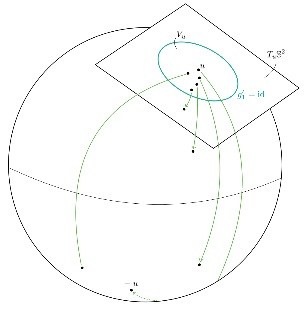
Figure 25. Illustration of the map $v\mapsto g^{\prime}_{1}(u,v)$ for $r=2$.

In fact, $g_{\tau}^{\prime}$ trivializes the sphere bundle globally: The isomorphism $g_{\tau}^{\prime}|_{\partial V}\colon\partial V\rightarrow Q_{t}\cap\partial\mathbb{B}$ is given by

$$(u,v) \mapsto e^{\mathrm{i}\theta}\Big{(}[u\cos\theta+v\sin\theta]\sqrt{\tfrac{1+\rho}{2}}+\mathrm{i}[v\cos\theta-u\sin\theta]\sqrt{\tfrac{1-\rho}{2}}\Big{)}\Big{|}_{\theta=\pi\tau}$$

$$=\left(\frac{u+\mathrm{i}v}{\sqrt{2}}\frac{R}{2}+\frac{u-\mathrm{i}v}{\sqrt{2}}\frac{t}{R}\right)_{R=\sqrt{1+\rho}+\sqrt{1-\rho}}$$

and therefore well-defined and smooth also over $t=0$, where it identifies $\partial V\cong Q_{0}\cap\partial\mathbb{B}$ as $(u,v)\mapsto(u+iv)/\sqrt{2}$. Hence, we can use $g_{1}^{\prime}$ to compute the localized variation. With the identification (A.5), the domain of

$$\operatorname{var}=(g_{1}^{\prime})_{*}-\operatorname{id}\colon\quad H_{r}(\overline{V},\partial V)\rightarrow H_{r}(V)$$

is $H_{r}(\overline{V},\partial V)\cong H_{0}(\mathbb{S}^{r})$ by the Thom isomorphism of the bundle $\mu\colon\overline{V}\rightarrow\mathbb{S}^{r}$, $(u,v)\mapsto u$. So for $r\geq 1$, $H_{r}(\overline{V},\partial V)\cong\mathbb{Z}$ is generated by the class of a fibre $\mu^{-1}(p)$. Over the point $p=(0,\ldots,0,1)\in\mathbb{S}^{r}$, this class $h=j_{*}[\overline{\mathbb{D}}]$ is represented by the $r$-dimensional disk $\overline{\mathbb{D}}=\{\lVert w\rVert\leq 1\}\subseteq\mathbb{R}^{r}$, embedded as

$$j\colon(\overline{\mathbb{D}},\partial\mathbb{D})\hookrightarrow(\overline{V},\partial V),\quad w\mapsto(p,(w,0))\in T_{p}\mathbb{S}^{r}.$$

Because the retraction $\mu$ induces an isomorphism $\mu_{*}\colon H_{r}(V)\cong H_{r}(\mathbb{S}^{r})\cong\mathbb{Z}$, we can compute the variation by pushing forward along $\mu$:

$$\mu_{*}(\operatorname{var}h)=\mu_{*}(g_{1}^{\prime})_{*}j_{*}[\overline{\mathbb{D}}]-\mu_{*}j_{*}[\overline{\mathbb{D}}].$$

Since $\mu j\colon\overline{\mathbb{D}}\rightarrow\mathbb{S}^{r}$ is the constant map $w\mapsto p$, the second term is zero in $H_{r}(\mathbb{S}^{r})\cong H_{r}(\mathbb{S}^{r},\{p\})$. The remaining term is the push-forward under

$$\mu g_{1}^{\prime}j\colon(\overline{\mathbb{D}},\partial\mathbb{D})\rightarrow(\mathbb{S}^{r},\{p\}),\quad w\mapsto\left(-\frac{w}{\lVert w\rVert}\sin(\pi\lVert w\rVert),\;-\cos(\pi\lVert w\rVert)\right).$$

This map is bijective on the interior $\mathbb{D}\cong\mathbb{S}^{r}\setminus\{p\}$ and realizes a homeomorphism $\overline{\mathbb{D}}/\partial\mathbb{D}\cong\mathbb{S}^{r}$. Therefore, we proved that

(A.6) $$\operatorname{var}\colon H_{r}(\overline{V},\partial V)\cong\mathbb{Z}\longrightarrow H_{r}(V)\cong\mathbb{Z},\quad h\mapsto\pm\nu$$

is an isomorphism. To fix the sign, we endow $\mathbb{D}\subset\mathbb{R}^{r}$ with the orientation $\mathrm{d}w_{1}\wedge\ldots\wedge\mathrm{d}w_{r}$. Under the differential of $u=\mu g_{1}^{\prime}j(w)$ at $w=0$, this becomes $(-1)^{r}\mathrm{d}u_{1}\wedge\ldots\wedge\mathrm{d}u_{r}$ at $T_{-p}\mathbb{S}^{r}$. In terms of the standard orientation on the vanishing sphere $\nu=[\mathbb{S}^{r}]$, this gives $\operatorname{var}h=-\nu$ in (A.6). The disk $j(\overline{\mathbb{D}})$ and the vanishing sphere $\mathbb{S}^{r}=\{v=0\}$ intersect in precisely one point, namely $(p,0)\in T_{p}\mathbb{S}^{r}$. According to appendix C, the intersection number

$$\langle{\nu}\,|\,{h}\rangle=\langle{[\mathbb{S}^{r}]}\,|\,{[j(\overline{\mathbb{D}})]}\rangle=\epsilon_{p}=\pm 1$$

is determined by comparing the orientation of the complex manifold $Q_{t}$ with the orientation of $T_{(p,0)}j(\overline{\mathbb{D}})\oplus T_{(p,0)}\mathbb{S}^{r}$. With our choices above, the latter is

($$\sharp \mathrm{d}v_{1}\wedge\ldots\wedge\mathrm{d}v_{r}\wedge(-1)^{r}\mathrm{d}u_{1}\wedge\ldots\wedge\mathrm{d}u_{r}.$$)

In terms of real and imaginary parts $x_{k}=\Re x_{k}+\mathrm{i}\Im x_{k}$, the orientation of $T_{p\sqrt{t}}Q_{t}$ induced from the complex structure is $\mathrm{d}\Re x_{1}\wedge\mathrm{d}\Im x_{1}\wedge\ldots\wedge\mathrm{d}\Re x_{r}\wedge\mathrm{d}\Im x_{r}$. In the parametrization (A.4), this is equal to

($$\natural \mathrm{d}u_{1}\wedge\mathrm{d}v_{1}\wedge\ldots\wedge\mathrm{d}u_{r}\wedge\mathrm{d}v_{r}\cdot\big{(}\sqrt{\lvert t\rvert(1-\lvert t\rvert)/2}\big{)}^{r}.$$)

The orientations ($\sharp$ ‣ A.2) and ($\natural$ ‣ A.2) differ by the sign $\epsilon_{p}=(-1)^{r}(-1)^{r(r+1)/2}$. We therefore arrive at the Picard-Lefschetz formula

$$\operatorname{var}h=-\nu=-(-1)^{r}(-1)^{r(r+1)/2}\langle{\nu}\,|\,{h}\rangle\nu=(-1)^{(r+1)(r+2)/2}\langle{\nu}\,|\,{h}\rangle\nu.$$

Remark A.10.

If $r=0$, then $V=\overline{V}=\mathbb{S}^{0}=\{p,-p\}$ consists of two points and $\partial V=\varnothing$. In this case, $\operatorname{var}\colon H_{0}(\mathbb{S}^{0})\rightarrow H_{0}(\mathbb{S}^{0})$ is a map from $\mathbb{Z}^{2}$ to $\mathbb{Z}^{2}$. The variations $\operatorname{var}[p]=-\nu$ and $\operatorname{var}[-p]=\nu=[p]-[-p]$ from 3.5 are indeed compatible with $\operatorname{var}h=(-1)^{1\cdot 2/2}\langle{\nu}\,|\,{h}\rangle\nu$.

Appendix B Partial boundaries and relative residues

B.1. Partial boundaries

Given any two topological subspaces $B,S\subseteq X$, we can consider the triple $B\subseteq B\cup S\subseteq X$ and its exact sequence

$$\cdots\rightarrow H_{\bullet}(X,B)\rightarrow H_{\bullet}(X,B\cup S)\xrightarrow{\partial}H_{\bullet-1}(B\cup S,B)\rightarrow H_{\bullet-1}(X,B)\rightarrow\cdots$$

The inclusion of pairs $(S,B\cap S)\rightarrow(B\cup S,B)$ induces a morphism

(B.1) $$H_{\bullet}(S,B\cap S)\longrightarrow H_{\bullet}(B\cup S,B).$$

Definition B.1.

A finite collection $(S_{i})_{i\in I}$ of smooth closed submanifolds $S_{i}\subset X$ is transverse if, for every subset $J\subseteq I$ and at every point $p\in S^{J}$ of the intersection $S^{J}=\bigcap_{i\in J}S_{i}$, the canonical projections $N_{p}S^{J}\longrightarrow N_{p}S_{i}$ assemble into isomorphisms $NS^{J}\cong\bigoplus_{i\in J}NS_{i}|_{S^{J}}$ of the normal bundles.

By the implicit function theorem, a transverse collection admits local coordinates $(x,(y_{i})_{i\in J})\colon U\longrightarrow\mathbb{R}^{d}\times\prod_{i\in J}\mathbb{R}^{r_{i}}$ near any point $p\in S^{J}$ such that $S_{i}\cap U=\{y_{i}=0\}$ for all $i\in J$, where $r_{i}=\operatorname{codim}S_{i}$ and $d=\dim S^{J}$. If each $S_{i}$ is a complex hypersurface ($r_{i}=2$) in a complex manifold, a transverse collection is also called simple normal crossings divisor.

Proposition B.2.

If $S=S_{1}$ and $B=\bigcup_{i>1}S_{i}$ form a transverse collection of smooth closed submanifolds $S_{i}\subset X$, then (B.1) is an isomorphism.

Proof.

Pick a tubular neighbourhood $u\colon N\hookrightarrow X$ of $S$, that is, a smooth embedding of the normal bundle $N=TX|_{S}/TS$ such that $u\iota=\operatorname{id}_{S}$ for the zero section $\iota\colon S\hookrightarrow N$. Let $U=u(N)$, then excise $B\setminus U$ to get

$$H_{\bullet}(B\cup S,B)\cong H_{\bullet}(S\cup(B\cap U),B\cap U).$$

Contraction $F_{\lambda}(v)=(1-\lambda)v$ of the fibres $N_{\pi(v)}$ shows that the projection $\pi=F_{1}\colon U\cong N\longrightarrow S$ is a deformation retract. Using the transversality assumption we may construct $u$ in such a way that $F_{\lambda}(U\cap B)\subseteq U\cap B$ for all $\lambda$, see [56, Lemma 4.3] or [27, Corollary 4.1]. Then $F_{\lambda}$ restricts to homotopies on $B\cap U$ and $S\cup(B\cap U)$, which proves that

$$\pi|_{B\cap U}\colon B\cap U\longrightarrow B\cap S\quad\text{and}\quad\pi|_{S\cup(B\cap U)}\colon S\cup(B\cap U)\longrightarrow S$$

are deformation retracts and induce isomorphisms $H_{\bullet}(B\cap U)\cong H_{\bullet}(B\cap S)$ and $H_{\bullet}(S\cup(B\cap U))\cong H_{\bullet}(S)$. To conclude, apply the five lemma to the long exact sequences of the pairs $(S\cup(B\cap U),B\cap U)$ and $(S,B\cap S)$. ∎

In this proof, we exploited the fact that one may choose tubular neighbourhoods $u_{i}\colon TX|_{S_{i}}/TS_{i}\hookrightarrow X$ for all $S_{i}$ in a mutually compatible way, such that $u_{i}^{-1}(S_{j})=TS_{j}|_{S_{i}\cap S_{j}}/TS_{i}|_{S_{i}\cap S_{j}}$. We will repeatedly use such compatible systems of tubes in this appendix. They are constructed in the references given in the proof above, see also [41, §7], and illustrated in fig. 26.

Definition B.3.

In the situation of B.2, the boundary in $S$ is the map $\partial_{S}\colon H_{\bullet}(X,B\cup S)\longrightarrow H_{\bullet-1}(S,B\cap S)$ obtained from the connecting morphism $\partial$ of the triple $B\subseteq B\cup S\subseteq X$ under the isomorphism (B.1):

Now the exact sequence of the triple $B\subseteq B\cup S\subseteq X$ takes the form

$$\cdots\rightarrow H_{\bullet}(X,B)\rightarrow H_{\bullet}(X,B\cup S)\xrightarrow{\partial_{S}}H_{\bullet-1}(S,B\cap S)\rightarrow H_{\bullet-1}(X,B)\rightarrow\cdots$$

B.2. Relative residues

If we replace $S$ by its complement $S^{\mathsf{c}}=X\setminus S$ and consider instead the triple $B\subseteq B\cup S^{\mathsf{c}}\subseteq X$, we get the sequence

$$\cdots\rightarrow H_{\bullet}(X,B)\rightarrow H_{\bullet}(X,B\cup S^{\mathsf{c}})\xrightarrow{\partial}H_{\bullet-1}(B\cup S^{\mathsf{c}},B)\rightarrow H_{\bullet-1}(X,B)\rightarrow\cdots$$

The inclusion of pairs $(S^{\mathsf{c}},B\setminus S)\rightarrow(B\cup S^{\mathsf{c}},B)$ induces a morphism

(B.2) $$H_{\bullet}(X\setminus S,B\setminus S)\longrightarrow H_{\bullet}(B\cup S^{\mathsf{c}},B).$$

Proposition B.4.

If $S=S_{1}$ and $B=\bigcup_{i\neq 1}S_{i}$ form a transverse collection of smooth closed submanifolds $S_{i}\subset X$, then (B.2) is an isomorphism.

Proof.

The zero section $S_{i}\hookrightarrow U_{i}$ of any tubular neighbourhood $NS_{i}\cong U_{i}\subseteq X$ induces an isomorphism $H_{\bullet}(S_{i})\cong H_{\bullet}(U_{i})$. Following [56, 27] we may assume the compatibility that every intersection $U^{J}=\bigcap_{i\in J}U_{i}$ is a tubular neighbourhood of $S^{J}$ (fig. 26), so that $H_{\bullet}(S^{J})\cong H_{\bullet}(U^{J})$.

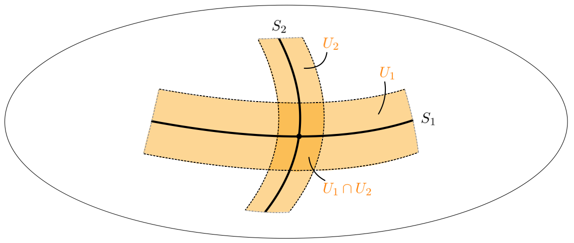
Figure 26. Tubular neighbourhoods of transverse submanifolds.

Then also the inclusion of $B$ into $U\mathrel{\mathop{:}}=\bigcup_{i\neq 1}U_{i}$ induces an isomorphism $H_{\bullet}(B)\cong H_{\bullet}(U),$ which follows from the Mayer-Vietoris sequence and the five lemma via induction over the number $\lvert I\rvert-1$ of components of $B$. Analogously, the inclusions $B\setminus S\hookrightarrow U\setminus S$ and $B\hookrightarrow B\cup(U\setminus S)$ induce isomorphisms

$$H_{\bullet}(B\setminus S)\cong H_{\bullet}(U\setminus S)\quad\text{and}\quad H_{\bullet}(B)\cong H_{\bullet}(B\cup(U\setminus S)),$$

because compatibility with $S_{1}$ ensures that for $1\notin J$, the projections $U^{J}\rightarrow S^{J}$ map $U^{J}\cap S$ to $S^{J}\cap S$ and restrict to deformation retracts $U^{J}\setminus S\rightarrow S^{J}\setminus S$ and $U^{J}\cap(B\cup S^{\mathsf{c}})\rightarrow S^{J}$. These thickenings of $B\setminus S$ and $B$ induce $H_{\bullet}(S^{\mathsf{c}},B\setminus S)\cong H_{\bullet}(S^{\mathsf{c}},U\setminus S)$ and $H_{\bullet}(B\cup S^{\mathsf{c}},B)\cong H_{\bullet}(B\cup S^{\mathsf{c}},B\cup(U\setminus S))$, and these isomorphisms identify (B.2) with the canonical map

$$H_{\bullet}(S^{\mathsf{c}},U\setminus S)\rightarrow H_{\bullet}(B\cup S^{\mathsf{c}},B\cup(U\setminus S)).$$

The interior of $B\cup(U\setminus S)$ in $B\cup S^{\mathsf{c}}$ contains $B\cap S$, thus the map above is an isomorphism by excision. ∎

To describe the group $H_{\bullet}(X,B\cup S^{\mathsf{c}})$, let $r=\operatorname{codim}S$ and consider a subbundle $\mu\colon V\rightarrow S$ of a tubular neighbourhood $NS\cong U\rightarrow S$ such that the fibres of $V\subset U$ are isomorphic to closed discs $\overline{\mathbb{B}}_{r}=\{x\in\mathbb{R}^{r}\colon\lVert x\rVert\leq 1\}$. Then we can excise the complement of $V$ to localize near $S$,

($$\ast H_{\bullet}(X,B\cup S^{\mathsf{c}})\cong H_{\bullet}(V,(B\cap V)\cup(V\setminus S)).$$)

For a transverse collection $S\cup B$, recall that we can choose $U\rightarrow S$ such that it preserves $B$. Then $\mu^{-1}(B\cap S)=V\cap B=V|_{B\cap S}$ is itself a disc bundle, namely the restriction of $V$ to $B\cap S$.

Definition B.5.

Suppose that the disc bundle $V\rightarrow S$ is oriented. Then the pullback bundle $\sigma^{\ast}V\cong\overline{\mathbb{B}}_{r}\times\Delta$ over a singular simplex $\sigma\colon\Delta\rightarrow S$ inherits an orientation, and hence descends to a well-defined map on homology:

(B.3) $$\mu_{S}^{\ast}\colon H_{\bullet}(S,B\cap S)\longrightarrow H_{\bullet+r}(X,B\cup S^{\mathsf{c}}).$$

Similarly, the pullback of the sphere bundle $\partial V\rightarrow S$ induces a map

(B.4) $$\delta_{S}\colon H_{\bullet}(S,B\cap S)\longrightarrow H_{\bullet+r-1}(S^{\mathsf{c}},B\setminus S)$$

called the Leray coboundary, such that $\partial(\mu_{S}^{\ast}[\sigma])=\delta_{S}[\sigma]+(-1)^{r}\mu_{S}^{\ast}(\partial[\sigma])$.

Proposition B.6.

If $S=S_{1}$ and $B=\bigcup_{i\neq 1}S_{i}$ form a transverse collection of smooth closed submanifolds $S_{i}\subset X$, and $S$ and $X$ are oriented, then the fibration-by-discs map (B.3) is an isomorphism.

Proof.

The orientations of $S$ and $X$ induce an orientation of the disc bundle $V$, and the complement $V^{\prime}\mathrel{\mathop{:}}=V\setminus S$ of the zero section deformation retracts onto the sphere bundle $\partial V$. So if $B=\varnothing$, then the excision ($\ast$ ‣ B.2) reduces the claim to the Thom isomorphism $H_{\bullet}(S)\rightarrow H_{\bullet+r}(V,V^{\prime})$.

For non-empty $B$, let $V_{B}\mathrel{\mathop{:}}=V\cap B=V|_{B\cap S}$ denote the restriction of $V$ to $B\cap S$ and consider the commutative diagram of the long exact sequences of the triple $V^{\prime}\subseteq V^{\prime}\cup V_{B}\subseteq V$ and the pair $B\cap S\subseteq S$:

The vertical maps are induced by the pullbacks of the disc bundle $V\rightarrow S$ and its restriction $V_{B}\rightarrow B\cap S$. The claim follows from the five lemma because $\nu$ is an isomorphism. Indeed, by construction $\nu$ factors into

$$H_{\bullet}(B\cap S)\rightarrow H_{\bullet+r}(V_{B},V_{B}^{\prime})\rightarrow H_{\bullet+r}(V_{B}\cup V^{\prime},V^{\prime})$$

where $V_{B}^{\prime}\mathrel{\mathop{:}}=V_{B}\setminus S=V_{B}\cap V^{\prime}$ and the first map is the Thom isomorphism for the bundle $V_{B}$. The second map is an isomorphism because $V^{\prime}$ and $V_{B}$ constitute an excisive couple, by the thickening principle from the proof of B.4: replace $V_{B}$ by an open neighbourhood $V\cap U\cap(V^{\prime}\cup V_{B})$ inside $V^{\prime}\cup V_{B}$ with the same homology as $V_{B}$, obtained from a union $U$ of compatible tubular neighbourhoods of the components of $B$. ∎

Combining this result with B.4, we can write the long exact sequence of the triple $B\subseteq B\cup S^{\mathsf{c}}\subseteq X$ for a transverse collection of oriented smooth closed submanifolds as the relative residue sequence

$$\cdots\rightarrow H_{\bullet}(X,B)\xrightarrow{\varpi_{S}}H_{\bullet-r}(S,B\cap S)\xrightarrow{\delta_{S}}H_{\bullet-1}(X\setminus S,B\setminus S)\rightarrow H_{\bullet-1}(X,B)\rightarrow\cdots$$

where the map $\varpi_{S}$ can be interpreted as “transverse intersection with $S$”. It is defined by the commutative diagram

B.3. Functoriality and commutativity

Let $r_{i}$ denote the codimension of a submanifold $S_{i}\subset X$ in a transverse family. Then the maps $(\partial_{S_{i}},\delta_{S_{i}},\varpi_{S_{i}})$ have homological degrees $(-1,r_{i}-1,-r_{i})$, and for $i\neq j$ they are graded commutative with the same degrees:

(B.5) $$\partial_{S_{i}}\partial_{S_{j}} =-\partial_{S_{j}}\partial_{S_{i}} \delta_{S_{i}}\delta_{S_{j}} =(-1)^{(r_{i}-1)(r_{j}-1)}\delta_{S_{j}}\delta_{S_{i}}$$

$$\partial_{S_{i}}\delta_{S_{j}} =(-1)^{r_{j}-1}\delta_{S_{j}}\partial_{S_{i}} \delta_{S_{i}}\varpi_{S_{j}} =(-1)^{(r_{i}-1)r_{j}}\varpi_{S_{j}}\delta_{S_{i}}$$

$$\partial_{S_{i}}\varpi_{S_{j}} =(-1)^{r_{j}}\varpi_{S_{j}}\partial_{S_{i}} \varpi_{S_{i}}\varpi_{S_{j}} =(-1)^{r_{i}r_{j}}\varpi_{S_{j}}\varpi_{S_{i}}$$

The first identity amounts to $\partial^{2}=0$ and the other signs compare the induced orientations on the disc and sphere bundles, see also [39, Proposition 39]. Furthermore, suppose that a smooth map $F\colon X\longrightarrow X^{\prime}$ restricts to submersions $S_{i}\longrightarrow S_{i}^{\prime}\mathrel{\mathop{:}}=F(S_{i})$ onto a transverse family $(S_{i}^{\prime})_{i\in I}$ in $X^{\prime}$. Then the maps commute with pushforward:

(B.6) $$F_{\ast}\partial_{S_{i}}=\partial_{S_{i}^{\prime}}F_{\ast},\quad F_{\ast}\delta_{S_{i}}=\delta_{S_{i}^{\prime}}F_{\ast},\quad F_{\ast}\varpi_{S_{i}}=\varpi_{S_{i}^{\prime}}F_{\ast}.$$

Appendix C Relative intersection numbers

Consider a smooth compact oriented manifold $\overline{M}$ of dimension $n$, with boundary $\partial M=\overline{M}\setminus M$ (possibly empty) and interior $M$. The cap product with the fundamental class $[M]\in H_{n}(\overline{M},\partial M)$ defines a homomorphism

$$\Psi\colon H^{d}(M)\longrightarrow H_{n-d}(\overline{M},\partial M),\quad\alpha\mapsto[M]\frown\alpha$$

from singular cohomology, to homology in complementary degree. Poincaré-Lefschetz duality states that this is an isomorphism [62, Theorem 6.25, p. 171]. The duality $H_{d}(M)\times H^{d}(M)\rightarrow\mathbb{Z}$ can thus be viewed as a bilinear map

$$\langle{\cdot}\,|\,{\cdot}\rangle\colon H_{d}(M)\times H_{n-d}(\overline{M},\partial M)\longrightarrow\mathbb{Z},\quad\langle{x}\,|\,{y}\rangle=(\Psi^{-1}(y))(x).$$

These intersection numbers can be computed as follows: If $x=[Q]$ and $y=[R]$ are fundamental classes of compact oriented submanifolds $Q$ and $R$ ($\partial Q=\varnothing$ and $\partial R\subseteq\partial M$) that intersect transversally, then $Q\cap R\subseteq M$ is also a compact oriented submanifold—in fact, it is a finite set of points. Then

$$\langle{[Q]}\,|\,{[R]}\rangle=\sum_{p\in Q\cap R}\epsilon_{p},$$

with signs $\epsilon_{p}=\pm 1$ determined by the orientations. We follow the convention in [51], namely that $\epsilon=+1$ precisely when the orientation of $M$ at $p$ agrees with the orientation of first $R$, then $Q$, under the identification

($$\flat T_{p}M=T_{p}R\oplus T_{p}Q.$$)

When $x$ and $y$ are not presented by transverse submanifolds, one can perturb the singular simplices slightly to obtain homologous chains with transverse simplices, and apply the same recipe; cf. [54, §73] and [17, §VII.4].

If $\partial M=\varnothing$, we can swap $x$ and $y$. Then from ($\flat$ ‣ C) it follows that

(C.1) $$\langle{x}\,|\,{y}\rangle=(-1)^{d(n-d)}\cdot\langle{y}\,|\,{x}\rangle.$$

Remark C.1.

The sign convention is more intuitive in terms of the normal bundles $NR=TM|_{R}/TR$ and $NQ=TM|_{Q}/TQ$. From ($\flat$ ‣ C) we see $N_{p}R\cong T_{p}Q$ and $N_{p}Q\cong T_{p}R$, hence $\epsilon_{p}=+1$ if the orientations on the normal bundles agree, under the canonical isomorphism

($$\natural N_{p}(Q\cap R)\cong N_{p}Q\oplus N_{p}R$$)

with the normal bundles of first $Q$, then $R$ (the same order as in “$\langle{[Q]}\,|\,{[R]}\rangle$”). Note that ($\natural$ ‣ C.1) holds for transverse intersections of arbitrary dimensions $i=\dim Q$ and $j=\dim R$, whereas ($\flat$ ‣ C) only applies for $i+j=n$. The orientation of $Q\cap R$ induced by ($\natural$ ‣ C.1) generalizes the intersection numbers to the intersection product $[Q]\bullet[R]=[Q\cap R]\in H_{i+j-n}(M)$, see [17, §VIII.13].

C.1. Transverse arrangements

Inside a smooth compact oriented manifold $\overline{M}$ as above, consider a transverse arrangement $D=A\cup B=\bigcup_{i}D_{i}$ of smooth oriented closed submanifolds $D_{i}$. If $\partial M\neq\varnothing$, we also require that $D$ is transverse to $\partial M$. Then the intersection numbers define a bilinear pairing

(C.2) $$\langle{\cdot}\,|\,{\cdot}\rangle\colon H_{d}(M\setminus B,A)\times H_{n-d}(\overline{M}\setminus A,\partial M\cup B)\longrightarrow\mathbb{Z}.$$

For transverse submanifolds $Q\subseteq M\setminus B$, $R\subseteq\overline{M}\setminus A$ with $\partial Q\subseteq A$ and $\partial R\subseteq B\cup\partial M$, their intersection is a finite set of points inside $M\setminus D$, and $\langle{[Q]}\,|\,{[R]}\rangle$ can be computed as above. In general, the intersection pairing is constructed in [17, §VII.4]. In fact, we can define (C.2) as the composition of:

• the Künneth morphism for the product $Y=(M\setminus B)\times(\overline{M}\setminus A)$, relative to $D^{\prime}=A\times(\overline{M}\setminus A)\cup(M\setminus B)\times(\partial M\cup B)$:

  $$H_{d}(M\setminus B,A)\otimes H_{n-d}(\overline{M}\setminus A,\partial M\cup B)\longrightarrow H_{n}(Y,D^{\prime})$$

• intersection with the diagonal $\Delta=\{(p,p)\colon p\in M\}\cap Y\cong M\setminus D$:

  $$H_{n}(Y,D^{\prime})\xrightarrow{\varpi_{\Delta}}H_{0}(\Delta,D^{\prime}\cap\Delta)\cong H_{0}(M\setminus D)\cong\mathbb{Z}.$$

Here note that $D^{\prime}\cap\Delta=\varnothing$, and the map $\varpi_{\Delta}$ from the Gysin/residue sequence is constructed in appendix B: work relative to $D^{\prime}\cup(Y\setminus\Delta)$, excise all but a tubular neighbourhood of $\Delta$, and apply the Thom isomorphism.

C.2. Duality

Consider a submanifold $S\in\mathfrak{B}$ of real codimension $r$. Let $B^{\prime}\subseteq B$ denote the union of the remaining $B_{i}\neq S$. Then the intersection pairings on $M$ and $S$ are compatible in the following sense: If $x\in H_{d}(S\setminus B^{\prime},A)$ and $y\in H_{n-d-r+1}(\overline{M}\setminus A,\partial M\cup B)$, then

(C.3) $$\langle{\delta_{S}\,x}\,|\,{y}\rangle=(-1)^{1+(r-1)(n-d)}\cdot\langle{x}\,|\,{\partial_{S}\,y}\rangle.$$

This is a simple generalization of [51, §III.2.3]. Equivalently, swapping the roles of $x$ and $y$ as in (C.1) when $S\in\mathfrak{A}$, we have for $x\in H_{d}(M\setminus B,A)$ and $y\in H_{n-d-r+1}(\overline{S}\setminus A^{\prime},\partial S\cup B)$ the identity

$$\langle{\partial_{S}\,x}\,|\,{y}\rangle=(-1)^{1+d+n}\cdot\langle{x}\,|\,{\delta_{S}\,y}\rangle.$$

Hence in the case of a complex hypersurface $S\subset M$ ($r=2$ and $n$ even), we obtain for homology classes $x$ of degree $d$ that

(C.4) $$\langle{\delta_{S}\,x}\,|\,{y}\rangle =(-1)^{1+d}\cdot\langle{x}\,|\,{\partial_{S}\,y}\rangle\quad\text{and}$$

$$\langle{\partial_{S}\,x}\,|\,{y}\rangle =(-1)^{1+d}\cdot\langle{x}\,|\,{\delta_{S}\,y}\rangle.$$

For an Abelian group $G$, let $G^{\vee}=\operatorname{Hom}(G,\mathbb{Z})$ denote its dual. The pairing (C.2) defines a map $H_{d}(M\setminus B,A)\rightarrow H_{n-d}(\overline{M}\setminus A,\partial M\cup B)^{\vee}$. Extend to rational coefficients, then the codomain is canonically isomorphic to singular cohomology, by the universal coefficient theorem. This defines a linear map

(C.5) $$H_{d}(M\setminus B,A;\mathbb{Q})\longrightarrow H^{n-d}(\overline{M}\setminus A,\partial M\cup B;\mathbb{Q}).$$

Theorem C.2.

The intersection pairing (C.2) is perfect modulo torsion. In other words, (C.5) is an isomorphism.

Proof.

When $A=B=\varnothing$, this is just a restatement of the Poincaré-Lefschetz theorem. With this as a base case, the proof follows by induction over the number of elements of the arrangement $\mathfrak{D}=\mathfrak{A}\sqcup\mathfrak{B}$:

Consider an element $S\in\mathfrak{B}$, so that $B=S\cup B^{\prime}$ where $B^{\prime}$ is the union of all $B_{i}$ in $\mathfrak{B}\setminus\{S\}$. The residue and boundary sequences from appendix B fit into the diagram

built out of the residue sequence in the left column, the dual of the boundary sequence in the right column, and the horizontal maps induced by the intersection pairings. We can add signs such that this diagram commutes: one of the squares is (C.3), and similarly one checks that the other squares also commute up to sign. We may assume that $\alpha\otimes\mathbb{Q}$ and $\beta\otimes\mathbb{Q}$ are isomorphisms, because they arise from intersection pairings of smaller arrangements $\mathfrak{D}\setminus\{S\}$. The induction step then follows from the five-lemma.

Analogously, we can add an element $S\in\mathfrak{A}$, by considering the diagram built from the boundary sequence (left column) and the dual of the residue sequence (right column). ∎

C.3. de Rham cohomology

Under the identification (C.5), the intersection pairing can be viewed as a perfect pairing in singular cohomology,

$$H^{d}(M\setminus B,A;\mathbb{Q})\times H^{n-d}(\overline{M}\setminus A,\partial M\cup B;\mathbb{Q})\longrightarrow\mathbb{Q}.$$

Consider now the special case when $M$ is a compact complex manifold without boundary, and $D\subset M$ is a transverse union of smooth complex hypersurfaces. Let $H_{\mathsf{dR}}^{\bullet}$ denote the cohomology of smooth complex differential forms. By the de Rham theorem $H_{\mathsf{dR}}^{\bullet}\cong H^{\bullet}\otimes\mathbb{C}$, we obtain a perfect pairing

(C.6) $$H_{\mathsf{dR}}^{d}(M\setminus B,A)\times H_{\mathsf{dR}}^{n-d}(M\setminus A,B)\longrightarrow\mathbb{C}.$$

This incarnation of C.2 is derived in [11, §3] from Verdier duality. Furthermore, by [11, Proposition 3.10] the pairing (C.6) equals the integral

$$([\nu],[\omega])\longmapsto\int_{M}\nu\wedge\omega.$$

Here the representative forms $\nu$ ($\omega$) have to be chosen such that they have at most simple poles on $B$ ($A$). This is always possible [39, pp. 121–122], and ensures that the integral converges. When $M$ and $D$ are algebraic over $\mathbb{Q}$, then the pairing (C.6) also respects the $\mathbb{Q}$-mixed Hodge structures on algebraic de Rham cohomology [11].

Appendix D Fundamental group and small loops

Consider a closed analytic subvariety $L\subsetneq T$ of a connected complex manifold $T$. Let $\mathfrak{L}$ denote the subset of irreducible components of $L$ which have complex codimension one. Their union forms a subset $L^{\prime}=\bigcup_{\ell\in\mathfrak{L}}\ell\subseteq L$.

Proposition D.1.

Fix a point $t\in T\setminus L$ and take all fundamental groups in the sequel relative to $t$ as the base point. Then:

1. The inclusion $T\setminus L\hookrightarrow T\setminus L^{\prime}$ induces an isomorphism

   $$\pi_{1}(T\setminus L)\xrightarrow{\;\cong\;}\pi_{1}(T\setminus L^{\prime}).$$

2. The inclusion $T\setminus L\hookrightarrow T$ induces a surjection

   $$\iota\colon\pi_{1}(T\setminus L)\relbar\joinrel\twoheadrightarrow\pi_{1}(T).\qquad\quad$$

3. The kernel of $\iota$ is generated by simple loops (3.1).

Corollary D.2.

The fundamental group of $T\setminus L$ depends only on the codimension one part $L^{\prime}$ of $L$. When $T$ is simply connected, then $\pi_{1}(T\setminus L)$ is generated by simple loops.

D.1 follows from the existence of stratifications by smooth subvarieties (section 2) and transverse deformations. A smooth map $f\colon X\rightarrow Y$ of manifolds is called transverse to a closed submanifold $D\subset Y$, if at every point $x\in X$ with $f(x)\in D$, the tangent space of $Y$ is spanned by the tangent space of $D$ and the image of the differential of $f$:

$$T_{f(x)}Y=T_{f(x)}D+\mathrm{d}f_{x}\left(T_{x}X\right).$$

Under this condition, $f^{-1}(D)$ is a closed submanifold of $X$, with codimension $\dim Y-\dim D$. In particular, if $\dim D+\dim X<\dim Y$, then transversality implies that the image of $f$ does not intersect $D$, that is $f(X)\subseteq Y\setminus D$.

Theorem D.3 (Transversality theorem [33, §IV.Corollary (2.5)]).

Given a smooth closed submanifold $D\subset Y$ and a smooth map $f\colon X\rightarrow Y$, there exists a smooth map that is homotopic to $f$ and transverse to $D$.

Corollary D.4 ([22, Théorème 2.3]).

For a closed smooth submanifold $D\subset Y$ of real codimension $r\geq 2$, the morphism $\pi_{1}(Y\setminus D)\rightarrow\pi_{1}(Y)$, induced by the inclusion $Y\setminus D\hookrightarrow Y$, is surjective. Whenever $r\geq 3$, it is also injective.

Proof.

Every loop $\gamma\colon[0,1]\rightarrow Y$ is homotopic to a loop $\gamma^{\prime}$ that is transverse to $D$. Because $\dim D+\dim\,[0,1]=\dim Y-r+1$ and $r\geq 2$, $\gamma^{\prime}$ does not intersect $D$, proving surjectivity. For injectivity, suppose $[\gamma]\in\pi_{1}(Y\setminus D)$ is in the kernel, i.e. there is a contracting homotopy $F\colon[0,1]^{2}\rightarrow Y$ of $\gamma$ in $Y$. Choose $F$ transverse to $D$. Then since $\dim([0,1]^{2})=2$ and $r\geq 3$, the homotopy does not intersect $D$. Thus $\gamma$ is contractible already in $Y\setminus D$. ∎

Proof of D.1.

The subvariety $L\setminus L^{\prime}$ of $Y=T\setminus L^{\prime}$ has complex codimension at least two (definition of $L^{\prime}$). Consider a stratification $L\setminus L^{\prime}=C_{n-2}\supseteq\cdots\supseteq C_{0}$ by closed analytic subvarieties $C_{k}$, so that each difference $D_{k}=C_{k}\setminus C_{k-1}$ is a smooth closed complex submanifold of $Y\setminus C_{k-1}$, with real codimension $2n-2k\geq 4$. By D.4, inclusions induce isomorphisms

($$\ast \iota_{k}\colon\pi_{1}(Y\setminus C_{k})\longrightarrow\pi_{1}(Y\setminus C_{k-1})$$)

for each $k\leq n-2$. Their composition $\iota_{0}\cdots\iota_{n-2}$ yields the isomorphism (1) between the fundamental groups of $Y\setminus C_{n-2}=T\setminus L$ and $Y=T\setminus L^{\prime}$.

The claim (2) is proved analogously, by considering a stratification of $L=C_{n-1}\supseteq\cdots\supseteq C_{0}$ inside $Y=T$. As above, the maps ($\ast$ ‣ D) are isomorphisms for $k\leq n-2$. At $k=n-1$, we still have surjectivity (real codimension two).

Given the isomorphisms $\pi_{1}(T\setminus C_{n-2})\cong\pi_{1}(T\setminus C_{n-3})\cong\cdots\cong\pi_{1}(T)$, we set $Y=T\setminus C_{n-2}$ and identify the map $\iota$ in claim (3) with the morphism

$$\pi_{1}(T\setminus L)=\pi_{1}(Y\setminus D)\longrightarrow\pi_{1}(Y)\cong\pi_{1}(T)$$

induced by the inclusion of the complement $T\setminus L=Y\setminus D$ of the smooth submanifold $D=L\setminus C_{n-2}\subset Y$, which has real codimension two. We apply the proof of [51, Proposition §V.1.3]: For $[\gamma]\in\pi_{1}(Y\setminus D,t)$ in the kernel of $\iota$, there is a homotopy $F\colon\square\rightarrow Y$ on the square $\square=[0,1]^{2}$ with $F(\tau,1)=F(0,\tau)=F(1,\tau)=t$ constant and $\gamma(\tau)=F(\tau,0)$. Choose $F$ transverse to $D$, so $P=\{p_{1},\ldots,p_{k}\}=F^{-1}(D)$ is a submanifold—with dimension zero (a finite set of points). In the group $\pi_{1}(\square\setminus P)$, the boundary of the square is a product of simple loops $\gamma_{i}$ (fig. 27), hence, applying $F$,

$$[\gamma]=\eta_{1}\star\cdots\star\eta_{k}$$

is a product of simple loops $\eta_{i}=[F\circ\gamma_{i}]\in\pi_{1}(Y\setminus D,t)$ around $t_{i}=F(p_{i})\in D$. Consider a holomorphic chart $(z_{1},\ldots,z_{d})$ of $Y$, centered at $t_{i}$, with locally $D=\{z_{1}=0\}$. By transversality of $F$, the map $q\mapsto z_{1}(F(q))$ is a local diffeomorphism and embeds a sufficiently small disk $\mathbb{D}=\{q\in\square\colon\lVert q-p\rVert<\epsilon\}$. As $\gamma_{i}$ is conjugate to the circle $\partial\mathbb{D}$, the loop $\eta_{i}$ is conjugate to the closed curve $F(\partial\mathbb{D})=\partial(F(\mathbb{D}))$. The latter winds once around $t_{i}=\{z=0\}=F(\mathbb{D})\cap L$, and it is homotopic to $\{\lvert z_{1}\rvert=\epsilon\}\times\{z_{2}=\cdots=z_{d}=0\}\subset T\setminus L$. Thus indeed, $\eta_{i}$ (or its inverse, depending on the orientation) represents the class of a simple loop in the sense of 3.1. ∎

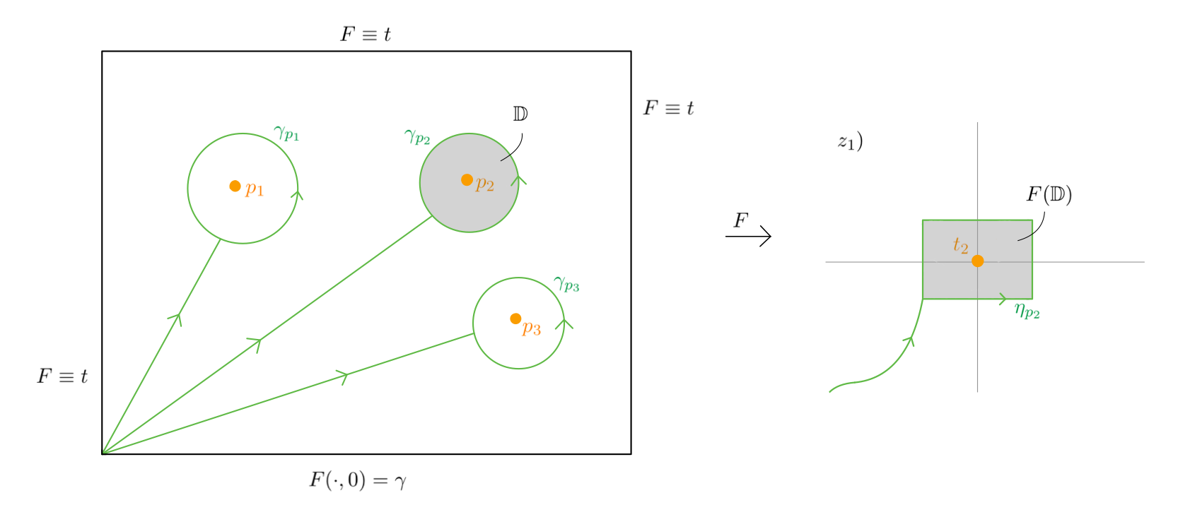
Figure 27. Decomposition of a homotopy into simple loops.

Remark D.5.

Instead of transversality, one can prove D.1 and D.4 also with the Seifert–van Kampen theorem. Consider the open cover $Y=Y\setminus D\cup N$ obtained from a tubular neighbourhood $N\supset D$. By induction over the connected components, we may assume that $D$ is connected. Then we can write the amalgamated product as

(D.1) $$\pi_{1}(Y)\cong\pi_{1}(Y\setminus D)*_{\pi_{1}(S)}\pi_{1}(D),$$

exploiting the homotopy equivalences $N\simeq D$ and $N\setminus D\simeq S$, where $S\subset N$ denotes a sphere bundle with fibre $\mathbb{S}^{r-1}$. Since the fibre is connected ($r\geq 2$), the long exact homotopy sequence for the bundle $S$ ends in

$$\cdots\rightarrow\pi_{1}(\mathbb{S}^{r-1})\rightarrow\pi_{1}(S)\xrightarrow{\alpha}\pi_{1}(D)\rightarrow 0.$$

The surjectivity of $\alpha$ renders the factor $\pi_{1}(D)$ in (D.1) superfluous, proving that $\iota\colon\pi_{1}(Y\setminus D)\rightarrow\pi_{1}(Y)$ surjects. In consequence, the amalgamated product degenerates to a quotient

$$\pi_{1}(Y)\cong\pi_{1}(Y\setminus D)/\langle G\rangle,$$

where $\ker\iota=\langle G\rangle$ denotes the normal closure of the leftover relations, where $G$ denotes the image in $\pi_{1}(Y\setminus D)$ of the kernel of $\alpha$. For $r\geq 3$, the groups $\pi_{1}(\mathbb{S}^{r-1})=0$ and thus $\ker\alpha$ are trivial, so that $\iota$ is injective.

Finally, if $r=2$, $\pi_{1}(\mathbb{S}^{1})\cong\mathbb{Z}$ shows that $G$ is generated by a single small loop $\gamma$ around $D$. Thus the entire kernel $\langle G\rangle$ of $\iota$ is generated by the conjugates of $\gamma$. This generation by a single element and its conjugates is explained also in [32, Lemme 1.2].

Remark D.6.

Any two simple loops $\gamma$, $\gamma^{\prime}$ around the same component $\ell\in\mathfrak{L}$ are conjugate. Indeed, by definition,

$$\gamma=\eta^{-1}\star\partial\mathbb{D}\star\eta\quad\text{and}\quad\gamma^{\prime}={\eta^{\prime}}^{-1}\star\partial\mathbb{D}^{\prime}\star\eta^{\prime}$$

are conjugate to the the boundary circles $\partial\mathbb{D}\cong\mathbb{S}^{1}$ of small holomorphic discs $\mathbb{D}$, $\mathbb{D}^{\prime}$ embedded transverse to the smooth part $S=\ell\setminus C_{n-2}$. We can shrink them to fit into a tubular neighbourhood $N\supset S$, so that $\partial\mathbb{D}\simeq\pi^{-1}(t_{c})$ and $\partial\mathbb{D}^{\prime}\simeq\pi^{-1}(t_{c}^{\prime})$ are homotopic to fibres of the corresponding circle bundle $\pi\colon\partial N\rightarrow S$. Since $S$ is connected, there is a path $\rho\colon[0,1]\rightarrow S$ that connects $t_{c}$ and $t_{c}^{\prime}$. The pullback $\rho^{-1}\pi\cong[0,1]\times\mathbb{S}^{1}$ is a cylinder and supplies a homotopy $\partial\mathbb{D}\simeq\partial\mathbb{D}^{\prime}$; as paths with basepoints, these circles are conjugate.

The closure $S\mapsto\overline{S}$ gives a bijection between the connected components $S\subseteq D=L\setminus C_{n-2}$ (strata of complex codimension one), and the Landau singularities $\mathfrak{L}$ (the irreducible components of $L^{\prime}$).

For every $\ell\in\mathfrak{L}$, choose an arbitrary simple loop $\gamma_{\ell}$ around $\ell$. Then by the previous remark, their conjugates provide the set

$$H=\{\eta^{-1}\star\gamma_{\ell}\star\eta\colon\ell\in\mathfrak{L}\ \text{and}\ \eta\in\pi_{1}(T\setminus L)\}.$$

of all simple loops. Part (3) of D.1 states that the kernel of $\iota$ is the subgroup generated by $H$.

Remark D.7.

The subgroup generated by the simple loops $H^{\prime}=\{\gamma_{\ell}\colon\ell\in\mathfrak{L}\}$ alone, without including conjugates, can be strictly smaller. For example, [52, Theorem 2] constructs, among several others, a smooth embedding

$$L=\ell\sqcup\ell^{\prime}\quad\hookrightarrow\quad Y=\mathbb{S}^{6}$$

of two disjoint spheres $\ell\cong\ell^{\prime}\cong\mathbb{S}^{4}$ with the following property: For every choice of simple loops $\gamma_{\ell}$ and $\gamma_{\ell^{\prime}}$, the group generated by $H^{\prime}=\{\gamma_{\ell},\gamma_{\ell^{\prime}}\}$ is strictly smaller than the kernel of $\pi_{1}(Y\setminus L)\rightarrow\pi_{1}(Y)$.

Thus the monodromy representation is not necessarily completely determined by the variation along only one simple loop per Landau component.

References

- [1] K. Aomoto, Analytic structure of Schläfli function, Nagoya Math. J. 68 (1977) pp. 1–16.
- [2] K. Aomoto, Addition theorem of Abel type for hyper-logarithms, Nagoya Mathematical Journal 88 (1982) pp. 55–71.
- [3] N. Arkani-Hamed, A. Hillman and S. Mizera, Feynman polytopes and the tropical geometry of UV and IR divergences, Phys. Rev. D 105 (June, 2022) p. 125013, arXiv:2202.12296 [hep-th].
- [4] N. Arkani-Hamed and E. Y. Yuan, “One-loop integrals from spherical projections of planes and quadrics.” preprint, Dec., 2017, arXiv:1712.09991 [hep-th].
- [5] E. Arnold, S. Gusein-Zade and A. N. Varchenko, Singularities of Differentiable Maps, Volume 2. Modern Birkhäuser Classics. Birkhäuser, Boston, 1st ed., 2012.
- [6] S. Bloch, H. Esnault and D. Kreimer, On motives associated to graph polynomials, Commun. Math. Phys. 267 (2006), no. 1 pp. 181–225, arXiv:math/0510011.
- [7] C. Bogner and S. Weinzierl, Feynman graph polynomials, Int. J. Mod. Phys. A 25 (2010) pp. 2585–2618, arXiv:1002.3458 [hep-ph].
- [8] J. L. Bourjaily, H. Hannesdottir, A. J. McLeod, M. D. Schwartz and C. Vergu, Sequential discontinuities of Feynman integrals and the monodromy group, JHEP 2021 (Jan., 2021) p. 205, arXiv:2007.13747 [hep-th].
- [9] J. B. Boyling, Construction of vanishing cycles for integrals over hyperspheres, Journal of Mathematical Physics 7 (Oct., 1966) pp. 1749–1763.
- [10] J. B. Boyling, A homological approach to parametric Feynman integrals, Il Nuovo Cimento A 53 (1968), no. 2 pp. 351–375.
- [11] F. Brown and C. Dupont, Single-valued integration and double copy, J. Reine Angew. Math. 2021 (2021), no. 775 pp. 145–196, arXiv:1810.07682 [math.NT].
- [12] F. C. S. Brown, “On the periods of some Feynman integrals.” preprint, Oct., 2009, arXiv:0910.0114 [math.AG].
- [13] F. C. S. Brown, Feynman amplitudes, coaction principle, and cosmic Galois group, Commun. Number Theory Phys. 11 (2017), no. 3 pp. 453–556, arXiv:1512.06409 [math-ph]. recorded lectures: 1, 2, 3, 4) (IHÉS 2015).
- [14] F. C. S. Brown and D. Kreimer, Angles, scales and parametric renormalization, Lett. Math. Phys. 103 (2013), no. 9 pp. 933–1007, arXiv:1112.1180 [hep-th].
- [15] S. Caron-Huot, L. J. Dixon, F. Dulat, M. von Hippel, A. J. McLeod and G. Papathanasiou, The cosmic Galois group and extended Steinmann relations for planar SYM amplitudes, Journal of High Energy Physics 2019 (Sept., 2019) p. 61, arXiv:1906.07116 [hep-th].
- [16] J. L. Cisneros-Molina and J. Seade, Milnor’s fibration theorem for real and complex singularities, in Handbook of Geometry and Topology of Singularities II (J. L. Cisneros-Molina, D. T. Lê and J. Seade, eds.), pp. 309–359. Springer, 2021.
- [17] A. Dold, Lectures on algebraic topology, vol. 200. Springer, 1972.
- [18] J. Drummond, J. Foster and O. Gürdoğan, Cluster Adjacency Properties of Scattering Amplitudes in Supersymmetric Yang-Mills Theory, Phys. Rev. Lett. 120 (Apr., 2018) p. 161601, arXiv:1710.10953 [hep-th].
- [19] I. Fáry, Self-intersection of a sphere on a complex quadric, Pac. J. Math. 11 (1961), no. 4 pp. 1251–1255.
- [20] P. Federbush, Calculation of some homology groups relevant to sixth-order Feynman diagrams, Journal of Mathematical Physics 6 (1965), no. 6 pp. 941–954.
- [21] D. Fotiadi, M. Froissart, J. Lascoux and F. Pham, Applications of an isotopy theorem, Topology 4 (1965), no. 2 pp. 159–191.
- [22] C. Godbillon, Éléments de topologie algébrique. Collection Méthodes. Hermann, nouv. tirage ed., 1998.
- [23] V. A. Golubeva, Investigation of Feynman integrals by homological methods, Theoretical and Mathematical Physics 3 (June, 1970) pp. 604–615.
- [24] M. Goresky and R. MacPherson, Stratified Morse Theory, vol. 14 (Folge 3) of Ergebnisse der Mathematik und ihrer Grenzgebiete. Springer, 1988.
- [25] H. Grauert and R. Remmert, Coherent Analytic Sheaves, vol. 265 of Grundlehren der mathematischen Wissenschaften. Spinger-Verlag, Berlin, 1984.
- [26] P. A. Griffiths, Periods of integrals on algebraic manifolds: Summary of main results and discussion of open problems, Bull. Amer. Math. Soc. 76 (1970) pp. 228–296.
- [27] R. Guadagni, “Symplectic neighborhood of crossing divisors.” preprint, Nov., 2016, arXiv:1611.02363 [math.SG].
- [28] H. Hamm, Lokale topologische Eigenschaften komplexer Räume, Math. Ann. 191 (1971), no. 3 pp. 235–252.
- [29] H. S. Hannesdottir, A. J. McLeod, M. D. Schwartz and C. Vergu, “Constraints on sequential discontinuities from the geometry of on-shell spaces.” preprint, Nov., 2022, arXiv:2211.07633 [hep-th].
- [30] M. Hirsch, Differential Topology, vol. 33 of Graduate Text in Mathematics. Springer, 1st ed., 1976.
- [31] R. C. Hwa and V. L. Teplitz, Homology and Feynman integrals. The mathematical physics monograph series. W. A. Benjamin, Inc., New York, 1966.
- [32] M. Kervaire, Les nœuds de dimensions supérieures, Bull. Soc. Math. Fr. 93 (1965) pp. 225–271.
- [33] A. A. Kosinski, Differential manifolds, vol. 138 of Pure and applied mathematics. Academic Press, Boston, 1993.
- [34] K. Lamotke, Die Homologie isolierter Singularitäten, Math. Z. 143 (1975) pp. 27–44.
- [35] K. Lamotke, The topology of complex projective varieties after S. Lefschetz, Topology 20 (1981), no. 1 pp. 15–51.
- [36] P. V. Landshoff, D. I. Olive and J. C. Polkinghorne, The hierarchical principle in perturbation theory, Il Nuovo Cimento A 43 (1966), no. 2 pp. 444–453.
- [37] P. V. Landshoff, J. C. Polkinghorne and J. C. Taylor, Proof of the Mandelstam representation in perturbation theory, Il Nuovo Cimento 19 (1961).
- [38] M. Lassalle, Analyticity properties implied by the many-particle structure of the -point function in general quantum field theory. 1. convolution of point functions associated with a graph, Commun. Math. Phys. 36 (1974), no. 3 pp. 185–226.
- [39] J. Leray, Le calcul différentiel et intégral sur une variété analytique complexe. (Problème de Cauchy. III), Bull. Soc. Math. France 87 (1959) pp. 81–180.
- [40] E. J. N. Looijenga, Isolated singular points on complete intersections, vol. 77 of London Mathematical Society lecture note series. Cambridge University Press, 1984.
- [41] J. Mather, Notes on topological stability, Bull. Am. Math. Soc., New Ser. 49 (2012), no. 4 pp. 475–506.
- [42] D. B. Melrose, Reduction of Feynman diagrams, Nuovo Cimento A 40 (1965), no. 1 pp. 181–213.
- [43] J. Milnor, Singular Points of Complex Hypersurfaces, vol. 61 of Annals of Mathematics Studies. Princeton University Press, 1968.
- [44] J. W. Milnor and J. D. Stasheff, Characteristic Classes, vol. 76 of Annals of Mathematics Studies. Princeton University Press, 1974.
- [45] S. Mizera and S. Telen, Landau discriminants, JHEP 2022 (2022), no. 8 p. 200, arXiv:2109.08036 [math-ph].
- [46] M. Mühlbauer, “Momentum space Landau equations via isotopy techniques.” preprint, Nov., 2020, arXiv:2011.10368 [math-ph].
- [47] M. Mühlbauer, Cutkosky’s theorem for massive one-loop Feynman integrals: part 1, Letters in Mathematical Physics 112 (2022), no. 6 p. 118, arXiv:2206.08402 [math-ph].
- [48] F. Pham, Formules de Picard-Lefschetz généralisées et ramification des intégrales, Bulletin de la Société Mathématique de France 93 (1965) pp. 333–367.
- [49] F. Pham, Singularités des processus de diffusion multiple, Annales de l’I.H.P. Physique théorique 6 (1967), no. 2 pp. 89–204.
- [50] F. Pham, Singularities of multiple scattering processes, in Lectures presented at the 1966 Summer School of the Institute of Mathematical Sciences Madras, India (A. Ramakrishnan, ed.), vol. 7 of Symposia on Theoretical Physics and Mathematics, pp. 17–63. Plenum Press, 1968.
- [51] F. Pham, Singularities of integrals. Universitext. Springer London, 2011.
- [52] V. Poenaru, A note on the generators for the fundamental group of the complement of a submanifold of codimension 2, Topology 10 (1971), no. 1 pp. 47–52.
- [53] G. Ponzano, T. Regge, E. R. Speer and M. J. Westwater, The monodromy rings of one loop Feynman integrals, Communications in Mathematical Physics 18 (Mar., 1970) pp. 1–64.
- [54] H. Seifert and W. Threlfall, A textbook of topology, vol. 89 of Pure and Applied Mathematics. Academic Press, 1980. Transl. by M. A. Goldman.
- [55] O. Steinmann, Wightman-Funktionen und retardierte Kommutatoren. II, Helv. Phys. Acta 33 (1960), no. V pp. 347–362.
- [56] M. F. Tehrani, M. McLean and A. Zinger, Normal crossings singularities for symplectic topology, Advances in Mathematics 339 (2018) pp. 672–748, arXiv:1410.0609 [math.SG].
- [57] B. Teissier, Variétés polaires II: Multiplicités polaires, sections planes, et conditions de Whitney, in Algebraic geometry (La Rábida, 1981), vol. 961 of Lecture Notes in Math., (Berlin, Heidelberg), pp. 314–491, Springer, 1982.
- [58] T. tom Dieck, Algebraic Topology. EMS Textbooks in Mathematics. European Mathematical Society, 2008.
- [59] D. Trotman, Stratification theory, in Handbook of Geometry and Topology of Singularities I (J. L. Cisneros Molina, D. T. Lê and J. Seade, eds.), pp. 243–273. Springer, 2020.
- [60] V. A. Vassiliev, Ramified Integrals, Singularities and Lacunas, vol. 315 of Mathematics and its Applications. Dordrecht, 1995.
- [61] V. A. Vassiliev, Applied Picard-Lefschetz theory, vol. 97 of Mathematical Surveys and Monographs. American Mathematical Society, 2002.
- [62] J. W. Vick, Homology theory. An introduction to algebraic topology, vol. 145 of Graduate Texts in Mathematics. Springer, 2. ed., 1994.
- [63] J. M. Westwater, Feynman functions associated with the sixth order ladder diagram, Helvetica Physica Acta 40 (1967), no. 5 pp. 596–638.
- [64] H. Whitney, Tangents to an analytic variety, Annals of Mathematics 81 (1965), no. 3 pp. 496–549.
- [65] A. P. Yuzhakov, A coboundary condition of Leray and its application to logarithmic residues, Sib. Math. J. 11 (1970), no. 3 pp. 540–542.