Scalable Dynamic Mixture Model with Full Covariance
for Probabilistic Traffic Forecasting

Abstract

Deep learning-based multivariate and multistep-ahead traffic forecasting models are typically trained with the mean squared error (MSE) or mean absolute error (MAE) as the loss function in a sequence-to-sequence setting, simply assuming that the errors follow an independent and isotropic Gaussian or Laplacian distributions. However, such assumptions are often unrealistic for real-world traffic forecasting tasks, where the probabilistic distribution of spatiotemporal forecasting is very complex with strong concurrent correlations across both sensors and forecasting horizons in a time-varying manner. In this paper, we model the time-varying distribution for the matrix-variate error process as a dynamic mixture of zero-mean Gaussian distributions. To achieve efficiency, flexibility, and scalability, we parameterize each mixture component using a matrix normal distribution and allow the mixture weight to change and be predictable over time. The proposed method can be seamlessly integrated into existing deep-learning frameworks with only a few additional parameters to be learned. We evaluate the performance of the proposed method on a traffic speed forecasting task and find that our method not only improves model performance but also provides interpretable spatiotemporal correlation structures.

1 Introduction

The unprecedented availability of traffic data and advances in data-driven algorithms have sparked considerable interest and rapid developments in traffic forecasting. State-of-the-art deep learning models such as DCRNN (Li et al., 2017), STGCN (Yu et al., 2017), Graph-Wavenet (Wu et al., 2019), and Traffic Transformer (Cai et al., 2020), have demonstrated superior performance for traffic speed forecasting over classical methods. Deep neural networks have shown clear advantages in capturing complex non-linear relationships in traffic forecasting; for example, in the aforementioned models, Graph Neural Networks (GNNs), Recurrent Neural Networks (RNNs), Gated Convolutional Neural Networks (Gated-CNNs), and Transformers are employed to capture those unique spatiotemporal patterns in traffic data (Li et al., 2015).

When training deep learning models, conventional loss functions include Mean Squared Error (MSE) and Mean Absolute Error (MAE). This convention of using MSE or MAE is based on the assumption that the errors follow either an independent Gaussian distribution or a Laplacian distribution. If the errors are assumed to follow an independent and isotropic zero-mean Gaussian distribution, the Maximum Likelihood Estimation (MLE) corresponds to minimizing the MSE. Likewise, the MLE corresponds to minimizing MAE if the errors are assumed to follow an isotropic zero-mean Laplacian distribution. However, the assumption of having uncorrelated and independent errors does not hold in many real-world applications.

However, both spatial and temporal correlation is prevalent in traffic data. It is likely that traffic conditions in one location may have an impact on traffic conditions in nearby locations, and the error for a given time period may be correlated with the error for previous or future time periods. Ignoring these dependencies can lead to a biased forecasting model. Additionally, real-world data is often highly nonlinear and nonstationary, which can make it difficult to fit a single multivariate Gaussian distribution to the high-dimensional data. This is particularly true for traffic data, which can be highly dynamic and exhibit substantial and abrupt changes over time, such as during the transition from free flow to traffic congestion.

The straightforward idea to resolve the limitations related to using MSE and MAE is to properly model the underlying distribution of the forecasting error. The challenges are that the forecasting error is spatiotemporally correlated (i.e., non-diagonal entries should have values), and the distribution of forecasting error is often time-varying and multimodal. To demonstrate these challenges, we show the empirical covariance matrices based on the forecasting result from Graph Wavenet (Wu et al., 2019) using the PEMS-BAY dataset (325 sensors and 12-step prediction with 5-minute intervals). Specifically, in Figure 1 (A), we demonstrate the empirical temporal covariance matrix of one sensor (the 6th sensor among 325 sensors) to focus solely on the temporal correlation. Likewise, in Figure 1 (B), we demonstrate the empirical spatial covariance matrix of one prediction time step (12-step-ahead prediction) to focus solely on the spatial correlation. The empirical results show that the covariance matrices at different time-of-day show different and distinct correlation structures, meaning that the distribution is time-varying and multimodal, with a strong correlation in both spatial and temporal dimensions.

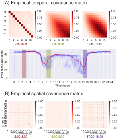
Figure 1: Empirical results based on forecasting results from Graph Wavenet (Wu et al., 2019) with PEMS-BAY data, which consists of 325 sensors and 12-step prediction with 5-minute interval (i.e., 1 hour prediction). (A) temporal (i.e., over different prediction horizons) covariance matrices of 6th sensor 6 at different time-of-days (2:00-3:00, 8:00-9:00, and 17:00-18:00). The values are normalized with the maximum value in the diagonal entries. If the errors are temporally independent and isotropic, the covariance matrix should be a diagonal matrix. Blue lines in the speed plot represent speed observations of weekdays in test data, and the red line represents the average of weekday forecasting. The red box represents 2:00-3:00, the green box represents 8:00-9:00, and the purple box represents 17:00-18:00. (B) spatial (i.e., over different sensors) covariance matrices of 12-step-ahead prediction at different time-of-days (2:00-3:00, 8:00-9:00, and 17:00-18:00). The values are normalized with the maximum value in the diagonal entries. If the errors are spatially independent and isotropic, the covariance matrix should be a diagonal matrix.

In this study, we propose to model the forecasting errors with time-varying distribution to consider the spatiotemporal correlation, and directly train the model by maximizing the likelihood function. Specifically, we use a dynamic (i.e., time-varying) mixture density network as a flexible structure by allowing the full covariance matrix to capture the spatiotemporal dependencies. The fundamental challenge in this approach is the high computational cost due to the large $NQ\times NQ$ spatiotemporal covariance matrix for the forecasting error, where $N$ is the number of sensors and $Q$ is the forecasting horizon. To address this, we reparameterize the covariance in each mixture component as a Kronecker product of two separate spatial and temporal covariance matrices. In order to efficiently learn the covariance matrix in the deep learning model, we parameterize the spatial and temporal covariance matrices using the Cholesky factorization of the precision matrices (inverse of the covariance matrix). Overall, the proposed method can be seamlessly integrated into existing deep-learning frameworks with only a few additional parameters to be learned.

2 Related Works

There are mainly two approaches to model time-varying probabilistic distribution in statistics and machine learning.

The first approach aims to model time-varying covariance matrix to capture dynamicity and spatiotemporal correlation. One method is the Wishart process (Wilson & Ghahramani, 2010), which is a stochastic process that models the time-varying covariance matrix of a multivariate time series. Another popular method is the GARCH (Generalized Autoregressive Conditional Heteroskedasticity) model (Bauwens et al., 2006), which have been widely used to model the time-varying variances of time series data, especially widely used for the finance data. GARCH models assume that the variance of the errors is a function of past errors, allowing for the capture of dynamic volatility patterns. Moreover, recent studies combining statistical approaches with deep learning also align in this category. Salinas et al. (2020) proposed DeepAR to produce probabilistic forecasting for time-series. The given neural network outputs the parameters of Gaussian distribution (the mean and the variance), and multiple time-series could be trained jointly with shared covariates. Salinas et al. (2019) employed a Gaussian copula with a low-rank structure for time-varying covariance learning with neural networks. However, these models assume that the distribution of the errors follows a unimodal distribution, while the distribution may be multimodal for spatiotemporally correlated errors.

Another approach is to use a mixture of distributions focusing on multimodality. One example is Wong & Li (2000) which proposed the Mixture Autoregressive (MAR) model to model non-linear time series by using a mixture of Gaussian autoregressive components. Also, a series of works use the Mixture Density Network (MDN) (Bishop, 1994) by combining the mixture idea with neural networks. Nikolaev et al. (2013) presented the recurrent mixture density network combined with GARCH (RMDN-GARCH) for time-varying conditional density estimation. Ellefsen et al. (2019) also analyzed the prediction generated by mixture density recurrent neural networks (MD-RNN) and tested the ability to capture multimodality by using the mixture density network. However, these studies usually use MDN to model univariate time series prediction; even if they model multivariate time series prediction and spatiotemporal forecasting, they assume a diagonal covariance matrix and only predict the variances. This setting represents that there is no correlation between forecasting errors.

Our idea is to leverage the advantages of both approaches while keeping the model scalable to train without heavy computation. We use a dynamic mixture of zero-mean Gaussian distribution to characterize the distribution of forecasting errors, where the mixture weight is time-varying, while the covariance matrices in component distributions are fixed. Also, we propose a decomposition method using the Kronecker product to keep the scalability without further assuming the characteristics (such as low-rank-ness as in Salinas et al. (2019)) of the covariance matrix.

3 Methodology

3.1 Background

First, we briefly give out the formulation of the problem, i.e., short-term traffic speed forecasting. Given a time window $t$, we denote by $v_{t}^{n}$ the average speeds of the $n$-th sensor. The speed observations in the whole network at the given time window are denoted by vector $\mathbf{x}_{t}=\left[v_{t}^{1},v_{t}^{2},\cdots,v_{t}^{N}\right]^{\top}\in\mathbb{R}^{N}$. Given the $P$ historical observations ${X}_{t}=\left[\mathbf{x}_{t-P+1},\cdots,\mathbf{x}_{t}\right]\in\mathbb{R}^{N\times P}$, we aim to predict the speed of $N$ sensors for the next $Q$ steps, i.e., ${Y}_{t}\in\mathbb{R}^{N\times Q}$ as a spatiotemporal speed matrix.

Conventional training of deep-learning models for short-term traffic speed forecasting problems can be regarded as learning of a mean-prediction function $f_{M}$ by minimizing MSE or MAE loss ($\mathcal{L}_{\text{MSE/MAE}}$):

$$\begin{split}&f^{*}_{M}=\arg\min_{f_{M}}\mathcal{L}_{\text{MSE/MAE}}\\ &\mathcal{L}_{\text{MSE/MAE}}=\begin{cases}&\|Y_{t}-M_{t}\|^{2}_{F}\quad\textrm{for MSE},\\ &\|Y_{t}-M_{t}\|_{1}\quad\textrm{for MAE},\\ \end{cases}\\ \end{split}$$ (1)

where $M_{t}=f_{M}(X_{t})\in\mathbb{R}^{N\times Q}$ is a matrix of the expected future traffic speed. The convention of using MSE loss for training deep learning models for traffic speed forecasting assumes that the error, $R_{t}=Y_{t}-M_{t}\in\mathbb{R}^{N\times Q}$, follows a zero-mean Gaussian distribution with isotropic noise:

$$\begin{split}\operatorname{vec}({R}_{t})\sim\mathcal{N}(0,{\Sigma=\sigma^{2}I_{NQ}}),\end{split}$$ (2)

3.2 Learning Spatiotemporal Error Distribution with Dynamic Mixture

In this study, we aim to model the distribution of forecasting error, and train a given deep-learning-based traffic forecasting model with a redesigned loss function. We use a dynamic mixture of zero-mean Gaussian distribution, where only the mixture weights are time-varying. Also, we explicitly model the distribution of error with spatiotemporal correlation and directly train the model by using the following loss function:

$$\begin{split}&\mathcal{L}=(1-\rho)\mathcal{L}_{\text{MSE/MAE}}+\rho\mathcal{L}_{\text{NLL}},\\ &\mathcal{L}_{\text{NLL}}=-\log p\left(R_{t}\right),\end{split}$$ (3)

where $\mathcal{L}_{\text{NLL}}$ is the negative log-likelihood of the forecasting errors and $\rho$ is the weight parameter.

One intuitive and interpretable solution to model a complex multivariate distribution is to use a mixture of Multivariate Gaussian distributions, which can represent or approximate practically any distribution of interest while being intuitive and easy to handle (Bishop, 1994; Hara et al., 2018). Furthermore, we use a dynamic mixture of multivariate zero-mean Gaussian distribution with a full covariance matrix to model the distribution of spatiotemporally correlated errors and assume that the probability density function of the error can be formulated as a mixture of $K$ multivariate zero-mean Gaussian with dynamic (i.e., time-varying) mixture weights $\omega^{k}_{t}$:

$$\operatorname{vec}\left({R}_{t}\right)\sim\sum_{k=1}^{K}\omega_{t}^{k}\cdot\mathcal{N}\left({0},\Sigma^{k}\right),$$ (4)

where ${\Sigma^{k}}\in\mathbb{R}^{NQ\times NQ}$ is the time-independent spatiotemporal covariance matrix for $k$-th component, and $\omega_{t}^{k}\geq 0$ is the time-varying weight (proportion) for $k$-th covariance matrix, which should be sum to 1, i.e., $\sum_{k=1}^{K}\omega_{t}^{k}=1$, for any $t$. Here, note that the mixture weight, $\omega_{t}^{k}$, is time-dependent (or input-dependent; $\omega_{t}^{k}=f_{\omega}(X_{t})$), while the covariance matrix in the component distribution $\Sigma^{k}$ is not. This representation allows modeling the time-varying distribution of error distribution while remaining intuitive and interpretable by analyzing the component distribution.

However, this approach has a critical issue in computing the log-likelihood of this distribution, which requires high computation cost due to the large size of ${\Sigma^{k}}$ (i.e., $NQ\times NQ$). Directly learning such a large spatiotemporal covariance matrix (${\Sigma^{k}}\in\mathbb{R}^{NQ\times NQ}$) is infeasible when $N$ or $Q$ becomes large, since computing the negative log-likelihood involves calculating the inverse and the determinant of the covariance matrix. For example, the widely-used PEMS-BAY traffic speed data consists of observations from 325 sensors, and the forecasting horizon is usually set to 1 hour (i.e., 12 timesteps with a 5-minute interval). This would result in $N=325$ and $Q=12$, and the size of $\Sigma^{k}$ becomes ${3900\times 3900}$.

To address the scalability issue, we propose a decomposition method that parameterizes each $\Sigma^{k}$ as a Kronecker product of spatial covariance matrix $\Sigma_{N}^{k}$ and temporal covariance matrix $\Sigma_{Q}^{k}$:

$$R_{t}\sim\sum_{k=1}^{K}\omega_{t}^{k}\cdot\mathcal{N}\left({0},\Sigma^{k}=\Sigma^{k}_{Q}\otimes\Sigma^{k}_{N}\right),$$ (5)

where $\Sigma^{k}_{N}\in\mathbb{R}^{N\times N}$ and $\Sigma^{k}_{Q}\in\mathbb{R}^{Q\times Q}$ are spatial and temporal covariance for the $k$-th component. This representation is equivalent to assuming the error $R_{t}$ follows a dynamic mixture of zero-mean matrix normal distribution:

$$R_{t}\sim\sum_{k=1}^{K}\omega_{t}^{k}\cdot\mathcal{MN}({0},\Sigma^{k}_{N},\Sigma^{k}_{Q}),$$ (6)

where $\mathcal{MN}$ represents a zero-mean matrix normal distribution with probability density function:

$$\begin{split}&p^{k}_{MN}(X|{0},\Sigma^{k}_{Q},\Sigma^{k}_{N})=\frac{\exp{\left(-\frac{1}{2}\operatorname{Tr}\left[{(\Sigma^{k}_{Q})}^{-1}{X}^{\top}{(\Sigma^{k}_{N})}^{-1}{X}\right]\right)}}{(2\pi)^{NQ/2}|\Sigma^{k}_{Q}|^{N/2}|\Sigma^{k}_{N}|^{Q/2}}.\end{split}$$ (7)

Then, the NLL loss can be calculated as:

$$\mathcal{L}_{\text{NLL}}$$ (8)

$$=-\log p\left(R_{t}\right) =-\log\sum_{k=1}^{K}\omega_{t}^{k}\cdot p^{k}_{MN}\left(R_{t}\,|\,{0},\Sigma^{k}_{N},\Sigma^{k}_{Q}\right)$$

$$=-\log\sum_{k=1}^{K}\exp \Bigg{(}\log\omega^{k}_{t}-\frac{NQ}{2}\log(2\pi)$$

$$+N\log|\Sigma_{Q}^{k}|^{-\frac{1}{2}}+Q\log|\Sigma_{N}^{k}|^{-\frac{1}{2}}$$

$$-\frac{1}{2}\operatorname{Tr}\left[{(\Sigma_{Q}^{k})}^{-1}{R_{t}}^{\top}{(\Sigma_{N}^{k})}^{-1}{R_{t}}\right]\Bigg{)}.$$

Figure 2: The model training with (a) conventional MSE/MAE loss and with (b) the proposed method.

For ease of computation, we can further parameterize $\Sigma^{k}_{N}$ and $\Sigma^{k}_{Q}$ using the Cholesky factorization of the precision (inverse of covariance) matrices, $\Lambda^{k}_{N}$ and $\Lambda^{k}_{Q}$:

$$\begin{split}&{(\Sigma^{k}_{N})}^{-1}=\Lambda^{k}_{S}=L^{k}_{N}{L^{k}_{N}}^{\top},\\ &{(\Sigma^{k}_{Q})}^{-1}=\Lambda^{k}_{Q}={L^{k}_{Q}}{L^{k}_{Q}}^{\top},\\ &\log|\Sigma_{N}^{k}|^{-\frac{1}{2}}=\log\left|\Lambda^{k}_{N}\right|^{\frac{1}{2}}=\sum_{n=1}^{N}\log[L^{k}_{N}]_{n,n},\\ &\log|\Sigma_{Q}^{k}|^{-\frac{1}{2}}=\log\left|\Lambda^{k}_{Q}\right|^{\frac{1}{2}}=\sum_{q=1}^{Q}\log[L^{k}_{Q}]_{q,q}.\\ \end{split}$$ (9)

where $L^{k}_{N}$ and $L_{Q}^{k}$ are the $k$-th spatial and temporal Cholesky factors (i.e., lower triangular matrices with positive diagonal entries), respectively. The advantage of using the parameterization in Eq. (9) is that we can avoid inverse operation during training, since it is hard to guarantee the invertibility of a matrix during the training process. During implementation, we found that directly parameterizing with covariance matrices can result in divergence of the loss function, gradient exploding, and singular (non-invertible) covariance matrix. We resolved these issues by parameterizing the precision matrix. Since we do not have to invert the matrix during training, the training process is much more stable than parameterizing the covariance matrix using Cholesky factorization. Also, initializing the Cholesky factors as diagonal matrices helped stabilize the training process as well. Also, we can avoid computing inverse operations during the training and efficiently compute the determinant by summing the logarithms of diagonal entries in the Cholesky factor.

Also, the trace term can be simplified into computing the square of Frobenius Norm of $Z_{t}^{k}={(L^{k}_{N})}^{\top}R_{t}^{k}{L^{k}_{Q}}$ as

$$\begin{split}\operatorname{Tr}\left[\Lambda^{k}_{Q}{(R_{t}^{k})}^{\top}\Lambda^{k}_{N}R_{t}^{k}\right]&=\operatorname{Tr}\left[{L^{k}_{Q}}{(L^{k}_{Q})}^{\top}{(R_{t}^{k})}^{\top}{L^{k}_{N}}{(L^{k}_{N})}^{\top}R_{t}^{k}\right]\\ &=\operatorname{Tr}\left[Z_{t}^{k}{(Z_{t}^{k})}^{\top}\right]=\|Z_{t}^{k}\|_{F}^{2}.\end{split}$$ (10)

Finally, Eq. (8) can be simplified into

$$\mathcal{L}_{\text{NLL}}=$$ (11)

$$-\log\sum_{k=1}^{K}\exp \Big{(}\log\omega^{k}_{t}-\frac{NQ}{2}\log(2\pi)-\frac{1}{2}\|Z_{t}^{k}\|_{F}^{2}$$

$$+N\sum_{q=1}^{Q}\log[L^{k}_{Q}]_{q,q}+N\sum_{n=1}^{N}\log[L^{k}_{N}]_{n,n}\Big{)}.$$

Note the term inside exponential function may become very large (either negative or positive), and this will make it infeasible to compute the log-likelihood. To avoid numerical problems in the training process, we use the Log-Sum-Exp trick $\log\sum_{k=1}^{K}\exp(z_{k})=z^{*}+\log\sum_{k=1}^{K}\exp(z_{k}-z^{*})$ with $z^{*}=\max\{z_{1},\cdots,z_{K}\}$.

Finally, we can train a given baseline model based on Eq. (3) by using both conventional MSE/MAE loss ($\mathcal{L}_{\text{MSE/MAE}}$) as well as the NLL loss ($\mathcal{L}_{\text{NLL}}$). We jointly train $f_{M}$, $f_{\omega}$, $L_{Q}^{k}$, and $L^{k}_{N}$ by minimizing the total loss ($\mathcal{L}=\mathcal{L}_{\text{MSE/MAE}}+\rho\mathcal{L}_{\text{NLL}}$). Both $f_{M}$ and $f_{\omega}$ are represented as a neural network. We slightly change the last layer of the baseline model to output a hidden representation of the given input, and we use two separate Multi-layer Perceptron (MLP) for $f_{M}$ and $f_{\omega}$ as shown in Figure 2. In other words, the baseline model is a shared layer for $f_{M}$ and $f_{\omega}$ to calculate a hidden representation of the input, and the last MLP is the function-specific module to calculate the desired output. We do not have an activation function at the last layer of MLP for $f_{M}$ since we generally use z-score normalization before feeding the input to the model, but we apply the softmax function at the last layer of MLP for $f_{\omega}$ to force it to be summed to 1. The gradient updates of $L_{Q}^{k}$ and $L^{k}_{N}$ are only applied to the “lower” part of the matrices, and the values in the upper parts remain as 0 during the whole process. In parameter initialization, we initialized both $L_{Q}^{k}$ and $L_{N}^{k}$ as a diagonal matrix, which was empirically more stable than random initialization.

Table 1: Summary of results. The best result in each column is bolded with a star mark

Data	Model	RMSE				MAPE				MAE
		15 min	30 min	45 min	60 min	15 min	30 min	45 min	60 min	15 min	30 min	45 min	60 min
PEMS-BAY	GWN	2.57	3.36	3.76	4.05	2.86	3.81	4.36	4.75	1.39	1.76	1.98	2.15
	+$\mathcal{L}_{\text{NLL}}$(1)	2.56	3.40	3.79	4.02	2.88	3.87	4.37	4.71	1.35	1.70	1.88	2.01
	+$\mathcal{L}_{\text{NLL}}$(2)	*2.54	3.34	3.69	*3.88	*2.83	3.79	4.25	4.55	*1.34	*1.68	1.86	*1.97
	+$\mathcal{L}_{\text{NLL}}$(3)	*2.54	*3.32	*3.68	*3.88	*2.83	3.77	4.27	4.61	*1.34	*1.68	*1.85	*1.97
	+$\mathcal{L}_{\text{NLL}}$(5)	2.55	3.34	3.71	3.92	2.85	*3.73	*4.21	*4.50	1.35	1.68	1.86	1.98
	STGCN	3.83	4.32	4.60	4.85	5.51	6.03	6.39	6.65	2.36	2.59	2.73	2.84
	+$\mathcal{L}_{\text{NLL}}$(1)	2.84	3.71	4.21	4.58	3.56	4.93	5.86	6.68	1.64	2.07	2.35	2.59
	+$\mathcal{L}_{\text{NLL}}$(2)	*2.78	3.57	4.00	4.33	3.54	4.72	5.39	5.93	1.63	2.03	2.28	2.49
	+$\mathcal{L}_{\text{NLL}}$(3)	2.80	*3.56	*3.99	*4.31	*3.50	*4.52	*5.14	*5.66	*1.62	*1.99	*2.23	*2.42
	+$\mathcal{L}_{\text{NLL}}$(5)	2.81	3.62	4.11	4.49	3.49	4.55	5.31	5.96	1.63	2.02	2.29	2.53
METR-LA	GWN	5.05	5.90	6.44	6.85	7.47	9.01	10.02	10.78	2.90	3.36	3.68	3.93
	+$\mathcal{L}_{\text{NLL}}$(1)	4.95	5.94	6.53	6.88	7.16	8.77	9.76	10.44	2.84	3.32	3.65	*3.87
	+$\mathcal{L}_{\text{NLL}}$(2)	4.94	5.93	6.52	6.95	*7.13	*8.68	9.69	10.39	*2.81	*3.30	*3.62	3.89
	+$\mathcal{L}_{\text{NLL}}$(3)	4.97	5.95	6.52	6.92	7.14	8.72	*9.66	*10.32	2.84	3.34	3.65	3.91
	+$\mathcal{L}_{\text{NLL}}$(5)	*4.93	*5.85	*6.42	*6.81	7.26	8.81	9.87	10.71	2.86	3.34	3.65	3.93
	STGCN	6.61	7.86	8.63	9.53	9.56	11.62	13.36	15.40	3.89	4.61	5.26	6.09
	+$\mathcal{L}_{\text{NLL}}$(1)	*5.95	*6.57	*6.95	*7.18	*9.03	*10.51	*11.53	*12.43	*3.65	*4.11	*4.44	*4.65
	+$\mathcal{L}_{\text{NLL}}$(2)	6.32	7.22	7.78	8.02	9.39	11.24	12.53	13.34	3.85	4.55	5.05	5.27
	+$\mathcal{L}_{\text{NLL}}$(3)	6.12	6.80	7.19	7.42	9.47	11.20	12.26	13.24	3.78	4.30	4.64	4.88
	+$\mathcal{L}_{\text{NLL}}$(5)	6.08	6.74	7.15	7.38	9.37	10.82	11.82	12.58	3.78	4.28	4.64	4.86

3.3 Discussion

The proposed model aims to effectively deal with spatiotemporally correlated errors by modeling the time-varying distribution of the spatiotemporal matrix process. By utilizing a probabilistic sequence-to-sequence forecasting model, we are able to characterize the error process with a predictable distribution. This enables us to predict both the mean and the error distribution, providing a more comprehensive forecasting model.

One of the key advantages of the proposed model is its ability to handle errors with a multimodal structure. By utilizing a mixture model, we are able to model the multimodal distribution and offer interpretability for the different modes present in the errors. This is particularly useful in situations where there are multiple potential outcomes or patterns (i.e., multimodality) present in the errors. This feature allows the proposed model to be more robust to the complex and diverse nature of spatiotemporal data.

The proposed model also stands out for being a special case of a matrix-variate Mixture Density Network. This architecture allows us to handle the complexities of spatiotemporal data by leveraging the matrix-variate nature of the data, resulting in a more nuanced and accurate forecasting model. The proposed model does not output the Cholesky factors (i.e., $L_{N}^{k}$ and $L_{Q}^{k}$), while previous studies using a mixture density network either output the variances by assuming a diagonal covariance matrix or output a full covariance matrix from the base line model. The proposed approach can avoid over-fitting and offer interpretability, which is a crucial aspect in many real-world applications.

Overall, our proposed model offers a powerful approach for dealing with spatiotemporally correlated errors in a probabilistic and interpretable manner. It provides a comprehensive forecasting model that can effectively handle multimodal errors and the complexities of spatiotemporal data, while avoiding over-fitting and providing interpretability. This makes the proposed model a valuable tool for various real-world applications that deal with spatiotemporal data.

4 Experiment and Results

4.1 Data

We conduct experiments to verify the performance of the proposed model. The datasets we use are called PEMS-BAY and METR-LA, which are some of the most widely-used datasets in traffic forecasting (Li et al., 2017). PEMS-BAY was collected from the California Transportation Agencies (CalTrans) Performance Measurement System (PeMS) (Chen et al., 2001). It is collected from 325 sensors installed in the Bay Area with observations of 6 months of data ranging from January 1 to May 31, 2017. METR-LA was collected from the highway of Los Angeles County (Jagadish et al., 2014). It is collected from 207 sensors with observations of 4 months of data ranging from March 1 to June 30, 2012. Both datasets register the average traffic speed of sensors with a 5-min resolution.

4.2 Performance Metric

We choose Root Mean Square Error (RMSE), Mean Absolute Percentage Error (MAPE), and Mean Absolute Error (MAE) of speed prediction at 15, 30, 45, and 60 minutes ahead as key metrics to evaluate forecasting accuracy, corresponding to 3-, 6-, 9-, and 12-step-ahead prediction, respectively.

4.3 Model Configuration

The proposed method can work as an add-on to any type of traffic forecasting model based on deep learning. We use Graph Wavenet (GWN) (Wu et al., 2019) and Spatio-Temporal Graph Convolutional Networks (STGCN) (Yu et al., 2017) as our baseline models. Following the conventional configurations, we aim to predict 12 steps (i.e., one hour in the future) based on 12-step observation (i.e., observations from one hour in the past). We use different settings for $K$, the number of mixture components, and we denote the proposed model as $+\mathcal{L}_{\text{NLL}}$(K) where $K\in\{1,2,3,5\}$. We used $\rho=0.001$ based on exhaustive hyperparameter tuning.

4.4 Results

Table 1 shows the summary of results. We use Mean Squared Error (MSE) as the base loss function ($\mathcal{L}_{\text{MSE/MAE}}$), and the results based on MAE as the base loss function is presented in Appendix A. We can observe that the proposed method consistently shows improvements for forecasting accuracy regardless of the dataset, base loss, and performance metrics. The performance improvement rate is larger in the longer forecasting horizon (60 min) than that in the shorter forecasting horizon (15 min). This is intuitive that we usually have stronger spatiotemporal correlation at longer forecasting horizons than shorter forecasting horizons. Especially, it is notable that applying the proposed method improves the performance of MAPE since MAPE penalizes large errors in congested traffic states (when speed is low). Most of the correlated errors occur when the traffic state is in a congested state (Li et al., 2022), while the errors in a free flow state usually follow independent Gaussian distribution.

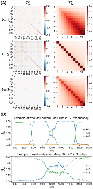
Figure 3: (A) Learned spatial ($\Sigma_{N}^{k}$) and temporal ($\Sigma_{Q}^{k}$) covariance matrices with $K=3$. For better visualization, we normalized the temporal covariance matrix by dividing the temporal covariance matrices by the maximum value of the diagonal entries in temporal covariance matrices and multiplied the same value to the spatial covariance matrices, since the Kronecker product has the scale-invariant property, i.e., $A\otimes B=\left(\nu A\right)\otimes\left(\frac{1}{\nu}B\right)$. (B) Examples of patterns of the mixture weight $\omega_{t}^{k}$. There were two distinct patterns for 35 days in the testing dataset, which could be categorized into weekday-pattern and weekend-pattern. The representative cases for each category are shown.

One advantage of using the proposed method is that representing the error distribution with the dynamic mixture distribution offers an interpretable framework for traffic speed forecasting. We selected $K=3$ with MSE base loss on PEMS-BAY dataset using GWN model for this test. Figure 3 (A) shows the learned spatial and temporal covariance matrices. We can observe the spatial correlation structure of the errors in each mixture component, and the spatial structure is more clear in the first component. The temporal covariance matrices show an increasing tendency of variance/covariance as the forecasting time horizon increases. This is intuitive since the variance of the forecasting increases at a longer forecasting timestep, and we can verify that the proposed method enables learning this type of characteristic of traffic speed forecasting. Also, the learned spatial precision matrices show sparse structure, which aligns well with the underlying road network. A more detailed discussion is presented in Appendix B.

Figure 3 (B) shows the change of $\omega_{t}^{k}$ over different time-of-day. The x-axis is the time-of-day ranging from 0:00 to 23:55 with 5-minute-interval, and the y-axis is the value for $\omega_{t}^{k}$. It is important to note that the sum of $\omega_{t}^{k}$ should equal to 1 at each time-of-day. During examining this result, we found that there are two distinct patterns in 35 days of data in testing dataset. Surprisingly and trivially, these two patterns can be classified as weekday and weekend patterns. The upper figure shows the representative example of weekday pattern from Wednesday, May 10th, 2017, while the lower figure shows the representative example of weekend pattern from Sunday, May 28th, 2017. In both cases, the the pattern in the first mixture component ($k=1$) is represented by the blue line and the the pattern in the third component ($k=3$) pattern is represented by the green line and are the main components, and the influence of the second mixture component is small in both cases. In the weekday pattern, the pattern in the first mixture component is mainly dominant during peak hour periods including both morning peak (from 6:00 to 9:00) and afternoon peak (from 15:00 to 19:00) and the pattern in the third mixture component is mainly dominant during night-time from 21:00 to 5:00. In the afternoon off-peak, a mixture of the two patterns is observed. When interpreting these results together with the results of Figure 3 (A), it can be seen that the results in spatial and temporal covariance matrices of the first component show a stron spatial and temporal correlation, which can be easily interpreted as “peak-hour pattern.” On the other hand, in the third component, the temporal correlation is strong, but the spatial covariance is almost diagonal matrix, representing that the speed observations are spatially independent, which can be interpreted as “off-peak pattern.” We have a mixture of two patterns in the afternoon off-peak hours since the distribution cannot be represented as unimodal distribution since there may or may not be congestion in some occasion. As a result, a mixture of peak-hour pattern and off-peak pattern is suitable for this time period. The weekend pattern shows a different pattern from the weekday pattern in that, at night time, it is similar to the weekday pattern with third mixture component dominant, but during the day time, it is represented as a mixture of first and the third mixture component, similar to the weekday’s afternoon off-peak hours.

5 Conclusion

This study proposes a scalable and efficient way to learn the time-varying and multimodal distribution for traffic forecasting errors. The proposed method characterizes the distribution of error as a dynamic mixture of zero-mean Gaussian distributions with full covariance matrices in the component distribution. The $NQ\times NQ$ spatiotemporal covariance matrix for each component is decomposed as a Kronecker product of an $N\times N$ spatial covariance matrix and a $Q\times Q$ temporal covariance matrix. The proposed method can be seamlessly integrated into existing deep-learning models for traffic forecasting as an add-on module. The proposed method is tested using two widely-used traffic forecasting models, GWN and STGCN. The results show that the proposed method can improve forecasting accuracy. Also, the proposed method offers an interpretable framework to understand the traffic pattern by analyzing the learned parameters in the dynamic mixture model.

The proposed method can be extended to other applications where there is a complex high-dimensional correlation in a time-varying manner. In particular, it can be useful to model the prediction error for wind speed forecasting and climate forecasting, since there exists an even larger multi-dimensional covariance matrix. The scalable solution proposed in this study is expected to be effective in addressing this challenge.

Appendix A Result using MAE as the Base Loss

Table 2: Summary of results. The best result in each column is bolded with a star mark

Data	Model	RMSE				MAPE				MAE
		15 min	30 min	45 min	60 min	15 min	30 min	45 min	60 min	15 min	30 min	45 min	60 min
PEMS-BAY	GWN	2.65	3.46	3.87	4.20	2.82	3.80	4.38	4.81	1.36	1.72	1.93	2.10
	+$\mathcal{L}_{\text{NLL}}$(1)	2.53	3.33	3.70	3.89	2.83	3.76	4.25	4.56	1.35	1.70	1.87	1.99
	+$\mathcal{L}_{\text{NLL}}$(2)	*2.52	3.29	3.68	3.92	2.80	3.72	4.24	4.62	1.33	*1.66	1.85	1.99
	+$\mathcal{L}_{\text{NLL}}$(3)	*2.52	*3.28	*3.65	*3.88	*2.76	*3.69	4.21	4.56	*1.32	*1.66	*1.84	*1.97
	+$\mathcal{L}_{\text{NLL}}$(5)	2.53	3.32	3.70	3.91	2.76	3.68	*4.17	*4.52	1.34	1.68	1.87	1.99
	STGCN	3.45	4.14	4.75	5.29	4.52	5.27	6.10	6.97	2.03	2.32	2.62	2.92
	+$\mathcal{L}_{\text{NLL}}$(1)	2.90	3.83	4.35	4.74	3.73	5.20	6.12	6.92	1.71	2.17	2.45	2.70
	+$\mathcal{L}_{\text{NLL}}$(2)	3.02	3.88	4.36	4.71	4.23	5.51	6.32	7.01	1.78	2.20	2.46	2.70
	+$\mathcal{L}_{\text{NLL}}$(3)	*2.83	*3.66	*4.15	*4.51	3.55	4.73	5.54	6.26	1.64	*2.03	*2.29	*2.52
	+$\mathcal{L}_{\text{NLL}}$(5)	*2.83	3.69	4.18	4.55	*3.42	*4.61	*5.44	*6.17	*1.63	2.04	2.30	2.54
METR-LA	GWN	5.12	6.05	6.66	7.16	7.21	8.60	9.47	*10.17	*2.78	*3.21	*3.51	3.76
	+$\mathcal{L}_{\text{NLL}}$(1)	5.02	6.00	6.59	6.94	*6.98	8.46	*9.46	10.31	2.86	3.30	3.59	3.83
	+$\mathcal{L}_{\text{NLL}}$(2)	*4.98	*5.93	*6.51	*6.87	7.05	8.60	9.58	10.27	*2.78	3.22	*3.51	*3.72
	+$\mathcal{L}_{\text{NLL}}$(3)	4.99	6.00	6.62	6.98	6.99	8.53	9.53	10.29	*2.78	3.24	3.56	3.78
	+$\mathcal{L}_{\text{NLL}}$(5)	4.96	5.98	6.55	6.89	6.99	*8.44	9.47	10.36	2.87	3.30	3.59	3.83
	STGCN	6.43	7.93	8.94	10.08	9.04	11.11	12.78	14.82	*3.53	4.30	5.00	5.90
	+$\mathcal{L}_{\text{NLL}}$(1)	*6.14	*6.94	*7.39	*7.52	*8.76	*10.34	*11.38	*12.06	3.71	* 4.29	*4.66	*4.80
	+$\mathcal{L}_{\text{NLL}}$(2)	6.55	7.61	8.30	8.49	9.36	11.45	12.93	13.77	3.86	4.67	5.25	5.45
	+$\mathcal{L}_{\text{NLL}}$(3)	6.24	7.22	7.86	8.03	8.89	10.73	12.06	12.96	3.74	4.45	4.97	5.16
	+$\mathcal{L}_{\text{NLL}}$(5)	6.21	7.12	7.65	7.80	9.21	11.00	12.31	13.13	3.74	4.39	4.83	4.97

Appendix B Learned Precision Matrix

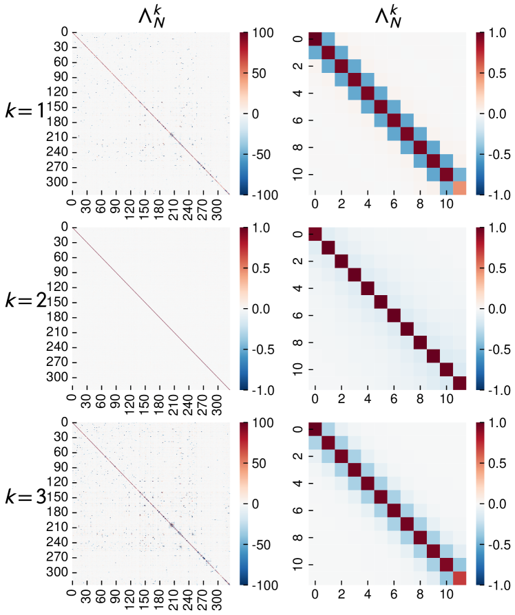
Figure 4: Learned spatial ($\Lambda_{N}^{k}$) and temporal ($\Lambda_{Q}^{k}$) precision matrices with $K=3$. For better visualization, we normalized the temporal precision matrix by dividing the temporal precision matrices by the maximum value of the diagonal entries in temporal precision matrices and multiplied the same value to the spatial precision matrices, since the Kronecker product has the scale-invariant property, i.e., $A\otimes B=\left(\nu A\right)\otimes\left(\frac{1}{\nu}B\right)$.

The results of learned precision matrix results provide a deeper understanding of the spatiotemporal relationships in traffic forecasting. The spatial precision matrix shows a sparse structure, indicating that the underlying data structure is a graph. This aligns well with the road network, as the sparse structure corresponds to the connections between different roads in the network. Furthermore, the temporal precision matrix shows a first-order relationship, which is intuitive as it implies that the temporal dependencies in the data can be modeled as a first-order graph. This indicates that the proposed method effectively captures the underlying road network structure and temporal dependencies in the traffic speed forecasting data.

We also can find that the distribution of the traffic speed data can be modeled by using the sparsity of the precision matrix. This is a well-known property of Gaussian Markov Random Fields (GMRF) (Rue & Held, 2005). As a future work, it could be proposed to use GMRF by incorporating the road network structure and first-order temporal relationship. This approach would allow for more accurate modeling of the dependencies between different roads in the network. Additionally, an underlying spatiotemporal graph could also be assumed to directly model the sparse spatiotemporal precision ($\Lambda^{k}\in\mathbb{R}^{NQ\times NQ}$) without assuming a matrix normal distribution. This approach could provide further insights into the relationships between traffic speeds at different locations and at different times.

References

- Bauwens et al. (2006) Bauwens, L., Laurent, S., and Rombouts, J. V. Multivariate garch models: a survey. Journal of applied econometrics, 21(1):79–109, 2006.
- Bishop (1994) Bishop, C. M. Mixture density networks. 1994.
- Cai et al. (2020) Cai, L., Janowicz, K., Mai, G., Yan, B., and Zhu, R. Traffic transformer: Capturing the continuity and periodicity of time series for traffic forecasting. Transactions in GIS, 24(3):736–755, 2020.
- Chen et al. (2001) Chen, C., Petty, K., Skabardonis, A., Varaiya, P., and Jia, Z. Freeway performance measurement system: mining loop detector data. Transportation Research Record, 1748(1):96–102, 2001.
- Ellefsen et al. (2019) Ellefsen, K. O., Martin, C. P., and Torresen, J. How do mixture density rnns predict the future? arXiv preprint arXiv:1901.07859, 2019.
- Hara et al. (2018) Hara, Y., Suzuki, J., and Kuwahara, M. Network-wide traffic state estimation using a mixture gaussian graphical model and graphical lasso. Transportation Research Part C: Emerging Technologies, 86:622–638, 2018.
- Jagadish et al. (2014) Jagadish, H. V., Gehrke, J., Labrinidis, A., Papakonstantinou, Y., Patel, J. M., Ramakrishnan, R., and Shahabi, C. Big data and its technical challenges. Communications of the ACM, 57(7):86–94, 2014.
- Li et al. (2022) Li, G., Knoop, V. L., and van Lint, H. Estimate the limit of predictability in short-term traffic forecasting: An entropy-based approach. Transportation Research Part C: Emerging Technologies, 138:103607, 2022.
- Li et al. (2015) Li, L., Su, X., Zhang, Y., Lin, Y., and Li, Z. Trend modeling for traffic time series analysis: An integrated study. IEEE Transactions on Intelligent Transportation Systems, 16(6):3430–3439, 2015.
- Li et al. (2017) Li, Y., Yu, R., Shahabi, C., and Liu, Y. Diffusion convolutional recurrent neural network: Data-driven traffic forecasting. arXiv preprint arXiv:1707.01926, 2017.
- Nikolaev et al. (2013) Nikolaev, N., Tino, P., and Smirnov, E. Time-dependent series variance learning with recurrent mixture density networks. Neurocomputing, 122:501–512, 2013.
- Rue & Held (2005) Rue, H. and Held, L. Gaussian Markov random fields: theory and applications. Chapman and Hall/CRC, 2005.
- Salinas et al. (2019) Salinas, D., Bohlke-Schneider, M., Callot, L., Medico, R., and Gasthaus, J. High-dimensional multivariate forecasting with low-rank gaussian copula processes. Advances in neural information processing systems, 32, 2019.
- Salinas et al. (2020) Salinas, D., Flunkert, V., Gasthaus, J., and Januschowski, T. Deepar: Probabilistic forecasting with autoregressive recurrent networks. International Journal of Forecasting, 36(3):1181–1191, 2020.
- Wilson & Ghahramani (2010) Wilson, A. G. and Ghahramani, Z. Generalised wishart processes. arXiv preprint arXiv:1101.0240, 2010.
- Wong & Li (2000) Wong, C. S. and Li, W. K. On a mixture autoregressive model. Journal of the Royal Statistical Society: Series B (Statistical Methodology), 62(1):95–115, 2000.
- Wu et al. (2019) Wu, Z., Pan, S., Long, G., Jiang, J., and Zhang, C. Graph wavenet for deep spatial-temporal graph modeling. arXiv preprint arXiv:1906.00121, 2019.
- Yu et al. (2017) Yu, B., Yin, H., and Zhu, Z. Spatio-temporal graph convolutional networks: A deep learning framework for traffic forecasting. arXiv preprint arXiv:1709.04875, 2017.