Control of Active Brownian Particles: An exact solution

Abstract

Control of stochastic systems is a challenging open problem in statistical physics, with a wealth of potential applications from biology to granulates. Unlike most cases investigated so far, we aim here at controlling a genuinely out-of-equilibrium system, the two dimensional Active Brownian Particles model in a harmonic potential, a paradigm for the study of self-propelled bacteria. We search for protocols for the driving parameters (stiffness of the potential and activity of the particles) bringing the system from an initial passive-like steady state to a final active-like one, within a chosen time interval. The exact analytical results found for this prototypical model of self-propelled particles brings control techniques to a wider class of out-of-equilibrium systems.

Introduction — Active matter is one of the most studied and promising topics of out-of-equilibrium statistical physics Elgeti et al. (2015); Bechinger et al. (2016); Gompper et al. (2020); O’Byrne et al. (2022). Inspired by the behaviour of biological systems such as bacteria and cells, this class of problems is characterized by the presence of internal mechanisms (e.g., self-propulsion) inducing nonzero entropy production, through energy dissipation. Motility-induced phase separation Cates and Tailleur (2015); Fily and Marchetti (2012), pattern formation Digregorio et al. (2018); Farrell et al. (2012) and velocity self-alignment Caprini et al. (2020a) are typical hallmarks of the intrinsic out-of-equilibrium nature of these systems. Among the others, activity is a key future of nano-swimmers Golestanian et al. (2007), complex colloidal or bacteria dynamics Howse et al. (2007); Gejji et al. (2012), and active transport Bressloff and Newby (2013). While the engineering of such systems becomes possible O’Byrne et al. (2022), it remains a challenge to control activity in general. This demands a proper understanding of the dynamics under confinement, an important endeavour for active objects Pototsky and Stark (2012); Dauchot and Démery (2019). The present work is a step in this direction.

Several experiments have shown the possibility to tune the degree of activity of active matter Buttinoni et al. (2012); Maggi et al. (2015a); Vizsnyiczai et al. (2017); Vutukuri et al. (2020); Militaru et al. (2021). In Ref. Buttinoni et al. (2012), for instance, silica spheres of a few $\mu m$ radius, partly covered by chromium and gold (Janus particles) are diluted in a binary mixture of water and 2,6-lutidine, that reacts with the surface of the particles and induces self-propulsion. The reaction is tuned by the intensity of light, so that the persistent velocity can be controlled. This light-dependent tuning is a promising mechanism for the control of active fluids and may have useful applications, e.g., for the clogging/unclogging of microchannels Dressaire and Sauret (2016); Caprini et al. (2020b). The main idea behind these applications is to bring the system from a passive-like to an active-like phase, and vice-versa, and to take advantage of the different distribution of the particles in the two states.

The time needed to switch the system from one phase to the other will depend, in general, on the protocol that is employed to change the values of the controlling parameters. A sudden change of the external light, for instance, may then require a long time for the relaxation of the system to the desired final distribution. It is thus important to search for protocols that allow to execute the transition in a controlled way, in a short time. This type of problems, that can be subsumed under the terminology of “swift state-to state transformations” (SST) Guéry-Odelin et al. (2023), has witnessed a surge of interest in the last 15 years. The first studies are in the realm of quantum mechanics Torrontegui et al. (2013), where they are referred to as “shortcuts to adiabaticity”; applications to statistical physics and stochastic thermodynamics are more recent Martínez et al. (2016); Guéry-Odelin et al. (2023).

In this letter, we study such SST problems for a system of Active Brownian Particles (ABP) in two dimensions Romanczuk et al. (2012); Pototsky and Stark (2012); Solon et al. (2015a, b); Basu et al. (2018, 2019); Caporusso et al. (2020). This is one of the simplest and most used models mimicking the behaviour of self-propelled particles like bacteria Romanczuk et al. (2012), whose fluctuating hydrodynamics has been shown to be equivalent to the Run-and-Tumble model describing the above mentioned Janus particles Cates and Tailleur (2013); Solon et al. (2015a). We will assume that the system is confined in an external harmonic potential with tunable stiffness, as done for instance in Ref. Takatori et al. (2016) by using acoustic waves. The stationary (steady-state) distribution of this model was found in Ref. Malakar et al. (2020). With these assumptions, we will describe a class of analytical protocols leading the system from a passive-like to an active-like state with the same stiffness in a finite time, and vice-versa. Among this class of control protocols, we will identify the one minimizing the total time required for the transition.

Model — The state of 2 dimensional ABP is defined by a spatial position $\bm{\rho}=(\rho\cos\varphi,\rho\sin\varphi)$ for the center of mass, and an angle $\theta$ associated to the orientation of the particle. The particle’s velocity is given by the sum of a self-propulsion contribution along the direction of $\theta$, $\mathbf{e}(\theta)$, with constant modulus $u_{0}$, plus a thermal Gaussian noise. The orientation $\theta$ is also subject to Gaussian fluctuations. In addition, the effect of an external potential will be taken into account. We consider the case of isotropic harmonic confinement, resulting in a force $-k\bm{\rho}$ pointing toward the origin ($k$ being the stiffness). In the overdamped limit, the time evolution is then given by the coupled Langevin equations

$$\begin{cases}\frac{d\bm{\rho}}{d\tau}=&u_{0}\widehat{\mathbf{e}}(\theta)-\mu k\bm{\rho}+\sqrt{2D_{t}}\,\bm{\xi}_{r}(\tau),\\ \frac{d\theta}{d\tau}=&\sqrt{2D_{\theta}}\,\bm{\xi}_{\theta}(\tau)\,,\end{cases}$$ (1)

where $\tau$ is the time, $\mu$ stands for the mobility, $\bm{\xi}_{r}(\tau)$ and $\bm{\xi}_{\theta}(\tau)$ are Gaussian white noises, while $D_{t}$ and $D_{\theta}$ are the translational and the rotational diffusivities.

In the following we will consider the dimensionless variables $t=D_{\theta}\tau$, $\mathbf{r}=\bm{\rho}/\Delta$, where $\Delta$ is a unit of length to be specified, and the dimensionless parameters

$$\kappa=\frac{\mu k}{D_{\theta}}\,,\quad\lambda=\frac{u_{0}}{D_{\theta}\Delta}\,,\quad\alpha=\frac{D_{\theta}\Delta^{2}}{D_{t}}\,.$$ (2)

The stationary probability density function (pdf) for this problem can be worked out analytically as a series expansion in powers of $\lambda$ Malakar et al. (2020):

$$P_{s}(r,\chi) =F(r,\chi|\kappa,\lambda,\alpha)$$ (3)

$$\equiv\alpha\sum_{m=0}^{\infty}\lambda^{m}\alpha^{m/2}\sum_{2n+|l|=m}C_{n,l}^{(m)}(\kappa)\phi_{n,l}(\sqrt{\alpha}r,\chi|\kappa)\,,$$

where $r=|\mathbf{r}|$ and $\chi=\theta-\varphi$, $\varphi$ being the orientation of the vector $\mathbf{r}$. Here, the $C_{n,l}^{(m)}$ are coefficients that can be determined by suitable recursive rules, while the explicit expression of $\phi_{n,l}$ is known Malakar et al. (2020); their definition is recalled in the Supplemental Material (SM) SM . In the following we choose $\Delta=\sqrt{D_{t}/D_{\theta}}$ as the rescaling length, so that $\alpha=1$. The stationary pdf then depends only on $\kappa$ and $\lambda$, that have the respective meaning of a dimensionless stiffness and of a normalized persistence length accounting for the degree of activity of the system.

Swift state-to-state transformations — We now face the problem of bringing the system from an initial stationary state, characterized by $\lambda=\lambda_{i}$, to a final state $\lambda=\lambda_{f}$ with the same $\kappa=\kappa_{0}$, in a given time interval $t_{f}$. Solutions obtained as sequences of stationary states (the so-called “quasi-static” protocols), where the control parameter $\lambda(t)$ is slowly varied between $\lambda_{i}$ and $\lambda_{f}$, require infinite time. They are not suitable for our purposes, since we wish to complete the connection in a given finite time $t_{f}$. Instead, we will take advantage of the known steady-state distribution (3) to look for time-dependent, non-quasi-static protocols. In particular, we search for an exact solution with functional form:

$$P(r,\chi,t)\equiv F(r,\chi|\widetilde{\kappa}(t),\widetilde{\lambda}(t),\widetilde{\alpha}(t))\,,$$ (4)

where the functions $\widetilde{\kappa}$, $\widetilde{\lambda}$ and $\widetilde{\alpha}$, yet to be specified, completely define the instantaneous state of the system (i.e., the pdf of the active particle). We introduce the tilde variables in order to make a clear distinction between the control parameters ($\kappa$ and $\lambda$) and the variables describing the state of the system ($\widetilde{\kappa}$, $\widetilde{\lambda}$ and $\widetilde{\alpha}$). The former are directly controlled during the experiments: in the proposed experimental setup, see next paragraph, they would be the (rescaled) stiffness of the external potential and the (rescaled) persistence length induced by the chosen light intensity. The tilde variables, instead, define the probability density function of the active particle at a given instant of time, which evolves in turn according to the Fokker-Planck equation defined by $\kappa$ and $\lambda$. While tilde and non-tilde variables coincide in the stationary state, they are different during a dynamic evolution.

We require $\widetilde{\kappa}(t)$, $\widetilde{\lambda}(t)$ and $\widetilde{\alpha}(t)$ to be continuous, positive functions of time such that

$$\widetilde{\kappa}(0) =\kappa_{0}\quad\quad\widetilde{\kappa}(t_{f}) =\kappa_{0}\,,$$ (5a)

$$\widetilde{\lambda}(0) =\lambda_{i}\quad\quad\widetilde{\lambda}(t_{f}) =\lambda_{f}\,,$$ (5b)

$$\widetilde{\alpha}(0) =1\quad\quad\widetilde{\alpha}(t_{f}) =1\,,$$ (5c)

so that at the beginning and at the end of the process the system is in a stationary state induced by the external parameters $\lambda_{i,f}$ and $\kappa_{0}$. In order to search for a protocol $(\kappa(t),\lambda(t))$ realizing the envisaged process, we plug the ansatz (4) into the Fokker-Planck equation for the evolution of the pdf (see SM SM for details on the calculations). It is convenient to look for solutions with constant $\widetilde{\kappa}(t)=\kappa_{0}$; with this choice, one finds that the family of solutions

$$\kappa(t) = \frac{\dot{\widetilde{\alpha}}(t)}{2\widetilde{\alpha}(t)}+\kappa_{0}\widetilde{\alpha}(t)$$ (6a)

$$\lambda(t) = \lambda_{i}\exp\left\{-\int_{0}^{t}[\kappa(t^{\prime})-\kappa_{0}]dt^{\prime}\right\}\,$$ (6b)

$$\widetilde{\kappa}(t) = \kappa_{0}\,$$ (6c)

$$\widetilde{\lambda}(t) = \lambda(t)\,,$$ (6d)

satisfies the evolution equation. The function $\widetilde{\alpha}(t)$ appearing in Eqs. (6) is arbitrary, among those that fulfill the boundary conditions (5); once it is chosen, the protocol is uniquely determined. The freedom on $\widetilde{\alpha}(t)$ provides a wide class of eligible SST for the process. This explicit solution represents our main result.

In the solution worked out, $\widetilde{\kappa}=\kappa_{0}$ is constant during the whole process. This is a relevant simplification, because it implies that the coefficients $C_{n,l}^{(m)}(\widetilde{\kappa})$ appearing in the functional form of the pdf (3) are also constant in time, and their derivatives do not appear in the calculations. By keeping $\widetilde{\kappa}$ fixed, we explore a two-dimensional manifold in the 3-dimensional space of pdf of the form (4): an even wider class of protocols may be searched for by allowing this parameter to vary in time, at the price of significantly more involved calculations.

Controlled protocols — As alluded to in the Introduction, the degree of activity and the stiffness of the external potential can be controlled in actual experiments, within parameter ranges depending on the considered setup. In order to show that the analytical results of this Letter are in principle applicable to realistic experimental situations, it is useful to recall a couple of examples. With the setup described by Buttinoni et al. Buttinoni et al. (2012), spherical Janus particles with radius $R=1\,\mu m$ can have a persistent velocity varying in the interval $0\,\mu m/s\leq u_{0}\leq 1\,\mu m/s$, depending on the intensity of the surrounding light. The rotational diffusivity has been measured to be $D_{\theta}\simeq 0.08\,s^{-1}$. By calling $\eta$ the dynamic viscosity of the fluid, $T$ the temperature and $k_{B}$ the Boltzmann constant, one gets the following equation for the translational diffusivity of the particles (not measured in the paper):

$$D_{t}=\frac{k_{B}T}{6\pi\eta R}=\frac{4}{3}R^{2}D_{\theta}\simeq 0.10\,\mu m^{2}/s\,,$$ (7)

in agreement with the estimation provided in Ref. Takatori et al. (2016) for a similar situation. The dimensionless parameter $\lambda=u_{0}/\sqrt{D_{\theta}D_{t}}$ can be thus tuned in the interval

$$0\leq\lambda\leq 11\,.$$ (8)

Slightly different results are found in Ref Buttinoni et al. (2013), corresponding to an even wider range for $\lambda$. The particles may be confined in a quasi-harmonic, controllable potential as done in Ref. Takatori et al. (2016), where acoustic waves are employed to trap a system of Janus particles with different chemical properties but similar radius. In that paper, two experimental situations are studied, in which particles with $D_{\theta}$ between $0.2s^{-1}$ and $0.5s^{-1}$ attain states with $\kappa=0.29$ and $\kappa=1.76$. Taking into account the different characteristic time for rotations, the dimensionless stiffness for the system described in Ref. Buttinoni et al. (2012) can be expected to be tunable, at least, within the interval $1.2\leq\kappa\leq 7$. A lower bound to the stiffness is expected to hold in experimental setups to prevent particles from moving away from the trap.

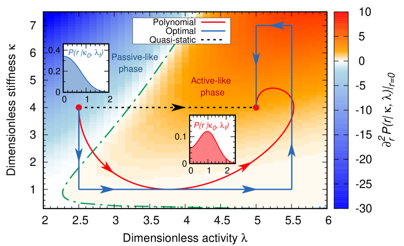
Figure 1: Parameter space of the model. The color code represents the value of $\partial_{r}^{2}P_{s}(r)|_{r=0}$, which is zero at the interface between the passive-like and the active-like phase (green dash-dotted curve). The black dotted line represents the path of a quasi-static protocol in which $\lambda$ is slowly varied between $\lambda_{i}=2.5$ and $\lambda_{f}=5$, while $\kappa=\kappa_{0}=4$ is kept constant. The red solid curve describes the solution to Eqs. (6) associated to the polynomial protocol (10); in this case the final time $t_{f}$ is chosen in such a way that $\kappa(t)$ does not exceed the bounds $1<\kappa<7$, inspired by the experimental constraints discussed in the text. The blue lines show the minimal-time protocol, the dashed branches representing instantaneous change in the control parameter $\kappa$. Plots of the position pdf for the initial and the final states are also shown.

In Fig. 1 the parameter space of the model is sketched. As in Ref. Malakar et al. (2020), we distinguish between a passive-like phase characterized by $\partial_{r}^{2}P_{s}(0,\chi)<0$ and an active-like one where the particles tend to escape from the center of the potential and $\partial_{r}^{2}P_{s}(0,\chi)>0$. The range of the control parameters that is expected to be reached in experiments includes both passive-like and active-like stationary distributions, and it is interesting to search for SST between these two states.

Possibly, the simplest way to find an explicit smooth protocol satisfying Eqs. (6) is to enforce a polynomial form for $\widetilde{\alpha}(t)$. We have to impose the boundary conditions Eq. (5c) and the final condition for $\lambda$. If we also require that

$$\kappa(0)=\kappa(t_{f})=\kappa_{0}\,,$$ (9)

i.e. that the stiffness be varied continuously without abrupt changes at the beginning and at the end of the protocol, five degrees of freedom are needed. The polynomial needs therefore to be at least fourth order, i.e.,

$$\widetilde{\alpha}(t) =1+\sum_{n=2}^{4}\widetilde{\alpha}_{n}t^{n}\quad\text{with}$$ (10)

$$\widetilde{\alpha}_{2}=-\frac{30}{\kappa_{0}t_{f}^{3}}\ln\frac{\lambda_{f}}{\lambda_{i}} ,\quad\widetilde{\alpha}_{3}=-\frac{2\widetilde{\alpha}_{2}}{t_{f}},\quad\widetilde{\alpha}_{4}=\frac{\widetilde{\alpha}_{2}}{t_{f}^{2}}\,.$$

In Fig. 1, the red solid curve shows a protocol of this sort for a realistic situation, bringing the state of the system from the passive- to the active-like phase in a time $\tau\simeq 0.66D_{\theta}^{-1}$. Spontaneous relaxation to the stationary state is expected to occur for $\tau>\tau_{r}$, where $\tau_{r}=D_{\theta}^{-1}$ is the typical time-scale related to the rotational motion Basu et al. (2018).

Minimal time — As discussed before, experimental conditions often impose bounds of the kind

$$\kappa_{-}\leq\kappa(t)\leq\kappa_{+}$$ (11)

on the enforceable stiffness. Our interest now goes to finding the fastest protocol subjected to such a constraint (i.e., the one with the shortest connecting time $t_{f}^{min}$), among all those encoded in the form (4). This amounts to identifying the optimal function $\widetilde{\alpha}(t)$, from which the driving parameters $\kappa(t)$ and $\lambda(t)$ follow.

We will consider the case in which the activity of the particles is increased during the process, the reverse case being analogous. It is useful to note that, plugging Eq. (6a) into Eq. (6b), one has

$$\frac{1}{\kappa_{0}}\ln\frac{\lambda_{f}}{\lambda_{0}}=\int_{0}^{t_{f}}dt[1-\widetilde{\alpha}(t)]\,,$$ (12)

i.e. the area between $\widetilde{\alpha}(t)$ and the line $\widetilde{\alpha}=1$ is determined, once $\lambda_{0}$, $\lambda_{f}$ and $\kappa_{0}$ are fixed, and it does not depend on $t_{f}$. Minimizing the integration interval $t_{f}$ in the r.h.s. of Eq. (12), once the l.h.s. is fixed, is thus equivalent to maximizing the integrand. Taking into account the boundary conditions (5c), the minimal $t_{f}$ is therefore obtained by first decreasing $\widetilde{\alpha}(t)$ as quickly as possible, and then bringing it back to $1$, again as quickly as the bounds on $\kappa$ allow, in such a way that Eq. (12) is verified. The conditions (11), using Eq. (6a), imply

$$2\widetilde{\alpha}(t)[\kappa_{-}-\kappa_{0}\widetilde{\alpha}(t)]\leq\dot{\widetilde{\alpha}}(t)\leq 2\widetilde{\alpha}(t)[\kappa_{+}-\kappa_{0}\widetilde{\alpha}(t)]\,.$$ (13)

The two limiting curves $\widetilde{\alpha}_{-}(t)$ and $\widetilde{\alpha}_{+}(t)$ (obtained by imposing the least and the largest value of $\dot{\widetilde{\alpha}}(t)$, respectively) are thus:

$$\widetilde{\alpha}_{-}(t)= \kappa_{-}\left[\kappa_{0}-(\kappa_{0}-\kappa_{-})e^{-2\kappa_{-}t}\right]^{-1}$$ (14)

$$\widetilde{\alpha}_{+}(t)= {\kappa_{+}}\left[\kappa_{0}-(\kappa_{0}-\kappa_{+})e^{2\kappa_{+}(t_{f}^{min}-t)}\right]^{-1}\,,$$ (15)

where the boundary conditions (5c) have been enforced. In the light of the above considerations, we need to alternate a maximal decompression ($\widetilde{\alpha}(t)=\widetilde{\alpha}_{-}(t)$) and a maximal compression ($\widetilde{\alpha}(t)=\widetilde{\alpha}_{+}(t)$). This class of protocols is usually encountered when minimizing the duration of linear processes; they are referred to as “bang-bang protocols” Kirk (2004); Prados (2021). Since they involve unphysical discontinuities in the control parameters, they have to be understood as limits of continuous protocols that are actually realizable in practice. In the SM SM we explore this aspect in some detail. Let us denote by $t^{\star}$ the time at which the two regimes are switched. The continuity condition on $\widetilde{\alpha}(t)$ yields

$$\widetilde{\alpha}_{-}(t^{\star})=\widetilde{\alpha}_{+}(t^{\star})\equiv\widetilde{\alpha}^{\star}\,,$$ (16)

while from Eq. (12) one obtains, by integration,

$$\ln\left(\frac{\lambda_{f}}{\widetilde{\alpha}^{\star}\lambda_{i}}\right)=\kappa_{0}t_{f}^{min}-\kappa_{-}t^{\star}-\kappa_{+}(t_{f}^{min}-t^{\star})\,.$$ (17)

The above equations can be solved numerically for $t^{\star}$ and $t_{f}^{min}$ (see SM SM for a plot of $t_{f}^{min}$ as a function of the boundary conditions). In Figure 1, the blue curve represents the optimal protocol in the parameter space under some realistic constraints. The time dependence of the parameters is presented in Fig. 2, where also the smooth polynomial protocol discussed before is shown for comparison. In panel 2(c) the equivalence of the areas discussed above can be appreciated for the two considered processes. Figure 3 shows a comparison with the relaxation induced by a step-protocol in which $\lambda$ is suddenly switched at $t=0$ from $\lambda_{i}$ to $\lambda_{f}$. Here we consider the dynamics of the observable $\left\langle r^{2}\right\rangle$, the variance of the radial position (the average is computed over many realizations of the protocol). Details on the analytical form of the observable, as well as on the numerical simulations performed, can be found in the SM SM . Within the already existing experimental conditions described before, by using the proposed optimal protocol it is possible to decrease the duration of the process by a factor 2.

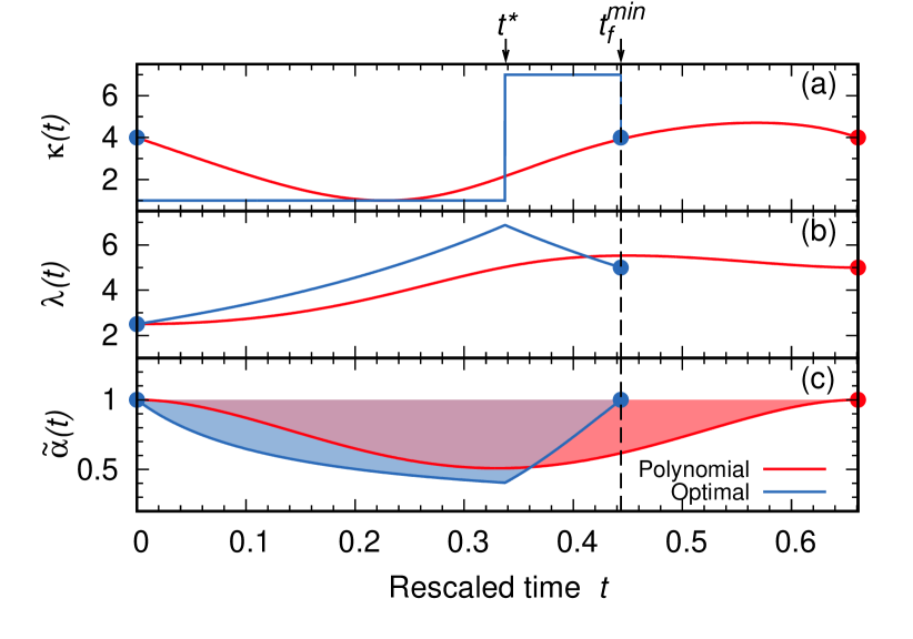
Figure 2: Evolution of the parameters for the minimum-time protocol and for the solution to Eqs. (6) associated to the polynomial with coefficients (10). Panel (a) shows the time dependence of $\kappa(t)$, panel (b) that of $\lambda(t)$ and panel (c) the evolution of $\widetilde{\alpha}(t)$. The dashed vertical line identifies the minimum time over all possible protocols of the type given by Eq. (4), with $1<\kappa<7$. The switching time $t^{\star}$ is also highlighted on the top axis. The shaded areas in panel (c) do not depend on the protocol, once the r.h.s. of Eq. (12) is fixed (here $\kappa_{0}=4$, $\lambda_{i}=2.5$ and $\lambda_{f}=5$).

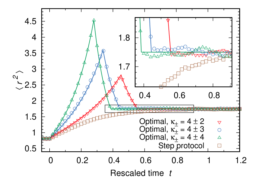
Figure 3: Comparison between the relaxation dynamics induced by a step-protocol and the optimal control protocol. In the former case (brown squares), the value of $\lambda$ is suddenly changed from $\lambda_{i}$ to $\lambda_{f}$ at $t=0$; in the latter the optimal protocol described in the text is operated, for different values of the bounds $\kappa_{\pm}$. Symbols refer to the instantaneous value of $\left\langle r^{2}\right\rangle$, computed as an average over $10^{4}$ independent numerical simulations (see SM SM for details). Solid lines provide the analytical prediction (only for the controlled protocols). The inset is a zoom on the area enclosed by the rectangle.

Here we have assumed that the stiffness of the confining potential can be varied discontinuously. In the SM SM we show that this limit protocol can be approached with arbitrary precision by continuous-in-time protocols.

The minimal time $t_{f}^{min}$ should not be interpreted as a definitive bound, as it has been derived by only considering solutions of the form (4) with constant $\widetilde{\kappa}=\kappa_{0}$: even faster protocols might be achievable, in principle, by allowing for more general functional forms of our ansatz.

Conclusions — In the present letter, we have discussed a class of exact analytical protocols to bring an ABP system from an initial non-equilibrium stationary state to another final stationary state having a different degree of activity, in a given time. Among this family of protocols, we have also identified the one leading to the minimal time. The proposed protocols are expected to be relevant in actual experiments with tunable active particles,

The present work extends the quest for controlling stochastic motion to the realm of active particles. To the best of our knowledge, this is the first case in which SST can be found for this class of systems, and one of the few involving out-of-equilibrium models Baldassarri et al. (2020); Prados (2021); Baldovin et al. (2022).

Our computation is the starting point for the solution of other optimal problems for ABPs: for instance, the average work done during a realization can be computed SM and minimized with analytical methods, a task that has been so far accomplished, for active models, only with numerical techniques Nemoto et al. (2019). Since our search for the optimal protocol is restricted to the class of processes fulfilling condition (4), a further step would consist in proving (or excluding) that the “global” optimum belongs to this family, making use of Pontryagin’s principle Pontryagin (1987). Protocols connecting states with different stiffness may be also searched for, following similar approaches. Future developments pertain to the search for SSTs in three dimensions Turci and Wilding (2021) (e.g., in the presence of homogeneous external force Vachier and Mazza (2019)), and for interacting particles Pototsky and Stark (2012); Solon et al. (2015b); the latter has been studied in the context of passive systems Dago et al. (2020), but with few degrees of freedom only.

Similar strategies may be attempted for active particle models whose stationary state is analytically known, as the 1D Run-and-Tumble Tailleur and Cates (2009); Dhar et al. (2019) or the Active Ornstein-Uhlenbeck particles with Unified Color Noise approximation Maggi et al. (2015b); Caprini et al. (2019). We emphasize that our method, based on suitable deformations of the stationary distribution, may be used to search for SST in different contexts, provided that the stationary state is known. Finding the general conditions to be fulfilled for this approach to provide a suitable solution is an interesting research perspective.