Boosting Semi-Supervised Learning with Contrastive Complementary Labeling

Abstract

Semi-supervised learning (SSL) has achieved great success in leveraging a large amount of unlabeled data to learn a promising classifier. A popular approach is pseudo-labeling that generates pseudo labels only for those unlabeled data with high-confidence predictions. As for the low-confidence ones, existing methods often simply discard them because these unreliable pseudo labels may mislead the model. Nevertheless, we highlight that these data with low-confidence pseudo labels can be still beneficial to the training process. Specifically, although the class with the highest probability in the prediction is unreliable, we can assume that this sample is very unlikely to belong to the classes with the lowest probabilities. In this way, these data can be also very informative if we can effectively exploit these complementary labels, i.e., the classes that a sample does not belong to. Inspired by this, we propose a novel Contrastive Complementary Labeling (CCL) method that constructs a large number of reliable negative pairs based on the complementary labels and adopts contrastive learning to make use of all the unlabeled data. Extensive experiments demonstrate that CCL significantly improves the performance on top of existing methods. More critically, our CCL is particularly effective under the label-scarce settings. For example, we yield an improvement of 2.43% over FixMatch on CIFAR-10 only with 40 labeled data.

1 Introduction

Deep networks have been the workhorse of many computer vision tasks, including image classification [33, 29, 64, 26, 23, 13, 28, 12], semantic segmentation [52, 48], and many other areas [69, 19, 57, 22, 24, 20, 5, 51]. Recently, semi-supervised learning (SSL) has achieved great success in training deep models on large-scale datasets without expensive labeling costs [65, 75, 71, 16]. Compared to the standard supervised learning scheme, SSL can unleash the power of large amounts of unlabeled data to learn better classifiers, which is especially effective under a labels-scarce setting. One technique that is widely used in SSL methods is pseudo-labeling, which generates pseudo labels for unlabeled data to provide additional supervision information. In practice, the quality of pseudo labels is critical to the performance of SSL methods. To avoid low-quality pseudo labels hindering training, a common strategy is to generate pseudo labels only for unlabeled data with high-confidence predictions, while discarding other unlabeled data entirely.

However, this simple selective strategy leads to limited utilization of unlabeled data, as these discarded unlabeled data may contain information that can be further exploited. Some advanced methods  [46, 71, 41] try to use contrastive learning to further mine the information in low-confidence unlabeled data, to effectively use unlabeled data. One representative work, CCSSL [71], directly uses low-confidence unlabeled data to construct pairs and further computes supervised contrastive loss [40]. As a result, CCSSL improves SSL methods by mining extra information for low-confidence unlabeled data to a certain extent, but still inevitably leads to suboptimal models. Since CCSSL may mistakenly push data belonging to the same class away based on the low-confidence pseudo labels, the discriminative power of the model will be weakened.

To address the issue, we hope to reduce possible noises when using low-confidence unlabeled data for training. Intuitively, we should keep data that may belong to the same class close to each other in the feature space. However, unlabeled data with low-confidence often produce a very noisy signal about which classes they should belong to, i.e., the classes with the highest probability in predictions are considered unreliable. On the contrary, we can always confidently keep the data with low-confidence away from the region of the class with the lowest probability. For each low-confidence data, the class it is most unlikely to belong to is considered as its complementary label. From this point of view, if we can better make use of these complementary labels, the low-confidence unlabeled data can help to learn a discriminative SSL model.

Inspired by this, we seek to leverage the complementary labels of data with low-confidence. Nevertheless, these complementary labels cannot be directly used to compute the cross-entropy loss. Instead, we propose a Contrastive Complementary Labeling (CCL) method which constructs reliable negative pairs for low-confidence data based on their complementary labels and further performs contrastive learning. Specifically, we construct reliable negative pairs between either two high-confidence samples or one high-confidence sample together with a low-confidence sample. We highlight that these pairs are reliable because both the labels of high-confidence samples (the former case) and the complementary labels of low-confidence samples (the latter case) are considered reliable. But unlike standard complementary labels that only take the class with the lowest probability, we select several low-probability classes as complementary labels for low-confidence unlabeled data. This pair construction strategy enables CCL to construct a large number of reliable negative pairs, which are beneficial for the subsequent contrastive learning. As for positive pairs, we only consider the samples that belong to the same class or are generated through different augmentations from the same image. In this way, both the negative pairs and positive pairs become reliable. More critically, unlike most existing methods that directly discard those low-confidence samples, we highlight that our CCL method takes all the unlabeled data into account. Extensive experiments show that CCL can be easily integrated with existing advanced SSL methods and significantly outperform the baselines under the label-scarce settings.

Our contributions can be summarized as follows:

• We propose a novel Contrastive Complementary Labeling (CCL) method that constructs reliable negative pairs based on the complementary labels, i.e., the classes that a sample does not belong to. Indeed, our CCL effectively exploits low-confidence samples to provide additional information for the training process.

• We develop a complementary labeling strategy to construct reliable negative pairs. Specifically, for low-confidence data, we first select multiple classes with the lowest probability as complementary labels. Then reliable complementary labels are applied to construct a large number of negative pairs, which greatly benefits the contrastive learning.

• Extensive experiments on multiple benchmark datasets show that CCL can be easily integrated with existing advanced pseudo-label-based end-to-end SSL methods (e.g., FixMatch) and finally yield better performance. Besides, under the label-scarce settings, CCL effectively unleashes the power of data with low-confidence, thus achieving a significant improvement of 2.43%, 6.35%, and 1.78% on CIFAR-10, STL-10, and SVHN only with 40 labeled data, respectively.

Figure 1: The schema of the proposed Contrastive Complementary Labeling (CCL) method. Given a batch of labeled data $\mathcal{X}$ and unlabeled data $\mathcal{U}$, the input data $x_{i}$ will go through the classifier to generate pseudo labels $\hat{y}_{i}$ and obtain complementary labels via $\Phi(x_{i})$. Then we divide the input data with their pseudo labels into the high-confidence set $\mathbb{H}$ and the low-confidence set $\mathbb{L}$. The projector head helps map features to the normalized embeddings to compute the contrastive loss $\mathcal{L}_{c}$. By constructing positive pairs and negative pairs with complementary labels, we focus on leveraging reliable information from those low-confidence unlabeled data.

2 Related Work

2.1 Semi-Supervised Learning

Semi-supervised learning (SSL) mainly include consistency regularization method and pseudo-labeling methods, which aims at taking advantage of unlabeled data to improve performance. Specifically, consistency regularization methods [38, 63, 44, 67, 68, 49, 39, 81, 47, 61, 21, 2, 76, 43, 25, 50, 27, 18, 58, 6, 31] construct different views from the same image, based on the assumption that perturbation of images can not cause significant change of the classifier output. Pseudo-labeling methods [55, 62, 79, 78, 80, 66, 70] rely heavily on confidence threshold, where choosing the appropriate threshold is important to achieving high performance.

Recently, ReMixMatch [3] uses weak augmentation to create pseudo labels and enforce consistency against strong augmentation samples. FixMatch [65] and UDA [68] rely on a fixed threshold during training, and only retain the unlabeled data whose prediction probability is above the threshold. Based on the limitations of the threshold setting of FixMatch, FlexMatch [75] proposes Curriculum Pseudo Labeling to adjust thresholds flexibly for different classes, which effectively leverages unlabeled data. With the help of contrastive learning in SSL, CoMatch [46] and CCSSL [71] cluster samples with similar pseudo labels to alleviate the problem that the model cannot mine information from unreliable low-confidence unlabeled data. Inspire by these works, CCL further uses multiple complementary labels to construct reliable negative pairs, and then provides additional discriminative information for contrastive learning, thereby facilitating the utilization of unlabeled data.

2.2 Contrastive Learning

Contrastive learning methods have been fully developed in recent years. [34, 35, 30] propose and refine Noise Contrastive Estimation (NCE). [59] proposes InfoNCE to help the model capture valuable information for future prediction. In self-supervised learning, contrastive learning is widely applied and has shown strong performance [8, 9, 32, 17, 10, 74, 11, 7]. Self-supervised contrastive learning constructs a latent feature space for the downstream task. To leverage label information effectively, SupCon [40] clusters the same class samples and pulls apart different classes. Combining SupCon, full-supervised learning obtains a significant improvement in image classification.

Recently, some methods have been successfully applied in different domains by combining contrastive learning. For example, [1] proposes a pixel-level contrastive learning scheme for SSL semantic segmentation with a memory bank for pixel-level features from labeled data. [60] improves fine-tuning of self-supervised pretrained models with contrastive learning. In the SSL classification task, [77] and [41] combine self-supervised contrastive learning with cross-entropy and consistency regularization to achieve better performance, respectively. Our method differs from them by constructing reliable negative pairs based on complementary labels in a novel strategy, which is beneficial for subsequent contrastive learning.

2.3 Complementary Labeling

Complementary labels indicate which classes the image does not belong to. Compared with ordinary labels, complementary labels are sometimes easily obtainable, especially when the class set is relatively large. For classification with complementary labels, [36] provides an unbiased estimation for the expected risk of classification with true labels and proposes a framework to minimize it. [37] modifies the theories and frameworks in [36] and improves its performance. [72] further addresses the problem of learning with biased complementary labels. It is worth mentioning that [36, 37] only consider using a single class with the lowest probability as a complementary label. Different from them, CCL considers multiple unlikely classes as complementary labels for each low-confidence data to provide more discriminative information.

However, complementary labels can not be directly used to compute cross-entropy. MutexMatch [16] proposes to train a distinct classifier TNC for predicting complementary labels, thus helping to learn the representation of unlabeled data from a mutex perspective and greatly boosting SSL methods. Instead of incorporating complementary labels into computing cross-entropy loss, CCL naturally constructs reliable negative pairs based on complementary labels and further computes the contrastive loss.

3 Proposed Method

In this paper, we seek to improve SSL by leveraging reliable information from those low-confidence unlabeled data. To this end, we propose a Contrastive Complementary Labeling (CCL) method that generates a large number of reliable negative pairs based on the classes that a sample does not belong to, namely complementary labels. For clarity, in Section 3.1, we first discuss some important notations and preliminaries. Then, in Section 3.2, we develop the rules on how to construct reliable negative pairs and incorporate them into the contrastive learning scheme. The overview of the proposed CCL method is shown in Figure 1.

3.1 Notations and Preliminaries

We consider the semi-supervised setting where the training data consists of some labeled data along with a large number of unlabeled data. Let $\mathcal{X}{=}\left\{\left(x_{i},y_{i}\right)\right\}_{i=1}^{B}$ be a batch of $B$ labeled samples where $x_{i}$ and $y_{i}$ are the training sample and the corresponding label, respectively. Let $\mathcal{U}{=}\left\{u_{i}\right\}_{i=1}^{\mu B}$ be a batch of $\mu B$ unlabeled samples where $\mu$ denotes the relative sizes of $\mathcal{X}$ and $\mathcal{U}$. Following [65], we use the weak augmentation $\alpha(\cdot)$ to transform all the training data and additionally use a strong augmentation $\mathcal{A}(\cdot)$ to produce an extra view of the unlabeled data. In total, we consider three kinds of data, i.e., $\alpha(\mathcal{X})$, $\alpha(\mathcal{U})$, and $\mathcal{A}(\mathcal{U})$.

In this paper, we consider a deep network that consists of an encoder, a classifier head, and a projector head. The encoder extracts features of images and the classifier further produces the predicted logits. We use a projector head to map features to the normalized embeddings to compute the contrastive loss. When generating pseudo labels, we first obtain the prediction $f(\cdot)$ of the weakly augmented view and enforce the corresponding strongly augmented view to share the same logits and pseudo label. To achieve this, we define a function $\psi(x)$ that returns the weakly augmented view of any given data $x$. Formally, the predictions of different data can be formulated by:

$$\hat{p}_{i}=\left\{\begin{array}[]{*{35}{l}}f(x_{i})&\text{if }{{x}_{i}}\in\alpha(\mathcal{X}),\\ f(\psi(x_{i}))&\text{otherwise}.\\ \end{array}\right.$$ (1)

Based on Eq. 1, we further compute the (pseudo) label for each sample. For labeled data, we directly take the ground-truth labels $y_{i}$. For unlabeled data, we focus on the largest item of $\hat{p}_{i}$ and use a confidence threshold $\tau$ to select those high-confidence samples with $\max({{\hat{p}}_{i}})\geq\tau$. In practice, we leave the other low-confidence samples with $\hat{y}_{i}=-1$ since their pseudo labels are often unreliable. In summary, the labels $\hat{y}_{i}$ of different data becomes:

$$\hat{y}_{i}=\left\{\begin{array}[]{*{35}{l}}y_{i}&\text{if }{{x}_{i}}\in\alpha({\mathcal{X}}),\\ \operatorname*{arg\,max}(\hat{p}_{i})&\text{else if}~{}\max({{\hat{p}}_{i}})\geq\tau,\\ -1&\text{otherwise}.\\ \end{array}\right.$$ (2)

In summary, all the labeled data and unlabeled data, along with their labels, can be written as $\mathbb{Q}=\left\{\left(x_{i},\hat{y}_{i}\right)\right\}_{i=1}^{(2\mu+1)B}$, where $x_{i}\in\alpha(\mathcal{X})\cup\alpha(\mathcal{U})\cup\mathcal{A}(\mathcal{U})$. Based on the above definitions, we take both labeled data and the high-confidence unlabeled data as the high-confidence set:

$$\mathbb{H}=\{\left(x_{i},\hat{y}_{i}\right)|x_{i}\in\alpha(\mathcal{X}){~{}\rm or~{}}\max({{\hat{p}}_{i}})\geq\tau\}.$$ (3)

And leave the rest as the low-confidence set $\mathbb{L}=\mathbb{Q}\setminus\mathbb{H}$. In practice, most SSL methods simply discard the use of noisy $\mathbb{L}$, however, these low-confidence data may still provide some useful information.

3.2 Contrastive Complementary Labeling

Besides the samples in high-confidence set $\mathbb{H}$, we seek to further exploit those low-confidence samples in $\mathbb{L}$ to aid the training. Although taking the class with the largest probability as the label is very noisy for the low-confidence samples, those classes with particularly low probabilities should still be relatively reliable to indicate which classes a sample does not belong to. For clarity, we refer to these unlikely classes as complementary labels in this paper.

Although these complementary labels become potentially informative, it is non-trivial to directly use them to compute the cross-entropy loss. Instead, we can easily construct negative pairs between a low-confidence sample and a large number of high-confidence samples in $\mathbb{H}$ that belong to classes in the complementary label of the low-confidence sample. Interestingly, these negative pairs can be naturally incorporated into the contrastive learning scheme [40]. Inspired by this, we propose a Contrastive Complementary Labeling (CCL) method that constructs reliable negative pairs based on the complementary labels. The detailed training method is shown in Algorithm 1. In the following, we will discuss the construction of complementary labels and the specific strategy to construct reliable negative and positive pairs upon them.

Algorithm 1 Training method of Contrastive Complementary Labeling (CCL). We obtain multiple complementary labels for each sample and build reliable negative pairs based on them to compute the contrastive loss.

Input: Labeled data ${\mathcal{X}}$, unlabeled data ${\mathcal{U}}$, the function to obtain complementary labels for a sample $\Phi(\cdot)$, the function to return the weakly augmented view of a sample $\psi(\cdot)$, the number of classes in complementary labels ${k}$.

1:  // Obtain pseudo labels for unlabeled data

2:  for $x_{i}\in\mathcal{U}$ do

3:     Obtain predicted class distribution $\hat{p}_{i}$ via Eq. 1

4:     Compute the pseudo label $\hat{y}_{i}$ using Eq. 2

5:  end for

6:  // Construct negative pairs and positive pairs

7:  Divide $\mathbb{Q}$ into the high-confidence set $\mathbb{H}$ and the low-confidence set $\mathbb{L}$ via Eq. 3

8:  Obtain complementary labels via $\Phi(x_{i})=\left\{\begin{array}[]{*{35}{l}}\{c\in\mathcal{O}_{i}|c\neq\hat{y}_{i}\}&\text{if }{{x}_{i}}\in\mathbb{H},\\ \{c\in\mathcal{O}_{i}|\mathcal{O}_{i}(c)<k\}&\text{otherwise}.\\ \end{array}\right.$

9:  Construct negative pairs using $\mathbb{N}({{x}_{i}})=\{{{x}_{j}}\in\mathbb{Q}|{\hat{y}_{j}}\in{\Phi(x_{i})}{~{}\rm or~{}}\hat{y}_{i}\in{\Phi(x_{j})}\}$.

10:  Construct positive pairs using $\mathbb{P}(x_{i}){=}\left\{\begin{array}[]{*{35}{l}}\{{{x}_{j}}\in\mathbb{Q}{\setminus}\{x_{i}\}|{\hat{y}_{i}}{=}{\hat{y}_{j}}\}&\text{if}\text{ }x_{i}\in\mathbb{H},\\ \{{{x}_{j}}\in\mathbb{Q}{\setminus}\{x_{i}\}|\psi(x_{i}){=}\psi(x_{j})\}&\text{otherwise}.\\ \end{array}\right.$

11:  Compute contrastive loss $\mathcal{L}_{c}$ via Eq. 7

12:  Compute total loss $\mathcal{L}=\mathcal{L}_{x}+\mathcal{L}_{u}+\mathcal{L}_{c}$ to update model

Constructing negative pairs with complementary labels.

For any sample $x_{i}\in\mathbb{Q}$, we seek to construct the complementary labels based on its predicted class distribution $\hat{p}_{i}$. Since we seek to identify the complementary classes that a sample does not belong to, we sort $\hat{p}_{i}$ in the ascending order and obtain the indices of classes via ${{\mathcal{O}}_{i}=\operatorname*{arg\,sort}(\hat{p}_{i})}$. Actually, the standard complementary labeling [36] only selects the first one, i.e., the class with the lowest probability, as the complementary label. Nevertheless, given a number of classes in total, e.g., $C{=}10$ for CIFAR-10, the second or even the first five items in $\mathcal{O}$ may also have very low probabilities and can be potentially used to construct the complementary labels. Inspired by this, we propose a flexible complementary labeling strategy that selects multiple unlikely classes as complementary labels for each low-confidence sample. As for the high-confidence sample $x\in\mathbb{H}$, we directly take all the classes other than its ground-truth label as the complementary labels. For convenience, we use ${\mathcal{O}}_{i}(c)$ to denote the position of class $c$ in $\mathcal{O}_{i}$. Formally, the complementary label of $x_{i}$ can be written by:

$$\Phi(x_{i})=\left\{\begin{array}[]{*{35}{l}}\{c\in\mathcal{O}_{i}|c\neq\hat{y}_{i}\}&\text{if }{{x}_{i}}\in\mathbb{H},\\ \{c\in\mathcal{O}_{i}|\mathcal{O}_{i}(c)<k\}&\text{otherwise},\\ \end{array}\right.$$ (4)

where $k$ denotes the number of unlikely classes selected as complementary labels (see ablations on $k$ in Figure 5).

Based on the complementary labels, we further discuss how to construct reliable negative pairs. As shown in Figure 2(a), we construct reliable negative pairs between either two high-confidence samples (i.e., left top corner) or one high-confidence together with a low-confidence sample (i.e., left bottom and right top corner). In the former case, for any two samples $x_{i},x_{j}\in\mathbb{H}$, they become a negative pair as long as one of them belongs to the complementary label of another, i.e., ${\hat{y}_{j}}\in{\Phi(x_{i})}{~{}\rm or~{}}\hat{y}_{i}\in{\Phi(x_{j})}$. As for the latter case, for any low-confidence sample $x\in\mathbb{L}$, we select all the samples in $\mathbb{H}$ that belong to its complementary label set $\Phi(x)$ to construct negative pairs. We highlight that these pairs are reliable because both the labels of high-confidence samples and the complementary labels of the considered low-confidence sample are reliable. Since the data usage matrix in Figure 2(a) is symmetric, we can always construct a negative pair as long as one sample belongs to the complementary labels of another one, which shares the same rule as the case for two high-confidence samples. Formally, the set of negative pairs for any sample $x\in\mathbb{Q}$ becomes:

$$\mathbb{N}({{x}_{i}})=\{{{x}_{j}}\in\mathbb{Q}|{\hat{y}_{j}}\in{\Phi(x_{i})}{~{}\rm or~{}}\hat{y}_{i}\in{\Phi(x_{j})}\}.$$ (5)

As mentioned above, for any low-confidence sample, we can always go through the whole high-confidence set $\mathbb{H}$ to construct negative pairs. In this sense, the proposed CCL method is able to construct a large number of reliable negative pairs and thus provide richer information for contrastive learning. From this point of view, we highlight that the improvement achieved by our CCL mainly stems from a large amount of reliable negative pairs.

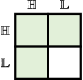
(a) The data used to construct negative pairs in the proposed CCL.

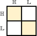
(b) The data used to construct positive pairs in the proposed CCL.

Figure 2: The data usage matrix for constructing pairs. The shaded regions in (a) represent three cases of constructing negative pairs by Eq. 5, and the shaded regions in (b) represent two cases of constructing positive sample pairs by Eq. 6. Adopting this data usage strategy can make better use of low-confidence data.

Constructing positive pairs.

Inspired by [40] and [59], we only construct positive pairs for two reliable cases to reduce possible noise from the unreliable predictions of unlabeled data as shown in Figure 2(b). First, under the guidance of $\hat{y}$, any two samples $x_{i},x_{j}\in\mathbb{H}$ from the same class, i.e., $\hat{y}_{i}=\hat{y}_{j}$, are considered as a positive pair and should be pulled closer to each other. Second, for the low-confidence set $\mathbb{L}$, we construct positive pairs for samples $x_{i}$ and $x_{j}$ only when they are two augmented views of the same image. Since we use $\psi(\cdot)$ to retrieve the weakly augmented view of an image, the above condition can be equivalently cast into sharing the same weakly augmented view, i.e., $\psi(x_{i})=\psi(x_{j})$. For all the other cases with one high-confidence sample and one low-confidence sample (blank regions in Figure 2(b)), we do not construct any positive pairs since they are always unreliable, i.e., $\hat{y}=-1$. Formally, the set of positive pairs for any sample $x\in\mathbb{Q}$ is:

$$\mathbb{P}(x_{i})=\left\{\begin{array}[]{*{35}{l}}\{{{x}_{j}}\in\mathbb{Q}\setminus\{x_{i}\}|{\hat{y}_{i}}={\hat{y}_{j}}\}&\text{if}\text{ }x_{i}\in\mathbb{H},\\ \{{{x}_{j}}\in\mathbb{Q}\setminus\{x_{i}\}|\psi(x_{i})=\psi(x_{j})\}&\text{otherwise}.\\ \end{array}\right.$$ (6)

Method	CIFAR-10			STL-10			SVHN
	40	250	4000	40	250	1000	40	1000
Fully-Supervised	95.38$\pm$0.05			None			97.87$\pm$0.01
$\pi$ - Model [63]	25.66$\pm$1.76	53.76$\pm$1.29	86.87$\pm$0.59	25.69$\pm$0.85	44.87$\pm$1.50	67.22$\pm$0.40	32.52$\pm$0.95	92.84$\pm$0.11
Pseudo-Label [45]	25.39$\pm$0.26	53.51$\pm$2.20	84.92$\pm$0.19	25.32$\pm$0.99	44.55$\pm$2.43	67.36$\pm$0.71	35.39$\pm$5.60	90.60$\pm$0.32
Mean Teacher [67]	29.91$\pm$1.60	62.54$\pm$3.30	91.90$\pm$0.21	28.28$\pm$1.45	43.51$\pm$2.75	66.10$\pm$1.37	63.91$\pm$3.98	96.73$\pm$0.05
VAT [54]	25.34$\pm$2.12	58.97$\pm$1.79	89.49$\pm$0.12	25.26$\pm$0.38	43.58$\pm$1.97	62.05$\pm$1.12	25.25$\pm$3.38	95.89$\pm$0.20
MixMatch [4]	63.81$\pm$6.48	86.37$\pm$0.59	93.34$\pm$0.26	45.07$\pm$0.96	65.48$\pm$0.32	78.30$\pm$0.68	69.40$\pm$8.39	96.31$\pm$0.37
ReMixMatch [3]	90.12$\pm$1.03	93.70$\pm$0.05	95.16$\pm$0.01	67.88$\pm$6.24	87.51$\pm$1.28	93.26$\pm$0.14	75.96$\pm$9.13	94.84$\pm$0.31
UDA [68]	89.38$\pm$3.75	94.84$\pm$0.06	95.71$\pm$0.07	62.58$\pm$8.44	90.28$\pm$1.15	93.36$\pm$0.17	94.88$\pm$4.27	98.11$\pm$0.01
MutexMatch [16]	93.22$\pm$2.52	-	-	-	-	-	97.19$\pm$0.26	-
CCSSL [71]	90.83$\pm$2.78	94.86$\pm$0.55	95.54$\pm$0.20	-	-	-	-	-	-
FixMatch [65]	92.53$\pm$0.28	95.14$\pm$0.05	95.79$\pm$0.08	64.03$\pm$4.14	90.19$\pm$1.04	93.75$\pm$0.33	96.19$\pm$1.18	98.04$\pm$0.03
CCL-FixMatch (ours)	94.96$\pm$0.11${}_{{\color[rgb]{0,0,1}\mbox{\scriptsize+2.43}}}$	95.15$\pm$0.04${}_{{\color[rgb]{0,0,1}\mbox{\scriptsize+0.01}}}$	95.80$\pm$0.05${}_{{\color[rgb]{0,0,1}\mbox{\scriptsize+0.01}}}$	70.38$\pm$3.41${}_{{\color[rgb]{0,0,1}\mbox{\scriptsize+6.35}}}$	91.23$\pm$0.44${}_{{\color[rgb]{0,0,1}\mbox{\scriptsize+1.04}}}$	94.10$\pm$0.27${}_{{\color[rgb]{0,0,1}\mbox{\scriptsize+0.35}}}$	97.97$\pm$0.45${}_{{\color[rgb]{0,0,1}\mbox{\scriptsize+1.78}}}$	98.13$\pm$0.03${}_{{\color[rgb]{0,0,1}\mbox{\scriptsize+0.09}}}$

Table 1: Top-1 accuracy on CIFAR-10, STL-10, and SVHN datasets. STL-10 dataset does not have label information for unlabeled data, so it does not have fully-supervised results. The bold number indicates the best result. The blue values show the improved accuracy of our CCL-FixMatch over FixMatch. We achieve the best performance by simply adding CCL to Fixmatch.

Training objective.

In the training schema of CCL, we first obtain the pseudo labels and complementary labels for each unlabeled data. Then, we construct reliable negative pairs and positive pairs based on complementary labels. Finally, by optimizing the contrastive loss, the discriminative ability of the model is improved. The contrastive loss $\mathcal{L}_{c}$ takes the following format:

$$\begin{split}\mathcal{L}_{c}{=}-\sum_{{{x}_{i}}\in\mathbb{Q}}{\frac{1}{|\mathbb{P}({{x}_{i}})|}\sum\limits_{{{x}_{j}}\in\mathbb{P}({{x}_{i}})}{\log\frac{{e}\frac{z({{x}_{i}})\cdot z({{x}_{j}})}{T}}{\sum\limits_{{{x}_{k}}\in\mathbb{P}({{x}_{i}})\cup\mathbb{N}({{x}_{i}})}{{{e}\frac{z({{x}_{i}})\cdot z({{x}_{k}})}{T}}}}}},\end{split}$$ (7)

where $|\mathbb{P}({{x}_{i}})|$ is the cardinality of the positive pairs set. $z(x_{i})$ denotes the feature embedding of $x_{i}$. $T$ is the temperature coefficient and is set to 0.07 by default. Besides $\mathcal{L}_{c}$, we follow [65, 75] and consider two additional loss terms to build the overall training objective. Let $H(\cdot)$ denote the cross-entropy function. We additionally consider a cross-entropy loss on labeled data ${\mathcal{L}}_{x}{=}\frac{1}{B}\sum_{i=1}^{B}{H\left(y_{i},\hat{p}_{i}\right)}$ and a loss on unlabeled data ${{\mathcal{L}}_{u}}{=}\frac{1}{\mu B}\sum_{i=1}^{\mu B}{\mathbbm{1}}\left(\max(\hat{p}_{i})\geq\tau\right)H\left(\hat{y}_{i},f(\mathcal{A}(u_{i}))\right)$. Thus, the overall loss of our CCL can be written as:

$$\mathcal{L}=\mathcal{L}_{x}+\mathcal{L}_{u}+\mathcal{L}_{c}.$$ (8)

4 Experiments

In this section, we evaluate the effectiveness of CCL on various SSL datasets. We first describe the main experimental datasets and the training settings in Section 4.1. We then compare CCL with other advanced methods in Section 4.2. Finally, we present detailed analyses to help understand the advantages of CCL in Section 4.3. Code and pretrained models for our CCL will be available soon.

4.1 Datasets and Training Settings

Following [65, 71, 75, 46], we conduct extensive experiments on several benchmarks, including CIFAR-10 [42], STL-10 [14], SVHN [56], and CIFAR-100 [42], each with various amounts of labeled data. Due to page limitation, we put the results on CIFAR-100 in the supplementary.

Datasets.

We conduct experiments on CIFAR-10 with 40, 250, and 4000 labeled data, STL-10 with 40, 250, and 1000 labeled data, and SVHN with 40 and 1000 labeled data. CIFAR-10 [42] are all known classes, and the data distribution in each class is balanced. CIFAR-10 contains 50,000 training images and 10,000 test images and each of the colored images is 32$\times$32 pixels in 10 classes. STL-10 [14] contains 5000 labeled images and 100,000 unlabeled images. All images are in color and are 96x96 pixels in size. However, the unlabeled images are extracted from a similar but broader distribution of images, which contain unknown classes. SVHN [56] is a relatively simple (i.e., to classify digits) yet unbalanced dataset with 10 classes, which contains a training set, a test set, and 531,131 additional images in the extra set. Note that our experiment also includes the extra set. These unlabeled images of SVHN with unbalanced distribution will bring more challenges to the SSL.

Training settings.

For a fair comparison, we use the same hyper-parameters following the common codebase TorchSSL [75]. We use Wide ResNet-28-2 [73] for CIFAR-10, STL-10, and SVHN. In the testing phase, we perform all algorithms using an exponential moving average with the momentum of $0.999$. In a mini-batch, 64 labeled data and $\mu\times 64$ unlabeled data are randomly sampled, where the unlabeled data ratio $\mu$ is set to $7$. The optimizer for all experiments is standard stochastic gradient descent (SGD) with the momentum of $0.9$. For all datasets, we use cosine learning rate decay schedule [53] as $\eta=\eta_{0}\cos\left(\frac{7\pi t}{16N}\right)$, where $\eta_{0}=0.03$ is the initial learning rate, $t$ is the current training step, and $N$ is the total training step that is set to $N=2^{20}$ for all datasets. The default confidence threshold $\tau$ is set to 0.95. The default number of classes in complementary labels $k$ is set to 7. In all of our experiments, the weak augmentation $\mathcal{\alpha}(\cdot)$ is a random flip-and-shift augmentation strategy, and the strong augmentation $\mathcal{A}(\cdot)$ is RandAugment [15]. Following [75], we run each task three times using random seed 0, 1, 2 for all experiments and report the best top-1 accuracy of all checkpoints. Detailed hyper-parameters are introduced in the supplementary.

4.2 Comparisons on Standard Benchmarks

We compare our method with some advanced SSL methods, including $\pi$ - Model [63], Pseudo-Label [45], Mean Teacher [67], VAT [54], MixMatch [4], ReMixMatch [3], UDA [68], MutexMatch [16], CCSSL [71] and FixMatch [65]. Meanwhile, we also report the results of full-supervised learning with all data labeled on CIFAR-10 [42] and SVHN [56]. What’s more, we also provide the detailed precision, recall, F1, and AUC results in the supplementary.

Constructing Pairs in $\mathbb{H}$	Constructing Pairs in $\mathbb{L}$	Constructing Pairs with Complementary Labels Based on Equation 5 and Equation 6	CIFAR-10 w/ 40
$\times$	$\times$	$\times$	92.53 (baseline)
✓	$\times$	$\times$	93.68${}_{{\color[rgb]{0,0,1}\mbox{\scriptsize+1.15}}}$
✓	✓	$\times$	93.03${}_{{\color[rgb]{0,0,1}\mbox{\scriptsize+0.50}}}$
✓	✓	✓	94.96${}_{{\color[rgb]{0,0,1}\mbox{\scriptsize+2.43}}}$

Table 2: Comparison of using different strategies for constructing pairs in contrastive learning on CIFAR-10 with 40 labeled data. The blue values show the improved accuracy of our CCL-FixMatch over FixMatch (baseline). Results show that the strategy of using complementary labels to construct reliable negative pairs for contrastive learning can significantly improve model performance.

In Table 1, we find that CCL is helpful for FixMatch for all benchmarks and CCL achieves better performance when the task contains more noise (i.e., fewer labels). For example, under the setting of CIFAR-10 with only 4 labeled data per class, CCL achieves $+2.43\%$ on FixMatch. On unbalanced dataset SVHN, CCL-FixMatch also improves $1.78$% and $0.09$% performance over FixMatch for 40 and 1000 labels. STL-10 dataset is a more complicated and more realistic task since the existence of unknown classes in the unlabeled data. However, in such a challenging case, CCL-FixMatch achieves $+6.35$%, $+1.04$% and $+0.35$% accuracy improvement on FixMatch of STL-10 with 40, 250 and 1000 labeled data, respectively. The decrease in performance gain can be explained as the increasing discriminative ability of the model with the help of more labeled training data. And a well-performing model can also be obtained in less noisy settings without the use of contrastive learning. These improvements also demonstrate the capabilities and potential of CCL for real-world applications.

4.3 Advantages of CCL over Existing Methods

Faster convergence with CCL.

In Figure 3, We study the training convergence speed between FixMatch and CCL-FixMatch on CIFAR-10 with 40 labeled data. CCL-FixMatch achieves better performance with fewer training iterations and shows its superior convergence speed. By using contrastive learning with complementary labels, the model can place the positive pairs as close as possible and the negative pairs as far away as possible in the embedding space, which helps to learn a good feature distribution among instances and improves the discriminative ability of the model in the early training stage. Through our reliable pair construction strategy, the model can better utilize the information of unreliable unlabeled data to guide the learning process and get faster convergence. Therefore, with only 300k iterations, CCL-FixMatch has already surpassed the final results of FixMatch.

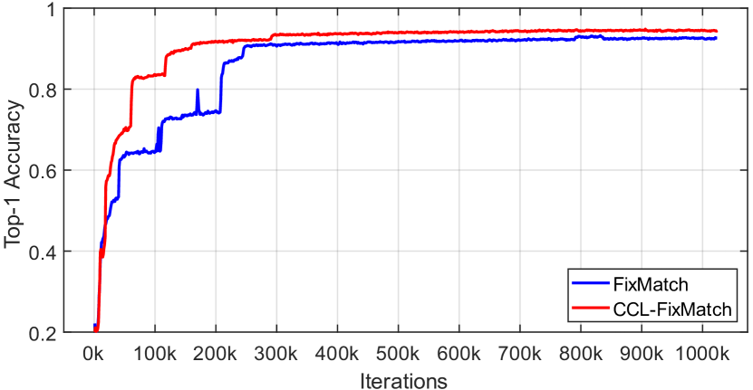
Figure 3: Comparison of the accuracy of FixMatch and CCL-FixMatch on CIFAR-10 with 40 labeled data. CCL achieves better performance and the model is faster in global convergence.

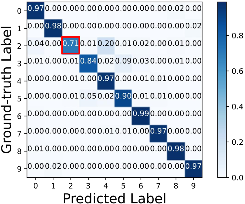
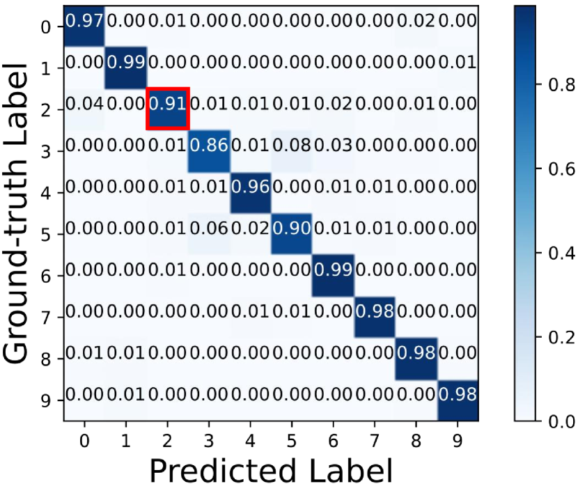
Figure 4: Confusion matrices obtained based on the best checkpoints of FixMatch (left) and CCL-FixMatch (right) on CIFAR-10 with 40 labeled data. The red box indicates the hard class on which FixMatch yields a very low accuracy. By contrast, our CCL model tends to learn a more balanced distribution across different classes.

Superior performance on hard classes.

As shown in Figure 4 (left), the confusion matrix results show that FixMatch is difficult to learn on hard classes. For instance, there are more than 20% examples that belong to class 2 (bird) that are predicted wrongly as class 4 (deer). And CCL obtains a more unbiased confusion matrix as shown in Figure 4 (right). CCL can improve the inter-class separation degree, which promotes the learning of hard classes by the model, improve the quality of pseudo labels, and help to improve the generalization performance.

Method	CIFAR-10			STL-10
	10	20	40	10	20	40
FixMatch [65]	46.47$\pm$20.50	85.81$\pm$7.24	92.53$\pm$0.28	34.43$\pm$2.37	46.89$\pm$2.96	64.03$\pm$4.14
CCL-FixMatch (ours)	49.80$\pm$20.37${}_{{\color[rgb]{0,0,1}\mbox{\scriptsize+3.33}}}$	88.74$\pm$1.27${}_{{\color[rgb]{0,0,1}\mbox{\scriptsize+2.93}}}$	94.96$\pm$0.11${}_{{\color[rgb]{0,0,1}\mbox{\scriptsize+2.43}}}$	40.51$\pm$2.13${}_{{\color[rgb]{0,0,1}\mbox{\scriptsize+6.08}}}$	50.79$\pm$2.09${}_{{\color[rgb]{0,0,1}\mbox{\scriptsize+3.90}}}$	70.38$\pm$3.41${}_{{\color[rgb]{0,0,1}\mbox{\scriptsize+6.35}}}$
FlexMatch [75]	77.85$\pm$17.39	93.20$\pm$2.06	95.03$\pm$0.06	43.99$\pm$3.82	57.63$\pm$1.89	70.85$\pm$4.16
CCL-FlexMatch (ours)	82.88$\pm$16.82${}_{{\color[rgb]{0,0,1}\mbox{\scriptsize+5.03}}}$	94.60$\pm$0.48${}_{{\color[rgb]{0,0,1}\mbox{\scriptsize+1.40}}}$	95.04$\pm$0.06${}_{{\color[rgb]{0,0,1}\mbox{\scriptsize+0.01}}}$	44.39$\pm$3.74${}_{{\color[rgb]{0,0,1}\mbox{\scriptsize+0.40}}}$	57.98$\pm$1.52${}_{{\color[rgb]{0,0,1}\mbox{\scriptsize+0.35}}}$	76.09$\pm$2.05${}_{{\color[rgb]{0,0,1}\mbox{\scriptsize+5.24}}}$

Table 3: Comparison of the performance of different methods on CIFAR-10 and STL-10 only with 10, 20, and 40 labeled data, respectively. The blue values show the improved accuracy of our CCL-FixMatch over FixMatch. CCL-FixMatch/CCL-FlexMatch significantly improves the accuracy and model stability (i.e. smaller standard deviation) of FixMatch/FlexMatch under the label-scare settings.

5 Ablations and Further Discussions

In Section 5.1, We first analyze the influence of different strategies of pairs construction in contrastive learning. Then, in Section 5.2, we further explore the applicability of our method under the label-scare settings. Finally, we investigate the effect of the number of classes to construct complementary labels $k$ in Section 5.3.

5.1 Different Strategies of Pairs Construction

In Table 2, we investigate the effect of contrastive learning with different strategies for pair construction on CIFAR-10 with 40 labeled data. We find that, based on the FixMatch, simply using the pseudo labels of each instance in the high-confidence set $\mathbb{H}$ as supervision information, and introducing supervised contrastive learning [40] to construct positive and negative pairs, can obtain the accuracy of 93.68%, improving the accuracy of FixMatch by 1.15%. However, if we further use the unreliable low-confidence set $\mathbb{L}$ to construct pairs, the performance is improved compared to the baseline but is slightly degraded compared to the strategy of constructing pairs using only $\mathbb{H}$. This suggests that contrastive learning can be effectively applied to SSL when the data is relatively reliable. Therefore, to effectively utilize unlabeled data and reduce noise, we use complementary labels to construct reliable pairs for unreliable low-confidence data, and then use contrastive learning to improve the discriminative ability of the model. With this strategy, the final model improves the performance of SSL and achieves an accuracy of $94.96\%$.

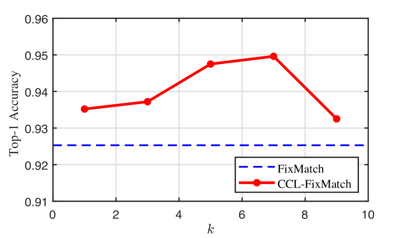
Figure 5: Impact of the number of classes to construct complementary labels, i.e., $k$, on CIFAR-10 with 40 labeled data based on CCL-FixMatch. No matter how we change the value of $k$, we always obtain better results than the baseline model, thanks to the additional information provided by low-confidence samples. In practice, we obtain the best result with $k=7$.

5.2 Comparisons under the Label-Scarce Settings

In Table 3, the results demonstrate that CCL can significantly improve the performance of FixMatch [65] and FlexMatch [75] under the label-scarce setting. CCL-FixMatch consistently outperforms FixMatch under the settings with extremely limited labeled data. For example, on CIFAR-10 with 10, 20, and 40 labeled data, the accuracy is improved by 3.33%, 2.93%, and 2.43%, respectively. On STL-10 with 10, 20, and 40 labeled data, CCL-FixMatch outperforms Fixmatch by 6.08%, 3.90%, and 6.35%, respectively. Compared to FixMatch which uses fixed predefined thresholds, FlexMatch uses flexible class-specific thresholds. And CCL-FlexMatch can further improve the performance of FlexMatch. For example, on CIFAR-10 with 10, 20 and 40 labeled data, the accuracy improves from 77.85% to 82.88%, from 93.20% to 94.60% and from 95.03% to 95.04%, respectively. On STL-10 with 10, 20, and 40 labeled data, CCL-FlexMatch improves the performance by 0.40%, 0.35%, and 5.24% respectively compared to the accuracy of FlexMatch. In brief, CCL can utilize contrastive learning with complementary labels to effectively alleviate the accumulation of possible noises in the training process.

5.3 Effect of $k$ on Model Performance

In Figure 5, we also study different values of the number of classes to construct complementary labels $k$ on CIFAR-10 with 40 labeled data. We find that the best practice value for $k$ is 7 and that too high or too low $k$ can degrade model performance. The reason for this phenomenon is that different values of $k$ affect the number of negative pairs constructed. Specifically, stricter negative pair construction strategies (i.e. smaller $k$) can reduce noise as much as possible, but a lot of unlabeled data information is reduced to guide model training. On the contrary, too loose negative pair construction strategies (i.e. larger $k$) will increase the number of construction of incorrect negative pairs, which will introduce too much noise in contrastive learning.

6 Conclusion

In this paper, we study how to better leverage unreliable low-confidence unlabeled data but reduce possible noises. To address this issue, we propose a Contrastive Complementary Labeling (CCL) method, which constructs reliable negative pairs based on the complementary labels of low-confidence data. In this way, CCL provides discriminative information for subsequent contrastive learning without introducing possible noises. Extensive experimental results on multiple benchmark datasets show that CCL greatly improves the performance of existing advanced methods, especially under the label-scarce settings.

References

- [1] Inigo Alonso, Alberto Sabater, David Ferstl, Luis Montesano, and Ana C Murillo. Semi-supervised semantic segmentation with pixel-level contrastive learning from a class-wise memory bank. In Proceedings of the IEEE/CVF International Conference on Computer Vision, pages 8219–8228, 2021.
- [2] Ben Athiwaratkun, Marc Finzi, Pavel Izmailov, and Andrew Gordon Wilson. There are many consistent explanations of unlabeled data: Why you should average. In International Conference on Learning Representations, 2018.
- [3] David Berthelot, Nicholas Carlini, Ekin D Cubuk, Alex Kurakin, Kihyuk Sohn, Han Zhang, and Colin Raffel. Remixmatch: Semi-supervised learning with distribution alignment and augmentation anchoring. arXiv preprint arXiv:1911.09785, 2019.
- [4] David Berthelot, Nicholas Carlini, Ian Goodfellow, Nicolas Papernot, Avital Oliver, and Colin A Raffel. Mixmatch: A holistic approach to semi-supervised learning. Advances in neural information processing systems, 32, 2019.
- [5] Jiezhang Cao, Yong Guo, Qingyao Wu, Chunhua Shen, Junzhou Huang, and Mingkui Tan. Adversarial learning with local coordinate coding. In International Conference on Machine Learning, pages 707–715. PMLR, 2018.
- [6] Jiezhang Cao, Yong Guo, Qingyao Wu, Chunhua Shen, Junzhou Huang, and Mingkui Tan. Improving generative adversarial networks with local coordinate coding. IEEE Transactions on Pattern Analysis and Machine Intelligence, 44(1):211–227, 2020.
- [7] Mathilde Caron, Hugo Touvron, Ishan Misra, Hervé Jégou, Julien Mairal, Piotr Bojanowski, and Armand Joulin. Emerging properties in self-supervised vision transformers. In Proceedings of the IEEE/CVF International Conference on Computer Vision, pages 9650–9660, 2021.
- [8] Ting Chen, Simon Kornblith, Mohammad Norouzi, and Geoffrey Hinton. A simple framework for contrastive learning of visual representations. In International conference on machine learning, pages 1597–1607. PMLR, 2020.
- [9] Ting Chen, Simon Kornblith, Kevin Swersky, Mohammad Norouzi, and Geoffrey E Hinton. Big self-supervised models are strong semi-supervised learners. Advances in neural information processing systems, 33:22243–22255, 2020.
- [10] Xinlei Chen and Kaiming He. Exploring simple siamese representation learning. In Proceedings of the IEEE/CVF Conference on Computer Vision and Pattern Recognition, pages 15750–15758, 2021.
- [11] Xinlei Chen, Saining Xie, and Kaiming He. An empirical study of training self-supervised vision transformers. In Proceedings of the IEEE/CVF International Conference on Computer Vision, pages 9640–9649, 2021.
- [12] Yaofo Chen, Yong Guo, Qi Chen, Minli Li, Wei Zeng, Yaowei Wang, and Mingkui Tan. Contrastive neural architecture search with neural architecture comparators. In Proceedings of the IEEE/CVF Conference on Computer Vision and Pattern Recognition, pages 9502–9511, 2021.
- [13] Yaofo Chen, Yong Guo, Daihai Liao, Fanbing Lv, Hengjie Song, and Mingkui Tan. Automatic subspace evoking for efficient neural architecture search. arXiv preprint arXiv:2210.17180, 2022.
- [14] Adam Coates, Andrew Ng, and Honglak Lee. An analysis of single-layer networks in unsupervised feature learning. In Proceedings of the fourteenth international conference on artificial intelligence and statistics, pages 215–223. JMLR Workshop and Conference Proceedings, 2011.
- [15] Ekin D Cubuk, Barret Zoph, Jonathon Shlens, and Quoc V Le. Randaugment: Practical automated data augmentation with a reduced search space. In Proceedings of the IEEE/CVF conference on computer vision and pattern recognition workshops, pages 702–703, 2020.
- [16] Yue Duan, Zhen Zhao, Lei Qi, Lei Wang, Luping Zhou, Yinghuan Shi, and Yang Gao. Mutexmatch: Semi-supervised learning with mutex-based consistency regularization. arXiv preprint arXiv:2203.14316, 2022.
- [17] Jean-Bastien Grill, Florian Strub, Florent Altché, Corentin Tallec, Pierre Richemond, Elena Buchatskaya, Carl Doersch, Bernardo Avila Pires, Zhaohan Guo, Mohammad Gheshlaghi Azar, et al. Bootstrap your own latent-a new approach to self-supervised learning. Advances in neural information processing systems, 33:21271–21284, 2020.
- [18] Yong Guo, Jian Chen, Qing Du, Anton Van Den Hengel, Qinfeng Shi, and Mingkui Tan. Multi-way backpropagation for training compact deep neural networks. Neural networks, 126:250–261, 2020.
- [19] Yong Guo, Jian Chen, Jingdong Wang, Qi Chen, Jiezhang Cao, Zeshuai Deng, Yanwu Xu, and Mingkui Tan. Closed-loop matters: Dual regression networks for single image super-resolution. In Proceedings of the IEEE/CVF conference on computer vision and pattern recognition, pages 5407–5416, 2020.
- [20] Yong Guo, Qi Chen, Jian Chen, Qingyao Wu, Qinfeng Shi, and Mingkui Tan. Auto-embedding generative adversarial networks for high resolution image synthesis. IEEE Transactions on Multimedia, 21(11):2726–2737, 2019.
- [21] Yong Guo, Yaofo Chen, Mingkui Tan, Kui Jia, Jian Chen, and Jingdong Wang. Content-aware convolutional neural networks. Neural Networks, 143:657–668, 2021.
- [22] Yong Guo, Yaofo Chen, Yin Zheng, Qi Chen, Peilin Zhao, Jian Chen, Junzhou Huang, and Mingkui Tan. Pareto-aware neural architecture generation for diverse computational budgets. arXiv preprint arXiv:2210.07634, 2022.
- [23] Yong Guo, Yaofo Chen, Yin Zheng, Peilin Zhao, Jian Chen, Junzhou Huang, and Mingkui Tan. Breaking the curse of space explosion: Towards efficient nas with curriculum search. In International Conference on Machine Learning, pages 3822–3831. PMLR, 2020.
- [24] Yong Guo, Yongsheng Luo, Zhenhao He, Jin Huang, and Jian Chen. Hierarchical neural architecture search for single image super-resolution. IEEE Signal Processing Letters, 27:1255–1259, 2020.
- [25] Yong Guo, David Stutz, and Bernt Schiele. Improving robustness by enhancing weak subnets. In European Conference on Computer Vision, pages 320–338. Springer, 2022.
- [26] Yong Guo, Jingdong Wang, Qi Chen, Jiezhang Cao, Zeshuai Deng, Yanwu Xu, Jian Chen, and Mingkui Tan. Towards lightweight super-resolution with dual regression learning. arXiv preprint arXiv:2207.07929, 2022.
- [27] Yong Guo, Qingyao Wu, Chaorui Deng, Jian Chen, and Mingkui Tan. Double forward propagation for memorized batch normalization. In Proceedings of the AAAI Conference on Artificial Intelligence, volume 32, 2018.
- [28] Yong Guo, Yin Zheng, Mingkui Tan, Qi Chen, Jian Chen, Peilin Zhao, and Junzhou Huang. Nat: Neural architecture transformer for accurate and compact architectures. Advances in Neural Information Processing Systems, 32, 2019.
- [29] Yong Guo, Yin Zheng, Mingkui Tan, Qi Chen, Zhipeng Li, Jian Chen, Peilin Zhao, and Junzhou Huang. Towards accurate and compact architectures via neural architecture transformer. IEEE Transactions on Pattern Analysis and Machine Intelligence, 2021.
- [30] Michael Gutmann and Aapo Hyvärinen. Noise-contrastive estimation: A new estimation principle for unnormalized statistical models. In Proceedings of the thirteenth international conference on artificial intelligence and statistics, pages 297–304. JMLR Workshop and Conference Proceedings, 2010.
- [31] Chao Han, Yun-Kun Tan, Jin-Hui Zhu, Yong Guo, Jian Chen, and Qing-Yao Wu. Online feature selection of class imbalance via pa algorithm. Journal of Computer Science and Technology, 31(4):673–682, 2016.
- [32] Kaiming He, Haoqi Fan, Yuxin Wu, Saining Xie, and Ross Girshick. Momentum contrast for unsupervised visual representation learning. In Proceedings of the IEEE/CVF conference on computer vision and pattern recognition, pages 9729–9738, 2020.
- [33] Kaiming He, Xiangyu Zhang, Shaoqing Ren, and Jian Sun. Deep residual learning for image recognition. In Proceedings of the IEEE conference on computer vision and pattern recognition, pages 770–778, 2016.
- [34] Geoffrey E Hinton. Training products of experts by minimizing contrastive divergence. Neural computation, 14(8):1771–1800, 2002.
- [35] Aapo Hyvärinen and Peter Dayan. Estimation of non-normalized statistical models by score matching. Journal of Machine Learning Research, 6(4), 2005.
- [36] Takashi Ishida, Gang Niu, Weihua Hu, and Masashi Sugiyama. Learning from complementary labels. Advances in neural information processing systems, 30, 2017.
- [37] Takashi Ishida, Gang Niu, Aditya Menon, and Masashi Sugiyama. Complementary-label learning for arbitrary losses and models. In International Conference on Machine Learning, pages 2971–2980. PMLR, 2019.
- [38] Jisoo Jeong, Seungeui Lee, Jeesoo Kim, and Nojun Kwak. Consistency-based semi-supervised learning for object detection. Advances in neural information processing systems, 32, 2019.
- [39] Zhanghan Ke, Daoye Wang, Qiong Yan, Jimmy Ren, and Rynson WH Lau. Dual student: Breaking the limits of the teacher in semi-supervised learning. In Proceedings of the IEEE/CVF International Conference on Computer Vision, pages 6728–6736, 2019.
- [40] Prannay Khosla, Piotr Teterwak, Chen Wang, Aaron Sarna, Yonglong Tian, Phillip Isola, Aaron Maschinot, Ce Liu, and Dilip Krishnan. Supervised contrastive learning. Advances in Neural Information Processing Systems, 33:18661–18673, 2020.
- [41] Byoungjip Kim, Jinho Choo, Yeong-Dae Kwon, Seongho Joe, Seungjai Min, and Youngjune Gwon. Selfmatch: Combining contrastive self-supervision and consistency for semi-supervised learning. arXiv preprint arXiv:2101.06480., 2021.
- [42] Alex Krizhevsky, Geoffrey Hinton, et al. Learning multiple layers of features from tiny images. Technical report, 2009.
- [43] Chia-Wen Kuo, Chih-Yao Ma, Jia-Bin Huang, and Zsolt Kira. Featmatch: Feature-based augmentation for semi-supervised learning. In European Conference on Computer Vision, pages 479–495. Springer, 2020.
- [44] Samuli Laine and Timo Aila. Temporal ensembling for semi-supervised learning. arXiv preprint arXiv:1610.02242, 2016.
- [45] Dong-Hyun Lee et al. Pseudo-label: The simple and efficient semi-supervised learning method for deep neural networks. In Workshop on challenges in representation learning, ICML, volume 3, page 896, 2013.
- [46] Junnan Li, Caiming Xiong, and Steven CH Hoi. Comatch: Semi-supervised learning with contrastive graph regularization. In Proceedings of the IEEE/CVF International Conference on Computer Vision, pages 9475–9484, 2021.
- [47] Jing Liu, Bohan Zhuang, Zhuangwei Zhuang, Yong Guo, Junzhou Huang, Jinhui Zhu, and Mingkui Tan. Discrimination-aware network pruning for deep model compression. IEEE Transactions on Pattern Analysis and Machine Intelligence, 2021.
- [48] Lizhao Liu, Junyi Cao, Minqian Liu, Yong Guo, Qi Chen, and Mingkui Tan. Dynamic extension nets for few-shot semantic segmentation. In Proceedings of the 28th ACM international conference on multimedia, pages 1441–1449, 2020.
- [49] Yixin Liu, Yong Guo, Jiaxin Guo, Luoqian Jiang, and Jian Chen. Conditional automated channel pruning for deep neural networks. IEEE Signal Processing Letters, 28:1275–1279, 2021.
- [50] Yen-Cheng Liu, Chih-Yao Ma, Zijian He, Chia-Wen Kuo, Kan Chen, Peizhao Zhang, Bichen Wu, Zsolt Kira, and Peter Vajda. Unbiased teacher for semi-supervised object detection. In International Conference on Learning Representations, 2020.
- [51] Zhuoman Liu, Wei Jia, Ming Yang, Peiyao Luo, Yong Guo, and Mingkui Tan. Deep view synthesis via self-consistent generative network. IEEE Transactions on Multimedia, 24:451–465, 2021.
- [52] Jonathan Long, Evan Shelhamer, and Trevor Darrell. Fully convolutional networks for semantic segmentation. In Proceedings of the IEEE conference on computer vision and pattern recognition, pages 3431–3440, 2015.
- [53] Ilya Loshchilov and Frank Hutter. Sgdr: Stochastic gradient descent with warm restarts. arXiv preprint arXiv:1608.03983, 2016.
- [54] Takeru Miyato, Shin-ichi Maeda, Masanori Koyama, and Shin Ishii. Virtual adversarial training: a regularization method for supervised and semi-supervised learning. IEEE transactions on pattern analysis and machine intelligence, 41(8):1979–1993, 2018.
- [55] Islam Nassar, Samitha Herath, Ehsan Abbasnejad, Wray Buntine, and Gholamreza Haffari. All labels are not created equal: Enhancing semi-supervision via label grouping and co-training. In Proceedings of the IEEE/CVF Conference on Computer Vision and Pattern Recognition, pages 7241–7250, 2021.
- [56] Yuval Netzer, Tao Wang, Adam Coates, Alessandro Bissacco, Bo Wu, and Andrew Y Ng. Reading digits in natural images with unsupervised feature learning. Advances in Neural Information Processing Systems Workshop on Deep Learning and Unsupervised Feature Learning, 2011.
- [57] Shuaicheng Niu, Jiaxiang Wu, Guanghui Xu, Yifan Zhang, Yong Guo, Peilin Zhao, Peng Wang, and Mingkui Tan. Adaxpert: Adapting neural architecture for growing data. In International Conference on Machine Learning, pages 8184–8194. PMLR, 2021.
- [58] Shuaicheng Niu, Jiaxiang Wu, Yifan Zhang, Yong Guo, Peilin Zhao, Junzhou Huang, and Mingkui Tan. Disturbance-immune weight sharing for neural architecture search. Neural Networks, 144:553–564, 2021.
- [59] Aaron van den Oord, Yazhe Li, and Oriol Vinyals. Representation learning with contrastive predictive coding. arXiv preprint arXiv:1807.03748, 2018.
- [60] Haolin Pan, Yong Guo, Qinyi Deng, Haomin Yang, Jian Chen, and Yiqun Chen. Improving fine-tuning of self-supervised models with contrastive initialization. Neural Networks, 2022.
- [61] Sungrae Park, JunKeon Park, Su-Jin Shin, and Il-Chul Moon. Adversarial dropout for supervised and semi-supervised learning. In Proceedings of the AAAI conference on artificial intelligence, volume 32, 2018.
- [62] Hieu Pham, Zihang Dai, Qizhe Xie, and Quoc V Le. Meta pseudo labels. In Proceedings of the IEEE/CVF Conference on Computer Vision and Pattern Recognition, pages 11557–11568, 2021.
- [63] Antti Rasmus, Mathias Berglund, Mikko Honkala, Harri Valpola, and Tapani Raiko. Semi-supervised learning with ladder networks. Advances in neural information processing systems, 28, 2015.
- [64] Karen Simonyan and Andrew Zisserman. Very deep convolutional networks for large-scale image recognition. arXiv preprint arXiv:1409.1556, 2014.
- [65] Kihyuk Sohn, David Berthelot, Nicholas Carlini, Zizhao Zhang, Han Zhang, Colin A Raffel, Ekin Dogus Cubuk, Alexey Kurakin, and Chun-Liang Li. Fixmatch: Simplifying semi-supervised learning with consistency and confidence. Advances in neural information processing systems, 33:596–608, 2020.
- [66] Yihe Tang, Weifeng Chen, Yijun Luo, and Yuting Zhang. Humble teachers teach better students for semi-supervised object detection. In Proceedings of the IEEE/CVF Conference on Computer Vision and Pattern Recognition, pages 3132–3141, 2021.
- [67] Antti Tarvainen and Harri Valpola. Mean teachers are better role models: Weight-averaged consistency targets improve semi-supervised deep learning results. Advances in neural information processing systems, 30, 2017.
- [68] Qizhe Xie, Zihang Dai, Eduard Hovy, Thang Luong, and Quoc Le. Unsupervised data augmentation for consistency training. Advances in Neural Information Processing Systems, 33:6256–6268, 2020.
- [69] Bingna Xu, Yong Guo, Luoqian Jiang, Mianjie Yu, and Jian Chen. Downscaled representation matters: Improving image rescaling with collaborative downscaled images. arXiv preprint arXiv:2211.10643, 2022.
- [70] Mengde Xu, Zheng Zhang, Han Hu, Jianfeng Wang, Lijuan Wang, Fangyun Wei, Xiang Bai, and Zicheng Liu. End-to-end semi-supervised object detection with soft teacher. In Proceedings of the IEEE/CVF International Conference on Computer Vision, pages 3060–3069, 2021.
- [71] Fan Yang, Kai Wu, Shuyi Zhang, Guannan Jiang, Yong Liu, Feng Zheng, Wei Zhang, Chengjie Wang, and Long Zeng. Class-aware contrastive semi-supervised learning. In Proceedings of the IEEE/CVF Conference on Computer Vision and Pattern Recognition, pages 14421–14430, 2022.
- [72] Xiyu Yu, Tongliang Liu, Mingming Gong, and Dacheng Tao. Learning with biased complementary labels. In Proceedings of the European Conference on Computer Vision (ECCV), September 2018.
- [73] Sergey Zagoruyko and Nikos Komodakis. Wide residual networks. In British Machine Vision Conference 2016. British Machine Vision Association, 2016.
- [74] Jure Zbontar, Li Jing, Ishan Misra, Yann LeCun, and Stéphane Deny. Barlow twins: Self-supervised learning via redundancy reduction. In International Conference on Machine Learning, pages 12310–12320. PMLR, 2021.
- [75] Bowen Zhang, Yidong Wang, Wenxin Hou, Hao Wu, Jindong Wang, Manabu Okumura, and Takahiro Shinozaki. Flexmatch: Boosting semi-supervised learning with curriculum pseudo labeling. Advances in Neural Information Processing Systems, 34:18408–18419, 2021.
- [76] Liheng Zhang and Guo-Jun Qi. Wcp: Worst-case perturbations for semi-supervised deep learning. In Proceedings of the IEEE/CVF Conference on Computer Vision and Pattern Recognition, pages 3912–3921, 2020.
- [77] Yuhang Zhang, Xiaopeng Zhang, Jie Li, Robert Qiu, Haohang Xu, and Qi Tian. Semi-supervised contrastive learning with similarity co-calibration. IEEE Transactions on Multimedia, 2022.
- [78] Zhen Zhao, Luping Zhou, Lei Wang, Yinghuan Shi, and Yang Gao. Lassl: Label-guided self-training for semi-supervised learning. In Proceedings of the AAAI conference on artificial intelligence, 2022.
- [79] Mingkai Zheng, Shan You, Lang Huang, Fei Wang, Chen Qian, and Chang Xu. Simmatch: Semi-supervised learning with similarity matching. In Proceedings of the IEEE/CVF Conference on Computer Vision and Pattern Recognition, pages 14471–14481, 2022.
- [80] Qiang Zhou, Chaohui Yu, Zhibin Wang, Qi Qian, and Hao Li. Instant-teaching: An end-to-end semi-supervised object detection framework. In Proceedings of the IEEE/CVF Conference on Computer Vision and Pattern Recognition, pages 4081–4090, 2021.
- [81] Zhuangwei Zhuang, Mingkui Tan, Bohan Zhuang, Jing Liu, Yong Guo, Qingyao Wu, Junzhou Huang, and Jinhui Zhu. Discrimination-aware channel pruning for deep neural networks. Advances in neural information processing systems, 31, 2018.