Signal-background interference effects in Higgs-mediated diphoton production beyond NLO

Abstract

In this paper we consider signal-background interference effects in Higgs-mediated diphoton production at the LHC. After reviewing earlier works that show how to use these effects to constrain the Higgs boson total decay width, we provide predictions beyond NLO accuracy for the interference and related observables, and study the impact of QCD radiative corrections on the Higgs width determination. In particular, we use the so-called soft-virtual approximation to estimate interference effects at NNLO in QCD. The inclusion of these effects reduce the NNLO prediction for the total Higgs cross-section in the diphoton channel by about 1.7%. We study in detail the impact of QCD corrections on the Higgs-boson line-shape and its implications for the Higgs width extraction. Assuming an experimental resolution of about 150 $\mathrm{MeV}$ on interference-induced modifications of the Higgs-boson line-shape, our NNLO analysis shows that one could constrain the Higgs-boson total width to about 10-20 times its Standard Model value.

1 Introduction

Only a few months ago we celebrated the tenth-year anniversary of the Higgs boson discovery at the CERN Large Hadron Collider (LHC) ATLAS:2012yve ; CMS:2012qbp . Since then, enormous efforts both from the theory and the experimental communities have been devoted to a precise determination of the Higgs boson properties such as its mass, decay width and couplings to other Standard Model (SM) particles. Indeed, an in-depth exploration of the Higgs sector is one of the main goals of the current and future LHC precision physics program Cepeda:2019klc .

The predominant mechanism of Higgs boson production at the LHC is gluon fusion. The $H\to\gamma\gamma$ and $H\to ZZ^{*}\to 4l$ decay channels, despite having small branching ratios, provide a very clean environment for the study of Higgs-boson properties. Measurements in the diphoton channel allowed for a determination of the Higgs boson mass with an uncertainty of $260\leavevmode\nobreak\ \mathrm{MeV}$, roughly half of which is systematic CMS:2020xrn . The $ZZ$ channel allows for an even better determination, thanks to a very good experimental control on the final-state leptons. Indeed, in this channel the Higgs boson mass has been measured with an accuracy of $184\leavevmode\nobreak\ \mathrm{MeV}$ ATLAS:2022net . In this case, the uncertainty is mostly dominated by statistics, which accounts for $180\leavevmode\nobreak\ \mathrm{MeV}$.

Measuring the Higgs boson total decay width $\Gamma_{H}$ is much more challenging, because of the extremely narrow nature of the Higgs resonance. Indeed, the predicted SM value of roughly $4\leavevmode\nobreak\ \mathrm{MeV}$ has to be confronted with an experimental sensitivity of the order of $1-2\leavevmode\nobreak\ \mathrm{GeV}$ CMS:2017dib ; ATLAS:2022tnm . Therefore, one has to resort to indirect analysis to extract bounds on the Higgs boson width. One option is to perform a global fit of SM parameters, e.g. within the context of the Standard Model Effective theory  Brivio:2019myy ; Ellis:2020unq ; Ethier:2021bye . However, it has also been pointed out in the literature that one can harness the sensitivity of specific observables on the Higgs width to constrain the latter. One proposal is to exploit the peculiarities of the off-shell Higgs cross-section in the four-lepton channel Kauer:2012hd ; Caola:2013yja ; Campbell:2013una , which allows one to probe values of $\Gamma_{H}$ as small as the SM one CMS:2022ley ; ATLAS:2018jym . However, such a technique relies on some underlying theoretical assumptions, see e.g. Refs Englert:2014aca ; Logan:2014ppa ; Azatov:2022kbs . Another proposal is to exploit signal-background interference effects in the diphoton channel Martin:2012xc ; Dixon:2013haa . Such effects are expected to shift the Higgs invariant mass distribution peak by a value that depends on the Higgs boson width. In the SM, the shift turns out to be quite small. Initial theoretical analyses estimated it to be of about $50-100\leavevmode\nobreak\ \mathrm{MeV}$ Dixon:2013haa ; deFlorian:2013psa . A more robust estimate, that took into account realistic experimental conditions, was conducted by the ATLAS collaboration and found a somewhat smaller mass-shift of about $40\leavevmode\nobreak\ \mathrm{MeV}$ ATLAS:2016kvj . The predicted experimental sensitivity on the mass-shift at the LHC is of about few hundred $\mathrm{MeV}$ ATLAS:2022tnm ; CMS:2022sfn , which translates to an upper bound on the Higgs width of about $5-30$ times the standard model value Dixon:2013haa ; deFlorian:2013psa ; Cieri:2017kpq ; Campbell:2017rke . While such bounds are not as constraining as the ones obtained from the off-shell method, they do not suffer from the same model dependence and provide therefore important complementary information.

For a reliable extraction of the Higgs boson width from the mass-shift, one needs a good theoretical control on the latter. The preliminary LO studies of Ref. Martin:2012xc , which considered the dominant $gg\to\gamma\gamma$ channel, showed that the apparent mass-shift could be of $\mathcal{O}(100-200\,\mathrm{MeV})$ for typical collider energies and setup. This LO analysis was later refined in Ref. deFlorian:2013psa via the inclusion of $qg$, $\bar{q}g$ and $q\bar{q}$ initiated processes, which account for a shift of $\mathcal{O}(30\,\mathrm{MeV})$, carrying an opposite sign with respect to the $gg$ case. The impact of higher-order QCD correction was soon after addressed in Ref. Dixon:2013haa , which also explicitly noted that a measurement of the mass-shift could be used to put indirect bounds on $\Gamma_{H}$. The results of Ref. Dixon:2013haa were later confirmed in Ref. Campbell:2017rke . Additionally, the impact of small-$p_{T}$ resummation Cieri:2017kpq and extra hard QCD radiation Coradeschi:2015tna on the mass-shift were also studied. One of the main outcomes of Ref. Dixon:2013haa , is that NLO QCD corrections account for a large $\mathcal{O}(40\%)$ effect on the mass shift, hence highlighting the relevance of higher-order corrections. Furthermore, the bulk of the effect comes from the low $p_{T,\gamma\gamma}$ region Martin:2013ula ; Dixon:2013haa ; Coradeschi:2015tna .

The primary goal of this article is to improve on the current predictions for the mass-shift and extend the analysis beyond NLO QCD. For a long time, this was prevented by the lack of the relevant multi-loop amplitudes for the $gg\to\gamma\gamma$ continuum production. This bottleneck has recently been overcome and analytic results for the three-loop helicity amplitudes for $gg\to\gamma\gamma$ Bargiela:2021wuy , as well as for the two-loop ones for $\gamma\gamma+j$ production Badger:2021imn ; Agarwal:2021vdh are now available. In principle, this – together with the well-known analogous results for the $gg\to H\to\gamma\gamma$ signal – allows for a complete NNLO evaluation of the signal-background interference and hence of the mass-shift. In practice however, such an endeavour is non trivial as it requires very good numerical control of the two-loop 5-point scattering amplitudes in soft-collinear regions. In this paper, we perform a first step towards the full NNLO calculation and work in the so-called soft-virtual approximation. Within such approximation, one retains the full information of virtual corrections and soft real emissions, but neglects the impact of hard radiation. Since the bulk of the interference is dominated by the region where the $\gamma\gamma$ pair has a low transverse momentum Martin:2013ula ; Dixon:2013haa ; Coradeschi:2015tna , we expect this approximation to work quite well in this case.

The remaining of this paper is organised as follows. In Section 2 we review the theoretical background of Higgs interferometry in diphoton production. In Section 3 we provide details of our calculation, discussing all necessary ingredients with a special focus on the soft-virtual approximation for colour-singlet production. In Section 4 we discuss our phenomenological results. First, we validate the soft-virtual approximation at NLO, and then use it to estimate the impact of NNLO QCD corrections. We finally conclude in Section 5.

2 Theoretical background

In this section, we briefly review the main aspects of signal-background interference for Higgs-mediated diphoton production at the LHC. For the sake of illustration, we discuss the main features of the interference at LO, focusing on the gluon-fusion channel. The complete analysis will be presented in Section 3.

2.1 Higgs interferometry

We consider diphoton production at the LHC in the gluon-fusion channel. At order $\alpha_{s}^{2}$ two main mechanisms contribute: the Higgs-mediated process $gg\to H\to\gamma\gamma$ and the continuum process $gg\to\gamma\gamma$. We refer to the former as our “signal” and to the latter as our “background”. Schematically, we write the scattering amplitude for this process as

$$\mathcal{M}_{gg\to\gamma\gamma}=\frac{\mathcal{M}_{\mathrm{sig}}}{m_{\gamma\gamma}^{2}-m_{H}^{2}+i\Gamma_{H}m_{H}}+\mathcal{M}_{\mathrm{bkg}},$$ (1)

where $m_{\gamma\gamma}$ is the diphoton invariant mass and where we have explicitly factored out the Higgs-boson propagator. In order to improve readability, we dropped helicity labels, which are understood. It is helpful to further separate the real and imaginary parts of $\mathcal{M}_{\mathrm{sig,bkg}}$, i.e.

$$\mathcal{M}_{\mathrm{sig,bkg}}=\mathrm{Re}\mathcal{M}_{\mathrm{sig,bkg}}+i\,\mathrm{Im}\mathcal{M}_{\mathrm{sig,bkg}}\,.$$ (2)

Since we will be ultimately interested in the diphoton invariant-mass distribution, we need to consider the square of the amplitude in Eq. (1), which reads

$$|\mathcal{M}_{gg\to\gamma\gamma}|^{2} =\frac{|\mathcal{M}_{\mathrm{sig}}|^{2}}{\left(m_{\gamma\gamma}^{2}-m_{H}^{2}\right)^{2}+\Gamma_{H}^{2}m_{H}^{2}}+|\mathcal{M}_{\mathrm{bkg}}|^{2}$$

$$+2\,\mathrm{Re}\left(\displaystyle\frac{\mathcal{M}_{\mathrm{sig}}}{m^{2}_{\gamma\gamma}-m_{H}^{2}+i\Gamma_{H}m_{H}}\mathcal{M}_{\mathrm{bkg}}^{\dagger}\right).$$ (3)

The invariant-mass distribution can then be schematically organised as follows

$$\frac{\mathrm{d}\sigma}{\mathrm{d}m_{\gamma\gamma}}\sim|S|^{2}+|B|^{2}+I\,,$$ (4)

where the three terms $S$, $B$ and $I$ are in one-to-one correspondence with those on the right-hand side of Eq. (3). The signal-background interference part is the last one in the equation above. One can get insight on the structure of the interference contribution by further separating it into a so-called “real part” $I_{\mathrm{Re}}$ and an “imaginary part” $I_{\mathrm{Im}}$ Dicus:1987fk , i.e. $I=I_{\mathrm{Re}}+I_{\mathrm{Im}}$. These two components can be expressed through the actual real and imaginary parts of the amplitudes in Eq. (2) and are given by

$$I_{\mathrm{Re}}\propto\displaystyle\frac{2}{(m_{\gamma\gamma}^{2}-m_{H}^{2})^{2}+\Gamma_{H}^{2}m_{H}^{2}}\left(m_{\gamma\gamma}^{2}-m_{H}^{2}\right)\times$$

$$\times\left[\mathrm{Re}\mathcal{M}_{\mathrm{bkg}}\mathrm{Re}\mathcal{M}_{\mathrm{sig}}+\mathrm{Im}\mathcal{M}_{\mathrm{bkg}}\mathrm{Im}\mathcal{M}_{\mathrm{sig}}\right],$$ (5)

$$I_{\mathrm{Im}}\propto\displaystyle\frac{2}{(m_{\gamma\gamma}^{2}-m_{H}^{2})^{2}+\Gamma_{H}^{2}m_{H}^{2}}\Gamma_{H}m_{H}\times$$

$$\times\left[\mathrm{Re}\mathcal{M}_{\mathrm{bkg}}\mathrm{Im}\mathcal{M}_{\mathrm{sig}}-\mathrm{Im}\mathcal{M}_{\mathrm{bkg}}\mathrm{Re}\mathcal{M}_{\mathrm{sig}}\right].$$ (6)

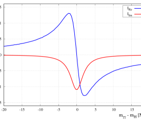
Figure 1: Real and imaginary parts of the signal-background interference terms, see text for details. This figure is just for illustration purposes. Our best prediction for these curves will be described in details in Sec. 4.

It is clear from these equations that the real part of the interference is an antisymmetric function of the diphoton invariant mass $m_{\gamma\gamma}^{2}$ around the Higgs resonance, and therefore does not contribute to the total cross-section. This is not the case for the imaginary part, which is instead symmetric around the resonance. This is illustrated in Fig. 1, where we plot $I_{\mathrm{Re}}$ and $I_{\mathrm{Im}}$ in the $gg$ channel up to NLO, to better visualise their independent effects.

Naively, one may think that the relative impact of the interference on the Higgs total cross section could be quite sizeable, since the signal is a two-loop process while the background starts at one loop. Because of this, one may expect a loop-enhancement factor of the interference with respect to the signal. However, a close inspection of Eq. (6) shows that the contribution to $I_{\mathrm{Im}}$ from the imaginary part of the background is strongly suppressed at leading order. This follows from the fact that the Higgs boson, being a scalar, only decays into a pair of photons with identical helicity. In turn, if the photons have equal helicities the imaginary part of the background at leading order vanishes, unless the process is mediated by a massive quark. In our calculation we keep full dependence on the bottom quark at leading order but, since its contribution is mass-suppressed, the net effect is small and can be safely neglected at higher orders. Starting from two loops, the relevant background helicity amplitudes develop an imaginary part. This leads to $I_{\mathrm{Im}}$ having a destructive impact of around $1$-$2\%$ Dixon:2003yb ; Campbell:2017rke . As far as the real part is concerned, there is no mass suppression at LO. Although such effect does not contribute to the total cross section, c.f. Eq. (6), it leads to a non-negligible shift of events around the diphoton invariant-mass peak, as it was first noted in Ref. Martin:2012xc .

Moreover, it was observed in Ref. Dixon:2013haa that the integrated interference $I$ has a different dependence on the Higgs boson production and decay couplings compared to the integrated signal. Specifically, if we schematically denote with $\lambda_{g}$ and $\lambda_{\gamma}$ the Higgs couplings to gluons and photons, we find that the signal is proportional to $\lambda_{g}^{2}\lambda_{\gamma}^{2}/\Gamma_{H}$, while the interference is only proportional to $\lambda_{g}\lambda_{\gamma}$. The main idea of Ref. Dixon:2013haa is to exploit this intertwined dependence on the Higgs boson couplings and its decay rate to extract information on $\Gamma_{H}$ and to look for possible deviations from its SM value. Current experimental measurements constrain the Higgs-diphoton rate to be the same of its SM prediction to within 10% ATLAS:2022qef ; ATLAS:2022fnp ; CMS:2022wpo . At this level of accuracy, one can neglect the small impact of the destructive interference $I_{\mathrm{Im}}$ on the cross section. One then schematically writes this experimental observation as

$$\frac{\lambda_{g}^{2}\lambda_{\gamma}^{2}}{\Gamma_{H}}\approx\displaystyle\frac{\lambda_{g,\rm SM}^{2}\lambda_{\gamma,\rm SM}^{2}}{\Gamma_{H,\rm SM}},$$ (7)

where $\lambda_{i}$, $\Gamma_{H}$ are the “true” Higgs-boson couplings and width and $\lambda_{i,\mathrm{SM}}$, $\Gamma_{H,\mathrm{SM}}$ are their respective SM predictions. Eq. (7) holds in particular under appropriate rescalings of $\lambda_{i,\mathrm{SM}}$ and $\Gamma_{H,\mathrm{SM}}$, e.g. $\lambda_{i}\to\kappa\lambda_{i,\mathrm{SM}}$ and $\Gamma_{H}\to\kappa^{4}\Gamma_{H,\mathrm{SM}}$, so it does not allow for a simultaneous direct extraction of couplings and width. However, if one supplements Eq. (7) with the observation that $I_{\mathrm{Re}}\propto\lambda_{g}\lambda_{\gamma}$, then one obtains

$$\frac{I_{\mathrm{Re}}}{I_{\mathrm{Re},\mathrm{SM}}}\propto\sqrt{\displaystyle\frac{\Gamma_{H}}{\Gamma_{H,\mathrm{SM}}}}.$$ (8)

Hence, a measurement of $I_{\mathrm{Re}}$ allows for an extraction of $\Gamma_{H}$, provided that the SM prediction $I_{\mathrm{Re},\mathrm{SM}}$ is under good theoretical control.

As mentioned before, the main effect of $I_{\mathrm{Re}}$ is to distort the Higgs invariant-mass distribution, effectively shifting the position of the peak. This translates into an apparent mass-shift with respect to the SM value Martin:2012xc . A measurement of such mass-shift can then be used to constrain $\Gamma_{H}$. In the next section, we review how one can extract the mass-shift from the knowledge of the Higgs invariant-mass distribution.

2.2 Extraction of the mass-shift

One first remark is that the Higgs resonance is extremely narrow, and therefore strongly smeared by the finite detector resolution. To properly take this into account, one should convolve theoretical prediction with a full detector simulation. However, such a study can only be carried out by experimental collaborations and it is outside the scope of this theoretical work. In this paper we estimate the mass-shift using two different, yet related, proxies for it that have been presented in the literature. Namely, we will consider the first moment of the diphoton invariant-mass distribution Martin:2012xc and a full gaussian fit to it Dixon:2013haa .

Before reviewing these techniques, we stress that they are inherently different, so one should not expect identical results for the mass shift. In other words, we can think of these procedures as a measurement of an observable that is strongly correlated, yet not identical, to the mass shift that experimentalists would measure. Nevertheless, we may imagine that they capture similar physics, and hence they should receive comparable radiative corrections. In Section 4, we will see that this is indeed the case. This gives us confidence that, even if our theoretical predictions for the absolute values of the mass shift are inherently limited by our experimental modeling, our results for the QCD $K$-factors are quite robust.

We now describe the two methods in some detail. In both cases, we simulate detector effects by smearing the diphoton invariant-mass distribution using a Gaussian function with $\sigma=1.7\leavevmode\nobreak\ \mathrm{GeV}$ ATLAS:2016kvj .

The first-moment method Martin:2012xc is based on the observation that, from the theoretical side, a very simple way to access the mass shift is to consider the first moment of the invariant-mass distribution, i.e.

$$\langle m_{\gamma\gamma}\rangle=\displaystyle\frac{1}{\sigma_{gg\to\gamma\gamma}}\int dm_{\gamma\gamma}m_{\gamma\gamma}\displaystyle\frac{d\sigma_{gg\to\gamma\gamma}}{dm_{\gamma\gamma}}$$ (9)

where $\sigma_{gg\to\gamma\gamma}$ is the fiducial cross-section. The mass shift is then defined as

$$\Delta m_{\gamma\gamma}=\langle m_{\gamma\gamma}\rangle_{\mathrm{sig+int}}-\langle m_{\gamma\gamma}\rangle_{\mathrm{sig}}.$$ (10)

The main advantage of this method is that it is theoretically very clean. Also, it is not very sensitive to overall normalisation issues, but rather focuses on the position of the peak. On the practical level however, it requires exquisite resolution on the invariant mass distribution which is very hard to achieve experimentally. It also strongly depends on the technical details of the theoretical analysis. For example, in Ref. Martin:2012xc the author found that the mass-shift strongly depends on the choice of the upper and lower integration boundaries in Eq. (9). Indeed, a change of $\mathcal{O}(1\,\mathrm{GeV})$ in such choice modifies the mass-shift estimate by almost $20\%$ at leading order.

A different proposal that addresses at least some of the shortcomings of the first-moment method is to simply perform a Gaussian fit of the diphoton invariant mass distribution Dixon:2013haa . One then extracts the mass shift by comparing predictions obtained with and without including interference effects. It was argued in Ref. Dixon:2013haa that this method is more resilient against specific details of analysis with respect to the first-moment one.

These two methods predict a mass-shift of $\mathcal{O}(100)\leavevmode\nobreak\ \mathrm{MeV}$ at LO. More precisely, the first-moment technique gives results in the interval $\Delta m_{\gamma\gamma}\in\{-250,-150\}\leavevmode\nobreak\ \mathrm{MeV}$ depending on the integration window in Eq. (9) Martin:2012xc . The likelihood fit of Ref. Dixon:2013haa instead predicts $\Delta m_{\gamma\gamma}=-120\leavevmode\nobreak\ \mathrm{MeV}$. As we have stressed before, these two methods measure correlated yet slightly different observables, so one should not expect identical results.

3 Higher-order QCD corrections

In this section, we present the technical details of our calculation. We start by discussing LO predictions for the interference. At order $\alpha_{s}^{2}$, we need to consider three different partonic channels, see Fig. 2 (top). We then write

$$\mathrm{LO}=\mathrm{LO(gg)}+\mathrm{LO(qg)}+\mathrm{LO(q\bar{q})}\,.$$ (11)

At this order, we compute the signal retaining the full top- and bottom- mass dependence. For the background, we neglect top-mediated contributions, since they are heavily suppressed. As we have explained in Section 2.1, the bottom-quark contributions are the only ones leading to a non-vanishing $I_{\mathrm{Im}}$ at this order. This effect is very small Campbell:2017rke , so we neglect it at higher orders. Because of this, when computing (N)NLO corrections we consider Higgs production in the heavy-top effective theory, described by the following Lagrangian

$$\mathcal{L}_{\mathrm{eff}}=-\frac{\lambda}{4}\,HG_{\mu\nu}^{a}G^{\mu\nu}_{a},$$ (12)

where $\lambda=-\alpha_{s}/(3\pi v)+\mathcal{O}(\alpha_{s}^{2})$ is the bare coupling and $v$ is the Higgs vacuum expectation value. At higher-orders, we still treat the Higgs decay to photons at LO, with exact mass dependence. Indeed, QCD radiative corrections are known to be small Djouadi:1990aj . For convenience, we report the relevant amplitude in A. As far as the background is concerned, we set the bottom mass to zero beyond LO.

It is well-known that the $gg$ channel is the dominant one for the signal process. For the interference, this statement is somehow weakened but still true. Indeed, the $qg$ channel (see Fig. 2) accounts for about 30% of the result deFlorian:2013psa . While it is easy with current technology to perform a full NLO analysis, in this paper we are mostly interested in the impact of NNLO corrections. We therefore focus our attention on the $gg$ channel only.

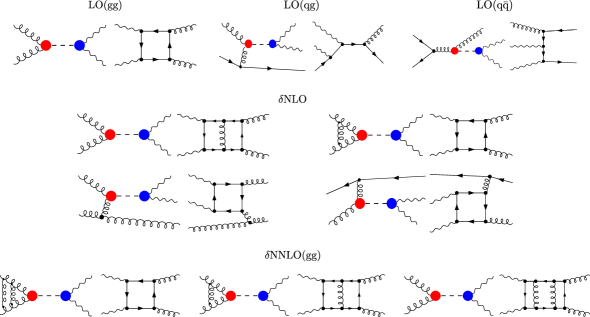
Figure 2: Representative diagrams contributing to the interference up to order $\alpha_{s}^{4}$. The red dot denotes the effective vertex described through the Lagrangian in Eq. (12), while the blue dot denotes the Higgs decay via heavy quark loops and W boson, described in Eq. (24).

Strictly speaking, if we include only gluon-induced processes, NLO corrections are given by only the first three out of the four $\delta\mathrm{NLO}$ diagrams of Fig. 2. Of course, this would imply that one should evolve parton distribution functions (PDFs) in the same approximation. However, one can also retain formally subleading effects. In particular, the quark-induced contribution in the third row of Fig. 2 is linked to the $gg$ channel through PDF evolution. One may then expect that its inclusion in the DGLAP evolution of the PDFs would alleviate the factorisation-scale dependence of the result. Therefore, following Ref. Dixon:2013haa , in our analysis we use standard parton distributions and include the last diagram in the third row of Figure. 2. In what follows, we call ‘$\delta$NLO’ the contribution coming from the second and third rows of that figure. We stress that this is not the full NLO correction to the interference. It may also be instructive to consider only gluon-induced diagrams at this order. Indeed, comparing this against our default setup may give us a handle on the large-gluon approximation. In what follows, we define corrections computed using only the first three diagrams of the block of diagrams ($\delta$NLO) in Fig. 2 as ‘$\delta$NLO(gg)’. Correspondingly we call the the full NLO result

$$\mathrm{NLO}=\mathrm{LO}+\delta\mathrm{NLO},\leavevmode\nobreak\ \leavevmode\nobreak\ \mathrm{NLO}(gg)=\mathrm{LO}+\delta\mathrm{NLO}(gg),$$ (13)

with $\mathrm{LO}$ defined in Eq. (11).

We now move to NNLO corrections. As we have said, at this order we work in the soft-virtual approximation. This is justified by the fact that, at least at lower orders, interference effects are stronger in the region where the diphoton transverse momentum is small Martin:2013ula ; Dixon:2013haa . The soft-virtual approximation and various refinements of it have been extensively adopted for Higgs predictions Catani:2001ic ; Moch:2005ky ; Ball:2013bra ; deFlorian:2014vta ; Anastasiou:2014vaa . The main advantage of working in this limit is that the only process-dependent part is encoded in purely virtual contributions, see e.g. Ref. deFlorian:2012za for an explicit derivation.

Here we only sketch the structure of the soft-virtual approximation, and refer the reader to Ref. deFlorian:2012za for more details. We write the fully-differential hadronic cross section for diphoton production in the $gg$ channel as

$$d\sigma(\tau,y,\{\theta_{i}\})=\int d\xi_{1}d\xi_{2}dzf_{g}(\xi_{1},\mu_{F})f_{g}(\xi_{2},\mu_{F})$$

$$\times\,\delta(\tau-\xi_{1}\xi_{2}z)d\hat{\sigma}\left(z,\hat{y},\{\hat{\theta}_{i}\},\alpha_{s},\displaystyle\frac{Q^{2}}{\mu_{R}^{2}},\displaystyle\frac{Q^{2}}{\mu_{F}^{2}}\right).$$ (14)

In this equation, $\tau=Q^{2}/s_{\rm had}$ with $Q$ being the invariant mass of the diphoton system and $s_{\rm had}$ the square of the collider energy, $y$ is the rapidity of the diphoton system in the laboratory frame and $\theta_{i}$ are a set of variable that fully describe the diphoton system (e.g. scattering angles). Variables with hats represent the corresponding partonic quantities. Eq. (14) is fully differential in the kinematics of the diphoton system, but retain no information on extra QCD radiation. We note that the partonic variables $\{\hat{\theta}_{i}\}$ depend on their hadronic counterparts $\{\theta_{i}\}$ and also on $z,\xi_{1},\xi_{2}$. Finally, $\alpha_{s}=\alpha_{s}(\mu_{R})$ is the renormalised QCD coupling constant evaluated at scale $\mu_{R}$.

Major simplifications occur in the soft $z\to 1$ limit. First, in this case the rapidity dependence of Eq. (14) is entirely fixed by the inclusive cross section, up to power corrections Bolzoni:2006ky ; Becher:2007ty ; Bonvini:2010tp . The partonic cross section in Eq. (14) simplifies to

$$d\hat{\sigma}\left(z,\hat{y},\{\hat{\theta}_{i}\},\alpha_{s},\displaystyle\frac{Q^{2}}{\mu_{R}^{2}},\displaystyle\frac{Q^{2}}{\mu_{F}^{2}}\right)\approx$$

$$d\hat{\sigma}_{\rm Born}(\{\hat{\theta}_{i}\},\alpha_{s})\,z\,G\left(z,\alpha_{s},\displaystyle\frac{Q^{2}}{\mu_{R}^{2}},\displaystyle\frac{Q^{2}}{\mu_{F}^{2}}\right),$$ (15)

where we neglected power corrections in $(1-z)$. In Eq. (15), $d\sigma_{\rm Born}(\{\hat{\theta}_{i}\},\alpha_{s})\delta(1-z)$ is the Born cross section and $G$ is the inclusive coefficient function in the soft limit, normalised such that $G=\delta(1-z)+\mathcal{O}(\alpha_{s})$. In the soft limit, the diphoton kinematics is identical to the LO one, except that the partonic center-of-mass energy is rescaled by $z$. Such a rescaling factor can be absorbed by boosting an individual leg, i.e. by using the partonic momenta $\xi_{1,\rm Born}\to z\,\xi_{1,\rm Born},\xi_{2,\rm Born}\to\xi_{2,\rm Born}$ (and vice versa). Alternatively, one can boost both legs at the same time, i.e. $\xi_{i,\rm Born}\to\sqrt{z}\,\xi_{i,\rm Born}$, $i=1,2$. In the soft-limit, the two are formally equivalent and, in principle, one can consider both and treat their difference as an uncertainty. In practice, we expect this difference to be small Bonvini:2013jha , so for simplicity we always boost only one leg in this work.

If we write the perturbative expansion of the coefficient function as

$$G\left(z,\alpha_{s}\right)=\delta(1-z)+\sum_{n=1}^{\infty}\left(\displaystyle\frac{\alpha_{s}}{2\pi}\right)^{n}G^{\left(n\right)}(z),$$ (16)

then in the soft-virtual approximation the individual coefficients $G^{(n)}$ have the form

$$G^{(n)}\left(z,\displaystyle\frac{Q^{2}}{\mu_{R}^{2}},\displaystyle\frac{Q^{2}}{\mu_{F}^{2}}\right)=c_{0}\delta(1-z)+\sum_{k=1}^{2n-1}c_{k}\mathcal{D}_{k}(z),$$ (17)

where $c_{k}=c_{k}(Q^{2}/\mu_{R}^{2},Q^{2}/\mu_{F}^{2})$ and $\mathcal{D}_{k}$ are the standard plus distributions

$$\mathcal{D}_{k}(z)=\left[\frac{\ln^{k}(1-z)}{1-z}\right]_{+}.$$ (18)

We present explicit formulas for the NLO and NNLO coefficients, retaining full scale dependence, in B. The coefficients $c_{k}$ in Eq. (17) in principle depend on the process under consideration. However, it turns out that the only process dependence arises from finite remainders of purely virtual contributions and it is therefore encoded in the coefficient $c_{0}$. As a consequence, the coefficients of the plus distributions are completely process-independent.

For the analysis in the next section, we also require the signal process at NNLO accuracy. In principle, computing this exactly does not pose significant challenges. Nevertheless, we expect the exact result to be very well described by a (refined) version of the soft-virtual approximation Catani:2001ic ; Moch:2005ky ; Ball:2013bra ; deFlorian:2014vta . While the pure soft-virtual prediction provides a good approximation to the interference, this is not the case for the signal. We therefore employ a modified soft-virtual approximation to describe the latter. Specifically, we follow the approach of Ref. Ball:2013bra which is known to reproduce the exact NNLO prediction to within few-percent accuracy. In practice, this amounts to modifying the plus distributions in Eqs. (B,B) according to Ball:2013bra

$$\mathcal{D}_{i}(z)\to\mathcal{D}_{i}(z)+(2-3z+2z^{2})\frac{\ln^{i}\frac{1-z}{\sqrt{z}}}{1-z}-\frac{\ln^{i}(1-z)}{1-z}.$$ (19)

This modification captures soft emission at next-to-leading power, as well as part of the hard collinear emission. Such an approximation was already used for estimating signal-background interference effects for the $gg\to VV$ process Bonvini:2013jha . In our case, we have specifically checked that for on-shell Higgs, within the fiducial volume used in our analysis, the soft-virtual approximation improved according to Eq. (19) agrees with the exact NNLO result to within few percent. This is good enough for the kind of accuracy targeted in our analysis. In the following section, we will refer to this improved soft-virtual approximation as “$\mathrm{NNLOsv\textquotesingle}$”. The reason why we do not adopt such an improved approximation for the background is because it is currently unknown how to properly capture next-to-leading power soft term in this case. Indeed, a simple modification of emission off external legs works for the Higgs point-like interaction, but not for the background amplitude. Fortunately, the interference seems to be dominated by low-$p_{T}$ physics so the lack of such an improved approximation is less problematic than for the signal.

We conclude this section by listing the various ingredients of our calculation. The LO amplitudes, including the quark-mass effects, are well known, see e.g. Ellis:1996mzs and references therein. At NLO, we took the one-loop amplitudes for the background from Refs. Bargiela:2021wuy ; Campbell:2016yrh ; Bern:2002jx ; Agarwal:2021vdh , borrowing most of them from MCFM Campbell:1999ah ; Boughezal:2016wmq ; Campbell:2019dru . We note that the two-loop amplitude for $gg\to\gamma\gamma$ was first computed in Ref. Bern:2001df . NLO predictions were computed using FKS subtraction Frixione:1995ms . Finally, the three-loop $gg\to\gamma\gamma$ amplitude relevant for NNLO corrections was taken from Ref. Bargiela:2021wuy . All the tree- and one-loop results for the interference were cross-checked against a dedicated version of OpenLoops2 Buccioni:2019sur ; Cascioli:2011va .

4 Results

In this section, we discuss our main findings. We start by specifying the setup we are using.

We employ the so-called $G_{\mu}$ input scheme for the electroweak parameters and we use

$$G_{F}=1.16639\cdot 10^{-5}\leavevmode\nobreak\ \mathrm{GeV}^{-2}\,,$$

$$m_{W}=80.398\leavevmode\nobreak\ \mathrm{GeV},\quad m_{Z}=91.1876\leavevmode\nobreak\ \mathrm{GeV}$$

that give the electroweak coupling constant $\alpha=1/132.338$. We set the Higgs mass to $m_{H}=125\leavevmode\nobreak\ \mathrm{GeV}$. Finally, we use $m_{t}=173.2\leavevmode\nobreak\ \mathrm{GeV}$ and $m_{b}=4.18\leavevmode\nobreak\ \mathrm{GeV}$ for the top and bottom mass, respectively. We use the NNPDF31_nnlo_as_0118 NNPDF:2017mvq parton distribution functions as distributed through the LHAPDF library Buckley:2014ana and we use Hoppet Salam:2008qg for various PDFs manipulations. The value of the strong coupling costant is extracted from the PDF set, with $\alpha_{s}(m_{Z})=0.118$. For the QCD factorisation and renormalisation scales, we choose the common value $\mu_{F}=\mu_{R}=m_{\gamma\gamma}/2$, where $m_{\gamma\gamma}$ is the invariant mass of the diphoton system. All of the results presented in this section have been derived for the $13.6\leavevmode\nobreak\ \mathrm{TeV}$ LHC, i.e. proton-proton collisions. We define the fiducial region by imposing the following set of cuts on the final-state photons

$$p_{T,\gamma}>20\,\mathrm{GeV},\quad\quad\sqrt{p_{T,\gamma_{1}}p_{T,\gamma_{2}}}>35\,\,\mathrm{GeV},$$

$$\qquad|y_{\gamma}|<2.5,\quad\quad\Delta R_{\gamma_{1}\gamma_{2}}>0.4,\;$$ (20)

which are designed to reduce sensitivity on infrared physics Salam:2021tbm . The cuts in Eq. (4) are different from the ones used in Refs. Dixon:2013haa ; deFlorian:2013psa . Because of this, it is not immediate to compare our results with the ones presented there. Nevertheless, we have validated our LO and NLO calculations against Refs. Dixon:2013haa ; deFlorian:2013psa . In particular, we have reproduced the results for the mass shift shown in Refs. Dixon:2013haa ; deFlorian:2013psa . We have also used MCFM Campbell:1999ah ; Boughezal:2016wmq ; Campbell:2019dru , together with in-house codes, to validate the signal and the reliability of the $\mathrm{NNLOsv\textquotesingle}$ approximation.

We start the discussion of our results by assessing the validity of the soft-virtual approximation for the interference at NLO. We do this by first comparing the exact prediction including only the $gg$ initiated process, which we dub $\mathrm{NLO}(\mathrm{gg})$, to the corresponding soft-virtual approximation, $\mathrm{NLOsv}(\mathrm{gg})$.

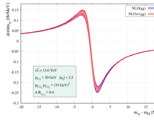
Figure 3: Left pane: comparison of the exact NLO calculation and the soft-virtual approximation in the $gg$ channel. Right pane: complete NLO prediction, inclusive of all channels, compared to the corresponding soft-virtual approximation

This comparison is shown in the left pane of Fig. 3. Second, we compare the complete NLO calculation, i.e. including the $qg$ and $\bar{q}g$ initiated channels  to the NLO soft-virtual approximation ($\mathrm{NLOsv}$), which retains all LO contributions, but includes NLO corrections in the soft-virtual approximation for the $gg$ channel only. This comparison is presented in the right pane of Fig. 3. The red and blue bands shown in both figures represent the envelope from a simultaneous rescaling of $\mu_{F,R}$ by a factor of two up and down with respect to the central value. We note that our result suggests that the uncertainty due to scale variations does not provide a reliable estimate of the actual error of the NLO prediction. In the left pane of Fig. 3 one can see that the soft-virtual approximation does a remarkably good job in describing the dominant $gg$ contribution. The shape of the interference is very well captured and the scale-variation bands almost perfectly match throughout the relevant interval of invariant mass. In the right side of Fig. 3 we notice a slight degrading of the approximation, mostly for what concerns the scale variation bands. This is because the soft-virtual approximation does not capture the full scale-compensation between different channels that happens at NLO. However, the shape, which is the relevant factor for the extraction of the mass-shift, is still described at a satisfactory degree.

This comparison gives us some confidence that the soft-virtual approximation can adequately describe higher-order QCD corrections to the signal-background interference. Furthermore, we note that the mass-shift extracted at NLO in the soft-virtual approximation differs from the exact value by $5\%$, whilst the genuine NLO correction is of $\mathcal{O}(30/40\%)$ and the theory uncertainty is $\mathcal{O}(10\%)$. The ability of the soft-virtual approximation in reproducing the interference effects can be better understood by keeping in mind that the predominant contributions come from the low $p_{T,\gamma\gamma}$ regions, as we already mentioned in Sec. 1. We point out that the fiducial setup adopted in Eq. (4), in particular with the choice of product cuts, plays a relevant role in the reliability of the soft-virtual approximation. We have indeed explicitly checked that imposing asymmetric cuts on the final-state photons, as it is routinely done in Higgs analysis, breaks the quality of the approximation.

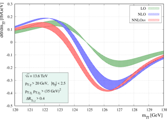
Figure 4: Signal-background interference contribution to the diphoton invariant mass distribution after Gaussian smearing. Bands represent the envelope given by the scale variation.

As already discussed in Sec. 2.2, in order to get a more realistic picture of the interference effect at the detector level, we convolute the invariant mass distribution with a Gaussian function with a standard deviation of $\sigma=1.7\leavevmode\nobreak\ \mathrm{GeV}$ Martin:2012xc ; ATLAS:2016kvj

The invariant mass distribution arising from signal-background interference after the smearing is shown in Fig. 4. The LO features the well known antisymmetric behaviour around the peak coming from the real part of the interference, whereas the NLO curve is shifted to the left and to the bottom, due to the impact of the imaginary part. In the same figure, we can appreciate for the first time the effect of the NNLO QCD corrections. The curve is further shifted down, thus depleting even more the number of events around the Higgs peak and softening the impact on the mass-shift.

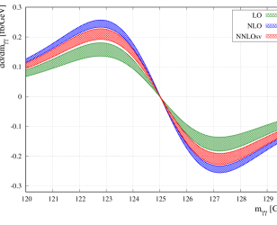
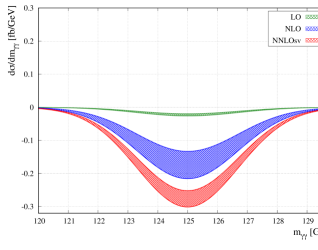
Figure 5: Real part (left pane) and imaginary part (right pane) of the interference at LO, NLO and NNLOsv after Gaussian smearing.

Moreover, from Fig. 4 one can see that the theory uncertainty, which arises almost completely from renormalisation scale variations, gets generally reduced at NNLO, except in the region where the NLO band shrinks to zero. This behaviour can be understood keeping in mind that the interference is the sum of the real and imaginary parts which have different shapes, as discussed in Sec. 2.1. As shown in Fig. 5, scale-variation bands are separately well behaved for the real and imaginary parts, but on the left hand side of the Higgs boson peak a cancellation occurs, whereas on the right the two effects sum up (both negative in sign).

Before moving to our results for the mass shift, we briefly discuss the impact of the imaginary part of the interference to the total cross section in our fiducial region. As we have explained in Sec. 2.1, at LO this interference is very small because it only comes from contributions mediated by virtual bottom quarks, either in the signal or in the background. These are either mass (background) or Yukawa (signal) suppressed. The smallness of the LO imaginary part is indeed seen in Fig. 5. In our setup, we find

$$\sigma_{S}^{\mathrm{LO}}=24.21^{+15\%}_{-14\%}\leavevmode\nobreak\ \mathrm{fb},\leavevmode\nobreak\ \leavevmode\nobreak\ \leavevmode\nobreak\ \leavevmode\nobreak\ \leavevmode\nobreak\ \leavevmode\nobreak\ \sigma_{I}^{\mathrm{LO}}=-0.11^{+20\%}_{-17\%}\leavevmode\nobreak\ \mathrm{fb}.$$ (21)

Here and in the following the quoted uncertainties are obtained by coherently varying the renormalisation and factorisation scales by a factor of two around the central value $\mu=m_{\gamma\gamma}/2$. At LO, we find that more than 80% of the destructive interference quoted above comes from the imaginary part of the signal interfering with the real part of the background. This gives us confidence that neglecting mass effects in the background prediction does not significantly impact our result. Furthermore, as far as the signal goes, we note that the bulk (about 95%) of the imaginary part is generated by bottom-mass effects in the production amplitude. This is easy to understand just by looking at the relative importance of the top, bottom and $W$ contributions to the production and decay amplitudes.

At higher orders however, a larger interference is generated by the imaginary part of the background, which no longer requires the presence of bottom quarks (see the discussion in Sec. 3). Because of this, beyond LO we only compute radiative corrections in the infinite-top approximation and drop any mass dependence in the background amplitudes. At NLO, we obtain

$$\sigma_{S}^{\mathrm{NLO}}=58.12^{+20\%}_{-14\%}\leavevmode\nobreak\ \mathrm{fb},\leavevmode\nobreak\ \leavevmode\nobreak\ \leavevmode\nobreak\ \leavevmode\nobreak\ \leavevmode\nobreak\ \leavevmode\nobreak\ \sigma_{I}^{\mathrm{NLO}}=-0.72^{+27\%}_{-21\%}\leavevmode\nobreak\ \mathrm{fb}.$$ (22)

These results are consistent with the analysis in Ref. Campbell:2017rke . Our best prediction beyond NLO is obtained within the soft-virtual approximation described in Sec. 3. We find

$$\sigma^{\mathrm{NNLOsv}^{\prime}}_{S}=72.21^{+8\%}_{-8\%}\;\mathrm{fb},\leavevmode\nobreak\ \leavevmode\nobreak\ \leavevmode\nobreak\ \leavevmode\nobreak\ \sigma^{\mathrm{NNLOsv}}_{I}=-1.21^{+7\%}_{-10\%}\;\mathrm{fb},$$ (23)

hence the destructive interference reduces the total rate by $1.7\%$. Given the theoretical LHCHiggsCrossSectionWorkingGroup:2016ypw (see also Refs. Giulia ; Robert ) and experimental ATLAS:2022fnp ; CMS:2022wpo uncertainty on the Higgs total cross section, this effect is actually not negligible and it can be used to further constrain the Higgs width Campbell:2017rke . We do not pursue this line of investigation here, but we estimate that, with current uncertainties, one could already constrain the Higgs width to about 20-30 times the Standard Model.

$\Delta m_{\gamma\gamma}\left[\text{MeV}\right]$	7 TeV	8 TeV	13.6 TeV
$\mathrm{LO}$	$-77.2_{-1.0\%}^{+0.8\%}$	$-79.5_{-0.8\%}^{+0.6\%}$	$-83.1^{+0\%}_{-0.3\%}$
$\mathrm{NLO}$	$-56.2_{-15\%}^{+13\%}$	$-56.8_{-14\%}^{+13\%}$	$-55.2_{-12\%}^{+12\%}$
$\mathrm{NNLOsv}$	$-46.3_{-17\%}^{+15\%}$	$-47.0_{-16\%}^{+14\%}$	$-46.0_{-12\%}^{+11\%}$
$\mathrm{NNLOsv\textquotesingle}$	$-39.5_{-24\%}^{+20\%}$	$-39.7_{-22\%}^{+19\%}$	$-39.4_{-17\%}^{+16\%}$

Table 1: Mass-shift at different proton-proton collider energies with Gaussian fit method.

$\Delta m_{\gamma\gamma}\left[\text{MeV}\right]$	7 TeV	8 TeV	13.6 TeV
$\mathrm{LO}$	$-113.4_{-1.0\%}^{+0.8\%}$	$-116.7_{-0.8\%}^{+0.6\%}$	$-122.1_{-0.3\%}^{+0.1\%}$
$\mathrm{NLO}$	$-82.6_{-15\%}^{+13\%}$	$-82.8_{-14\%}^{+12\%}$	$-81.2_{-12\%}^{+12\%}$
$\mathrm{NNLOsv}$	$-68.1_{-17\%}^{+15\%}$	$-68.4_{-15\%}^{+13\%}$	$-67.7_{-12\%}^{+11\%}$
$\mathrm{NNLOsv\textquotesingle}$	$-58.1_{-23\%}^{+20\%}$	$-59.2_{-21\%}^{+18\%}$	$-58.0_{-17\%}^{+16\%}$

Table 2: Mass-shift at different proton-proton collider energies with first moment method.

We can finally present the main result of our study, i.e. the prediction for the mass-shift at NNLO. As discussed in Sec. 2.1, we adopt two different methods to estimate the mass-shift induced by the interference term. In Table 2 we show the results obtained by performing a chi-squared fit of the smeared signal-plus-interference distribution with a Gaussian function of standard deviation $\sigma=1.7\,\mathrm{GeV}$. The mass-shift is obtained as the difference between the obtained mean value and the input Higgs boson mass $m_{H}=125\leavevmode\nobreak\ \mathrm{GeV}$. In Table 2 instead we present results derived by computing the first moment of the signal-plus-interference distribution after smearing. In both tables we show predictions for different collider energies, but in the same fiducial region specified in Eq. (4). As mentioned earlier, the denoted ranges represent the theoretical uncertainty related to a change of the central scale $\mu=m_{\gamma\gamma}/2$ by a factor of two and a half. The entry $\mathrm{NNLOsv}$ indicates the result obtained by considering both signal and interference terms in the soft-virtual approximation. The $\mathrm{NNLOsv\textquotesingle}$ entry instead, refers to the “improved” soft-virtual approximation discussed at the end of Sec. 3. Specifically, in this case we still use the $\mathrm{NNLOsv}$ approximation for the interference, but compute the signal in the $\mathrm{NNLOsv\textquotesingle}$ framework. As we explained in Sec. 3, we expect this setup to be the most realiable one. Still, we find it useful to present numbers in both frameworks as a conservative way of estimating the uncerainties related to these approximations. In this respect, we note that the results obtained in the $\mathrm{NNLOsv}$ and $\mathrm{NNLOsv\textquotesingle}$ approximations are compatible within their uncertainties.

We immediately notice that in both extraction methods, the estimated mass-shift is rather insensitive to the collider energy.

$\Delta m_{\gamma\gamma}\left[\text{MeV}\right]$	First moment	Gaussian Fit
$K_{\mathrm{NLO}}$	0.665	0.664
$K_{\mathrm{NNLOsv}}$	0.554	0.554
$K_{\mathrm{NNLOsv\textquotesingle}}$	0.475	0.474

Table 3: Comparison of $K$-factors, measured w.r.t. the LO value, for the mass-shift at $\sqrt{s}=13.6\leavevmode\nobreak\ \mathrm{TeV}$ calculated via a gaussian fit method and via a first-moment method.

Although a Gaussian fitting procedure and the evaluation of the first moment return different values for the mass-shift, smaller for the former and larger for the latter, we notice that the $K$-factors relative to the corresponding LO prediction are almost identical. We stress that this is a welcome feature since our analysis does not include reliable detector simulation. The results in Table 3 show that radiative corrections seem rather insensitive to the precise definition of the observable used to extract the mass shift.

We also observe how the mass-shift gets systematically reduced in absolute value when including higher-order corrections. This is mainly because the $K$-factor for the signal turns out to be larger than the one for the interference, thus leading to a reduction of the mass-shift. This trend, already observed at NLO Dixon:2013haa , seems to persist at NNLO (at least in the $\mathrm{NNLOsv}$ approximation).

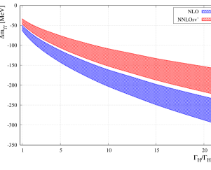
Figure 6: Mass-shift as a function of the Higgs boson width

Finally, we study how the bounds on $\Gamma_{H}$ are affected by higher-order QCD corrections, following the discussion at the end of Sec. 2.1. The results at NLO and $\mathrm{NNLOsv\textquotesingle}$ (i.e. our best prediction) are shown in Fig. 6. Our NLO curve is compatible with the one obtained in Dixon:2013haa . We note that the two curves do not overlap. This is a direct consequence of the analogous feature for the interference shown in Fig. 4. As explained in the comment of that figure, this is at least partially due to competing effects coming from real and imaginary part of the interference, see Fig. 5. Furthermore, similar to the Higgs-signal case, the interference receives rather large corrections as well. Finally, we note that the NNLO soft-virtual curve lies above the NLO one, thus loosening potential bounds on $\Gamma_{H}$. For instance, if at the LHC the error on the mass-shift reaches roughly $150\leavevmode\nobreak\ \mathrm{MeV}$, one could exclude values of $\Gamma_{H}$ larger than 10–20 times the SM prediction. This has to be compared with the corresponding bound at NLO of $\Gamma_{H}<(6\text{--}9)\Gamma_{H,\mathrm{SM}}$.

5 Conclusions

We presented a calculation of the NNLO soft-virtual corrections to signal-background interference for gluon-fusion Higgs production in the diphoton channel at the LHC. More specifically, we focused on the shift in the diphoton invariant mass distribution which arises from the inclusion of the interference between the Higgs-mediated process and its continuum background, as first observed in Ref. Martin:2012xc . Such a study was only known up to NLO QCD so far Dixon:2013haa , due to unavailability of the relevant background amplitudes.

Recent developments in multi-loop scattering amplitudes techniques enabled the computation of such amplitudes Bargiela:2021wuy ; Agarwal:2021vdh ; Badger:2021imn . We were therefore able to extend this study one order higher in perturbation theory. We employed the soft-virtual approximation, motivated by previous studies which showed how the contribution to the mass-shift is enhanced in the low $p_{T,\gamma\gamma}$ region, and therefore dominated by virtual corrections and soft emissions. We have validated this approximation at NLO and shown that indeed it seems to capture the bulk of the corrections, to within few percent. We stress that this statement holds in our fiducial volume, which is designed to avoid spurious sensitivity to infrared physics Salam:2021tbm . Using more standard asymmetric cuts at fixed order, instead, would lead to a deterioration of the quality of the soft-virtual approximation.

We calculated the mass-shift by means of two different methods and found that, despite the absolute value being dependent on the observable chosen for its extraction, the $K$-factors for the NNLO soft-virtual corrections are very similar in both cases. Specifically, we found that the mass-shift further decreases at NNLO soft-virtual, confirming the trend already observed at NLO QCD. Within our approximation, we find that NNLO corrections are large, and amount to a decrease of almost 30% on top of the NLO prediction. Furthermore, these corrections are not captured by the standard scale variation band of the NLO prediction.

We used our results to obtain an updated prediction for the bounds that can be put on $\Gamma_{H}$ as a result of the mass-shift determination. We observed that the decrease in the mass-shift prediction results in a loosening of such bounds. If we estimate the experimental error on the mass shift to drop to $\mathcal{O}(150\leavevmode\nobreak\ \mathrm{MeV})$, we find that the Higgs boson width can be constrained to $\Gamma_{H}\lesssim(10-20)\Gamma_{H,SM}$. Interestingly, we find that the imaginary part of the interference instead grows with the perturbative order. Hence, it leads to a shift of the total cross section that could be used to extract information on the Higgs total width as well Campbell:2017rke . Although a detailed extraction based on this is beyond the scope of this paper, we estimate that with the current experimantal and theoretical uncertainties one could bound the Higgs width to within 20-30 times its Standard Model value.

There are several avenues for improving our predictions. First, one could perform an exact NNLO study. As we already mentioned, the main complication of such a calculation is a purely technical one, namely the numerical control of two-loop 5-point amplitudes (as well as 6-point one-loop ones) near singular contributions. Although we believe that our calculation captures the bulk of NNLO corrections, such an exact result would allow for a better modeling of the $p_{T}$-dependence of the interference, which would provide useful information for an actual extraction of the mass-shift. Indeed, the $p_{T}$ dependence of the result can be used to define signal and control regions to extract the mass shift within the diphoton channel alone thus minimising systematic uncertainties.

From a theoretical point of view, perhaps an even more interesting line of investigation would be to understand how to improve the soft-virtual approximation for the background amplitude. This would require improving our understanding of next-to-leading power soft corrections to cope with the case at hand. We leave these avenues for future work.

Appendix A Details on the signal amplitude

In this appendix we provide some details regarding our treatment of the Higgs signal amplitudes. For the decay component of the amplitude, we retain full dependence on the heavy quark masses at LO and neglect higher order radiative corrections. More specifically, we consider both quark and W-boson loops contributions,

$$\mathcal{A}_{H\gamma\gamma}=$$ (24)

$$-\displaystyle\frac{\alpha_{em}}{4\pi v}m_{\gamma\gamma}^{2}\Big{[}I_{W}\left(\displaystyle\frac{m_{W}^{2}}{m_{\gamma\gamma}^{2}}\right)+\sum_{q=b,t}N_{c}Q_{q}^{2}I_{q}\left(\displaystyle\frac{m_{q}^{2}}{m_{\gamma\gamma}^{2}}\right)\Big{]}$$

where $N_{c}$ is the number of colors in the fundamental representation of SU(3), $Q_{q}^{2}$ is the quark electric charge in units of the proton charge and

$$I_{W}(x) =-2[6x+1+6x(2x-1)F(x)]$$

$$I_{q}(x) =4x[2+(4x-1)F(x)]$$

$$F(x) =\theta(1-4x)\displaystyle\frac{1}{2}\Big{[}\log\left(\displaystyle\frac{1+\sqrt{1-4x}}{1-\sqrt{1-4x}}\right)-i\pi\Big{]}^{2}$$

$$-\theta(4x-1)2\left(\sin^{-1}\left(\displaystyle\frac{1}{2\sqrt{x}}\right)\right)^{2}\,.$$ (25)

As mentioned in Sec. 3, Higgs production is treated exactly at LO while the heavy-top effective field theory is employed at higher orders. In the case of exact top and bottom mass dependence, the expression for the production amplitude is

$$\mathcal{A}_{ggH}=-\displaystyle\frac{\alpha_{s}}{4\pi v}\frac{m_{\gamma\gamma}^{2}}{2}\,\sum_{q=b,t}Q_{q}^{2}I_{q}\left(\displaystyle\frac{m_{q}^{2}}{m_{\gamma\gamma}^{2}}\right)\,.$$ (26)

In the heavy-top effective theory, the Higgs production amplitude is described by the Lagrangian in Eq. (12). The effective coupling $\lambda$ reads

$$\lambda=-\displaystyle\frac{\alpha_{s}}{3\pi v}C(\alpha_{s})Z_{\lambda}(\alpha_{s})\,,$$ (27)

with $Z_{\lambda}(\alpha_{s})$ and $C(\alpha_{s})$ in the $\overline{\mathrm{MS}}$ scheme given by

$$Z_{\lambda}(\alpha_{s}) =1-\displaystyle\frac{\beta_{0}}{\epsilon}\left(\displaystyle\frac{\alpha_{s}(\mu)}{2\pi}\right)+\Big{[}\displaystyle\frac{\beta_{0}^{2}}{\epsilon^{2}}-\displaystyle\frac{\beta_{1}}{\epsilon}\Big{]}\left(\displaystyle\frac{\alpha_{s}(\mu)}{2\pi}\right)^{2}$$

$$+\mathcal{O}(\alpha_{s}^{3}),$$ (28)

$$C(\alpha_{s}) =1+\Big{[}\displaystyle\frac{5}{2}C_{A}-\displaystyle\frac{3}{2}C_{F}\Big{]}\left(\displaystyle\frac{\alpha_{s}(\mu)}{2\pi}\right)+\Big{[}\displaystyle\frac{1063}{144}C_{A}^{2}$$

$$-\displaystyle\frac{25}{3}C_{A}C_{F}+\displaystyle\frac{27}{8}C_{F}^{2}-\displaystyle\frac{47}{72}C_{A}n_{f}-\displaystyle\frac{5}{8}C_{F}n_{f}$$

$$-\displaystyle\frac{5}{48}C_{A}-\displaystyle\frac{C_{F}}{6}+\log\displaystyle\frac{\mu^{2}}{m_{t}^{2}}\Big{(}\displaystyle\frac{7}{4}C_{A}^{2}-\displaystyle\frac{11}{4}C_{A}C_{F}$$

$$+C_{F}n_{f}\Big{)}\Big{]}\left(\displaystyle\frac{\alpha_{s}(\mu)}{2\pi}\right)^{2}+\mathcal{O}(\alpha_{s}^{3}),$$ (29)

see e.g. Ref. Grigo:2014jma . In the equation above we use

$$\beta_{0}=\displaystyle\frac{11}{6}C_{A}-\displaystyle\frac{2}{3}n_{f}T_{R}$$

$$\beta_{1}=\displaystyle\frac{17}{6}C_{A}^{2}-\displaystyle\frac{5}{3}C_{A}T_{R}n_{f}-C_{F}T_{R}n_{f}$$ (30)

and $\alpha_{s}(\mu)$ is the renormalized coupling. The 1-loop and 2-loop gluon form factors which are relevant for the calculation of NLO and NNLO corrections to the signal amplitude have been taken from Ref. Gehrmann:2005pd .

Appendix B Soft-virtual cross-section at NLO and NNLO

In Section 3 we saw that the soft-virtual approximation consists in retaining only soft and virtual contributions to the cross-section and neglect hard and collinear contributions. In this appendix, we will define the various virtual contributions and present formulas for the soft-virtual cross-section for color singlet production at NLO and NNLO. As mentioned in Section 3, the soft-virtual cross-section is completely universal for a given partonic channel. We will present results for the $gg$-channel, since it is the one of interest for this work. The only process-dependent component is encoded in the virtual contributions. The NLO virtual contribution to the cross-section can be written as

$$\hat{\sigma}^{\mathrm{1-loop}}=\displaystyle\frac{\alpha_{s}(\mu)}{2\pi}I_{12}(\epsilon)\hat{\sigma}_{\mathrm{Born}}+\hat{\sigma}^{\mathrm{1-loop}}_{\mathrm{fin}}$$ (31)

where $\hat{\sigma}^{\mathrm{1-loop}}_{\mathrm{fin}}$ is the contribution to the cross section due to the interference of the finite remainder of the one-loop amplitude with the Born amplitude, and $I_{12}(\epsilon)$ is the Catani operator

$$I_{12}(\epsilon)=-2\cos(\pi\epsilon)\displaystyle\frac{e^{\epsilon\gamma_{E}}}{\Gamma(1-\epsilon)}\left(\displaystyle\frac{\mu^{2}}{s_{12}}\right)^{\epsilon}\left[\displaystyle\frac{C_{g}}{\epsilon^{2}}+\displaystyle\frac{\gamma_{g}}{\epsilon}\right]$$ (32)

with $C_{g}=C_{A}$ and $\gamma_{g}=\beta_{0}$. The NLO soft-virtual cross section then reads

$$G^{(1)}(z)=\delta(1-z)\left(\displaystyle\frac{2}{3}\pi^{2}+\displaystyle\frac{\hat{\sigma}^{\mathrm{1-loop}}_{\mathrm{fin}}}{\hat{\sigma}_{\mathrm{Born}}}-2\beta_{0}\log\displaystyle\frac{{\mu^{2}}}{m_{\gamma\gamma}^{2}}\right)$$

$$\qquad+8C_{A}\mathcal{D}_{1}(z)-4C_{A}\mathcal{D}_{0}(z)\log\displaystyle\frac{{\mu^{2}}}{m_{\gamma\gamma}^{2}}+\mathcal{O}(\epsilon).$$ (33)

At NNLO, the virtual contribution can be written as

$$\hat{\sigma}^{\mathrm{2-loop}}=\left(\displaystyle\frac{\alpha_{s}(\mu)}{2\pi}\right)^{2}\hat{\sigma}_{\rm{Born}}\Big{[}\displaystyle\frac{I_{12}^{2}(\epsilon)}{2}-\displaystyle\frac{\beta_{0}}{\epsilon}I_{12}(\epsilon)$$

$$+e^{-\epsilon\gamma_{E}}\displaystyle\frac{\Gamma(1-2\epsilon)}{\Gamma(1-\epsilon)}\left(\displaystyle\frac{\beta_{0}}{\epsilon}+K\right)I_{12}(2\epsilon)+\displaystyle\frac{e^{\epsilon\gamma_{E}}}{\Gamma(1-\epsilon)}\displaystyle\frac{H_{g}}{\epsilon}\Big{]}$$

$$+\left(\displaystyle\frac{\alpha_{s}(\mu)}{2\pi}\right)\hat{\sigma}^{\mathrm{1-loop}}_{\mathrm{fin}}I_{12}(\epsilon)+\hat{\sigma}^{\mathrm{1-loop^{2}}}_{\mathrm{fin}}+\hat{\sigma}^{\mathrm{2-loop}}_{\mathrm{fin}}.$$ (34)

where

$$K =\left(\displaystyle\frac{67}{18}-\displaystyle\frac{\pi^{2}}{6}\right)C_{A}-\displaystyle\frac{10}{9}T_{R}n_{f}$$ (35)

$$H_{g} =C_{A}^{2}\left(\displaystyle\frac{5}{12}+\displaystyle\frac{11}{144}\pi^{2}+\displaystyle\frac{\zeta_{3}}{2}\right)+C_{A}\,n_{f}\left(-\displaystyle\frac{29}{27}-\displaystyle\frac{\pi^{2}}{72}\right)$$

$$+\displaystyle\frac{C_{F}\,n_{f}}{2}+\displaystyle\frac{5}{27}n_{f}^{2}.$$ (36)

Furthermore, $\hat{\sigma}^{\mathrm{1-loop}}_{\mathrm{fin}}$ is defined in Eq. (31), $\hat{\sigma}^{\mathrm{1-loop^{2}}}_{\mathrm{fin}}$ and $\hat{\sigma}^{\mathrm{2-loop}}_{\mathrm{fin}}$ are implicitly defined in Eq. (B) and represent the contributions due to the 1-loop finite remainder squared and the interference of the 2-loop finite remainder with the Born amplitude, respectively.

The NNLO soft-virtual cross section then reads

$$G^{(2)}(z)=\displaystyle\frac{\alpha_{s}(\mu)}{2\pi}\Bigg{\{}\displaystyle\frac{\hat{\sigma}^{\mathrm{2-loop}}_{\mathrm{fin}}}{\hat{\sigma}_{\mathrm{Born}}}+\displaystyle\frac{\hat{\sigma}^{\mathrm{1-loop^{2}}}_{\mathrm{fin}}}{\hat{\sigma}_{\mathrm{Born}}}+\displaystyle\frac{\hat{\sigma}^{\mathrm{1-loop}}_{\mathrm{fin}}}{\hat{\sigma}_{\mathrm{Born}}}\times$$

$$\Bigg{[}\delta(1-z)\left(\displaystyle\frac{2}{3}\pi^{2}C_{A}-2\beta_{0}\log\displaystyle\frac{{\mu^{2}}}{m_{\gamma\gamma}^{2}}\right)+8\mathcal{D}_{1}(z)C_{A}$$

$$-4C_{A}\mathcal{D}_{0}(z)\log\displaystyle\frac{{\mu^{2}}}{m_{\gamma\gamma}^{2}}\Bigg{]}+\Bigg{[}\delta(1-z)\Bigg{(}\displaystyle\frac{11}{108}n_{f}^{2}\pi^{2}$$

$$+C_{A}^{2}\bigg{(}\displaystyle\frac{607}{81}+\displaystyle\frac{517}{108}\pi^{2}-\displaystyle\frac{\pi^{4}}{80}-\displaystyle\frac{407}{36}\zeta_{3}\bigg{)}+C_{A}n_{f}\bigg{(}\displaystyle\frac{37}{18}\zeta_{3}$$

$$-\displaystyle\frac{11}{8}\pi^{2}-\displaystyle\frac{82}{81}\bigg{)}+\log\displaystyle\frac{{\mu^{2}}}{m_{\gamma\gamma}^{2}}\Bigg{(}C_{F}n_{f}+C_{A}n_{f}\left(\displaystyle\frac{4}{3}+\displaystyle\frac{2}{9}\pi^{2}\right)$$

$$-C_{A}^{2}\bigg{(}\displaystyle\frac{16}{3}+\displaystyle\frac{11}{9}\pi^{2}+38\zeta_{3}\bigg{)}\Bigg{)}+\log^{2}\displaystyle\frac{{\mu^{2}}}{m_{\gamma\gamma}^{2}}\Bigg{(}\beta_{0}^{2}$$

$$-C_{A}^{2}\displaystyle\frac{4}{3}\pi^{2}\Bigg{)}\Bigg{)}+\mathcal{D}_{0}(z)\Bigg{(}C_{A}n_{f}\left(\displaystyle\frac{56}{27}-\displaystyle\frac{4}{9}\pi^{2}\right)$$

$$+C_{A}^{2}\bigg{(}78\zeta_{3}-\displaystyle\frac{404}{27}+\displaystyle\frac{22}{9}\pi^{2}\bigg{)}+\log\displaystyle\frac{{\mu^{2}}}{m_{\gamma\gamma}^{2}}\Bigg{(}-\displaystyle\frac{134}{9}C_{A}^{2}$$

$$+\displaystyle\frac{20}{9}C_{A}n_{f}+\displaystyle\frac{10}{3}C_{A}^{2}\pi^{2}\Bigg{)}+6\beta_{0}\log^{2}\displaystyle\frac{{\mu^{2}}}{m_{\gamma\gamma}^{2}}\Bigg{)}$$

$$+\mathcal{D}_{1}(z)\Bigg{(}-\displaystyle\frac{40}{9}C_{A}n_{f}+C_{A}^{2}\left(\displaystyle\frac{268}{9}-\displaystyle\frac{20}{3}\pi^{2}\right)$$

$$-8C_{A}\beta_{0}\log\displaystyle\frac{{\mu^{2}}}{m_{\gamma\gamma}^{2}}+16C_{A}^{2}\log^{2}\displaystyle\frac{{\mu^{2}}}{m_{\gamma\gamma}^{2}}\Bigg{)}-8\bigg{(}C_{A}\beta_{0}$$

$$+6C_{A}^{2}\log\displaystyle\frac{{\mu^{2}}}{m_{\gamma\gamma}^{2}}\bigg{)}\mathcal{D}_{2}(z)+32C_{A}^{2}\mathcal{D}_{3}(z)\Bigg{]}+\mathcal{O}(\epsilon)\Bigg{\}}.$$ (37)

For the sake of clarity, we also retained the full scale dependence of the result.

References

- (1) ATLAS collaboration, Observation of a new particle in the search for the Standard Model Higgs boson with the ATLAS detector at the LHC, Phys. Lett. B 716 (2012) 1 [1207.7214].
- (2) CMS collaboration, Observation of a New Boson at a Mass of 125 GeV with the CMS Experiment at the LHC, Phys. Lett. B 716 (2012) 30 [1207.7235].
- (3) M. Cepeda et al., Report from Working Group 2: Higgs Physics at the HL-LHC and HE-LHC, CERN Yellow Rep. Monogr. 7 (2019) 221 [1902.00134].
- (4) CMS collaboration, A measurement of the Higgs boson mass in the diphoton decay channel, Phys. Lett. B 805 (2020) 135425 [2002.06398].
- (5) ATLAS collaboration, Measurement of the Higgs boson mass in the decay channel using 139 fb-1 of TeV collisions recorded by the ATLAS detector at the LHC, 2207.00320.
- (6) CMS collaboration, Measurements of properties of the Higgs boson decaying into the four-lepton final state in pp collisions at TeV, JHEP 11 (2017) 047 [1706.09936].
- (7) ATLAS collaboration, Measurement of the properties of Higgs boson production at TeV in the channel using fb-1 of collision data with the ATLAS experiment, 2207.00348.
- (8) I. Brivio, T. Corbett and M. Trott, The Higgs width in the SMEFT, JHEP 10 (2019) 056 [1906.06949].
- (9) J. Ellis, M. Madigan, K. Mimasu, V. Sanz and T. You, Top, Higgs, Diboson and Electroweak Fit to the Standard Model Effective Field Theory, JHEP 04 (2021) 279 [2012.02779].
- (10) SMEFiT collaboration, Combined SMEFT interpretation of Higgs, diboson, and top quark data from the LHC, JHEP 11 (2021) 089 [2105.00006].
- (11) N. Kauer and G. Passarino, Inadequacy of zero-width approximation for a light Higgs boson signal, JHEP 08 (2012) 116 [1206.4803].
- (12) F. Caola and K. Melnikov, Constraining the Higgs boson width with ZZ production at the LHC, Phys. Rev. D 88 (2013) 054024 [1307.4935].
- (13) J. M. Campbell, R. K. Ellis and C. Williams, Bounding the Higgs Width at the LHC Using Full Analytic Results for , JHEP 04 (2014) 060 [1311.3589].
- (14) CMS collaboration, First evidence for off-shell production of the Higgs boson and measurement of its width, 2202.06923.
- (15) ATLAS collaboration, Constraints on off-shell Higgs boson production and the Higgs boson total width in and final states with the ATLAS detector, Phys. Lett. B 786 (2018) 223 [1808.01191].
- (16) C. Englert and M. Spannowsky, Limitations and Opportunities of Off-Shell Coupling Measurements, Phys. Rev. D 90 (2014) 053003 [1405.0285].
- (17) H. E. Logan, Hiding a Higgs width enhancement from off-shell gg(→h*)→ZZ measurements, Phys. Rev. D 92 (2015) 075038 [1412.7577].
- (18) A. Azatov et al., Off-shell Higgs Interpretations Task Force: Models and Effective Field Theories Subgroup Report, 2203.02418.
- (19) J. M. Campbell and R. K. Ellis, Higgs Constraints from Vector Boson Fusion and Scattering, JHEP 04 (2015) 030 [1502.02990].
- (20) S. P. Martin, Shift in the LHC Higgs Diphoton Mass Peak from Interference with Background, Phys. Rev. D 86 (2012) 073016 [1208.1533].
- (21) L. J. Dixon and Y. Li, Bounding the Higgs Boson Width Through Interferometry, Phys. Rev. Lett. 111 (2013) 111802 [1305.3854].
- (22) D. de Florian, N. Fidanza, R. J. Hernández-Pinto, J. Mazzitelli, Y. Rotstein Habarnau and G. F. R. Sborlini, A complete calculation of the signal-background interference for the Higgs diphoton decay channel, Eur. Phys. J. C 73 (2013) 2387 [1303.1397].
- (23) ATLAS collaboration, Estimate of the shift due to interference between signal and background processes in the channel, for the TeV dataset recorded by ATLAS, .
- (24) CMS collaboration, A projection of the precision of the Higgs boson mass measurement in the diphoton decay channel at the High Luminosity LHC, .
- (25) L. Cieri, F. Coradeschi, D. de Florian and N. Fidanza, Transverse-momentum resummation for the signal-background interference in the H→ channel at the LHC, Phys. Rev. D 96 (2017) 054003 [1706.07331].
- (26) J. Campbell, M. Carena, R. Harnik and Z. Liu, Interference in the On-Shell Rate and the Higgs Boson Total Width, Phys. Rev. Lett. 119 (2017) 181801 [1704.08259].
- (27) F. Coradeschi, D. de Florian, L. J. Dixon, N. Fidanza, S. Höche, H. Ita, Y. Li et al., Interference effects in the jets channel at the LHC, Phys. Rev. D 92 (2015) 013004 [1504.05215].
- (28) S. P. Martin, Interference of Higgs Diphoton Signal and Background in Production with a Jet at the LHC, Phys. Rev. D 88 (2013) 013004 [1303.3342].
- (29) P. Bargiela, F. Caola, A. von Manteuffel and L. Tancredi, Three-loop helicity amplitudes for diphoton production in gluon fusion, JHEP 02 (2022) 153 [2111.13595].
- (30) S. Badger, C. Brønnum-Hansen, D. Chicherin, T. Gehrmann, H. B. Hartanto, J. Henn, M. Marcoli et al., Virtual QCD corrections to gluon-initiated diphoton plus jet production at hadron colliders, JHEP 11 (2021) 083 [2106.08664].
- (31) B. Agarwal, F. Buccioni, A. von Manteuffel and L. Tancredi, Two-Loop Helicity Amplitudes for Diphoton Plus Jet Production in Full Color, Phys. Rev. Lett. 127 (2021) 262001 [2105.04585].
- (32) D. A. Dicus and S. S. D. Willenbrock, Photon Pair Production and the Intermediate Mass Higgs Boson, Phys. Rev. D 37 (1988) 1801.
- (33) L. J. Dixon and M. S. Siu, Resonance continuum interference in the diphoton Higgs signal at the LHC, Phys. Rev. Lett. 90 (2003) 252001 [hep-ph/0302233].
- (34) ATLAS collaboration, Measurement of the total and differential Higgs boson production cross-sections at TeV with the ATLAS detector by combining the and decay channels, 2207.08615.
- (35) ATLAS collaboration, Measurements of the Higgs boson inclusive and differential fiducial cross-sections in the diphoton decay channel with pp collisions at = 13 TeV with the ATLAS detector, JHEP 08 (2022) 027 [2202.00487].
- (36) CMS collaboration, Measurement of the Higgs boson inclusive and differential fiducial production cross sections in the diphoton decay channel with pp collisions at = 13 TeV, 2208.12279.
- (37) A. Djouadi, M. Spira, J. J. van der Bij and P. M. Zerwas, QCD corrections to gamma gamma decays of Higgs particles in the intermediate mass range, Phys. Lett. B 257 (1991) 187.
- (38) S. Catani, D. de Florian and M. Grazzini, Higgs production in hadron collisions: Soft and virtual QCD corrections at NNLO, JHEP 05 (2001) 025 [hep-ph/0102227].
- (39) S. Moch and A. Vogt, Higher-order soft corrections to lepton pair and Higgs boson production, Phys. Lett. B 631 (2005) 48 [hep-ph/0508265].
- (40) R. D. Ball, M. Bonvini, S. Forte, S. Marzani and G. Ridolfi, Higgs production in gluon fusion beyond NNLO, Nucl. Phys. B 874 (2013) 746 [1303.3590].
- (41) D. de Florian, J. Mazzitelli, S. Moch and A. Vogt, Approximate N3LO Higgs-boson production cross section using physical-kernel constraints, JHEP 10 (2014) 176 [1408.6277].
- (42) C. Anastasiou, C. Duhr, F. Dulat, E. Furlan, T. Gehrmann, F. Herzog and B. Mistlberger, Higgs boson gluon–fusion production at threshold in N3LO QCD, Phys. Lett. B 737 (2014) 325 [1403.4616].
- (43) D. de Florian and J. Mazzitelli, A next-to-next-to-leading order calculation of soft-virtual cross sections, JHEP 12 (2012) 088 [1209.0673].
- (44) P. Bolzoni, Threshold resummation of Drell-Yan rapidity distributions, Phys. Lett. B 643 (2006) 325 [hep-ph/0609073].
- (45) T. Becher, M. Neubert and G. Xu, Dynamical Threshold Enhancement and Resummation in Drell-Yan Production, JHEP 07 (2008) 030 [0710.0680].
- (46) M. Bonvini, S. Forte and G. Ridolfi, Soft gluon resummation of Drell-Yan rapidity distributions: Theory and phenomenology, Nucl. Phys. B 847 (2011) 93 [1009.5691].
- (47) M. Bonvini, F. Caola, S. Forte, K. Melnikov and G. Ridolfi, Signal-background interference effects for beyond leading order, Phys. Rev. D 88 (2013) 034032 [1304.3053].
- (48) R. K. Ellis, W. J. Stirling and B. R. Webber, QCD and collider physics, vol. 8. Cambridge University Press, 2, 2011, 10.1017/CBO9780511628788.
- (49) J. M. Campbell, R. K. Ellis, Y. Li and C. Williams, Predictions for diphoton production at the LHC through NNLO in QCD, JHEP 07 (2016) 148 [1603.02663].
- (50) Z. Bern, L. J. Dixon and C. Schmidt, Isolating a light Higgs boson from the diphoton background at the CERN LHC, Phys. Rev. D 66 (2002) 074018 [hep-ph/0206194].
- (51) J. M. Campbell and R. K. Ellis, An Update on vector boson pair production at hadron colliders, Phys. Rev. D 60 (1999) 113006 [hep-ph/9905386].
- (52) R. Boughezal, J. M. Campbell, R. K. Ellis, C. Focke, W. Giele, X. Liu, F. Petriello et al., Color singlet production at NNLO in MCFM, Eur. Phys. J. C 77 (2017) 7 [1605.08011].
- (53) J. Campbell and T. Neumann, Precision Phenomenology with MCFM, JHEP 12 (2019) 034 [1909.09117].
- (54) Z. Bern, A. De Freitas and L. J. Dixon, Two loop amplitudes for gluon fusion into two photons, JHEP 09 (2001) 037 [hep-ph/0109078].
- (55) S. Frixione, Z. Kunszt and A. Signer, Three jet cross-sections to next-to-leading order, Nucl. Phys. B 467 (1996) 399 [hep-ph/9512328].
- (56) F. Buccioni, J.-N. Lang, J. M. Lindert, P. Maierhöfer, S. Pozzorini, H. Zhang and M. F. Zoller, OpenLoops 2, Eur. Phys. J. C 79 (2019) 866 [1907.13071].
- (57) F. Cascioli, P. Maierhofer and S. Pozzorini, Scattering Amplitudes with Open Loops, Phys. Rev. Lett. 108 (2012) 111601 [1111.5206].
- (58) NNPDF collaboration, Parton distributions from high-precision collider data, Eur. Phys. J. C 77 (2017) 663 [1706.00428].
- (59) A. Buckley, J. Ferrando, S. Lloyd, K. Nordström, B. Page, M. Rüfenacht, M. Schönherr et al., LHAPDF6: parton density access in the LHC precision era, Eur. Phys. J. C 75 (2015) 132 [1412.7420].
- (60) G. P. Salam and J. Rojo, A Higher Order Perturbative Parton Evolution Toolkit (HOPPET), Comput. Phys. Commun. 180 (2009) 120 [0804.3755].
- (61) G. P. Salam and E. Slade, Cuts for two-body decays at colliders, JHEP 11 (2021) 220 [2106.08329].
- (62) LHC Higgs Cross Section Working Group collaboration, Handbook of LHC Higgs Cross Sections: 4. Deciphering the Nature of the Higgs Sector, 1610.07922.
- (63) G. Zanderighi, Higgs physics 10 years after the discovery, .
- (64) R. Harlander, Higher-order predictions for Higgs processes, .
- (65) J. Grigo, K. Melnikov and M. Steinhauser, Virtual corrections to Higgs boson pair production in the large top quark mass limit, Nucl. Phys. B 888 (2014) 17 [1408.2422].
- (66) T. Gehrmann, T. Huber and D. Maitre, Two-loop quark and gluon form-factors in dimensional regularisation, Phys. Lett. B 622 (2005) 295 [hep-ph/0507061].