Atomic Gas Scaling Relations of Star-forming Galaxies at
Abstract
We use the Giant Metrewave Radio Telescope (GMRT) Cold-Hi AT (CAT) survey, a 510 hr Hi 21cm emission survey of galaxies at , to report the first measurements of atomic hydrogen (Hi) scaling relations at . We divide our sample of 11,419 blue star-forming galaxies at into three stellar mass () subsamples and obtain detections (at significance) of the stacked Hi 21cm emission signal from galaxies in all three subsamples. We fit a power-law relation to the measurements of the average Hi mass () in the three stellar-mass subsamples to find that the slope of the relation at is consistent with that at . However, we find that the relation has shifted downwards from to , by a factor of . Further, we find that the Hi depletion timescales () of galaxies in the three stellar-mass subsamples are systematically lower than those at , by factors of . We divide the sample galaxies into three specific star-formation rate (sSFR) subsamples, again obtaining detections of the stacked Hi 21cm emission signal in all three subsamples. We find that the relation between the ratio of Hi mass to stellar mass and the sSFR evolves between and . Unlike the efficiency of conversion of molecular gas to stars, which does not evolve significantly with redshift, we find that the efficiency with which Hi is converted to stars is much higher for star-forming galaxies at than those at .
1 Introduction
Measurements of the neutral atomic hydrogen (Hi) properties of galaxies as a function of their redshift, environment, and stellar properties are important to obtain a complete picture of galaxy evolution. In the local Universe, the Hi properties of galaxies are known to depend on their global stellar properties, e.g. the stellar mass (), the star-formation rate (SFR), etc. (see Saintonge & Catinella, 2022, for a review). Such “Hi scaling relations” at serve as critical benchmarks for numerical simulations and semi-analytical models of galaxy formation and evolution (e.g. Lagos et al., 2018; Diemer et al., 2018; Davé et al., 2019).
Unfortunately, the faintness of the Hi 21 cm line has severely hindered the use of Hi 21 cm emission studies to probe the Hi properties of galaxies at cosmological distances. Even very deep integrations with today’s best radio telescopes (e.g. Jaffé et al., 2013; Catinella & Cortese, 2015; Gogate et al., 2020) have yielded detections of Hi 21 cm emission from individual galaxies out to only (Fernández et al., 2016). Thus, until very recently, nothing was known about the Hi properties of high- galaxies and how the Hi properties depend on the stellar mass, the SFR, or other galaxy properties.
The above lack of information about Hi scaling relations at high redshifts has meant that simulations of galaxy evolution are not well constrained with regard to gas properties beyond the local Universe. Specifically, while a number of simulations broadly reproduce the Hi scaling relations at (e.g. Lagos et al., 2018; Diemer et al., 2018; Davé et al., 2019), the predictions for the evolution of these relations differ significantly (e.g. Davé et al., 2020). Measurements of Hi scaling relations at , along with similar relations for the molecular component (e.g. Tacconi et al., 2020), would hence provide a crucial benchmark for simulations of galaxy evolution. Further, such Hi scaling relations at would be useful in estimating the individual Hi masses of galaxies at these redshifts, and the sensitivity of upcoming Hi 21 cm surveys to both individual and stacked Hi 21 cm emission from galaxies at high redshifts (e.g. Blyth et al., 2016).
The Hi 21 cm stacking approach (Zwaan, 2000; Chengalur et al., 2001), in which the Hi 21 cm emission signals from a large number of galaxies with accurate spectroscopic redshifts are co-added to measure the average Hi mass of a galaxy sample, can be used to overcome the intrinsic weakness of the Hi 21 cm line (e.g. Lah et al., 2007; Delhaize et al., 2013; Rhee et al., 2016; Kanekar et al., 2016; Bera et al., 2019; Sinigaglia et al., 2022). This approach has been used to measure the global Hi properties of local Universe galaxies as a function of their global stellar properties (e.g. Fabello et al., 2011; Brown et al., 2015; Guo et al., 2021). The Hi scaling relations obtained from these stacking analyses have been shown to be consistent with those derived from individual Hi 21 cm detections (e.g. Saintonge & Catinella, 2022). It should thus be possible to use the Hi 21 cm stacking approach to determine the Hi scaling relations at cosmological distances (e.g. Sinigaglia et al., 2022).
Hi 21 cm stacking experiments with the Giant Metrewave Radio Telescope (GMRT) have recently been used to measure the average Hi properties of blue star-forming galaxies at (Chowdhury et al., 2020, 2021). These studies have shown that star-forming galaxies at have large Hi masses but that the Hi reservoirs can sustain the high SFRs of the galaxies for a short period of only Gyr. More recently, Chowdhury et al. (2022a) used the GMRT Cold-Hi AT (GMRT-CAT; Chowdhury et al., 2022b) survey, a 510 hr GMRT Hi 21 cm emission survey of the DEEP2 fields (Newman et al., 2013), to find that the average Hi mass of star-forming galaxies declines steeply by a factor of from to , over a period of Gyr. This is direct evidence that the the rate of accretion of gas from the circumgalactic medium (CGM) on to galaxies at was insufficient to replenish their Hi reservoirs, causing a decline in the star-formation activity of the Universe at . Subsequently, Chowdhury et al. (2022c) used the GMRT-CAT measurements of the average Hi mass of galaxies at and to show that Hi dominates the baryonic content of high- galaxies.
In this Letter, we use the GMRT-CAT survey to report, for the first time, measurements of Hi scaling relations at , at the end of the epoch of peak cosmic star-formation activity in the Universe.
2 Observations and Data Analysis
2.1 The GMRT-CAT Survey
The GMRT-CAT survey (Chowdhury et al., 2022b) used 510 hrs with the upgraded GMRT MHz receivers to carry out a deep Hi 21 cm emission survey of galaxies at , in three sky fields covered by the DEEP2 Galaxy Survey (Newman et al., 2013). The three DEEP2 fields covered by the CAT survey contain seven sub-fields of size , each of which was covered using a single GMRT pointing. The design, the observations, the data analysis, and the main sample of galaxies of the GMRT-CAT survey are described in detail in Chowdhury et al. (2022b). We provide here a summary of the information directly relevant to this paper.
The observations for the GMRT-CAT survey were obtained over three GMRT observing cycles. The data of each subfield from each observing cycle were analysed separately. This was done to prevent systematic effects present in the data of one cycle (e.g. low-level RFI, deconvolution errors, etc), from affecting the quality of the data from the other cycles (see Chowdhury et al., 2022b, for a detailed discussion). The analysis resulted in spectral cubes for each of the seven DEEP2 fields. The cubes have channel widths of kHz, corresponding to a velocity resolution of km s-1 km s-1, over the redshift range . The FWHM of the synthesized beams of the spectral cubes are over the frequency range MHz, corresponding to spatial resolutions in the range kpc kpc111Throughout this work, we use a flat “737” Lambda-cold dark matter cosmology, with , , and km s-1 Mpc-1. for galaxies at .
The GMRT-CAT survey covers the Hi 21 cm line for 16,250 DEEP2 galaxies with accurate spectroscopic redshifts (velocity errors km s-1; Newman et al., 2013) at . We excluded (i) red galaxies, identified using a cut in the vs colour-magnitude diagram (Willmer et al., 2006; Chowdhury et al., 2022b), (ii) radio-bright AGNs, detected in our radio-continuum images at significance with rest-frame 1.4 GHz luminosities W Hz-1 (Condon et al., 2002), (iii) galaxies with stellar masses , and (iv) galaxies whose Hi 21 cm subcubes were affected by discernible systematic effects (Chowdhury et al., 2022b). This yielded a total of 11,419 blue star-forming galaxies with at , the main sample of the GMRT-CAT survey. The survey provides a total of 28,993 Hi 21 cm subcubes for the 11,419 galaxies. The subcube of each galaxy covers a region of kpc around the galaxy location, with a uniform spatial resolution of 90 kpc, and a velocity range of km s-1 around its redshifted Hi 21 cm frequency, with a channel width of 30 km s-1. The median spectral RMS noise on the 28,993 Hi 21 cm subcubes is Jy per 30 km s-1 velocity channel, at a spatial resolution of 90 kpc.
We note that the average Hi 21 cm emission signal from the sample of 11,419 galaxies is consistent with being unresolved at a spatial resolution of 90 kpc (Chowdhury et al., 2022b). Further, the compact resolution of 90 kpc ensures that the average Hi 21 cm emission signal does not include a significant contribution from companion galaxies in the vicinity of the target galaxies (Chowdhury et al., 2022b).
The stellar masses of the individual DEEP2 galaxies were obtained using a relation between the stellar mass222All stellar masses and SFRs in this work assume a Chabrier initial mass function (IMF). Estimates in the literature that assume a Salpeter IMF were converted a Chabrier IMF by subtracting 0.2 dex (e.g. Madau & Dickinson, 2014). and the absolute rest-frame B-band magnitude (), the rest-frame (UB) colour, and the rest-frame (BV) colour (Weiner et al., 2009). The relation was calibrated using a subset of the DEEP2 galaxies with K-band estimates of the stellar masses (Weiner et al., 2009). The SFRs of the individual galaxies were inferred from their values and rest-frame (UB) colours, via the SFR calibration of Mostek et al. (2012); these authors used the SFRs of galaxies in the Extended Groth Strip (obtained via spectral-energy distribution (SED) fits to the rest-frame ultraviolet, optical, and near-IR photometry; Salim et al., 2009) to derive the SFR calibration for the DEEP2 galaxies. Mostek et al. (2012) found that the scatter between the SED SFRs of Salim et al. (2009) and the SFRs obtained via the calibration based on the and (UB) values is dex333We note that we used the SFR calibration of Mostek et al. (2012) that relates the SFR of a galaxy to its , (UB), and (UB)2 values. We divided our sample of galaxies into multiple and (UB) subsamples and, for each subsample, compared the average SFR obtained from the Mostek et al. (2012) calibration with that obtained from the stack of the rest-frame 1.4 GHz continuum luminosity density. We find that the difference in SFRs from the two approaches (as a function of colour and ) is consistent with the SFR scatter of 0.2 dex obtained by Mostek et al. (2012)..
2.2 The Stacking Analysis
We estimate the average Hi mass and the average SFR of subsamples of galaxies by stacking, respectively, the Hi 21 cm line luminosities and the rest-frame 1.4 GHz continuum luminosities. The procedures used in stacking the Hi 21 cm emission signals and the rest-frame 1.4 GHz continuum emission signals are described in detail in Chowdhury et al. (2022a, b). We provide here, for completeness, a brief review of the procedures.
The stacked Hi 21 cm spectral cube of a given subsample of galaxies was computed by taking a weighted-average of the individual Hi 21 cm subcubes, in luminosity-density units, of the galaxies in the subsample. During the stacking analysis, each Hi 21 cm subcube is treated as arising from a separate “object”. The weights were chosen to ensure that the redshift distributions of the different subsamples are identical; the specific choices of weights for the different stacks are discussed in Section 3.1 and Section 3.3. For each subsample, we then fitted a second-order polynomial to the spectra at each spatial pixel of the stacked Hi 21 cm cube, and subtracted this out to obtain a residual cube; the polynomial fit was performed after excluding spectral channels in the velocity range km s-1. For each subsample, the RMS noise at each spatial and velocity pixel of the stacked Hi 21 cm cube was obtained via Monte Carlo simulations (Chowdhury et al., 2022b). Finally, for each subsample, the average Hi mass was obtained from the measured velocity-integrated Hi 21 cm line luminosity.444 Note that the quoted average Hi masses of the different subsamples in this Letter do not include the mass contribution of Helium. The velocity integral was carried out over a contiguous range of central velocity channels containing emission at significance, after smoothing the stacked Hi 21 cm subcubes to a velocity resolution of 90 km s-1.
The average SFR of each subsample was computed by stacking the rest-frame 1.4 GHz luminosity density of the galaxies in the subsample (e.g. White et al., 2007; Chowdhury et al., 2022a). We used the GMRT 655 MHz radio-continuum images of the DEEP2 subfields to extract subimages around each of the 11,419 galaxies of the full sample. We convolved all subimages to an uniform spatial resolution of 40 kpc, regridded them to a uniform grid with kpc pixels spanning kpc, and converted the flux-density values (in Jy) to rest-frame 1.4 GHz luminosity density values (in W Hz-1), assuming a spectral index of (Condon, 1992), with . The stacked rest-frame 1.4 GHz luminosity density of a subsample of galaxies was computed by taking a weighted-median of the individual subimages, with the weights being the same as those used during the Hi 21 cm stacking of the subsample. Finally, the stacked rest-frame 1.4 GHz continuum luminosity density of a subsample of galaxies is converted to an estimate of the average SFR of the subsample, using the relation SFR (Yun et al., 2001). The errors on our measurements of the average SFRs include both the statistical uncertainty and a 10 flux-scale uncertainty (Chowdhury et al., 2022b).
3 Results and Discussion
3.1 Hi Mass as a Function of Stellar Mass
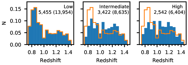
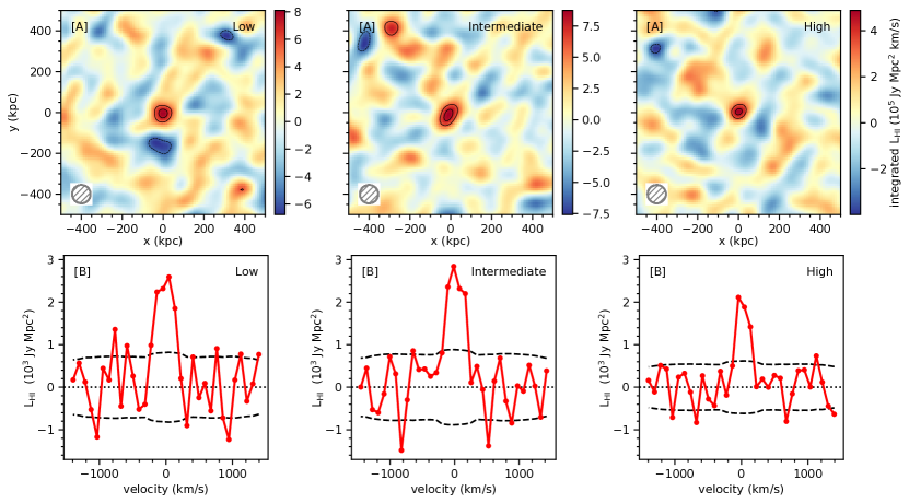
We divide our sample of 11,419 galaxies (28,993 Hi 21 cm subcubes) into three stellar-mass subsamples with (“Low”), (“Intermediate”), and (“High”)555 The stellar-mass ranges of the three subsamples were chosen such that a clear () detection of the stacked Hi 21 cm emission signal is obtained for each subsample. However, we emphasise that the conclusions of this Letter do not depend on the exact choice of the stellar-mass bins. The number of galaxies and Hi 21 cm subcubes in each subsample are provided in Table 1. The redshift distributions of the three stellar-mass subsamples are different (see Figure 1). We correct for this difference by assigning weights to each Hi 21 cm subcube such that the redshift distribution of each stellar-mass subsample is effectively identical. Specifically, the weights ensure that the effective redshift distributions of the intermediate- and high-stellar-mass subsamples are identical to that of the low-stellar-mass subsample; the mean redshift of the final redshift distribution is . We use these weights while computing all average quantities for the three stellar-mass subsamples.
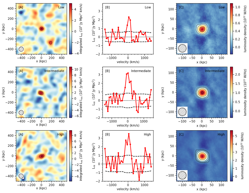
We separately stacked the Hi 21 cm emission and the rest-frame 1.4 GHz continuum emission of the galaxies in the three stellar-mass subsamples, following the procedures of Sections 2.2. Figure 2 shows the stacked Hi 21 cm emission images, the stacked Hi 21 cm spectra, and the stacked rest-frame 1.4 GHz continuum images of the three subsamples. We obtain clear detections of the average Hi 21 cm emission signal in all three cases, at statistical significance. We also detect the stacked rest-frame 1.4 GHz continuum emission at high significance () in all three subsamples. The average Hi masses and the average SFRs of galaxies in the three subsamples are listed in Table 1. We find that the average SFR and the average stellar mass of the galaxies in the three subsamples are in excellent agreement with the star-forming main sequence at (see Table 1; Whitaker et al., 2014; Chowdhury et al., 2022a).
| Low | Intermediate | High | |
| Stellar Mass Range () | |||
| Number of Hi 21 cm Subcubes | 13,954 | 8,635 | 6,404 |
| Number of Galaxies | 5,455 | 3,422 | 2,542 |
| Average Redshift | 1.01 | 1.01 | 1.01 |
| Average Stellar Mass () | |||
| Average Hi Mass () | |||
| Average SFR () | |||
| Main-sequence SFR () | 3.8 | 8.9 | 17.3 |
| Hi depletion timescale (Gyr) |
| Low | Intermediate | High | |
| Stellar Mass Range () | |||
| Average Stellar Mass () | |||
| Average Hi Mass () | |||
| Average SFR () | |||
| Hi depletion timescale (Gyr) | |||
We use the extended GALEX Arecibo SDSS survey (xGASS; Catinella et al., 2018) to compare our measurements of the Hi properties of star-forming galaxies at to those of galaxies in the local Universe. The xGASS Survey used the Arecibo telescope to measure the Hi masses of a stellar-mass-selected sample of galaxies with at . The stellar masses and SFRs of the xGASS galaxies used in this work were obtained from the publicly available catalogue of the “xGASS representative sample”. The stellar masses in this catalogue are from Kauffmann et al. (2003) and Brinchmann et al. (2004), while the SFRs were computed using a combination of Galex near-ultraviolet (NUV) and WISE mid-infrared (MIR) data or via spectral energy distribution fits for galaxies for which MIR data were not available (Catinella et al., 2018).
The main sample of the GMRT-CAT survey consists of blue, star-forming galaxies at . In order to ensure a fair comparison between the Hi properties of the GMRT-CAT galaxies and those of the xGASS galaxies, we restrict to blue galaxies, with NUVr, in the xGASS sample. We divide the xGASS galaxies into three stellar-mass subsamples, using the same “Low”, “Intermediate”, and “High” stellar-mass ranges as for the DEEP2 galaxies. Further, for each xGASS subsample, we use weights to ensure that the stellar-mass distribution within the subsample is effectively identical to that of the corresponding (Low, Intermediate, or High) subsample at . In passing, we note that the average Hi mass of xGASS galaxies in the three stellar-mass subsamples obtained using a cut in the SFR- plane to select main-sequence galaxies is consistent with the values obtained by selecting blue galaxies with NUVr.
The average Hi masses of the blue xGASS galaxies in the three stellar-mass sub-samples are listed in Table 2; the errors on the averages were computed using bootstrap resampling with replacement. The table also lists, for comparison, the GMRT-CAT1 measurements of the average Hi masses of blue galaxies in the same stellar-mass subsamples at . We find that, across the stellar-mass range , the average Hi mass of the galaxies is higher than that of local Universe galaxies, by a factor of .
We determined the relation at by fitting a power-law relation to our measurements of the average Hi mass of blue star-forming galaxies in the three stellar-mass subsamples at , following the procedures in Appendix A. We find that the relation for main-sequence galaxies at is
| (1) |
where . In order to compare the relation of blue star-forming galaxies at to that of blue star-forming galaxies at , we also fitted a power-law relation, using the procedures of Appendix A, to the measurements of in blue xGASS galaxies in the three stellar-mass subsamples of Table 2, with stellar-mass distributions identical to those of the subsamples of galaxies at . We find that the best-fit relation for blue galaxies at is .666We note that the relation for blue xGASS galaxies obtained by fitting to the values in the three stellar-mass subsamples is consistent with that obtained by fitting to values in small bins, separated by 0.1 dex.
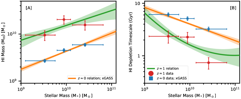
Figure 3[A] shows the relations for blue star-forming galaxies at and . We find no statistically significant evidence for an evolution in the slope of the relation from to . However, we find clear evidence that the relation has shifted downwards from to . Specifically, our measurements show that the relation of blue star-forming galaxies at lies a factor of above the local Universe relation.
In passing, we emphasize that the relations of this Letter, at both and , were obtained by fitting a relation to measurements of in three stellar-mass subsamples. This approach is different from that typically followed for galaxies at , where the relation is obtained by fitting to estimates of in multiple stellar-mass subsamples (e.g. Saintonge & Catinella, 2022). The difference arises from the fact that the averaging in a stacking analysis is carried out on the Hi masses themselves, rather than on the logarithm of the Hi masses; in general, the logarithm of the average value of a given quantity is not the same as the average of the individual logarithms (e.g. Brown et al., 2015). Care must hence be taken when comparing scaling relations obtained from simulations with those obtained from stacking analyses such as the present work, or when comparing the scaling relations from stacking analyses with those based on direct measurements of , and hence on estimates of . Specifically, the scaling relations obtained from the stacking analysis yield the mean Hi mass at a given stellar mass. Conversely, for a log-normal distribution of Hi masses, the scaling relations obtained from direct measurements yield the median HI mass at a given stellar mass. Further, again for a log-normal distribution of Hi masses with scatter , = . Assuming that the scatter of the scaling relation at is independent of and that it is equal to the scatter of dex measured at (Catinella et al., 2018), the “direct” relation would be offset downward from Equation 1 by 0.184 dex.
3.2 The Hi Depletion Timescale as a Function of Stellar Mass
The availability of cold gas regulates the star-formation activity in a galaxy. The Hi depletion timescale (), defined as the ratio of the Hi mass of the galaxy to its SFR, quantifies the approximate timescale for which the galaxy can sustain its current SFR, in the absence of accretion of fresh Hi from the CGM. In other words, accretion of gas from the CGM on a timescale of is required to sustain the current star-formation activity of the galaxy.
We define the “characteristic” Hi depletion timescale of a sample of galaxies as . We combined the average SFRs of galaxies in the three subsamples with their average Hi masses to estimate the characteristic Hi depletion timescale, , of galaxies at , as a function of their average stellar masses. Table 1 lists the values of the galaxies in the three stellar-mass subsamples at , while the estimates of are plotted against the average stellar mass in Figure 3[B]. For comparison, the figure also shows the characteristic Hi depletion timescale of the xGASS galaxies in the same three stellar-mass subsamples, while Table 2 compares the values of for the galaxies at and . We find that the characteristic Hi depletion timescale of blue star-forming galaxies at is times lower than that of similar galaxies with the same stellar mass distribution at .
In passing, we note that the “characteristic” Hi depletion timescale, , for a sample of galaxies may be different from the average of the depletion timescales of the individual galaxies, . Indeed, for the xGASS galaxies, we find that the values in the three stellar-mass subsamples are higher than the corresponding values by factors of . However, this does not affect the results of this Letter because we consistently compare the characteristic depletion timescales of the different galaxy subsamples, at both and .
We obtained the relation at by combining our estimate of the relation at (Equation 1) with a relation for the star-forming main sequence at from Whitaker et al. (2014). These authors provide best-fitting relations to the star-forming main sequence for the redshift ranges and ; we interpolated the best-fit parameters between the two redshift intervals to find that the main-sequence relation at is . Combining this relation with the relation of Equation 1, we find that the relation for main-sequence galaxies at is777We note that the uncertainties on the relation of Equation 2 are dominated by the uncertainties on the relation at , with relatively little contribution from the uncertainties in the main-sequence relation of Whitaker et al. (2014). The errors on the parameters in Equation 2 were hence obtained by ignoring the uncertainties in the main-sequence relation.:
| (2) |
We emphasise that Equation 2 was not obtained by fitting a relation to our measurements of the characteristic Hi depletion timescale in the three subsamples. However, Figure 3[B] shows that our measurements of in the three subsamples are consistent with the relation of Equation 2.
Overall, we find that blue star-forming galaxies at , with stellar masses in the range have larger Hi reservoirs than those of blue galaxies at , by a factor of . However, the evolution of the star-forming main-sequence by a factor of from to (e.g. Whitaker et al., 2014) implies that the characteristic Hi depletion timescales of blue star-forming galaxies at are lower, by factors of , than those of local galaxies. The results of this Letter thus extend the findings of the earlier GMRT Hi 21 cm stacking studies (Chowdhury et al., 2020, 2021, 2022a, 2022b) that blue star-forming galaxies at have a large average Hi mass but a short characteristic Hi depletion timescale to the entire stellar mass range .
3.3 The Hi Fraction as a Function of the Specific SFR
The Hi fractions () of galaxies in the local Universe and their specific SFRs () are known to be correlated, with a scatter of dex (Catinella et al., 2018); this is one of the tightest atomic gas scaling relations at (Catinella et al., 2018). The locations of galaxies in the sSFR plane are indicative of the efficiency with which their Hi is being converted to stars. In this section, we investigate the redshift evolution of the relation between and sSFR, for blue star-forming galaxies, from to .
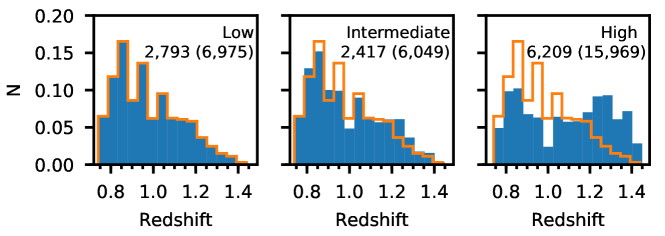
We divide our sample of 11,419 galaxies into three sSFR subsamples with sSFR (“Low”), sSFR (“Intermediate”), and sSFR (“High”)888 The sSFR ranges of the three subsamples were chosen such that a clear () detection of the stacked Hi 21 cm emission signal is obtained for each subsample. However, we emphasise that the conclusions of this section do not depend on the exact choice of the sSFR bins.. The numbers of galaxies and Hi 21 cm subcubes in each subsample are listed in Table 3, while the redshift distributions of the three sSFR subsamples are shown in Figure 4. The high-sSFR subsample contains a significantly larger number of galaxies at higher redshifts than the other two subsamples; this is primarily due to the redshift evolution of the star-forming main sequence within our redshift coverage, (e.g. Whitaker et al., 2014). We corrected for this difference in the redshift distributions of the subsamples by using weights such that the effective redshift distributions of the intermediate- and high-sSFR subsamples are identical to that of the low-sSFR subsample. We separately stacked the Hi 21 cm subcubes of the galaxies in the three subsamples, following the procedures of Section 2.2, using the above weights to ensure that the redshift distributions of the three subsamples are identical.
Figure 3 shows the stacked Hi 21 cm emission images and the stacked Hi 21 cm spectra of galaxies in the three sSFR subsamples. We obtain clear detections, with statistical significance, of the average Hi 21 cm emission signals from galaxies in the three subsamples. The average Hi mass and the “characteristic” Hi fraction, , of the galaxies in each subsample are listed in Table 3.
| Low | Intermediate | High | |
| sSFR Range () | |||
| Number of Hi 21 cm Subcubes | 6,975 | 6,049 | 15,969 |
| Number of Galaxies | 2,793 | 2,417 | 6,209 |
| Average Redshift | 0.97 | 0.97 | 0.97 |
| Average sSFR () | |||
| Average Stellar Mass () | |||
| Average Hi Mass () | |||
| Characteristic Hi Fraction |
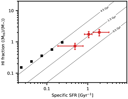
Our measurements of the characteristic Hi fraction of star-forming galaxies in the three sSFR subsamples at are shown in Figure 6; also shown for comparison are the characteristic Hi fractions of blue xGASS galaxies at (Catinella et al., 2018). Note that the average sSFR of the DEEP2 galaxies in the low-sSFR subsample is , while there are only 3 galaxies in the xGASS survey with sSFR . This is because the main sequence evolves between and , with the sSFR of galaxies at a fixed stellar mass being times higher at than at (e.g. Whitaker et al., 2014).
The straight lines in Figure 6 are the loci of constant depletion timescales on the plane. The characteristic Hi depletion timescale of main-sequence galaxies in the local Universe is Gyr, with a large scatter around the mean (Saintonge et al., 2017). Figure 6 shows that the characteristic Hi fractions and the average sSFRs of blue xGASS galaxies at are consistent with the Gyr line. However, it is clear from Figure 6 that star-forming galaxies at do not follow the sSFR relation of local Universe galaxies. This is consistent with our earlier results (e.g. Chowdhury et al., 2020, 2021) that blue star-forming galaxies at have a low characteristic Hi depletion timescale of Gyr. This evolution of the sSFR relation from to is different from the behaviour of the molecular component: the molecular gas depletion timescales in main-sequence galaxies are typically Gyr at , with no significant evidence for redshift evolution over (e.g. Saintonge et al., 2017; Genzel et al., 2015).
The short Hi depletion timescale of galaxies at (or, equivalently, the high Hi star-forming efficiency) is indicative of a very efficient conversion of Hi to , which then directly fuels the high star-formation activity. The difference between local Universe galaxies (with massive Hi reservoirs but low star-forming efficiency) and star-forming galaxies at may lie in the typical Hi surface densities in the galaxies; a high Hi surface density is likely to be a requirement for efficient conversion of Hi to (e.g. Leroy et al., 2008). In other words, it appears that the efficiency of conversion of Hi to stars is different at , towards the end of the epoch of peak star-formation activity in the Universe, from that at , with the Hi in galaxies at being able to fuel star-formation far more efficiently than at . Measurements of the average Hi surface density profiles of the GMRT-CAT galaxies would allow one to test this hypothesis.
4 Summary
In this Letter, we report the first determinations of Hi scaling relations of galaxies at , measuring the Hi properties of blue star-forming galaxies at as a function of stellar mass and sSFR, based on data from the GMRT-CAT1 survey. We divided our main sample of 11,419 blue star-forming galaxies at into three stellar-mass subsamples and detected the stacked Hi 21 cm emission signals from all three subsamples at significance. We fitted a power-law relation for the dependence of the average Hi mass on the average stellar mass, to obtain . We compared the relation at to that for blue galaxies at to find that the slope of the relation at is consistent with that at . However, we find that the relation at has shifted upwards from the relation at , by a factor of . We combined our measurements of the average Hi mass in the three stellar-mass subsamples with measurements of their average SFRs, obtained by stacking the rest-frame 1.4 GHz continuum emission, to obtain the characteristic Hi depletion timescale, , of the three subsamples. We find that the characteristic Hi depletion timescale of blue star-forming galaxies at , over the stellar mass range , is times lower than that at , for blue galaxies with similar stellar masses. We also divided the galaxies into three sSFR subsamples, obtaining detections of the stacked Hi 21 cm emission signals in all three subsamples, at significance. We find that the sSFR relation shows evidence for redshift evolution, with galaxies at having a lower characteristic Hi fraction, by a factor of , than what is expected from the extrapolation of the relation at to higher sSFR values. We thus find that star-forming galaxies at are able to convert their Hi reservoirs into stars with much higher efficiency than galaxies at . This is unlike the situation for molecular gas, where the efficiency of conversion of molecular gas to stars in main-sequence galaxies shows no significant evolution over .
References
- Astropy Collaboration et al. (2013) Astropy Collaboration, Robitaille, T. P., Tollerud, E. J., et al. 2013, A&A, 558, A33, doi: 10.1051/0004-6361/201322068
- Bera et al. (2019) Bera, A., Kanekar, N., Chengalur, J. N., & Bagla, J. S. 2019, ApJ, 882, L7, doi: 10.3847/2041-8213/ab3656
- Blyth et al. (2016) Blyth, S., Baker, A. J., Holwerda, B., et al. 2016, in MeerKAT Science: On the Pathway to the SKA, 4
- Brinchmann et al. (2004) Brinchmann, J., Charlot, S., White, S. D. M., et al. 2004, MNRAS, 351, 1151, doi: 10.1111/j.1365-2966.2004.07881.x
- Brown et al. (2015) Brown, T., Catinella, B., Cortese, L., et al. 2015, MNRAS, 452, 2479, doi: 10.1093/mnras/stv1311
- Catinella & Cortese (2015) Catinella, B., & Cortese, L. 2015, MNRAS, 446, 3526, doi: 10.1093/mnras/stu2241
- Catinella et al. (2018) Catinella, B., Saintonge, A., Janowiecki, S., et al. 2018, MNRAS, 476, 875, doi: 10.1093/mnras/sty089
- Chengalur et al. (2001) Chengalur, J. N., Braun, R., & Wieringa, M. 2001, A&A, 372, 768, doi: 10.1051/0004-6361:20010547
- Chowdhury et al. (2022a) Chowdhury, A., Kanekar, N., & Chengalur, J. N. 2022a, ApJ, 931, L34, doi: 10.3847/2041-8213/ac6de7
- Chowdhury et al. (2022b) —. 2022b, ApJ, 937, 103. https://arxiv.org/abs/2207.00031
- Chowdhury et al. (2022c) —. 2022c, ApJ, 935, L5, doi: 10.3847/2041-8213/ac8150
- Chowdhury et al. (2020) Chowdhury, A., Kanekar, N., Chengalur, J. N., Sethi, S., & Dwarakanath, K. S. 2020, Nature, 586, 369, doi: 10.1038/s41586-020-2794-7
- Chowdhury et al. (2021) Chowdhury, A., Kanekar, N., Das, B., Sethi, S., & Dwarakanath, K. S. 2021, ApJ, Submitted
- Condon (1992) Condon, J. J. 1992, ARA&A, 30, 575, doi: 10.1146/annurev.aa.30.090192.003043
- Condon et al. (2002) Condon, J. J., Cotton, W. D., & Broderick, J. J. 2002, AJ, 124, 675, doi: 10.1086/341650
- Davé et al. (2019) Davé, R., Anglés-Alcázar, D., Narayanan, D., et al. 2019, MNRAS, 486, 2827, doi: 10.1093/mnras/stz937
- Davé et al. (2020) Davé, R., Crain, R. A., Stevens, A. R. H., et al. 2020, MNRAS, 497, 146, doi: 10.1093/mnras/staa1894
- Delhaize et al. (2013) Delhaize, J., Meyer, M. J., Staveley-Smith, L., & Boyle, B. J. 2013, MNRAS, 433, 1398, doi: 10.1093/mnras/stt810
- Diemer et al. (2018) Diemer, B., Stevens, A. R. H., Forbes, J. C., et al. 2018, ApJS, 238, 33, doi: 10.3847/1538-4365/aae387
- Fabello et al. (2011) Fabello, S., Catinella, B., Giovanelli, R., et al. 2011, MNRAS, 411, 993, doi: 10.1111/j.1365-2966.2010.17742.x
- Fernández et al. (2016) Fernández, X., Gim, H. B., van Gorkom, J. H., et al. 2016, ApJ, 824, L1, doi: 10.3847/2041-8205/824/1/L1
- Genzel et al. (2015) Genzel, R., Tacconi, L. J., Lutz, D., et al. 2015, ApJ, 800, 20, doi: 10.1088/0004-637X/800/1/20
- Gogate et al. (2020) Gogate, A. R., Verheijen, M. A. W., Deshev, B. Z., et al. 2020, MNRAS, 496, 3531, doi: 10.1093/mnras/staa1680
- Guo et al. (2021) Guo, H., Jones, M. G., Wang, J., & Lin, L. 2021, ApJ, 918, 53, doi: 10.3847/1538-4357/ac062e
- Jaffé et al. (2013) Jaffé, Y. L., Poggianti, B. M., Verheijen, M. A. W., Deshev, B. Z., & van Gorkom, J. H. 2013, MNRAS, 431, 2111, doi: 10.1093/mnras/stt250
- Kanekar et al. (2016) Kanekar, N., Sethi, S., & Dwarakanath, K. S. 2016, ApJ, 818, L28, doi: 10.3847/2041-8205/818/2/L28
- Kauffmann et al. (2003) Kauffmann, G., Heckman, T. M., White, S. D. M., et al. 2003, MNRAS, 341, 33, doi: 10.1046/j.1365-8711.2003.06291.x
- Lagos et al. (2018) Lagos, C. d. P., Tobar, R. J., Robotham, A. S. G., et al. 2018, MNRAS, 481, 3573, doi: 10.1093/mnras/sty2440
- Lah et al. (2007) Lah, P., Chengalur, J. N., Briggs, F. H., et al. 2007, MNRAS, 376, 1357, doi: 10.1111/j.1365-2966.2007.11540.x
- Leroy et al. (2008) Leroy, A. K., Walter, F., Brinks, E., et al. 2008, AJ, 136, 2782, doi: 10.1088/0004-6256/136/6/2782
- Madau & Dickinson (2014) Madau, P., & Dickinson, M. 2014, ARA&A, 52, 415, doi: 10.1146/annurev-astro-081811-125615
- Mostek et al. (2012) Mostek, N., Coil, A. L., Moustakas, J., Salim, S., & Weiner, B. J. 2012, ApJ, 746, 124, doi: 10.1088/0004-637X/746/2/124
- Newman et al. (2013) Newman, J. A., Cooper, M. C., Davis, M., et al. 2013, ApJS, 208, 5, doi: 10.1088/0067-0049/208/1/5
- Rhee et al. (2016) Rhee, J., Lah, P., Chengalur, J. N., Briggs, F. H., & Colless, M. 2016, MNRAS, 460, 2675, doi: 10.1093/mnras/stw1097
- Saintonge & Catinella (2022) Saintonge, A., & Catinella, B. 2022, ARA&A, 60, 319, doi: 10.1146/annurev-astro-021022-043545
- Saintonge et al. (2017) Saintonge, A., Catinella, B., Tacconi, L. J., et al. 2017, ApJS, 233, 22, doi: 10.3847/1538-4365/aa97e0
- Salim et al. (2009) Salim, S., Dickinson, M., Michael Rich, R., et al. 2009, ApJ, 700, 161, doi: 10.1088/0004-637X/700/1/161
- Sinigaglia et al. (2022) Sinigaglia, F., Rodighiero, G., Elson, E., et al. 2022, arXiv e-prints, arXiv:2208.01121. https://arxiv.org/abs/2208.01121
- Tacconi et al. (2020) Tacconi, L. J., Genzel, R., & Sternberg, A. 2020, ARA&A, 58, 157, doi: 10.1146/annurev-astro-082812-141034
- Virtanen et al. (2020) Virtanen, P., Gommers, R., Oliphant, T. E., et al. 2020, Nature Methods, 17, 261, doi: 10.1038/s41592-019-0686-2
- Weiner et al. (2009) Weiner, B. J., Coil, A. L., Prochaska, J. X., et al. 2009, ApJ, 692, 187, doi: 10.1088/0004-637X/692/1/187
- Whitaker et al. (2012) Whitaker, K. E., van Dokkum, P. G., Brammer, G., & Franx, M. 2012, ApJ, 754, L29, doi: 10.1088/2041-8205/754/2/L29
- Whitaker et al. (2014) Whitaker, K. E., Franx, M., Leja, J., et al. 2014, ApJ, 795, 104, doi: 10.1088/0004-637X/795/2/104
- White et al. (2007) White, R. L., Helfand, D. J., Becker, R. H., Glikman, E., & de Vries, W. 2007, ApJ, 654, 99, doi: 10.1086/507700
- Willmer et al. (2006) Willmer, C. N. A., Faber, S. M., Koo, D. C., et al. 2006, ApJ, 647, 853, doi: 10.1086/505455
- Yun et al. (2001) Yun, M. S., Reddy, N. A., & Condon, J. J. 2001, ApJ, 554, 803, doi: 10.1086/323145
- Zwaan (2000) Zwaan, M. A. 2000, PhD thesis, Ph.D. Thesis, Groningen: Rijksuniversiteit, 2000
Appendix A Fitting Power-law Relations to Stacked Measurements
We fitted a power-law relation of the form in Equation A1 to our measurements of the average Hi mass in the three stellar-mass subsamples to determine the dependence of the Hi mass of star-forming galaxies at on their stellar mass.
| (A1) |
The fitting was done via a minimization, taking into account the stellar-mass distribution of the galaxies in each of the three subsamples. Specifically, for given trial values of and , we use the stellar masses of the 11,419 galaxies of our sample in Equation A1 to estimate their individual Hi masses, . Next, we use these individual Hi masses to compute the weighted-average Hi mass of the ’th subsample, , with the weights being the same as those used to stack the Hi 21 cm emission signals of the subsample. Through this procedure, we effectively obtain the average Hi masses of the three subsamples as a function of and , assuming that the relation at can be described by Equation A1. The parameters and are finally obtained by minimising, using a standard steepest-descent approach999The optimization was carried out using an implementation of the Levenberg-Marquardt algorithm in the scipy package (Virtanen et al., 2020)., the given by
| (A2) |
In the above equation, and are the measurement of the average Hi mass in the ’th subsample and the uncertainty on the measurement, respectively.