Optimizing Learning Rate Schedules
for Iterative Pruning of Deep Neural Networks

Abstract

The importance of learning rate (LR) schedules on network pruning has been observed in a few recent works. As an example, Frankle and Carbin (2019) highlighted that winning tickets (i.e., accuracy preserving subnetworks) can not be found without applying a LR warmup schedule and Renda, Frankle and Carbin (2020) demonstrated that rewinding the LR to its initial state at the end of each pruning cycle improves performance. In this paper, we go one step further by first providing a theoretical justification for the surprising effect of LR schedules. Next, we propose a LR schedule for network pruning called SILO, which stands for S-shaped Improved Learning rate Optimization. The advantages of SILO over existing state-of-the-art (SOTA) LR schedules are two-fold: (i) SILO has a strong theoretical motivation and dynamically adjusts the LR during pruning to improve generalization. Specifically, SILO increases the LR upper bound (max_lr) in an S-shape. This leads to an improvement of 2% - 4% in extensive experiments with various types of networks (e.g., Vision Transformers, ResNet) on popular datasets such as ImageNet, CIFAR-10/100. (ii) In addition to the strong theoretical motivation, SILO is empirically optimal in the sense of matching an Oracle, which exhaustively searches for the optimal value of max_lr via grid search. We find that SILO is able to precisely adjust the value of max_lr to be within the Oracle optimized interval, resulting in performance competitive with the Oracle with significantly lower complexity.

1 Introduction

Network pruning is the process of simplifying neural networks by pruning weights, filters or neurons. (LeCun, Denker, and Solla 1990; Han et al. 2015). Several state-of-the-art pruning methods (Renda, Frankle, and Carbin 2019; Frankle and Carbin 2019) have demonstrated that a significant quantity of parameters can be removed without sacrificing accuracy. This greatly reduces the resource demand of neural networks, such as storage requirements and energy consumption (He et al. 2020; Wang, Li, and Wang 2021).

The inspiring performance of pruning methods hinges on a key factor - Learning Rate (LR). Specifically, (Frankle and Carbin 2019) proposed the Lottery Ticket Hypothesis and demonstrated that the winning tickets (i.e., the pruned network that can train in isolation to full accuracy) cannot be found without applying a LR warmup schedule. In a follow-up work, (Renda, Frankle, and Carbin 2019) proposed LR rewinding which rewinds the LR schedule to its initial state during iterative pruning and demonstrated that it can outperform standard fine-tuning. In summary, the results in both works suggest that, besides the pruning metric, LR also plays an important role in network pruning and could be another key to improving the pruning performance.

In this paper, we take existing studies one step further and aim to optimize the choice of LR for iterative network pruning. We explore a new perspective on adapting the LR schedule to improve the iterative pruning performance. Our contributions to network pruning are as follows.

1. Motivation and Theoretical Study. We explore the optimal choice of LR during pruning and find that the distribution of weight gradients tends to become narrower during pruning, suggesting that a larger value of LR should be used to retrain the pruned network. This finding is further verified by our theoretical development. More importantly, our theoretical results suggest that the optimal increasing trajectory of LR should follow an S-shape.

2. Proposed SILO. We propose a novel LR schedule for network pruning called SILO, which stands for S-Shaped Improved Learning rate Optimization. Motivated by our theoretical development, SILO precisely adjusts the LR by increasing the LR upper bound (max_lr) in an S-shape. We highlight that SILO is method agnostic and works well with numerous pruning methods.

3. Experiments. We compare SILO to four LR schedule benchmarks via both classical and state-of-the-art (SOTA) pruning methods. We observe that SILO outperforms LR schedule benchmarks, leading to an improvement of 2% - 4% in extensive experiments with SOTA networks (e.g., Vision Transformer (Dosovitskiy et al. 2020), ResNet (He et al. 2016) & VGG (Simonyan and Zisserman 2014)) on large-scale datasets such as ImageNet (Deng et al. 2009) and popular datasets such as CIFAR-10/100 (Krizhevsky et al. 2009).

4. Comparison to Oracle. We examine the optimality of SILO by comparing it to an Oracle which exhaustively searches for the optimal value of max_lr via grid search. We find that SILO is able to precisely adjust max_lr to be within the Oracle’s optimized max_lr interval at each pruning cycle, resulting in performance competitive with the Oracle, but with significantly lower complexity.

2 Background

2.1 Prior Works on Network Pruning

Network pruning is an established idea dating back to 1990 (LeCun, Denker, and Solla 1990). The motivation is that networks tend to be overparameterized and redundant weights can be removed with a negligible loss in accuracy (Arora, Cohen, and Hazan 2018; Allen-Zhu, Li, and Song 2019; Denil et al. 2013). Given a trained network, one pruning cycle consists of three steps as follows.

1. Prune the network according to certain heuristics.

2. Freeze pruned parameters as zero.

3. Retrain the pruned network to recover the accuracy.

Repeating the pruning cycle multiple times until the target sparsity or accuracy is met is known as iterative pruning. Doing so often results in better performance than one-shot pruning (i.e., perform only one pruning cycle) (Han et al. 2015; Frankle and Carbin 2019; Li et al. 2017). There are two types of network pruning - unstructured pruning and structured pruning - which will be discussed in detail below.

Unstructured Pruning removes individual weights according to certain heuristics such as magnitude (Han et al. 2015) or gradient (Hassibi and Stork 1993; Lee et al. 2019; Xiao, Wang, and Rajasekaran 2019; Theis et al. 2018). Examples are (LeCun, Denker, and Solla 1990), which performed pruning based on the Hessian Matrix, and (Theis et al. 2018), which used Fisher information to approximate the Hessian Matrix. Similarly, (Han et al. 2015) removed weights with the smallest magnitude and this approach was further incorporated with the three-stage iterative pruning pipeline in (Han, Mao, and Dally 2015).

Structured Pruning involves pruning weights in groups, neurons, channels or filters (Yang et al. 2019; Luo, Wu, and Lin 2017; Tan and Motani 2020; Wang et al. 2020b; Lin et al. 2020). Examples are (Hu et al. 2016), which removed neurons with high average zero output ratio, and (Li et al. 2017), which pruned neurons with the lowest absolute summation values of incoming weights. More recently, (Yu et al. 2018) proposed the neuron importance score propagation algorithm to evaluate the importance of network structures. (Molchanov et al. 2019) used Taylor expansions to approximate a filter’s contribution to the final loss and (Wang et al. 2020a) optimized the neural network architecture, pruning policy, and quantization policy together in a joint manner.

Other Works. In addition to works mentioned above, several other works also share some deeper insights in network pruning (Liu et al. 2019; Zhu and Gupta 2018; Liu, Simonyan, and Yang 2019; Wang et al. 2020c). For example, (Liu, Simonyan, and Yang 2019) demonstrated that training-from-scratch on the right sparse architecture yields better results than pruning from pre-trained models. Similarly, (Wang et al. 2020c) suggested that the fully-trained network could reduce the search space for the pruned structure. More recently, (Luo and Wu 2020) addressed the issue of pruning residual connections with limited data and (Ye et al. 2020) theoretically proved the existence of small subnetworks with lower loss than the unpruned network. One milestone paper (Frankle and Carbin 2019) pointed out that re-initializing with the original parameters (known as weight rewinding) plays an important role in pruning and helps to further prune the network with negligible loss in accuracy. Some follow-on works (Zhou et al. 2019; Renda, Frankle, and Carbin 2019; Malach et al. 2020) investigated this phenomenon more precisely and applied this method in other fields (e.g., transfer learning (Mehta 2019) and natural language processing (Yu et al. 2020)).

2.2 The Important Role of Learning Rate

Several recent works (Renda, Frankle, and Carbin 2019; Frankle and Carbin 2019) have noticed the important role of LR in network pruning. For example, Frankle and Carbin (Frankle and Carbin 2019) demonstrated that training VGG-19 (Simonyan and Zisserman 2014) with a LR warmup schedule (i.e., increase LR to 1e-1 and decrease it to 1e-3) and a constant LR of 1e-2 results in comparable accuracy for the unpruned network. However, as the network is iteratively pruned, the LR warmup schedule leads to a higher accuracy (see Fig.7 in (Frankle and Carbin 2019)). In a follow-up work, Renda, Frankle and Carbin (Renda, Frankle, and Carbin 2019) further investigated this phenomenon and proposed a retraining technique called LR rewinding which can always outperform the standard retraining technique called fine-tuning (Han et al. 2015). The difference is that fine-tuning trains the unpruned network with a LR warmup schedule, and retrains the pruned network with a constant LR (i.e., the final LR of the schedule) in subsequent pruning cycles (Liu et al. 2019). LR rewinding retrains the pruned network by rewinding the LR warmup schedule to its initial state, namely that LR rewinding uses the same schedule for every pruning cycle. As an example, they demonstrated that retraining the pruned ResNet-50 using LR rewinding yields higher accuracy than fine-tuning (see Figs.1 & 2 in (Renda, Frankle, and Carbin 2019)). In (Liu and et al 2021), the authors also suggest that when pruning happens during the training phase with a large LR, models can easily recover from pruning than using a smaller LR. Overall, The results in these works suggest that, besides the pruning metric, LR also plays an important role in network pruning and could be another key to improving network pruning.

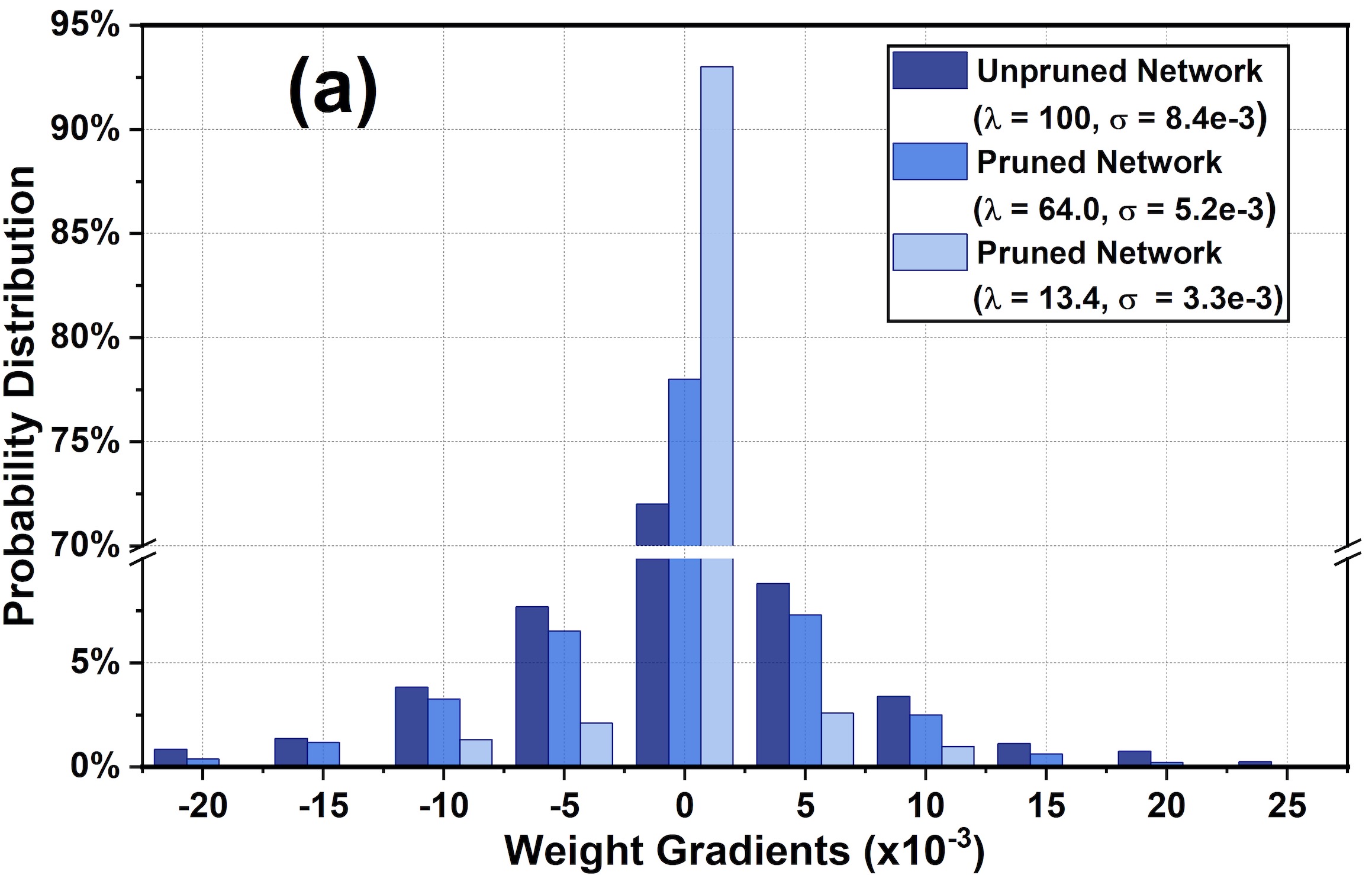
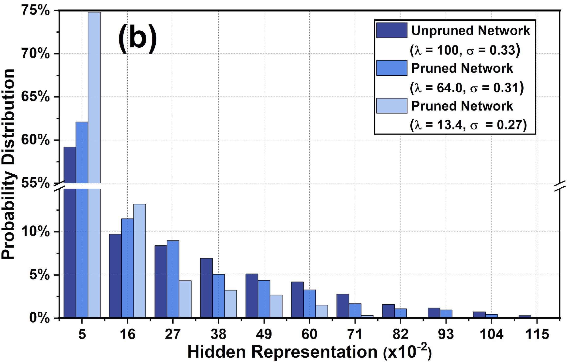
Figure 1: (a) The distribution of all weight gradients when iteratively pruning a fully connected ReLU network using global magnitude (i.e., prune weights with the lowest magnitude), where $\lambda$ is the percent of weights remaining and $\sigma$ is the standard deviation of the distribution. (b) The corresponding distribution of hidden representations. Please note that there is a line breaker in the vertical axis. Similar findings can be observed using popular networks and pruning methods (see Appendix).

Our work: In this paper, we explore a new perspective on adapting the LR schedule to improve the iterative pruning performance of ReLU-based networks. The proposed LR schedule is method agnostic and can work well with numerous pruning methods. We mainly focus on iterative pruning of ReLU-based networks for two reasons: (i) Iterative pruning tends to provide better pruning performance than one-shot pruning as reported in the literature (Frankle and Carbin 2019; Renda, Frankle, and Carbin 2019). (ii) ReLU has been widely used in many classical neural networks (e.g., ResNet, VGG, DenseNet) which have achieved outstanding performance in various tasks (e.g., image classification, object detection) (He et al. 2016; Simonyan and Zisserman 2014).

3 A New Insight on Network Pruning

In Section 3.1, we first provide a new insight in network pruning using experiments. Next, in Section 3.2, we provide a theoretical justification for our observed new insight and present some relevant theoretical results.

3.1 Weight Gradients during Iterative Pruning

(1) Experiment Setup. To exclude the influence of other factors, we start from a simple fully connected ReLU-based network with three hidden layers of 256 neurons each (results of other popular networks are summarized later). We train the network using the training dataset of CIFAR-10 via SGD (Ruder 2016) (momentum = 0.9 and a weight decay of 1e-4) with a batch size of 128 for 500 epochs. All hyperparameters are tuned for performance via grid search (e.g., LR from 1e-4 to 1e-2). We apply the global magnitude (Han et al. 2015) (i.e., remove weights with the smallest magnitude anywhere in the network) with a pruning rate of 0.2 (i.e., prune 20% of the remaining parameters) to iteratively prune the network for 10 pruning cycles and plot the distribution of all weight gradients when the network converges in Fig. 1(a), where $\lambda$ is the percent of weights remaining. In Fig. 1(a), there are 10 visible bins estimated by the Sturges’ Rule (Scott 2009) and each bin consists of three values (i.e., the probability distribution of networks). The edge values range from -0.022 to 0.027 with a bin width of 0.004.

(2) Experiment Results. In Fig. 1(a), we observe that the distribution of weight gradients tends to become narrower, i.e., the standard deviation of weight gradients $\sigma$ reduces from 8.4e-3 to 3.3e-3 when the network is iteratively pruned to $\lambda=13.4$. As an example, the unpruned network ($\lambda$ = 100) has more than 7% of weight gradients with values greater than 0.008 (rightmost 4 bars) or less than -0.012 (leftmost 2 bars), while the pruned network ($\lambda=13.4$) has less than 1% of weight gradients falling into those regions. It suggests that the magnitude of weight gradients tends to decrease as the network is iteratively pruned.

(3) New Insight. During the backpropagation, the weight update of $w_{i}$ is $w_{i}\leftarrow w_{i}+\alpha\frac{\partial\mathcal{L}}{\partial w_{i}}$, where $\alpha$ is the LR and $\mathcal{L}$ is the loss function. Assume that $\alpha$ is well-tuned to ensure the weight update (i.e., $\alpha\frac{\partial\mathcal{L}}{\partial w_{i}}$) is sufficiently large to prevent the network from getting stuck in local optimal points (Bengio 2012; Goodfellow, Bengio, and Courville 2016). As shown in Fig. 1(a), the magnitude of the weight gradient (i.e., $\frac{\partial\mathcal{L}}{\partial w_{i}}$) tends to decrease as the network is iteratively pruned. To preserve the same weight updating size and effect as before, a gradually larger value of LR ($\alpha$) should be used to retrain the pruned network during iterative pruning.

(4) Result Analysis. We now provide an explanation for the change in the distribution of weight gradients. We assume each $x_{i}w_{i}$ (i.e., $x_{i}\in\mathbb{R}$ is the neuron input and $w_{i}\in\mathbb{R}$ is the associated weight) is an i.i.d. random variable. Then, the variance of the neuron’s pre-activation output ($\sum_{i=1}^{n}x_{i}w_{i}$, $n$ is the number of inputs) will be $\sum_{i=1}^{n}\text{Var}(x_{i}w_{i})$. Pruning the network is equivalent to reducing the number of inputs from $n$ to $n-k$. This results in a smaller variance of $\sum_{i=1}^{n-k}\text{Var}(x_{i}w_{i})$, leading to a smaller standard deviation. Hence, the distribution of the pre-activation output after pruning is narrower. Since ReLU returns its raw input if the input is non-negative, the distribution of hidden representations (output of hidden layers) becomes narrower as well. This can be verified from Fig. 1(b), where we plot the distribution of hidden representations from the previous experiment. The key is that the weight gradient $\frac{\partial\mathcal{L}}{\partial w_{i}}$ is proportional to the hidden representation $x_{i}$ that associates with $w_{i}$ (i.e., $\frac{\partial\mathcal{L}}{\partial w_{i}}\propto x_{i}$). As the network is iteratively pruned, the distribution of hidden representations becomes narrower, leading to a narrower distribution of weight gradients. As a result, a larger LR should be used to retrain the pruned network.

(5) More Generalized Results. (i) Effect of Batch Normalization (BN) (Ioffe and Szegedy 2015): BN is a popular technique to reformat the distribution of hidden representations, so as to address the issue of internal covariate shift. We note that similar performance trends can be observed after applying BN as well (see Fig. 3 in the Appendix). (ii) Popular CNN Networks and Pruning Methods: In addition to the global magnitude used before, two unstructured pruning methods (i.e., layer magnitude, global gradient) suggested by (Blalock et al. 2020) and one structured pruning method (L1 norm pruning) (Li et al. 2017) are examined as well. Those methods are used to iteratively prune AlexNet (Krizhevsky and Hinton 2010), ResNet-20 and VGG-19 using CIFAR-10. The results using these popular neural networks largely mirror those in Figs. 1(a) & (b) as well. We refer the interested reader to Figs. 4 - 6 in the Appendix.

3.2 Theoretical Study and Motivation

In this subsection, we theoretically investigate how network pruning can influence the value of the desired LR. The proofs of the results given here are provided in the Appendix. First, we present some definitions.

Definition 1.

Average Activation Energy ($E_{AA}$): Given a network with fixed weights, input $X$ from a distribution $P$, and a layer $H=\{h_{1}(X),...,h_{N}(X)\}$ with $N$ nodes where $h_{i}(X)$ represents the function at the $i^{th}$ node. Then $E_{AA}(H)=\mathop{\mathbb{E}}_{X}[\frac{1}{N}\sum_{i}h_{i}(X)^{2}]$. This quantity reflects the average strength of the layer’s activations.

Definition 2.

Weight-Gradient Energy ($E_{WG}$): Let $W=[w_{1},...,w_{k}]$ and $W^{\prime}=[w^{\prime}_{1},...,w^{\prime}_{k}]$ represent the flattened weight vector before and after one epoch of training. Then $E_{WG}$ is the average change in weight magnitude before and after a single epoch of training (for the active unpruned weights), i.e., $E_{WG}(W,W^{\prime})=\mathbb{E}_{i}[(w_{i}-w^{\prime}_{i})^{2}]$. This measure quantifies how much the weights change after a single epoch of training.

We now demonstrate the impact of network pruning on the average activation energy of hidden layers.

Theorem 1.

Consider a ReLU activated neural network represented as $X\xrightarrow[]{W_{1}}H\xrightarrow[]{W_{2}}Y$, where $X\in\mathbb{R}^{d}$ is the input, $H=\{H_{1}(X),H_{2}(X),...,H_{N}(X)\}$ is of infinite width ($N=\infty$), and $Y$ is the network output. $W_{1}$ and $W_{2}$ represent network parameters (weights, biases). Furthermore, let $X\sim\mathcal{N}(0,\sigma_{\scaleto{X}{3pt}}^{2}I)$ and $W_{1}\sim\mathcal{N}(0,\sigma_{\scaleto{W}{3pt}}^{2}I)$, where $I$ is the identity matrix and $\sigma_{\scaleto{X}{3pt}},\sigma_{\scaleto{W}{3pt}}$ are scalars. Now, let us consider an iterative pruning method, where in each iteration a fraction $0\leq p\leq 1$ of the smallest magnitude weights are pruned (layer-wise pruning). Then, after $k$ iterations of pruning, it holds that

$$\begin{split}&4E_{AA}(H)\geq\sigma_{W}^{2}+d\sigma_{X}^{2}\sigma_{W}^{2}\Big{(}(1-p)^{k}+\\ &\hskip 5.69054pt\sqrt{\frac{4}{\pi}}\operatorname{erf^{-1}}\Big{(}1-(1-p)^{k}\Big{)}e^{-\left(\operatorname{erf^{-1}}\left(1-(1-p)^{k}\right)\right)^{2}}\Big{)}\end{split}$$ (1)

where $\operatorname{erf^{-1}}(.)$ is the inverse error function.

Next, using the above result, the following theorem establishes how the weight-gradient energy depends on the LR of the network, and the pruning iteration.

Theorem 2.

In Theorem 1’s setting, we consider a single epoch of weight update for the network across a training dataset $S=\{(X_{1},Y_{1}),..,(X_{n},Y_{n})\}$ using the cross-entropy loss, where $Y_{i}\in\{0,1\}$. Let $\alpha$ denote the learning rate. Let us denote the R.H.S of (1) by $C(\sigma_{X},\sigma_{W},p,k)$. Let the final layer weights before and after one training epoch be $W_{2}$ and $W_{2}^{\prime}$ respectively. We have,

where $\mathcal{N}_{k}(0,\sigma_{\scaleto{W}{3pt}}^{2}I)$ represents a normal distribution $\mathcal{N}(0,\sigma_{\scaleto{W}{3pt}}^{2}I)$ initialization of $W_{2}$, followed by $k$ iterations of pruning, and $\gamma$ is a constant.

Remark 1.

(Pruning and LR) Theorems 1 and 2 together establish how the choice of LR influences the lower bound of weight-gradient energy. Theorem 1 shows that the lower bound of activation energy of the hidden layer decreases as the network is pruned, and as Theorem 2 shows, this also reduces the lower bound of weight-gradient energy per epoch. Thus, to counter this reduction, it is necessary to increase the learning rate $\alpha$ as the number of pruning cycles grows, in order to ensure that the R.H.S of (60) remains fixed.

Remark 2.

(S-shape of LR During Iterative Pruning) Theorem 2 implies that to maintain a fixed weight-gradient energy of $\mathop{{}\mathbb{E}}_{W_{2}\sim\mathcal{N}_{k}(0,\sigma_{\scaleto{W}{3pt}}^{2}I)}[E_{WG}(W_{2},W_{2}^{\prime})]=K$, we must have the learning rate $\alpha\leq(K/\gamma C(\sigma_{X},\sigma_{W},p,k))^{1/2}$. We plot the adapted $\alpha$ assuming equality and find that this resembles an S-shape trajectory during iterative pruning.

4 A New Learning Rate Schedule

In Section 4.1, we first review existing works on LR schedules and shortlist four benchmarks for comparison. Next, in Section 4.2, we introduce SILO and highlight the difference with existing works. Lastly, in Section 4.3, we detail the algorithm of the proposed SILO.

Figure 2: Illustration of SILO during pruning. The S-shape red line is motivated from Theorem 1.

4.1 LR Schedule Benchmarks

Learning rate is the most important hyperparameter in training neural networks (Goodfellow, Bengio, and Courville 2016). The LR schedule is to adjust the value of LR during training by a pre-defined schedule. Three common LR schedules are summarized as follows.

1. LR Decay starts with a large initial LR and linearly decays it by a certain factor after a pre-defined number of epochs. Several recent works (You et al. 2019; Ge et al. 2019; An et al. 2017) have demonstrated that decaying LR helps the neural network to converge better and avoids undesired oscillations in optimization.

2. LR Warmup is to increase the LR to a large value over certain epochs and then decreases the LR by a certain factor. It is a popular schedule used by many practitioners for transfer learning (He et al. 2019) and network pruning (Frankle and Carbin 2019; Frankle et al. 2020).

3. Cyclical LR (Smith 2017) varies the LR cyclically between a pre-defined lower and upper bound. It has been widely used in many tasks (You et al. 2019).

All the three LR schedules and constant LR will be used as benchmarks for comparison. We note that, in addition to LR schedules which vary LR by a pre-defined schedule, adaptive LR optimizers such as AdaDelta (Zeiler 2012) and Adam (Kingma and Ba 2014) provide heuristic based approaches to adaptively vary the step size of weight update based on observed statistics of the past gradients. All of them are sophisticated optimization algorithms and much work (Gandikota et al. 2021; Jentzen et al. 2021) has been done to investigate their mechanisms. In this paper, the performance of all benchmarks and SILO will be evaluated using SGD with momentum = 0.9 and a weight decay of 1e-4 (same as (Renda, Frankle, and Carbin 2019; Frankle and Carbin 2019)). The effect of those adaptive LR optimizers on SILO will be discussed in Section B.2 of the Appendix.

4.2 SILO Learning Rate Schedule

To ensure the pruned network is properly trained during iterative pruning, we propose an S-shaped Improved Learning rate Schedule, called SILO, for iterative pruning of networks. As illustrated in Fig. 2, the main idea of the proposed SILO is to apply the LR warmup schedule at every pruning cycle, with a gradual increase of the LR upper bound (i.e., max_lr) in an S-shape as the network is iteratively pruned. This LR warmup schedule is meant to be flexible and can change depending on different networks and datasets.

The S-shape in SILO is inspired by Theorem 2 (see Remark 2) and will be further verified by comparing to an Oracle. We divide the S-shape into four phases and provide the intuition behind each phase as follows.

1. Phase-1-No Growth, SILO does not increase max_lr until the pruning cycle q (see Fig. 2). It is because the unpruned network often contains a certain amount of weights with zero magnitude. Those parameters are likely to be pruned at the first few pruning cycles, and removing such weights has negligible effect on the distribution of weight gradients.

2. Phase-2-Slow Growth i@, the pruning algorithm has removed most zero magnitude weights and started pruning weights with small magnitude. Pruning such weights has a small effect on distribution of weight gradients. Hence, we slightly increase max_lr after pruning cycle q.

3. Phase-3-Fast Growth, SILO greatly increases max_lr. It is because the pruning algorithm now starts removing weights with large magnitude and the distribution of weight gradients becomes much narrower. This requires a much larger LR for meaningful weight updates.

4. Phase-4-Slow Growth ii@, the network is now heavily pruned and very few parameters left in the network. By using the same pruning rate, a very small portion of the weights will be pruned. This could cause a marginal effect on the distribution of weight gradients. Hence, SILO slightly increases max_lr.

We note that SILO is designed based on the assumption that existing pruning methods tend to prune weights with small magnitude. The key difference with existing LR schedules (e.g., Cyclical LR, LR warmup) is that SILO is adaptive and able to precisely increase the value of max_lr as the network is iteratively pruned, while existing LR schedules do not factor in the need to change max_lr during different pruning cycles.

Algorithm 1 Algorithm of the Proposed SILO

1:lower bound $\epsilon$, upper bound $\delta+\epsilon$, pruning rate p, number of pruning cycles L, number of training epochs t, S-shape control term $\beta$, delay term q.

2:for $\texttt{m}=0$ to L do

3:     if $\texttt{m}\leq\texttt{q}$ then

4:         $\texttt{max\_lr}=\epsilon$

5:     else

6:         $\texttt{max\_lr}=\frac{\delta}{1+(\frac{\gamma}{1-\gamma})^{-\beta}}+\epsilon$, $\gamma=1-(1-\texttt{p})^{m-\texttt{q}}$      

7:for $\texttt{i}=0$ to t do

8:     (1) linearly warmup the LR to max_lr

9:     (2) drop the value of LR by 10 at certain epochs

4.3 Implementation of SILO

As for the implementation of SILO, we designed a function to estimate the value of max_lr as shown below.

$$\texttt{max\_lr}=\frac{\delta}{1+(\frac{\gamma}{1-\gamma})^{-\beta}}+\epsilon,$$ (3)

where $\gamma=1-(1-\texttt{p})^{m-\texttt{q}}$ is the input of the function and max_lr is the output of the function. The parameter p is the pruning rate and m is the number of completed pruning cycles. The parameters $\beta$ and q are used to control the shape of the S curve. The larger the $\beta$, the later the curve enters the Fast Growth phase. The parameter q determines at which pruning cycle SILO enters the Slow Growth i@ phase. When $q=0$, the No Growth phase will be skipped and $\gamma$ will be the proportion of pruned weights at the current pruning cycle. The parameters $\epsilon$ and $\delta$ determine the value range of max_lr. As the network is iteratively pruned, $\gamma$ increases and max_lr increases from $\epsilon$ to $\epsilon+\delta$ accordingly. The details of the SILO algorithm are summarized in Algorithm 1.

Parameter Selection for SILO. Algorithm 1 requires several inputs for implementation. The value of $\epsilon$ can be tuned using the validation accuracy of the unpruned network while the value of $\delta$ can be tuned using the validation accuracy of the pruned network with targeted sparsity. The pruning rate p and pruning cycles L are chosen to meet the target sparsity. The number of training epochs t should be large enough to guarantee the network convergence. Let q = 1 and $\beta$ = 5 could be a good choice and yield promising results as we demonstrate in the Section of Performance Evaluation. Furthermore, based on our experience, the value of q and $\beta$ could be tuned in the range of [0, 3] and [3, 6], respectively.

Original Top-1 Test Accuracy = 91.7% ($\lambda$ = 100)
$\lambda$	32.8	26.2	8.59	5.72
constant LR	88.1$\pm$0.9	87.5$\pm$0.7	82.8$\pm$0.9	79.1$\pm$0.8
LR decay	89.8$\pm$0.4	89.0$\pm$0.7	83.9$\pm$0.6	79.8$\pm$0.7
cyclical LR	89.7$\pm$0.6	88.2$\pm$0.7	84.1$\pm$0.8	80.3$\pm$0.7
LR-warmup	90.3$\pm$0.4	89.8$\pm$0.6	85.9$\pm$0.9	81.2$\pm$1.1
SILO (Ours)	90.8$\pm$0.5	90.3$\pm$0.4	87.5$\pm$0.8	82.7$\pm$1.2

Table 1: Top-1 test accuracy ($\pm$ std) of pruning ResNet-20 on CIFAR-10 using global magnitude.

Original Top-1 Test Accuracy = 92.2% ($\lambda$ = 100)
$\lambda$	32.8	26.2	8.59	5.72
constant LR	88.8$\pm$0.6	87.4$\pm$0.7	82.2$\pm$1.4	73.7$\pm$1.3
LR decay	89.4$\pm$0.4	88.6$\pm$0.5	83.3$\pm$0.8	75.4$\pm$0.9
cyclical LR	89.8$\pm$0.5	89.1$\pm$0.6	83.7$\pm$1.0	75.7$\pm$1.2
LR-warmup	90.2$\pm$0.5	89.8$\pm$0.8	84.5$\pm$0.9	76.5$\pm$1.0
SILO (Ours)	90.6$\pm$0.6	90.3$\pm$0.6	86.1$\pm$0.8	78.5$\pm$1.0

Table 2: Top-1 test accuracy ($\pm$ std) of pruning VGG-19 on CIFAR-10 using global gradient.

5 Performance Evaluation

5.1 Experimental Setup

We demonstrate that SILO can work well with different pruning methods across a wide range of networks and datasets. The details for each experiment are as follows.

1. Pruning ResNet-20 (He et al. 2016) on CIFAR-10 via global magnitude (i.e., prune weights with the lowest magnitude anywhere in the networks).

2. Pruning VGG-19 (Simonyan and Zisserman 2014) on CIFAR-10 via global gradient (i.e., prune weights with the lowest magnitude of (weight $\times$ gradient) anywhere in the network).

3. Pruning DenseNet-40 (Huang et al. 2017) on the CIFAR-100 dataset using Layer-adaptive Magnitude-based Pruning (LAMP) (Lee et al. 2020).

4. Pruning MobileNetV2 (Sandler et al. 2018) on the CIFAR-100 dataset using Lookahead Pruning (LAP) (Park et al. 2020).

5. Pruning ResNet-50 on ImageNet (i.e., ImageNet-1000) (Deng et al. 2009) using Iterative Magnitude Pruning (IMP) (Frankle and Carbin 2019).

6. Pruning Vision Transformer (ViT-B-16) (Dosovitskiy et al. 2020) on CIFAR-10 using IMP.

In each experiment, we compare SILO (q = 1, $\beta$ =5) to constant LR and the three shortlisted LR schedules: (i) LR decay, (ii) cyclical LR and (iii) LR warmup. The details of each LR schedule are summarized in Table 12 in the Appendix.

(1) Methodology. We train the network using the training dataset via SGD with momentum = 0.9 and a weight decay of 1e-4 (same as (Renda, Frankle, and Carbin 2019; Frankle and Carbin 2019)). Next, we prune the trained network with a pruning rate of 0.2 (i.e., 20% of remaining weights are pruned) in 1 pruning cycle. We repeat 25 pruning cycles in 1 run and use early-stop top-1 test accuracy (i.e., the corresponding test accuracy when early stopping criteria for validation error is met) to evaluate the performance. The results are averaged over 5 runs and the corresponding standard deviation are summarized in Tables 1 - 6, where the results of pruning ResNet-20, VGG-19, DenseNet-40, MobileNetV2, ResNet-50 and Vision Transformer (ViT-B-16) are shown, respectively. Some additional details (e.g., training epochs) and results are given in Tables 13 - 18 in the Appendix.

(2) Parameters for SOTA LR Schedules. To ensure fair comparison against prior SOTA LR schedules, we utilize implementations reported in the literature. Specifically, the LR schedules (i.e., LR-warmup) from Table 1 - 5 are from (Frankle and Carbin 2019), (Frankle et al. 2020), (Zhao et al. 2019), (Chin et al. 2020) and (Renda, Frankle, and Carbin 2019), respectively. The LR schedule (i.e., cosine decay) in Table 6 is from (Dosovitskiy et al. 2020).

(3) Parameters for other LR schedules. For the other schedules without a single ”best” LR in the literature, we tune the value of LR for each of them via a grid search with a range from 1e-4 to 1e-1 using the validation accuracy. Other related parameters (e.g., step size) are also tuned in the same manner. Lastly, we highlight that all LR schedules used, including SILO, are rewound to the initial state at the beginning of each pruning cycle, which is the same as the LR rewinding in (Renda, Frankle, and Carbin 2019).

(4) Source Code & Devices: We use Tesla V100 devices for our experiments, and the source code (including random seeds) will be released at the camera-ready stage.

Original Top-1 Test Accuracy = 74.6% ($\lambda$ = 100)
$\lambda$	32.8	26.2	8.59	5.72
constant LR	70.3$\pm$0.8	68.1$\pm$0.7	60.8$\pm$1.1	59.1$\pm$1.2
LR decay	71.2$\pm$0.8	69.0$\pm$0.6	62.6$\pm$1.2	60.3$\pm$1.4
cyclical LR	70.9$\pm$0.6	69.4$\pm$0.6	63.0$\pm$1.1	60.8$\pm$1.3
LR-warmup	71.5$\pm$0.7	69.6$\pm$0.8	63.9$\pm$1.0	61.2$\pm$0.9
SILO (Ours)	72.4$\pm$0.7	70.8$\pm$0.8	65.7$\pm$1.2	63.7$\pm$1.0

Table 3: Top-1 test accuracy ($\pm$ std) of pruning DenseNet-40 on CIFAR-100 using LAMP (Lee et al. 2020).

Original Top-1 Test Accuracy = 73.7% ($\lambda$ = 100)
$\lambda$	32.8	26.2	8.59	5.72
constant LR	69.8$\pm$1.1	68.2$\pm$0.9	63.8$\pm$1.1	62.1$\pm$1.2
LR decay	70.9$\pm$1.0	69.4$\pm$0.6	65.1$\pm$0.8	64.0$\pm$1.1
cyclical LR	71.5$\pm$0.7	69.6$\pm$0.6	65.3$\pm$1.1	64.3$\pm$1.2
LR-warmup	72.1$\pm$0.8	70.5$\pm$0.9	66.2$\pm$1.1	64.8$\pm$1.5
SILO (Ours)	72.5$\pm$0.6	71.0$\pm$0.7	68.8$\pm$0.8	66.8$\pm$1.4

Table 4: Top-1 test accuracy ($\pm$ std) of pruning MobileNetV2 on CIFAR-100 using LAP (Lee et al. 2020).

Original Top-1 Test Accuracy = 77.0% ($\lambda$ = 100)
$\lambda$	32.8	26.2	8.59	5.72
constant LR	74.2$\pm$0.8	73.9$\pm$0.7	70.5$\pm$0.6	69.2$\pm$0.9
LR decay	75.6$\pm$0.5	75.1$\pm$0.5	72.7$\pm$0.8	70.5$\pm$0.6
cyclical LR	76.5$\pm$0.5	75.5$\pm$0.6	73.4$\pm$0.8	71.2$\pm$0.7
LR-warmup	76.6$\pm$0.2	75.8$\pm$0.3	73.8$\pm$0.5	71.5$\pm$0.4
SILO (Ours)	76.8$\pm$0.4	76.1$\pm$0.7	75.2$\pm$0.8	73.8$\pm$0.6

Table 5: Top-1 test accuracy ($\pm$ std) of pruning ResNet-50 on ImageNet using IMP (Frankle and Carbin 2019).

Original Top-1 Test Accuracy = 98.0% ($\lambda$ = 100)
$\lambda$	32.8	26.2	8.59	5.72
constant LR	96.4$\pm$0.5	96.0$\pm$0.7	83.0$\pm$0.9	80.1$\pm$0.8
cosine decay	97.2$\pm$0.2	96.5$\pm$0.6	84.1$\pm$1.0	81.6$\pm$1.1
cyclical LR	97.0$\pm$0.2	96.5$\pm$0.6	83.4$\pm$0.6	81.0$\pm$1.1
LR-warmup	97.3$\pm$0.6	96.8$\pm$0.7	84.4$\pm$0.8	82.1$\pm$0.9
SILO (Ours)	97.7$\pm$0.5	97.4$\pm$0.6	85.5$\pm$0.9	83.4$\pm$0.8

Table 6: Top-1 test accuracy ($\pm$ std) of pruning Vision Transformer on CIFAR-10 using IMP (Frankle and Carbin 2019).

5.2 Performance Comparison

(1) Reproducing SOTA results. By using the implementations reported in the literature, we have correctly reproduced SOTA results. For example, the benchmark results of LR warmup in our Tables 1 - 6 are comparable to Fig.11 and Fig.9 of (Blalock et al. 2020), Table.4 in (Liu et al. 2019), Fig.3 in (Chin et al. 2020), Fig. 10 in (Frankle et al. 2020), Table 5 in (Dosovitskiy et al. 2020), respectively.

(2) SILO outperforms SOTA results. The key innovation of SILO is that the LR precisely increases as the network is pruned, by increasing max_lr in an S-shape as $\lambda$ decreases. This results in a much higher accuracy than all LR schedule benchmarks studied. For example, in Table 1, the top-1 test accuracy of SILO is 1.8% higher than the best performing schedule (i.e., LR-warmup) at $\lambda$ = 5.72. SILO also obtains the best performance when using larger models in Table 2 (i.e., 2.6% higher at $\lambda$ = 5.72) and using more difficult datasets in Table 3 (i.e., 4.0% higher at $\lambda$ = 5.72).

(3) Performance on ImageNet. In Table 5, we show the performance of SILO using IMP (i.e., the lottery ticket hypothesis pruning method) via ResNet-50 on ImageNet (i.e., the ILSVRC version) which contains over 1.2 million images from 1000 different classes. We observe that SILO still outperforms the best performing LR schedule benchmark (LR-warmup) by 1.9% at $\lambda=8.59$. This improvement increases to 3.2% when $\lambda$ reduces to 5.72.

(4) Performance on SOTA networks (Vision Transformer). Several recent works (Liu et al. 2021; Yuan et al. 2021) demonstrated that transformer based networks tend to provide excellent performance in computer vision tasks (e.g., classification). We now examine the performance of SILO using Vision Transformer (i.e., ViT-B16 with a resolution of 384). We note that the ViT-B16 uses Gaussian Error Linear Units (GELU, GELU(x) = x$\Phi(x)$, where $\Phi(x)$ is the standard Gaussian cumulative distribution function) as the activation function. We note that both ReLU and GELU have the unbounded output, suggesting that SILO could be helpful for pruning GELU based models as well.

We repeat the same experiment setup as above and compare the performance of SILO to other LR schedules using ViT-B16 in Table 6. We observe that SILO is able to outperform the standard implementation (cosine decay, i.e., decay the learning rate via the cosine function) by 1.3% at $\lambda=8.59$ in top-1 test accuracy. This improvement increases to 1.6% when $\lambda$ reduces to 5.72.

$\lambda$	100	51.3	32.9	21.1	5.72
Oracle max_lr	4	4.6	9.0	9.8	10.2
Oracle interval	[3.6,4.2]	[4.2,5.4]	[8.0,9.6]	[9.2,10.4]	[9.8,10.6]
SILO max_lr	4	4.32	9.2	9.9	9.99

Table 7: Comparison between Oracle max_lr, Oracle interval (both obtained via grid search) and max_lr estimated by SILO when iteratively pruning VGG-19 on CIFAR-10. Note that all values in the table are in hundredths.

5.3 Comparing SILO to an Oracle

Our new insight suggests that, due to the change in distribution of hidden representations during iterative pruning, LR should be re-tuned at each pruning cycle. SILO provides a method to adjust the max_lr in an S-shape, which is backed up by a theoretical result (see Theorem 2). We now further examine the S-shape trajectory of SILO by comparing SILO’s estimated max_lr to an Oracle, which uses the same LR warmup structure as SILO but exhaustively searches for the optimal value of max_lr at each pruning cycle. The Oracle’s max_lr at the current pruning cycle is chosen by grid search ranging from 1e-4 to 1e-1 and the best performing value (i.e., determined by validation accuracy) is used to train the network. The results of max_lr determined this way when iteratively pruning a VGG-19 on CIFAR-10 using the global magnitude are detailed in Table 7 via two metrics:

1. Oracle max_lr: The value of max_lr that provides the best validation accuracy.

2. Oracle interval: The value range of max_lr which performs within 0.5% of the best validation accuracy.

SILO vs Oracle (Performance): In Table 7, we find that the value of max_lr estimated by SILO falls in the Oracle optimized max_lr interval at each pruning cycle. It means that SILO is able to precisely adjust max_lr to provide competitive performance with the Oracle. This further verifies the S-shape trajectory of max_lr used in the SILO.

SILO vs Oracle (Complexity): The process of finding the Oracle tuned max_lr requires a significantly larger computational complexity in tuning due to the grid search. Assume that max_lr is searched from a sampling space of [$\theta_{1}$, $\cdots$, $\theta_{n}$] for $k$ pruning cycles. Hence, the complexity of the Oracle will be $\mathcal{O}(n^{k})$. On the other hand, SILO controls the variation of max_lr at each pruning cycle via four parameters: ranges of max_lr: [$\epsilon$, $\epsilon+\delta$], delay term q and S-shape control term $\beta$. Similar to the Oracle, both $\epsilon$ and $\delta$ can be searched from a range of $n$ values. As we have recommended before, q and $\beta$ can be tuned in the range of [0, 3], [3, 6], respectively. As a result, SILO has a complexity of $\mathcal{O}(n^{2})$, which is exponentially less complex than the Oracle’s complexity, but with competitive performance. Lastly, we highlight that similar performance trends can be observed using ResNet-20 (see Table 11 in the Appendix).

6 Conclusion

SILO is an adaptive LR schedule for network pruning with theoretical justification. SILO outperforms existing benchmarks by 2% - 4% via extensive experiments. Furthermore, via the S-shape trajectory, SILO obtains comparable performance to Oracle with significantly lower complexity.

Appendix A Proofs of Theoretical Results (Including new results)

In this section, we provide the proofs of the theoretical results (Theorem 1 and Theorem 2) in the paper. Furthermore, we also provide two new theoretical results (Corollaries 1 and 2), which extend our results to a more general case of arbitrary network depth $D$.

A.1 Proof of Theorem 1, Theorem 2, Corollary 1 and Corollary 2

Theorem 1.

Consider a single-hidden layer ReLU activated network represented as $X\xrightarrow[]{W_{1}}H\xrightarrow[]{W_{2}}Y$, where $X\in\mathbb{R}^{d}$ is the input, $H=\{H_{1}(X),H_{2}(X),...,H_{N}(X)\}$ is of infinite width ($N=\infty$), and $Y$ is the network output. $W_{1}$ and $W_{2}$ represent network parameters (weights, biases). Furthermore, let $X\sim\mathcal{N}(0,\sigma_{\scaleto{X}{3pt}}^{2}I)$ and $W_{1}\sim\mathcal{N}(0,\sigma_{\scaleto{W}{3pt}}^{2}I)$, where $I$ is the identity matrix and $\sigma_{\scaleto{X}{3pt}},\sigma_{\scaleto{W}{3pt}}$ are scalars. Now, let us consider an iterative pruning method, where in each iteration a fraction $0\leq p\leq 1$ of the smallest magnitude weights are pruned (layer-wise pruning). Then, after $k$ iterations of pruning, it holds that

where $\operatorname{erf^{-1}}(.)$ is the inverse error function (Andrews 1998).

Proof.

Let us separate the weights and biases for the first layer into the matrix $W_{1}\in\mathbb{R}^{d\times N}$ and the bias vector $b\in\mathbb{R}^{N}$. We can thus compute the hidden layer activations as,

$$H_{j}(X)=max\left(0,b_{j}+\sum_{i=1}^{d}W_{1}^{ij}X_{i}\right)$$ (5)

We can express $X=[X_{1},X_{2},..,X_{d}]$, where $X_{i}\sim\mathcal{N}(0,\sigma_{X}^{2})$ are i.i.d random variables. Let us denote $Z_{j}(X)=b_{j}+\sum_{i=1}^{d}W_{1}^{ij}X_{i}$. We have that $\mathbb{E}_{X}[Z_{j}(X)]=\sum_{i=1}^{d}\mathbb{E}_{X}[W_{1}^{ij}X_{i}]+b_{j}=b_{j}\sum_{i=1}^{d}W_{1}^{ij}\mathbb{E}_{X}[X_{i}]=b_{j}$. We can similarly compute the variance of $Z_{j}(X)$, $\mathbb{E}_{X}[\left(Z_{j}(X)-b_{j}\right)^{2}]=\sigma_{X}^{2}\sum_{i=1}^{d}\left(W_{1}^{ij}\right)^{2}$, which follows from the fact that $X_{1},X_{2},...X_{d}$ are independent. Note that as the sum of independent Gaussian distributed variables is Gaussian, we have that $Z_{j}(X)\sim\mathcal{N}\left(b_{j},\sigma_{X}^{2}\sum_{i=1}^{d}\left(W_{1}^{ij}\right)^{2}\right)$.

With this observation, we first show that for the random variable $H_{j}(X)=max\left(0,b_{j}+\sum_{i=1}^{d}W_{1}^{ij}X_{i}\right)$, for $b_{j}\geq 0$, $\mathbb{E}_{X}[H_{j}(X)^{2}]\geq\mathbb{E}_{X}[Z_{j}(X)^{2}]/2=\left(b_{j}^{2}+\mathbb{E}_{X}\left[\left(\sum_{i=1}^{d}W_{1}^{ij}X_{i}\right)^{2}\right]\right)/2$. To show this, we first note that for all $x<0$, $P(H_{j}(X)=x)=0$, $P(H_{j}(X)=0)=\int_{-\infty}^{0}P(Z_{j}(x))dx$, and for $x>0$, $P(H_{j}(X)=x)=P(Z_{j}(X)=x)$. Note that for $b_{j}\geq 0$, $\int_{-\infty}^{0}P(Z_{j}(x))dx\leq\frac{1}{2}$. Let us define $c=1-\int_{-\infty}^{0}P(Z_{j}(x))dx$. Thus, it holds that $c\geq\frac{1}{2}$. As $Z_{j}(X)\sim\mathcal{N}\left(b_{j},\sigma_{X}^{2}\sum_{i=1}^{d}\left(W_{1}^{ij}\right)^{2}\right)$, we have that

$$\mathbb{E}_{X}[H_{j}(X)^{2}]= \int_{0}^{\infty}x^{2}P(H_{j}(X)=x)dx=c\int_{0^{+}}^{\infty}x^{2}\frac{P(H_{j}(X)=x)}{c}dx$$ (6)

$$= c\int_{0^{+}}^{\infty}x^{2}\frac{P(Z_{j}(X)=x)}{c}dx=c\int_{-\infty}^{\infty}x^{2}{P_{trunc}(Z_{j}(X)=x)}dx,$$ (7)

where ${P_{trunc}(Z_{j}(X))}$ is a truncated version of the normal distribution $\mathcal{N}\left(b_{j},\sigma_{X}^{2}\sum_{i=1}^{d}\left(W_{1}^{ij}\right)^{2}\right)$, where all probability values for all $Z_{j}(X)\leq 0$ are now zero. For simplicity of notation, we denote $\sigma_{j}^{2}=\sigma_{X}^{2}\sum_{i=1}^{d}\left(W_{1}^{ij}\right)^{2}$. Let $\mu_{trunc}=\int_{-\infty}^{\infty}x{P_{trunc}(Z_{j}(X)=x)}dX$. Also, let $\phi(x)=\frac{1}{\sqrt{2\pi}}e^{-\frac{x^{2}}{2}}$. In what follows we use the expression for the mean and variance of a truncated normal distribution,

$$\int_{-\infty}^{\infty}x^{2} {P_{trunc}(Z_{j}(X)=x)}dx=\int_{-\infty}^{\infty}(x-\mu_{trunc})^{2}{P_{trunc}(Z_{j}(X)=x)}dx+(\mu_{trunc})^{2}$$

$$\quad\quad\quad=\sigma_{j}^{2}\left(1-\frac{b_{j}\phi\left(\frac{-b_{j}}{\sigma_{j}}\right)}{c\sigma_{j}}-\frac{\phi\left(\frac{-b_{j}}{\sigma_{j}}\right)^{2}}{c^{2}}\right)+\left(b_{j}+\frac{\sigma_{j}\phi\left(\frac{-b_{j}}{\sigma_{j}}\right)}{c}\right)^{2}$$

$$\quad\quad\quad=\sigma_{j}^{2}+b_{j}^{2}+\frac{b_{j}\sigma_{j}\phi\left(\frac{-b_{j}}{\sigma_{j}}\right)}{c}$$ (8)

$$\quad\quad\quad\geq\sigma_{j}^{2}+b_{j}^{2}=\mathbb{E}_{X}[Z_{j}(X)^{2}]$$ (9)

where the last step follows from the fact that $b_{j}\geq 0$. Combining this result with (7), we have that

$$\mathbb{E}_{X}[H_{j}(X)^{2}]=c\int_{-\infty}^{\infty}x^{2}{P_{trunc}(Z_{j}(X)=x)}dx\geq c\mathbb{E}_{X}[Z_{j}(X)^{2}]\geq\frac{1}{2}\mathbb{E}_{X}[Z_{j}(X)^{2}],$$ (10)

Next, for the case when $b_{j}<0$, we simply have that $\mathbb{E}_{X}[H_{j}(X)^{2}]\geq 0$. As $b_{j}$ is distributed as $\mathcal{N}(0,\sigma_{W})$ as well, we have ($P(b_{j}\leq 0)=P(b_{j}>0)=0.5$). As $N=\infty$, we can write,

$$\frac{1}{N}\sum_{j=1}^{N}\mathbb{E}_{X}[H_{j}(X)^{2}]\geq\frac{1}{4}\left(\mathbb{E}_{j}[b_{j}^{2}]+\sigma_{X}^{2}\frac{1}{N}\sum_{j=1}^{N}\sum_{i=1}^{d}\left(W_{1}^{ij}\right)^{2}\right),$$ (11)

which implies

$$\frac{1}{N}\sum_{j=1}^{N}4\mathbb{E}_{X}[H_{j}(X)^{2}]\geq\sigma_{W}^{2}+d\sigma_{X}^{2}\mathbb{E}_{i,j}\left[\left(W_{1}^{ij}\right)^{2}\right].$$ (12)

Now, originally, the unpruned weights in $W_{1}$ follow the given $\mathcal{N}(0,\sigma_{W}^{2}I)$ distribution. However, after $k$ cycles of pruning, the smallest $1-(1-p)^{k}$ proportion of weights in $W_{1}$ get removed. Thus, the distribution $P(W_{1})$ changes such that, for some appropriate $\beta$ (which depends on $k$), all $P(-\beta\leq W_{1}\leq\beta)=0$ except for $P(W_{1}=0)$, which will follow $P(W_{1}=0)=1-(1-p)^{k}$. Let us denote this modified distribution of weights via $\mathcal{N}_{p,k}(0,\sigma_{W}^{2})$. Let us denote $P(W)=\mathcal{N}_{p,k}(0,\sigma_{W}^{2})$ Note that as the hidden layer has infinite nodes ($N=\infty$) we can write

$$\mathbb{E}_{i,j}\left[\left(W_{1}^{ij}\right)^{2}\right]= \mathbb{E}_{W\sim\mathcal{N}_{p,k}(0,\sigma_{W}^{2})}\left[W^{2}\right]$$ (13)

$$= \int_{-\infty}^{\infty}W^{2}P(W)dW$$ (14)

$$= \int_{-\infty}^{-\beta}W^{2}dW+\int_{-\beta}^{\beta}W^{2}P(W)dW+\int_{\beta}^{\infty}W^{2}P(W)dW$$ (15)

$$= \int_{-\infty}^{-\beta}W^{2}P(W)dW+\int_{\beta}^{\infty}W^{2}P(W)dW$$ (16)

$$= \int_{-\infty}^{\infty}W^{2}P^{\prime}(W)dW,$$ (17)

where $P^{\prime}(W)=P(W)Sign(W)$, where $Sign(W)=0$ for $-\beta\leq W\leq\beta$ and $Sign(W)=1$ otherwise. In order to find $\int_{-\infty}^{\infty}W^{2}P^{\prime}(W)dW$, for $w\sim\mathcal{N}(0,\sigma_{W}^{2})$, we denote $Q(W)=\mathcal{N}(0,\sigma_{W}^{2})$, and we can write

$$\mathbb{E}_{W\sim\mathcal{N}(0,\sigma_{W}^{2})}\left[W^{2}\right]= \sigma_{W}^{2}=\int_{-\infty}^{\infty}W^{2}Q(W)dW$$ (18)

$$= \int_{-\beta}^{\beta}W^{2}Q(W)dW+\int_{-\infty}^{\infty}W^{2}P^{\prime}(W)dW$$ (19)

$$= \tau\int_{-\beta}^{\beta}W^{2}\frac{Q(W)}{\tau}dW+\int_{-\infty}^{\infty}W^{2}P^{\prime}(W)dW.$$ (20)

$$= \tau\int_{-\infty}^{\infty}W^{2}{Q^{\prime}(W)}dW+\int_{-\infty}^{\infty}W^{2}P^{\prime}(W)dW.$$ (21)

Here, $\tau$ is computed such that $\int_{-\beta}^{\beta}{\frac{Q(W)}{\tau}}=1$, and $Q^{\prime}(W)=Q(W)(1-Sign(W))/\tau$. Note that here, $\tau=1-(1-p)^{k}$. Furthermore, we can see that $Q^{\prime}(W)$ represents the truncated normal distribution, which has a variance of $\sigma_{W}^{2}\left(1-\frac{2\beta}{\sqrt{2\pi}\sigma_{W}\tau}e^{-\frac{\beta^{2}}{2\sigma_{W}^{2}}}\right)$. We also note that as $\tau=\int_{-\beta}^{\beta}Q(W)$, and as $Q(W)$ is Gaussian, we can write, $\tau=erf(\frac{\beta}{\sqrt{2}\sigma_{W}})$, which also implies $\frac{\beta}{\sqrt{2}\sigma_{W}}=\operatorname{erf^{-1}}(\tau)$. Thus, we have

$$\int_{-\infty}^{\infty}W^{2}P^{\prime}(W)dW= \sigma_{W}^{2}-\tau\int_{-\infty}^{\infty}W^{2}{Q^{\prime}(W)}dW$$ (22)

$$= \sigma_{W}^{2}-\sigma_{W}^{2}\left(\tau-\frac{2\beta}{\sqrt{2\pi}\sigma_{W}}e^{-\frac{\beta^{2}}{2\sigma_{W}^{2}}}\right)$$ (23)

$$= \sigma_{W}^{2}\left(1-\tau+\frac{2\beta}{\sqrt{2\pi}\sigma_{W}}e^{-\frac{\beta^{2}}{2\sigma_{W}^{2}}}\right)$$ (24)

$$= \sigma_{W}^{2}\left((1-p)^{k}+\frac{2\operatorname{erf^{-1}}(1-(1-p)^{k})}{\sqrt{\pi}}e^{-\left(\operatorname{erf^{-1}}(1-(1-p)^{k})\right)^{2}}\right).$$ (25)

Combined with (12) and (17), we obtain,

$$\frac{1}{N}\sum_{j=1}^{N} 4\mathbb{E}_{X}[H_{j}(X)^{2}]\geq\sigma_{W}^{2}+d\sigma_{X}^{2}\mathbb{E}_{i,j}\left[\left(W_{1}^{ij}\right)^{2}\right]$$ (26)

$$= \sigma_{W}^{2}+d\sigma_{X}^{2}\sigma_{W}^{2}\left((1-p)^{k}+\sqrt{\frac{4}{\pi}}\operatorname{erf^{-1}}(1-(1-p)^{k})e^{-\left(\operatorname{erf^{-1}}(1-(1-p)^{k})\right)^{2}}\right),$$ (27)

which yields the result, as $E_{AA}(H)=\mathbb{E}_{X}\left[\frac{1}{N}\sum_{j=1}^{N}H_{j}(X)^{2}\right]=\frac{1}{N}\sum_{j=1}^{N}\mathbb{E}_{X}[H_{j}(X)^{2}]$. ∎

Extension of Theorem 1 to the arbitrary depth case:

Corollary 1.

We consider the same setting as in Theorem 1, except for the fact that we consider neural networks of arbitrary depth $D$. Furthermore, let each hidden layer contain $M$ neurons. We specify the distributions of the weights for each layer as follows: for the first layer we have $W_{1}\sim\mathcal{N}(0,\sigma_{\scaleto{W}{3pt}}^{2}I)$, and for all subsequent layers ($l>1$), we have $W_{l}\sim\mathcal{N}(0,\frac{1}{\sqrt{M}}\sigma_{\scaleto{W}{3pt}}^{2}I)$. Furthermore, we consider the case where all the first $D-1$ layers do not have biases associated with the weights, but only the $D^{th}$ layer has biases, which has the same distribution as weights, like before. Now, same as in Theorem 1, we consider an iterative pruning method, where in each iteration a fraction $0\leq p\leq 1$ of the smallest magnitude weights are pruned (layer-wise pruning). Let $H_{D}$ be the hidden layer output at a depth of $D$. Then, after $k$ iterations of pruning, in the limiting case of $M\rightarrow\infty$ it holds that

where $\operatorname{erf^{-1}}(.)$ is the inverse error function (Andrews 1998).

Proof.

To prove this result, we first note that, as we are considering the limiting case of $M\rightarrow\infty$, the function at any hidden neuron $H_{i}$ at depth $D$ can always be represented as follows

$$H_{j}(X)=max\left(0,b_{j}+\sum_{i=1}^{d}W_{eff}^{ij}X_{i}\right),$$ (29)

where $W_{eff}^{ij}$ represents the effective weight random variables from the first $D-1$ layers of the network which is associated with $X_{i}$. Note that the non-linearties associated with ReLU activations in the network will be subsumed inside of $W_{eff}^{ij}$ using other random variables which are probabilistically $0$ or $1$. We elaborate on this later.

We note that due to $M\rightarrow\infty$, we can assume $W_{eff}$ to be normally distributed. Furthermore, due to symmetry of distribution and computation, it is clear that for all $i$ and $j$, $W_{eff}^{ij}$ will have the same distribution parameters, which we denote by $\mathcal{N}\left(\mu_{eff},\sigma^{2}_{eff}\right)$. Furthermore, as there are no biases associated with the first $D-1$ layers of computation, we have that $\mu_{eff}=0$.

To estimate $\sigma^{2}_{eff}$, we first show the estimation of $\sigma^{2}_{eff}$ at depth $D=2$. For $D=2$, note that the effective weight that is tied to the input $X_{1}$ ($i=1$) and the output hidden node $j=1$, can be written as follows:

$$W_{eff}^{11}=\sum_{k=1}^{M}W_{1}^{1k}W_{2}^{k1}\delta_{k},$$ (30)

where $\delta_{1},\delta_{2},...\delta_{M}$ are random variables which are associated with the ReLU non-linearity at the output of the first hidden layer. Although $\delta_{1},\delta_{2},...\delta_{M}$ are dependent on the output at the hidden nodes of the first hidden layer, we note that w.r.t $X_{1}$ and the weights $W_{1}^{1k}$ and $W_{2}{k1}$ themselves, they are independent. Furthermore, as $M\rightarrow\infty$, we can therefore consider $\delta_{1},\delta_{2},...\delta_{M}$ to be independent random variables distributed as $P(\delta_{i}=0)=P(\delta_{i}=1)=0.5$. This follows from the fact that $X_{i}$ and $W_{1}$ both are normally distributed with zero-mean. With this, we can estimate $\sigma^{2}_{eff}$ for $D=2$ as follows:

$$\sigma^{2}_{eff} =\mathbb{E}\left[(\sum_{k=1}^{M}W_{1}^{1k}W_{2}^{k1}\delta_{k})^{2}\right]=\mathbb{E}\left[\sum_{k=1}^{M}(W_{1}^{1k}W_{2}^{k1}\delta_{k})^{2}\right]$$ (31)

$$=\sum_{k=1}^{M}\mathbb{E}\left[(W_{1}^{1k}W_{2}^{k1}\delta_{k})^{2}\right]=\sum_{k=1}^{M}\frac{1}{2}\sigma_{W}^{2}\frac{\sigma_{W}^{2}}{M}=\frac{1}{2}\sigma^{4}_{W}$$ (32)

Similarly, one can easily generalize the above result to the general case of depth $D$ as shown below. For the general case of depth $D$, we will have that

$$\sigma^{2}_{eff}=\left(\frac{1}{2}\right)^{D-1}\sigma_{W}^{2D}$$ (33)

Note that with this, we can indeed directly apply the result in Theorem 1, considering the new values of the energy of the effective weights, to obtain:

This proves our intended result. ∎

Theorem 2.

In Theorem 1’s setting, we consider a single epoch of weight update for the network across a training dataset $S=\{(X_{1},Y_{1}),..,(X_{n},Y_{n})\}$ using the cross-entropy loss, where $Y_{i}\in\{0,1\}$. Let $\alpha$ denote the learning rate. Let us denote the R.H.S of (1) by $C(\sigma_{X},\sigma_{W},p,k)$. Let the final layer weights before and after one training epoch be $W_{2}$ and $W_{2}^{\prime}$ respectively. We have,

$$\mathop{{}\mathbb{E}}_{W_{2}\sim\mathcal{N}_{k}(0,\sigma_{\scaleto{W}{3pt}}^{2}I)}\left[E_{WG}\left(W_{2},W_{2}^{\prime}\right)\right]\geq\alpha^{2}\gamma C(\sigma_{X},\sigma_{W},p,k),$$ (35)

where $\mathcal{N}_{k}(0,\sigma_{\scaleto{W}{3pt}}^{2}I)$ represents a normal distribution $\mathcal{N}(0,\sigma_{\scaleto{W}{3pt}}^{2}I)$ initialization of $W_{2}$, followed by $k$ iterations of pruning, and $\gamma$ is a constant.

Additional Motivations for the S-shape. Theorem 2 implies that when $C(\sigma_{X},\sigma_{W},p,k)$ decreases during iterative pruning, the learning rate $\alpha$ has to increase proportionally so that the lower bound for the gradient energy ($E_{WG}$) remains constant for all pruning cycles. We plot the adapted learning rate $\alpha$ (i.e., $\alpha\propto\sqrt{K/\gamma C(\sigma_{X},\sigma_{W},p,k)}$) with pruning rate $p$ = 0.2 and pruning cycles $k$ = 25, where $K=\mathop{{}\mathbb{E}}_{W_{2}\sim\mathcal{N}_{k}(0,\sigma_{\scaleto{W}{3pt}}^{2}I)}[E_{WG}(W_{2},W_{2}^{\prime})]$. We find out that the adapted learning rate $\alpha$ resembles a S-shape trajectory, motivating the proposed SILO.

Proof.

For the $k^{th}$ sample, let $(a_{0}^{k},a_{1}^{k})$ denote the network output probabilities for the two classes. Thus, we have $a_{0}^{k}+a_{1}^{k}=1$ for all $k$. Furthermore, for the $k^{th}$ sample, let $(y_{0}^{k},y_{1}^{k})$ represent the one-hot label output, which will depend on the true label $Y_{k}$. For the $k^{th}$ sample, let $(z_{0}^{k},z_{1}^{k})$ denote the network output logits, from which the output probabilities are computed using the softmax operator. Let $W_{2}^{ij}$ represent the weight that connects the $i^{th}$ hidden node $H_{i}$ to the $j^{th}$ output node. Let $L(X_{k},Y_{k})=-\sum_{l=1}^{2}y^{k}_{l}\ln{a^{k}_{l}}$ be the cross-entropy loss for the $k^{th}$ sample. Lastly, let $h_{i}^{k}$ represent the output of the $i^{th}$ node in $H$, for the $k^{th}$ sample. Using backpropagation, the weight update for $W_{2}^{ij}$, from a single example $X_{k}$, can be written as,

$$W_{2}^{ij}= W_{2}^{ij}-\alpha\frac{\partial L(X_{k},Y_{k})}{\partial W_{2}^{ij}}$$ (36)

$$= W_{2}^{ij}-\alpha\sum_{l=1}^{2}\frac{\partial L(X_{k},Y_{k})}{\partial a_{l}^{k}}\frac{\partial a_{l}^{k}}{\partial z_{j}^{k}}\frac{\partial z_{j}^{k}}{\partial W_{2}^{ij}}$$ (37)

It can be shown that $\frac{\partial L(X_{k},Y_{k})}{\partial a_{l}^{k}}=-\frac{y^{k}_{l}}{a_{l}^{k}}$, and $\frac{\partial a_{l}^{k}}{\partial z_{l}^{k}}=a_{l}^{k}(1-a_{l}^{k})$. For $l\neq j$, we can show that $\frac{\partial a_{l}^{k}}{\partial z_{j}^{k}}=-a_{l}^{k}a_{j}^{k}$. Furthermore, we also have that $\frac{\partial z_{j}^{k}}{\partial W_{2}^{ij}}=h_{i}^{k}$. Combining these results eventually yields,

$$W_{2}^{ij}=W_{2}^{ij}-\alpha h_{i}^{k}\left(a_{j}^{k}-y_{j}^{k}\right).$$ (39)

Note that this is the update for a single example. Iterating through the entire dataset, the final value of the updated $W_{2}^{ij}$ can be written as,

$$W_{2}^{ij}=W_{2}^{ij}-\alpha\sum_{k=1}^{n}h_{i}^{k}\left(a_{j}^{k}-y_{j}^{k}\right).$$ (40)

Using the above we can write the total difference of squares between all weights, $\mathbb{E}[\lVert W_{2}-W_{2}^{\prime}\rVert^{2}]$, as

$$\mathbb{E}[\lVert W_{2}-W_{2}^{\prime}\rVert^{2}]=\alpha^{2}\frac{1}{N}\sum_{i=1}^{N}\sum_{l=1}^{2}\left(\sum_{k=1}^{n}h_{i}^{k}\left(a_{l}^{k}-y_{l}^{k}\right)\right)^{2}$$ (41)

Note that here $N=\infty$, as mentioned in Theorem 1. The above expression can be split into two terms as follows

$$\mathbb{E}[\lVert W_{2}-W_{2}^{\prime}\rVert^{2}]= \alpha^{2}\frac{1}{N}\sum_{i=1}^{N}\sum_{l=1}^{2}\left(\sum_{k=1}^{n}h_{i}^{k}\left(a_{l}^{k}-y_{l}^{k}\right)\right)^{2}$$ (42)

$$= \alpha^{2}\sum_{i=1}^{N}\sum_{l=1}^{2}\sum_{k=1}^{n}(h_{i}^{k})^{2}\left(a_{l}^{k}-y_{l}^{k}\right)^{2}+$$ (43)

$$\alpha^{2}\frac{1}{N}\sum_{i=1}^{N}\sum_{l=1}^{2}\sum_{k_{1}=1}^{n}\sum_{k_{2}=1}^{n}h_{i}^{k_{1}}h_{i}^{k_{2}}\left(a_{l}^{k_{1}}-y_{l}^{k_{1}}\right)\left(a_{l}^{k_{2}}-y_{l}^{k_{2}}\right)$$ (44)

We analyze each term separately as follows, starting with the first expression. In what follows, we incorporate the expectation over $\mathop{{}\mathbb{E}}_{W_{2}\sim\mathcal{N}_{k}(0,\sigma_{\scaleto{W}{3pt}}^{2}I)}$ into the two expressions. For simplicity of notation, the expectation $\mathop{{}\mathbb{E}}_{W_{2}\sim\mathcal{N}_{k}(0,\sigma_{\scaleto{W}{3pt}}^{2}I)}$ will be written simply as $\mathop{{}\mathbb{E}}_{W_{2}}$.

$$\mathop{{}\mathbb{E}}_{W_{2}}\left[\frac{1}{N}\sum_{i=1}^{N}\sum_{l=1}^{2}\sum_{k=1}^{n}(h_{i}^{k})^{2}\left(a_{l}^{k}-y_{l}^{k}\right)^{2}\right]=2n\times\mathop{\mathbb{E}}_{W_{2},i,l,k}\left[(h_{i}^{k})^{2}\left(a_{l}^{k}-y_{l}^{k}\right)^{2}\right],$$ (45)

Now, let us define two random variables $R_{1}$ and $R_{2}$, such that $R_{1}=(h_{i}^{k})^{2}$ and $R_{2}=\left(a_{l}^{k}-y_{l}^{k}\right)^{2}$ where $0\leq i\leq N$, $0\leq k\leq n$ and $1\leq l\leq 2$ are random variables all drawn uniformly within their corresponding range. We note that $\mathbb{E}_{W_{2},i,l,k}\left[(h_{i}^{k})^{2}\left(a_{l}^{k}-y_{l}^{k}\right)^{2}\right]=\mathbb{E}_{W_{2},i,l,k}\left[R_{1}R_{2}\right]$. Note that the random variable $h_{i}^{k}$ is independent of $a_{l}^{k}$, as $h_{i}^{k}$ does not yield any information about $W_{2}$, and as $a_{l}^{k}$ is a function of $H^{k}$ and $W_{2}$, this implies $P(a_{l}^{k}|h_{i}^{k})=P(a_{l}^{k})$. The independence of $h_{i}^{k}$ and $y_{l}^{k}$ follows in the same manner. Thus, as $\mathbb{E}[XY]=\mathbb{E}[X]\mathbb{E}[Y]$ for independent $X$ and $Y$, we have

$$\mathop{{}\mathbb{E}}_{W_{2}}\left[\frac{1}{N}\sum_{i=1}^{N}\sum_{l=1}^{2}\sum_{k=1}^{n}(h_{i}^{k})^{2}\left(a_{l}^{k}-y_{l}^{k}\right)^{2}\right]= 2n\times\mathop{\mathbb{E}}_{W_{2},i,l,k}\left[(h_{i}^{k})^{2}\left(a_{l}^{k}-y_{l}^{k}\right)^{2}\right]$$ (46)

$$= 2n\mathop{\mathbb{E}}_{W_{2},i,k}\left[(h_{i}^{k})^{2}\right]\mathop{\mathbb{E}}_{W_{2},l,k}\left[\left(a_{l}^{k}-y_{l}^{k}\right)^{2}\right]$$ (47)

$$\geq nC(\sigma_{X},\sigma_{W},p,k)\gamma^{\prime},$$ (48)

where the last step follows from Theorem 1, and $\gamma^{\prime}=\mathbb{E}_{W_{2},l,k}\left[\left(a_{l}^{k}-y_{l}^{k}\right)^{2}\right]/2$ is a constant that only depends on the first layer weights $W_{1}$, as the expectation is over all $W_{2}$. Similarly, we can expand the second term of (44) as follows.

$$\mathop{{}\mathbb{E}}_{W_{2}} \left[\frac{1}{N}\sum_{i=1}^{N}\sum_{l=1}^{2}\sum_{k_{1}=1}^{n}\sum_{k_{2}=1}^{n}h_{i}^{k_{1}}h_{i}^{k_{2}}\left(a_{l}^{k_{1}}-y_{l}^{k_{1}}\right)\left(a_{l}^{k_{2}}-y_{l}^{k_{2}}\right)\right]$$ (49)

$$\quad\quad\quad\quad=2n^{2}\times\mathop{\mathbb{E}}_{W_{2},i,l,k_{1},k_{2}}\left[h_{i}^{k_{1}}h_{i}^{k_{2}}\left(a_{l}^{k_{1}}-y_{l}^{k_{1}}\right)\left(a_{l}^{k_{2}}-y_{l}^{k_{2}}\right)\right].$$ (50)

As before, we define two random variables in this context, $R_{1}=h_{i}^{k_{1}}h_{i}^{k_{2}}$ and $R_{2}=\left(a_{l}^{k_{1}}-y_{l}^{k_{1}}\right)\left(a_{l}^{k_{2}}-y_{l}^{k_{2}}\right)$, where $0\leq i\leq N$, $0\leq k_{1},k_{2}\leq n$ and $1\leq l\leq 2$ are random variables all drawn uniformly within their corresponding range. We similarly note that $\mathbb{E}_{W_{2},i,l,k_{1},k_{2}}\left[h_{i}^{k_{1}}h_{i}^{k_{2}}\left(a_{l}^{k_{1}}-y_{l}^{k_{1}}\right)\left(a_{l}^{k_{2}}-y_{l}^{k_{2}}\right)\right]=\mathbb{E}_{W_{2},i,l,k_{1},k_{2}}\left[R_{1}R_{2}\right]$. Like before, $h_{i}^{k_{1}}$ individually is independent of $\left(a_{l}^{k_{1}}-y_{l}^{k_{1}}\right)$ and $h_{i}^{k_{2}}$ is independent of $\left(a_{l}^{k_{2}}-y_{l}^{k_{2}}\right)$, implying that $h_{i}^{k_{1}}h_{i}^{k_{2}}$ is independent of $\left(a_{l}^{k_{1}}-y_{l}^{k_{1}}\right)\left(a_{l}^{k_{2}}-y_{l}^{k_{2}}\right)$. Thus, we can write $\mathbb{E}_{W_{2},i,l,k_{1},k_{2}}\left[R_{1}R_{2}\right]=\mathbb{E}_{W_{2},i,k_{1},k_{2}}\left[R_{1}\right]\mathbb{E}_{W_{2},l,k_{1},k_{2}}\left[R_{2}\right]$.

Furthermore, we have that $\left(a_{l}^{k_{1}}-y_{l}^{k_{1}}\right)$ is itself independent of $\left(a_{l}^{k_{2}}-y_{l}^{k_{2}}\right)$, as $P(k_{2}|k_{1})=P(k_{2})$ as they are independently chosen. Thus, it similarly follows that $\mathbb{E}_{W_{2},l,k_{1},k_{2}}\left[R_{2}\right]=\mathbb{E}_{W_{2},l,k_{1}}\left[\left(a_{l}^{k_{1}}-y_{l}^{k_{1}}\right)\right]\mathbb{E}_{W_{2}l,k_{2}}\left[\left(a_{l}^{k_{2}}-y_{l}^{k_{2}}\right)\right]$. Lastly note $\mathbb{E}_{W_{2},l,k_{1}}\left[\left(a_{l}^{k_{1}}-y_{l}^{k_{1}}\right)\right]=\mathbb{E}_{W_{2},k_{1}}\left[\left(a_{0}^{k_{1}}+a_{1}^{k_{1}}-y_{0}^{k_{1}}-y_{1}^{k_{1}}\right)\right]=\mathbb{E}_{W_{2},k_{1}}\left[0\right]=0$. This results in,

$$\mathop{{}\mathbb{E}}_{W_{2}} \left[\frac{1}{N}\sum_{i=1}^{N}\sum_{l=1}^{2}\sum_{k_{1}=1}^{n}\sum_{k_{1}=1}^{n}h_{i}^{k_{1}}h_{i}^{k_{2}}\left(a_{l}^{k_{1}}-y_{l}^{k_{1}}\right)\left(a_{l}^{k_{2}}-y_{l}^{k_{2}}\right)\right]$$ (51)

$$=2n^{2}\times\mathop{\mathbb{E}}_{W_{2},i,l,k_{1},k_{2}}\left[h_{i}^{k_{1}}h_{i}^{k_{2}}\left(a_{l}^{k_{1}}-y_{l}^{k_{1}}\right)\left(a_{l}^{k_{2}}-y_{l}^{k_{2}}\right)\right]$$ (52)

$$=2n^{2}\times\mathop{\mathbb{E}}_{W_{2},i,k_{1},k_{2}}\left[h_{i}^{k_{1}}h_{i}^{k_{2}}\right]\mathop{\mathbb{E}}_{W_{2},l,k_{1},k_{2}}\left[\left(a_{l}^{k_{1}}-y_{l}^{k_{1}}\right)\left(a_{l}^{k_{2}}-y_{l}^{k_{2}}\right)\right]$$ (53)

$$=2n^{2}\times\mathop{\mathbb{E}}_{W_{2},i,k_{1},k_{2}}\left[h_{i}^{k_{1}}h_{i}^{k_{2}}\right]\mathop{\mathbb{E}}_{W_{2},l,k_{1}}\left[\left(a_{l}^{k_{1}}-y_{l}^{k_{1}}\right)\right]\mathop{\mathbb{E}}_{W_{2},l,k_{2}}\left[\left(a_{l}^{k_{2}}-y_{l}^{k_{2}}\right)\right]$$ (54)

$$=0,$$ (55)

where the last step follows as $\mathbb{E}_{W_{2},l,k_{1}}\left[\left(a_{l}^{k_{1}}-y_{l}^{k_{1}}\right)\right]=0$. Thus, replacing the terms in (44), we have

$$\mathop{{}\mathbb{E}}_{W_{2}}\left[\mathbb{E}[\lVert W_{2}-W_{2}^{\prime}\rVert^{2}]\right]\geq n\alpha^{2}C(\sigma_{X},\sigma_{W},p,k)\gamma^{\prime}$$ (56)

However, note here that the above expression results from all the weights in each iteration. In truth, as a $(1-p)^{k}$ proportion of the weights remain in $W_{2}$, only a $(1-p)^{k}$ fraction of the weights in $W_{2}$ will be updated. This indicates that the pruning corrected value of $\mathbb{E}[\lVert W_{2}-W_{2}^{\prime}\rVert^{2}]$, denoted by $\mathbb{E}_{corr}[\lVert W_{2}-W_{2}^{\prime}\rVert^{2}]$ must be,

$$\mathbb{E}_{corr}[\lVert W_{2}-W_{2}^{\prime}\rVert^{2}]=\mathop{\mathbb{E}}_{i,j}[\lVert W_{2}^{ij}-(W_{2}^{ij})^{\prime}\rVert^{2}\delta_{ij}],$$ (57)

where $\delta_{ij}$ is a variable which will be $0$ if $W_{2}^{ij}=0$ (pruned) or will be $1$, depending on the weight magnitude itself. However, note that as the magnitude of the weight does not affect the magnitude of change for $W_{2}^{ij}$ in (39), $\delta_{ij}$ in (57) is independent of $W_{2}^{ij}-(W_{2}^{ij})^{\prime}$, and thus we can write $\mathbb{E}_{corr}[\lVert W_{2}-W_{2}^{\prime}\rVert^{2}]=\mathop{\mathbb{E}}_{i,j}[\lVert W_{2}^{ij}-(W_{2}^{ij})^{\prime}\rVert^{2}]\mathbb{E}[\delta_{ij}]=(1-p)^{k}\mathbb{E}[\lVert W_{2}-W_{2}^{\prime}\rVert^{2}]$. This also indicates that the pruning corrected weight-gradient energy $\mathbb{E}[\lVert W_{2}-W_{2}^{\prime}\rVert^{2}]$, denoted by $E_{WG}\left(W_{2},W_{2}^{\prime}\right)$ will be

$$\mathop{{}\mathbb{E}}_{W_{2}}\left[E_{WG}\left(W_{2},W_{2}^{\prime}\right)\right]= \frac{\mathop{{}\mathbb{E}}_{W_{2}}\left[\mathbb{E}_{corr}[\lVert W_{2}-W_{2}^{\prime}\rVert^{2}]\right]}{(1-p)^{k}}=\mathop{{}\mathbb{E}}_{W_{2}}\left[\mathbb{E}[\lVert W_{2}-W_{2}^{\prime}\rVert^{2}]\right]$$ (58)

$$\geq n\alpha^{2}C(\sigma_{X},\sigma_{W},p,k)\gamma^{\prime}=\alpha^{2}C(\sigma_{X},\sigma_{W},p,k)\gamma,$$ (59)

where we substitute $\gamma=n\gamma^{\prime}$, which yields our result. ∎

S-Shape learning rate for arbitrary depth networks. Even for the general case of arbitrary depth $D$, as shown in Corollary 1, we find that the resulting trajectory still resembles an S-shape, as the expression which controls the average activation energy has a similar form (see (28)). We also note that Theorem 2’s result directly applies to the general case discussed in Corollary 1 as well. We present the extension of Theorem 2 to the more general case of arbitrary depth in the following Corollary.

Corollary 2.

In Corollary 1’s setting, we consider a single epoch of weight update for the network across a training dataset $S=\{(X_{1},Y_{1}),..,(X_{n},Y_{n})\}$ using the cross-entropy loss, where $Y_{i}\in\{0,1\}$. Let $\alpha$ denote the learning rate. Let us denote the R.H.S of (28) by $C_{D}(\sigma_{X},\sigma_{W},p,k)$. Let the final layer weights before and after one training epoch be $W_{D}$ and $W_{D}^{\prime}$ respectively. We have,

where $\mathcal{N}_{k}(0,\sigma_{\scaleto{W}{3pt}}^{2}I)$ represents a normal distribution $\mathcal{N}(0,\sigma_{\scaleto{W}{3pt}}^{2}I)$ initialization of $W_{D}$, followed by $k$ iterations of pruning, and $\gamma$ is a constant.

Proof.

The proof directly follows from the fact that in the proof of Theorem 2, we only make use of the backpropagatory signals, and therefore the result holds independent of the number of layers before the final layer. Furthermore, as the result in Theorem 2 only depends on the average activation energy of the final hidden layer, we thus have $C_{D}(\sigma_{X},\sigma_{W},p,k)$ (from (28)) in the R.H.S instead of $C(\sigma_{X},\sigma_{W},p,k)$ which applies only to the $D=1$ case (single hidden layer). This completes the proof. ∎

Appendix B Supplementary Experimental Results

In the Appendix, we show some additional experimental results. Specifically,

1. In Section B.1, we show the experimental results on the distribution of weight gradients and hidden representations using AlexNet, ResNet-20 & VGG-19 via both structured and unstructured pruning methods.

2. In Section B.2, we present the performance comparison between SILO and selected LR schedule benchmarks using Adam (Kingma and Ba 2014) and RMSProp (Tieleman and Hinton 2012).

3. In Section B.3, we show the performance comparison between SILO’s max_lr to that of an Oracle using ResNet-20 with global gradient on CIFAR-10.

4. In Section B.4, we show the experimental results for more values of $\lambda$ for experiments in Tables 1 - 6.

B.1 More Experimental Results on the Distribution of Weight Gradients and Hidden Representations

In this subsection, we present more experimental results on the distribution of weight gradients and hidden representations using popular networks and pruning methods in Figs. 3 - 6. The configuration for each network is given in Table 8.

We observe that the experimental results in Figs. 3 - 6 largely mirror those in Fig. 1(a). Specifically, in Fig. 3, we show the distribution of weight gradients and hidden representations when iterative pruning a fully connected ReLU-based network using global magnitude with batch normalization applied to each hidden layer. We observe that the weight gradients of the unpruned network have a standard deviation of 1.2e-2 while the weight gradients of the pruned network ($\lambda$ = 13.4) have a much smaller standard deviation of 8e-3. Similarly, in Fig. 4(a), where we show the distribution of weight gradients when iteratively pruning AlexNet, the standard deviation of the unpruned network ($\lambda$ = 100) is reduced from 1.2e-2 to 9e-3 when the network is iteratively pruned to $\lambda$ = 13.4. In Fig. 5(a), the weight gradients of the unpruned ResNet-20 ($\lambda$ = 100) have a standard deviation of 1.3e-2 while the weight gradients of the pruned ResNet-20 ($\lambda$ = 13.4) have a standard deviation of 8e-3. Moreover, in Fig. 6(a), the standard deviation of the unpruned VGG-19’s weight gradients also reduces from 1.2e-2 to 9e-3 when the VGG-19 is iteratively pruned to $\lambda$ = 13.4. Lastly, we note that the corresponding distributions of hidden representations are also shown in Fig. 3 (b) - 6 (b), which largely mirror those in Fig. 1(b).

Network	Train Steps	Batch	Learning Rate Schedule	BatchNorm
AlexNet	781K Iters	64	warmup to 1e-2 over 150K, 10x drop at 300K, 400K	No
	Pruning Metric: Unstructured Pruning - Layer Weight
ResNet-20	63K Iters	128	warmup to 3e-2 over 20K, 10x drop at 20K, 25K	Yes
	Pruning Metric: Unstructured Pruning - Global Gradient
VGG-19	63K Iters	128	warmup to 1e-1 over 10K, 10x drop at 32K, 48K	Yes
	Pruning Metric: Structured Pruning - L1 Norm

Table 8: Architectures and training details used in the appendix.

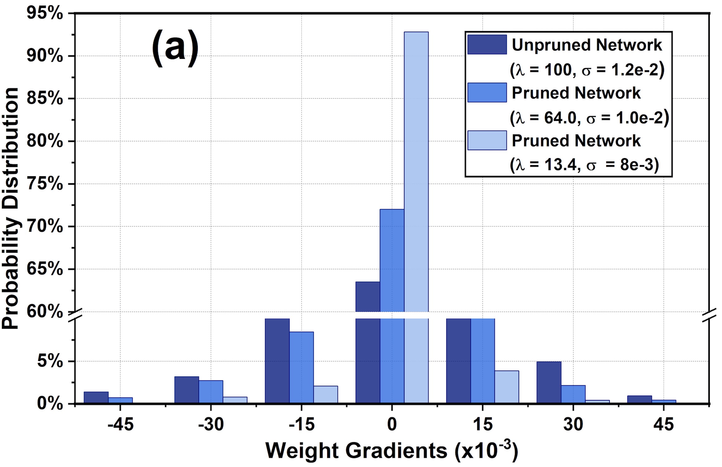
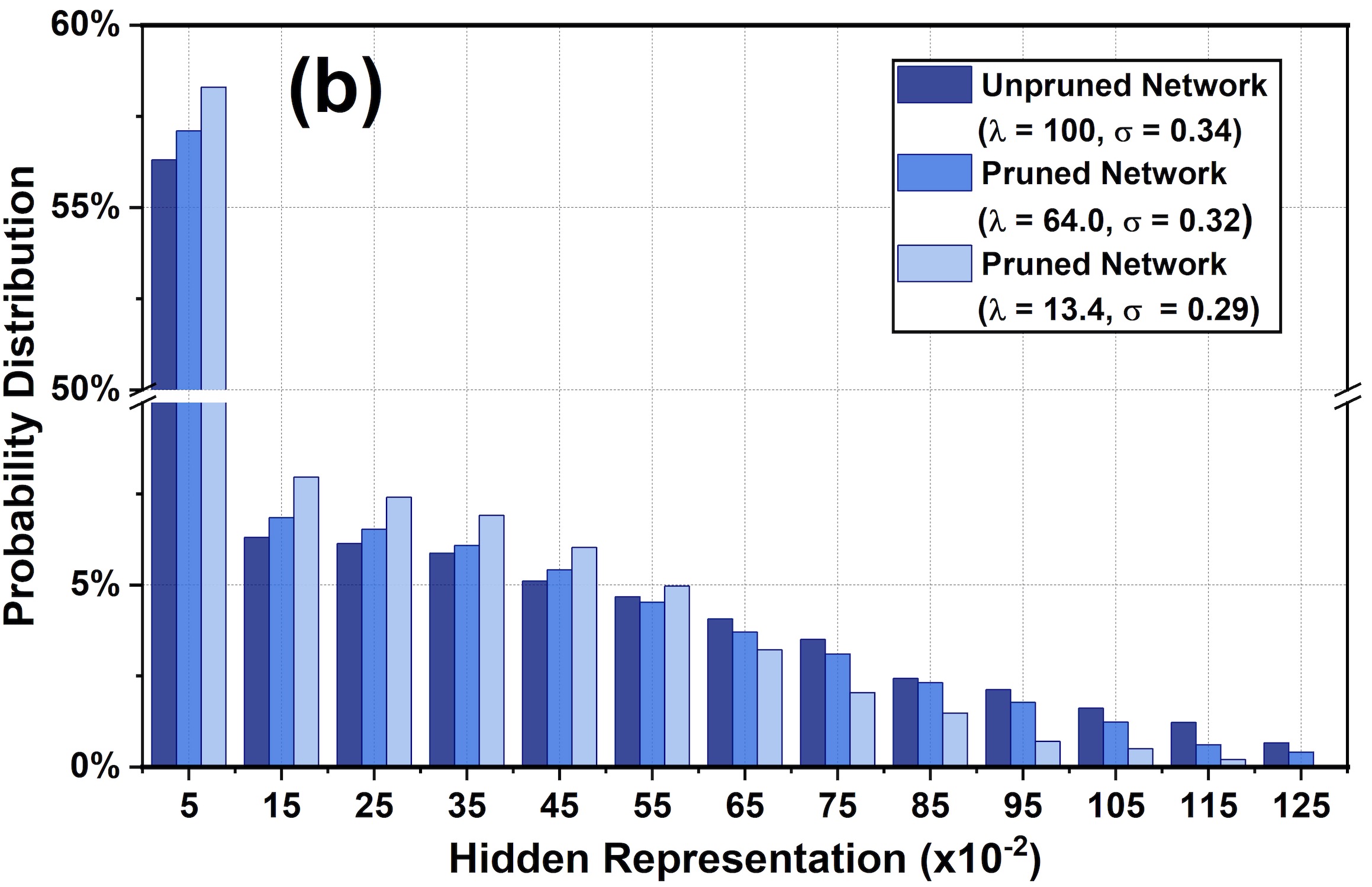
Figure 3: (a) The distribution of weight gradients when iteratively pruning a fully connected ReLU-based network using global magnitude (Han et al. 2015), where $\lambda$ is the percent of weights remaining and $\sigma$ is the standard deviation of the distribution. (b) The corresponding distribution of hidden representations (i.e., post-activation outputs of all hidden layers). The main difference with Fig. 1 is that the batch normalization is used here.

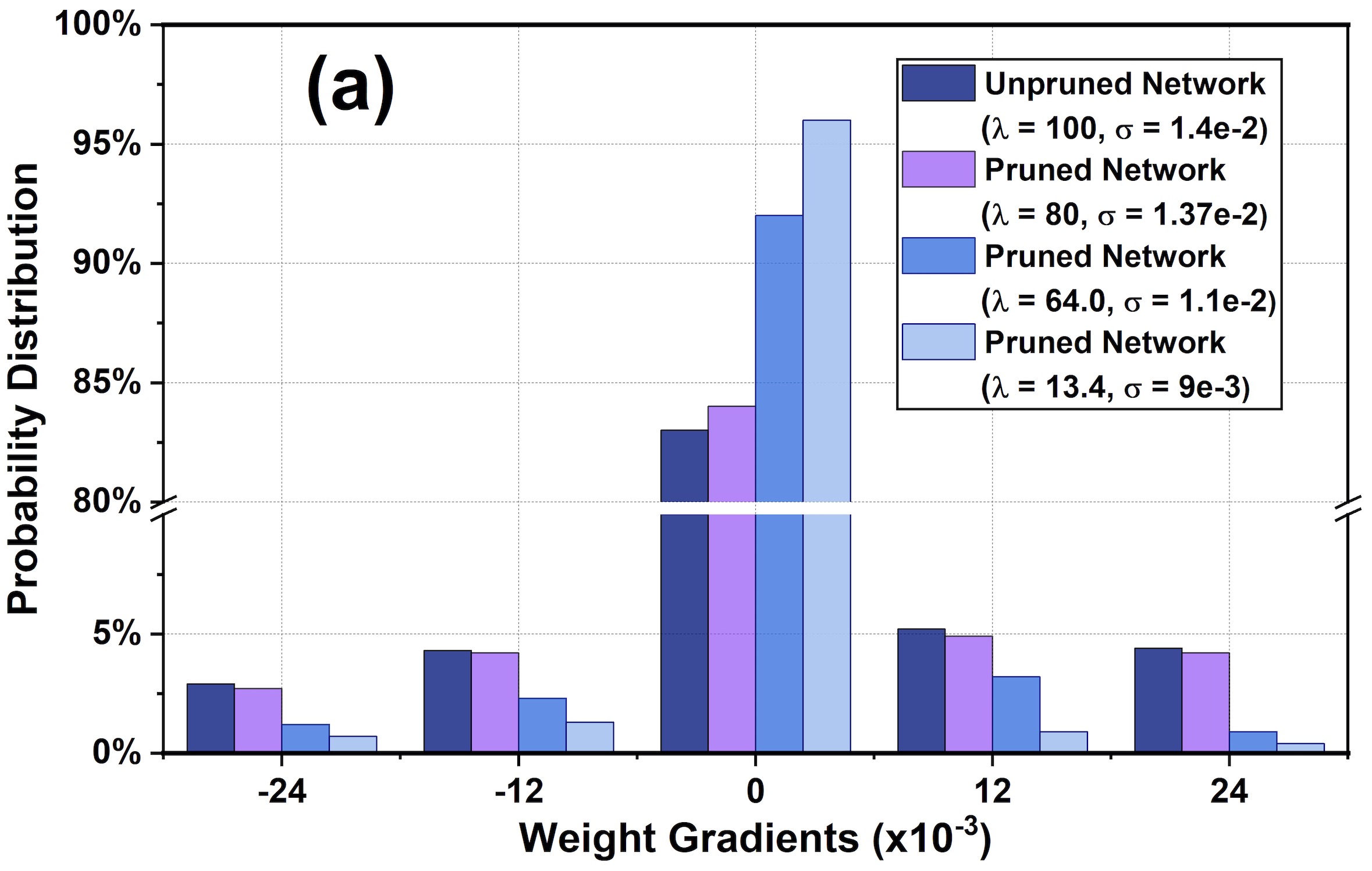
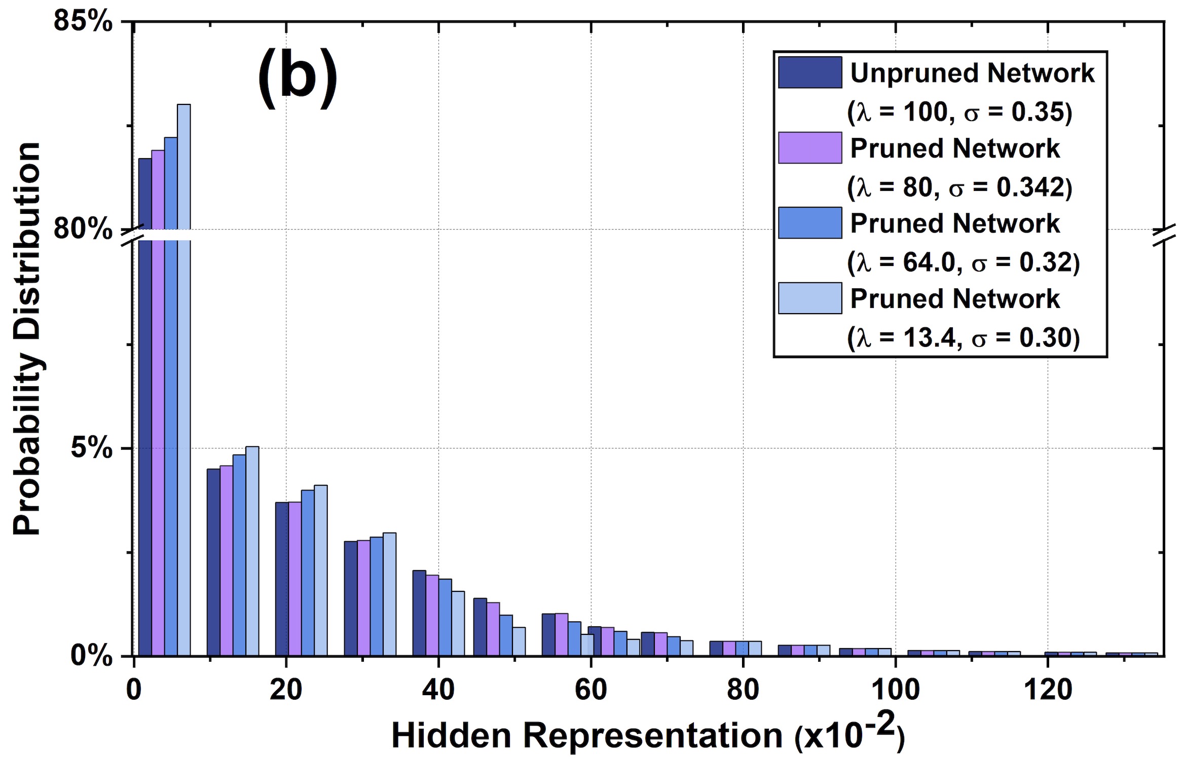
Figure 4: (a) The distribution of weight gradients when iteratively pruning the AlexNet network using the layer magnitude pruning method, where $\lambda$ is the percent of weights remaining and $\sigma$ is the standard deviation of the distribution. (b) The corresponding distribution of hidden representations (i.e., post-activation outputs of all hidden layers). Please note that there is a line breaker in the vertical axis.

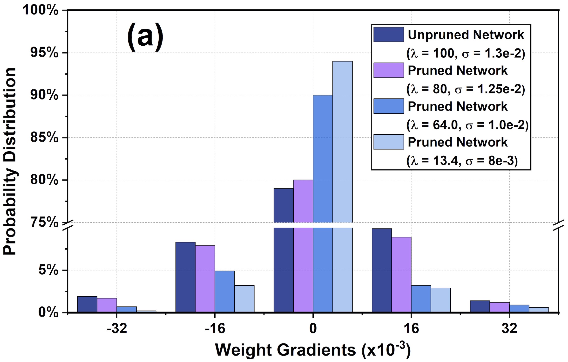
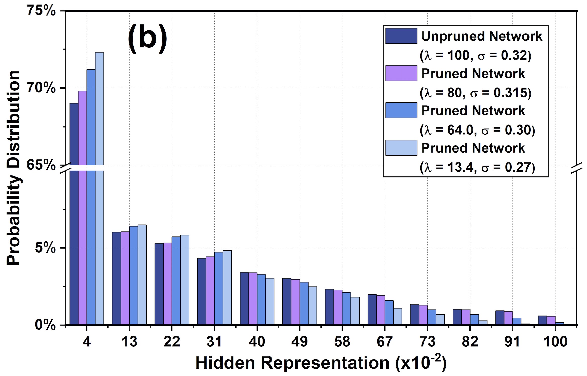
Figure 5: (a) The distribution of weight gradients when iteratively pruning the ResNet-20 network using the global gradient pruning method, where $\lambda$ is the percent of weights remaining and $\sigma$ is the standard deviation of the distribution. (b) The corresponding distribution of hidden representations (i.e., post-activation outputs of all hidden layers). Please note that there is a line breaker in the vertical axis.

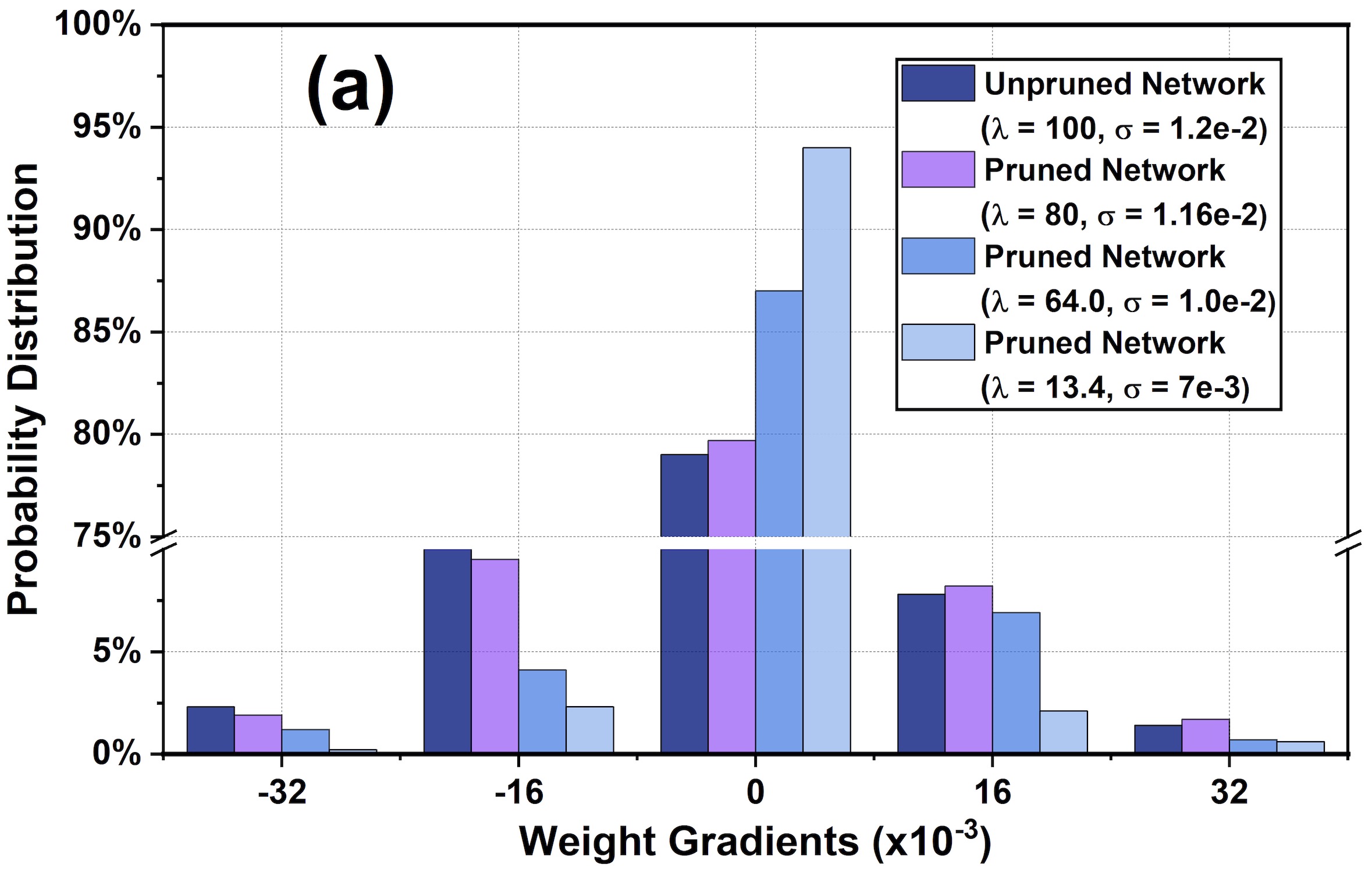
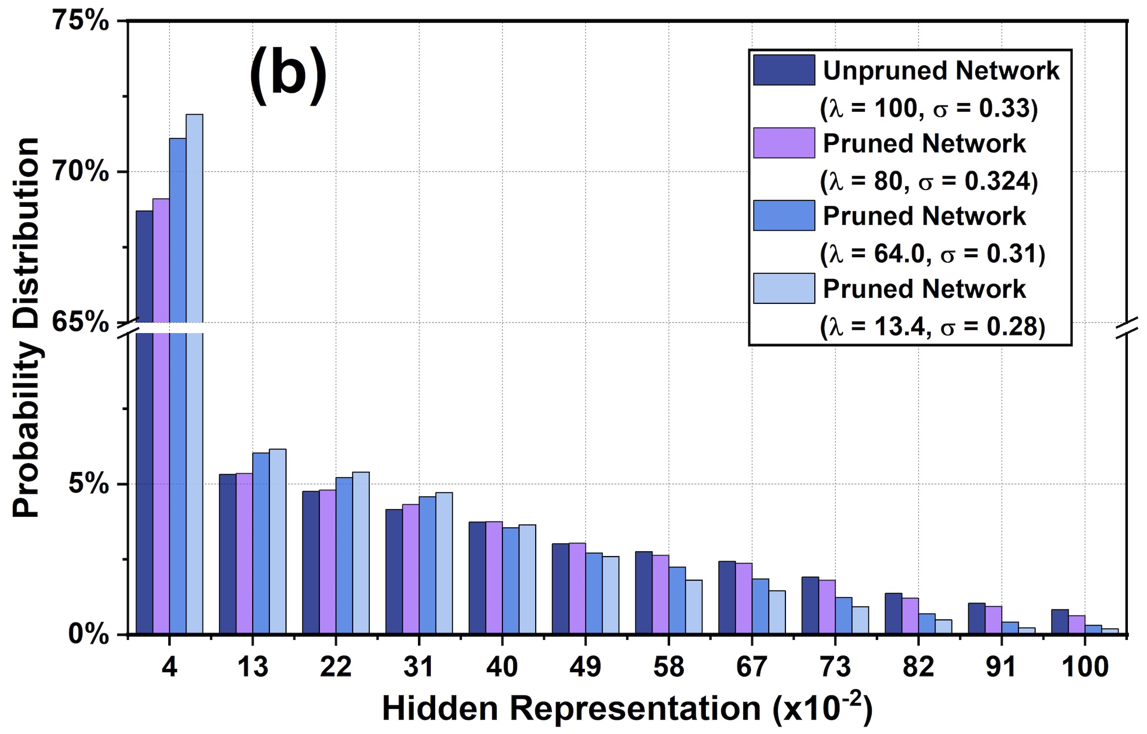
Figure 6: (a) The distribution of weight gradients when iteratively pruning the VGG-19 network using the structured filter pruning method (Li et al. 2017), where $\lambda$ is the percent of weights remaining and $\sigma$ is the standard deviation of the distribution. (b) The corresponding distribution of hidden representations (i.e., post-activation outputs of all hidden layers). Please note that there is a line breaker in the vertical axis.

B.2 Performance Comparison using Adam and RMSProp

In this subsection, we show the performance comparison between the proposed SILO and selected LR benchmarks using Adam (Kingma and Ba 2014) and RMSProp (Tieleman and Hinton 2012) optimizers. The experimental results summarized in Tables 9 - 10 largely mirror those in Table 3. Specifically, the proposed SILO outperforms the best performing benchmark by a range of 0.8% -2.7% in pruned networks.

Params: 227K; Train Steps: 63K Iters; Batch: 128; Pruning Rate: 0.2
(1) constant LR (8e-4) (2) LR decay (3e-3, 63K)
(3) cyclical LR (0, 3e-2, 8K) (4) LR-warmup (3e-3, 20K, 20K, 25K, Nil)
(5) SILO (3e-3,4e-3,20K,20K,25K,Nil)

$\lambda$	100	32.9	21.1	5.72	2.03
(1) constant LR	88.4$\pm$0.4	84.8$\pm$0.6	83.5$\pm$0.6	75.5$\pm$1.2	67.1$\pm$1.7
(2) LR decay	88.6$\pm$0.3	87.1$\pm$0.7	83.7$\pm$0.9	76.1$\pm$0.8	66.0$\pm$1.3
(3) cyclical LR	88.9$\pm$0.3	86.9$\pm$0.5	84.1$\pm$0.3	77.0$\pm$0.9	64.4$\pm$1.1
(4) LR-warmup	89.1$\pm$0.3	87.2$\pm$0.4	84.5$\pm$0.6	75.2$\pm$1.1	65.1$\pm$1.9
(5) SILO	89.2$\pm$0.2	87.9$\pm$0.3	86.3$\pm$0.5	79.5$\pm$1.7	71.7$\pm$2.3

Table 9: Performance comparison (averaged top-1 test accuracy $\pm$ std over 5 runs) of iteratively pruning ResNet-20 on CIFAR-10 dataset using the global magnitude pruning method (Han et al. 2015) and the Adam optimizer (Kingma and Ba 2014).

Params: 227K; Train Steps: 63K Iters; Batch: 128; Pruning Rate: 0.2
(1) constant LR (6e-4) (2) LR decay (2e-3, 63K)
(3) cyclical LR (0, 3e-2, 10K) (4) LR-warmup (1e-3, 20K, 20K, 25K, Nil)
(5) SILO (1e-3,2e-3,20K,20K,25K,Nil)

$\lambda$	100	32.9	21.1	5.72	2.03
(1) constant LR	87.9$\pm$0.3	83.4$\pm$0.4	81.5$\pm$0.9	65.5$\pm$1.9	55.1$\pm$2.3
(2) LR decay	88.4$\pm$0.2	84.8$\pm$0.6	77.8$\pm$0.9	67.1$\pm$1.4	58.3$\pm$1.6
(3) cyclical LR	88.1$\pm$0.3	84.7$\pm$0.5	81.9$\pm$0.7	67.5$\pm$0.9	56.3$\pm$1.7
(4) LR-warmup	88.9$\pm$0.2	85.1$\pm$0.5	81.7$\pm$0.4	67.3$\pm$1.3	57.1$\pm$1.4
(5) SILO	88.7$\pm$0.3	86.1$\pm$0.4	83.1$\pm$0.6	72.5$\pm$1.3	63.5$\pm$1.9

Table 10: Performance comparison (averaged top-1 test accuracy $\pm$ std over 5 runs) of iteratively pruning ResNet-20 on CIFAR-10 dataset using the global magnitude pruning method (Han et al. 2015) and the RMSProp optimizer (Tieleman and Hinton 2012).

B.3 More Experimental Results on Comparing SILO to an Oracle

We show the performance between SILO’s max_lr to that of an Oracle using ResNet-20 with global gradient on the CIFAR-10 dataset in Table 11. It can be seen that the max_lr estimated by SILO falls in the Oracle optimized max_lr interval at each pruning cycle, meaning that the performance of SILO is competitive to the Oracle. Via this experiment on ResNet-20, we highlight the competitiveness of the proposed SILO again.

Percent of Weights Remaining, $\lambda$	100	51.3	41.1	32.9	21.1
Oracle max_lr	3.4	3.8	4.6	5.6	6.2
Oracle interval	[2.8, 3.6]	[3.4, 4.2]	[3.8, 5.2]	[5.4, 6.6]	[5.4, 6.8]
SILO max_lr	3	3.2	4.7	6.4	6.9

Table 11: Comparison between Oracle tuned max_lr, Oracle optimized max_lr interval (both obtained via grid search) and max_lr estimated by SILO when iteratively pruning ResNet-20 on the CIFAR-10 dataset using the global magnitude (Han et al. 2015).

B.4 Experimental Results for More Values of $\lambda$

We note that, in Tables 1 - 6, we only show the experimental results for some key values of $\lambda$. In this subsection, we show the results for more values of $\lambda$ in Tables 13 - 18. The LR schedules (i.e., LR-warmup) from Table 13 - 17 are from (Frankle and Carbin 2019), (Frankle et al. 2020), (Zhao et al. 2019), (Chin et al. 2020) and (Renda, Frankle, and Carbin 2019), respectively. The LR schedule (i.e., cosine decay) in Table 18 is from (Dosovitskiy et al. 2020). The implementation details are provided in the top row of each table and the descriptions of each benchmark LR schedule are summarized in Table 12. It should be noted that, for the IMP method examined in this work, we rewind the unpruned weights to their values during training (e.g., epoch 6), in order to obtain a more stable subnetwork (Frankle et al. 2019).

Due to the width of these tables, we rotate them and present the results in the landscape style. We observe that the performance of SILO for other values of $\lambda$ still outperforms the selected LR schedule benchmarks. For example, in Table 15, we find that SILO achieves an improvement of 4.0% at $\lambda$ = 5.72 compared to LR warmup.

Schedule	Description (Iters: Iterations)
LR decay (a, b)	linearly decay the value of LR from a over b Iters.
cyclical LR (a, b, c)	linearly vary between a and b with a step size of c Iters.
LR warmup (a, b, c, d, e)	increase to a over b Iters, 10x drop at c, d, e Iters.
SILO ($\epsilon$, $\delta$, b, c, d, e)	LR warmup (max_lr, b, c, d, e), where max_lr increases
	from $\epsilon$ to $\epsilon+\delta$ during iterative pruning (see (3)).

Table 12: Descriptions of LR schedule benchmarks and the proposed SILO.

Params: 227K	Train Steps: 63K Iters	Batch: 128	Batch Norm: Yes	Optimizer: SGD	Rate: 0.2

Percent of Weights Remaining, $\lambda$	100	64	40.9	32.8	26.2	13.4	8.59	5.72
constant LR (1e-2)	90.4$\pm$0.4	89.7$\pm$0.5	88.9$\pm$0.7	88.1$\pm$0.9	87.5$\pm$0.8	86.0$\pm$0.9	82.8$\pm$0.9	79.1$\pm$0.8
LR decay (3e-2, 63K)	91.2$\pm$0.4	91.0$\pm$0.3	90.3$\pm$0.5	89.8$\pm$0.4	89.0$\pm$0.7	87.7$\pm$0.6	83.9$\pm$0.6	79.8$\pm$0.7
cyclical LR (0, 3e-2, 8K)	90.8$\pm$0.3	90.4$\pm$0.5	90.1$\pm$0.4	89.7$\pm$0.6	88.2$\pm$0.7	87.6$\pm$0.8	84.1$\pm$0.6	80.3$\pm$0.7
LR-warmup (3e-2, 20K, 20K, 25K, Nil)	91.7$\pm$0.2	91.5$\pm$0.3	90.8$\pm$0.5	90.3$\pm$0.4	89.8$\pm$0.6	88.2$\pm$0.6	85.9$\pm$0.9	81.2$\pm$1.1
SILO (3e-2, 4e-2, 20K, 20K, 25K, Nil)	91.7$\pm$0.2	91.9$\pm$0.4	91.2$\pm$0.6	90.8$\pm$0.5	90.3$\pm$0.4	89.7$\pm$0.5	87.5$\pm$0.8	82.7$\pm$1.2

Table 13: Performance comparison (averaged top-1 test accuracy $\pm$ std over 5 runs) of pruning ResNet-20 on CIFAR-10 dataset using the global magnitude pruning method (Blalock et al. 2020). LR-warmup is the standard implementation used in (Frankle and Carbin 2019; Frankle et al. 2020).

Params: 139M	Train Steps: 63K Iters	Batch: 128	Batch Norm: Yes	Optimizer: SGD	Rate: 0.2

Percent of Weights Remaining, $\lambda$	100	64	40.9	32.8	26.2	13.4	8.59	5.72
constant LR (8e-3)	91.3$\pm$0.3	90.5$\pm$0.5	89.5$\pm$0.6	88.8$\pm$0.6	87.4$\pm$0.7	85.8$\pm$0.6	82.2$\pm$1.4	73.7$\pm$1.3
LR decay (1e-2, 63K)	92.0$\pm$0.5	90.9$\pm$0.5	90.2$\pm$0.5	89.4$\pm$0.4	88.6$\pm$0.5	87.4$\pm$0.6	83.3$\pm$0.8	75.4$\pm$0.9
cyclical LR (0, 3e-2, 15K)	92.3$\pm$0.6	91.2$\pm$0.6	90.4$\pm$0.4	89.8$\pm$0.5	89.1$\pm$0.6	88.6$\pm$0.8	83.7$\pm$1.0	75.7$\pm$1.2
LR-warmup (1e-1, 10K, 32K, 48K, Nil)	92.2$\pm$0.3	91.3$\pm$0.2	90.6$\pm$0.4	90.2$\pm$0.5	89.8$\pm$0.8	89.2$\pm$0.8	84.5$\pm$0.9	76.5$\pm$1.1
SILO (4e-2, 6e-2, 10K, 32K, 48K, Nil)	92.6$\pm$0.4	91.8$\pm$0.6	90.9$\pm$0.5	90.6$\pm$0.6	90.3$\pm$0.6	89.8$\pm$0.9	86.1$\pm$0.8	78.5$\pm$1.0

Table 14: Performance comparison (averaged top-1 test accuracy $\pm$ std over 5 runs) of pruning VGG-19 on CIFAR-10 dataset using the global gradient pruning method (Blalock et al. 2020). LR-warmup is the standard implementation used in (Frankle and Carbin 2019; Frankle et al. 2020; Liu et al. 2019).

Params: 1M	Train Steps: 117K Iters	Batch: 128	Batch Norm: Yes	Optimizer: SGD	Pruning Rate: 0.2

Percent of Weights Remaining, $\lambda$	100	64	40.9	32.8	26.2	13.4	8.59	5.72
constant LR (1e-2)	73.7$\pm$0.4	72.8$\pm$0.4	71.4$\pm$0.5	70.3$\pm$0.8	68.1$\pm$0.7	63.5$\pm$0.6	60.8$\pm$1.1	59.1$\pm$1.2
LR decay (4e-2, 117K)	74.3$\pm$0.3	73.5$\pm$0.9	72.2$\pm$0.4	71.2$\pm$0.8	69.0$\pm$0.6	64.7$\pm$0.7	62.6$\pm$1.2	60.3$\pm$1.4
cyclical LR (0, 4e-2, 24K)	74.4$\pm$0.4	73.2$\pm$0.5	72.0$\pm$0.3	70.9$\pm$0.6	69.4$\pm$0.6	65.1$\pm$0.9	63.0$\pm$1.1	60.8$\pm$1.3
LR-warmup (12e-2, 58K, 58K, 92K, Nil)	74.6$\pm$0.5	73.4$\pm$0.6	72.3$\pm$0.4	71.5$\pm$0.7	69.6$\pm$0.8	65.8$\pm$0.9	63.9$\pm$1.0	61.2$\pm$0.9
SILO (7e-2, 5e-2, 58K, 58K, 92K, Nil)	75.0$\pm$0.5	74.1$\pm$0.3	72.9$\pm$0.6	72.4$\pm$0.7	70.8$\pm$0.8	67.6$\pm$1.2	65.7$\pm$1.1	63.7$\pm$1.0

Table 15: Performance comparison (averaged top-1 test accuracy $\pm$ standard deviation over 5 runs) of pruning DenseNet-40 on CIFAR-100 dataset using LAMP. LR-warmup is adapted from the standard implementation used in (Zhao et al. 2019; Huang et al. 2017).

Params: 2.36M	Train Steps: 78K Iters	Batch: 128	Batch Norm: Yes	Optimizer: SGD	Pruning Rate: 0.2

Percent of Weights Remaining, $\lambda$	100	64	40.9	32.8	26.2	13.4	8.59	5.72
constant LR (1e-2)	72.7$\pm$0.2	71.5$\pm$0.4	70.4$\pm$0.5	69.8$\pm$1.1	68.2$\pm$0.9	64.5$\pm$0.6	63.8$\pm$1.1	62.1$\pm$1.2
LR decay (15e-1, 78K)	73.3$\pm$0.3	72.1$\pm$0.3	71.8$\pm$0.4	70.9$\pm$1.0	69.4$\pm$0.6	65.9$\pm$0.7	65.1$\pm$0.8	64.0$\pm$1.1
cyclical LR (0, 5e-2, 14K)	73.5$\pm$0.4	72.3$\pm$0.5	72.0$\pm$0.3	71.5$\pm$0.7	69.6$\pm$0.6	66.7$\pm$0.9	65.3$\pm$1.0	64.3$\pm$1.2
LR-warmup (1e-1, 23K, 23K, 46K, 62K)	73.7$\pm$0.4	72.5$\pm$0.4	72.3$\pm$0.5	72.1$\pm$0.8	70.5$\pm$0.9	67.3$\pm$0.8	66.2$\pm$1.1	64.8$\pm$1.5
SILO (5e-2, 5e-2, 23K, 23K, 46K, 92K)	74.0$\pm$0.5	73.0$\pm$0.3	72.9$\pm$0.8	72.5$\pm$0.6	71.0$\pm$0.7	68.8$\pm$0.8	67.6$\pm$1.2	66.8$\pm$1.4

Table 16: Performance comparison (averaged top-1 test accuracy $\pm$ standard deviation over 5 runs) of pruning MobileNetV2 on CIFAR-100 dataset using LAP. LR-warmup is adapted from the standard implementation used in (Chin et al. 2020).

Params: 25.5M	Train Steps: 70K Iters	Batch: 128	Batch Norm: Yes	Optimizer: SGD	Rate: 0.2

Percent of Weights Remaining, $\lambda$	100	64	40.9	32.8	26.2	13.4	8.59	5.72
constant LR (1e-2)	75.3$\pm$0.2	75.2$\pm$0.3	74.6$\pm$0.7	74.2$\pm$0.8	73.9$\pm$0.7	72.2$\pm$0.9	70.5$\pm$0.6	69.2$\pm$0.9
LR decay (3e-2, 70K	76.5$\pm$0.2	76.1$\pm$0.5	75.8$\pm$0.6	75.6$\pm$0.5	75.1$\pm$0.5	73.9$\pm$0.7	72.7$\pm$0.8	70.5$\pm$0.6
cyclical LR (0, 5e-2, 20K)	76.8$\pm$0.3	76.9$\pm$0.5	77.0$\pm$0.6	76.5$\pm$0.5	75.5$\pm$0.6	74.5$\pm$0.6	73.4$\pm$0.8	71.2$\pm$0.7
LR-warmup (1e-1, 4K, 23K, 46K, 62K)	77.0$\pm$0.1	77.2$\pm$0.2	76.9$\pm$0.5	76.6$\pm$0.2	75.8 $\pm$0.3	75.2$\pm$0.4	73.8$\pm$0.5	71.5$\pm$0.4
SILO (5e-2, 5e-2, 4K, 23K, 46K, 62K)	77.2$\pm$0.2	77.4$\pm$0.3	77.0$\pm$0.4	76.8$\pm$0.4	76.1$\pm$0.7	75.8$\pm$0.6	75.2$\pm$0.8	73.8$\pm$0.6

Table 17: Performance comparison (averaged top-1 test accuracy $\pm$ standard deviation over 5 runs) of pruning ResNet-50 on ImageNet dataset using the IMP pruning method (Le and Yang 2015). LR-warmup is adapted from the standard implementation used in (Frankle et al. 2020; Renda, Frankle, and Carbin 2019).

Params: 86M	Train Steps: 2K Iters	Batch: 1024	Batch Norm: Yes	Optimizer: Adam	Rate: 0.2

Percent of Weights Remaining, $\lambda$	100	64	40.9	32.8	26.2	13.4	8.59	5.72
constant LR (5e-5)	97.4$\pm$0.2	97.6 $\pm$0.3	97.5 $\pm$0.4	96.4 $\pm$0.5	96.0$\pm$0.7	86.3$\pm$0.6	83.0$\pm$0.9	80.1$\pm$0.8
cosine decay (1e-4, 2K	98.0$\pm$0.3	98.2 $\pm$ 0.3	97.9 $\pm$ 0.4	97.2 $\pm$ 0.2	96.5$\pm$0.6	87.7$\pm$0.5	84.1$\pm$1.0	81.6$\pm$1.1
cyclical LR (0, 1e-4, 2K)	97.8$\pm$0.4	98.0 $\pm$ 0.2	97.8 $\pm$ 0.3	97.0 $\pm$ 0.2	96.5$\pm$0.6	87.2$\pm$0.9	83.4$\pm$0.6	81.0$\pm$1.1
LR-warmup (4e-4, 0.3K, 0.5K, 0.9K, 1.3K)	98.0$\pm$0.3	98.4 $\pm$0.3	97.8 $\pm$0.5	97.3 $\pm$0.6	96.8$\pm$0.7	88.1$\pm$0.9	84.4$\pm$0.8	82.1$\pm$0.9
SILO (1e-4, 3e-4, 0.3K, 0.5K, 0.9K, 1.3K)	98.0$\pm$0.3	98.5$\pm$0.4	98.0$\pm$0.3	97.7$\pm$0.5	97.4$\pm$0.6	89.2$\pm$0.8	85.5$\pm$0.9	83.4$\pm$0.8

Table 18: Performance comparison (averaged top-1 test accuracy $\pm$ standard deviation over 5 runs) of pruning pruning Vision Transformer (ViT-B-16) on CIFAR-10 using IMP (Frankle and Carbin 2019). Cosine decay is the standard implementation used in (Dosovitskiy et al. 2020).

References

- Allen-Zhu, Li, and Song (2019) Allen-Zhu, Z.; Li, Y.; and Song, Z. 2019. A Convergence Theory for Deep Learning via Over-Parameterization. In Proceedings of the International Conference on Machine Learning (ICML), volume 97, 242–252.
- An et al. (2017) An, W.; et al. 2017. Exponential decay sine wave learning rate for fast deep neural network training. In 2017 IEEE Visual Communications and Image Processing (VCIP), 1–4. IEEE.
- Andrews (1998) Andrews, L. C. 1998. Special functions of mathematics for engineers, volume 49. Spie Press.
- Arora, Cohen, and Hazan (2018) Arora, S.; Cohen, N.; and Hazan, E. 2018. On the optimization of deep networks: Implicit Acceleration by overparameterization. In Proceedings of the International Conference on Machine Learning (ICML), volume 80, 244–253.
- Bengio (2012) Bengio, Y. 2012. Practical recommendations for gradient-based training of deep architectures. In Neural networks: Tricks of the trade, 437–478. Springer.
- Blalock et al. (2020) Blalock, D.; et al. 2020. What is the State of Neural Network Pruning? In Proceedings of the Machine Learning and Systems (MLSys).
- Chin et al. (2020) Chin, T.-W.; Ding, R.; Zhang, C.; and Marculescu, D. 2020. Towards efficient model compression via learned global ranking. In Proceedings of the IEEE/CVF Conference on Computer Vision and Pattern Recognition (CVPR), 1518–1528.
- Deng et al. (2009) Deng, J.; et al. 2009. Imagenet: A large-scale hierarchical image database. In 2009 IEEE conference on computer vision and pattern recognition, 248–255. IEEE.
- Denil et al. (2013) Denil, M.; et al. 2013. Predicting parameters in deep learning. In Proceedings of the Advances in Neural Information Processing Systems (Neurips), 2148–2156.
- Dosovitskiy et al. (2020) Dosovitskiy, A.; Beyer, L.; Kolesnikov, A.; Weissenborn, D.; Zhai, X.; Unterthiner, T.; Dehghani, M.; Minderer, M.; Heigold, G.; Gelly, S.; et al. 2020. An image is worth 16x16 words: Transformers for image recognition at scale. arXiv preprint arXiv:2010.11929.
- Frankle and Carbin (2019) Frankle, J.; and Carbin, M. 2019. The Lottery Ticket Hypothesis: Finding Sparse, Trainable Neural Networks. In Proceedings of the International Conference on Learning Representations (ICLR).
- Frankle et al. (2019) Frankle, J.; Dziugaite, G. K.; Roy, D. M.; and Carbin, M. 2019. Stabilizing the lottery ticket hypothesis. arXiv preprint arXiv:1903.01611.
- Frankle et al. (2020) Frankle, J.; et al. 2020. Linear Mode Connectivity and the Lottery Ticket Hypothesis. In Proceedings of the International Conference on Machine Learning (ICML), 3259–3269.
- Gandikota et al. (2021) Gandikota, V.; et al. 2021. vqsgd: Vector quantized stochastic gradient descent. In Proceedings of the International Conference on Artificial Intelligence and Statistics, 2197–2205.
- Ge et al. (2019) Ge, R.; et al. 2019. The step decay schedule: A near optimal, geometrically decaying learning rate procedure for least squares. arXiv preprint arXiv:1904.12838.
- Goodfellow, Bengio, and Courville (2016) Goodfellow, I.; Bengio, Y.; and Courville, A. 2016. Deep learning. MIT press.
- Han, Mao, and Dally (2015) Han, S.; Mao, H.; and Dally, W. J. 2015. Deep compression: Compressing deep neural networks with pruning, trained quantization and huffman coding. arXiv preprint arXiv:1510.00149.
- Han et al. (2015) Han, S.; et al. 2015. Learning both weights and connections for efficient neural network. In Proceedings of the Advances in Neural Information Processing Systems (Neurips), 1135–1143.
- Hassibi and Stork (1993) Hassibi, B.; and Stork, D. G. 1993. Second order derivatives for network pruning: Optimal brain surgeon. In Proceedings of the Advances in Neural Information Processing Systems (Neurips), 164–171.
- He et al. (2016) He, K.; et al. 2016. Deep residual learning for image recognition. In Proceedings of the IEEE Conference on Computer Vision and Pattern Recognition, 770–778.
- He et al. (2019) He, T.; et al. 2019. Bag of tricks for image classification with convolutional neural networks. In Proceedings of the IEEE/CVF Conference on Computer Vision and Pattern Recognition (CVPR), 558–567.
- He et al. (2020) He, Y.; et al. 2020. Learning Filter Pruning Criteria for Deep Convolutional Neural Networks Acceleration. In Proceedings of the IEEE/CVF Conference on Computer Vision and Pattern Recognition (CVPR).
- Hu et al. (2016) Hu, H.; et al. 2016. Network trimming: A data-driven neuron pruning approach towards efficient deep architectures. arXiv preprint arXiv:1607.03250.
- Huang et al. (2017) Huang, G.; et al. 2017. Densely connected convolutional networks. In Proceedings of the IEEE/CVF Conference on Computer Vision and Pattern Recognition, 4700–4708.
- Ioffe and Szegedy (2015) Ioffe, S.; and Szegedy, C. 2015. Batch normalization: Accelerating deep network training by reducing internal covariate shift. In Proceedings of the International Conference on Machine Learning (ICML), volume 37, 448–456.
- Jentzen et al. (2021) Jentzen, A.; et al. 2021. Strong error analysis for stochastic gradient descent optimization algorithms. IMA Journal of Numerical Analysis, 41(1): 455–492.
- Kingma and Ba (2014) Kingma, D. P.; and Ba, J. 2014. Adam: A Method for Stochastic Optimization. arXiv:1412.6980.
- Krizhevsky and Hinton (2010) Krizhevsky, A.; and Hinton, G. 2010. Convolutional deep belief networks on cifar-10. Unpublished manuscript, 40(7): 1–9.
- Krizhevsky et al. (2009) Krizhevsky, A.; et al. 2009. Learning multiple layers of features from tiny images.
- Le and Yang (2015) Le, Y.; and Yang, X. 2015. Tiny imagenet visual recognition challenge. CS 231N.
- LeCun, Denker, and Solla (1990) LeCun, Y.; Denker, J. S.; and Solla, S. A. 1990. Optimal brain damage. In Proceedings of the Advances in Neural Information Processing Systems (Neurips), 598–605.
- Lee et al. (2020) Lee, J.; Park, S.; Mo, S.; Ahn, S.; and Shin, J. 2020. Layer-adaptive Sparsity for the Magnitude-based Pruning. In International Conference on Learning Representations (ICLR).
- Lee et al. (2019) Lee, N.; et al. 2019. SNIP: Single-shot network pruning based on connection sensitivity. In Proceedings of the International Conference on Learning Representations (ICLR).
- Li et al. (2017) Li, H.; et al. 2017. Pruning filters for efficient convnets. In Proceedings of the International Conference on Learning Representations (ICLR).
- Lin et al. (2020) Lin, M.; Ji, R.; Wang, Y.; Zhang, Y.; Zhang, B.; Tian, Y.; and Shao, L. 2020. Hrank: Filter pruning using high-rank feature map. In Proceedings of the IEEE/CVF Conference on Computer Vision and Pattern Recognition (CVPR), 1529–1538.
- Liu, Simonyan, and Yang (2019) Liu, H.; Simonyan, K.; and Yang, Y. 2019. DARTS: Differentiable architecture search. In Proceedings of the International Conference on Learning Representations (ICLR).
- Liu and et al (2021) Liu, S.; and et al. 2021. Sparse Training via Boosting Pruning Plasticity with Neuroregeneration. In Advances in Neural Information Processing Systems, volume 34, 9908–9922.
- Liu et al. (2021) Liu, Z.; Lin, Y.; Cao, Y.; Hu, H.; Wei, Y.; Zhang, Z.; Lin, S.; and Guo, B. 2021. Swin transformer: Hierarchical vision transformer using shifted windows. In Proceedings of the IEEE/CVF International Conference on Computer Vision, 10012–10022.
- Liu et al. (2019) Liu, Z.; et al. 2019. Rethinking the value of network pruning. In Proceedings of the International Conference on Learning Representations (ICLR).
- Luo and Wu (2020) Luo, J.-H.; and Wu, J. 2020. Neural Network Pruning with Residual-Connections and Limited-Data. In Proceedings of the IEEE/CVF Conference on Computer Vision and Pattern Recognition (CVPR), 1458–1467.
- Luo, Wu, and Lin (2017) Luo, J.-H.; Wu, J.; and Lin, W. 2017. Thinet: A filter level pruning method for deep neural network compression. In Proceedings of the IEEE International Conference on Computer Vision (ICCV), 5058–5066.
- Malach et al. (2020) Malach, E.; et al. 2020. Proving the lottery ticket hypothesis: Pruning is all you need. In Proceedings of the International Conference on Machine Learning (ICML), 6682–6691.
- Mehta (2019) Mehta, R. 2019. Sparse Transfer Learning via Winning Lottery Tickets. In Proceedings of the Advances in Neural Information Processing Systems Workshop on Learning Transferable Skills.
- Molchanov et al. (2017) Molchanov, P.; et al. 2017. Pruning convolutional neural networks for resource efficient inference. Proceedings of the International Conference on Learning Representations (ICLR).
- Molchanov et al. (2019) Molchanov, P.; et al. 2019. Importance estimation for neural network pruning. In Proceedings of the IEEE/CVF Conference on Computer Vision and Pattern Recognition (CVPR), 11264–11272.
- Park et al. (2020) Park, S.; Lee, J.; Mo, S.; and Shin, J. 2020. Lookahead: A far-sighted alternative of magnitude-based pruning.
- Renda, Frankle, and Carbin (2019) Renda, A.; Frankle, J.; and Carbin, M. 2019. Comparing rewinding and fine-tuning in neural network pruning. In International Conference on Learning Representations (ICLR).
- Ruder (2016) Ruder, S. 2016. An overview of gradient descent optimization algorithms. arXiv preprint arXiv:1609.04747.
- Sandler et al. (2018) Sandler, M.; Howard, A.; Zhu, M.; Zhmoginov, A.; and Chen, L.-C. 2018. Mobilenetv2: Inverted residuals and linear bottlenecks. In Proceedings of the IEEE conference on computer vision and pattern recognition, 4510–4520.
- Scott (2009) Scott, D. W. 2009. Sturges’ rule. Wiley Interdisciplinary Reviews: Computational Statistics, 1(3): 303–306.
- Simonyan and Zisserman (2014) Simonyan, K.; and Zisserman, A. 2014. Very deep convolutional networks for large-scale image recognition. arXiv preprint arXiv:1409.1556.
- Smith (2017) Smith, L. N. 2017. Cyclical learning rates for training neural networks. In 2017 IEEE Winter Conference on Applications of Computer Vision (WACV), 464–472. IEEE.
- Tan and Motani (2020) Tan, C. M. J.; and Motani, M. 2020. DropNet: Reducing Neural Network Complexity via Iterative Pruning. In Proceedings of the International Conference on Machine Learning (ICML), 9356–9366. PMLR.
- Theis et al. (2018) Theis, L.; et al. 2018. Faster gaze prediction with dense networks and fisher pruning. arXiv preprint arXiv:1801.05787.
- Tieleman and Hinton (2012) Tieleman, T.; and Hinton, G. 2012. Lecture 6.5-rmsprop: Divide the gradient by a running average of its recent magnitude. COURSERA: Neural networks for machine learning, 4(2): 26–31.
- Wang et al. (2020a) Wang, T.; et al. 2020a. APQ: Joint Search for Network Architecture, Pruning and Quantization Policy. In Proceedings of the IEEE/CVF Conference on Computer Vision and Pattern Recognition (CVPR).
- Wang et al. (2020b) Wang, Y.; et al. 2020b. Dynamic Network Pruning with Interpretable Layerwise Channel Selection. In Proceedings of the AAAI Conference on Artificial Intelligence, volume 34, 6299–6306.
- Wang et al. (2020c) Wang, Y.; et al. 2020c. Pruning from scratch. In Proceedings of the AAAI Conference on Artificial Intelligence, volume 34, 12273–12280.
- Wang, Li, and Wang (2021) Wang, Z.; Li, C.; and Wang, X. 2021. Convolutional Neural Network Pruning With Structural Redundancy Reduction. In Proceedings of the IEEE/CVF Conference on Computer Vision and Pattern Recognition (CVPR), 14913–14922.
- Xiao, Wang, and Rajasekaran (2019) Xiao, X.; Wang, Z.; and Rajasekaran, S. 2019. AutoPrune: Automatic Network Pruning by Regularizing Auxiliary Parameters. In Proceedings of the Advances in Neural Information Processing Systems (Neurips), 13681–13691.
- Yang et al. (2019) Yang, H.; et al. 2019. Filter Pruning via Geometric Median for Deep Convolutional Neural Networks Acceleration. In Proceedings of the IEEE Conference on Computer Vision and Pattern Recognition (CVPR), 4335–4344.
- Ye et al. (2020) Ye, M.; et al. 2020. Good subnetworks provably exist: Pruning via greedy forward selection. In Proceedings of the International Conference on Machine Learning (ICML), 10820–10830. PMLR.
- You et al. (2019) You, K.; et al. 2019. How does learning rate decay help modern neural networks? arXiv preprint arXiv:1908.01878.
- Yu et al. (2020) Yu, H. n.; et al. 2020. Playing the lottery with rewards and multiple languages: lottery tickets in RL and NLP. In Proceedings of the International Conference on Learning Representations (ICLR).
- Yu et al. (2018) Yu, R.; et al. 2018. Nisp: Pruning networks using neuron importance score propagation. In Proceedings of the IEEE/CVF Conference on Computer Vision and Pattern Recognition (CVPR), 9194–9203.
- Yuan et al. (2021) Yuan, L.; Hou, Q.; Jiang, Z.; Feng, J.; and Yan, S. 2021. Volo: Vision outlooker for visual recognition. arXiv preprint arXiv:2106.13112.
- Zeiler (2012) Zeiler, M. D. 2012. Adadelta: an adaptive learning rate method. arXiv preprint arXiv:1212.5701.
- Zhao et al. (2019) Zhao, C.; et al. 2019. Variational convolutional neural network pruning. In Proceedings of the IEEE/CVF Conference on Computer Vision and Pattern Recognition (CVPR), 2780–2789.
- Zhou et al. (2019) Zhou, H.; et al. 2019. Deconstructing Lottery Tickets: Zeros, Signs, and the Supermask. In Proceedings of the Advances in Neural Information Processing Systems (Neurips).
- Zhu and Gupta (2018) Zhu, M.; and Gupta, S. 2018. To prune, or not to prune: exploring the efficacy of pruning for model compression. In Proceedings of the International Conference on Learning Representations (ICLR).