Prompting Is Programming: A Query Language for
Large Language Models
Abstract.
Large language models have demonstrated outstanding performance on a wide range of tasks such as question answering and code generation. On a high level, given an input, a language model can be used to automatically complete the sequence in a statistically-likely way. Based on this, users prompt these models with language instructions or examples, to implement a variety of downstream tasks. Advanced prompting methods can even imply interaction between the language model, a user, and external tools such as calculators. However, to obtain state-of-the-art performance or adapt language models for specific tasks, complex task- and model-specific programs have to be implemented, which may still require ad-hoc interaction.
Based on this, we present the novel idea of Language Model Programming (LMP). LMP generalizes language model prompting from pure text prompts to an intuitive combination of text prompting and scripting. Additionally, LMP allows constraints to be specified over the language model output. This enables easy adaption to many tasks while abstracting language model internals and providing high-level semantics.
To enable LMP, we implement LMQL (short for Language Model Query Language), which leverages the constraints and control flow from an LMP prompt to generate an efficient inference procedure that minimizes the number of expensive calls to the underlying language model.
We show that LMQL can capture a wide range of state-of-the-art prompting methods in an intuitive way, especially facilitating interactive flows that are challenging to implement with existing high-level APIs. Our evaluation shows that we retain or increase the accuracy on several downstream tasks, while also significantly reducing the required amount of computation or cost in the case of pay-to-use APIs (26-85% cost savings).
1. Introduction
Large Language Models (Large LMs - LLMs) (Vaswani et al., 2017; Devlin et al., 2019; Radford et al., 2019; Brown et al., 2020) have proven successful at various language-based tasks such as machine translation, text summarization, question answering, reasoning, code generation from text and many more. Due to these results, LMs have become popular beyond the machine learning community and are slowly being integrated into many applications.
(Large) Language Models
Internally, language models operate on tokens, which are different from how humans perceive language. Given the tokenized version of some input, called the prompt, a large language model predicts the next token. That is, over a large vocabulary of tokens it assigns each a score or probability. A decoding procedure is then used, which by invoking the LM multiple times, computes a completion of the prompt. Commonly, the goal is to determine (or approximate) the highest probability continuation, however, as producing a particular token might lower the probability, before a subsequent token increases it, decoding sometimes requires expensive search or backtracking strategies. Nonetheless, LM-based text completion has shown to be very powerful and can be leveraged for a wide range of downstream applications.
Key Challenges in Using Language Models
While the newer generation of language models can be prompted with examples or instructions in a conceptually simple manner, making the best use of these models and keeping up as new models are released requires a deep understanding of their internals, as well as the use of vendor-specific libraries and implementations. For example, as LMs operate on tokens, it can be hard to constrain the decoding procedure to a set of legal words or phrases. Further, many prompting techniques can require back-and-forth interaction between the LM and the user (e.g. chatbots like ChatGPT (OpenAI, 2022)) or very task-specific interfaces (e.g. to perform arithmetic calculations with external control logic). To implement these prompts, a lot of manual work and interaction with a model’s decoding procedure is required, which restricts the generality of the resulting implementations. Lastly, as an LM only produces one (sub-word) token at a time, completing a sequence may require many calls. Also, decoding becomes increasingly expensive as the prefix, the prompt, and the so-far generated response grow. Because of these factors, and as language models are typically very large neural networks, practical inference demands high computational costs and significant latency. In the case of pay-to-use APIs, such as OpenAI’s GPT models, this results in high usage costs per query answered.
This work: Language Model Programming via LMQL
In this work, we propose the idea of language model programming, extending on natural language prompting by additionally allowing lightweight scripting and constraining of outputs. This facilitates a front-end/back-end separation for LM prompting, i.e. allows a user to specify complex interactions, control flow, and constraints without requiring knowledge of an LM’s internals such as tokenization, implementation, and architecture. Further, the constructed programs remain agnostic concerning the underlying LM, greatly improving portability. Overall, Language Model Programming (LMP) retains the simple natural-language-driven interface to LMs but additionally enables precise constraining, scripting, and efficient decoding, which, as of now, is not possible with existing high-level APIs.
To enable LMP, we present a novel language and runtime called the Language Model Query Language (LMQL). LMQL is a high-level language with declarative SQL-like elements and an imperative syntax for scripting. The underlying runtime is compatible with existing LMs and can be supported easily, requiring only a simple change in the decoder logic. LMQL can be used to express a wide variety of existing prompting methods (Reynolds and McDonell, 2021; Wei et al., 2023; Cobbe et al., 2021; Yao et al., 2023; Scholak et al., 2021; Shin et al., 2021) using simple, concise, and vendor-agnostic code. Further, purpose-designed evaluation semantics with support for partial evaluation and lookahead, enable us to optimize query execution end-to-end: LMQL leverages user constraints and scripted prompts to prune the search space of an LM by masking, resulting in an up to 80% reduction of inference cost. We showcase two examples of simple LMQL programs in Fig. 1.
Main Contributions
Our core contributions are:
-
•
We introduce the novel paradigm of language model programming, formulating and addressing several challenges that arise with recent LM prompting techniques (Section 2).
-
•
LMQL, an efficient, high-level query language for LMs with support for scripted prompting and output constraining. (Sections 4 and 3).
-
•
A formal model of eager, partial evaluation semantics based on so-called final and follow abstractions. Using these, we can automatically generate model-specific token masks for LM decoding, given just a set of high-level constraints (Section 5).
-
•
A comprehensive evaluation of LMQL that shows how to express a wide range of common and advanced prompting techniques as simple and concise LMQL programs, which also execute more efficiently, as LMQL reduces inference cost and latency by 26-80% while retaining or slightly improving on task accuracy. (Section 6).
2. Overview: Language Model Programming
In this section we first review how modern language models (LMs) are utilized and the challenges that arise from this. Then, based on examples, we show how Language Model Programming (LMP) can overcome or simplify these challenges and outline the rest of the paper. While our goal with LMP is to improve the usage of state-of-the-art large language models (LLMs), e.g. GPT (Radford et al., 2019) variants, the size of the model does not change how LMP is employed, we thus utilize the acronym LM rather than the more common LLM in the remainder of this text.
2.1. Background: (Large) Language Models
Current language models (Vaswani et al., 2017; Radford et al., 2019; Brown et al., 2020) operate on a vocabulary of (sub-word) tokens. Fig. 2 shows this for a simple example, where we see that common words have their own token (even with a space in front), while more rare words are split into multiple tokens. Similar to formal languages we let denote all possible sequences of tokens over . Given an input sequence of words , a tokenizer then first maps the sequence of words to a sequence of tokens , and then a language model predicts a score for every possible next token. We treat the implementation of as a black box (it does not need to be a neural network), yet in practice most such models are variants of the Transformer architecture (Vaswani et al., 2017). Via the softmax function, the resulting scores can then be turned into a probability distribution over the vocabulary :
Decoding
Based on this, the language model is applied multiple times to produce a sequence for . When we want to pick the -th token, gives a probability distribution over this next token. Several ways of picking from this distribution have been discussed in the literature. Below we review a selection of the most popular ones. Each method is iterated until a special end-of-sequence-token eos is predicted or another stopping criterion is met. This can be seen as sampling from a distribution over , and thus, some of these methods can return multiple possible decodings:
-
•
Greedy decoding (or Argmax decoding) picks the token with the highest probability at each turn and feeds it back into the model to predict the next one (this corresponds to a depth-first search of all possible decodings). Importantly, this decoding does not necessarily (and in practice very rarely) correspond to the decoding with the highest overall probability (obtained by multiplying all individual probabilities of selected tokens). As this determines just the most probable decoding. Overall, only one decoding is returned.
-
•
Sampling, treats the output distribution as a categorical distribution from which a next token can be sampled. With sampling, it is common to decode multiple, e.g., , outputs.
-
•
Full decoding enumerates all possible sequences to the end and picks the one with the highest probability. This corresponds to a breadth-first search of all possible decodings. However, such enumeration (even with optimizations) is prohibitively expensive.
-
•
Beam search picks the middle ground between greedy and full decoding. It maintains a set of beams at all times, each corresponding to a predicted sequence. For each sequence, it predicts a possible next token and again picks the top from the resulting sequences. In the end, the top sequence from the resulting beams is picked.
For beam search and sampling, an additional parameter, the temperature , can be used to control the diversity of the output, by using rather than . A higher leads to more diverse outputs, while a lower leads to more likely outputs.
Masked Decoding
A particular case of decoding is if we can already rule out certain tokens at certain positions. This means we can simply ignore these tokens and perform decoding over the remaining set. In such a case, we assume that we are given a mask , where a denotes a viable token and a denotes a discarded one. We can apply the decoding methods discussed above on , where denotes element-wise multiplication. (Note that, to obtain correct probabilities again this vector needs to be scaled by .) An extreme case of this occurs when asking the model yes/no questions or classification tasks (e.g., to "positive" or "negative"). There we only allow the model to respond with the respective word and thereby the corresponding tokens. Another case where this is applied, is when decoding a formal language such as in code completion or synthesis, where only a subset of possible tokens can form a legal program according to a grammar.
Few-Shot Prompting
Few-shot prompting (Brown et al., 2020) refers to the idea that language models do not need to be specifically trained for a downstream task (e.g. classification, question answering, etc.). Rather, it is sufficient to train them on broad text-sequence prediction datasets (e.g., the pile (Gao et al., 2020)) and to provide context in the form of examples when invoking them. We show an example of this in Fig. 3, where our goal is to translate "cheese" from English to French. To this end we provide several examples of successful translation pairs and then ask the LM to complete the pair for "cheese" in the same syntax, where we expect the model to predict the tokens forming fromage followed by the end-of-sequence token. In this way, translation and other tasks can be reframed as simple sequence completion tasks, which makes LMs powerful multi-task reasoners.
Multi-Part Prompting
Due to their powerful reasoning capabilities, LMs are no longer just used for simple prompt completion, but also as compositional reasoning engines integrated into larger programs. Recent work explores a range of LM programming schemes, including Iterated Decompositions (Reppert et al., 2023), meta prompting (Reynolds and McDonell, 2021), and tool use (Yao et al., 2023; Schick et al., 2023). Other projects, like langchain (Chase, 2023) are more focused on the composition of multiple prompts that are used in sequence. Similarly, LM cascades (Dohan et al., 2022) frame compositional LM use in a probabilistic programming context.
2.2. Key Challenges
In this section we identify three key challenges in LM utilization, before outlining in Section 2.3 how Language Model Programming and LMQL can be used to overcome them.
Interaction
LM interaction during the decoding process still remains a challenge. Consider for example the approach from Reynolds and McDonell (2021), which discusses the idea of meta prompts, where in order to obtain the answer to a particular question, a language model is first asked to expand the prompt, which is then fed again to the same model in order to obtain an answer. We show an example of this in Fig. 4 (a). There, the goal is to find an answer to the question "What is the circumference of the earth?". In meta prompting, we first ask the language model for the name of an expert regarding this question, and then ask how this expert would answer the question. With current LM interfaces, one would input the first part of the prompt, manually invoke the LM to complete the sequence with the expert name, then extract the expert name from the LM output, enter it manually into the rest of the template, and again feed it to the LM to obtain the actual answer. This current approach requires a large amount of manual interaction via an API, or even a human in the loop (HITL). Once a value is fixed, e.g., the expert name, the decoding algorithm will assume it to be a fixed part of the prompt and will not optimize it jointly with the rest of the answer. In the HITL setting this enables the user to manually try multiple expert names and pick their favorite respective query completions. However, it precludes automated joint optimization of all template parameters to maximize the overall likelihood, which may yield better results.
(a) Manual Prompt
What is the circumference of the earth?
I believe the best person to answer this question is .
Indeed, addressed this question:
Prompt 1 LM completion Prompt 2
(c) LMQL query
(d) LMQL constraint
(b) GPT-2 completions after Prompt 1:
-
•
a physicist
-
•
an astronomer
-
•
a geologist
-
•
Neal deGrasse Tyson
-
•
William O’Malley, who has a PhD in Geodesy and is a professor at Colorado State University.
-
•
the person having the knowledge and answer will probably have to refer to the relevant geophysics book and equations derived from that theory.
-
•
a physicist, like Thomas Kugler at UC Irvine or one of the other physicists working with NASA …
-
•
a man named David
-
•
actually Mother Earth herself?
Constraints & Token Representation
Another issue of the example query in Fig. 4 arises when we consider the completions as shown in Fig. 4 (b). Sometimes, LMs will digress during generation and produce long ongoing sequences of text. While some answers work well for substitution in the next part of the prompt, others produce awkward and clumsy sentences at least and wrong sentences at worst. This is particularly problematic, if the result of an LM should be processed by another computer system, which may only be able to handle a very specific output format. In practice this means that users actually have constraints regarding the generated text, which sometimes are violated, as the LM does not adhere to them naturally. Ideally, these constraints should be expressible in terms of human understandable concepts and logic, since users will reason in terms of words, sentences and entities, not on a token level like the LM. However, practical methods of constraining LMs in this way (Shin et al., 2021; Poesia et al., 2022) still involve a lot of manual implementation effort and model-level understanding of the decoding procedures, tokenization and vocabulary of the LM.
Efficiency and Cost
Lastly, efficiency and performance remain big challenges. While a lot of work went into making the inference step in modern LMs more efficient, they still require expensive, high-end GPUs to be run with reasonable performance. Because of this, many practical users resort to hosted models running in the cloud, some of which are even guarded behind paid APIs. For this reason, LM querying can become very expensive, both in a computational and a financial sense. When relying on Language Model Programming and constraints however, new opportunities for optimization arise, as predefined behavior and a limitation of the search space can be exploited to reduce the number of times an LM has to be invoked. In this setting, the cost of validation, parsing and mask generation is negligible compared to the vast cost of even just a single LM call.
2.3. Language Model Programming in LMQL
Now we consider Language Model Programming instantiated via our implementation LMQL, and how it can help overcome these challenges. Shown in Fig. 4 (c), we write the same query as before in LMQL syntax (formally defined in Section 3). Here, when we encounter the construction [VAR], everything before the variable is fed to the LM and the answer found via decoding is then assigned to the variable VAR, while a variable name in braces just recalls previously defined variables. This greatly simplifies the prompt and removes the need for manual interaction. Additionally, it enables the use of decoding procedures that consider both the expert name and answer jointly (as discussed in Section 4).
Further, to address the issue of long on-running sentences, LMQL allows constraints on the variable parts of the LM interaction on an intuitive level, e.g. words and phrases. Fig. 4 (d) shows the intuitive LMQL syntax for this, also discussed formally later on. Here, the constraints enforce that the decoded tokens for EXPERT are at most three words and that decoding stops if the sequence ends in a ".". While it is possible to specify a maximum length with current query APIs, they usually work directly on the (model-specific) token level and thus cannot be mapped 1-to-1 to longer sequences. In contrast, LMQL supports declarative high-level constraints that are eagerly enforced during decoding, using token level inference masks and partial evaluation semantics (Section 5).
Overall, Language Model Programming generalizes and automates many multi-part prompting approaches as discussed in Section 2.1. It improves over the manual interaction setting outlined in Section 2.2 in multiple ways: In contrast to a user having to manually try multiple values for EXPERT and then selecting the best one, LMQL allows users to constrain the set of considered experts or impose other restrictions ahead-of-time, fully automating this selection process. Once developed and tested, an LMQL query (and constraints) can then be applied to many different inputs in an unsupervised way, not requiring any HITL. LMQL constraints enforce that the output fits the prompt template and avoid failure cases such as running-on (e.g. Fig. 4). However, more generally, constraints can also force a model to generate text, that unconstrained it would have never explored. When used correctly, this can even lead to an improvement of the observed downstream task accuracy. Lastly, LMQL can also be notably more efficient than manual interaction, as often, constraints and scripting can be applied eagerly during decoding, not requiring multiple LM calls.
LMQL Program
3. The LMQL Language
A list of things not to forget when travelling:
- sun screen
- beach towel
The most important of these is sun screen.
A list of things not to forget when travelling:
- keys
- passport
The most important of these is sun screen.
A list of things not to forget when travelling:
- watch
- hat
The most important of these is keys.
Here we provide a high-level explanation of the syntax of LMQL, before discussing the runtime and language semantics next. For concrete examples, consider the LMQL programs given in Fig. 1.
The grammar of LMQL is shown in Fig. 5. An LMQL program has 5 parts: the decoder, the actual query, the from clause specifying the queried model, the where clause specifying constraints, and lastly a distribution instruction. The decoder and model are both specified by strings, while query and constraints are given in python syntax. We now explain these components in detail:
The query block models the interaction with the model. Informally it can be thought of as the body of a python function subject to some restrictions and additions: i) We do not allow the declaration of inner functions (however, imports can be made), and ii) Each top-level string is treated as a direct query to an LM. These query strings allow for two specially escaped subfields, similar to python f-strings111https://peps.python.org/pep-0498: 1) "{varname}" recalls the value of a variable from the current scope. And 2.), "[varname]" represents a phrase that will be generated by the LM, also called hole. When the language model generates values for these holes, they will be subject to the constraints defined in the where clause of the query. Under these constraints, the decoding procedure specified by decoder (disussed next) will be used. Once decoding finishes, a corresponding variable will be created in the scope of the query program and assigned this value. If a variable with the same name already exists, it will be overwritten.
decoder denotes the decoding procedure employed by the LMQL runtime when solving the query. The presented version of LMQL enables argmax, sample and beam. argmax and sample work as discussed in Section 2.1. beam however, denotes a novel procedure called scripted beam search which performs beam search jointly over all holes and control flow. We discuss this further in Section 4. Once completed, the result of a query program is comprised of a number of things: It contains the interaction trace, that is, the whole text transcript of the LMQL query with the answers of the LM in the holes substituted. Further, the set of all hole variables is accessible, allowing clients to directly access specific parts of the LM response. In case of sample and beam, the parameter specifies the number of samples or beams respectively. In this case, interaction traces with the respective variables will be returned. In practice, we allow further parameters to the decoder to be specified, e.g. the temperature , but omit them here in favor of readability.
To illustrate queries and decoding, consider Fig. 1(a) which utilizes a query purely made from strings, and Fig. 1(b) which utilizes a combination of strings and control flow. An corresponding interaction trace is shown in Fig. 6. Note how in the program on the right, THING is reassigned on each iteration of the loop, which is in line with the semantics of python.
frommodel denotes which LM to use. In the presented implementation, model denotes a string identifying a text generation model from the popular Hugging Face Model repository (HuggingFace, 2023b) or a model available via the OpenAI API (Brown et al., 2020), like the GPT (Brown et al., 2020) family. However, this can also be extended to other local models or API backends.
wherecondition places constraints on the [varname] hole variables, thereby constraining the language model in what it can generate. Constraints can be an arbitary conjunction or disjunction of cond_expr which allow comparison (, , ) and membership (in) checks between standard python expressions. Note that, as hole variables are added to the scope of the query program, they can also be referenced there. We allow any deterministic pure python function along with constants. We distinguish, for reasons discussed in Section 5 , built-in functions (discussed next) and user-defined functions, which also includes standard python built-ins. If we invoke the LM multiple times for the same variable, i.e., THING in Fig. 1(b), the constraints apply to all intermediate values.
Lastly, distributevar inpython_expression is an optional instruction that can be added to augment the returned result. Here, var must refer to the last variable in the query and the python expression to a set (or other iterable). We will refer to this set as the support of the distribution.
A list of things not to forget when travelling:
- sun screen
- beach towel
The most important of these is .
For queries with distribution clause, the interaction trace will only be evaluated up to prior to the last hole according to the specified decoding method. In addition to the holes decoded so far and the interaction trace, the last variable is not decoded, but rather the probability distribution over support. Thus, for every value in the support the likelihood of this output is evaluated. Fig. 7 shows this for the example from Fig. 1(b). In this case, the interaction trace up to the brace is produced, as well as the distribution over the possible values after. This is particularly useful to encode classification tasks such as sentiment analysis, where the downstream user is interested in the probability distribution over e.g. POSITIVE, NEGATIVE.
| //splits var into words | |
| //splits var into sentences | |
| //indicates if var ends in token or string |
3.1. Built-in Functions
In the where clause, we support a set of built-in functions in addition to standard python code. For instance, we implement the functions words, sentences that, given a string or token representation, convert it to the desired representation. To enable users to explicitly define stopping criteria, we also provide stops_at, which can be used to provide constraints within the where clause. stops\_at(var,str) expresses that when the variable var is decoded it should stop decoding of the variable when the specified phrase is encountered. For similar purposes we provide len (not shown), which overloads its default python counterpart with the comparable functionality – it returns the length of a string (or iterable). For these designated, built-in functions, we implement additional semantics, required for the efficient output validation and the generation of decoding masks, as discussed in Section 5. We provide further implementation details in App. A.
4. The LMQL runtime: Query Execution & Decoding
We now discuss how the LMQL runtime executes a query. To this end we consider the execution of the query as a python program. In this execution we assume that, i) functions are pure and do not cause side effects, ii) functions are deterministic. Ignoring the constraints in where for now, the query is executed line-by-line like a regular python function with one difference: At the beginning of the execution, the interaction trace is initialized to the empty string . Whenever a top-level string is encountered in the program execution, the procedure in Algorithm 1 is evoked. If a hole [varname] is encountered, the string is split into the text preceeding the hole , the variable name and the text after the hole . is directly appended to 222As is common we use multiplication to denote string concatenation and write to denote the concatenation of and . , which is then used to a sequence to fill the hole from the LM . This string is then assigned to varname in the scope of the python program. If is encountered, the value of varname is retrieved from scope and the placeholder is replaced with the value. In all cases the string (with the decoded or substituted text replaced) is added to . Note that, for simplicity in Algorithm 1 we assume that there is at most one hole or placeholder in a string . In practice we allow multiple. Formally this can be thought of as splitting into a list of strings and then applying Algorithm 1 to each resulting string. We illustrate this execution model in Fig. 9 where we list the evaluation steps of the first 7 lines of Fig. 1(b). The first two lines are directly appended to the interaction trace , while the next two lines (emitted inside the for loop) contain holes, which invokes the function, discussed next.
Decoding Algorithm
When is invoked, the decoding procedure declared at the top of the LMQL program is utilized to generate a value for the placeholder. Decoding is usually stopped i) when an end-of-sequence token is produced, or ii) when no more tokens can be produced due to the given constraints (discussed in Section 5). For decoding algorithms that just output a single possible sequence, such as argmax or sample(n=1) the straightforward combination of Algorithm 1 and standard decoding function denotes the full end-to-end decoding procedure. However, a particular case occurs if multiple results are produced, e.g., sample(n=int) produces possible interaction traces .
In this case, we track parallel execution of the query program, where acts non-deterministically. In practice, we execute all calls in lockstep, such that we can batch calls to the underlying model and therefore improve efficiency. In Algorithm 1 we assume that returns an already de-tokenized string , not a sequence of tokens.
Scripted Beam Search
With the decoder beam(n=int), the query is executed similarly: When the first hole in the interaction is encountered, beams (with their estimated probabilities) are created and retained. Each beam then corresponds to an interaction trace , for which the query function is executed independently. Note that each might cause different control flow.
Further, since we only consider the top beams at each step, we also only continue query execution for the top beams. Interaction traces that are discarded along the way, are pruned and not extended further. On termination, the overall query result corresponds to final top interaction traces.
| line | update | state after update | ||||||||||||||||
| 1 |
|
|||||||||||||||||
| 2 |
|
|
||||||||||||||||
| 3 |
|
|
||||||||||||||||
| 4, |
|
|
||||||||||||||||
| 4, |
|
|
Language Model Integration
As shown in our decoding algorithm, we do not impose any restrictions on language model , apart from being able to access the resulting distribution over vocabulary tokens. As, fundamentally, this is the core interface of most language models, we can easily integrate them without further changes. In fact, we implement Algorithm 2 based on the generate() function from the HuggingFace transformers (Wolf et al., 2020) package. Because of this, LMQL already supports the large number of LMs available in the HuggingFace Model repository (HuggingFace, 2023b).
Performance Considerations
For large the execution of query code for multiple samples or beams can potentially be expensive, especially if compute-intensive functions are invoked on top of the LM output. However, as we assume functions to be pure and deterministic, results can be cached based on the function arguments, therefore greatly decreasing the total number of required function invocations. We also note that LMQL can evaluate constraints, control flow and compute token masks in parallel with the LM predicting its next token distribution. Only then, token masks need to be applied to continue text generation. This means that the LMQL runtime can run in lock-step with the LM, without incurring additional latency. One exception from this is if query execution itself entails blocking and interactive behavior such as web requests. In these cases, however, the latency is inherent due to the dependency on external systems, not a property of LMQL. In case the LM runs remotely on a different machine, LMQL additionally employs speculative LM prediction with asynchronous token masking, which helps to lower latency induced by network communication.
Decoding Internals
Algorithm 2 shows the internals of a decoding procedure (decode in Algorithm 1) for a single sample or beam. Here, the goal is to build up the string , initialized to the empty string in Algorithm 2, by appending tokens to it. For each new token we compute a mask over the vocabulary, which only allows tokens that result in legal sequences, e.g., those that satisfy our where constraints. If we can not produce any further tokens (i.e., ) we stop the decoding procedure. Otherwise, we re-normalize into a probability distribution, i.e. a vector where entries add up to 1, by dividing it by . The function pick depends on the exact decoding algorithm (e.g. argmax, sample, beam) and is used to pick a token from the distribution. If we obtain an end-of-sequence eos token we stop. If we return early because no legal tokens are available, we are unable to find a response to the query that fulfils the constraints. If we return at eos, we found a legal decoding. Next, we discuss how to compute the mask , such that the specified constraints can be enforced during decoding.
5. Validation and Constraint Decoding
In this section we show how our decoding procedure can be extended to handle validation and constrained decoding. In particular, we discuss how the constraints from the where clause can be used to automatically and efficiently find decoding masks for each step of decoding. Our main contribution to this end is a purpose-designed, eager execution model that supports partial evaluation and lookahead. To motivate this, we first discuss a naive solution and then introduce the idea of final semantics and FollowMaps, the two abstractions at the core of our evaluation model.
Naive Approach
We first consider a naive approach to constrained decoding, outlined in Algorithm 3. Here, similar to Algorithm 2, we start with an empty string and append tokens. However, we don’t assume a function compute_mask and thus apply a backtracking-based approach, where we generate sequences up to the eos token and then check if satisfies our constraints. Checking the constraints, denoted as , is easy as it just amounts to the evaluation of an expression.
Note that here we assume that is sufficient to check the constraints, at least up to the hole corresponding to . If this is not possible, we would need to perform the generation sequence for the sequence of all holes, advancing to the next one, once eos is produced, but potentially backtracking over all, if validation fails at some point later on.
This strategy leads to multiple problems: First, navigating the search space of sequences using backtracking is computationally expensive, especially when considering that the search space of LMs (even when trained well), is still a combinatorial explosion due to the many likely continuations of any given sequence. Second, querying the LM can be very expensive. State-of-the-art models often require high-end GPUs or are only available as API-gated, paid services. Thus, every token that is generated and later dismissed incurs a significant computational or financial cost.
With this in mind, we implement eager, partial evaluation semantics that model not only whether or not an expression holds, but also whether the expression can be guaranteed to never hold for any possible continuation of the currently-generated sequence. This allows us to terminate early if validation already provides a definitive result. Further, our semantics enable us to automatically compute a subset of next tokens that are guaranteed to violate the expression. Using this token set, we can effectively prune the search space of an LM and prevent the costly generation of invalid sequences before they are even generated.
5.1. Partial Evaluation
| expression | Final |
| const | fin |
| python variable pyvar | var |
| previous hole var | fin |
| current var var | inc |
| future hole var | inc |
| words() | |
| sentences() | |
| len() | |
| number equality == | |
| string equality == | |
| function fn() |
| expression | Final |
| stop_at(var, ) | |
| in for strings | |
| in for string , set | |
| < | |
| and | |
| or | |
| not |
Given some expression occurring in the where condition, some interaction trace and some global scope , we define the evaluation semantics of on multiple levels:
Value Semantics
First, we interpret on a value level, meaning we define as the value of evaluating as a python expression, given the variable values assigned in .
Final Semantics
In addition to value semantics, we define so-called final semantics as a function . The function Final annotates each computed value with one of the annotators . Depending on the annotator, the value of an expression , as decoding progresses is either considered fin (it will retain a fixed value), var (its value may still change), inc (its value will monotonically increase) or dec (its value will monotonically decrease). For the latter two, we consider monotonicity both in a numerical sense and in a set theoretic sense (e.g. growing sets, append-only strings). Based on this, Final can be computed by applying it recursively to the intermediate results of a top-level expression , as defined by the rules in Table 1.
Notation
In the following, we use the short-hand notation instead of , as we assume that the scope is always the global scope. Further, we will sometimes refer to value and final semantics jointly, i.e., we will denote the value of an expression as and , simply as . For boolean expressions we let denote True and False.
Application
Using Final, we can evaluate where constraints, even on outputs that are only partially available, i.e. a currently generating sequence. For this, we evaluate all (sub-)expressions, as far as possible. For expressions that depend on future hole values, we set their result to None and define all other operators to be tolerant of that. For instance, given some validation constraints , where cannot be determined yet, we can evaluate and return False if evaluates to . This is possible, as fin indicates that no matter the value of , will always evaluate to , even as more tokens of the generated sequence are revealed.
Eager Validation
Final semantics provide an abstraction that enables us to implement more aggressive short-circuiting over validation conditions. These can be executed on each new token rather than waiting for the entire sequence to be generated. Using this, validation can be applied more eagerly, detecting invalid sequences before they are completed. However, final semantics do not help us to mask any next tokens in the decoding function. To enable this, we additionally introduce a third level of evaluation semantics, which we call follow semantics, discussed next.
5.2. Generating Token Masks using FollowMaps
Provided that we can now evaluate where conditions eagerly on every new token, the task that remains is to construct a token mask, that allows us to soundly identify tokens that are guaranteed to violate the condition when chosen next by the function. To this end, we introduce a novel abstraction called FollowMaps.
Follow Maps
A follow map is a function that takes a partial interaction trace and a token as input, and approximates the future value of some expression during validation, given is validated next. We implement FollowMaps for all supported operators in LMQL, and show a subset of the rules in Table 2. As shown, per operation, only a few rules are required. Note that a FollowMap always also produces a final annotator, but we only show them if the standard rules from Table 1 do not apply. Based on this, we define a recursive operator that automatically constructs the FollowMap for a provided expression, considering the definitions in Table 2 as its base cases. This is implemented by recursively applying case-wise composition to the follow maps of the respective sub-expressions. Using Follow, we obtain an all-encompassing follow map for the entire validation expression. By inspecting the sub-cases of the resulting FollowMap, we then identify tokens that are guaranteed to violate the expression, which allows us to generate a decoding mask.
Example
Assume that we have the constraint TEXT in ["Stephen Hawking"] and that we are currently decoding hole variable TEXT. So far it has been assigned the value "Steph". Using the rules in Table 2, we can construct a FollowMap:
The FollowMap returns if the following sequences matches "en Hawking" and otherwise. During decoding, this can be translated into a token mask, as we know that tokens other than prefixes of "en Hawking" will definitively (fin) violate our constraint. To enforce this, we derive a mask vector that only allows possible first tokens of "en Hawking" to be generated.
| expression | Follow |
| const | |
| python variable pyvar | |
| previous hole var | |
| current var | |
| future hole var | None |
| words() | where |
| sentences() | where |
| len() | |
| len() over list |
| expression | Follow |
| fn() | fn() |
| stop_at(, s) | where |
| x in for string and constant | |
| x in for constant list/set | |
| x y | |
| string comp. a == | |
| number comp. x == y | |
| a and b | |
| a or b | |
| not a |
Subtokenization
To determine the set of valid sub-tokens that align with a follow continuation like "en Hawking", we have to consider that most sub-word vocabularies allow for more than one factorization of a provided string into subtokens. This means, to determine the set of valid prefixes, we have to scan the entire vocabulary for possible prefix tokens and include all of them in the token mask, to maintain full expressiveness when it comes to the concrete choice of sub-word tokens that are used to encode a valid continuation. Here, we can assume that Follow is only ever applied to program states, where all model-generated values align with sub-token boundaries, because validation is performed eagerly on each new token, enabling this kind of prefix matching.
Soundness
While a perfect next-token validator is desirable, this can be hard to achieve, especially with constraints that rely on forward references. For this reason, we do not require Follow to return FollowMaps that mask out all tokens that will violate our constraints (i.e. completeness). Instead, we focus on sound approximation: Given some boolean where condition and the currently decoded hole variable (cf. Algorithm 1), we consider the Follow operator to be sound if and only if:
| (1) |
In other words, if the returned FollowMap indicates that the next token is guaranteed to violate the condition , then the condition must evaluate to when is picked in the next decoding step. While this potentially over-approximates the set of valid tokens, it guarantees that we will never mask out any tokens that may actually be valid. Note also, how we rely on final semantics, i.e. , to express that a token will lead to a definitive violation of our constraints, and not just a temporary one during generation. While over-approximation enables soundness, it also implies that some constraints cannot be enforced eagerly. In these cases, LMQL has to resort to backtracking to find a valid sequence. This limitation is in line with theoretical results, as token masking using follow maps is comparable to context-free parsing.
Brzozowski derivatives
To provide another perspective on FollowMap soundness, consider Brzozowski derivatives (Brzozowski, 1964): For a language , i.e. a set of strings over the alphabet , and prefix the Brzozowski derivative denotes the set of postfixes such that the concatenation . In our case we are interested in the possible sequences over the token vocabulary . In particular, given some query , we are interested in the subset , which we do not necessarily have in closed form, that contains all interaction traces that fulfill the constraints specified in . If during an execution of we have a partial interaction trace , then denotes all possible legal postfixes completing this interaction trace. Using this, we define the set of Brzozowski-admissible tokens , which can be decoded in the next step such that legal continuations in exist , i.e. describes the set of legal tokens for the next decoding step, thus forming a decoding mask .
Given these definitions, the FollowMap and the Follow operator satisfy the following theorem:
Theorem 5.1.
(Brzozowski Soundness) Given a query , partial interaction trace , and the corresponding set of allowed tokens , it holds that , where is the set of Brzozowski-admissible tokens.
Proof.
(Brzozowski Soundness)
-
(1)
By definition, we get the following:
-
(a)
, since we operate with limited vocabulary .
-
(b)
Inverting the masking condition, we get with the set of disallowed tokens
-
(c)
Now, if we establish (*), we can derive Brzozowski soundness as follows:
i.e.
-
(d)
For , it thus suffices to show (*), i.e. that no disallowed token in is in : .
-
(a)
-
(2)
Now we prove (*): For any disallowed we know that :
-
•
Thus, for the current hole variable , it holds that: .
-
•
By final semantics, this means that there is no such that .
-
•
By definition we know that , where refers to the variable store, with variables set according to and interaction trace .
-
•
Therefore, we know that , which means that , i.e. .
-
•
-
(3)
Overall, we therefore have shown that (*) holds, which implies via (1) that . ∎
This result is in line with Eq. 1, and implies that FollowMaps will always allow, i.e. not mask out, any tokens that could still yield a legal decoding.
6. Evaluation
Here, we evaluate the effectiveness of LMQL as a language as well as a tool for prompt engineers. We evaluate LMQL in three different case studies, encompassing a wide range of prompting scenarios.
Research Questions and Setup
We focus our evaluation on three core questions:
-
•
Expressiveness Can we easily implement common and advanced prompting techniques with simple and concise query logic, especially in the case of interactive prompting?
-
•
Performance Can LMQL be used to effectively lower the required number of model queries and thereby lower the implied computational or API-related cost of using LMs?
-
•
Accuracy Does LMQL’s constrained decoding affect task accuracy of LMs when evaluated on standard benchmarks?
Baseline
LMQL provides a comparatively high-level interface, close to natural language prompting. Therefore, we evaluate LMQL mainly as an alternative to other, existing high-level, text-based interfaces for Python, that are typically used to interact with LMs. More specifically, our baseline is a simple generate() API as e.g. provided by the HuggingFace Transformers package (HuggingFace, 2023a). generate() takes a string as input, for which it then generates a likely continuation sequence using a specified language models. This is a very accessible interface, but it does not support token level validation. We consider this as a reasonable baseline for LMQL, as it reflects the current state of comparatively high-level LM APIs. For instance, generate() in the Transformers package does not support any token-level control beyond simple filter lists. The OpenAI API does allow logit masking, however, masks cannot be applied on a token-level, but only to the complete sequence. These mechanisms are not capable of token-level validation and users have to handle parsing, validation and tokenization themselves. To reflect this, our generate() baseline is restricted to generating output chunk-wise, and doing parsing and validation manually. Multi-token constraints like THING in ["tube of sunscreen", "beach towel"] or character-level length constraints cannot be enforced, as this requires token-level control. To enable stopping phrases, text is generated chunk-wise and when a stopping phrase is found, the output is truncated.
Datasets and Models
Our case studies address tasks relating to general and date understanding (Srivastava et al., 2022), question answering (Yang et al., 2018) and arithmetic math (Cobbe et al., 2021). With respect to the models, we rely on the publicly available open source model GPT-J 6B (Wang and Komatsuzaki, 2021) (6 billion parameters) and the more recent OPT-30B (Zhang et al., 2022) (30 billion parameters) model. Where GPT-J or OPT exceed our computational abilities, we rely on gpt2-xl333https://huggingface.co/gpt2-xl, a 1.5B parameter version of GPT-2 (Radford et al., 2019). We choose these models for evaluation as they are publicly available. This is crucial, because the LMQL runtime requires integration with the decoding loop of a language model, which cannot be implemented efficiently with only limited high-level access. The OpenAI API does not provide this kind of access, and we therefore evaluate on GPT-3 only in a limited fashion.
Metrics
To quantify performance, cost and usability characteristics of LMQL, we consider a number of metrics:
-
•
LOC As a measure of conciseness we count the number of functional lines of code (LOC), i.e. excluding comments, empty lines, and fixed prompt parts (e.g. few-shot samples).
-
•
Number of Model Queries We count the number of times the model is invoked for next-token prediction. This metric directly measures the computational cost of using a self-hosted LM, however, abstracts the computational cost of running the model itself.
-
•
Number of Decoder Calls We also count the number of times a new decoding loop is started (a call to generate() in our baselines or an instance of the decoding Algorithm 2 in LMQL). We also count one Decoder Call per scored distribution value, as this requires a new decoding loop to be started (in LMQL and with generate()). This metric illustrates the API costs of an LM, as each decoder call will incur a cost, e.g. in terms of billing or latency.
-
•
Billable Tokens Lastly, to model closely how API-gated models are billed, we count the number of tokens per Decoder Call, that are processed by the model as part of the prompt, plus the number of tokens that are generated. This metric is based on the billing mechanics of API-gated models like GPT-3. Based on Billable Tokens, we will make cost estimates, given the current token pricing of tokens of the GPT-3 davinci model444https://openai.com/api/pricing/. This highlights the potential savings if LMQL could be used in place of standard high-level APIs.
We motivate this choice of performance metrics over pure runtime by the reality of using LMs in practice. Any reduction in the number of processed tokens will directly translate to a saving in cost, both with API-based models and when running a language model locally.
Experimental Setup
All language models are instantiated via the HuggingFace transformers library (Wolf et al., 2020) with pytorch on the backend, using Nvidia A100 GPU with 40GB/80GB VRAM.
6.1. Case Study 1: Chain-of-Thought Prompting
We first consider multiple-choice question answering tasks: A LM is presented with a question and a set of options . While direct prompting of a model to obtain the result as is possible, it is often not enough to reach good levels of performance. Further, the model’s reasoning may not be clear and the resulting answers can appear quite arbitrary. Chain-of-thought prompting (Wei et al., 2023) aims to address this, by preceding the actual question with few-shot samples that demonstrate how to arrive at a correct answer through a multi-step reasoning process. By priming the model in this way, it is more likely to produce a similar chain of thoughts, eventually leading up to the correct answer for a new question. For this case study we implement queries for two task: The general knowledge reasoning task Odd One Out and the Date Understanding task, both included in the recent BIG benchmark collection (Srivastava et al., 2022).
Query and Results
We implement chain-of-thought reasoning in LMQL as shown in Fig. 10. The prompt clause contains two few-shot examples with reasoning steps. We provide the comma-separated list of words of the Odd One Out task as query argument OPTIONS when iterating over the dataset. The first hole variable generated by the model is REASONING. We constrain the REASONING variable in multiple ways, including a maximum number of words and several stopping conditions. Further, we disallow the use of "Pick" and the newline character, to prevent the model from digressing or skipping the reasoning steps alltogether. For decoding, we rely on argmax which provides us with the greedily-determined most likely answer.
| GPT-J-6B(Wang and Komatsuzaki, 2021) | OPT-30B (Zhang et al., 2022) | |||||||
| Standard Decoding | LMQL | Est. Cost Savings | Standard Decoding | LMQL | Est. Cost Savings | |||
| Odd One Out | ||||||||
| Accuracy | 33.33% | 34.52% | 1.19% | 34.52% | 34.52% | 0.00% | ||
| Decoder Calls | 7.96 | 5.96 | -25.11% | 7.96 | 5.96 | -25.11% | ||
| Model Queries | 73.04 | 41.51 | -43.16% | 73.04 | 40.70 | -44.27% | ||
| Billable Tokens | 1178.71 | 861.32 | -26.93% | 0.63¢/query | 1173.21 | 856.17 | -27.02% | 0.63¢/query |
| Date Understanding | ||||||||
| Accuracy | 22.89% | 22.89% | 0.00% | 29.16% | 29.16% | 0.00% | ||
| Decoder Calls | 9.84 | 6.84 | -30.47% | 9.84 | 6.84 | -30.47% | ||
| Model Queries | 103.38 | 57.26 | -44.61% | 103.38 | 57.00 | -44.86% | ||
| Billable Tokens | 4131.28 | 2844.90 | -31.14% | 2.57¢/query | 4129.55 | 2842.93 | -31.16% | 2.57¢/query |
Lastly, we use the distribute clause, to compute a probability distribution over the set of possible answers in , i.e. , which is conditioned on the concatenation of the few-shot samples p, the question q and the generated reasoning steps r.
Analogously to our LMQL query, we implement the same prompting behavior with a generate()-based python program. As discussed, the baseline program employs similar stopping conditions for REASONING but does not encode token level constraints. We evaluate both programs on Odd One Out and Date Understanding with GPT-J/OPT-30B, and document the results in Table 3.
Results
Overall, we observe the same or improved accuracy for (constrained) LMQL decoding when compared to Standard Decoding. Manual inspection reveals that the accuracy improvements on Odd One Out can be traced back to the REASONING variable: In LMQL, the constraints shown in Fig. 10 (e.g. word limit and disallowing e.g. "Pick") guide the model when generating REASONING. In Standard Decoding, these constraints cannot be enforced due to the limitations of the generate() API, leading to a different REASONING output. As in chain-of-though, the final answer RESULT is conditioned on the generated REASONING steps (cf. task demonstrations in Fig. 10), LMQL constraints lead to a different final answer and therefore impact accuracy. With regards to efficiency, LMQL reduces model queries and the number of billable tokens by up to and respectively. Overall, we observe a significant reduction in cost/compute, especially when considering that the LMQL-based constrained decoding can achieve the same or better accuracy. We find that LMQL reduces program size in LOC to ( resp.) of the corresponding baseline implementation.
OpenAI GPT-3.5
As a control experiment, we also run both Standard Decoding and the LMQL queries on the GPT-3.5 model text-davinci-003 (a limited integration of the OpenAI API is possible in LMQL). There, we also observe maintained accuracy for Odd One Out (%) and slightly improved performance on Date Understanding (Standard Decoding: %, LMQL %).
6.2. Case Study 2: Interactive Prompting
Chain-of-thought prompting is an effective method to improve model understanding (Wei et al., 2023). It can be used to extract knowledge from a model or generate new insights by multi-step reasoning. However, in some cases a model may not know about the required context information and external sources have to be consulted. For instance, for question answering the prompting scheme ReAct (Yao et al., 2023) proposes to augment chain-of-thought-based prompting with the ability for the model to interactively query external sources such as Wikipedia. As LMQL supports loops, branches, and function calls in its prompt clause, it lends itself well to implementing these kinds of interactive prompting scenarios. By relying on control flow in the prompting clause of a query, we can interpret model results step-by-step and inject information from external sources.
Query
To invoke external actions like Wikipedia lookups, ReAct relies on designated action phrases such as Search and Finish, that the LM can produce as needed. To implement this interactive behavior in LMQL, we rely on a basic interpretation loop as shown in Fig. 11. The loop iterates over the model’s output and interprets actions when applicable. Wikipedia lookups are implemented as calls to an external python utility. During branching and beam search with multiple hypotheses, the loop and corresponding lookup operations will automatically be issued as required during decoding. The loop terminates when the model generates a Finish action, storing the overall results of the query in the SUBJECT variable. To further guide the generation process, we constrain MODE to be in {Tho, Act}. Further, we implement simple stopping conditions for THOUGHT and SUBJECT to prevent the model from violating the ReAct reasoning pattern.
Python Baseline
As a baseline for scripted interpretation, we implement a python program that supports the same ReAct prompting as the query in Fig. 11. To implement LMQL’s declarative parsing of THOUGHT, SUBJECT, and ACTION, we rely on built-in python functionality to parse and process the chunk-wise produced output. For this, we note that we have to resort to hand-crafted parsing logic, whereas in LMQL we can simply rely on declarative predicates like STOPS_AT and validation conditions in the where clause of the query. We note that the baseline implementation can only support sample and argmax decoding. Deeper integration, e.g. with beam search, is not easily realizably in python, as the prompting program must be capable of branching into multiple execution heads in accordance with the branching of decoding. In contrast, LMQL supports this out-of-the-box. Lastly, in our baseline implementation, we have to invoke the model multiple times, each time generating a new chunk of output, parsing, and evaluating potential action phrases. For this, we have to choose the chunk size appropriately. We overview the implications of different choices for this parameter in Fig. 12. For our comparison with LMQL, we choose standard decoding with chunk size of 30, which minimizes the number of billable tokens, while not issuing exceedingly many model queries.
Results
To assess LMQL performance benefits with interactive prompting workloads, we apply our ReAct implementations to a question answering task from the HotpotQA (Yang et al., 2018) dataset. We observe a significant reduction of decoder calls of up to 80% when using LMQL over standard decoding. This can be attributed to LMQL’s ability to decode the whole sequence in one run, validating on-the-fly. Standard Decoding on the other hand has to decode the whole sequence in chunks, invoking generate() at least as many times as interactions are required. Regarding the total number of model queries, we observe a reduction of at least . For Billable Tokens, we observe an even stronger effect, where LMQL saves up to of the tokens, leading to a significant saving in costs, i.e. fewer tokens or 5.2¢. Considering program size last, we implement ReAct in just LOC of LMQL, which is fewer lines than in our python-based implementation.
6.3. Case Study 3: Arithmetic Reasoning
| Task | Python Baseline | LMQL |
| Odd One Out | 34 | 9 |
| Date Understanding | 38 | 13 |
| Arithmetic Reasoning | 59 | 22 |
| ReAct | 78 | 18 |
Lastly, we consider arithmetic reasoning. Existing work shows that LMs struggle with evaluating arithmetic expressions correctly (Wei et al., 2023). While reasoning might be correct, mistakes in the concrete arithmetic calculations lead to an incorrect result (Wei et al., 2023; Cobbe et al., 2021). This is exacerbated by the open-ended nature of math problems, where the result is not picked from a limited set of options, but can be any valid number. Recent works (Wei et al., 2023; Cobbe et al., 2021; Andor et al., 2019) augment LMs with the ability to externally evaluate arithmetic expressions during generation.
Query
In Fig. 13(a) we demonstrate arithmetic evaluation in LMQL, relying on scripted prompting and constraints. The query decodes reasoning and calculations steps from the model, scanning for occurrences of "<<". Once it encounters such a sequence, it queries the model for the to-be-evaluated expression (e.g. 1+2=?), evaluates it using an external utility function, and passes back the result.
Results
We applied our query, as well as a baseline program, to an arithmetic reasoning problem from the GSM8K dataset (Cobbe et al., 2021). As shown by the interaction trace in Fig. 13(b), our LMQL query detects and processes arithmetic expressions, as they occur in the model’s output, leading up to the answer. The necessary query logic is comparatively basic, only requiring some text processing and a simple interpretation loop. Finally, by applying an int constraint on RESULT, we can enforce the final model’s output to always be a valid integer. In this case, GPT-J 6B is not able to solve the problem correctly. However, the example still demonstrates that LMQL can be used to implement on-the-fly arithmetic evaluation, aiding the model in solving the task. Collecting query statistics, we compare the two implementations in Table 5. For the baseline implementation (standard decoding), the number of decoder calls is determined by the number of arithmetic expressions in the model’s output. For LMQL, this has no impact, as arithmetic expressions is done on-the-fly. Overall this means that LMQL only requires one decoder call, where the standard approach requires . Further, we observe a significant reduction of 65% in model queries and 85% in billable tokens (saving 6.2¢ per query with GPT-3 davinci). The LMQL implementation of arithmetic evaluation requires LOC, compared to LOC required for the python-based baseline.
| Standard Decoding | LMQL | Est. Cost Savings | ||
| ReAct (Case Study 2) | ||||
| Decoder Calls | 5 | 1 | -80% | |
| Model Queries | 150 | 95 | -36.67% | |
| Billable Tokens | 3,404 | 807 | -76.29% | 5.2¢/query |
| Arithmetic Evaluation (Case Study 3) | ||||
| Decoder Calls | 7 | 1 | -85.71% | |
| Model Queries | 210 | 71 | -66.19% | |
| Billable Tokens | 3,649 | 550 | -84.93% | 6.2¢/query |
⬇ Q: Noah is a painter. He paints pictures and sells them at the park. He charges $60 for a large painting and $30 for a small painting. Last month he sold eight large paintings and four small paintings. If he sold twice as much this month, how much is his sales for this month? A: Let's think step by step. He sold 8 large paintings and 4 small paintings last month. He sold twice as many this month. 8 large paintings x $60 = <<8*60=480 >> 480 4 small paintings x $30 = <<4*30=120 >> 120 So the answer is 480
6.4. Discussion
Our three case studies show that: i) LMQL allows great expressiveness, i.e. several approaches from current state-of-the-art methods can be directly encoded in a straightforward scripting style, requiring much fewer lines of code than corresponding python-based implementations (cf. Table 4); ii) LMQL drastically reduces the number of model queries and thereby both efficiency and run time. This is enabled by LMQLs support for token level validation, which enables us to enforce constraints on-the-fly rather than with chunk-wise decoding and backtracking. And, iii) that LMQL does not impact the accuracy achieved by the model. In fact, in some cases, the enforced constraints even yield slightly improved accuracy. In addition to all this, we have shown that when used in the context of paid, API-gated models, LMQL would enable significant monetary savings, given the reduction in billable tokens that we observe. Lastly, we note that our case studies cannot replace a full user study of LMQL, assessing its impact and usability together with real-world prompt engineers. We therefore note that the lack of such a study poses a threat to the validity of our claims with respect to usability.
7. Related Work
Language Model Programming (LMP)
Recent work has proposed a variety of different prompting techniques: chain-of-thought prompting (Wei et al., 2023), interactive question answering (Yao et al., 2023), aggregation-based schemes like self-consistency (Wang et al., 2023), ThinkSum (Ozturkler et al., 2022), and Iterated Decomposition (Reppert et al., 2023). Recently, a program-aided version of chain-of-thought (Gao et al., 2023; Chen et al., 2022) with access to a language interpreter was proposed. There, the code output of an LM is fed to an interpreter in order to obtain the answer to e.g. arithmetic tasks by code execution. We consider all these works as instances of LMP (also discussed under the term of prompt programming (Reynolds and McDonell, 2021; Zhou et al., 2023)), where the goal is to compose and interact with language models to achieve a specific task. A few select works have identified this trend, and propose novel LM-focused programming systems: PromptChainer (Wu et al., 2022), langchain (Chase, 2023), OpenPrompt (Ding et al., 2022) and PromptSource (Bach et al., 2022) provide integrated development environments or libraries for LM interaction. The latter two even support a simple templating language akin to LMQL top-level string semantics. However, none of these projects implement constraints or control flow like LMQL does. Finally, Dohan et al. (2022) discuss the idea of language model cascades, relating LM querying to probabilistic programming, which opens up interesting avenues for future work, also in the more general context of language model programming and LMQL.
Constraining Language Models
The idea of constraining LMs has been applied across a range of fields. Shin et al. (2021) constrain a model’s output to a more easily-interpretable subset of the English language. More specifically, they handcraft custom next-token prediction programs to implement specific semantic parsing tasks using LMs. Poesia et al. (2022) and Scholak et al. (2021) on the other hand, are concerned with the task of generating source code. In this setting, syntactic and semantic validity is crucial. To realize this, they integrate existing parsers and validation methods. LMQL on the other hand provides a generic interface to facilitate constrained decoding by providing high-level constructs. Still, our set of operators can easily be extended by the user, allowing for the integration of grammar-based parsers, semantic code validation or other methods.
8. Conclusion
In this work, we introduce the concept of Language Model Programming, a novel way to interact with (large) language models. We presented LMQL, a high-level query language, offering a concise and intuitive syntax. LMQL implements purpose-designed evaluation semantics, which enable efficient query execution. We have substantiated this claim in a series of case studies, where we demonstrate that complex, state-of-the-art prompting techniques can be implemented as intuitive, concise and efficient LMQL programs that reduce (compute) costs by up to .
Further Resources
With this paper we release our evaluated artifact (Beurer-Kellner et al., 2023), our up-to-date codebase at https://github.com/eth-sri/lmql, an extended updated version at https://arxiv.org/abs/2212.06094 and a project webpage, including live demonstration, at https://lmql.ai.
Acknowledgements
We thank our colleague Mark Müller for his thoughtful comments and proofreading, and our reviewers and shepard for their service, thoughtful feedback and comments.
This work has received funding from the Swiss State Secretariat for Education, Research and Innovation (SERI) (SERI-funded ERC Consolidator Grant).
References
- (1)
- Andor et al. (2019) Daniel Andor, Luheng He, Kenton Lee, and Emily Pitler. 2019. Giving BERT a Calculator: Finding Operations and Arguments with Reading Comprehension. In Proc. of EMNLP. https://doi.org/10.18653/v1/D19-1609
- Bach et al. (2022) Stephen Bach, Victor Sanh, Zheng Xin Yong, Albert Webson, Colin Raffel, Nihal V. Nayak, Abheesht Sharma, Taewoon Kim, M Saiful Bari, Thibault Fevry, Zaid Alyafeai, Manan Dey, Andrea Santilli, Zhiqing Sun, Srulik Ben-david, Canwen Xu, Gunjan Chhablani, Han Wang, Jason Fries, Maged Al-shaibani, Shanya Sharma, Urmish Thakker, Khalid Almubarak, Xiangru Tang, Dragomir Radev, Mike Tian-jian Jiang, and Alexander Rush. 2022. PromptSource: An Integrated Development Environment and Repository for Natural Language Prompts. In Proc. of ACL. https://doi.org/10.18653/v1/2022.acl-demo.9
- Beurer-Kellner et al. (2023) Luca Beurer-Kellner, Marc Fischer, and Martin Vechev. 2023. PLDI’23 Research Artifacts v0.7 for Programming Large Language Models. https://doi.org/10.5281/zenodo.7711823
- Brown et al. (2020) Tom B. Brown, Benjamin Mann, Nick Ryder, Melanie Subbiah, Jared Kaplan, Prafulla Dhariwal, Arvind Neelakantan, Pranav Shyam, Girish Sastry, Amanda Askell, Sandhini Agarwal, Ariel Herbert-Voss, Gretchen Krueger, Tom Henighan, Rewon Child, Aditya Ramesh, Daniel M. Ziegler, Jeffrey Wu, Clemens Winter, Christopher Hesse, Mark Chen, Eric Sigler, Mateusz Litwin, Scott Gray, Benjamin Chess, Jack Clark, Christopher Berner, Sam McCandlish, Alec Radford, Ilya Sutskever, and Dario Amodei. 2020. Language Models are Few-Shot Learners. In Advances in Neural Information Processing Systems 33: Annual Conference on Neural Information Processing Systems 2020, NeurIPS 2020, December 6-12, 2020, virtual.
- Brzozowski (1964) Janusz A Brzozowski. 1964. Derivatives of regular expressions. Journal of the ACM (JACM) 11, 4 (1964).
- Chase (2023) Harrison Chase. 2023. langchain. https://github.com/hwchase17/langchain.
- Chen et al. (2022) Wenhu Chen, Xueguang Ma, Xinyi Wang, and William W. Cohen. 2022. Program of Thoughts Prompting: Disentangling Computation from Reasoning for Numerical Reasoning Tasks. (2022). arXiv:2211.12588 [cs.CL]
- Cobbe et al. (2021) Karl Cobbe, Vineet Kosaraju, Mohammad Bavarian, Mark Chen, Heewoo Jun, Lukasz Kaiser, Matthias Plappert, Jerry Tworek, Jacob Hilton, Reiichiro Nakano, Christopher Hesse, and John Schulman. 2021. Training Verifiers to Solve Math Word Problems. (2021). arXiv:2110.14168 [cs.LG]
- Devlin et al. (2019) Jacob Devlin, Ming-Wei Chang, Kenton Lee, and Kristina Toutanova. 2019. BERT: Pre-training of Deep Bidirectional Transformers for Language Understanding. In Proc. of NAACL-HLT. https://doi.org/10.18653/v1/N19-1423
- Ding et al. (2022) Ning Ding, Shengding Hu, Weilin Zhao, Yulin Chen, Zhiyuan Liu, Haitao Zheng, and Maosong Sun. 2022. OpenPrompt: An Open-source Framework for Prompt-learning. In Proc. of ACL. https://doi.org/10.18653/v1/2022.acl-demo.10
- Dohan et al. (2022) David Dohan, Winnie Xu, Aitor Lewkowycz, Jacob Austin, David Bieber, Raphael Gontijo Lopes, Yuhuai Wu, Henryk Michalewski, Rif A. Saurous, Jascha Sohl-dickstein, Kevin Murphy, and Charles Sutton. 2022. Language Model Cascades. (2022). arXiv:2207.10342 [cs.CL]
- Gao et al. (2020) Leo Gao, Stella Biderman, Sid Black, Laurence Golding, Travis Hoppe, Charles Foster, Jason Phang, Horace He, Anish Thite, Noa Nabeshima, Shawn Presser, and Connor Leahy. 2020. The Pile: An 800GB Dataset of Diverse Text for Language Modeling. (2020). arXiv:2101.00027 [cs.CL]
- Gao et al. (2023) Luyu Gao, Aman Madaan, Shuyan Zhou, Uri Alon, Pengfei Liu, Yiming Yang, Jamie Callan, and Graham Neubig. 2023. PAL: Program-aided Language Models. (2023). arXiv:2211.10435 [cs.CL]
- HuggingFace (2023a) HuggingFace. 2023a. Generation. https://huggingface.co/docs/transformers/v4.18.0/en/main_classes/text_generation#transformers.generation_utils.GenerationMixin.generate.
- HuggingFace (2023b) HuggingFace. 2023b. Model Repository. https://huggingface.co/models.
- OpenAI (2022) OpenAI. 2022. ChatGPT: Optimizing Language Models for Dialogue — openai.com. https://openai.com/blog/chatgpt/.
- Ozturkler et al. (2022) Batu Ozturkler, Nikolay Malkin, Zhen Wang, and Nebojsa Jojic. 2022. ThinkSum: Probabilistic reasoning over sets using large language models. (2022). arXiv:2210.01293 [cs.CL]
- Poesia et al. (2022) Gabriel Poesia, Oleksandr Polozov, Vu Le, Ashish Tiwari, Gustavo Soares, Christopher Meek, and Sumit Gulwani. 2022. Synchromesh: Reliable code generation from pre-trained language models. arXiv:2201.11227 [cs.LG]
- Radford et al. (2019) Alec Radford, Jeffrey Wu, Rewon Child, David Luan, Dario Amodei, Ilya Sutskever, et al. 2019. Language models are unsupervised multitask learners. https://cdn.openai.com/better-language-models/language_models_are_unsupervised_multitask_learners.pdf. OpenAI Blog (2019).
- Reppert et al. (2023) Justin Reppert, Ben Rachbach, Charlie George, Luke Stebbing, Jungwon Byun, Maggie Appleton, and Andreas Stuhlmüller. 2023. Iterated Decomposition: Improving Scienc Q&A by Supervising Reasoning Processes. arXiv:2301.01751 [cs.CL]
- Reynolds and McDonell (2021) Laria Reynolds and Kyle McDonell. 2021. Prompt Programming for Large Language Models: Beyond the Few-Shot Paradigm. In CHI ’21: CHI Conference on Human Factors in Computing Systems, Virtual Event / Yokohama Japan, May 8-13, 2021, Extended Abstracts. https://doi.org/10.1145/3411763.3451760
- Schick et al. (2023) Timo Schick, Jane Dwivedi-Yu, Roberto Dessì, Roberta Raileanu, Maria Lomeli, Luke Zettlemoyer, Nicola Cancedda, and Thomas Scialom. 2023. Toolformer: Language Models Can Teach Themselves to Use Tools. (2023). arXiv:2302.04761 [cs.CL]
- Scholak et al. (2021) Torsten Scholak, Nathan Schucher, and Dzmitry Bahdanau. 2021. PICARD: Parsing Incrementally for Constrained Auto-Regressive Decoding from Language Models. In Proc. of EMNLP. https://doi.org/10.18653/v1/2021.emnlp-main.779
- Shin et al. (2021) Richard Shin, Christopher Lin, Sam Thomson, Charles Chen, Subhro Roy, Emmanouil Antonios Platanios, Adam Pauls, Dan Klein, Jason Eisner, and Benjamin Van Durme. 2021. Constrained Language Models Yield Few-Shot Semantic Parsers. In Proc. of EMNLP. https://doi.org/10.18653/v1/2021.emnlp-main.608
- Srivastava et al. (2022) Aarohi Srivastava, Abhinav Rastogi, Abhishek Rao, Abu Awal Md Shoeb, Abubakar Abid, Adam Fisch, Adam R Brown, Adam Santoro, Aditya Gupta, Adrià Garriga-Alonso, et al. 2022. Beyond the Imitation Game: Quantifying and extrapolating the capabilities of language models. (2022). arXiv:2206.04615 [cs.CL]
- Vaswani et al. (2017) Ashish Vaswani, Noam Shazeer, Niki Parmar, Jakob Uszkoreit, Llion Jones, Aidan N. Gomez, Lukasz Kaiser, and Illia Polosukhin. 2017. Attention is All you Need. In Advances in Neural Information Processing Systems 30: Annual Conference on Neural Information Processing Systems 2017, December 4-9, 2017, Long Beach, CA, USA.
- Wang and Komatsuzaki (2021) Ben Wang and Aran Komatsuzaki. 2021. GPT-J-6B: A 6 Billion Parameter Autoregressive Language Model. https://github.com/kingoflolz/mesh-transformer-jax.
- Wang et al. (2023) Xuezhi Wang, Jason Wei, Dale Schuurmans, Quoc Le, Ed Chi, Sharan Narang, Aakanksha Chowdhery, and Denny Zhou. 2023. Self-Consistency Improves Chain of Thought Reasoning in Language Models. (2023). arXiv:2203.11171 [cs.CL]
- Wei et al. (2023) Jason Wei, Xuezhi Wang, Dale Schuurmans, Maarten Bosma, Brian Ichter, Fei Xia, Ed Chi, Quoc Le, and Denny Zhou. 2023. Chain-of-Thought Prompting Elicits Reasoning in Large Language Models. (2023). arXiv:2201.11903 [cs.CL]
- Wolf et al. (2020) Thomas Wolf, Lysandre Debut, Victor Sanh, Julien Chaumond, Clement Delangue, Anthony Moi, Pierric Cistac, Tim Rault, Remi Louf, Morgan Funtowicz, Joe Davison, Sam Shleifer, Patrick von Platen, Clara Ma, Yacine Jernite, Julien Plu, Canwen Xu, Teven Le Scao, Sylvain Gugger, Mariama Drame, Quentin Lhoest, and Alexander Rush. 2020. Transformers: State-of-the-Art Natural Language Processing. In Proc. of EMNLP. https://doi.org/10.18653/v1/2020.emnlp-demos.6
- Wu et al. (2022) Tongshuang Wu, Ellen Jiang, Aaron Donsbach, Jeff Gray, Alejandra Molina, Michael Terry, and Carrie J. Cai. 2022. PromptChainer: Chaining Large Language Model Prompts through Visual Programming. In CHI ’22: CHI Conference on Human Factors in Computing Systems, New Orleans, LA, USA, 29 April 2022 - 5 May 2022, Extended Abstracts. https://doi.org/10.1145/3491101.3519729
- Yang et al. (2018) Zhilin Yang, Peng Qi, Saizheng Zhang, Yoshua Bengio, William Cohen, Ruslan Salakhutdinov, and Christopher D. Manning. 2018. HotpotQA: A Dataset for Diverse, Explainable Multi-hop Question Answering. In Proc. of EMNLP. https://doi.org/10.18653/v1/D18-1259
- Yao et al. (2023) Shunyu Yao, Jeffrey Zhao, Dian Yu, Nan Du, Izhak Shafran, Karthik Narasimhan, and Yuan Cao. 2023. ReAct: Synergizing Reasoning and Acting in Language Models. (2023). arXiv:2210.03629 [cs.CL]
- Zhang et al. (2022) Susan Zhang, Stephen Roller, Naman Goyal, Mikel Artetxe, Moya Chen, Shuohui Chen, Christopher Dewan, Mona Diab, Xian Li, Xi Victoria Lin, Todor Mihaylov, Myle Ott, Sam Shleifer, Kurt Shuster, Daniel Simig, Punit Singh Koura, Anjali Sridhar, Tianlu Wang, and Luke Zettlemoyer. 2022. OPT: Open Pre-trained Transformer Language Models. (2022). arXiv:2205.01068 [cs.CL]
- Zhou et al. (2023) Yongchao Zhou, Andrei Ioan Muresanu, Ziwen Han, Keiran Paster, Silviu Pitis, Harris Chan, and Jimmy Ba. 2023. Large Language Models Are Human-Level Prompt Engineers. (2023). arXiv:2211.01910 [cs.LG]
Appendix A Implementation
In this section, we discuss a number of technical aspects of our LMQL implementation, as can be found at https://github.com/eth-sri/lmql.
A.1. Language Runtime
Parser and Python Compatibility
We implement LMQL as a superset of python. This also manifests in our implementation, where we rely on the python tokenizer and parser to process LMQL code. Subexpressions in an LMQL query, such as in the where clause, are parsed as standard python. After some basic program transformations, we emit a python function that interacts with the LMQL runtime, and allows for interrupted execution by leveraging yield and async semantics. This allows us to implement LMQL as a regular python library, which can be used in any python environment.
Eager Evaluation Semantics
To implement our evaluation semantics, we transform the abstract syntax tree as returned by the python parser into a runtime representation of a computational graph, modelling dependencies among operations explicitly. Users can easily extend LMQL with custom operators, by implementing a simple class interface with forward, final and follow functions, similar to the integration of custom operators in the popular pytorch library. Custom operators can easily be registered with the runtime, and the compiler will automatically generate the necessary code to integrate them into the LMQL computational graph.
A.2. Model Integration
Inference API
To enable quick turnaround times during development, LMQL relies on a client-server-architecture. The server is responsible for inference, loading and managing the model. In our current implementation, it is configured to use a specific HuggingFace Transformers model. Users then interact with the LMQL client, which is a simple python library. The client parses the user-provided LMQL code, constructs the computational graph, and also runs the decoding loop. Only the forward pass of the underlying model is outsourced to the server. This naturally aligns with settings in which inference is run on some remote server with capable hardware, while the user interacts with the model via a fast, local client with quick startup times.
Inference as a Service
The underlying client-server architecture of LMQL also allows for a separation of the LMQL client and inference as a service. In principle, vendors of API-gated LMs may therefore support LMQL by providing just the necessary inference API. Alternatively, vendors could accept to-be-executed LMQL code directly, which would offer customers more control over the decoding process than with current standard APIs. In this context, we consider LMQL a proposal for the standardization of language model interaction across different vendor-specific APIs. Implementing LMQL support would allow users to write prompting code once, and run it on any LM platform, without having to change their code. In such a setting, however, we advise for sandboxing of the executed LMQL queries (like in serverless computing), as LMQL allows for arbitrary code to be executed.
Decoding Loop
LMQL only requires a small change to existing decoder implementations. For a practical demonstration, see our implementation as published with this paper, in which we adapt the existing HuggingFace Transformers decoding loop to be LMQL-compatible. In general, LMQL scripted prompting and output constraining both compile down to token level prediction masks. This is typically already implemented with existing decoders and just needs an additional hook, to call the LMQL runtime after each produced token. Using this simple interface, LMQL can be integrated into any decoder implementation, without requiring any changes or retraining of the underlying model.
A.3. Playground and Visual Debugger
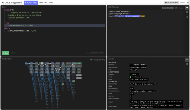
Apart from command-line tooling, the LMQL runtime also includes a web-based playground, helpful in constructing and debugging LMQL programs. A screenshot of the visual debugger is shown in Fig. 14. A hosted version can also be found at https://lmql.ai/playground.
Editor and Compiler
The visual debugger provides an editor window for constructing LMQL queries. After a query is executed, users can view the compiler output, i.e. the resulting python code, including the code that constructs the computational graph and executes the prompt.
Decoder Graph
Users can track the different decoding branches of the currently active decoding method in real-time. This includes simple parallel decoding when sampling more than one sequence, but also multi-branch decoding like beam search. The debugger visualizes (sub-)tokens, and at each decoder step, users can inspect the current interaction trace, the value of prompt variables as well as the current state of where clause validation.
Validation and Masking
Lastly, the computational graph of the where clause can be visualized and users can track the current value of the expression. In addition to the regular value semantics and partial evaluation, this includes support for both Final and Follow semantics. Different shades of green and red indicate final and non-final True and False values, respectively. The FollowMap at each operation can also be inspected, allowing for a detailed analysis of the current state of the computational graph. This can be helpful when developing new LMQL operators, as it allows for a quick and easy debugging of the underlying semantics.