On generalized eigenvalue problems of fractional $(p,q)$-Laplace operator with two parameters

Abstract.

For $s_{1},s_{2}\in(0,1)$ and $p,q\in(1,\infty)$, we study the following nonlinear Dirichlet eigenvalue problem with parameters $\alpha,\beta\in\mathbb{R}$ driven by the sum of two nonlocal operators:

$$(-\Delta)^{s_{1}}_{p}u+(-\Delta)^{s_{2}}_{q}u=\alpha|u|^{p-2}u+\beta|u|^{q-2}u\;\;\text{in }\Omega,\quad u=0\;\;\text{in }\mathbb{R}^{d}\setminus\Omega,\ \ \ \qquad\quad\mathrm{(P)}$$

where $\Omega\subset\mathbb{R}^{d}$ is a bounded open set. Depending on the values of $\alpha,\beta$, we completely describe the existence and non-existence of positive solutions to (P). We construct a continuous threshold curve in the two-dimensional $(\alpha,\beta)$-plane, which separates the regions of the existence and non-existence of positive solutions. In addition, we prove that the first Dirichlet eigenfunctions of the fractional $p$-Laplace and fractional $q$-Laplace operators are linearly independent, which plays an essential role in the formation of the curve. Furthermore, we establish that every nonnegative solution of (P) is globally bounded.

1. Introduction and Main Results

In this paper, we are concerned with the existence and non-existence of positive solutions to the following nonlinear eigenvalue problem involving the fractional $(p,q)$-Laplace operator with zero Dirichlet boundary condition:

$$(-\Delta)^{s_{1}}_{p}u+(-\Delta)^{s_{2}}_{q}u=\alpha|u|^{p-2}u+\beta|u|^{q-2}u\;\;\text{in }\Omega,\quad u=0\;\;\text{in }\mathbb{R}^{d}\setminus\Omega, \alpha,\beta$$ (EV; )

where $0<s_{2}<s_{1}<1<q<p<\infty$, $\alpha,\beta\in\mathbb{R}$ are two parameters and $\Omega\subset\mathbb{R}^{d}$ is a bounded open set. In general, the fractional $r$-Laplacian $(-\Delta)^{s}_{r}$ ($s\in(0,1)$ and $r\in(1,\infty)$) is defined as

$$(-\Delta)^{s}_{r}u(x):=\text{P.V.}\int_{\mathbb{R}^{d}}\frac{|u(x)-u(y)|^{r-2}(u(x)-u(y))}{|x-y|^{d+sr}}\,{\rm d}y,\;\;\;x\in\mathbb{R}^{d},$$

where P.V. stands for the principle value.

The local counterpart of (EV; $\alpha,\beta$) is the following Dirichlet eigenvalue problem for the $(p,q)$-Laplace operator:

$$-\Delta_{p}u-\Delta_{q}u=\alpha|u|^{p-2}u+\beta|u|^{q-2}u\;\;\text{in }\Omega,\quad u=0\;\;\text{in }\partial\Omega.$$ (1.1)

The study of $(p,q)$-Laplace operators are well known for their applications in physics, chemical reactions, reaction-diffusion equations e.t.c. for details, see [15, 19, 21] and the references therein. Some authors considered the eigenvalue problems for the $(p,q)$-Laplace operator. In this direction, for $\alpha=\beta$, Motreanu-Tanaka in [30] obtained the existence and non-existence of positive solutions of (1.1). For $\alpha\neq\beta$, in [8] Bobkov-Tanaka extended this result by providing a certain region in the $(\alpha,\beta)$-plane that allocates the sets of existence and non-existence of positive solutions of (1.1). Moreover, they constructed a threshold curve in the first quadrant of the $(\alpha,\beta)$-plane, which separates these two sets. Later, in [9], the same authors plotted a different curve for the existence of ground states and the multiplicity of the positive solutions for (1.1). It is essential that in which region the positive solution of (1.1) exists or does not exist, and the behaviour of the threshold curve depends on whether $\phi_{p},\phi_{q}$ are linearly independent, where $\phi_{p}\text{ and }\phi_{q}$ are the first Dirichlet eigenfunctions of the operators $-\Delta_{p}$ and $-\Delta_{q}$ respectively. For other results related to the positive solutions of eigenvalue problems involving $(p,q)$-Laplace operator, we refer to [6, 10, 33] and the references therein.

In the nonlocal case, parallelly, many authors studied the nonlinear equations driven by the sum of fractional $p$-Laplace and fractional $q$-Laplace operators with the critical exponent. For example, see [3, 4, 7, 25, 26] where the weak solution’s existence, regularity, multiplicity, positivity and other qualitative properties are investigated. The study of (EV; $\alpha,\beta$) is motivated by the Dancer-Fučik (DF) spectrum of the fractional $r$-Laplace operator. The DF spectrum of the operator $(-\Delta)^{s}_{r}$ is the set of all points $(\alpha,\beta)\in\mathbb{R}^{2}$ such that the following problem

$$(-\Delta)_{r}^{s}u=\alpha(u^{+})^{r-1}-\beta(u^{-})^{r-1}\text{ in }\Omega,\quad u=0\text{ in }\mathbb{R}^{d}\setminus\Omega,$$ (1.2)

admits a nontrivial weak solution, where $u^{\pm}=\max\{\pm u,0\}$ is the positive and negative part of $u$. For $r=2$, in [27], Goyal-Sreenadh considered (1.2) and proved the existence of a first nontrivial curve in the DF spectrum. They also showed that the curve is Lipschitz continuous, strictly decreasing, and studied its asymptotic behaviour. For $r\neq 2$, in [32], the authors constructed an unbounded sequence of decreasing curves in the DF spectrum. Nevertheless, the study of the spectrum for the fractional $(p,q)$-Laplace operator is not well explored. In [31], for $\alpha=\beta$, Nguyen-Vo studied the following weighted eigenvalue problem with zero Dirichlet boundary condition:

$$(-\Delta)^{s_{1}}_{p}u+(-\Delta)^{s_{2}}_{q}u=\alpha\left(m_{p}|u|^{p-2}u+m_{q}|u|^{q-2}u\right)\;\;\text{in }\Omega,\quad u=0\;\;\text{in }\mathbb{R}^{d}\setminus\Omega,$$ (1.3)

where $0<s_{2}<s_{1}<1<q\leq p<\infty$, the weights $m_{p},m_{q}$ are bounded in $\Omega$ and satisfy $m_{p}^{+},m_{q}^{+}\not\equiv 0$. Depending on the values of $\alpha$, the authors obtained the existence and non-existence of positive solutions of (1.3).

The primary aim of this paper can be summarized into the following two aspects:

(a) We provide a comprehensive analysis of the sets in the $(\alpha,\beta)$-plane that determine the existence and non-existence of positive solutions for the equation (EV; $\alpha,\beta$). Following the local case approach, we construct a continuous threshold curve denoted as $\mathcal{C}$ that effectively separates the regions where positive solutions exist from those where they do not. In some specific regions of the $(\alpha,\beta)$-plane, we employ the sub-super solutions technique to establish the existence of positive solutions. To apply this technique, we utilize the crucial result stated in Theorem 4.1, which proves that every nonnegative solution of (EV; $\alpha,\beta$) is globally bounded.

(b) The existence and non-existence of positive solutions to (EV; $\alpha,\beta$) depend on the following statement:

$$\phi_{s_{1},p}\neq c\phi_{s_{2},q}\text{ for any }c\in{\mathbb{R}},$$ (LI)

where $\phi_{s_{1},p}\text{ and }\phi_{s_{2},q}$ are the first eigenfunctions of the operators $(-\Delta)_{p}^{s_{1}}$ and $(-\Delta)_{q}^{s_{2}}$ corresponding to the first eigenvalues $\lambda_{s_{1},p}^{1}$ and $\lambda_{s_{2},q}^{1}$ respectively in $\Omega$ under zero Dirichlet boundary condition. While this linear independence condition for the operators $-\Delta_{p}$ and $-\Delta_{q}$ was conjectured in [8] and later proved in [9], its validity remains unknown for any $s_{1},s_{2}\in(0,1)$. Nevertheless, several authors have assumed the condition (LI) in various contexts (e.g., [24, 31]). We establish the validity of (LI) under certain assumptions on $s_{1}$ and $s_{2}$, as demonstrated in Theorem 1.9.

Recall that, for $0<s<1\leq r<\infty$, the fractional Sobolev space is defined as

$$W^{s,r}(\Omega):=\left\{u\in L^{r}(\Omega):[u]_{s,r,\Omega}<\infty\right\},$$

with the so-called fractional Sobolev norm $\left\lVert u\right\rVert_{s,r,\Omega}:=(\|u\|_{L^{r}(\Omega)}^{r}+[u]_{s,r,\Omega}^{r})^{\frac{1}{r}},$ where

$$[u]_{s,r,\Omega}^{r}:=\iint\limits_{\Omega\times\Omega}\frac{|u(x)-u(y)|^{r}}{|x-y|^{d+sr}}\,{\rm d}x{\rm d}y,$$

is called the Gagliardo seminorm. For $r\in(1,\infty)$, $W^{s,r}(\Omega)$ is a reflexive Banach space with respect to the fractional Sobolev norm $\left\lVert\cdot\right\rVert_{s,r,\Omega}$. Now we consider the following closed subspace of $W^{s,r}(\mathbb{R}^{d})$:

$$W_{0}^{s,r}(\Omega):=\{u\in W^{s,r}(\mathbb{R}^{d}):u=0\text{ in }\mathbb{R}^{d}\setminus\Omega\},$$

endowed with the seminorm $[\cdot]_{s,r,\mathbb{R}^{d}}$, which is an equivalent norm in $W_{0}^{s,r}(\Omega)$ ([12, Lemma 2.4]). For details of the fractional Sobolev spaces and their related embedding results, we refer to [12, 14, 20] and the references therein. For $s_{1}>s_{2}$ and $p>q\geq 1$, the continuous embedding ${W_{0}^{s_{1},p}(\Omega)}\hookrightarrow{W_{0}^{s_{2},q}(\Omega)}$ (see [5, Proposition 2.2]) allows us to introduce the notion of weak solution for (EV; $\alpha,\beta$) in the following sense:

Definition 1.1.

A function $u\in{W_{0}^{s_{1},p}(\Omega)}$ is called a weak solution of (EV; $\alpha,\beta$) if the following identity holds for all $\phi\in{W_{0}^{s_{1},p}(\Omega)}$:

$$\iint\limits_{\mathbb{R}^{d}\times\mathbb{R}^{d}}\frac{|u(x)-u(y)|^{p-2}(u(x)-u(y))(\phi(x)-\phi(y))}{|x-y|^{d+s_{1}p}}\,{\rm d}x{\rm d}y\\ +\iint\limits_{\mathbb{R}^{d}\times\mathbb{R}^{d}}\frac{|u(x)-u(y)|^{q-2}(u(x)-u(y))(\phi(x)-\phi(y))}{|x-y|^{d+s_{2}q}}\,{\rm d}x{\rm d}y=\alpha\displaystyle{\int_{\Omega}}|u|^{p-2}u\phi\,{\rm d}x+\beta\displaystyle{\int_{\Omega}}|u|^{q-2}u\phi\,{\rm d}x.$$

In our first theorem, we prove the existence of a positive solution for (EV; $\alpha,\beta$) if any of $\alpha$ and $\beta$ is larger than the first Dirichlet eigenvalue of the fractional $p$-Laplacian and fractional $q$-Laplacian respectively. We also show that this range of $\alpha,\beta$ is necessary for the existence of a positive solution when (LI) does not hold.

Theorem 1.2.

Let $0<s_{2}<s_{1}<1<q<p<\infty$. Assume that

$$(\alpha,\beta)\in\left((\lambda_{s_{1},p}^{1},\infty)\times(-\infty,\lambda_{s_{2},q}^{1})\right)\cup\left((-\infty,\lambda_{s_{1},p}^{1})\times(\lambda_{s_{2},q}^{1},\infty)\right)\cup\left(\{\lambda_{s_{1},p}^{1}\}\times\{\lambda_{s_{2},q}^{1}\}\right).$$ (1.4)

The following hold (see Figure 1):

• (Sufficient condition): Let $\alpha,\beta$ satisfy (1.4). In the case, when $\alpha=\lambda_{s_{1},p}^{1}$ and $\beta=\lambda_{s_{2},q}^{1}$, we assume that (LI) violates. Then (EV; $\alpha,\beta$) admits a positive solution.

• (Necessary condition): Let (LI) violates and (EV; $\alpha,\beta$) admits a positive solution. Then $\alpha,\beta$ satisfy (1.4).

Remark 1.3.

(i) The above theorem asserts that (EV; $\lambda_{s_{1},p}^{1},\,\lambda_{s_{2},q}^{1}$) admits a positive solution if and only if (LI) violates. Indeed, (EV; $\lambda_{s_{1},p}^{1},\,\lambda_{s_{2},q}^{1}$) admits a non-trivial solution only when (LI) violates (see Proposition 6.1).

(ii) If (LI) violates, then Theorem 1.2 gives a complete description of the set of existence and non-existence of positive solutions of (EV; $\alpha,\beta$). In particular, Theorem 1.2 generalizes the result of [31, Theorem 1.1] for $\alpha\neq\beta$.

It is observed that for $\alpha,\beta\in\mathbb{R}$, the problem (EV; $\alpha,\beta$) is equivalent to the problem (EV; $\beta+\theta,\beta$), where $\theta=\alpha-\beta.$ Using this terminology we define the following curve:

Definition 1.4 (Threshold curve).

For brevity, denote $\beta=\lambda$. For each $\theta\in\mathbb{R}$ consider the following quantity:

$$\lambda^{*}(\theta):=\sup\left\{\lambda\in\mathbb{R}:({\color[rgb]{0,0,1}\text{EV; $\lambda+\theta,\lambda$}})\text{ has a positive solution}\right\}.$$ (1.5)

If such $\lambda$ does not exist, we then set $\lambda^{*}(\theta)=-\infty.$ The threshold curve corresponding to (EV; $\alpha,\beta$) is defined as $\mathcal{C}:=\{(\lambda^{*}(\theta)+\theta,\lambda^{*}(\theta)):\theta\in{\mathbb{R}}\}$. Also, we define the following quantities:

$$\theta^{*}:=\lambda^{1}_{s_{1},p}-\lambda^{1}_{s_{2},q},\,\alpha^{*}_{s_{1},p}:=\frac{[\phi_{s_{2},q}]_{s_{1},p,\mathbb{R}^{d}}^{p}}{\left\lVert\phi_{s_{2},q}\right\rVert_{L^{p}(\Omega)}^{p}},\text{ and }\theta^{*}_{+}:=\alpha^{*}_{s_{1},p}-\lambda^{1}_{s_{2},q}.$$

Clearly, $\theta^{*}\leq\theta^{*}_{+}$ and $\theta^{*}=\theta^{*}_{+}$ if and only if (LI) violates (from (iv) of Proposition 2.1).

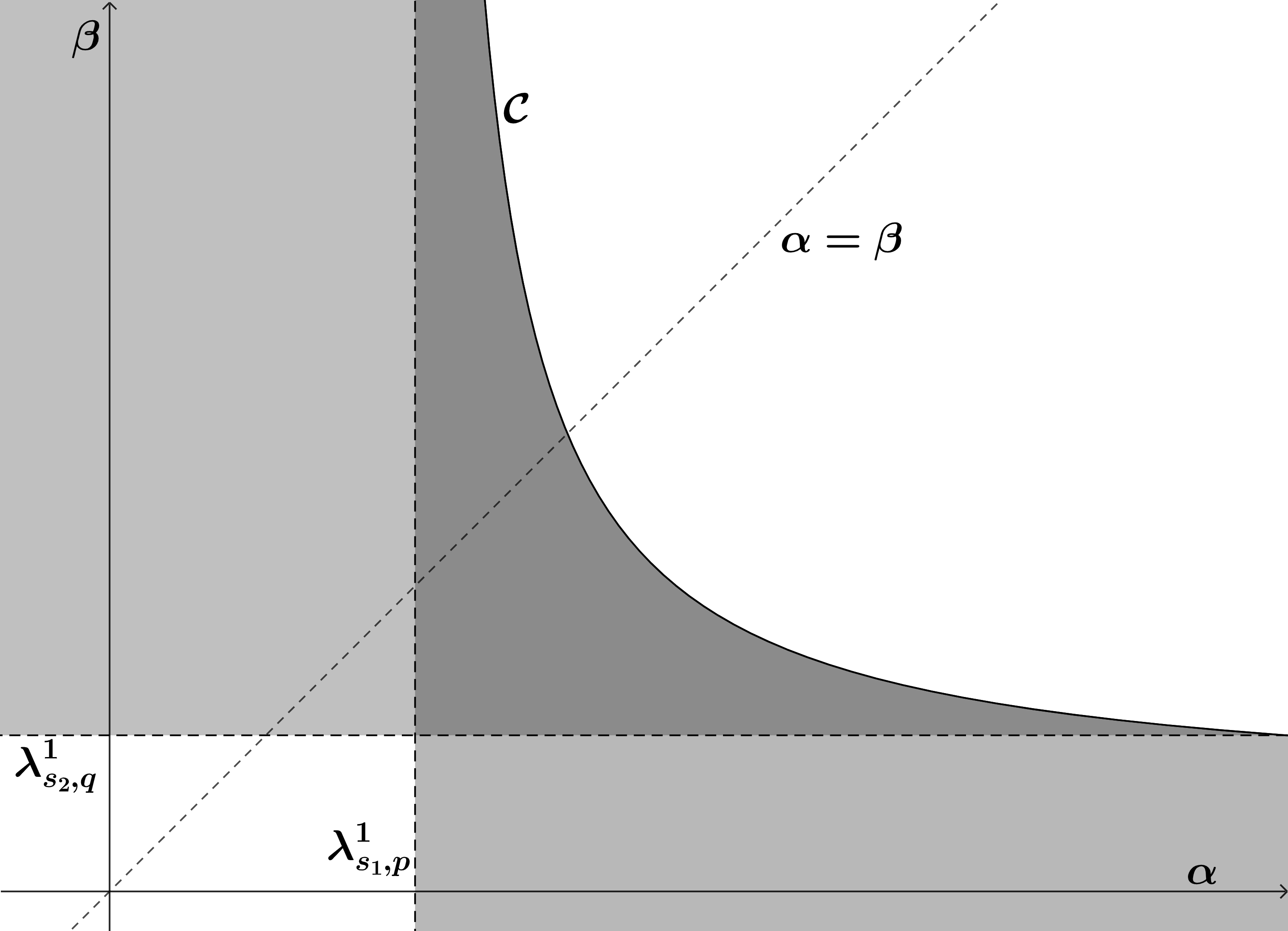
(a) The case (LI) holds (with $\alpha^{*}_{s_{1},p}<\infty$)

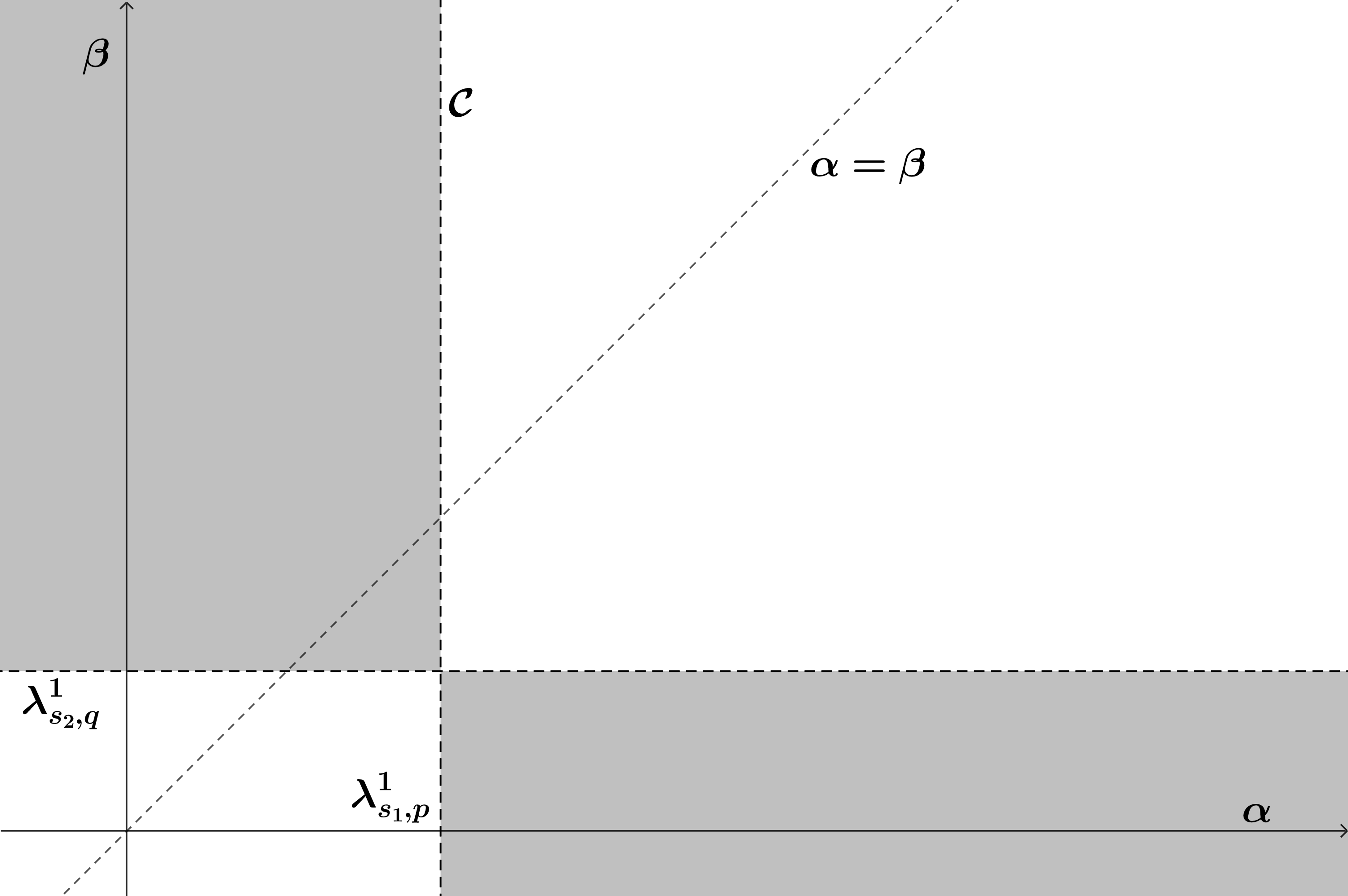
(b) The case (LI) does not hold

Figure 1. Shaded region denotes existence, and unshaded region denotes non-existence of positive solutions.

In the following proposition, we discuss some qualitative properties of $\mathcal{C}$ and see that $\mathcal{C}$ carries similar behaviours as in the local case [8, Proposition 3 and Fig. 2].

Proposition 1.5.

Let $0<s_{2}<s_{1}<1<q<p<\infty$. Then the following hold:

• $\lambda^{*}(\theta)<\infty$ for all $\theta\in\mathbb{R}$.

• $\lambda^{*}(\theta^{*})+\theta^{*}>\lambda^{1}_{s_{1},p}$ and $\lambda^{*}(\theta^{*})>\lambda^{1}_{s_{2},q}$ if and only if (LI) holds.

• $\lambda^{*}(\theta)+\theta\geq\lambda^{1}_{s_{1},p}$ and $\lambda^{*}(\theta)\geq\lambda^{1}_{s_{2},q}$ for all $\theta\in\mathbb{R}.$

• $\lambda^{*}(\theta)$ is decreasing and $\lambda^{*}(\theta)+\theta$ is increasing on $\mathbb{R}.$

• If $\alpha^{*}_{s_{1},p}$ is finite, then $\lambda^{*}(\theta)=\lambda^{1}_{s_{2},q}$ for all $\theta\geq\theta^{*}_{+}.$

• $\lambda^{*}$ is continuous on $\mathbb{R}.$

According to (iii) of the above proposition, $\mathcal{C}\subset([\lambda_{s_{1},p}^{1},\infty)\times[\lambda_{s_{2},q}^{1},\infty))$. Further, if $\alpha^{*}_{s_{1},p}=\infty$, from the property (iii), we observe that $\mathcal{C}$ always lies above the line $\beta=\lambda_{s_{2},q}^{1}$. From now onwards, we assume that $\alpha^{*}_{s_{1},p}<\infty$. In the following theorem, we demonstrate that $\mathcal{C}$ separates the sets of existence and non-existence of positive solutions in the region $([\lambda_{s_{1},p}^{1},\infty)\times[\lambda_{s_{2},q}^{1},\infty))$ (see Figure 1).

Theorem 1.6.

Let $0<s_{2}<s_{1}<1<q<p<\infty$. Let $\alpha\geq\lambda_{s_{1},p}^{1}$ and $\beta\geq\lambda_{s_{2},q}^{1}$. Assume that (LI) holds.

• If $\beta\in(\lambda_{s_{2},q}^{1},\lambda^{*}(\theta))$, then (EV; $\alpha,\beta$) admits a positive solution.

• If $\alpha>\lambda_{s_{1},p}^{1}$ and $\beta<\lambda^{*}(\theta)$, then (EV; $\alpha,\beta$) admits a positive solution.

• If $\beta>\lambda^{*}(\theta)$, then there does not exist any positive solution for (EV; $\alpha,\beta$).

Now we state the existence and non-existence of positive solutions on the curve $\mathcal{C}$ (see Figure 1).

Theorem 1.7.

Let $0<s_{2}<s_{1}<1<q<p<\infty$.

1. If $\theta<\theta^{*}_{+}$, then (EV; $\lambda^{*}(\theta)+\theta,\lambda^{*}(\theta)$) admits a positive solution.

2. If $\theta>\theta^{*}_{+}$, then there does not exist any positive solution for (EV; $\lambda^{*}(\theta)+\theta,\lambda^{*}(\theta)$).

The above theorem does not consider the borderline case $\theta=\theta_{+}^{*}$. In this case, we have a partial result in Remark 6.9, which says that (EV; $\lambda^{*}(\theta)+\theta,\lambda^{*}(\theta)$) does not admit any ground state solution.

Remark 1.8.

The relations among $s_{1},s_{2},p,q$ are taken without loss of any generality. All the preceding results in this paper hold for the remaining cases by choosing the appropriate solution space as given below:

1. For $s_{1}<s_{2}$ and $p<q$ (symmetric), we choose the solution space as ${W_{0}^{s_{2},q}(\Omega)}$.

2. For $s_{2}<s_{1}$ and $p<q$ (cross), we choose the solution space as ${W_{0}^{s_{1},p}(\Omega)}\cap{W_{0}^{s_{2},q}(\Omega)}$ endowed with the norm $[\cdot]_{s_{1},p,\mathbb{R}^{d}}+[\cdot]_{s_{2},q,\mathbb{R}^{d}}$.

3. For $s_{1}=s_{2}=s$ and $p\neq q$, we choose the solution space as $W^{s,p}_{0}(\Omega)\cap W^{s,q}_{0}(\Omega)$ endowed with the norm $[\cdot]_{s,p,\mathbb{R}^{d}}+[\cdot]_{s,q,\mathbb{R}^{d}}$.

The next theorem verifies the linear independency of the first Dirichlet eigenfunctions of the fractional $p$-Laplacian and the fractional $q$-Laplacian.

Theorem 1.9.

Let $1<q<p<\infty$ and $s_{1},s_{2}\in(0,1)$ satisfy the following condition:

$$\frac{s_{1}{p^{\prime}}}{{q^{\prime}}}<s_{2}<s_{1}.$$

Then the set $\{\phi_{s_{1},p},\phi_{s_{2},q}\}$ is linearly independent.

Remark 1.10.

Theorem 1.9 holds if we take the other relations among $s_{1},s_{2},p,q$ listed below:

1. For $1<p<q<\infty$ and $\frac{s_{2}{q^{\prime}}}{{p^{\prime}}}<s_{1}<s_{2}$ (interchanging the roles of $s_{1},s_{2},p,q$).

2. For $1<q<p<\infty$ and $s_{1}=s_{2}$.

The rest of the paper is organized as follows. Section 2 briefly discusses the first Dirichlet eigenpair of fractional $r$-Laplace operator, recalls the discrete Picone’s inequalities, and proves some technical results. In Section 3, we prove the validity of (LI). This section contains the proof of Theorem 1.9. In Section 4, we establish the regularity of the solution for (EV; $\alpha,\beta$) and state a version of the strong maximum principle related to (EV; $\alpha,\beta$). Section 5 studies various frameworks of energy functionals associated with (EV; $\alpha,\beta$). Finally, Section 6 studies the existence and non-existence of positive solutions for (EV; $\alpha,\beta$). In this section, we prove Theorem 1.2-1.7 and Proposition 1.5.

2. Preliminaries

In this section, we recall some qualitative properties of the first nonlocal eigenvalue and its corresponding eigenfunction. Afterwards, we recall the discrete Picone’s identities. We list the following notations to be used in this paper:

Notation:

• $B_{R}(x)\subset\mathbb{R}^{d}$ denotes an open ball of radius $R>0$ centered at $x.$

• For a set $E\subset\mathbb{R}^{d}$, $|E|$ denotes the Lebesgue measure of $E$.

• We denote ${\rm d}\mu_{1}:=\lvert x-y\rvert^{-(d+s_{1}p)}{\rm d}x{\rm d}y$ and ${\rm d}\mu_{2}:=\lvert x-y\rvert^{-(d+s_{2}q)}{\rm d}x{\rm d}y$.

• For $r\in(1,\infty)$, the conjugate of $r$ is denoted as $r^{\prime}:=\frac{r}{r-1}$.

• For $0<s<1<r<\infty$, we denote $[\cdot]_{s,r,\mathbb{R}^{d}}$ as $[\cdot]_{s,r}$, and $\left\lVert\cdot\right\rVert_{L^{r}(\Omega)}$ as $\left\lVert\cdot\right\rVert_{r}$.

• For $k\in\mathbb{N}$, we denote $u_{k}(x):=u(x)+\frac{1}{k}$ where $x\in\mathbb{R}^{d}$.

• For $\gamma\in(0,1)$, the Hölder seminorm $[f]_{C^{0,\gamma}(\Omega)}:=\underset{x,y\in\Omega,\,x\neq y}{\sup}\displaystyle\frac{\lvert f(x)-f(y)\rvert}{\lvert x-y\rvert^{\gamma}}$.

• For $sr<d$ (where $0<s<1<r<\infty$), the fractional critical exponent $\displaystyle r^{*}_{s}:=\frac{rd}{d-sr}$.

• For each $n\in\mathbb{N}$, we denote the positive and negative parts $(f_{n})^{\pm}$ by $f_{n}^{\pm}:=\max\{\pm f_{n},0\}$.

• Eigenvalue of (2.1), $\lambda_{s,r}(\Omega)$ is denoted as $\lambda_{s,r}$.

• We denote the eigenfunction of (2.1) corresponding to the first eigenvalue $\lambda^{1}_{s,r}$ as $\phi_{s,r}$.

• For $r\in(1,\infty)$, $x_{0}\in\Omega$ and $R>0$, the nonlocal tail of $f\in W^{s,r}_{0}(\Omega)$ is defined as

  $$\mathrm{Tail}_{r}(f;x_{0},R):=\left(R^{sr}\int_{\mathbb{R}^{d}\setminus B_{R}(x_{0})}\frac{|f(x)|^{r-1}}{|x-x_{0}|^{d+sr}}\,{\rm d}x\right)^{\frac{1}{r-1}}.$$

• $C$ is denoted as a generic positive constant.

2.1. First eigenvalue of fractional $r$-Laplacian

For a bounded open set $\Omega\subset\mathbb{R}^{d}$ and $0<s<1<r<\infty$, we consider the following nonlinear eigenvalue problem:

$$(-\Delta)_{r}^{s}u=\lambda_{s,r}|u|^{r-2}u\;\text{in }\Omega,\quad u=0\;\text{ in }\mathbb{R}^{d}\setminus\Omega.$$ (2.1)

We say $\lambda_{s,r}$ is an eigenvalue of (2.1), if there exists non-zero $u\in{W_{0}^{s,r}(\Omega)}$ satisfying the following identity for all $\phi\in{W_{0}^{s,r}(\Omega)}$:

$$\begin{split}\iint\limits_{\mathbb{R}^{d}\times\mathbb{R}^{d}}\frac{|u(x)-u(y)|^{r-2}(u(x)-u(y))(\phi(x)-\phi(y))}{|x-y|^{d+sr}}\,{\rm d}x{\rm d}y=\lambda_{s,r}\displaystyle{\int_{\Omega}}|u(x)|^{r-2}u(x)\phi(x)\,{\rm d}x.\end{split}$$

In this case, $u$ is called an eigenfunction corresponding to $\lambda_{s,r}$, and we denote $\left(\lambda_{s,r},u\right)$ as an eigenpair. In the following proposition, we collect some qualitative properties of the first eigenpair of (2.1).

Proposition 2.1.

For $r\in(1,\infty)$ and $s\in(0,1)$, consider the following quantity:

$$\lambda^{1}_{s,r}=\inf\left\{[u]_{s,r}^{r}:u\in{W_{0}^{s,r}(\Omega)}\text{ and }\displaystyle{\int_{\Omega}}|u|^{r}=1\right\}.$$

Then the following hold:

• $\lambda^{1}_{s,r}$ is the first positive eigenvalue of (2.1).

• Every eigenfunction corresponding to $\lambda^{1}_{s,r}$ has a constant sign in $\Omega$.

• If $v$ is an eigenfunction of (2.1) corresponding to an eigenvalue $\lambda_{s,r}>0$ such that $v>0$ a.e. in $\Omega$, then $\lambda_{s,r}=\lambda^{1}_{s,r}$.

• Any two eigenfunctions corresponding to $\lambda^{1}_{s,r}$ are constant multiple of each other.

• Any eigenfunction of (2.1) corresponding to an eigenvalue $\lambda_{s,r}$ is in $L^{\sigma}(\mathbb{R}^{d})$ for every $\sigma\in[1,\infty]$. Moreover, if $\Omega$ is of class $\mathcal{C}^{1,1}$, then the eigenfunction lies in $C^{0,\gamma}(\overline{\Omega})$ for some $\gamma\in(0,s]$.

Proof.

For proof of (i) and (iii), we refer to [22, Lemma 2.1 and Theorem 4.1]. For (ii), see [14, Proposition 2.6]. Then the proof of (iv) follows using [22, Theorem 4.2].

(v) Let $u$ be an eigenfunction of (2.1) corresponding to $\lambda_{s,r}$. By [12, Theorem 3.3], $u\in L^{\infty}(\mathbb{R}^{d})$. Further, since $u\in W^{s,r}(\mathbb{R}^{d})\cap L^{\infty}(\mathbb{R}^{d})$, the interpolation argument yields $u\in L^{\sigma}(\mathbb{R}^{d})$ for every $\sigma\geq r$. Also for $\sigma\in[1,r)$, applying Hölder’s inequality with the conjugate pair $(\frac{r}{\sigma},\frac{r-\sigma}{\sigma})$,

$$\int_{\Omega}\lvert u\rvert^{\sigma}\leq\left(\int_{\Omega}\lvert u\rvert^{r}\right)^{\frac{\sigma}{r}}\lvert\Omega\rvert^{\frac{r-\sigma}{r}}.$$

Thus, $u\in L^{\sigma}(\mathbb{R}^{d})$ for every $\sigma\in[1,\infty]$. Furthermore, we apply [28, Theorem 1.1] to get $u\in C^{0,\gamma}(\overline{\Omega})$ for some $\gamma\in(0,s]$. ∎

2.2. Some important results

In this subsection, we state some elementary inequalities, recall Picone’s inequalities for nonlocal operators and collect some test functions in $W^{s,r}_{0}(\Omega)$.

Lemma 2.2.

Let $a,b\in{\mathbb{R}}$, and $\gamma\in{\mathbb{R}}^{+}$. The following hold:

1. If $\gamma>1$, then

   $$\lvert a-b\rvert^{\gamma-2}(a-b)(a^{+}-b^{+})\geq\lvert a^{+}-b^{+}\rvert^{\gamma};\quad\lvert a-b\rvert^{\gamma-2}(a-b)(b^{-}-a^{-})\geq\lvert a^{-}-b^{-}\rvert^{\gamma},$$

   where $a^{\pm}=\max\{\pm a,0\}$.

2. If $\gamma\geq 2$, then $\lvert a-b\rvert^{\gamma-2}(a-b)\leq C\left(\lvert a\rvert^{\gamma-2}a-\lvert b\rvert^{\gamma-2}b\right)$ for some $C=C(\gamma)>0$.

3. $\lvert\lvert a\rvert^{\gamma}-\lvert b\rvert^{\gamma}\rvert\leq\gamma\left(\lvert a\rvert^{\gamma-1}+\lvert b\rvert^{\gamma-1}\right)\lvert a-b\rvert$.

Proof.

Proof of (i) follows from [14, Lemma A.2]. Proof of (ii) follows from [29, (2.2) of Page 5]. Proof of (iii) follows using the fundamental theorem of calculus. ∎

We recall several versions of the discrete Picone’s inequality that are useful in proving our results.

Lemma 2.3 (Discrete Picone’s inequality).

Let $r_{1},r_{2}\in(1,\infty)$ with $r_{2}\leq r_{1}$ and let $f,g:\mathbb{R}^{d}\to\mathbb{R}$ be two measurable functions with $f>0,\;g\geq 0$. Then the following hold:

1. For $x,y\in\mathbb{R}^{d}$,

   $$|f(x)-f(y)|^{r_{1}-2}(f(x)-f(y))\left(\frac{g(x)^{r_{2}}}{f(x)^{r_{2}-1}}-\frac{g(y)^{r_{2}}}{f(y)^{r_{2}-1}}\right)\leq\lvert g(x)-g(y)\rvert^{r_{2}}\lvert f(x)-f(y)\rvert^{r_{1}-r_{2}}.$$

2. For $x,y\in\mathbb{R}^{d}$,

   $$|f(x)-f(y)|^{r_{2}-2}(f(x)-f(y)) \left(\frac{g(x)^{r_{1}}}{f(x)^{r_{1}-1}}-\frac{g(y)^{r_{1}}}{f(y)^{r_{1}-1}}\right)$$

   $$\leq|g(x)-g(y)|^{r_{2}-2}(g(x)-g(y))\left(\frac{g(x)^{r_{1}-r_{2}+1}}{f(x)^{r_{1}-r_{2}}}-\frac{g(y)^{r_{1}-r_{2}+1}}{f(y)^{r_{1}-r_{2}}}\right).$$

3. Let $\alpha,\beta\geq 1$. Then for $x,y\in\mathbb{R}^{d}$,

   $$|f(x)-f(y)|^{r_{1}-2}(f(x)-f(y)) \left(\frac{g(x)^{r_{1}}}{\alpha f(x)^{r_{1}-1}+\beta f(x)^{r_{2}-1}}-\frac{g(y)^{r_{1}}}{\alpha f(y)^{r_{1}-1}+\beta f(y)^{r_{2}-1}}\right)$$

   $$\leq\lvert g(x)-g(y)\rvert^{r_{1}}.$$

4. Let $\alpha,\beta\geq 1$. Then for $x,y\in\mathbb{R}^{d}$,

   $$|f(x)-f(y)|^{r_{2}-2}(f(x)-f(y)) \left(\frac{g(x)^{r_{1}}}{\alpha f(x)^{r_{1}-1}+\beta f(x)^{r_{2}-1}}-\frac{g(y)^{r_{1}}}{\alpha f(y)^{r_{1}-1}+\beta f(y)^{r_{2}-1}}\right)$$

   $$\leq\lvert f(x)^{\frac{r_{1}}{r_{2}}}-f(y)^{\frac{r_{1}}{r_{2}}}\rvert^{r_{2}}.$$

Moreover, the equality holds in the above inequalities if and only if $f=cg$ a.e. in $\mathbb{R}^{d}$ for some $c\in{\mathbb{R}}$.

Proof.

For the proof of (i), see [11, Proposition 4.2]. Proof of (ii), (iii), and (iv) follows from [24, Theorem 2.3 and Remark 2.6]. ∎

The following lemma verifies that certain functions are in the fractional Sobolev space, which we require in the subsequent sections.

Lemma 2.4.

Let $s\in(0,1)$ and $r_{1},r_{2}\in(1,\infty)$. Let $u\in W^{s,r_{1}}_{0}(\Omega)$ be a non-negative function. For $v\in W^{s,r_{1}}_{0}(\Omega)\cap L^{\infty}(\Omega)$, the following functions

$$\phi_{k}:=\frac{|v|^{r_{1}}}{u_{k}^{r_{1}-1}+u_{k}^{r_{2}-1}},\,\psi_{k}:=\frac{|v|^{r_{1}}}{u_{k}^{r_{2}-1}},\,\text{ and }\,\eta_{k}:=\frac{|v|^{r_{1}-r_{2}+1}}{u_{k}^{r_{1}-r_{2}}}\text{with }r_{2}<r_{1}$$

lie in $W^{s,r_{1}}_{0}(\Omega)$.

Proof.

We only prove that $\phi_{k}\in W^{s,r_{1}}_{0}(\Omega)$. For other functions, the proof follows using similar arguments. Clearly, $\phi_{k}$ is in $L^{r}_{1}(\Omega)$ and $\phi_{k}=0$ in $\Omega^{c}$, for every $k.$ Next, claim that $[\phi_{k}]_{s,r_{1}}<\infty$. In order to show this, for $x,\,y\in\mathbb{R}^{d}$, we calculate

$$|\phi_{k}(x)-\phi_{k}(y)|$$

$$=\left|\frac{|v(x)|^{r_{1}}}{u_{k}(x)^{r_{1}-1}+u_{k}(x)^{r_{2}-1}}-\frac{|v(y)|^{r_{1}}}{u_{k}(y)^{r_{1}-1}+u_{k}(y)^{r_{2}-1}}\right|$$

$$=\left|\frac{|v(x)|^{r_{1}}-|v(y)|^{r_{1}}}{u_{k}(x)^{r_{1}-1}+u_{k}(x)^{r_{2}-1}}+\frac{|v(y)|^{r_{1}}\left(u_{k}(y)^{r_{1}-1}+u_{k}(y)^{r_{2}-1}-(u_{k}(x)^{r_{1}-1}+u_{k}(x)^{r_{2}-1}\right)}{\left(u_{k}(x)^{r_{1}-1}+u_{k}(x)^{r_{2}-1}\right)\left(u_{k}(y)^{r_{1}-1}+u_{k}(y)^{r_{2}-1}\right)}\right|$$

$$\leq\left(k^{r_{1}-1}+k^{r_{2}-1}\right)\left||v(x)|^{r_{1}}-|v(y)|^{r_{1}}\right|$$

$$\quad+\left\lVert v\right\rVert^{r_{1}}_{\infty}\frac{\left|u_{k}(y)^{r_{1}-1}-u_{k}(x)^{r_{1}-1}\right|+\left|u_{k}(y)^{r_{2}-1}-u_{k}(x)^{r_{2}-1}\right|}{\left(u_{k}(x)^{r_{1}-1}+u_{k}(x)^{r_{2}-1}\right)\left(u_{k}(y)^{r_{1}-1}+u_{k}(y)^{r_{2}-1}\right)}.$$

Using (iii) of Lemma 2.2, we get

$$\begin{split}|\phi_{k}(x)-\phi_{k}(y)|&\leq r_{1}\left(k^{r_{1}-1}+k^{r_{2}-1}\right)\left(|v(x)|^{r_{1}-1}+|v(y)|^{r_{1}-1}\right)|v(x)-v(y)|\\ &\quad+(r_{1}-1)\left\lVert v\right\rVert^{r_{1}}_{\infty}\frac{\left(u_{k}(x)^{r_{1}-2}+u_{k}(y)^{r_{1}-2}\right)}{u_{k}(x)^{r_{1}-1}u_{k}(y)^{r_{1}-1}}|u_{k}(x)-u_{k}(y)|\\ &\quad+(r_{2}-1)\left\lVert v\right\rVert^{r_{1}}_{\infty}\frac{\left(u_{k}(x)^{r_{2}-2}+u_{k}(y)^{r_{2}-2}\right)}{u_{k}(x)^{r_{2}-1}u_{k}(y)^{r_{2}-1}}|u_{k}(x)-u_{k}(y)|.\end{split}$$

Now using $u_{k}^{-1}\leq k$ and $v\in L^{\infty}(\Omega)$, there exists $C=C(r_{1},r_{2},k,\left\lVert v\right\rVert_{\infty})$ such that

$$|\phi_{k}(x)-\phi_{k}(y)| \leq C\left(|v(x)-v(y)|+|u_{k}(x)-u_{k}(y)|\right)=C\left(|v(x)-v(y)|+|u(x)-u(y)|\right).$$

Therefore, $\phi_{k}\in W^{s,r_{1}}_{0}(\Omega)$ follows as $[v]_{s,r_{1}},\,[u]_{s,r_{1}}<\infty.$ This completes the proof. ∎

3. Linear independence of the first eigenfunctions

This section is devoted to proving the linear independency of the first Dirichlet eigenfunctions of the fractional $p$-Laplacian and the fractional $q$-Laplacian. Throughout the section, we assume that $\Omega\subset\mathbb{R}^{d}$ is a bounded open set of class $\mathcal{C}^{1,1}$. For brevity, we denote the first eigenpair of (2.1) by $(\lambda^{1}_{s,r},u)$. From Proposition 2.1, $u>0$ in $\Omega$, $u=0$ in $\mathbb{R}^{d}\setminus\Omega$ and $u\in C(\overline{\Omega})$. Therefore, $u$ attains its maximum in ${\Omega}$. Due to the translation invariance of the fractional $r$-Laplacian, we assume that $\Omega$ contains the origin and the maximum point for $u$ is the origin. Now for $\tau>0$, we consider $\Omega_{\tau}:=\{z\in\mathbb{R}^{d}:\tau z\in\Omega\}$ and define $u_{\tau}:\mathbb{R}^{d}\rightarrow{\mathbb{R}}$ as follows:

$$u_{\tau}(x):=\left\{\begin{array}[]{ll}\frac{u(0)-u(\tau x)}{\tau^{sr^{\prime}}},&\text{for }x\in\Omega_{\tau};\\ \frac{u(0)}{\tau^{sr^{\prime}}},&\text{for }\;x\in\mathbb{R}^{d}\setminus\Omega_{\tau}.\\ \end{array}\right.$$

The following result demonstrates a property of the above function, which plays an essential role in proving (LI).

Lemma 3.1 (Blow-up lemma).

Let $r\in(1,\infty)$ and $s\in(0,1)$. If $\tau_{n}\to 0$, as $n\to\infty$, then there exists a subsequence denoted by $(\tau_{n})$ such that $u_{\tau_{n}}\to\tilde{u}$ in ${\mathcal{C}}_{\text{loc}}(\mathbb{R}^{d})$ as $n\to\infty$. Moreover, $\tilde{u}\in W^{s,r}_{\text{loc}}(\mathbb{R}^{d})\cap{\mathcal{C}}(\mathbb{R}^{d})$ is non-negative, and satisfies the following equation weakly:

$$(-\Delta)^{s}_{r}v=-\lambda^{1}_{s,r}u(0)^{r-1}\text{ in }\mathbb{R}^{d},$$ (3.1)

and $\tilde{u}(0)=0.$

Proof.

Note that for any $\tau>0$, $u_{\tau}\geq 0$, since $u(0)$ is the maximum value for $u$ in $\overline{\Omega}$. Using the fact that $(\lambda^{1}_{s,r},u(\tau x))$ is the first eigenpair for fractional $r$-Laplacian on $\Omega_{\tau}$, we obtain that the following equation holds weakly:

$$(-\Delta)^{s}_{r}u_{\tau}(x)=-(-\Delta)^{s}_{r}u(\tau x)=-\lambda^{1}_{s,r}u(\tau x)^{r-1}\text{ in }\Omega_{\tau},\quad u_{\tau}=\frac{u(0)}{\tau^{sr^{\prime}}}\text{ in }\mathbb{R}^{d}\setminus\Omega_{\tau}.$$ (3.2)

For each $\tau>0$, using Proposition 2.1 and [14, Theorem 3.13], we get $u_{\tau}\in{\mathcal{C}}(\Omega_{\tau})$. Now we divide our proof into two steps. In the first step, we show that $u_{\tau_{n}}\to\tilde{u}$ in $C_{\text{loc}}(\mathbb{R}^{d})$ as $n\to\infty$. In the second step, we prove $\tilde{u}$ is a weak solution to (3.1).

Step 1: Take a ball $B_{R}(0)$ such that $\overline{B_{4R}(0)}\subset\Omega_{\tau}$. We choose $\sigma_{1}>0$ as follows

$$\sigma_{1}:=\frac{d\gamma}{s},\text{ where }\gamma>1.$$

By the nonlocal Harnack inequality (see [25, Theorem 2.2]), there exists $C=C(d,s,r)$ such that

$$\max_{\begin{subarray}{c}B_{R}(0)\end{subarray}}u_{\tau}\leq C\left(\min_{\begin{subarray}{c}B_{2R}(0)\end{subarray}}u_{\tau}+\left\lVert\lambda^{1}_{s,r}\,u^{r-1}\right\rVert_{L^{\sigma_{1}}(B_{2R}(0))}^{\frac{1}{r-1}}\right)=C\left\lVert\lambda^{1}_{s,r}\,u^{r-1}\right\rVert_{L^{\sigma_{1}}(B_{2R}(0))}^{\frac{1}{r-1}},$$ (3.3)

In (3.3) the last equality follows from the fact $\min_{\begin{subarray}{c}B_{2R}(0)\end{subarray}}u_{\tau}=0$, because origin is the maximum point of $u$ in $\Omega$. Further, for $r\geq 2$ we immediately get $(r-1)\sigma_{1}>1$, and for $1<r<2$ we choose

$$\gamma>\left\{\begin{array}[]{ll}\text{max}\left\{\frac{sr}{dr+2(sr-d)},1\right\},&\text{if }sr<d;\\ \text{max}\left\{\frac{s}{d(r-1)},1\right\},&\text{if}\;sr\geq d,\\ \end{array}\right.$$

to get $(r-1)\sigma_{1}>1$. Then Proposition 2.1-(v) and (3.3) yield

$$\max_{\begin{subarray}{c}B_{R}(0)\end{subarray}}u_{\tau}\leq C\left\lVert\lambda^{1}_{s,r}\,u^{r-1}\right\rVert_{L^{\sigma_{1}}(\mathbb{R}^{d})}^{\frac{1}{r-1}}\leq C,$$ (3.4)

where $C=C(d,s,r,\lambda^{1}_{s,r},\left\lVert u\right\rVert_{L^{(r-1)\sigma_{1}}(\mathbb{R}^{d})})$. Next, we define the following exponent

$$\Theta(d,s,r,\sigma_{1}):=\min\left\{\frac{1}{r-1}\left(sr-\frac{d}{\sigma_{1}}\right),1\right\}.\,$$ (3.5)

Then, applying the regularity estimate [13, Theorem 1.4] when $r\geq 2$ and [23, Theorem 1.2] when $1<r<2$, for the problem (3.2) we get the following Hölder regularity estimate of the weak solution $u_{\tau}$ for any $s<\delta<\Theta(d,s,r,\sigma_{1})$:

$$\begin{split}[u_{\tau}]_{C^{0,\delta}(B_{R/8}(0))}&\leq\frac{C}{R^{\delta}}\left[\max_{\begin{subarray}{c}B_{R}(0)\end{subarray}}u_{\tau}+\mathrm{Tail}_{r}(u_{\tau};0,R)+\left(R^{sr-\frac{d}{\sigma_{1}}}\lambda^{1}_{s,r}\left\lVert u^{r-1}\right\rVert_{L^{\sigma_{1}}(B_{R}(0))}\right)^{\frac{1}{r-1}}\right]\\ &:=\frac{C}{R^{\delta}}\left[\max_{\begin{subarray}{c}B_{R}(0)\end{subarray}}u_{\tau}+I_{1}+I_{2}^{\frac{1}{r-1}}\right],\end{split}$$ (3.6)

where $C=C(d,s,r)$. We now estimate the last two terms $I_{1},\,I_{2}$ of (3.6) as follows:
Estimate of $I_{2}$: Choose $a>0$ such that $a>\gamma r-1$. Then, by the change of variable we have

$$\begin{split}I_{2}:=\lambda^{1}_{s,r}R^{s(r-\frac{1}{\gamma})}\left(\int_{B_{R}(0)}\lvert u(y)\rvert^{(r-1)\sigma_{1}}\,{\rm d}y\right)^{\frac{1}{\sigma_{1}}}&=\lambda^{1}_{s,r}\frac{R^{s(r-\frac{1}{\gamma})}}{R^{\frac{sa}{\gamma}}}\left(\int_{B_{R^{a+1}}(0)}\lvert u(z)\rvert^{(r-1)\sigma_{1}}\,{\rm d}z\right)^{\frac{1}{\sigma_{1}}}\\ &\leq\lambda^{1}_{s,r}R^{s(r-\frac{1}{\gamma})-\frac{sa}{\gamma}}\left(\int_{\mathbb{R}^{d}}\lvert u(z)\rvert^{(r-1)\sigma_{1}}\,{\rm d}z\right)^{\frac{1}{\sigma_{1}}},\end{split}$$ (3.7)

where we see that $r-\frac{1}{\gamma}<\frac{a}{\gamma}$.
Estimate of $I_{1}$: Note that

$$I_{1}:=\mathrm{Tail}_{r}(u_{\tau};0,R)\leq C(r)\left(\mathrm{Tail}_{r}(u_{\tau}^{+};0,R)+\mathrm{Tail}_{r}(u_{\tau}^{-};0,R)\right)=C(r)\mathrm{Tail}_{r}(u_{\tau}^{+};0,R),$$ (3.8)

where the last equality follows from the non-negativity of $u_{\tau}$. To estimate $\mathrm{Tail}_{r}(u_{\tau}^{+};0,R)$, let $R_{1}=4R$ and $\ell:=\max_{\begin{subarray}{c}B_{R}(0)\end{subarray}}u_{\tau}$. Take $\phi\in{{\mathcal{C}}_{c}^{\infty}}(B_{R})$ satisfying $0\leq\phi\leq 1$, $\phi=1$ in $B_{\frac{R}{2}}$ and $\lvert\nabla\phi\rvert\leq\frac{8}{R}$. We use the test function $\eta:=(u_{\tau}-2\ell)\phi^{p}$ in the weak formulation of $u_{\tau}$ and then proceed similarly as in [16, Lemma 4.2]) to get a constant $C=C(d,s,r)$ such that

$$\begin{split}C\ell\lvert B_{R}\rvert R^{-sr}\mathrm{Tail}_{r}(u_{\tau}^{+};0,R)^{r-1}&\leq C\ell^{r}\lvert B_{R}\rvert R^{-sr}+\lambda^{1}_{s,r}\int_{B_{R}}u^{r-1}\eta\,{\rm d}x\\ &\leq C\ell^{r}\lvert B_{R}\rvert R^{-sr}+3\ell\lambda^{1}_{s,r}\int_{B_{R}}u^{r-1}\,{\rm d}x\\ &\leq C\ell^{r}\lvert B_{R}\rvert R^{-sr}+3\ell\lambda^{1}_{s,r}\lvert B_{R}\rvert^{\frac{1}{\sigma_{1}^{\prime}}}\left\lVert u^{r-1}\right\rVert_{L^{\sigma_{1}}(B_{R})},\end{split}$$

where in the above estimates we used the fact $|u-2\ell|\leq 3\ell$ in $B_{R}$. This implies that

$$\begin{split}\mathrm{Tail}_{r}(u_{\tau}^{+};0,R)&\leq C\left(\max_{\begin{subarray}{c}B_{R}(0)\end{subarray}}u_{\tau}+\left(R^{sr-\frac{d}{\sigma_{1}}}\lambda^{1}_{s,r}\left\lVert u^{r-1}\right\rVert_{L^{\sigma_{1}}(B_{R})}\right)^{\frac{1}{r-1}}\right)\\ &\leq C\left(\max_{\begin{subarray}{c}B_{R}(0)\end{subarray}}u_{\tau}+I_{2}^{\frac{1}{r-1}}\right).\end{split}$$ (3.9)

Now, plugging the estimates (3.4), (3.7), (3.8), (3.9) into (3.6), we thus obtain

$$[u_{\tau}]_{C^{0,\delta}(B_{R/8}(0))}\leq\frac{C}{R^{\delta+\epsilon}},$$ (3.10)

where $C=C(d,s,r,\lambda^{1}_{s,r},\left\lVert u\right\rVert_{L^{(r-1)\sigma_{1}}(\mathbb{R}^{d})})$ and $\epsilon:=\frac{1}{r-1}\left(\frac{1+a-r\gamma}{\gamma}\right)>0$. Let $K\subset\mathbb{R}^{d}$ be any compact set. Observe that $\Omega_{\tau}$ becoming $\mathbb{R}^{d}$ when $\tau$ is sufficiently small. Thus, we can choose $R>1$ and $0<\tau_{0}<<1$ such that $K\subset B_{\frac{R}{8}}(0)\subset\Omega_{\tau}$ for all $\tau\in(0,\tau_{0})$. Therefore, we use (3.4) and (3.10) to obtain the following uniform estimate for all $\tau\in(0,\tau_{0})$:

$$\max_{K}u_{\tau}\leq C,\text{ and }[u_{\tau}]_{C^{0,\delta}(K)}\leq C,$$ (3.11)

where $C$ is independent of both $\tau$ and $K$. Next, for a sequence $(\tau_{n})$ converging to zero, we consider the corresponding sequence of functions $(u_{\tau_{n}})$. Using (3.11) we can show that $(u_{\tau_{n}})$ is equicontinuous and uniformly bounded in $K$. Therefore, applying the Arzela-Ascoli theorem, up to a subsequence, $u_{\tau_{n}}\to\tilde{u}\text{ in }C(K)$. Thus we have

$$u_{\tau_{n}}\to\tilde{u}\text{ in }C_{\text{loc}}(\mathbb{R}^{d}),\text{ as }n\to\infty.$$ (3.12)

Step 2: Recalling the weak formulation of (3.2) for $\tau>0$ be any,

$$\begin{split}\iint\limits_{\mathbb{R}^{d}\times\mathbb{R}^{d}}\frac{|u_{\tau}(x)-u_{\tau}(y)|^{r-2}(u_{\tau}(x)-u_{\tau}(y))(\phi(x)-\phi(y))}{|x-y|^{d+sr}}\,{\rm d}x{\rm d}y\\ =-\lambda^{1}_{s,r}\int_{\Omega_{\tau}}u(\tau x)^{r-1}\phi(x)\,{\rm d}x,\quad\forall\,\phi\in{{\mathcal{C}}_{c}^{\infty}}(\Omega_{\tau}).\end{split}$$ (3.13)

Let $v\in{{\mathcal{C}}_{c}^{\infty}}(\mathbb{R}^{d})$ and let $\text{supp}(v):=K$. Since $\Omega_{\tau_{n}}$ is becoming $\mathbb{R}^{d}$, as $\tau_{n}\to 0$, there exists $n_{0}\in\mathbb{N}$ such that $K\subset\Omega_{\tau_{n}}$ for all $n\geq n_{0}.$ Hence, from (3.13) for every $n\geq n_{0}$, we write

$$\begin{split}\iint\limits_{\mathbb{R}^{d}\times\mathbb{R}^{d}}\frac{|u_{\tau_{n}}(x)-u_{\tau_{n}}(y)|^{r-2}(u_{\tau_{n}}(x)-u_{\tau_{n}}(y))(v(x)-v(y))}{|x-y|^{d+sr}}\,&{\rm d}x{\rm d}y\\ =-\lambda^{1}_{s,r}\int_{K}u(\tau_{n}x)^{r-1}v(x)\,{\rm d}x.\end{split}$$ (3.14)

We pass the limit as $n\to\infty$ in the R.H.S of (3.14), to get

$$\lim\limits_{n\to\infty}\int_{K}u(\tau_{n}x)^{r-1}v(x)\,{\rm d}x=\lim\limits_{n\to\infty}\int_{\mathbb{R}^{d}}u(\tau_{n}x)^{r-1}v(x)\chi_{K}(x)\,{\rm d}x=\int_{K}u(0)^{r-1}v(x)\,{\rm d}x,$$ (3.15)

where the last equality in (3.15) follows using the dominated convergence theorem. Again, applying the dominated convergence theorem, we have

L.H.S of (3.14) $$=\lim\limits_{k\to\infty}\iint\limits_{B_{k}(0)\times B_{k}(0)}\frac{|u_{\tau_{n}}(x)-u_{\tau_{n}}(y)|^{r-2}(u_{\tau_{n}}(x)-u_{\tau_{n}}(y))(v(x)-v(y))}{|x-y|^{d+sr}}\,{\rm d}x{\rm d}y$$

$$:=\lim\limits_{k\to\infty}\iint\limits_{B_{k}(0)\times B_{k}(0)}F_{n}(x,y)\,{\rm d}x{\rm d}y.$$

Claim: Now, we establish

$$\lim\limits_{n\to\infty}\lim\limits_{k\to\infty}\iint\limits_{B_{k}(0)\times B_{k}(0)}F_{n}(x,y)\,{\rm d}x{\rm d}y =\lim\limits_{k\to\infty}\lim\limits_{n\to\infty}\iint\limits_{B_{k}(0)\times B_{k}(0)}F_{n}(x,y)\,{\rm d}x{\rm d}y.$$ (3.16)

Proof of Claim: To show (3.16), for any fixed $k\in\mathbb{N}$ we first prove that

$$F_{n}(x,y)\xrightarrow{n\to\infty}F(x,y):=\frac{|\tilde{u}(x)-\tilde{u}(y)|^{r-2}(\tilde{u}(x)-\tilde{u}(y))(v(x)-v(y))}{|x-y|^{d+sr}}\,\text{ in }L^{1}\left(B_{k}(0)\times B_{k}(0)\right).$$

It is easy to see from (3.12) that $F_{n}(x,y)\xrightarrow{n\to\infty}F(x,y)$ pointwise. Now for $x,y\in B_{k}(0)$, and using the uniform boundedness of $(u_{\tau_{n}})$ (see (3.11)), we have

$$|F_{n}(x,y)|=\frac{|u_{\tau_{n}}(x)-u_{\tau_{n}}(y)|^{r-1}|v(x)-v(y)|}{|x-y|^{d+sr}} \leq[u_{\tau_{n}}]^{r-1}_{C^{0,\delta}\left(\overline{B_{k}(0)}\right)}\frac{|v(x)-v(y)|}{|x-y|^{d+sr-\delta(r-1)}}$$

$$\leq C\,\frac{|v(x)-v(y)|}{|x-y|^{d+sr-\delta(r-1)}},$$

where the constant $C$ does not depend on $n$. By Fubini’s theorem, we get for any fixed $k\in\mathbb{N}$

$$\begin{split}\iint\limits_{B_{k}(0)\times B_{k}(0)}\frac{|v(x)-v(y)|}{|x-y|^{d+sr-\delta(r-1)}}\,{\rm d}x{\rm d}y&\leq\iint\limits_{B_{k}(0)\times B_{2k}(0)}\frac{|v(x)-v(x+z)|}{|z|^{d+sr-\delta(r-1)}}\,{\rm d}z{\rm d}x\\ &=\iint\limits_{B_{k}(0)\times B_{2k}(0)}\left(\int_{0}^{1}\frac{|\nabla v(x+tz)|}{|z|^{d+sr-\delta(r-1)-1}}{\rm d}t\right){\rm d}z{\rm d}x\\ &\leq\int_{B_{2k}(0)}\int_{0}^{1}\frac{\left\lVert\nabla v\right\rVert_{L^{1}(\mathbb{R}^{d})}}{|z|^{d+sr-\delta(r-1)-1}}{\rm d}t{\rm d}z\\ &=C\left\lVert\nabla v\right\rVert_{L^{1}(\mathbb{R}^{d})}<\infty,\,\text{ since }\delta>\frac{sr-1}{r-1}.\end{split}$$

Thus, applying the dominated convergence theorem, we conclude $F_{n}\xrightarrow{n\to\infty}F$ in $L^{1}\left(B_{k}(0)\times B_{k}(0)\right)$. Also, it is easy to verify that for any fixed $n\in\mathbb{N}$

$$\iint\limits_{\mathbb{R}^{d}\times\mathbb{R}^{d}}F_{n}(x,y)\chi_{B_{k}(0)}(x)\chi_{B_{k}(0)}(y)\,{\rm d}x{\rm d}y\xrightarrow{k\to\infty}\iint\limits_{\mathbb{R}^{d}\times\mathbb{R}^{d}}F_{n}(x,y)\,{\rm d}x{\rm d}y.$$

Again, from the Fatou’s lemma, (3.14), and (3.15) we get

$$\iint\limits_{\mathbb{R}^{d}\times\mathbb{R}^{d}}F(x,y)\,{\rm d}x{\rm d}y\leq\operatorname*{\underline{lim}}_{n\rightarrow\infty}\iint\limits_{\mathbb{R}^{d}\times\mathbb{R}^{d}}F_{n}(x,y)\,{\rm d}x{\rm d}y=-\lambda^{1}_{s,r}\operatorname*{\underline{lim}}_{n\rightarrow\infty}\int_{K}u(\tau_{n}x)^{r-1}v(x)\,{\rm d}x\leq C.$$

Next, for $n,k\in\mathbb{N}$, we consider the double sequence of functions $(F_{n,k})$ defined as

$$F_{n,k}(x,y):=F_{n}(x,y)\chi_{B_{k}(0)}(x)\chi_{B_{k}(0)}(y),\text{ for }x,y\in\mathbb{R}^{d}.$$

We claim that

$$\lim\limits_{\begin{subarray}{c}n\to\infty\\ k\to\infty\end{subarray}}\,\,\iint\limits_{\mathbb{R}^{d}\times\mathbb{R}^{d}}F_{n,k}(x,y)\,{\rm d}x{\rm d}y=\iint\limits_{\mathbb{R}^{d}\times\mathbb{R}^{d}}F(x,y)\,{\rm d}x{\rm d}y.$$ (3.17)

Again, using (3.12), $F_{n,k}(x,y)\xrightarrow{n,\,k\to\infty}F(x,y)$ pointwise a.e. in $\mathbb{R}^{d}$. Further, for $x,\,y\in\mathbb{R}^{d}$, using the uniform estimate (3.11) we have

$$|F_{n,k}(x,y)| =|F_{n}(x,y)|\chi_{B_{k}(0)}(x)\chi_{B_{k}(0)}(y)$$

$$=\frac{|u_{\tau_{n}}(x)-u_{\tau_{n}}(y)|^{r-1}|v(x)-v(y)|}{|x-y|^{d+sr}}\chi_{B_{k}(0)}(x)\chi_{B_{k}(0)}(y)$$

$$\leq[u_{\tau_{n}}]^{r-1}_{C^{0,\delta}\left(\overline{B_{k}(0)}\right)}\frac{|v(x)-v(y)|}{|x-y|^{d+sr-\delta(r-1)}}\chi_{B_{k}(0)}(x)\chi_{B_{k}(0)}(y)$$

$$\leq C\frac{|v(x)-v(y)|}{|x-y|^{d+sr-\delta(r-1)}}\chi_{B_{k}(0)}(x)\chi_{B_{k}(0)}(y),$$

where the constant $C$ is independent of both $n$ and $k.$ Moreover, from the fact that $\delta>\frac{sr-1}{r-1}$,

$$\iint\limits_{\mathbb{R}^{d}\times\mathbb{R}^{d}}\frac{|v(x)-v(y)|}{|x-y|^{d+sr-\delta(r-1)}}\,{\rm d}x{\rm d}y<\infty,$$

if we choose $\delta<\frac{sr}{r-1}$. Thus, (3.17) follows by again using the dominated convergence theorem. Hence, by the standard result for interchanging double limits, we obtain (3.16).

Therefore, taking the limit as $n\to\infty$ in the L.H.S of (3.14) and using (3.16) we obtain

$$\begin{split}\lim\limits_{n\to\infty}\lim\limits_{k\to\infty}\iint\limits_{B_{k}(0)\times B_{k}(0)}F_{n}(x,y)\,{\rm d}x{\rm d}y&=\lim\limits_{k\to\infty}\lim\limits_{n\to\infty}\iint\limits_{B_{k}(0)\times B_{k}(0)}F_{n}(x,y)\,{\rm d}x{\rm d}y\\ &=\lim\limits_{k\to\infty}\iint\limits_{B_{k}(0)\times B_{k}(0)}F(x,y)\,{\rm d}x{\rm d}y\\ &=\iint\limits_{\mathbb{R}^{d}\times\mathbb{R}^{d}}F(x,y)\,{\rm d}x{\rm d}y,\end{split}$$ (3.18)

Thus, using (3.14), (3.15), and (3.18) we get

$$\begin{split}\iint\limits_{\mathbb{R}^{d}\times\mathbb{R}^{d}}\frac{|\tilde{u}(x)-\tilde{u}(y)|^{r-2}(\tilde{u}(x)-\tilde{u}(y))(v(x)-v(y))}{|x-y|^{d+sr}}\,{\rm d}x{\rm d}y\\ =-\lambda^{1}_{s,r}\int_{\mathbb{R}^{d}}u(0)^{r-1}v(x)\,{\rm d}x,\quad\forall\,v\in{{\mathcal{C}}_{c}^{\infty}}(\mathbb{R}^{d}).\end{split}$$

Moreover, we also have $\tilde{u}\in W^{s,r}_{\text{loc}}(\mathbb{R}^{d})\cap{\mathcal{C}}(\mathbb{R}^{d})$ provided $s<\delta$. Hence, $\tilde{u}$ is a weak solution of (3.1). Again, since $u_{\tau_{n}}\geq 0$, $u_{\tau_{n}}(0)=0$, from (3.12) we arrive at $\tilde{u}\geq 0$ with $\tilde{u}(0)=0.$ This completes the proof of the lemma. ∎

Proof of Theorem 1.9: For simplicity of notation, we denote $u_{0}=\phi_{s_{1},p}$ and $v_{0}=\phi_{s_{2},q}$. We argue by contradiction. Suppose $u_{0}=cv_{0}$ for some non-zero $c\in{\mathbb{R}}$. Without loss of any generality, we can assume that $u_{0}=v_{0}.$ By Proposition 2.1, $u_{0}$ is uniformly bounded, $u_{0}>0$ in $\Omega$ and is in $C(\overline{\Omega})$. This guarantees that $u_{0}$ has a global extremum point. Since the operator $(-\Delta)_{p}^{s_{1}}$ is translation invariant, we can assume that the origin is such a point. Now for $\tau>0$, define

$$u_{\tau}(x):=\left\{\begin{array}[]{ll}\frac{u_{0}(0)-u_{0}(\tau x)}{\tau^{s_{1}{p^{\prime}}}},&\text{for }x\in\Omega_{\tau};\vspace{0.1 cm}\\ \frac{u_{0}(0)}{\tau^{s_{1}{p^{\prime}}}},&\text{for }\;x\in\mathbb{R}^{d}\setminus\Omega_{\tau},\\ \end{array}\right.$$ (3.19)

where $\Omega_{\tau}:=\{x\in\mathbb{R}^{d}:\tau x\in\Omega\}$. Then by Blow-up lemma 3.1, there exists a sequence $\tau_{n}\to 0$ such that $u_{\tau_{n}}\to\tilde{u}$ in $C_{\text{loc}}(\mathbb{R}^{d})$, where $\tilde{u}$ is a non-negative solution of

$$(-\Delta)^{s_{1}}_{p}v=-\lambda^{1}_{s_{1},p}u_{0}(0)^{p-1}\text{ in }\mathbb{R}^{d},$$ (3.20)

and $\tilde{u}(0)=0.$ Again, by the change of variable we deduce

$$(-\Delta)_{q}^{s_{2}}u_{\tau}(x) =\text{P.V.}\int_{\mathbb{R}^{d}}\frac{|u_{\tau}(x)-u_{\tau}(y)|^{q-2}(u_{\tau}(x)-u_{\tau}(y))}{|x-y|^{d+s_{2}q}}\,{\rm d}y$$

$$=-\frac{1}{\tau^{s_{1}{p^{\prime}}(q-1)}}\text{P.V.}\int_{\mathbb{R}^{d}}\frac{|u_{0}(\tau x)-u_{0}(\tau y)|^{q-2}(u_{0}(\tau x)-u_{0}(\tau y))}{|x-y|^{d+s_{2}q}}\,{\rm d}y$$

$$=-\tau^{s_{2}q-s_{1}{p^{\prime}}(q-1)}\,\text{P.V.}\int_{\mathbb{R}^{d}}\frac{|u_{0}(\tau x)-u_{0}(y)|^{q-2}(u_{0}(\tau x)-u_{0}(y))}{|\tau x-y|^{d+s_{2}q}}\,{\rm d}y$$

$$=-\tau^{s_{2}q-s_{1}{p^{\prime}}(q-1)}(-\Delta)_{q}^{s_{2}}u_{0}(\tau x)=-\tau^{s_{2}q-s_{1}{p^{\prime}}(q-1)}\lambda^{1}_{s_{2},q}\,u_{0}(\tau x)^{q-1}.$$

This implies that for each $\tau>0$, $u_{\tau}$ given by (3.19) satisfies the following equation weakly

$$(-\Delta)_{q}^{s_{2}}v=-\tau^{s_{2}q-s_{1}{p^{\prime}}(q-1)}\lambda^{1}_{s_{2},q}\,u_{0}(\tau x)^{q-1}\text{ in }\Omega_{\tau}.$$

Using $\frac{s_{1}{p^{\prime}}}{{q^{\prime}}}<s_{2}$ we again proceed as in Blow-up lemma 3.1, to obtain that $\tilde{u}\geq 0$ is also a weak solution of the following equation:

$$(-\Delta)_{q}^{s_{2}}v=0\,\text{ in }\mathbb{R}^{d}.$$

Therefore, by the strong maximum principle [18, Theorem 1.4], we conclude $\tilde{u}=0$ a.e. in $\mathbb{R}^{d},$ which gives a contradiction to (3.20) as $u_{0}(0)>0$. Thus, the set $\{u_{0},v_{0}\}$ is linearly independent. ∎

4. $L^{\infty}$ bound and maximum principle

In this section, under the presence of multiple exponents $(s_{1},p),(s_{2},q)$ and parameters $(\alpha,\beta)$, we first prove that every nonnegative weak solution of (EV; $\alpha,\beta$) is bounded in $\mathbb{R}^{d}$. Afterwards, we state a strong maximum principle.

Theorem 4.1 (Global $L^{\infty}$ bound).

Let $0<s_{2}<s_{1}<1<q<p<\infty$ and let $\Omega\subset\mathbb{R}^{d}$ be a bounded open set. Assume that $u\in{W_{0}^{s_{1},p}(\Omega)}$ is a nonnegative solution of (EV; $\alpha,\beta$). Then $u\in L^{\infty}(\mathbb{R}^{d})$.

Proof.

$\bm{d>s_{1}p\,}$: Let $M\geq 0$, define $u_{M}=\min\{u,M\}$. Clearly $u_{M}$ is non-negative and is in $L^{\infty}(\Omega)$. Since $u\in{W_{0}^{s_{1},p}(\Omega)}$, then $u_{M}\in{W_{0}^{s_{1},p}(\Omega)}.$ Fixed $\sigma\geq 1$, define $\phi=u_{M}^{\sigma}$. Then, $\phi\in{W_{0}^{s_{1},p}(\Omega)}.$ Thus taking $\phi$ as a test function in the weak formulation of $u$, we have

$$\begin{split}&\iint\limits_{\mathbb{R}^{d}\times\mathbb{R}^{d}}|u(x)-u(y)|^{p-2}(u(x)-u(y))(\phi(x)-\phi(y))\,d\mu_{1}\\ &+\iint\limits_{\mathbb{R}^{d}\times\mathbb{R}^{d}}|u(x)-u(y)|^{q-2}(u(x)-u(y))(\phi(x)-\phi(y))\,d\mu_{2}\\ &=\alpha\displaystyle{\int_{\Omega}}u(x)^{p-1}\phi(x)\,{\rm d}x+\beta\displaystyle{\int_{\Omega}}u(x)^{q-1}\phi(x)\,{\rm d}x\leq\alpha\displaystyle{\int_{\Omega}}u(x)^{p+\sigma-1}\,{\rm d}x+\beta\displaystyle{\int_{\Omega}}u(x)^{q+\sigma-1}\,{\rm d}x.\end{split}$$ (4.1)

Now, using [12, Lemma C.2] we estimate

$$\begin{split}I_{1}&:=\iint\limits_{\mathbb{R}^{d}\times\mathbb{R}^{d}}|u(x)-u(y)|^{p-2}(u(x)-u(y))(\phi(x)-\phi(y))\,d\mu_{1}\\ &\geq\frac{\sigma p^{p}}{(\sigma+p-1)^{p}}\iint\limits_{\mathbb{R}^{d}\times\mathbb{R}^{d}}\left|u_{M}(x)^{\frac{\sigma+p-1}{p}}-u_{M}(y)^{\frac{\sigma+p-1}{p}}\right|^{p}\,d\mu_{1}\\ &\geq\frac{C(d,s_{1},p)\sigma p^{p}}{(\sigma+p-1)^{p}}\left(\int_{\mathbb{R}^{d}}\left(u_{M}(x)^{\frac{\sigma+p-1}{p}}\right)^{p^{*}_{s_{1}}}\,{\rm d}x\right)^{\frac{p}{p^{*}_{s_{1}}}},\end{split}$$

where in the last inequality we use ${W_{0}^{s_{1},p}(\Omega)}\hookrightarrow L^{p^{*}_{s_{1}}}(\mathbb{R}^{d})$. Since $s_{2}q<d$, using ${W_{0}^{s_{2},q}(\Omega)}\hookrightarrow L^{q^{*}_{s_{2}}}(\mathbb{R}^{d})$ we estimate $I_{2}$ as

$$I_{2} :=\iint\limits_{\mathbb{R}^{d}\times\mathbb{R}^{d}}|u(x)-u(y)|^{q-2}(u(x)-u(y))(\phi(x)-\phi(y))\,d\mu_{2}$$

$$\geq\frac{C(d,s_{2},q)\sigma q^{q}}{(\sigma+q-1)^{q}}\left(\int_{\mathbb{R}^{d}}\left(u_{M}(x)^{\frac{\sigma+q-1}{q}}\right)^{q^{*}_{s_{2}}}\,{\rm d}x\right)^{\frac{q}{q^{*}_{s_{2}}}}.$$

Plugging the estimates of $I_{1}$ and $I_{2}$ into (4.1) we obtain

$$\begin{split}\frac{C(d,s_{1},p)\sigma p^{p}}{(\sigma+p-1)^{p}}\left(\int_{\mathbb{R}^{d}}\left(u_{M}(x)^{\frac{\sigma+p-1}{p}}\right)^{p^{*}_{s_{1}}}\,{\rm d}x\right)^{\frac{p}{p^{*}_{s_{1}}}}+\frac{C(d,s_{2},q)\sigma q^{q}}{(\sigma+q-1)^{q}}\left(\int_{\mathbb{R}^{d}}\left(u_{M}(x)^{\frac{\sigma+q-1}{q}}\right)^{q^{*}_{s_{2}}}\,{\rm d}x\right)^{\frac{q}{q^{*}_{s_{2}}}}\\ \leq\alpha\displaystyle{\int_{\Omega}}u(x)^{p+\sigma-1}\,{\rm d}x+\beta\displaystyle{\int_{\Omega}}u(x)^{q+\sigma-1}\,{\rm d}x.\end{split}$$

Letting $M\to\infty$ in above, the monotone convergence theorem yields

$$\begin{split}\frac{C(d,s_{1},p)\sigma p^{p}}{(\sigma+p-1)^{p}}\left(\int_{\mathbb{R}^{d}}\left(u(x)^{\frac{\sigma+p-1}{p}}\right)^{p^{*}_{s_{1}}}\,{\rm d}x\right)^{\frac{p}{p^{*}_{s_{1}}}}+\frac{C(d,s_{2},q)\sigma q^{q}}{(\sigma+q-1)^{q}}\left(\int_{\mathbb{R}^{d}}\left(u(x)^{\frac{\sigma+q-1}{q}}\right)^{q^{*}_{s_{2}}}\,{\rm d}x\right)^{\frac{q}{q^{*}_{s_{2}}}}\\ \leq\alpha\displaystyle{\int_{\Omega}}u(x)^{p+\sigma-1}\,{\rm d}x+\beta\displaystyle{\int_{\Omega}}u(x)^{q+\sigma-1}\,{\rm d}x.\end{split}$$ (4.2)

Claim: For $\sigma_{1}:=p^{*}_{s_{1}}-p+1$, $u^{\sigma_{1}+p-1}\in L^{\frac{p^{*}_{s_{1}}}{p}}(\mathbb{R}^{d})$.
By taking $\sigma=\sigma_{1}$, we obtain from (4.2) that

$$\frac{C(d,s_{1},p)\sigma p^{p}}{(p^{*}_{s_{1}})^{p}}\left(\int_{\mathbb{R}^{d}}u(x)^{\frac{p^{*}_{s_{1}}}{p}p^{*}_{s_{1}}}\,{\rm d}x\right)^{\frac{p}{p^{*}_{s_{1}}}}\leq\alpha\displaystyle{\int_{\Omega}}u(x)^{p^{*}_{s_{1}}}\,{\rm d}x+\beta\displaystyle{\int_{\Omega}}u(x)^{q+\sigma_{1}-1}\,{\rm d}x.$$ (4.3)

Notice that $q+\sigma_{1}-1=q+p^{*}_{s_{1}}-p<p^{*}_{s_{1}}$ (as $p>q$). Set $a_{1}:=\frac{p^{*}_{s_{1}}}{q+\sigma_{1}-1}$. By applying the Hölder’s inequality with conjugate pair $(a_{1},a_{1}^{\prime})$ we estimate the second integral of (4.3) as

$$\displaystyle{\int_{\Omega}}u(x)^{q+\sigma_{1}-1}\,{\rm d}x\leq\left(\displaystyle{\int_{\Omega}}u(x)^{p^{*}_{s_{1}}}\,{\rm d}x\right)^{\frac{1}{a_{1}}}|\Omega|^{\frac{1}{a_{1}^{\prime}}}.$$ (4.4)

For $R>1$, consider the set $A:=\{x\in\Omega:u(x)\leq R\}$ and $A^{c}=\Omega\setminus A$. We estimate the first integral of the R.H.S of (4.3) as follows:

$${\int_{\Omega}}u(x)^{p^{*}_{s_{1}}}\,{\rm d}x=\left(\int_{A}+\int_{A^{c}}\right)u(x)^{p^{*}_{s_{1}}}\,{\rm d}x\leq R^{p^{*}_{s_{1}}}\lvert\Omega\rvert+\lvert A^{c}\rvert^{\frac{p^{*}_{s_{1}}-p}{p^{*}_{s_{1}}}}\left(\int_{A^{c}}u(x)^{p^{*}_{s_{1}}\frac{p^{*}_{s_{1}}}{p}}\,{\rm d}x\right)^{\frac{p}{p^{*}_{s_{1}}}}.$$ (4.5)

We choose $R>1$ so that

$$\alpha\frac{(p^{*}_{s_{1}})^{p}}{C(d,s_{1},p)\sigma_{1}p^{p}}\lvert A^{c}\rvert^{\frac{p^{*}_{s_{1}}-p}{p^{*}_{s_{1}}}}\leq\frac{1}{2}.$$

Therefore, combining (4.3), (4.4), and (4.5) we obtain

$$\frac{1}{2}\left(\int_{\mathbb{R}^{d}}u(x)^{\frac{p^{*}_{s_{1}}}{p}p^{*}_{s_{1}}}\,{\rm d}x\right)^{\frac{p}{p^{*}_{s_{1}}}}\leq\frac{(p^{*}_{s_{1}})^{p}}{C(d,s_{1},p)\sigma_{1}p^{p}}\left(\alpha\lvert\Omega\rvert R^{p^{*}_{s_{1}}}+\beta|\Omega|^{\frac{1}{a_{1}^{\prime}}}\left(\displaystyle{\int_{\Omega}}u(x)^{p^{*}_{s_{1}}}\,{\rm d}x\right)^{\frac{1}{a_{1}}}\right).$$

Thus, $u^{\sigma_{1}+p-1}\in L^{\frac{p^{*}_{s_{1}}}{p}}(\mathbb{R}^{d})$ for $\sigma_{1}:=p^{*}_{s_{1}}-p+1$. Set $a_{2}:=\frac{p^{*}_{s_{1}}+\sigma-1}{p+\sigma-1}$ and $a_{3}:=\frac{p^{*}_{s_{1}}+\sigma-1}{q+\sigma-1}$. Using the Young’s inequality with the conjugate pairs $(a_{2},a_{2}^{\prime})$ and $(a_{3},a_{3}^{\prime})$ we write

$$u(x)^{p+\sigma-1}\leq\frac{u(x)^{p^{*}_{s_{1}}+\sigma-1}}{a_{2}}+\frac{1}{a_{2}^{\prime}}\leq u(x)^{p^{*}_{s_{1}}+\sigma-1}+1,\text{ and }$$

$$u(x)^{q+\sigma-1}\leq\frac{u(x)^{p^{*}_{s_{1}}+\sigma-1}}{a_{3}}+\frac{1}{a_{3}^{\prime}}\leq u(x)^{p^{*}_{s_{1}}+\sigma-1}+1.$$

Hence the R.H.S of (4.2) can be estimated as

$$\alpha\displaystyle{\int_{\Omega}}u(x)^{p+\sigma-1}\,{\rm d}x+\beta\displaystyle{\int_{\Omega}}u(x)^{q+\sigma-1}\,{\rm d}x\leq 2(\alpha+\beta)(1+|\Omega|)\left(1+\displaystyle{\int_{\Omega}}u(x)^{p^{*}_{s_{1}}+\sigma-1}\,{\rm d}x\right).$$

Now using the facts $\sigma\geq 1$ and $\sigma+p-1\leq\sigma p$, we obtain from (4.2) that

$$\left(1+\int_{\mathbb{R}^{d}}\left(u(x)^{\frac{\sigma+p-1}{p}}\right)^{p^{*}_{s_{1}}}\,{\rm d}x\right)^{\frac{p}{p^{*}_{s_{1}}}}\leq C\left(\frac{\sigma+p-1}{p}\right)^{p-1}\left(1+\displaystyle{\int_{\Omega}}u(x)^{p^{*}_{s_{1}}+\sigma-1}\,{\rm d}x\right),$$

where $C=C(\alpha,\beta,\Omega,d,s_{1},p)>0$. Set $\vartheta=\sigma+p-1$. Then the above inequality can be written as

$$\left(1+\int_{\mathbb{R}^{d}}u(x)^{\frac{\vartheta}{p}p^{*}_{s_{1}}}\,{\rm d}x\right)^{\frac{p}{p^{*}_{s_{1}}(\vartheta-p)}}\leq C^{\frac{1}{\vartheta-p}}\vartheta^{\frac{p-1}{\vartheta-p}}\left(1+\int_{\mathbb{R}^{d}}u(x)^{p^{*}_{s_{1}}+\vartheta-p}\,{\rm d}x\right)^{\frac{1}{\vartheta-p}}.$$ (4.6)

We consider the sequences $(\vartheta_{j})$ defined as follows

$$\vartheta_{1}=p^{*}_{s_{1}},\vartheta_{2}=p+\frac{p^{*}_{s_{1}}}{p}(\vartheta_{1}-p),\cdot\cdot\cdot,\vartheta_{j+1}=p+\frac{p^{*}_{s_{1}}}{p}(\vartheta_{j}-p).$$

Observe that $p^{*}_{s_{1}}-p+\vartheta_{j+1}=\frac{p^{*}_{s_{1}}}{p}\vartheta_{j}$, and $\vartheta_{j+1}=p+\left(\frac{p^{*}_{s_{1}}}{p}\right)^{j}(\vartheta_{1}-p)$. Since $p^{*}_{s_{1}}>p$, we get $\vartheta_{j}\rightarrow\infty$, as $j\rightarrow\infty$. From (4.6), we then write

$$\left(1+\int_{\mathbb{R}^{d}}u(x)^{\frac{\vartheta_{j+1}}{p}p^{*}_{s_{1}}}\,{\rm d}x\right)^{\frac{p}{p^{*}_{s_{1}}(\vartheta_{j+1}-p)}}\leq C^{\frac{1}{\vartheta_{j+1}-p}}\vartheta_{j+1}^{\frac{p-1}{\vartheta_{j+1}-p}}\left(1+\int_{\mathbb{R}^{d}}u(x)^{\frac{p^{*}_{s_{1}}}{p}\vartheta_{j}}\,{\rm d}x\right)^{\frac{p}{p^{*}_{s_{1}}(\vartheta_{j}-p)}}.$$ (4.7)

Set $D_{j}:=\left(1+\int_{\mathbb{R}^{d}}u(x)^{\frac{p^{*}_{s_{1}}}{p}\vartheta_{j}}\,{\rm d}x\right)^{\frac{p}{p^{*}_{s_{1}}(\vartheta_{j}-p)}}.$ We iterate (4.7) to get

$$D_{j+1}\leq\displaystyle C^{\sum_{k=2}^{j+1}\frac{1}{\vartheta_{k}-p}}\left(\prod_{k=2}^{j+1}\vartheta_{k}^{\frac{1}{\vartheta_{k}-p}}\right)^{p-1}D_{1},$$ (4.8)

where $D_{1}=\left(1+\int_{\mathbb{R}^{d}}u(x)^{\frac{p^{*}_{s_{1}}}{p}p^{*}_{s_{1}}}\,{\rm d}x\right)^{\frac{p}{p^{*}_{s_{1}}(p^{*}_{s_{1}}-p)}}$ which is finite by using the claim, and

$$D_{j+1}\geq\left(\left(\int_{\mathbb{R}^{d}}u(x)^{\frac{p^{*}_{s_{1}}\vartheta_{j+1}}{p}}\,{\rm d}x\right)^{\frac{p}{p^{*}_{s_{1}}\vartheta_{j+1}}}\right)^{\frac{\vartheta_{j+1}}{\vartheta_{j+1}-p}}=\left\lVert u\right\rVert_{L^{\frac{p^{*}_{s_{1}}\vartheta_{j+1}}{p}}(\mathbb{R}^{d})}^{\frac{\vartheta_{j+1}}{\vartheta_{j+1}-p}}.$$ (4.9)

Combining (4.8) and (4.9) we have

$$\left\lVert u\right\rVert_{L^{\frac{p^{*}_{s_{1}}\vartheta_{j+1}}{p}}(\mathbb{R}^{d})}^{\frac{\vartheta_{j+1}}{\vartheta_{j+1}-p}}\leq C^{\sum_{k=2}^{j+1}\frac{1}{\vartheta_{k}-p}}\left(\prod_{k=2}^{j+1}\vartheta_{k}^{\frac{1}{\vartheta_{k}-p}}\right)^{p-1}D_{1}.$$ (4.10)

Moreover,

$$\sum_{k=2}^{\infty}\frac{1}{\vartheta_{k}-p}=\frac{1}{(\vartheta_{1}-p)}\sum_{k=2}^{\infty}\left(\frac{p}{p^{*}_{s_{1}}}\right)^{k-1}=\frac{p}{(p_{s_{1}}^{*}-1)(p_{s_{1}}^{*}-p)},\text{ and }$$

$$\prod_{k=2}^{\infty}\vartheta_{k}^{\frac{1}{\vartheta_{k}-p}}=\exp\left(\sum_{k=2}^{\infty}\frac{\log(\vartheta_{k})}{\vartheta_{k}-p}\right)=\exp\left(\frac{p}{(p^{*}_{s_{1}}-p)^{2}}\log\left(p\left(\frac{p^{*}_{s_{1}}(p^{*}_{s_{1}}-p)}{p}\right)^{p^{*}_{s_{1}}}\right)\right).$$

Therefore, taking the limit as $j\rightarrow\infty$ in (4.10), we conclude that $u\in L^{\infty}(\mathbb{R}^{d})$.

$\bm{d=s_{1}p\,}$: We proceed similarly as in the previous case by replacing the following fractional Sobolev inequality (whenever required):

$$\iint\limits_{\mathbb{R}^{d}\times\mathbb{R}^{d}}\left|u_{M}(x)^{\frac{\sigma+p-1}{p}}-u_{M}(y)^{\frac{\sigma+p-1}{p}}\right|^{p}\,d\mu_{1}\geq\Theta_{s_{1},p}(\Omega)\left(\int_{\mathbb{R}^{d}}\left(u_{M}(x)^{\frac{\sigma+p-1}{p}}\right)^{2p}\,{\rm d}x\right)^{\frac{1}{2}},$$

where

$$\Theta_{s_{1},p}(\Omega):=\min_{\begin{subarray}{c}u\in{W_{0}^{s_{1},p}(\Omega)}\end{subarray}}\left\{[u]^{p}_{s_{1},p}:\left\lVert u\right\rVert_{L^{2p}(\Omega)}=1\right\}.$$

Following similar arguments as given in the case $d>s_{1}p$, we infer

$$\left(1+\int_{\mathbb{R}^{d}}u(x)^{2\vartheta}\,{\rm d}x\right)^{\frac{1}{2(\vartheta-p)}}\leq C^{\frac{1}{\vartheta-p}}\vartheta^{\frac{p-1}{\vartheta-p}}\left(1+\int_{\mathbb{R}^{d}}u(x)^{p+\vartheta}\,{\rm d}x\right)^{\frac{1}{\vartheta-p}}.$$ (4.11)

Then by considering the following sequences $(\vartheta_{j})$ defined as:

$$\vartheta_{1}=2p,\vartheta_{2}=p+2(\vartheta_{1}-p),\cdot\cdot\cdot,\vartheta_{j+1}=p+2(\vartheta_{j}-p),$$

we obtain $u\in L^{\infty}(\mathbb{R}^{d})$.
$\bm{d<s_{1}p\,}$: By the fractional Morrey’s inequality ([12, Proposition 2.9]), we see that functions in ${W_{0}^{s_{1},p}(\Omega)}$ are Hölder continuous and hence bounded. This completes the proof. ∎

We use the following version of the strong maximum principle for the positive solution of (EV; $\alpha,\beta$).

Proposition 4.2 (Strong Maximum Principle).

Let $\Omega\subset\mathbb{R}^{d}$ be a bounded open set and $0<s_{2}<s_{1}<1<q<p<\infty$. Let $u\in{W_{0}^{s_{1},p}(\Omega)}\cap L^{\infty}(\mathbb{R}^{d})$ be a non-negative supersolution of (EV; $\alpha,\beta$). Then either $u>0$ a.e. in $\Omega$ or $u\equiv 0$ a.e. in $\mathbb{R}^{d}$.

Proof.

$\bm{\alpha,\beta\geq 0}$: Since $u$ is a non-negative supersolution of (EV; $\alpha,\beta$), we obtain

$$\left<A_{p}(u),v\right>+\left<B_{q}(u),v\right>\geq\alpha\displaystyle{\int_{\Omega}}u^{p-1}v+\beta\displaystyle{\int_{\Omega}}u^{q-1}v\geq 0,$$

for every $v\in{W_{0}^{s_{1},p}(\Omega)}$ with $v\geq 0$. Now we can use [2, (2) of Theorem 1.1] (by taking $c(x)=0$) with modifications (due to the presence of multiple parameters $s_{1},s_{2}$) to conclude either $u>0$ a.e. in $\Omega$ or $u\equiv 0$ a.e. in $\mathbb{R}^{d}$.

$\bm{\alpha,\beta\leq 0}$ or $\bm{\alpha\beta\leq 0}$: Let $x_{0}\in\Omega$ and $R>0$ be such that $B_{R}(x_{0})\subset\Omega$. Since $u$ is a non-negative supersolution of (EV; $\alpha,\beta$), then we proceed as in [2, Lemma 2.1], for any $R_{1}>0$ satisfying $B_{R_{1}}=B_{R_{1}}(x_{0})\subset B_{\frac{R}{2}}(x_{0})$, and obtain the following logarithmic estimate

$$\begin{split}\iint\limits_{B_{R_{1}}\times B_{R_{1}}}\left|\log\left(\frac{u(x)+\delta}{u(y)+\delta}\right)\right|^{q}\,{\rm d}\mu_{2}\leq C\bigg{(}\delta^{1-q}R_{1}^{d}\bigg{[}R^{-s_{1}p}\,\mathrm{Tail}_{p}(u_{-};x_{0},R)^{p-1}\\ +R^{-s_{2}q}\,\mathrm{Tail}_{q}(u_{-};x_{0},R)^{q-1}\bigg{]}R_{1}^{d-s_{1}p}+R_{1}^{d-s_{2}q}\left(\left\lVert u\right\rVert_{L^{\infty}(\mathbb{R}^{d})}+\delta\right)^{p-q}\\ +\left(|\alpha|+|\beta|\,\left\lVert u\right\rVert_{L^{\infty}(\mathbb{R}^{d})}^{p-q}\right)|B_{2R_{1}}(x_{0})|\bigg{)},\end{split}$$ (4.12)

where $\delta\in(0,1)$ and $C=C(d,s_{1},p,s_{2},q)>0$. Now the result follows using (4.12) and the arguments given in [2, Lemma 2.3]. ∎

5. Variational framework

To obtain the existence part of Theorem 1.2-1.7, in this section, we study several properties of energy functionals associated with (EV; $\alpha,\beta$). In view of Remark 1.8, we assume $s_{2}<s_{1}$ and $q<p$ in the rest of the paper. We consider the following functional on ${W_{0}^{s_{1},p}(\Omega)}$:

$$I_{+}(u)=\frac{[u]_{s_{1},p}^{p}}{p}+\frac{[u]_{s_{2},q}^{q}}{q}-\alpha\frac{\left\lVert u^{+}\right\rVert^{p}_{p}}{p}-\beta\frac{\left\lVert u^{+}\right\rVert^{q}_{q}}{q},\quad\forall\,u\in{W_{0}^{s_{1},p}(\Omega)}.$$

Now we define

$$\left<A_{p}(u),\phi\right>=\iint\limits_{\mathbb{R}^{d}\times\mathbb{R}^{d}}|u(x)-u(y)|^{p-2}(u(x)-u(y))(\phi(x)-\phi(y))\,{\rm d}\mu_{1};$$

$$\left<B_{q}(u),\phi\right>=\iint\limits_{\mathbb{R}^{d}\times\mathbb{R}^{d}}|u(x)-u(y)|^{q-2}(u(x)-u(y))(\phi(x)-\phi(y))\,{\rm d}\mu_{2},\quad\forall\,u,\phi\in{W_{0}^{s_{1},p}(\Omega)},$$

where $\left<\cdot\right>$ denotes the duality action. Using the Hölder’s inequality, it follows that $\left\lVert A_{p}(u)\right\rVert\leq[u]_{s_{1},p}^{p-1}$ and $\left\lVert B_{q}(u)\right\rVert\leq[u]_{s_{2},q}^{q-1}$. One can verify that $I_{+}\in C^{1}({W_{0}^{s_{1},p}(\Omega)},{\mathbb{R}})$ and

$$\left<I_{+}^{\prime}(u),\phi\right>=\left<A_{p}(u),\phi\right>+\left<B_{q}(u),\phi\right>-\alpha\displaystyle{\int_{\Omega}}(u^{+})^{p-1}\phi\,{\rm d}x-\beta\displaystyle{\int_{\Omega}}(u^{+})^{q-1}\phi\,{\rm d}x,\quad\forall\,u,\phi\in{W_{0}^{s_{1},p}(\Omega)}.$$

Remark 5.1.

If $u\in{W_{0}^{s_{1},p}(\Omega)}$ is a critical point of $I_{+}$, i.e., $\big{<}I_{+}^{\prime}(u),\phi\big{>}=0$ for all $\phi\in{W_{0}^{s_{1},p}(\Omega)}$, then $u$ is a solution of (EV; $\alpha,\beta$). Moreover, for $\phi=-u^{-}$, using (i) of Lemma 2.2 we see

$$0=\left<I_{+}^{\prime}(u),-u^{-}\right>=\left<A_{p}(u),-u^{-}\right>+\left<B_{q}(u),-u^{-}\right>\geq[u^{-}]^{p}_{s_{1},p}+[u^{-}]^{q}_{s_{2},q}.$$

The above inequality yields $u^{-}=c$ a.e. in $\mathbb{R}^{d}$ for some $c\in\mathbb{R}$. Moreover, since $u^{-}\in{W_{0}^{s_{1},p}(\Omega)}$, we get $c=0$. Thus every critical point of $I_{+}$ is a nonnegative solution of (EV; $\alpha,\beta$).

Now we discuss the coercivity and weak lower semicontinuity of $I_{+}$.

Proposition 5.2.

Let $\alpha<\lambda_{s_{1},p}^{1}$ and $\beta>0$. Then the functional $I_{+}$ is weakly sequentially lower semicontinuous, coercive, and bounded below on ${W_{0}^{s_{1},p}(\Omega)}$.

Proof.

Let $u_{n}\rightharpoonup u$ in ${W_{0}^{s_{1},p}(\Omega)}$. Then using the compactness of the embeddings ${W_{0}^{s_{1},p}(\Omega)}\hookrightarrow L^{p}(\Omega)$, ${W_{0}^{s_{2},q}(\Omega)}\hookrightarrow L^{q}(\Omega)$, and the weak lower semicontinuity of the seminorm, we get

$$\operatorname*{\underline{lim}}_{n\rightarrow\infty}{I_{+}(u_{n})}=\operatorname*{\underline{lim}}_{n\rightarrow\infty}\frac{[u_{n}]_{s_{1},p}^{p}}{p}+\operatorname*{\underline{lim}}_{n\rightarrow\infty}\frac{[u_{n}]_{s_{2},q}^{q}}{q}-\alpha\lim_{n\rightarrow\infty}\frac{\left\lVert u_{n}^{+}\right\rVert^{p}_{p}}{p}-\beta\lim_{n\rightarrow\infty}\frac{\left\lVert u_{n}^{+}\right\rVert^{q}_{q}}{q}\geq I_{+}(u).$$

Now we prove the coercivity of $I_{+}$. Suppose $\alpha\leq 0$. Then using ${W_{0}^{s_{1},p}(\Omega)}\hookrightarrow L^{q}(\Omega)$,

$$I_{+}(u)\geq\frac{[u]_{s_{1},p}^{p}}{p}-\beta\frac{\left\lVert u^{+}\right\rVert^{q}_{q}}{q}\geq\frac{[u]_{s_{1},p}^{p}}{p}-C\beta\frac{[u]_{s_{1},p}^{q}}{q},\quad\forall\,u\in{W_{0}^{s_{1},p}(\Omega)}\setminus\{0\}.$$ (5.1)

If $\alpha>0$, then there exists $a\in(0,1)$ such that $\alpha=a\lambda_{s_{1},p}^{1}$. In this case, using ${W_{0}^{s_{1},p}(\Omega)}\hookrightarrow L^{q}(\Omega)$, we get

$$I_{+}(u)\geq\frac{[u]_{s_{1},p}^{p}}{p}-a\lambda_{s_{1},p}^{1}\frac{\left\lVert u^{+}\right\rVert_{p}^{p}}{p}-\beta\frac{\left\lVert u^{+}\right\rVert^{q}_{q}}{q}\geq\frac{[u]_{s_{1},p}^{p}}{p}-a\lambda_{s_{1},p}^{1}\frac{\left\lVert u^{+}\right\rVert_{p}^{p}}{p}-C\beta\frac{[u]_{s_{1},p}^{q}}{q},$$ (5.2)

for every $u\in{W_{0}^{s_{1},p}(\Omega)}\setminus\{0\}$. From the definition of $\lambda_{s_{1},p}^{1}$, we have $[u]_{s_{1},p}^{p}\geq\lambda_{s_{1},p}^{1}\left\lVert u\right\rVert_{p}^{p}\geq\lambda_{s_{1},p}^{1}\left\lVert u^{+}\right\rVert_{p}^{p}$. Therefore, (5.1) yields

$$I_{+}(u)\geq\frac{1-a}{p}[u]_{s_{1},p}^{p}-C\beta\frac{[u]_{s_{1},p}^{q}}{q},\quad\forall\,u\in{W_{0}^{s_{1},p}(\Omega)}\setminus\{0\}.$$ (5.3)

In view of (5.1), observe that (5.3) holds for every $\alpha<\lambda_{s_{1},p}^{1}$. For any $\epsilon>0$, applying Young’s inequality with the conjugate pair $(\frac{p}{q},\frac{p}{p-q})$ we obtain

$$[u]_{s_{1},p}^{q}\leq\epsilon\frac{q}{p}[u]_{s_{1},p}^{p}+\frac{p-q}{p}\epsilon^{-\frac{p}{p-q}}.$$

Hence from (5.1) we have the following estimate for every $u\in{W_{0}^{s_{1},p}(\Omega)}\setminus\{0\}$:

$$I_{+}(u)\geq\frac{1-a}{p}[u]_{s_{1},p}^{p}-\epsilon\frac{C\beta}{p}[u]_{s_{1},p}^{p}-\frac{C\beta(p-q)}{qp}\epsilon^{-\frac{p}{p-q}}.$$

We choose $\epsilon>0$ so that $C\beta\epsilon<\frac{1-a}{2}$. Therefore, from the above estimate, we get

$$I_{+}(u)\geq\frac{1-a}{2p}[u]_{s_{1},p}^{p}-\frac{C\beta(p-q)}{qp}\epsilon^{-\frac{p}{p-q}}\quad\forall\,u\in{W_{0}^{s_{1},p}(\Omega)}\setminus\{0\}.$$

Thus the functional $I_{+}$ is coercive on ${W_{0}^{s_{1},p}(\Omega)}$. Next, we prove that $I_{+}$ is bounded below. Set $M>0$ such that $M^{p-q}\geq p(1+C\beta q^{-1})$. Then using (5.1), we get

$$I_{+}(u)\geq[u]_{s_{1},p}^{q}\left(\frac{[u]_{s_{1},p}^{p-q}}{p}-\frac{C\beta}{q}\right)\geq M^{q},\;\text{ provided }\;[u]_{s_{1},p}\geq M.$$

Further, if $[u]_{s_{1},p}\leq M$, then $I_{+}(u)\geq-\frac{M^{q}C\beta}{q}$. Thus, $I_{+}$ is bounded below on ${W_{0}^{s_{1},p}(\Omega)}$. ∎

In the following proposition, we verify that $I_{+}$ satisfies the Palais-Smale (P.S.) condition on ${W_{0}^{s_{1},p}(\Omega)}$.

Proposition 5.3.

Let $\alpha\neq\lambda^{1}_{s_{1},p}$. Let $(u_{n})$ be a sequence in ${W_{0}^{s_{1},p}(\Omega)}$ such that $I_{+}(u_{n})\rightarrow c$ for some $c\in{\mathbb{R}}$ and $I_{+}^{\prime}(u_{n})\rightarrow 0$ in $({W_{0}^{s_{1},p}(\Omega)})^{*}$. Then $(u_{n})$ possesses a convergent subsequence in ${W_{0}^{s_{1},p}(\Omega)}$.

Proof.

First, we show that the sequence $(u_{n})$ is bounded in ${W_{0}^{s_{1},p}(\Omega)}$. On a contrary, assume that $[u_{n}]_{s_{1},p}\rightarrow\infty$, as $n\rightarrow\infty$. Using (i) of Lemma 2.2, note that

$$[u_{n}^{-}]^{p}_{s_{1},p}\leq[u_{n}^{-}]^{p}_{s_{1},p}+[u_{n}^{-}]^{q}_{s_{2},q}\leq\left|\left<I_{+}^{\prime}(u_{n}),-u_{n}^{-}\right>\right|\leq\left\lVert I_{+}^{\prime}(u_{n})\right\rVert[u_{n}^{-}]_{s_{1},p}.$$

Hence $[u_{n}^{-}]_{s_{1},p}\rightarrow 0$, as $n\rightarrow\infty$. Set $w_{n}=u_{n}[u_{n}]_{s_{1},p}^{-1}$. Up to a subsequence, $w_{n}\rightharpoonup w$ in ${W_{0}^{s_{1},p}(\Omega)}$ and by the compactness of ${W_{0}^{s_{1},p}(\Omega)}\hookrightarrow L^{p}(\Omega)$, $w_{n}\rightarrow w$ in $L^{p}(\Omega)$. Further, $[w_{n}^{-}]_{s_{1},p}=[u_{n}^{-}]_{s_{1},p}[u_{n}]_{s_{1},p}^{-1}\rightarrow 0$, as $n\rightarrow\infty$. Therefore, $w_{n}^{-}\rightarrow 0$ in ${W_{0}^{s_{1},p}(\Omega)}$ and hence in $L^{p}(\Omega)$. This implies that $w_{n}^{+}\rightarrow w$ in $L^{p}(\Omega)$, which yields $w\geq 0$ a.e. in $\Omega$. We show that $w$ is an eigenfunction of the fractional $p$-Laplacian corresponding to $\alpha$. For any $\phi\in{W_{0}^{s_{1},p}(\Omega)}$, we write

$$\left<A_{p}(u_{n}),\phi\right>+\left<B_{q}(u_{n}),\phi\right>-\alpha\displaystyle{\int_{\Omega}}\lvert u_{n}\rvert^{p-2}u_{n}\phi-\beta\displaystyle{\int_{\Omega}}\lvert u_{n}\rvert^{q-2}u_{n}\phi=\epsilon_{n},$$ (5.4)

where $\epsilon_{n}\rightarrow 0$ as $n\rightarrow\infty$. From the above inequality, we obtain

$$\left<A_{p}(w_{n}),\phi\right>+[u_{n}]_{s_{1},p}^{q-p}\left<B_{q}(w_{n}),\phi\right>-\alpha\displaystyle{\int_{\Omega}}\lvert w_{n}\rvert^{p-2}w_{n}\phi-\beta[u_{n}]_{s_{1},p}^{q-p}\displaystyle{\int_{\Omega}}\lvert w_{n}\rvert^{q-2}w_{n}\phi=\frac{\epsilon_{n}}{[u_{n}]_{s_{1},p}^{p-1}}.$$ (5.5)

Using the Hölder’s inequality with the conjugate pair $(q,q^{\prime})$, the Poincaré inequality $\left\lVert\phi\right\rVert_{q}\leq C(\Omega)[\phi]_{s_{1},p}$, and the boundedness of $(w_{n})$ in ${W_{0}^{s_{2},q}(\Omega)}$ we have

$$\lvert\left<B_{q}(w_{n}),\phi\right>\rvert\leq[w_{n}]_{s_{2},q}^{q-1}[\phi]_{s_{2},q}\leq C[\phi]_{s_{1},p},\text{ and }\displaystyle{\int_{\Omega}}\lvert w_{n}\rvert^{q-1}\lvert\phi\rvert\leq\left\lVert w_{n}\right\rVert_{q}^{q-1}\left\lVert\phi\right\rVert_{q}\leq C[\phi]_{s_{1},p},$$

We choose $\phi=w_{n}-w$ in (5.5), and take the limit as $n\rightarrow\infty$ to get $\left<A_{p}(w_{n}),w_{n}-w\right>\rightarrow 0.$ Further, since $A_{p}$ is a continuous functional on ${W_{0}^{s_{1},p}(\Omega)}$, we also have $\left<A_{p}(w),w_{n}-w\right>\rightarrow 0$. Further, using the definition of $A_{p}$

$$\left<A_{p}(w_{n})-A_{p}(w),w_{n}-w\right>\geq\left([w_{n}]^{p-1}_{s_{1},p}-[w]^{p-1}_{s_{1},p}\right)\left([w_{n}]_{s_{1},p}-[w]_{s_{1},p}\right).$$ (5.6)

Therefore, $[w_{n}]_{s_{1},p}\rightarrow[w]_{s_{1},p}$, and hence the uniform convexity of ${W_{0}^{s_{1},p}(\Omega)}$ ensures that $w_{n}\rightarrow w$ in ${W_{0}^{s_{1},p}(\Omega)}$. Further, since $[w]_{s_{1},p}=1$ we also have $w\neq 0$ in $\Omega$. Now using (5.5), we obtain

$$\left<A_{p}(w),\phi\right>=\alpha\displaystyle{\int_{\Omega}}|w|^{p-2}w\phi,\quad\forall\,\phi\in{W_{0}^{s_{1},p}(\Omega)}.$$

Thus $w$ is a nonnegative weak solution to the problem

$$(-\Delta)^{s_{1}}_{p}u=\alpha|u|^{p-2}u\;\;\text{in }\Omega,\;u=0\;\;\text{in }\Omega^{c}.$$ (5.7)

Now by the strong maximum principle for fractional $p$-Laplacian [14, Proposition 2.6], we conclude that $w>0$ a.e. in $\Omega$. Therefore, the uniqueness of $\lambda^{1}_{s_{1},p}$ (Proposition 2.1) yields $\alpha=\lambda^{1}_{s_{1},p}$, resulting in a contradiction. Thus, the sequence $(u_{n})$ is bounded in ${W_{0}^{s_{1},p}(\Omega)}$. By the reflexivity, up to a subsequence, $u_{n}\rightharpoonup\tilde{u}$ in ${W_{0}^{s_{1},p}(\Omega)}$. By taking $\phi=u_{n}-\tilde{u}$ in (5.4) and using the compact embeddings of ${W_{0}^{s_{1},p}(\Omega)}\hookrightarrow L^{\gamma}(\Omega)$ with $\gamma\in[1,p]$, we get $\left<A_{p}(u_{n}),u_{n}-\tilde{u}\right>+\left<B_{q}(u_{n}),u_{n}-\tilde{u}\right>\rightarrow 0$. Therefore, $\left<A_{p}(u_{n})-A_{p}(\tilde{u}),u_{n}-\tilde{u}\right>+\left<B_{q}(u_{n})-B_{q}(\tilde{u}),u_{n}-\tilde{u}\right>\rightarrow 0$, which implies $\left<A_{p}(u_{n})-A_{p}(\tilde{u}),u_{n}-\tilde{u}\right>\to 0$. Thus, $[u_{n}]_{s_{1},p}\rightarrow[\tilde{u}]_{s_{1},p}$ (by using (5.6)), and from the uniform convexity, $u_{n}\rightarrow\tilde{u}$ in ${W_{0}^{s_{1},p}(\Omega)}$, as required. ∎

The following lemma discusses the mountain pass geometry of $I_{+}$ for certain ranges of $\alpha$ and $\beta$.

Lemma 5.4.

Let $\alpha>\lambda^{1}_{s_{1},p}$ and $\beta\leq\alpha$. For $\rho>0$, let

$${\mathcal{S}}_{\rho}=\left\{u:{W_{0}^{s_{1},p}(\Omega)}:[u]_{s_{1},p}=\rho\right\}.$$

The following hold:

1. There exist $\delta=\delta(\rho)>0$, and $\alpha_{1}=\alpha_{1}(\rho)>0$ such that if $\alpha\in(0,\alpha_{1})$, then $I_{+}(u)\geq\delta$ for every $u\in{\mathcal{S}}_{\rho}$.

2. There exists $v\in{W_{0}^{s_{1},p}(\Omega)}$ with $[v]_{s_{1},p}>\rho$ such that $I_{+}(v)<0$.

Proof.

(i) Let $\rho>0$ and $u\in{\mathcal{S}}_{\rho}$. Then using ${W_{0}^{s_{1},p}(\Omega)}\hookrightarrow L^{\gamma}(\Omega)$ for $\gamma\in[1,p]$,

$$I_{+}(u)\geq\frac{[u]_{s_{1},p}^{p}}{p}-\alpha\frac{\left\lVert u^{+}\right\rVert^{p}_{p}}{p}-\beta\frac{\left\lVert u^{+}\right\rVert^{q}_{q}}{q}\geq[u]_{s_{1},p}^{q}\left(\frac{[u]_{s_{1},p}^{p-q}}{p}-C\alpha\frac{[u]_{s_{1},p}^{p-q}}{p}-C\frac{\alpha}{q}\right)=\rho^{q}A(\rho),$$ (5.8)

where $A(\rho)=\frac{\rho^{p-q}}{p}-C\alpha\frac{\rho^{p-q}}{p}-C\frac{\alpha}{q}$. Choose $0<\alpha_{1}<\frac{\rho^{p-q}}{p}\left(C\frac{\rho^{p-q}}{p}+\frac{C}{q}\right)^{-1}$ and $\delta=\rho^{q}A(\rho)$ with $\alpha\in(0,\alpha_{1})$. Therefore, from (5.8), $I_{+}(u)\geq\delta$ for all $\alpha\in(0,\alpha_{1})$.

(ii) Note that

$$I_{+}(t\phi_{s_{1},p})=\frac{t^{p}}{p}\left([\phi_{s_{1},p}]_{s_{1},p}^{p}-\alpha\left\lVert\phi_{s_{1},p}\right\rVert_{p}^{p}\right)+\frac{t^{q}}{q}\left([\phi_{s_{1},p}]_{s_{2},q}^{q}-\beta\left\lVert\phi_{s_{1},p}\right\rVert_{q}^{q}\right).$$

Since $p>q$ and $\alpha>\lambda^{1}_{s_{1},p}$, we obtain $I_{+}(t\phi_{s_{1},p})\rightarrow-\infty$, as $t\rightarrow\infty$. Hence there exists $t_{1}>\rho[\phi_{s_{1},p}]_{s_{1},p}^{-1}$ such that $I_{+}(t\phi_{s_{1},p})<0$ for all $t\geq t_{1}$. Thus, $v=t\phi_{s_{1},p}$ with $t>t_{1}$ is the required function. ∎

5.1. Nehari manifold

This subsection briefly discusses the Nehari manifold associated with (EV; $\alpha,\beta$) and some of its properties.

Definition 5.5 (Nehari Manifold).

We define the Nehari manifold associated with (EV; $\alpha,\beta$) as

$$\mathcal{N}_{\alpha,\beta}:=\left\{u\in{W_{0}^{s_{1},p}(\Omega)}\setminus\{0\}:\left<I_{+}^{\prime}(u),u\right>=0\right\}.$$

Note that every nonnegative solution of (EV; $\alpha,\beta$) lies in $\mathcal{N}_{\alpha,\beta}$. Now we provide a sufficient condition for which every critical point in ${\mathcal{N}}_{\alpha,\beta}$ becomes a nonnegative solution of (EV; $\alpha,\beta$). We consider the following functionals on ${W_{0}^{s_{1},p}(\Omega)}$:

$$H_{\alpha}(u)=[u]_{s_{1},p}^{p}-\alpha\left\lVert u^{+}\right\rVert^{p}_{p},\text{ and }G_{\beta}(u)=[u]_{s_{2},q}^{q}-\beta\left\lVert u^{+}\right\rVert^{q}_{q},\quad\forall\,u\in{W_{0}^{s_{1},p}(\Omega)}.$$

Clearly, $H_{\alpha},G_{\beta}\in C^{1}({W_{0}^{s_{1},p}(\Omega)},{\mathbb{R}})$, and the identity $\left<I_{+}^{\prime}(u),u\right>=H_{\alpha}(u)+G_{\beta}(u)$ holds.

Proposition 5.6.

Let $u\in{W_{0}^{s_{1},p}(\Omega)}$. Assume that either $H_{\alpha}(u)\neq 0$ or $G_{\beta}(u)\neq 0$. If $u$ is a critical point in ${\mathcal{N}}_{\alpha,\beta}$, then $u$ is a critical point of $I_{+}$.

Proof.

The proof follows using the arguments given in [8, Lemma 2]. ∎

Next, we state a condition for the existence of a critical point in ${\mathcal{N}}_{\alpha,\beta}$. Let $H_{\alpha}(u),G_{\beta}(u)\neq 0$ for some $u\in{W_{0}^{s_{1},p}(\Omega)}$. Define

$$t_{\alpha,\beta}(=t_{\alpha,\beta}(u)):=\left(-\frac{G_{\beta}(u)}{H_{\alpha}(u)}\right)^{\frac{1}{p-q}}.$$

Notice that, for $t\in{\mathbb{R}}$, $\left<I^{\prime}(tu),tu\right>=t(t^{p-1}H_{\alpha}(u)+t^{q-1}G_{\beta}(u))$. In particular, $t_{\alpha,\beta}u\in{\mathcal{N}}_{\alpha,\beta}$.

Proposition 5.7.

Let $u\in{W_{0}^{s_{1},p}(\Omega)}$. The following hold:

1. If $G_{\beta}(u)<0<H_{\alpha}(u)$, then $I_{+}(t_{\alpha,\beta}u)=\underset{t\in{\mathbb{R}}^{+}}{\min}I_{+}(tu)$, and $I_{+}(t_{\alpha,\beta}u)<0$. Moreover, $t_{\alpha,\beta}$ is unique.

2. If $H_{\alpha}(u)<0<G_{\beta}(u)$, then $I_{+}(t_{\alpha,\beta}u)=\underset{t\in{\mathbb{R}}^{+}}{\max}\,I_{+}(tu)$, and $I_{+}(t_{\alpha,\beta}u)>0$. Moreover, $t_{\alpha,\beta}$ is unique.

Proof.

The proof follows using the same arguments presented in [8, Proposition 6]. ∎

Remark 5.8.

(i) Let $u\in{\mathcal{N}}_{\alpha,\beta}$. Then $H_{\alpha}(u)+G_{\beta}(u)=0$, and hence

$$I_{+}(u)=\frac{p-q}{pq}G_{\beta}(u)=\frac{q-p}{pq}H_{\alpha}(u).$$

From the above identity, it is clear that if $I_{+}(u)\neq 0$, then either $G_{\beta}(u)<0<H_{\alpha}(u)$ or $H_{\alpha}(u)<0<G_{\beta}(u)$.

(ii) If $u\in{\mathcal{N}}_{\alpha,\beta}$, and $H_{\alpha},G_{\beta}$ satisfy the assumptions given in the above proposition, then from (i) and Proposition 5.7, $t_{\alpha,\beta}=1$ is the unique minimum or maximum point on ${\mathbb{R}}^{+}$.

Remark 5.9.

Using Proposition 2.1 and $\left\lVert u^{+}\right\rVert_{\gamma}\leq\left\lVert u\right\rVert_{\gamma}$, we get

1. if $\alpha<\lambda_{s_{1},p}^{1}$, then $H_{\alpha}(u)>[u]_{s_{1},p}^{p}-\lambda_{s_{1},p}^{1}\left\lVert u^{+}\right\rVert^{p}_{p}\geq[u]_{s_{1},p}^{p}-\lambda_{s_{1},p}^{1}\left\lVert u\right\rVert^{p}_{p}\geq 0$ for $u\in{W_{0}^{s_{1},p}(\Omega)}\setminus\{0\}$,

2. if $\beta<\lambda_{s_{2},q}^{1}$, then $G_{\beta}(u)>[u]_{s_{1},p}^{p}-\lambda_{s_{2},q}^{1}\left\lVert u^{+}\right\rVert^{q}_{q}\geq[u]_{s_{2},q}^{q}-\lambda_{s_{2},q}^{1}\left\lVert u\right\rVert^{q}_{q}\geq 0$ for $u\in{W_{0}^{s_{1},p}(\Omega)}\setminus\{0\}$.

5.2. Method of sub and super solutions

We consider the following energy functional on ${W_{0}^{s_{1},p}(\Omega)}$:

$$I(u)=\frac{[u]_{s_{1},p}^{p}}{p}+\frac{[u]_{s_{2},q}^{q}}{q}-\alpha\frac{\left\lVert u\right\rVert^{p}_{p}}{p}-\beta\frac{\left\lVert u\right\rVert^{q}_{q}}{q},\quad\forall\,u\in{W_{0}^{s_{1},p}(\Omega)}.$$

Notice that $I\in C^{1}({W_{0}^{s_{1},p}(\Omega)},{\mathbb{R}})$, and

$$\left<I^{\prime}(u),\phi\right>=\left<A_{p}(u),\phi\right>+\left<B_{q}(u),\phi\right>-\alpha\displaystyle{\int_{\Omega}}\lvert u\rvert^{p-2}u\phi\,{\rm d}x-\beta\displaystyle{\int_{\Omega}}\lvert u\rvert^{q-2}u\phi,\quad\forall\,u,\phi\in{W_{0}^{s_{1},p}(\Omega)}.$$

In this subsection, using sub and super solutions techniques, we discuss the existence of critical points for $I$. We say $\overline{u}\in{W_{0}^{s_{1},p}(\Omega)}$ is a supersolution of (EV; $\alpha,\beta$), if

$$\left<A_{p}(\overline{u}),\phi\right>+\left<B_{q}(\overline{u}),\phi\right>\geq\alpha\displaystyle{\int_{\Omega}}\lvert\overline{u}\rvert^{p-2}\overline{u}\phi\,{\rm d}x+\beta\displaystyle{\int_{\Omega}}\lvert\overline{u}\rvert^{q-2}\overline{u}\phi\,{\rm d}x,\quad\forall\,\phi\in{W_{0}^{s_{1},p}(\Omega)},\,\phi\geq 0.$$ (5.9)

A function $\underline{u}\in{W_{0}^{s_{1},p}(\Omega)}$ is called a subsolution of (EV; $\alpha,\beta$) if the reverse inequality holds in (5.9).

Definition 5.10 (Truncation function).

Let $\underline{u},\overline{u}\in L^{\infty}(\Omega)$ be such that $\underline{u}\leq\overline{u}$ a.e. in $\Omega$. For $t\in{\mathbb{R}}$, we define the truncation function corresponds to $f(t)=\alpha\lvert t\rvert^{p-2}t+\beta\lvert t\rvert^{q-2}t$ as follows:

$$\tilde{f}(x,t):=\left\{\begin{array}[]{ll}f(\overline{u}(x))&\text{ if }t\geq\overline{u}(x),\\ f(t)&\text{ if }\underline{u}(x)<t<\overline{u}(x),\\ f(\underline{u}(x))&\text{ if }t\leq\underline{u}(x).\end{array}\right.$$ (5.10)

By definition, $\tilde{f}(\cdot,t)$ is continuous on ${\mathbb{R}}$. Further, using $\underline{u},\overline{u}\in L^{\infty}(\Omega)$ it is easy to see that $\tilde{f}\in L^{\infty}(\Omega\times{\mathbb{R}})$. Now we consider the following functional associated with $\tilde{f}(\cdot,u(x))$:

$$\tilde{I}(u)=\frac{[u]_{s_{1},p}^{p}}{p}+\frac{[u]_{s_{2},q}^{q}}{q}-\displaystyle{\int_{\Omega}}\tilde{F}(x,u(x))\,{\rm d}x,\quad\forall\,u\in{W_{0}^{s_{1},p}(\Omega)},$$

where $\tilde{F}(x,u(x)):=\int_{0}^{u(x)}\tilde{f}(x,\tau)\,{\rm d}\tau$. Note that, for $u(x)\in(\underline{u}(x),\overline{u}(x))$, $\tilde{I}$ coincides with the energy functional $I$. Further, $\tilde{I}\in C^{1}({W_{0}^{s_{1},p}(\Omega)},{\mathbb{R}})$, and

$$\left<(\tilde{I})^{\prime}(u),\phi\right>=\left<A_{p}(u),\phi\right>+\left<B_{q}(u),\phi\right>-\displaystyle{\int_{\Omega}}\tilde{f}(x,u(x))\phi(x)\,{\rm d}x,\quad\forall\,u,\phi\in{W_{0}^{s_{1},p}(\Omega)}.$$

In the following proposition, we prove some properties of $\tilde{I}$ that ensure the existence of critical points for $\tilde{I}$.

Proposition 5.11.

Let $\underline{u},\overline{u}\in L^{\infty}(\Omega)$ be such that $\underline{u}\leq\overline{u}$ a.e. on $\Omega$. Then $\tilde{I}$ is bounded below, coercive and weak lower semicontinuous on ${W_{0}^{s_{1},p}(\Omega)}$.

Proof.

Since $\underline{u},\overline{u}\in L^{\infty}(\Omega)$, there exists $C>0$ such that $\lvert\tilde{f}(x,t)\rvert\leq C$, and $\lvert\tilde{F}(x,t)\rvert\leq C|t|$, for all $x\in\Omega,t\in{\mathbb{R}}$. Hence for $u\in{W_{0}^{s_{1},p}(\Omega)}$

$$\tilde{I}(u)\geq\frac{[u]_{s_{1},p}^{p}}{p}+\frac{[u]_{s_{2},q}^{q}}{q}-C\left\lVert u\right\rVert_{1}\geq\frac{[u]_{s_{1},p}^{p}}{p}+\frac{[u]_{s_{2},q}^{q}}{q}-C[u]_{s_{2},q}\lvert\Omega\rvert^{\frac{1}{q^{\prime}}}.$$

Now using similar arguments as in Proposition 5.2, it follows that $\tilde{I}$ is coercive and bounded below on ${W_{0}^{s_{1},p}(\Omega)}$. Next, for a sequence $u_{n}\rightharpoonup u$ in ${W_{0}^{s_{1},p}(\Omega)}$,

$$\operatorname*{\underline{lim}}_{n\rightarrow\infty}\tilde{I}(u_{n})\geq\frac{[u]_{s_{1},p}^{p}}{p}+\frac{[u]_{s_{2},q}^{q}}{q}-\lim_{n\rightarrow\infty}\displaystyle{\int_{\Omega}}\tilde{F}(x,u_{n}(x))\,{\rm d}x.$$ (5.11)

We claim that $\int_{\Omega}\tilde{F}(x,u_{n}(x))\,{\rm d}x\rightarrow\int_{\Omega}\tilde{F}(x,u(x))\,{\rm d}x$. By the compact embeddings of ${W_{0}^{s_{1},p}(\Omega)}\hookrightarrow L^{p}(\Omega)$, we have $u_{n}\rightarrow u$ in $L^{p}(\Omega)$ and hence $u_{n}\rightarrow u$ in $L^{1}(\Omega)$. Further, using $\tilde{f}\in L^{\infty}(\Omega\times{\mathbb{R}})$,

$$\left|\int_{\Omega}\left(\tilde{F}(x,u_{n}(x))-\tilde{F}(x,u(x))\right)\,{\rm d}x\right|\leq\int_{\Omega}\int_{u(x)}^{u_{n}(x)}\lvert\tilde{f}(x,\tau\rvert\,{\rm d}\tau{\rm d}x\leq M\int_{\Omega}\lvert u_{n}(x)-u(x)\rvert\,{\rm d}x,$$

and the claim follows. Therefore, in view of (5.11), $\tilde{I}$ is weak lower semicontinuous on ${W_{0}^{s_{1},p}(\Omega)}$. ∎

In the following proposition, we prove that every critical point of $\tilde{I}$ lies between sub and super solutions.

Proposition 5.12.

Let $\underline{u},\overline{u}\in L^{\infty}(\Omega)$ be such that $\underline{u}\leq\overline{u}$ a.e. in $\mathbb{R}^{d}$. If $u\in{W_{0}^{s_{1},p}(\Omega)}$ is a critical point of $\tilde{I}$, then $\underline{u}\leq u\leq\overline{u}$ a.e. in $\mathbb{R}^{d}$.

Proof.

From the definition of sub and super solutions, it is clear that $\underline{u}=u=\overline{u}=0$ in $\mathbb{R}^{d}\setminus\Omega$, since each function lies in ${W_{0}^{s_{1},p}(\Omega)}$. Now we show that $\underline{u}\leq u\leq\overline{u}$ a.e. in $\Omega$. Our proof is by the method of contradiction. On the contrary, assume that $u\geq\overline{u}$ on $A\subset\Omega$ with $|A|>0$. We choose $(u-\overline{u})^{+}\in{W_{0}^{s_{1},p}(\Omega)}$ as a test function. Using $\overline{u}$ is a supersolution of (EV; $\alpha,\beta$) and $u$ is a critical point of $\tilde{I}$, together with (5.10) we get

$$\left<A_{p}(\overline{u}),(u-\overline{u})^{+}\right>+\left<B_{q}(\overline{u}),(u-\overline{u})^{+}\right>\geq\alpha\displaystyle{\int_{\Omega}}\lvert\overline{u}\rvert^{p-2}\overline{u}(u-\overline{u})+\beta\displaystyle{\int_{\Omega}}\lvert\overline{u}\rvert^{q-2}\overline{u}(u-\overline{u}),$$

$$\left<A_{p}(u),(u-\overline{u})^{+}\right>+\left<B_{q}(u),(u-\overline{u})^{+}\right>=\displaystyle{\int_{\Omega}}f(\overline{u})(u-\overline{u})=\displaystyle{\int_{\Omega}}\left(\alpha\lvert\overline{u}\rvert^{p-2}+\beta\lvert\overline{u}\rvert^{q-2}\right)\overline{u}(u-\overline{u}).$$

The above inequalities yield

$$\big{<}A_{p}(u)-A_{p}(\overline{u}),(u-\overline{u})^{+}\big{>}+\big{<}B_{q}(u)-B_{q}(\overline{u}),(u-\overline{u})^{+}\big{>}\leq 0.$$ (5.12)

From the definition of $A_{p}$,

$$\begin{split}\left<A_{p}(u)-A_{p}(\overline{u}),(u-\overline{u})^{+}\right>=\iint\limits_{\mathbb{R}^{d}\times\mathbb{R}^{d}}\left(|u(x)-u(y)|^{p-2}(u(x)-u(y))-|\overline{u}(x)-\overline{u}(y)|^{p-2}(\overline{u}(x)-\overline{u}(y))\right)\\ \left((u(x)-\overline{u}(x))^{+}-(u(y)-\overline{u}(y))^{+}\right)\,{\rm d}\mu_{1}.\end{split}$$

Now we consider the following cases:

$\bm{2\leq q<p}$: Without loss of generality, we assume that $u(x)-\overline{u}(x)\geq u(y)-\overline{u}(y)$. Otherwise, exchange the roll of $x$ and $y$. Applying (ii) and (i) of Lemma 2.2, we then obtain

$$\begin{split}\left<A_{p}(u)-A_{p}(\overline{u}),(u-\overline{u})^{+}\right>&\geq C(p)\iint\limits_{\mathbb{R}^{d}\times\mathbb{R}^{d}}\lvert(u(x)-\overline{u}(x))-(u(y)-\overline{u}(y))\rvert^{p-2}\\ &\quad\left((u(x)-\overline{u}(x))-(u(y)-\overline{u}(y)\right)\left((u(x)-\overline{u}(x))^{+}-(u(y)-\overline{u}(y))^{+}\right)\,{\rm d}\mu_{1}\\ &\geq C(p)[(u-\overline{u})^{+}]^{p}_{s_{1},p}.\end{split}$$

Similarly, we can show that $\big{<}B_{q}(u)-B_{q}(\overline{u}),(u-\overline{u})^{+}\big{>}\geq C(q)[(u-\overline{u})^{+}]^{q}_{s_{2},q}$. Therefore, from (5.12), $[(u-\overline{u})^{+}]_{s_{1},p}=0$. By Poincarè inequality, $\left\lVert(u-\overline{u})^{+}\right\rVert_{p}\leq C[(u-\overline{u})^{+}]_{s_{1},p}=0$, which is a contradiction.

$\bm{q<2\leq p}$: In this case, using [29, Lemma 2.4] (for $B_{q}$) we obtain,

$$\left<A_{p}(u)-A_{p}(\overline{u}),(u-\overline{u})^{+}\right>\geq C(p)[(u-\overline{u})^{+}]^{p}_{s_{1},p};$$

$$\left<B_{q}(u)-B_{q}(\overline{u}),(u-\overline{u})^{+}\right>\geq C(q)\frac{[(u-\overline{u})^{+}]^{2}_{s_{2},q}}{\left([u]^{q}_{s_{2},q}+[\overline{u}]^{q}_{s_{2},q}\right)^{2-q}}.$$

Hence, we get a contradiction using (5.12). For $q<p<2$, again using [29, Lemma 2.4], we similarly get a contradiction. Thus $u\leq\overline{u}$ a.e. in $\mathbb{R}^{d}$. Now suppose $u\leq\underline{u}$ in $A\subset\Omega$ with $|A|>0$, then taking $(u-\underline{u})^{-}\in{W_{0}^{s_{1},p}(\Omega)}$ as a test function, we also get a contradiction for all possible choices of $p$ and $q$. Therefore, $\underline{u}\leq u\leq\overline{u}$ a.e. in $\mathbb{R}^{d}$. ∎

6. Existence and non-existence of positive solutions

Depending on the ranges of $\alpha,\beta$, this section is devoted to proving the existence and non-existence of positive solutions for (EV; $\alpha,\beta$). This section’s terminology ‘solution’ is meant to be nontrivial unless otherwise specified. First, we consider the region where $\alpha,\beta$ do not exceed $\lambda_{s_{1},p}^{1},\lambda_{s_{2},q}^{1}$ respectively.

Proposition 6.1.

It holds

• Let $(\alpha,\beta)\in\left((-\infty,\lambda_{s_{1},p}^{1})\times(-\infty,\lambda_{s_{2},q}^{1})\right)\cup\left(\{\lambda_{s_{1},p}^{1}\}\times(-\infty,\lambda_{s_{2},q}^{1})\right)\cup\left((-\infty,\lambda_{s_{1},p}^{1})\times\{\lambda_{s_{2},q}^{1}\}\right)$. Then (EV; $\alpha,\beta$) does not admit a solution.

• Let $\alpha=\lambda_{s_{1},p}^{1}$ and $\beta=\lambda_{s_{2},q}^{1}$. Then (EV; $\alpha,\beta$) admits a solution if and only if (LI) violates.

Proof.

(i) Let $\alpha<\lambda_{s_{1},p}^{1}$ and $\beta<\lambda_{s_{2},q}^{1}$. Suppose $u\in{W_{0}^{s_{1},p}(\Omega)}\setminus\{0\}$ is a solution of (EV; $\alpha,\beta$). Then using the definition of $\lambda_{s_{1},p}^{1}$ and $\lambda_{s_{2},q}^{1}$ (Proposition 2.1), we get

$$0<(\lambda_{s_{1},p}^{1}-\alpha)\left\lVert u\right\rVert^{p}_{p}\leq[u]_{s_{1},p}-\alpha\left\lVert u\right\rVert^{p}_{p}=\beta\left\lVert u\right\rVert^{q}_{q}-[u]_{s_{2},q}\leq(\beta-\lambda_{s_{2},q}^{1})\left\lVert u\right\rVert^{q}_{q}<0.$$ (6.1)

A contradiction. Therefore, (EV; $\alpha,\beta$) does not admit a solution. For other cases, contradiction similarly follows using (6.1).

(ii) For $\alpha=\lambda_{s_{1},p}^{1}$ and $\beta=\lambda_{s_{2},q}^{1}$, if $u\in{W_{0}^{s_{1},p}(\Omega)}\setminus\{0\}$ is a solution of (EV; $\alpha,\beta$), then the equality occurs in (6.1). As a consequence, $u$ becomes an eigenfunction corresponding to both $\lambda_{s_{1},p}^{1}$ and $\lambda_{s_{2},q}^{1}$, i.e., (LI) violates. Conversely, suppose (LI) does not hold. For $\alpha\leq\lambda_{s_{1},p}^{1}$ and $\beta\leq\lambda_{s_{2},q}^{1}$, using Remark 5.9 we have $I_{+}(u)\geq 0$ for any $u\in{W_{0}^{s_{1},p}(\Omega)}\setminus\{0\}$. Thus $0$ is the global minimizing point for $I_{+}$. Further, since $\phi_{s_{1},p}=c\phi_{s_{2},q}$ for some nonzero $c\in{\mathbb{R}}$, by setting $\tilde{u}=c_{1}\phi_{s_{1},p}=c_{2}\phi_{s_{2},q}$ (where $c_{1},c_{2}\neq 0$) we see that $I_{+}(\tilde{u})=0$. Therefore, $\tilde{u}\neq 0$ is a solution of (EV; $\alpha,\beta$). ∎

Before going to the proof of theorem 1.2, we recall a result from [31], where for $d>s_{1}p$ the authors provided the existence of a positive solution of (1.3). However, we stress that the same conclusion can be drawn for $d\leq s_{1}p$. For $0<s<1\leq r<\infty$ and $m_{r}\in L^{\infty}(\Omega)$ with $m_{r}^{+}\not\equiv 0$, we denote

$$\lambda^{1}_{s,r}(\Omega,m_{r}):=\inf\left\{[u]_{s,r}^{r}:u\in{W_{0}^{s,r}(\Omega)}\text{ and }\displaystyle{\int_{\Omega}}m_{r}|u|^{r}=1\right\}$$

as the first Dirichlet eigenvalue of the weighted eigenvalue problem of the fractional $r$-Laplace operator (see [17]).

Theorem 6.2 ([31, Theorem 1.1]).

Let $\Omega\subset\mathbb{R}^{d}$ be a bounded open set, $0<s_{2}<s_{1}<1<q\leq p<\infty$, and $m_{p},m_{q}\in L^{\infty}(\Omega)$ with $m_{p}^{+},m_{q}^{+}\not\equiv 0$. Let $\lambda_{s_{1},p}^{1}(\Omega,m_{p}),\lambda_{s_{2},q}^{1}(\Omega,m_{q})$ be respectively the first Dirichlet eigenvalue of weighted eigenvalue problems for fractional $p$-Laplace and fractional $q$-Laplace operators with weights $m_{p},m_{q}$. Suppose, $\lambda_{s_{1},p}^{1}(\Omega,m_{p})\neq\lambda_{s_{2},q}^{1}(\Omega,m_{q})$. Then for

$$\alpha>\min\{\lambda_{s_{1},p}^{1}(\Omega,m_{p}),\lambda_{s_{2},q}^{1}(\Omega,m_{q})\},$$

the problem (1.3) admits a positive solution.

Proof of Theorem 1.2: (i) $\bm{\alpha>\lambda_{s_{1},p}^{1},\,\beta<\lambda_{s_{2},q}^{1}\,}$: Let $\beta>0$. Then using $\alpha>\lambda_{s_{1},p}^{1}$ and $\beta<\lambda_{s_{2},q}^{1}$, we get

$$\lambda_{s_{1},p}^{1}\left(\Omega,\frac{\alpha}{\beta}\right)=\frac{\lambda_{s_{1},p}^{1}}{\alpha}\beta<\beta<\lambda_{s_{2},q}^{1}=\lambda_{s_{2},q}^{1}(\Omega,1).$$

Hence $\beta>\min\{\lambda_{s_{1},p}^{1}(\Omega,\frac{\alpha}{\beta}),\lambda_{s_{2},q}^{1}(\Omega,1)\}$ and using Theorem 6.2 with $m_{p}=\frac{\alpha}{\beta}$ and $m_{q}=1$ we obtain that (EV; $\alpha,\beta$) admits a positive solution. Let $\beta\leq 0$. Then using Proposition 5.3 and Lemma 5.4, $I_{+}$ satisfies all the conditions of the Mountain pass theorem (see [1, Theorem 2.1]). Therefore, by the Mountain pass theorem and Remark 5.1, (EV; $\alpha,\beta$) admits a nonnegative and nontrivial solution $u\in{W_{0}^{s_{1},p}(\Omega)}$. Further, from the strong maximum principle (Proposition 4.2), $u>0$ a.e. in $\Omega$.

$\bm{\alpha<\lambda_{s_{1},p}^{1},\,\beta>\lambda_{s_{2},q}^{1}\,}$: Let $\alpha>0$. Then using $\alpha<\lambda_{s_{1},p}^{1}$ and $\beta>\lambda_{s_{2},q}^{1}$, we get $\lambda_{s_{2},q}^{1}(\Omega,\frac{\beta}{\alpha})<\alpha<\lambda_{s_{1},p}^{1}(\Omega,1)$. Therefore, Theorem 6.2 with $m_{p}=1$ and $m_{q}=\frac{\beta}{\alpha}$ yields a positive solution for (EV; $\alpha,\beta$). If $\alpha\leq 0$, then from Proposition 5.2, we get the existence of a global minimizer $\tilde{u}$ of $I_{+}$, and hence using Remark 5.1, $\tilde{u}$ is a nonnegative solution of (EV; $\alpha,\beta$). Next, we show that $\tilde{u}\neq 0$ in $\Omega$. Observe that, for $t>0$, $G_{\beta}(t\phi_{s_{2},q})=t^{q}G_{\beta}(\phi_{s_{2},q})<0$, and using Remark 5.9, $H_{\alpha}(t\phi_{s_{2},q})=t^{p}H_{\alpha}(\phi_{s_{2},q})>0$. Now, if $0<t<<1$, then $I_{+}(t\phi_{s_{2},q})<0$, which implies that $I_{+}(\tilde{u})<0$ and $\tilde{u}\neq 0$. Therefore, by the strong maximum principle (Proposition 4.2), $\tilde{u}>0$ a.e. in $\Omega$.

$\bm{\alpha=\lambda_{s_{1},p}^{1},\,\beta=\lambda_{s_{2},q}^{1}\,}$: Let (LI) violates. Then using (ii) of Proposition 6.1, we see that (EV; $\alpha,\beta$) admits a nonnegative solution $u\in{W_{0}^{s_{1},p}(\Omega)}$. Further, using the strong maximum principle (Proposition 4.2), $u>0$ a.e. in $\Omega$.

(ii) Suppose, there exists nonzero $c\in{\mathbb{R}}$ such that $\phi_{s_{1},p}=c\phi_{s_{2},q}$. We also assume that (EV; $\alpha,\beta$) admits a solution $u>0$ a.e. in $\Omega$. Using the Picone’s inequality ((i) of Lemma 2.3) and Proposition 2.1, we get

$$\iint\limits_{\mathbb{R}^{d}\times\mathbb{R}^{d}}|u_{k}(x)-u_{k}(y)|^{p-2}(u_{k}(x)-u_{k}(y))\left(\frac{\phi_{s_{1},p}(x)^{p}}{u_{k}(x)^{p-1}}-\frac{\phi_{s_{1},p}(y)^{p}}{u_{k}(y)^{p-1}}\right)\,{\rm d}\mu_{1}$$

$$\leq\iint\limits_{\mathbb{R}^{d}\times\mathbb{R}^{d}}\lvert\phi_{s_{1},p}(x)-\phi_{s_{1},p}(y)\rvert^{p}\,{\rm d}\mu_{1}=\lambda_{s_{1},p}^{1}\displaystyle{\int_{\Omega}}\phi_{s_{1},p}(x)^{p}\,{\rm d}x.$$

Since for $x,y\in\mathbb{R}^{d}$, $u_{k}(x)-u_{k}(y)=u(x)-u(y)$ the above inequality yields

$$\left<A_{p}(u),\frac{\phi_{s_{1},p}^{p}}{u_{k}^{p-1}}\right>\leq\lambda_{s_{1},p}^{1}\displaystyle{\int_{\Omega}}\phi_{s_{1},p}(x)^{p}\,{\rm d}x.$$ (6.2)

We again use the Picone’s inequality ((ii) of Lemma 2.3) to obtain

$$\begin{split}&\iint\limits_{\mathbb{R}^{d}\times\mathbb{R}^{d}}|u_{k}(x)-u_{k}(y)|^{q-2}(u_{k}(x)-u_{k}(y))\left(\frac{\phi_{s_{1},p}(x)^{p}}{u_{k}(x)^{p-1}}-\frac{\phi_{s_{1},p}(y)^{p}}{u_{k}(y)^{p-1}}\right)\,{\rm d}\mu_{2}\\ &\leq\iint\limits_{\mathbb{R}^{d}\times\mathbb{R}^{d}}|\phi_{s_{1},p}(x)-\phi_{s_{1},p}(y)|^{q-2}(\phi_{s_{1},p}(x)-\phi_{s_{1},p}(y))\left(\frac{\phi_{s_{1},p}(x)^{p-q+1}}{u_{k}(x)^{p-q}}-\frac{\phi_{s_{1},p}(y)^{p-q+1}}{u_{k}(y)^{p-q}}\right)\,{\rm d}\mu_{2}.\end{split}$$ (6.3)

Since $\phi_{s_{1},p}\in L^{\infty}(\Omega)$ ((v) of Proposition 2.1), using Lemma 2.4, $u_{k}^{q-p}\phi_{s_{1},p}^{p-q+1}\in{W_{0}^{s_{1},p}(\Omega)}$. Therefore, we have the following identity:

$$\begin{split}\iint\limits_{\mathbb{R}^{d}\times\mathbb{R}^{d}}|\phi_{s_{1},p}(x)-\phi_{s_{1},p}(y)|^{q-2}(\phi_{s_{1},p}(x)-\phi_{s_{1},p}(y))\left(\frac{\phi_{s_{1},p}(x)^{p-q+1}}{u_{k}(x)^{p-q}}-\frac{\phi_{s_{1},p}(y)^{p-q+1}}{u_{k}(y)^{p-q}}\right)\,{\rm d}\mu_{2}\\ =\lambda_{s_{2},q}^{1}\displaystyle{\int_{\Omega}}\frac{\phi_{s_{1},p}(x)^{p}}{u_{k}(x)^{p-q}}\,{\rm d}x.\end{split}$$ (6.4)

Set $f_{k}:=u_{k}^{q-p}\phi_{s_{1},p}^{p}$ and $f:=u^{q-p}\phi_{s_{1},p}^{p}$. It is easy to see that $f_{k}$ is increasing and $f_{k}\in L^{1}(\Omega)$. Moreover, for $\gamma\leq p$, using $u_{k}(x)^{\gamma-p}\rightarrow u(x)^{\gamma-p}$ a.e. in $\Omega$, we get $f_{k}(x)\rightarrow f(x)$ a.e. in $\Omega$. Therefore, the monotone convergence theorem yields $f\in L^{1}(\Omega)$, and $\int_{\Omega}f_{k}(x)\,{\rm d}x\rightarrow\int_{\Omega}f(x)\,{\rm d}x$, as $k\rightarrow\infty$. Hence from (6.3) and (6.4), we obtain

$$\quad\lim_{k\rightarrow\infty}\left<B_{q}(u),\frac{\phi_{s_{1},p}^{p}}{u_{k}^{p-1}}\right>\leq\lambda_{s_{2},q}^{1}\displaystyle{\int_{\Omega}}\frac{\phi_{s_{1},p}(x)^{p}}{u(x)^{p-q}}\,{\rm d}x.$$ (6.5)

Now since $u$ is a solution of (EV; $\alpha,\beta$), taking $u_{k}^{1-p}\phi_{s_{1},p}^{p}\in{W_{0}^{s_{1},p}(\Omega)}$ (by (v) of Proposition 2.1, and Lemma 2.4) as a test function,

$$\left<A_{p}(u),\frac{\phi_{s_{1},p}^{p}}{u_{k}^{p-1}}\right>+\left<B_{q}(u),\frac{\phi_{s_{1},p}^{p}}{u_{k}^{p-1}}\right>=\alpha\displaystyle{\int_{\Omega}}\frac{u(x)^{p-1}}{u_{k}(x)^{p-1}}\phi_{s_{1},p}(x)^{p}\,{\rm d}x+\beta\displaystyle{\int_{\Omega}}\frac{u(x)^{q-1}}{u_{k}(x)^{p-1}}\phi_{s_{1},p}(x)^{p}\,{\rm d}x.$$ (6.6)

Furthermore, for $\gamma\in(1,p]$, the Hölder’s inequality with the conjugate pair $(\gamma,\gamma^{\prime})$ yields,

$$\displaystyle{\int_{\Omega}}\frac{u(x)^{\gamma-1}}{u_{k}(x)^{p-1}}\phi_{s_{1},p}(x)^{p}\,{\rm d}x\leq\left\lVert u\right\rVert_{\gamma}^{\gamma-1}\left\lVert\frac{\phi_{s_{1},p}^{p}}{u_{k}^{p-1}}\right\rVert_{\gamma}\leq C(\Omega,\gamma)\left\lVert u\right\rVert_{p}^{\gamma-1}\left\lVert\frac{\phi_{s_{1},p}^{p}}{u_{k}^{p-1}}\right\rVert_{p}.$$

Moreover, $\frac{u^{\gamma-1}}{u_{k}^{p-1}}\phi_{s_{1},p}^{p}\rightarrow u^{\gamma-p}\phi_{s_{1},p}^{p}$ a.e. in $\Omega$, and the sequence $(u_{k}^{1-p})$ is increasing. Hence, again applying the monotone convergence theorem

$$\displaystyle{\int_{\Omega}}\frac{u^{p-1}}{u_{k}^{p-1}}\phi_{s_{1},p}^{p}\rightarrow\displaystyle{\int_{\Omega}}\phi_{s_{1},p}^{p}\;\text{ and }\;\displaystyle{\int_{\Omega}}\frac{u^{q-1}}{u_{k}^{p-1}}\phi_{s_{1},p}^{p}\rightarrow\displaystyle{\int_{\Omega}}\frac{\phi_{s_{1},p}^{p}}{u^{p-q}},\text{ as }k\rightarrow\infty.$$

Therefore, (6.2), (6.5) and (6.6) yield

$$\alpha\displaystyle{\int_{\Omega}}\phi_{s_{1},p}^{p}+\beta\displaystyle{\int_{\Omega}}\frac{\phi_{s_{1},p}^{p}}{u^{p-q}}=\lim_{k\rightarrow\infty}\left\{\left<A_{p}(u),\frac{\phi_{s_{1},p}^{p}}{u_{k}^{p-1}}\right>+\left<B_{q}(u),\frac{\phi_{s_{1},p}^{p}}{u_{k}^{p-1}}\right>\right\}\leq\lambda_{s_{1},p}^{1}\displaystyle{\int_{\Omega}}\phi_{s_{1},p}^{p}+\lambda_{s_{2},q}^{1}\displaystyle{\int_{\Omega}}\frac{\phi_{s_{1},p}^{p}}{u^{p-q}}.$$

The above inequality infer that, $(\alpha,\beta)\in((\lambda_{s_{1},p}^{1},\infty)\times(-\infty,\lambda_{s_{2},q}^{1}))\cup((-\infty,\lambda_{s_{1},p}^{1})\times(\lambda_{s_{2},q}^{1},\infty))\cup\left(\{\lambda_{s_{1},p}^{1}\}\times\{\lambda_{s_{2},q}^{1}\}\right)$. This completes our proof.∎

Now we proceed to prove the existence and non-existence of positive solution for (EV; $\alpha,\beta$) on the line $\beta=\lambda_{s_{2},q}^{1}$. Recall the following quantity:

$$\alpha^{*}_{s_{1},p}:=\frac{[\phi_{s_{2},q}]_{s_{1},p}^{p}}{\left\lVert\phi_{s_{2},q}\right\rVert_{p}^{p}}.$$ (6.7)

Notice that, $\alpha^{*}_{s_{1},p}\geq\lambda_{s_{1},p}^{1}$ and if (LI) holds, then $\alpha^{*}_{s_{1},p}>\lambda_{s_{1},p}^{1}$. In the rest of this section, we assume that the condition (LI) holds. The following lemma states that if $\alpha$ is smaller than $\alpha^{*}_{s_{1},p}$, then $H_{\alpha}$ and $G_{\beta}$ possess a different sign on ${\mathcal{N}}_{\alpha,\beta}$.

Lemma 6.3.

Let $\beta=\lambda_{s_{2},q}^{1}$ and $\alpha<\alpha^{*}_{s_{1},p}$. Then $H_{\alpha}(u)<0<G_{\beta}(u)$ for every $u\in{\mathcal{N}}_{\alpha,\beta}$.

Proof.

Notice that, $G_{\beta}(u)=[u]^{q}_{s_{2},q}-\lambda_{s_{2},q}^{1}\left\lVert u^{+}\right\rVert_{q}^{q}\geq[u]^{q}_{s_{2},q}-\lambda_{s_{2},q}^{1}\left\lVert u\right\rVert_{q}^{q}\geq 0$ for $u\in{W_{0}^{s_{1},p}(\Omega)}\setminus\{0\}$. Let $u\in{\mathcal{N}}_{\alpha,\beta}$. If $G_{\beta}(u)=0$, then we get

$$\frac{[u]_{s_{2},q}^{q}}{\left\lVert u\right\rVert_{q}^{q}}\leq\lambda_{s_{2},q}^{1}\leq\frac{[u]_{s_{2},q}^{q}}{\left\lVert u\right\rVert_{q}^{q}}.$$

By the simplicity of $\lambda_{s_{2},q}^{1}$ ((iv) of Proposition 2.1), $u=c\phi_{s_{2},q}$ for some $c\in{\mathbb{R}}$. Hence

$$H_{\alpha}(u)>[u]_{s_{1},p}^{p}-\alpha^{*}_{s_{1},p}\left\lVert u^{+}\right\rVert_{p}^{p}=C\left([\phi_{s_{2},q}]_{s_{1},p}^{p}-\alpha^{*}_{s_{1},p}\left\lVert\phi_{s_{2},q}\right\rVert_{p}^{p}\right)=0.$$

On the other hand, since $u\in{\mathcal{N}}_{\alpha,\beta}$, $H_{\alpha}(u)=-G_{\beta}(u)=0$, a contradiction. Therefore, we must have $G_{\beta}(u)>0$. Further, since $u\in{\mathcal{N}}_{\alpha,\beta}$, we obtain $H_{\alpha}(u)<0<G_{\beta}(u)$. ∎

Now we are ready to prove the existence and non-existence of positive solution for $\beta=\lambda_{s_{2},q}^{1}$.

Proposition 6.4.

For $\beta=\lambda_{s_{2},q}^{1}$ the following hold:

• If $\lambda_{s_{1},p}^{1}<\alpha<\alpha^{*}_{s_{1},p}$ and (LI) holds, then (EV; $\alpha,\beta$) admits a positive solution.

• If $\alpha>\alpha^{*}_{s_{1},p}$, then there does not exist any positive solution of (EV; $\alpha,\beta$).

Proof.

(i) We show that $d:=\min\{I_{+}(u):u\in{\mathcal{N}}_{\alpha,\beta}\}$ is attained. Let $(u_{n})$ be the minimizing sequence in ${\mathcal{N}}_{\alpha,\beta}$, i.e., $\big{<}I_{+}^{\prime}(u_{n}),u_{n}\big{>}=0$ for all $n\in\mathbb{N}$ and $I_{+}(u_{n})\rightarrow d$ as $n\rightarrow\infty$. From Lemma 6.3, $H_{\alpha}(u_{n})<0<G_{\beta}(u_{n})$.

Step 1: This step proves the boundedness of $(u_{n})$ in ${W_{0}^{s_{1},p}(\Omega)}$. On a contrary, suppose $[u_{n}]_{s_{1},p}\rightarrow\infty$, as $n\rightarrow\infty$. Set $w_{n}=u_{n}[u_{n}]_{s_{1},p}^{-1}$. By the reflexivity, $w_{n}\rightharpoonup w$ in ${W_{0}^{s_{1},p}(\Omega)}$ and $w_{n}\rightarrow w$ in $L^{p}(\Omega)$. Since $H_{\alpha}(u_{n})<0$, we have $\left\lVert w_{n}\right\rVert_{p}^{p}=\left\lVert u_{n}\right\rVert_{p}^{p}[u_{n}]^{-p}_{s_{1},p}>\frac{1}{\alpha}$. This gives $\left\lVert w\right\rVert_{p}^{p}\geq\frac{1}{\alpha}$, and hence $w\neq 0$. Now using (i) of Remark 5.8,

$$\frac{p-q}{pq}G_{\beta}(w_{n})=\frac{I_{+}(u_{n})}{[u_{n}]^{q}_{s_{1},p}}\rightarrow 0,\text{ as }n\rightarrow\infty.$$ (6.8)

Using (6.8) we obtain

$$0\leq G_{\beta}(w)\leq\operatorname*{\underline{lim}}_{n\rightarrow\infty}G_{\beta}(w_{n})=0.$$

Therefore, $w=c\phi_{s_{2},q}$ for some $c\in{\mathbb{R}}$. Further, using (i) of Remark 5.8, and (6.8),

$$[\phi_{s_{2},q}]_{s_{1},p}^{p}-\alpha\left\lVert\phi_{s_{2},q}\right\rVert_{p}^{p}=H_{\alpha}(w)\leq\operatorname*{\underline{lim}}_{n\rightarrow\infty}H_{\alpha}(w_{n})=-\operatorname*{\underline{lim}}_{n\rightarrow\infty}\frac{G_{\beta}(w_{n})}{[u_{n}]_{s_{1},p}^{p-q}}=0.$$

The above inequality yields $\alpha^{*}_{s_{1},p}\leq\alpha$, a contradiction. Therefore, $(u_{n})$ must be bounded in ${W_{0}^{s_{1},p}(\Omega)}$.

Step 2: By the reflexivity, $u_{n}\rightharpoonup\tilde{u}$ in ${W_{0}^{s_{1},p}(\Omega)}$. In this step, we show $(u_{n})$ converges to $\tilde{u}$ in ${W_{0}^{s_{1},p}(\Omega)}$. On a contrary, suppose $[u_{n}]_{s_{1},p}\not\rightarrow[\tilde{u}]_{s_{1},p}$. If $\lim_{n\rightarrow\infty}[u_{n}]_{s_{1},p}<[\tilde{u}]_{s_{1},p}$, then $\operatorname*{\underline{lim}}_{n\rightarrow\infty}[u_{n}]_{s_{1},p}<[\tilde{u}]_{s_{1},p}$ contradicts the weak lower semicontinuity of $[\cdot]_{s_{1},p}$. Henceforth, assume that $[\tilde{u}]_{s_{1},p}<\lim_{n\rightarrow\infty}[u_{n}]_{s_{1},p}$. Using this inequality we get $[\tilde{u}]_{s_{1},p}<\operatorname*{\underline{lim}}_{n\rightarrow\infty}[u_{n}]_{s_{1},p}$ and $H_{\alpha}(\tilde{u})<\operatorname*{\underline{lim}}_{n\rightarrow\infty}H_{\alpha}(u_{n})\leq 0$. This implies that $\tilde{u}$ is nonzero. Now, $G_{\beta}(\tilde{u})\geq 0$, and if $G_{\beta}(\tilde{u})=0$, then $\tilde{u}=c\phi_{s_{2},q}$ for some $c\in{\mathbb{R}}$. Hence $H_{\alpha}(\phi_{s_{2},q})<0$ which implies that $\alpha>\alpha^{*}_{s_{1},p}$, a contradiction. Therefore, $H_{\alpha}(\tilde{u})<0<G_{\beta}(\tilde{u})$. Now applying Proposition 5.7 there exists a unique $t_{\alpha,\beta}\in{\mathbb{R}}^{+}$ such that $t_{\alpha,\beta}\tilde{u}\in{\mathcal{N}}_{\alpha,\beta}$ and $0<I_{+}(t_{\alpha,\beta}\tilde{u})=\max_{t\in{\mathbb{R}}^{+}}\,I_{+}(t\tilde{u})$. Moreover, from (ii) of Remark 5.8, $I_{+}(u_{n})=\max_{t\in{\mathbb{R}}^{+}}\,I_{+}(tu_{n})$. Therefore,

$$d\leq I_{+}(t_{\alpha,\beta}\tilde{u})<\operatorname*{\underline{lim}}_{n\rightarrow\infty}I_{+}(t_{\alpha,\beta}u_{n})\leq\operatorname*{\underline{lim}}_{n\rightarrow\infty}I_{+}(u_{n})=d,$$

a contradiction. Thus, $[u_{n}]_{s_{1},p}\rightarrow[\tilde{u}]_{s_{1},p}$ in ${\mathbb{R}}^{+}$. Hence from the uniform convexity of ${W_{0}^{s_{1},p}(\Omega)}$, $u_{n}\rightarrow\tilde{u}$ in ${W_{0}^{s_{1},p}(\Omega)}$.

Step 3: In this step we prove that $\tilde{u}$ is a positive solution of (EV; $\alpha,\beta$). Since $u_{n}\rightarrow\tilde{u}$ in ${W_{0}^{s_{1},p}(\Omega)}$, we obtain $d=I_{+}(\tilde{u})$ and $\big{<}I_{+}^{\prime}(\tilde{u}),\tilde{u}\big{>}=0$. Using the continuity of $H_{\alpha}$ and $G_{\beta}$, $H_{\alpha}(\tilde{u})\leq 0\leq G_{\beta}(\tilde{u})$. Next, we show $\tilde{u}$ is nonzero. Set $w_{n}=u_{n}[u_{n}]_{s_{1},p}^{-1}$. Then $w_{n}\rightharpoonup w$ in ${W_{0}^{s_{1},p}(\Omega)}$. Since $H_{\alpha}(u_{n})<0$, from the same arguments as in previous steps, $w\neq 0$ and $G_{\beta}(w)>0$. Next, suppose $[u_{n}]_{s_{1},p}\rightarrow 0$ as $n\rightarrow\infty$. Using $G_{\beta}(w_{n})\geq 0$ we get

$$[w]^{p}_{s_{1},p}-\alpha\left\lVert w\right\rVert^{p}_{p}\leq H_{\alpha}(w)\leq\operatorname*{\underline{lim}}_{n\rightarrow\infty}H_{\alpha}(w_{n})=-\operatorname*{\underline{lim}}_{n\rightarrow\infty}\frac{G_{\beta}(w_{n})}{[u_{n}]_{s_{1},p}^{p-q}}=-\infty.$$

A contradiction, as $w\in L^{p}(\Omega)$. Thus $\inf_{n\in\mathbb{N}}[u_{n}]_{s_{1},p}>0$ and $\alpha\left\lVert\tilde{u}\right\rVert_{p}^{p}\geq\lim_{n\rightarrow\infty}[u_{n}]_{s_{1},p}^{p}>0$, which implies that $\tilde{u}$ is nonzero in $\Omega$, and hence $\tilde{u}\in{\mathcal{N}}_{\alpha,\beta}$. Moreover, from Lemma 6.3, $H_{\alpha}(\tilde{u})<0<G_{\beta}(\tilde{u})$. Now, using Proposition 5.6 and Remark 5.1, we conclude $\tilde{u}$ is a nonnegative solution of (EV; $\alpha,\beta$). Furthermore, by Proposition 4.2, $\tilde{u}>0$ a.e. in $\Omega$.

(ii) Our proof uses the method of contradiction. Let $u\in{W_{0}^{s_{1},p}(\Omega)}$ and $u>0$ a.e. in $\Omega$. From (v) of Proposition 2.1 and Lemma 2.4, $u_{k}^{q-p}\phi_{s_{2},q}^{p-q+1},u_{k}^{1-p}\phi_{s_{2},q}^{p}\in{W_{0}^{s_{1},p}(\Omega)}$. Applying the discrete Picone’s inequality ((ii) of Lemma 2.3),

$$\begin{split}&\iint\limits_{\mathbb{R}^{d}\times\mathbb{R}^{d}}|u_{k}(x)-u_{k}(y)|^{q-2}(u_{k}(x)-u_{k}(y))\left(\frac{\phi_{s_{2},q}(x)^{p}}{u_{k}(x)^{p-1}}-\frac{\phi_{s_{2},q}(y)^{p}}{u_{k}(y)^{p-1}}\right)\,{\rm d}\mu_{2}\\ &\leq\iint\limits_{\mathbb{R}^{d}\times\mathbb{R}^{d}}|\phi_{s_{2},q}(x)-\phi_{s_{2},q}(y)|^{q-2}(\phi_{s_{2},q}(x)-\phi_{s_{2},q}(y))\left(\frac{\phi_{s_{2},q}(x)^{p-q+1}}{u_{k}(x)^{p-q}}-\frac{\phi_{s_{2},q}(y)^{p-q+1}}{u_{k}(y)^{p-q}}\right)\,{\rm d}\mu_{2}\\ &=\lambda_{s_{2},q}^{1}\displaystyle{\int_{\Omega}}\frac{\phi_{s_{2},q}(x)^{p}}{u_{k}(x)^{p-q}}\,{\rm d}x.\end{split}$$ (6.9)

The monotone convergence theorem yields $u^{q-p}\phi_{s_{2},q}^{p}\in L^{1}(\Omega)$ and $\int_{\Omega}u_{k}^{q-p}\phi_{s_{2},q}^{p}\rightarrow\int_{\Omega}u^{q-p}\phi_{s_{2},q}^{p}$, as $k\rightarrow\infty$. Next, we again use the Picone’s inequality ((i) of Lemma 2.3), to get

$$\begin{split}&\iint\limits_{\mathbb{R}^{d}\times\mathbb{R}^{d}}|u_{k}(x)-u_{k}(y)|^{p-2}(u_{k}(x)-u_{k}(y))\left(\frac{\phi_{s_{2},q}(x)^{p}}{u_{k}(x)^{p-1}}-\frac{\phi_{s_{2},q}(y)^{p}}{u_{k}(y)^{p-1}}\right)\,{\rm d}\mu_{1}\\ &\leq\iint\limits_{\mathbb{R}^{d}\times\mathbb{R}^{d}}\lvert\phi_{s_{2},q}(x)-\phi_{s_{2},q}(y)\rvert^{p}\,{\rm d}\mu_{1}=\alpha^{*}_{s_{1},p}\displaystyle{\int_{\Omega}}\phi_{s_{2},q}(x)^{p}\,{\rm d}x.\end{split}$$ (6.10)

If $u$ is a solution of (EV; $\alpha,\beta$), then taking $u_{k}^{1-p}\phi_{s_{2},q}^{p}$ as a test function we write

$$\begin{split}\left<A_{p}(u),\frac{\phi_{s_{2},q}^{p}}{u_{k}^{p-1}}\right>+&\left<B_{q}(u),\frac{\phi_{s_{2},q}^{p}}{u_{k}^{p-1}}\right>\\ &=\alpha\displaystyle{\int_{\Omega}}\frac{u(x)^{p-1}}{u_{k}(x)^{p-1}}\phi_{s_{2},q}(x)^{p}\,{\rm d}x+\lambda_{s_{2},q}^{1}\displaystyle{\int_{\Omega}}\frac{u(x)^{q-1}}{u_{k}(x)^{p-1}}\phi_{s_{2},q}(x)^{p}\,{\rm d}x.\end{split}$$ (6.11)

Further, applying the monotone convergence theorem

$$\displaystyle{\int_{\Omega}}\frac{u^{p-1}}{u_{k}^{p-1}}\phi_{s_{2},q}^{p}\rightarrow\displaystyle{\int_{\Omega}}\phi_{s_{2},q}^{p};\quad\displaystyle{\int_{\Omega}}\frac{u^{q-1}}{u_{k}^{p-1}}\phi_{s_{2},q}^{p}\rightarrow\displaystyle{\int_{\Omega}}\frac{\phi_{s_{2},q}^{p}}{u^{p-q}},\text{ as }k\rightarrow\infty.$$

Therefore, from (6.9), (6.10), and (6.11), we conclude

$$\alpha\displaystyle{\int_{\Omega}}\phi_{s_{2},q}^{p}+\lambda_{s_{2},q}^{1}\displaystyle{\int_{\Omega}}\frac{\phi_{s_{2},q}^{p}}{u^{p-q}}=\lim_{k\rightarrow\infty}\left\{\left<A_{p}(u),\frac{\phi_{s_{2},q}^{p}}{u_{k}^{p-1}}\right>+\left<B_{q}(u),\frac{\phi_{s_{2},q}^{p}}{u_{k}^{p-1}}\right>\right\}\leq\alpha^{*}_{s_{1},p}\displaystyle{\int_{\Omega}}\phi_{s_{2},q}^{p}+\lambda_{s_{2},q}^{1}\displaystyle{\int_{\Omega}}\frac{\phi_{s_{2},q}^{p}}{u^{p-q}}.$$

The above inequality yields $\alpha\leq\alpha^{*}_{s_{1},p}$, which is a contradiction. Thus there does not exist any positive solution for $\alpha>\alpha^{*}_{s_{1},p}$. ∎

Remark 6.5.

Let $\alpha=\alpha^{*}_{s_{1},p}$ and $\beta=\lambda_{s_{2},q}^{1}$. We assume that (LI) holds. Then observe that $I_{+}(u)=\frac{p-q}{pq}G_{\beta}(u)\geq 0$ for every $u\in{\mathcal{N}}_{\alpha,\beta}$, and $H_{\alpha}(\phi_{s_{2},q})=G_{\beta}(\phi_{s_{2},q})=0$. Therefore, for any $t\neq 0$, we get $t\phi_{s_{2},q}\in{\mathcal{N}}_{\alpha,\beta}$ and $d=I_{+}(t\phi_{s_{2},q})=0$. On the other hand, suppose $\phi_{s_{2},q}$ is a solution of

$$(-\Delta)_{p}^{s_{1}}u=\alpha^{*}_{s_{1},p}|u|^{p-2}u\text{ in }\Omega,\quad u=0\text{ in }\mathbb{R}^{d}\setminus\Omega.$$ (6.12)

Then $\phi_{s_{2},q}$ has to change it’s sign in $\Omega$ (since $\alpha^{*}_{s_{1},p}>\lambda_{s_{1},p}^{1}$), a contradiction. Thus $\phi_{s_{2},q}$ does not satisfy (6.12) and hence $\phi_{s_{2},q}$ is not a solution of (EV; $\alpha,\beta$). Thus, in this case, there does not exist any solution of (EV; $\alpha,\beta$) which minimizes $d$.

For $\alpha\geq\lambda_{s_{1},p}^{1}$ and $\beta\geq\lambda_{s_{2},q}^{1}$, analogously as in [9] we consider the following quantity:

$$\beta^{\star}(\alpha)=\inf\left\{\frac{[u]_{s_{2},q}^{q}}{\left\lVert u\right\rVert_{q}^{q}}:u\in{W_{0}^{s_{1},p}(\Omega)}\setminus\{0\}\text{ and }H_{\alpha}(u)\leq 0\right\}.$$

Since $u\in{W_{0}^{s_{1},p}(\Omega)}\subset{W_{0}^{s_{2},q}(\Omega)}$, the quantity $\beta^{\star}(\alpha)<\infty$.

Proposition 6.6.

Let $\alpha\geq\lambda_{s_{1},p}^{1}$ and $\beta\geq\lambda_{s_{2},q}^{1}$. Assume that (LI) holds. Then $\beta^{\star}(\alpha)$ is attained. Further, if $\alpha<\alpha^{*}_{s_{1},p}$, then $\beta^{\star}(\alpha)>\lambda_{s_{2},q}^{1}$.

Proof.

Due to the homogeneity,

$$\beta^{\star}(\alpha)=\inf\left\{[u]_{s_{2},q}^{q}:u\in\mathcal{M}\right\},\text{ where }\mathcal{M}:=\left\{u\in{W_{0}^{s_{1},p}(\Omega)},\left\lVert u\right\rVert_{q}^{q}=1,\text{ and }H_{\alpha}(u)\leq 0\right\}.$$

Let $(u_{n})$ be a minimizing sequence for $\beta^{\star}(\alpha)$ in $\mathcal{M}$. Suppose $[u_{n}]_{s_{1},p}\rightarrow\infty$. Then $H_{\alpha}(u_{n})\leq 0$ implies $\alpha^{\frac{1}{p}}\left\lVert u_{n}\right\rVert_{p}\geq[u_{n}]_{s_{1},p}\rightarrow\infty$. Set $w_{n}=u_{n}\left\lVert u_{n}\right\rVert_{p}^{-1}$. Then $[w_{n}]_{s_{1},p}=[u_{n}]_{s_{1},p}\left\lVert u_{n}\right\rVert_{p}^{-1}\leq\alpha^{\frac{1}{p}}$, and $w_{n}\rightharpoonup w$ in ${W_{0}^{s_{1},p}(\Omega)}$. Using $\left\lVert u_{n}\right\rVert_{q}=1$, we get $\left\lVert w_{n}\right\rVert_{q}\rightarrow 0$ in ${\mathbb{R}}^{+}$. On the other hand, $\left\lVert w_{n}\right\rVert_{p}=1$. Now the compact embeddings of ${W_{0}^{s_{1},p}(\Omega)}\hookrightarrow L^{\gamma}(\Omega);\gamma\in[1,p]$ yield:

$$(a)\,\left\lVert w\right\rVert_{q}=0\text{ which implies }w=0\text{ a.e. in }\Omega;\quad(b)\,\left\lVert w\right\rVert_{p}=1.$$

Clearly, $(a)$ and $(b)$ contradict each other. Therefore, the sequence $(u_{n})$ is bounded in ${W_{0}^{s_{1},p}(\Omega)}$. By the reflexivity, $u_{n}\rightharpoonup\tilde{u}$ in ${W_{0}^{s_{1},p}(\Omega)}$. Further, $\tilde{u}\in\mathcal{M}$ follows from the compact embedding of ${W_{0}^{s_{1},p}(\Omega)}$ and weak lower semicontinuity of $H_{\alpha}$. Therefore,

$$\beta^{\star}(\alpha)\leq[\tilde{u}]_{s_{2},q}^{q}\leq\operatorname*{\underline{lim}}_{n\rightarrow\infty}[u_{n}]_{s_{2},q}^{q}=\beta^{\star}(\alpha).$$

Thus $\beta^{\star}(\alpha)$ is attained. Clearly, $\beta^{\star}(\alpha)\geq\lambda_{s_{2},q}^{1}$. If $\beta^{\star}(\alpha)=\lambda_{s_{2},q}^{1}$, then by the simplicity of $\lambda_{s_{2},q}^{1}$ ((iv) of Proposition 2.1), $\tilde{u}=c\phi_{s_{2},q}$ for some $c\in{\mathbb{R}}$. Further, since $\alpha<\alpha^{*}_{s_{1},p}$, we get $H_{\alpha}(\tilde{u})=CH_{\alpha}(\phi_{s_{2},q})>0$, a contradiction to $\tilde{u}\in\mathcal{M}$. Thus $\beta^{\star}(\alpha)>\lambda_{s_{2},q}^{1}$. ∎

Now we prove the existence of a positive solution for (EV; $\alpha,\beta$) when $\alpha,\beta$ are larger than $\lambda_{s_{1},p}^{1},\lambda_{s_{2},q}^{1}$ respectively.

Proposition 6.7.

Let $\lambda_{s_{1},p}^{1}\leq\alpha<\alpha^{*}_{s_{1},p}$ and $\lambda_{s_{2},q}^{1}<\beta<\beta^{\star}(\alpha)$. Assume that (LI) holds. Then (EV; $\alpha,\beta$) admits a positive solution.

Proof.

We adapt the arguments as given in [9, Theorem 2.5]. As before, we will show that $d:=\min\{I_{+}(u):u\in{\mathcal{N}}_{\alpha,\beta}\}$ is attained. Since $\beta>\lambda_{s_{2},q}^{1}$ and $\alpha<\alpha^{*}_{s_{1},p}$, we have $G_{\beta}(\phi_{s_{2},q})<0<H_{\alpha}(\phi_{s_{2},q})$. Then by Proposition 5.7, there exists a unique $t_{\alpha,\beta}\in{\mathbb{R}}^{+}$ such that $0>I_{+}(t_{\alpha,\beta}\phi_{s_{2},q})=\min_{t\in{\mathbb{R}}^{+}}I_{+}(t\phi_{s_{2},q})$. We also have $t_{\alpha,\beta}\phi_{s_{2},q}\in{\mathcal{N}}_{\alpha,\beta}$. Therefore, $d<0$. Let $(u_{n})$ be the minimizing sequence in ${\mathcal{N}}_{\alpha,\beta}$ for $d$. Then there exists $n_{0}\in\mathbb{N}$ such that $I_{+}(u_{n})<0$ for $n\geq n_{0}$. Since $u_{n}\in{\mathcal{N}}_{\alpha,\beta}$, using (i) of Remark 5.8, $G_{\beta}(u_{n})<0<H_{\alpha}(u_{n})$ for $n\geq n_{0}$.

Step 1: In this step, we show that $(u_{n})$ is a bounded sequence in ${W_{0}^{s_{1},p}(\Omega)}$. As before, to prove this we argue by contradiction. Suppose $[u_{n}]_{s_{1},p}\rightarrow\infty$, as $n\rightarrow\infty$, and set $w_{n}=u_{n}[u_{n}]_{s_{1},p}^{-1}$. Then $w_{n}\rightharpoonup w$ in ${W_{0}^{s_{1},p}(\Omega)}$. Hence

$$H_{\alpha}(w)\leq\operatorname*{\underline{lim}}_{n\rightarrow\infty}H_{\alpha}(w_{n})=-\operatorname*{\underline{lim}}_{n\rightarrow\infty}\frac{G_{\beta}(w_{n})}{[u_{n}]_{s_{1},p}^{p-q}}=0,\text{ and }1-\left\lVert w\right\rVert_{p}^{p}=\operatorname*{\underline{lim}}_{n\rightarrow\infty}H_{\alpha}(w_{n})=0,$$

which implies that $w\neq 0$. Therefore, from the definition, $\beta^{\star}(\alpha)\leq[w]_{s_{2},q}^{q}\left\lVert w\right\rVert_{q}^{-q}$. Using this inequality along with $\beta<\beta^{\star}(\alpha)$, we get $G_{\beta}(w)>0$. On the other hand, $G_{\beta}(w)\leq\operatorname*{\underline{lim}}_{n\rightarrow\infty}G_{\beta}(w_{n})\leq 0$, a contradiction.

Step 2: Let $u_{n}\rightharpoonup\tilde{u}$ in ${W_{0}^{s_{1},p}(\Omega)}$. This step shows that $\tilde{u}$ is a positive solution of (EV; $\alpha,\beta$). First, we claim $H_{\alpha}(\tilde{u})>0$. On a contrary, assume $H_{\alpha}(\tilde{u})\leq 0$. Since $I_{+}(\tilde{u})\leq\operatorname*{\underline{lim}}_{n\rightarrow\infty}I_{+}(u_{n})\leq d<0$, we get $\tilde{u}\neq 0.$ Hence $\beta^{\star}(\alpha)\leq[\tilde{u}]_{s_{2},q}^{q}\left\lVert\tilde{u}\right\rVert_{q}^{-q}$ and $\beta<\beta^{\star}(\alpha)$ imply $G_{\beta}(\tilde{u})>0$. On the other hand, $G_{\beta}(\tilde{u})\leq\operatorname*{\underline{lim}}_{n\rightarrow\infty}G_{\beta}(u_{n})\leq 0$, a contradiction. Therefore, $H_{\alpha}(\tilde{u})>0$. Further, $H_{\alpha}(\tilde{u})+G_{\beta}(\tilde{u})=I_{+}(\tilde{u})\leq\operatorname*{\underline{lim}}_{n\rightarrow\infty}I_{+}(u_{n})\leq 0$ yields $G_{\beta}(\tilde{u})<0$. Now we can use Proposition 5.7, to get a unique $t_{\alpha,\beta}\in{\mathbb{R}}^{+}$ that minimizes $I_{+}(t\tilde{u})$ over ${\mathbb{R}}^{+}$, and $t_{\alpha,\beta}\tilde{u}\in{\mathcal{N}}_{\alpha,\beta}$. Hence

$$d\leq I_{+}(t_{\alpha,\beta}\tilde{u})=\min_{t\in{\mathbb{R}}^{+}}I_{+}(t\tilde{u})\leq I_{+}(\tilde{u})\leq\operatorname*{\underline{lim}}_{n\rightarrow\infty}I_{+}(u_{n})=d.$$

Thus, $I_{+}(t_{\alpha,\beta}\tilde{u})=I_{+}(\tilde{u})=d$ and from the uniqueness of $t_{\alpha,\beta}$, we get $\tilde{u}\in{\mathcal{N}}_{\alpha,\beta}$. Therefore, by Proposition 5.6 and Remark 5.1, $\tilde{u}$ is a nonnegative solution of (EV; $\alpha,\beta$). Further, using Proposition 4.2, $\tilde{u}>0$ a.e. in $\Omega$. ∎

Remark 6.8.

Suppose (LI) holds. We consider

$$\epsilon_{1}:=\min\left\{\frac{\alpha^{*}_{s_{1},p}-\lambda_{s_{1},p}^{1}}{2},\frac{\beta^{\star}(\alpha)-\lambda_{s_{2},q}^{1}}{2}\right\}.$$

Then for each $\epsilon\in(0,\epsilon_{1})$, using Proposition 6.7 we can conclude that (EV; $\lambda_{s_{1},p}^{1}+\epsilon,\lambda_{s_{2},q}^{1}+\epsilon$) admits a positive solution.

Recall that, $\lambda^{*}(\theta)$ (where $\theta\in\mathbb{R}$) is defined as

$$\lambda^{*}(\theta):=\sup\left\{\lambda\in\mathbb{R}:({\color[rgb]{0,0,1}\text{EV; $\lambda+\theta,\lambda$}})\text{ has a positive solution}\right\}.$$

Next, we prove some properties of the curve $\mathcal{C}:=\{(\lambda^{*}(\theta)+\theta,\lambda^{*}(\theta)):\theta\in{\mathbb{R}}\}$.

Proof of Proposition 1.5: Proofs of (iii), (iv), and (vi) directly follow from [8, Proposition 3] with needful changes. So, we prove the remaining parts of the proposition.

(i) Suppose $u\in{W_{0}^{s_{1},p}(\Omega)}$ is a positive solution of (EV; $\lambda+\theta,\,\lambda$) for some $\lambda\in\mathbb{R}.$ For $v\in{{\mathcal{C}}_{c}^{\infty}}(\Omega)$ with $v\geq 0$, and for $k\in\mathbb{N}$, define $\phi_{k}:=\frac{v^{p}}{u_{k}^{p-1}+u_{k}^{q-1}}$. By Lemma 2.4, $\phi_{k}\in{W_{0}^{s_{1},p}(\Omega)}.$ Using the discrete Picone’s inequalities ((iii) and (iv) of Lemma 2.3), we obtain

$$\iint\limits_{\mathbb{R}^{d}\times\mathbb{R}^{d}}|u(x)-u(y)|^{p-2}(u(x)-u(y))(\phi_{k}(x)-\phi_{k}(y))\,{\rm d}\mu_{1}\leq\iint\limits_{\mathbb{R}^{d}\times\mathbb{R}^{d}}|v(x)-v(y)|^{p}\,{\rm d}\mu_{1},$$

$$\iint\limits_{\mathbb{R}^{d}\times\mathbb{R}^{d}}|u(x)-u(y)|^{q-2}(u(x)-u(y))(\phi_{k}(x)-\phi_{k}(y))\,{\rm d}\mu_{2}\leq\iint\limits_{\mathbb{R}^{d}\times\mathbb{R}^{d}}\left|v^{\frac{p}{q}}(x)-v^{\frac{p}{q}}(y)\right|^{q}\,{\rm d}\mu_{2}.$$

Summing the above inequalities and by weak formulation of $u$ (where we use $\phi_{k}$ as a test function)

$$\lambda\displaystyle{\int_{\Omega}}\frac{u(x)^{p-1}+u(x)^{q-1}}{u_{k}(x)^{p-1}+u_{k}(x)^{q-1}}v(x)^{p}\,{\rm d}x+\theta\displaystyle{\int_{\Omega}}\frac{u(x)^{p-1}v(x)^{p}}{u_{k}(x)^{p-1}+u_{k}(x)^{q-1}}\,{\rm d}x\leq[v]_{s_{1},p}^{p}+\left[v^{\frac{p}{q}}\right]_{s_{2},q}^{q}.$$

Further, using the monotone convergence theorem

$$\int_{\Omega}\frac{u^{p-1}+u^{q-1}}{u_{k}^{p-1}+u_{k}^{q-1}}v^{p}\rightarrow\int_{\Omega}v^{p}\,\text{ and }\,\int_{\Omega}\frac{u^{p-1}v^{p}}{u_{k}^{p-1}+u_{k}^{q-1}}\rightarrow\int_{\Omega}\frac{u^{p-1}v^{p}}{u^{p-1}+u^{q-1}},\text{ as }k\rightarrow\infty.$$

This implies that

$$\lambda\displaystyle{\int_{\Omega}}v^{p}\,{\rm d}x+\min\left\{0,\theta\displaystyle{\int_{\Omega}}v^{p}\,{\rm d}x\right\}\leq[v]_{s_{1},p}^{p}+\left[v^{\frac{p}{q}}\right]_{s_{2},q}^{q}.$$ (6.13)

Since $v\in{{\mathcal{C}}_{c}^{\infty}}(\Omega)$, the R.H.S. of (6.13) is a positive constant independent of $\lambda$ and $u$. Hence, from (6.13) we conclude that $\lambda^{*}(\theta)<\infty.$

(ii) Sufficient condition: Suppose the property (LI) holds. By remark 6.8, we see that (EV; $\lambda^{1}_{s_{1},p}+\epsilon,\,\lambda^{1}_{s_{2},q}+\epsilon$) admits a positive solution for $\epsilon>0$ small enough. From the definition of $\theta^{*}$, we have $(\lambda^{1}_{s_{1},p}+\epsilon,\,\lambda^{1}_{s_{2},q}+\epsilon)=(\lambda^{1}_{s_{2},q}+\epsilon+\theta^{*},\,\lambda^{1}_{s_{2},q}+\epsilon)$. Hence from the definition of $\lambda^{*}(\theta^{*})$, $\lambda^{*}(\theta^{*})\geq\lambda^{1}_{s_{2},q}+\epsilon$, and $\lambda^{*}(\theta^{*})+\theta^{*}\geq\lambda^{1}_{s_{1},p}+\epsilon$.

Necessary condition: On a contrary assume that (LI) violates. This gives $\phi_{s_{1},p}$ is an eigenfunction of $(-\Delta)^{s_{2}}_{q}$. Let $u$ be a positive solution of (EV; $\alpha,\beta$) for some $\alpha,\,\beta\in\mathbb{R}.$ For $k\in\mathbb{N}$, set

$$v_{k}:=\frac{\phi_{s_{1},p}^{p}}{u_{k}^{p-1}}\,\text{ and }\,w_{k}=\frac{\phi_{s_{1},p}^{p-q+1}}{u_{k}^{p-q}}.$$

From Lemma 2.4, $v_{k},w_{k}\in{W_{0}^{s_{1},p}(\Omega)}$. Using the discrete Picone’s inequalities ((i) and (ii) of Lemma 2.3) and Proposition 2.1, we obtain

$$\begin{split}\iint\limits_{\mathbb{R}^{d}\times\mathbb{R}^{d}}|u(x)-u(y)|^{p-2}(u(x)-u(y))(v_{k}(x)-v_{k}(y))\,{\rm d}\mu_{1}&\leq\iint\limits_{\mathbb{R}^{d}\times\mathbb{R}^{d}}|\phi_{s_{1},p}(x)-\phi_{s_{1},p}(y)|^{p}\,{\rm d}\mu_{1}\\ &=\lambda_{s_{1},p}^{1}\displaystyle{\int_{\Omega}}\phi_{s_{1},p}(x)^{p}\,{\rm d}x,\end{split}$$ (6.14)

and

$$\begin{split}&\iint\limits_{\mathbb{R}^{d}\times\mathbb{R}^{d}}|u(x)-u(y)|^{q-2}(u(x)-u(y))(v_{k}(x)-v_{k}(y))\,{\rm d}\mu_{2}\\ &\leq\iint\limits_{\mathbb{R}^{d}\times\mathbb{R}^{d}}\left|\phi_{s_{1},p}(x)-\phi_{s_{1},p}(y)\right|^{q-2}\left(\phi_{s_{1},p}(x)-\phi_{s_{1},p}(y)\right)(w_{k}(x)-w_{k}(y))\,{\rm d}\mu_{2}\\ &=\lambda^{1}_{s_{2},q}\displaystyle{\int_{\Omega}}\frac{\phi_{s_{1},p}(x)^{p}}{u_{k}(x)^{p-q}}\,{\rm d}x\leq\lambda^{1}_{s_{2},q}\displaystyle{\int_{\Omega}}\frac{\phi_{s_{1},p}(x)^{p}}{u(x)^{p-q}}\,{\rm d}x,\end{split}$$ (6.15)

where the last equality holds since $(\phi_{s_{1},p},\lambda^{1}_{s_{2},q})$ is an eigenpair. Summing (6.14), (6.15) and using $u$ is a solution of (EV; $\alpha,\beta$) with the test function $v_{k}$ we obtain

$$\alpha\displaystyle{\int_{\Omega}}u(x)^{p-1}\frac{\phi_{s_{1},p}(x)^{p}}{u_{k}(x)^{p-1}}\,{\rm d}x+\beta\displaystyle{\int_{\Omega}}u(x)^{q-1}\frac{\phi_{s_{1},p}(x)^{p}}{u_{k}(x)^{p-1}}\,{\rm d}x\leq\lambda^{1}_{s_{1},p}\displaystyle{\int_{\Omega}}\phi_{s_{1},p}(x)^{p}\,{\rm d}x+\lambda^{1}_{s_{2},q}\displaystyle{\int_{\Omega}}\frac{\phi_{s_{1},p}(x)^{p}}{u(x)^{p-q}}\,{\rm d}x.$$

Therefore, by the monotone convergence theorem

$$\alpha\displaystyle{\int_{\Omega}}\phi_{s_{1},p}(x)^{p}\,{\rm d}x+\beta\displaystyle{\int_{\Omega}}\frac{\phi_{s_{1},p}(x)^{p}}{u(x)^{p-q}}\,{\rm d}x\leq\lambda^{1}_{s_{1},p}\displaystyle{\int_{\Omega}}\phi_{s_{1},p}(x)^{p}\,{\rm d}x+\lambda^{1}_{s_{2},q}\displaystyle{\int_{\Omega}}\frac{\phi_{s_{1},p}(x)^{p}}{u(x)^{p-q}}\,{\rm d}x,$$

a contradiction if $\alpha>\lambda^{1}_{s_{1},p}$ and $\beta>\lambda^{1}_{s_{2},q}$ hold simultaneously. Thus if (LI) is violated, then there does not exist any $\beta>\lambda_{s_{2},q}^{1}$ so that (EV; $\beta+\theta^{*},\beta$) admits a positive solution.

(v) The proof consists of the following two cases.

Case 1: If (LI) does not hold, then $\theta^{*}=\theta^{*}_{+}$ and also, $\lambda^{*}(\theta^{*})\leq\lambda^{1}_{s_{2},q}$ (by (ii)). Hence using the decreasing property (iv) of $\lambda^{*}(\theta)$, we get $\lambda^{*}(\theta)\leq\lambda^{1}_{s_{2},q}$ for all $\theta\geq\theta^{*}_{+}.$ Therefore, the result follows in this case by using (iii).

Case 2: Let (LI) holds. We argue by contradiction. Suppose, there exists $\theta_{0}\geq\theta^{*}_{+}$ such that $\lambda^{*}(\theta_{0})>\lambda^{1}_{s_{2},q}$. By increasing property (iv) together with (ii), we get $\lambda^{*}(\theta_{0})+\theta_{0}\geq\lambda^{*}(\theta^{*})+\theta^{*}>\lambda^{1}_{s_{1},p}$. By the definition of $\lambda^{*}(\theta_{0})$, for any $\delta_{0}>0$ there exists $\delta\in[0,\delta_{0})$ such that (EV; $\lambda^{*}(\theta_{0})+\theta_{0}-\delta,\,\lambda^{*}(\theta_{0})-\delta$) admits a positive solution and we let $u$ be such solution. We choose $\delta_{0}>0$ sufficiently small such that the following hold:

$$\lambda^{*}(\theta_{0})+\theta_{0}-\delta_{0}>\lambda^{1}_{s_{1},p},\text{ and }\lambda^{*}(\theta_{0})-\delta_{0}>\lambda^{1}_{s_{2},q}.$$ (6.16)

Now, by the weak formulation of $u$ and using discrete Picone’s inequalities as in (6.14) and (6.15) (where we replace $\phi_{s_{2},q}$ by $\phi_{s_{1},p}$ in the test function $v_{k}$)

$$(\lambda^{*}(\theta_{0})+\theta_{0}-\delta)\displaystyle{\int_{\Omega}}u(x)^{p-1}\frac{\phi_{s_{2},q}(x)^{p}}{u_{k}(x)^{p-1}}\,{\rm d}x+(\lambda^{*}(\theta_{0})-\delta)\displaystyle{\int_{\Omega}}u(x)^{q-1}\frac{\phi_{s_{2},q}(x)^{p}}{u_{k}(x)^{p-1}}\,{\rm d}x$$

$$=\iint\limits_{\mathbb{R}^{d}\times\mathbb{R}^{d}}|u(x)-u(y)|^{p-2}(u(x)-u(y))(v_{k}(x)-v_{k}(y))\,{\rm d}\mu_{1}$$

$$\quad+\iint\limits_{\mathbb{R}^{d}\times\mathbb{R}^{d}}|u(x)-u(y)|^{q-2}(u(x)-u(y))(v_{k}(x)-v_{k}(y))\,{\rm d}\mu_{2}$$

$$\leq\iint\limits_{\mathbb{R}^{d}\times\mathbb{R}^{d}}|\phi_{s_{2},q}(x)-\phi_{s_{2},q}(y)|^{p}\,{\rm d}\mu_{1}+\lambda^{1}_{s_{2},q}\displaystyle{\int_{\Omega}}\frac{\phi_{s_{2},q}(x)^{p}}{u(x)^{p-q}}\,{\rm d}x.$$

Letting $k\rightarrow\infty$ and applying the monotone convergence theorem in the above, we obtain

$$\begin{split}(\lambda^{*}(\theta_{0})+\theta_{0}-\delta)\displaystyle{\int_{\Omega}}\phi_{s_{2},q}(x)^{p}\,{\rm d}x+(\lambda^{*}(\theta_{0})-\delta)\displaystyle{\int_{\Omega}}u(x)^{q-p}\phi_{s_{2},q}(x)^{p}\,{\rm d}x\\ \leq\iint\limits_{\mathbb{R}^{d}\times\mathbb{R}^{d}}|\phi_{s_{2},q}(x)-\phi_{s_{2},q}(y)|^{p}\,{\rm d}\mu_{1}+\lambda^{1}_{s_{2},q}\displaystyle{\int_{\Omega}}\frac{\phi_{s_{2},q}(x)^{p}}{u(x)^{p-q}}\,{\rm d}x.\end{split}$$ (6.17)

Again, since $\delta<\delta_{0}$, we obtain from (6.16) that

$$\begin{split}(\lambda^{1}_{s_{2},q}+\theta_{0})&\displaystyle{\int_{\Omega}}\phi_{s_{2},q}(x)^{p}\,{\rm d}x+\lambda^{1}_{s_{2},q}\displaystyle{\int_{\Omega}}\frac{\phi_{s_{2},q}(x)^{p}}{u(x)^{p-q}}\,{\rm d}x\\ &<(\lambda^{*}(\theta_{0})+\theta_{0}-\delta)\displaystyle{\int_{\Omega}}\phi_{s_{2},q}(x)^{p}{\rm d}x+(\lambda^{*}(\theta_{0})-\delta)\displaystyle{\int_{\Omega}}\frac{\phi_{s_{2},q}(x)^{p}}{u(x)^{p-q}}\,{\rm d}x.\end{split}$$ (6.18)

Thus, from (6.17) and (6.18)

$$(\lambda^{1}_{s_{2},q}+\theta_{0})\displaystyle{\int_{\Omega}}\phi_{s_{2},q}(x)^{p}\,{\rm d}x<\iint\limits_{\mathbb{R}^{d}\times\mathbb{R}^{d}}|\phi_{s_{2},q}(x)-\phi_{s_{2},q}(y)|^{p}\,{\rm d}\mu_{1},$$

and this implies $\theta_{0}<\frac{[\phi_{s_{2},q}]^{p}_{s_{1},p}}{\left\lVert\phi_{s_{2},q}\right\rVert^{p}_{p}}-\lambda^{1}_{s_{2},q}=\theta^{*}_{+},$ a contradiction to $\theta_{0}\geq\theta^{*}_{+}.$ This completes the proof. ∎

Proof of Theorem 1.6: (i) Suppose $\beta\in(\lambda_{s_{2},q}^{1},\lambda^{*}(\theta))$. From the definition of $\lambda^{*}$, there exists $\mu\in(\beta,\lambda^{*}(\theta))$ such that (EV; $\mu+\theta,\mu$) has a positive solution $\overline{u}\in{W_{0}^{s_{1},p}(\Omega)}$ and from Theorem 4.1, $\overline{u}\in L^{\infty}(\mathbb{R}^{d})$. Further, since $\mu>\beta$, $\overline{u}$ is a supersolution for (EV; $\beta+\theta,\beta$). Moreover, $0$ is a subsolution for (EV; $\beta+\theta,\beta$). Therefore, using Proposition 5.11, $\tilde{I}$ admits a global minimizer $\tilde{u}$ in ${W_{0}^{s_{1},p}(\Omega)}$, and then using Proposition 5.12 we infer that $\tilde{u}\in L^{\infty}(\mathbb{R}^{d})$ is a solution of (EV; $\alpha,\beta$), satisfying $0\leq\tilde{u}(x)\leq\overline{u}(x)$ a.e. in $\mathbb{R}^{d}$. Next, we show that $\tilde{u}$ is nonzero. Choose $t>0$ so that $t\phi_{s_{2},q}<\overline{u}$ a.e. in $\Omega$. Also $t\phi_{s_{2},q}\geq 0$ a.e. in $\Omega$. From (5.10), we then get $\tilde{I}(t\phi_{s_{2},q})=\frac{t^{p}}{p}G_{\alpha}(\phi_{s_{2},q})+\frac{t^{q}}{q}G_{\beta}(\phi_{s_{2},q}),$ where $G_{\beta}(\phi_{s_{2},q})<0$ since $\beta>\lambda_{s_{2},q}^{1}$. Moreover, using $q<p$, we can choose $t$ sufficiently small such that $\tilde{I}(t\phi_{s_{2},q})<0$. Therefore, since $\tilde{u}$ is the global minimizer for $\tilde{I}$ in ${W_{0}^{s_{1},p}(\Omega)}$, we must have $\tilde{I}(\tilde{u})<0$, and hence $\tilde{u}\neq 0$ in $\Omega$. Now, applying the strong maximum principle (Proposition 4.2), $\tilde{u}>0$ a.e. in $\Omega$.

(ii) If $\beta>\lambda_{s_{2},q}^{1}$, then using the previous arguments existence result holds. Now we assume $\beta=\lambda_{s_{2},q}^{1}$. Since $\lambda_{s_{2},q}^{1}<\lambda^{*}(\alpha-\beta)$ and $\lambda^{*}(\theta)$ (where $\theta=\alpha-\beta$) is decreasing ((iv) of Proposition 1.5), we have $\theta<\theta^{*}_{+}$ (from (v) of Proposition 1.5). From the definition of $\theta^{*}_{+}$, it is easy to observe that $\theta<\theta^{*}_{+}$ is equivalent to $\alpha<\alpha^{*}_{s_{1},p}$. Therefore, for $\beta=\lambda_{s_{2},q}^{1}$ and $\alpha\in(\lambda_{s_{1},p}^{1},\alpha^{*}_{s_{1},p})$ using Proposition 6.4 we conclude that (EV; $\alpha,\beta$) admits a positive solution.

(iii) If $\beta>\lambda^{*}(\alpha-\beta)$, then from the definition of $\lambda^{*}$ we see that (EV; $\alpha,\beta$) does not admit any positive solution. ∎

Proof of Theorem 1.7: (i) Let $\theta<\theta^{*}_{+}$. From Proposition 1.5, $\beta:=\lambda^{*}(\theta)>\lambda_{s_{2},q}^{1}$, and $\alpha:=\lambda^{*}(\theta)+\theta>\lambda_{s_{1},p}^{1}$. From the definition of $\lambda^{*}$, there exists a sequence $(\beta_{n})\subset(\lambda_{s_{2},q}^{1},\lambda^{*}(\theta))$, such that $\beta_{n}\rightarrow\beta$ and (EV; $\beta_{n}+\theta,\beta_{n}$) admit a sequence of positive solutions $(u_{n})$ (by (i) of Theorem 1.6). Now, using the similar set of arguments as given in Proposition 5.3, we get $u_{n}\rightarrow\tilde{u}$ in ${W_{0}^{s_{1},p}(\Omega)}$. Thus, from the continuity of $I^{\prime}$, $\tilde{u}$ is a nonnegative solution of (EV; $\alpha,\beta$). Next, we show $\tilde{u}\neq 0$. On a contrary, assume that $\tilde{u}=0$. For each $n,k\in\mathbb{N}$, set $u_{n,k}(x)=u_{n}(x)+\frac{1}{k}$. From Lemma 2.4, $u_{n,k}^{1-q}\phi_{s_{2},q}^{q}\in{W_{0}^{s_{1},p}(\Omega)}$. Therefore, since $u_{n}$ is a solution of (EV; $\alpha,\beta$)

$$\left<A_{p}(u_{n}),\frac{\phi_{s_{2},q}^{q}}{u_{n,k}^{q-1}}\right>+\left<B_{q}(u_{n}),\frac{\phi_{s_{2},q}^{q}}{u_{n,k}^{q-1}}\right>=\alpha\displaystyle{\int_{\Omega}}u_{n}^{p-1}\frac{\phi_{s_{2},q}^{q}}{u_{n,k}^{q-1}}+\beta\displaystyle{\int_{\Omega}}u_{n}^{q-1}\frac{\phi_{s_{2},q}^{q}}{u_{n,k}^{q-1}}.$$ (6.19)

Using the monotone convergence theorem, $\int_{\Omega}u_{n}^{p-1}\phi_{s_{2},q}^{q}u_{n,k}^{1-q}\rightarrow\int_{\Omega}u_{n}^{p-q}\phi_{s_{2},q}^{q}$ and $\int_{\Omega}u_{n}^{q-1}\phi_{s_{2},q}^{q}u_{n,k}^{1-q}\rightarrow\int_{\Omega}\phi_{s_{2},q}^{q}$ as $k\rightarrow\infty$. Next, from (i) of Lemma 2.3 and using $u_{n,k}(x)-u_{n,k}(y)=u_{n}(x)-u_{n}(y)$, we get

$$\begin{split}&\left<A_{p}(u_{n}),\frac{\phi_{s_{2},q}^{q}}{u_{n,k}^{q-1}}\right>\leq\iint\limits_{\mathbb{R}^{d}\times\mathbb{R}^{d}}\lvert\phi_{s_{2},q}(x)-\phi_{s_{2},q}(y)\rvert^{q}\lvert u_{n}(x)-u_{n}(y)\rvert^{p-q}\,{\rm d}\mu_{1}.\\ &\left<B_{q}(u_{n}),\frac{\phi_{s_{2},q}^{q}}{u_{n,k}^{q-1}}\right>\leq\iint\limits_{\mathbb{R}^{d}\times\mathbb{R}^{d}}\lvert\phi_{s_{2},q}(x)-\phi_{s_{2},q}(y)\rvert^{q}\,{\rm d}\mu_{1}=\lambda_{s_{2},q}^{1}\left\lVert\phi_{s_{2},q}\right\rVert^{q}_{q}.\end{split}$$ (6.20)

Further, by the Hölder inequality with the conjugate exponent $\left(\frac{p}{p-q},\frac{p}{q}\right)$ we estimate the following inequalities:

$$\iint\limits_{\mathbb{R}^{d}\times\mathbb{R}^{d}}\lvert\phi_{s_{2},q}(x)-\phi_{s_{2},q}(y)\rvert^{q}\lvert u_{n}(x)-u_{n}(y)\rvert^{p-q}\,{\rm d}\mu_{1}\leq[u_{n}]_{s_{1},p}^{p-q}[\phi_{s_{2},q}]_{s_{1},p}^{q},\;\text{ and }$$

$$\int_{\Omega}u_{n}^{p-q}\phi_{s_{2},q}^{q}\leq\left\lVert u_{n}\right\rVert_{p}^{p-q}\left\lVert\phi_{s_{2},q}\right\rVert_{p}^{q}.$$

Therefore, since $u_{n}\rightarrow 0$ in ${W_{0}^{s_{1},p}(\Omega)}$, from (6.19) and (6.20) we obtain

$$\beta\left\lVert\phi_{s_{2},q}\right\rVert^{q}_{q}=\lim_{n\rightarrow\infty}\lim_{k\rightarrow\infty}\left(\left<A_{p}(u_{n}),\frac{\phi_{s_{2},q}^{q}}{u_{n,k}^{q-1}}\right>+\left<B_{q}(u_{n}),\frac{\phi_{s_{2},q}^{q}}{u_{n,k}^{q-1}}\right>\right)\leq\lambda_{s_{2},q}^{1}\left\lVert\phi_{s_{2},q}\right\rVert^{q}_{q}.$$

The above inequality yields $\beta\leq\lambda_{s_{2},q}^{1}$, a contradiction to $\beta>\lambda_{s_{2},q}^{1}$. Therefore, $\tilde{u}\neq 0$ and from the strong maximum principle (Proposition 4.2), $\tilde{u}>0$ a.e. in $\Omega$.

(ii) If $\theta>\theta^{*}_{+}$, then from (v) of Proposition 1.5, the problem (EV; $\lambda^{*}(\theta)+\theta,\lambda^{*}(\theta)$) is equivalent to the problem (EV; $\alpha,\beta$) where $\beta=\lambda_{s_{2},q}^{1}$ and $\alpha=\lambda_{s_{2},q}^{1}+\theta>\lambda_{s_{2},q}^{1}+\theta^{*}_{+}>\alpha_{s_{1},p}^{*}$. Therefore, by (ii) of Proposition 6.4, (EV; $\alpha,\beta$) does not admit any positive solution. ∎

Remark 6.9.

Let $\theta=\theta^{*}_{+}$ and (LI) holds. Then using (v) of Proposition 1.5 and Remark 6.5 we see that (EV; $\lambda^{*}(\theta)+\theta,\lambda^{*}(\theta)$) does not admit any solution which minimizes $d:=\min\{I_{+}(u):u\in{\mathcal{N}}_{\alpha,\beta}\}$.

Remark 6.10.

In this remark, we represent $\lambda^{*}(\theta)$ as a variational characterization. Let $\Omega\subset\mathbb{R}^{d}$ be a bounded open set with $C^{1,1}$ boundary $\partial\Omega$. We consider the following quantity:

$$\Lambda^{*}(\theta):=\underset{u\in\text{int}(C(\overline{\Omega})_{+})}{\sup}\underset{v\in C(\overline{\Omega})_{+}\setminus\{0\}}{\inf}\frac{\left<A_{p}(u),v\right>+\left<B_{q}(u),v\right>-\theta\int_{\Omega}\lvert u\rvert^{p-2}uv}{\int_{\Omega}\left(\lvert u\rvert^{p-2}uv+\lvert u\rvert^{q-2}uv\right)},$$

where $C(\overline{\Omega})_{+}=\{u\in C(\overline{\Omega}):u\geq 0\}$ and $\text{int}(C(\overline{\Omega})_{+})=\{u\in C(\overline{\Omega})_{+}:u>0\}$. From Theorem 1.6, we see that for certain ranges of $\lambda$, (EV; $\lambda+\theta,\,\lambda$) admits a positive solution $u$. Further, combining Theorem 4.1 and [25, Corollary 2.1], it is evident that the solution $u$ is in $C(\overline{\Omega})$. Thus, $\text{int}(C(\overline{\Omega})_{+})$ is nonempty and $\Lambda^{*}(\theta)$ is well defined. Now, using the same arguments as given in [8, Proposition 5] we conclude that $\lambda^{*}(\theta)=\Lambda^{*}(\theta)$ for every $\theta\in{\mathbb{R}}$.

Acknowledgments: The authors thank Prof. Vladimir Bobkov for his valuable suggestions and comments, which improved the article. N. Biswas is supported by the Department of Atomic Energy, Government of India, under project no. 12-R $\&$ D-TFR-5.01-0520. F. Sk is supported by the Alexander von Humboldt foundation.

References

[1]
A. Ambrosetti and P. H. Rabinowitz.
Dual variational methods in critical point theory and applications.
J. Functional Analysis, 14:349–381, 1973.
doi:10.1016/0022-1236(73)90051-7.
[2]
V. Ambrosio.
A strong maximum principle for the fractional -Laplacian