Self-dual matroids from canonical curves

Abstract

Self-dual configurations of $2n$ points in a projective space of dimension $n-1$ were studied by Coble, Dolgachev–Ortland, and Eisenbud–Popescu. We examine the self-dual matroids and self-dual valuated matroids defined by such configurations, with a focus on those arising from hyperplane sections of canonical curves. These objects are parametrized by the self-dual Grassmannian and its tropicalization. We tabulate all self-dual matroids up to rank 5 and investigate their realization spaces. Following Bath, Mukai, and Petrakiev, we explore algorithms for recovering a curve from the configuration. A detailed analysis is given for self-dual matroids arising from graph curves.

1 Introduction

A configuration of $2n$ points that span projective space $\mathbb{P}^{n-1}$ is represented as the columns of an $n\times 2n$ matrix $X$ of rank $n$. The matrix and the configuration are called self-dual if

$$\qquad\qquad X\cdot\Lambda\cdot X^{T}\,=\,0\qquad\hbox{ for some diagonal matrix $\Lambda$ with nonzero entries.}$$ (1)

This is a system of $\binom{n+1}{2}$ linear equations in $2n$ unknowns, namely the entries in $\Lambda$. The matrix for this system has $2n$ columns, one for each point, and it has $\binom{n+1}{2}$ rows, one for each quadratic monomial. The entries are the evaluations of quadratic monomials at the points. The rank of this matrix is less than $2n$ whenever $X$ is self-dual. We always assume $n\geq 2$.

Suppose $n=2$. Then $X=(x_{ij})$ is a $2\times 4$ matrix, representing four points in $\mathbb{P}^{1}$. Setting $\Lambda={\rm diag}(\lambda_{1},\lambda_{2},\lambda_{3},\lambda_{4})$, the constraint (1) becomes the following system of linear equations:

$$\small\begin{pmatrix}x_{11}^{2}&x_{12}^{2}&x_{13}^{2}&x_{14}^{2}\\ x_{11}x_{21}&x_{12}x_{22}&x_{13}x_{23}&x_{14}x_{24}\\ x_{21}^{2}&x_{22}^{2}&x_{23}^{2}&x_{24}^{2}\end{pmatrix}\begin{pmatrix}\lambda_{1}\\ \lambda_{2}\\ \lambda_{3}\\ \lambda_{4}\end{pmatrix}\,\,=\,\,\begin{pmatrix}0\\ 0\\ 0\end{pmatrix}.$$ (2)

If the four points are distinct (i.e. all six $2\times 2$ minors of $X$ are nonzero) then, up to scaling, the system (2) has a unique solution, whose four coordinates $\lambda_{i}$ are nonzero. We conclude that every configuration of four distinct points in $\mathbb{P}^{1}$ is self-dual. This fails when two of the four points collide, but still self-duality can be extended to the compact moduli space $\overline{\mathcal{M}}_{0,4}$.

For $n\geq 3$, self-duality imposes $\binom{n-1}{2}$ independent constraints on point configurations. For instance, for $n=4$ it imposes three constraints on eight points in $\mathbb{P}^{3}$. This leads us to Cayley octads [12, 39], i.e. configurations obtained by intersecting three quadratic surfaces in $\mathbb{P}^{3}$.

We now explain the paper title. Matroid theory and algebraic geometry have had exciting interactions in recent years. We contribute to that thread here. The matrix $X$ specifies a matroid $M$ of rank $n$ on the ground set $[2n]=\{1,2,\ldots,2n\}$. The constraint (1) implies that $M$ is self-dual. For us, this means that an $n$-element subset $I$ of $[2n]$ is a basis of $M$ if and only if its complement $[2n]\backslash I$ is also a basis of $M$. Our main objects of study are self-dual matroids, regardless of whether they are realizable or not. For first examples, take $n=3$. The matroid with two non-bases $123$ and $456$ is self-dual, but the one with only one non-basis is not self-dual. This mirrors the algebraic constraints in (1) and (10). In our setting, the six points in $\mathbb{P}^{2}$ given by $X$ are distinct, they lie on a conic, and no four are on a line.

Our title refers to the canonical embedding of an algebraic curve of genus $g=n+1$. This curve lives in the projective space $\mathbb{P}^{g-1}$ where it has degree $2n=2g-2$. A canonical divisor $X$ on that curve is the intersection with a hyperplane $H\simeq\mathbb{P}^{g-2}$. Assuming $H$ to be general, $X$ is a configuration of $2g-2$ distinct points in $\mathbb{P}^{g-2}$. We claim that $X$ is self-dual. To see this, let $D$ be any subset of $g-1$ points and $X-D$ the complementary set of $g-1$ points. Both are viewed as effective divisors on the curve. The Riemann–Roch formula tells us that

$$\ell(D)\,-\,\ell(X-D)\,\,=\,\,{\rm deg}(D)-g+1\,\,=\,\,0.$$

This means that $D$ lies in a hyperplane if and only if $X-D$ lies in a hyperplane. Hence the configuration $X$ is self-dual in the sense of (1), and its matroid is self-dual. Viewed from this angle, self-duality of matroids is a combinatorial shadow of the Riemann–Roch Theorem.

We now highlight four main results of our paper. The first concerns matroids of rank $5$.

Theorem 3.7.

Up to isomorphism, there are $1042$ simple self-dual matroids $M$ of rank $5$. Of these, $346$ are not realizable over $\mathbb{C}$. For the remaining $696$ matroids, the complex realization spaces have dimensions $\,0^{16},\,1^{113},\,2^{220},\,3^{175},\,4^{83},\,5^{27},\,6^{34},\,7^{4},\,8^{13},\,9^{1},\,10^{6},\,12^{2},\,14^{1},\,16^{1}.$

The exponent indicates the number of matroids with realization space of that dimension. We provide self-dual configurations realizing almost all of these matroids, when they exist. We address the problem of passing a canonical curve through these self-dual configurations.

Algorithm 4.2.

Given $10$ self-dual points in $\mathbb{P}^{4}_{\mathbb{Q}}$ whose ideal $I_{X}$ has generic Betti table (19), we find the ideal $I_{C}$ in $\mathbb{Q}[x_{0},\ldots,x_{5}]$ of a smooth canonical curve $C$ such that $I_{C}|_{x_{5}=0}=I_{X}$.

We implement this algorithm, which rests on work of Bath in [3], in Macaulay2 [19] and test it on data from Theorem 3.7. Conjecture 4.3 concerns the correctness of Algorithm 4.2.

We also study matroids $M_{G}$ arising from graph curves [4]. By Theorem 5.5, $M_{G}$ is self-dual and determined by the graph $G$. We present the complete classification for genus $g\leq 7$.

Theorem 5.13.

For $g=4,5,6,7$, there are $\,2,4,14,57$ distinct graph curves $C_{G}$. Their $3$-connected trivalent graphs $G$ yield $2,4,12,45$ distinct self-dual matroids $M_{G}$ of ranks $3,4,5,6$.

Finally, we turn to tropical moduli spaces of self-dual valuated matroids. These give insight into degenerations of point configurations. Our main result concerns six points in $\mathbb{P}^{2}$.

Theorem 6.5.

The tropical self-dual Grassmannian $\operatorname{trop}(\operatorname{SGr}(3,6))$ consists of all self-dual valuated matroids of rank $3$. It is linearly isomorphic to the tree space $\,{\rm trop}({\rm Gr}(2,6))$, i.e.

$$\operatorname{trop}(\operatorname{Gr}(2,6))\,\cong\,{\rm trop}({\rm SGr}(3,6))\,=\,{\rm trop}({\rm Gr}(3,6))^{\rm sd}\,=\,{\rm Dr}(3,6)^{\rm sd}.$$

Our objects of study appeared in the literature under slightly different names and with slightly different hypotheses. Coble [11] used the adjective associated points for the Gale dual of a configuration. The configurations we call self-dual were associated for Bath [3] and self-associated for Petrakiev [38]. Important contributions to their study were made by Dolgachev and Ortland in [12, Chapter III]. The modern theory appears in work of Eisenbud and Popescu [14], who developed solid foundations based on concepts in commutative algebra.

In the combinatorics literature, one finds only few studies of matroids that coincide with their own dual. Such matroids usually arise in coding theory [35]. The matroids we call self-dual have been known as identically self-dual (ISD) to matroid theorists [25]. A recent study of ISD matroids from the combinatorial viewpoint is the masters thesis of Perrot [37]. We use the adjective self-dual instead of ISD here, both for matroids and for configurations.

This paper is structured as follows. Section 2 is devoted to self-dual point configurations and how to parametrize them. We introduce the self-dual Grassmannian and its self-dual matroid strata. Our approach extends work of Dolgachev and Ortland in [12, Section III.2]. In Section 3 we classify small self-dual matroids, up to rank $5$, and discuss large scale computations of their associated data, including their realization spaces and self-dual realizations. In Section 4 we study canonical curves $C$ of genus $g$, for $g\leq 10$, and discuss the lifting problem: given a configuration $X$, find $C$ and a hyperplane $H$ such that $X=C\cap H$. The setting is that of Mukai Grassmannians, whose defining ideals we show explicitly. In Section 5 we consider a degenerate case of canonical curves. Graph curves are arrangements of lines in $\mathbb{P}^{g-1}$ that represent stable nodal curves [4]. They arise from trivalent $3$-connected graphs with $2g-2$ vertices and $3g-3$ edges. We study the matroids given by canonical divisors on graph curves. Section 6 concerns tropical limits of self-dual configurations. We examine the tropical self-dual Grassmannian whose points are self-dual valuated matroids. These represent the self-dual locus in the compactifications of Kapranov [21] and Keel–Tevelev [24].

This article relies heavily on software and data. These materials are made available at https://mathrepo.mis.mpg.de/selfdual, in the repository MathRepo at MPI-MiS [18].

2 The self-dual Grassmannian

The variety of self-dual point configurations of $2n$ points spanning $\mathbb{P}^{n-1}$ is central to our study where $n=g-1$. We present this variety in the context of the Grassmannian ${\rm Gr}(n,2n)$. The Grassmannian perspective is well suited for combinatorial and computational purposes.

Given a field $K$, the Grassmannian ${\rm Gr}(n,2n)$ parametrizes $n$-dimensional subspaces of $K^{2n}$. Such a subspace is the row span of an $n\times 2n$ matrix $X$ with linearly independent rows. The Plücker embedding of ${\rm Gr}(n,2n)$ into $\mathbb{P}^{\binom{2n}{n}-1}$ represents this subspace by the vector $p$ of maximal minors $p_{i_{1}i_{2}\cdots i_{n}}$ of $X$, where $1\leq i_{1}<i_{2}<\cdots<i_{n}\leq 2n$. The prime ideal of ${\rm Gr}(n,2n)$ has a Gröbner basis of Plücker quadrics [41, Theorem 3.1.7]. For $n=2$ that ideal is $\langle p_{12}p_{34}-p_{13}p_{24}+p_{14}p_{23}\rangle$. For $n=3,4,5$, try the command Grassmannian in Macaulay2 [19].

The ${2n}$-dimensional algebraic torus $(K^{*})^{2n}$ acts on ${\rm Gr}(n,2n)$ by scaling the columns of $X$. This is right multiplication $\,X\mapsto X\cdot{\rm diag}(\lambda)\,$ by the diagonal matrix with entries $\lambda_{1},\ldots,\lambda_{2n}$. That action lifts to Plücker coordinates as follows. For $\lambda\in(K^{*})^{2n}$ and $p\in\mathbb{P}^{\binom{2n}{n}-1}$, it maps

$$p\,\mapsto\,\lambda p\quad\hbox{with coordinates}\quad p_{i_{1}i_{2}\ldots i_{n}}\,\,\mapsto\,\,\lambda_{i_{1}}\lambda_{i_{2}}\cdots\lambda_{i_{n}}\,p_{i_{1}i_{2}\ldots i_{n}}.$$ (3)

The open Grassmannian ${\rm Gr}(n,2n)^{o}$ is the set of all points $p\in{\rm Gr}(n,2n)$ whose $\binom{2n}{n}$ Plücker coordinates are nonzero. The torus $(K^{*})^{2n}$ acts on this $n^{2}$-dimensional manifold with one-dimensional stabilizers. All orbits of this action are closed. We can thus define

$$\mathcal{R}(n,2n)\quad:=\quad{\rm Gr}(n,2n)^{o}/(K^{*})^{2n}.$$ (4)

This quotient is a very affine variety of dimension $(n-1)^{2}$. It parametrizes labeled configurations of $2n$ points in $\mathbb{P}^{n-1}$, modulo projective transformations, with no $n$ points in a hyperplane. For example, configurations of six points in $\mathbb{P}^{2}$ are represented by Plücker vectors

$$p\,\,=\,\,(p_{123},p_{124},p_{125},p_{126},p_{134},p_{135},\ldots,p_{346},p_{356},p_{456})$$ (5)

modulo the scaling action $\,p_{ijk}\,\mapsto\,\lambda_{i}\lambda_{j}\lambda_{k}\,p_{ijk}\,$ we saw in (3). Here $p_{ijk}\not=0$ for all $i,j,k$.

Whenever affine coordinates are preferred, we represent points $X\in\mathcal{R}(n,2n)$ by matrices

$$X\quad=\quad\small\begin{pmatrix}1&0&0&\cdots&0&1&1&1&\cdots&1\\ 0&1&0&\cdots&0&1&x_{2,n+2}&x_{2,n+3}&\cdots&x_{2,2n}\\ 0&0&1&\cdots&0&1&x_{3,n+2}&x_{3,n+3}&\cdots&x_{3,2n}\\ \vdots&\vdots&\vdots&\ddots&\vdots&\vdots&\vdots&\vdots&\cdots&\vdots\\ 0&0&0&\cdots&1&1&x_{n,n+2}&x_{n,n+3}&\cdots&x_{n,2n}\end{pmatrix}.$$ (6)

The condition for $X$ to lie in $\mathcal{R}(n,2n)$ is that all $n\times n$ minors are non-zero. Note that each such minor is equal, up to sign, to a minor of some size in the $n\times n$ submatrix on the right.

In algebraic geometry, it is desirable to compactify the configuration space $\mathcal{R}(n,2n)$, e.g. by extending the quotient (4) to the full Grassmannian ${\rm Gr}(n,2n)$. The standard method for this is Geometric Invariant Theory [12, §II.1]. An alternative approach is based on Chow quotients [21, 24] and their combinatorial representation using matroid subdivisions. We will discuss this in Section 6. First, however, we turn to matroid theory (cf. [27, §13.1]).

Let $M$ be any simple rank $n$ matroid on $[2n]=\{1,2,\ldots,2n\}$. Its matroid stratum ${\rm Gr}(M)$ consists of points $p$ in ${\rm Gr}(n,2n)$ for which $p_{I}=p_{i_{1}i_{2}\cdots i_{n}}$ is non-zero if and only if $I=\{i_{1},i_{2},\ldots,i_{n}\}$ is a basis of $M$. The torus $(K^{*})^{2n}$ acts with closed orbits, and we define

$$\mathcal{R}(M)\,\,\,:=\,\,\,{\rm Gr}(M)/(K^{*})^{2n}.$$

This is a very affine variety, called the realization space of $M$. Its elements are configurations of $2n$ points in $\mathbb{P}^{n-1}$, modulo projective transformations, where the points satisfy the dependency constraints imposed by $M$. If $M$ is the uniform matroid then $\mathcal{R}(M)=\mathcal{R}(n,2n)$.

Example 2.1 ($n=3$).

Let $M$ be the matroid with two non-bases $123$ and $456$. Then $\mathcal{R}(M)$ parametrizes pairs of collinear triples in $\mathbb{P}^{2}$. This very affine surface is given by

$$\qquad X\quad=\quad\begin{pmatrix}1&0&1&0&1&1\\ 0&1&x&0&1&1\\ 0&0&0&1&1&y\end{pmatrix},\qquad\hbox{where}\,\,\,xy(1-x)(1-y)\not=0.$$

Geometrically, the surface $\mathcal{R}(M)$ is the affine plane $K^{2}$ with four special lines removed.

We next discuss the natural involution on ${\rm Gr}(n,2n)$. Let $p^{*}$ denote the Plücker vector of the orthogonal complement of the subspace with Plücker vector $p$. The map $p\mapsto p^{*}$, known as the Hodge star, is given by the following combinatorial rule. If $I$ is an ordered $n$-subset of $[2n]=\{1,2,\ldots,2n\}$ and $I^{c}=[2n]\backslash I$ is the complementary ordered $n$-subset, then

$$p^{*}_{I^{c}}\,\,:=\,\,{\rm sign}(I,I^{c})\cdot p_{I}.$$ (7)

Here ${\rm sign}(I,I^{c})$ is the sign of the permutation of $[2n]$ that sends the sequence $(1,2,\ldots,2n)$ to the ordered sequence $(I,I^{c})$. For instance, for $n{=}3$, the Hodge star maps (5) to the vector

$$p^{*}\,\,=\,\,(\,-p_{456},\,p_{356},-p_{346},\,p_{345},-p_{256},\,p_{246},\,\ldots,\,p_{125},-p_{124},\,p_{123}\,).$$ (8)

A point $p$ in the Grassmannian ${\rm Gr}(n,2n)$ is called self-dual if $p^{*}=\lambda p$ for some $\lambda\in(K^{*})^{2n}$. We define the self-dual Grassmannian ${\rm SGr}(n,2n)$ to be the subvariety consisting of all self-dual points in ${\rm Gr}(n,2n)$. If we restrict to nonzero Plücker coordinates, then we obtain the open self-dual Grassmannian ${\rm SGr}(n,2n)^{o}={\rm SGr}(n,2n)\cap{\rm Gr}(n,2n)^{o}$. As we shall see, this very affine variety is cut out in ${\rm Gr}(n,2n)^{o}$ by a system of binomial equations of degree four.

Example 2.2 ($n=3$).

A point $p$ in ${\rm Gr}(3,6)^{o}$ is self-dual if $p^{*}=\lambda p$ for some $\lambda\in(K^{*})^{6}$. This implies $\lambda_{i}\lambda_{j}\lambda_{k}=p^{*}_{ijk}/p_{ijk}$. The square-free monomials $\lambda_{i}\lambda_{j}\lambda_{k}$ satisfy certain quadratic binomial equations. This is known in combinatorial commutative algebra as the toric ideal of the hypersimplex $\Delta(3,6)$. By substituting $\lambda_{i}\lambda_{j}\lambda_{k}=p^{*}_{ijk}/p_{ijk}$ into these binomials, we obtain the quartic equation that defines ${\rm SGr}(3,6)^{o}$. Here is the explicit computation:

$$0\,\,=\,\,(\lambda_{1}\lambda_{2}\lambda_{3})(\lambda_{1}\lambda_{4}\lambda_{5})-(\lambda_{1}\lambda_{2}\lambda_{4})(\lambda_{1}\lambda_{3}\lambda_{5})\,\,=\,\,\frac{p^{*}_{123}}{p_{123}}\frac{p^{*}_{145}}{p_{145}}-\frac{p^{*}_{124}}{p_{124}}\frac{p^{*}_{135}}{p_{135}}.$$

Clearing denominators gives the formula [41, eqn (3.4.9)] for six points in $\mathbb{P}^{2}$ to lie on a conic:

$$0\,\,=\,\,p_{123}p_{145}p^{*}_{124}p^{*}_{135}\,-\,p_{124}p_{135}p^{*}_{123}p^{*}_{145}\quad=\quad p_{123}p_{145}p_{356}p_{246}\,-\,p_{124}p_{135}p_{456}p_{236}.$$ (9)

The self-dual Grassmannian ${\rm SGr}(3,6)$ is the divisor in ${\rm Gr}(3,6)$ defined by this equation. The right hand side of (9) equals the determinant of the $6\times 6$ matrix below, which arises from (1):

$$\small\begin{pmatrix}x_{11}^{2}&x_{12}^{2}&x_{13}^{2}&x_{14}^{2}&x_{15}^{2}&x_{16}^{2}\\ x_{21}^{2}&x_{22}^{2}&x_{23}^{2}&x_{24}^{2}&x_{25}^{2}&x_{26}^{2}\\ x_{31}^{2}&x_{32}^{2}&x_{33}^{2}&x_{34}^{2}&x_{35}^{2}&x_{36}^{2}\\ x_{11}x_{21}&x_{12}x_{22}&x_{13}x_{23}&x_{14}x_{24}&x_{15}x_{25}&x_{16}x_{26}\\ x_{11}x_{31}&x_{12}x_{32}&x_{13}x_{33}&x_{14}x_{34}&x_{15}x_{35}&x_{16}x_{36}\\ x_{21}x_{31}&x_{22}x_{32}&x_{23}x_{33}&x_{24}x_{34}&x_{25}x_{35}&x_{26}x_{36}\end{pmatrix}\cdot\begin{pmatrix}\lambda_{1}\\ \lambda_{2}\\ \lambda_{3}\\ \lambda_{4}\\ \lambda_{5}\\ \lambda_{6}\end{pmatrix}\,\,\,=\,\,\,\begin{pmatrix}0\\ 0\\ 0\\ 0\\ 0\\ 0\end{pmatrix}.$$ (10)

Our definition of self-duality requires that each $\lambda_{i}$ is non-zero and that the six points are distinct and span $\mathbb{P}^{2}$. This implies that they lie on a conic and no four are on a line.

Restricting the quotient (4) to the self-dual Grassmannian, we get the very affine variety

$$\mathcal{S}(n)\,\,\,:=\,\,\,{\rm SGr}(n,2n)^{o}/(K^{*})^{2n}.$$ (11)

Its elements correspond to self-dual configurations in general linear position in $\mathbb{P}^{n-1}$, considered modulo projective transformations. We call $\mathcal{S}(n)$ the self-dual configuration space.

Example 2.3 ($n=3,4$).

The configuration space $\mathcal{R}(3,6)$ is $4$-dimensional. Its elements are 6-tuples in general linear position in $\mathbb{P}^{2}$. Its subvariety $\mathcal{S}(3)$ has codimension $1$ and is defined by the quartic (9). This very affine threefold parametrizes 6-tuples lying on a conic.

The configuration space $\mathcal{R}(4,8)$ is $9$-dimensional and very affine. Its subvariety $\mathcal{S}(4)$ parametrizes Cayley octads, i.e. intersections of three quadrics in $\mathbb{P}^{3}$. See [12, pages 48 and 107]. The subvariety $\mathcal{S}(4)$ has codimension $3$ in $\mathcal{R}(4,8)$. It is cut out by $21$ binomial quartics that are derived like (9). These binomials are displayed explicitly in [39, Proposition 7.2].

Dolgachev–Ortland [12, Theorem 4, p. 51] gave a rational parametrization of the variety $\mathcal{S}(n)$, following earlier work of Coble. The next theorem is our interpretation of their result. For this theorem, we assume that the field $K$ is algebraically closed.

Theorem 2.4 (Dolgachev–Ortland).

The self-dual configuration space $\mathcal{S}(n)$ has a birational parametrization by the rotation group ${\rm SO}(n)$. Hence $\mathcal{S}(n)$ is rational and has dimension $\binom{n}{2}$.

Proof.

We construct an isomorphism from $\mathcal{S}(n)$ to an open set of ${\rm SO}(n)$. The rotation group ${\rm SO}(n)$ is an irreducible variety of dimension $\binom{n}{2}$. It is rational because rotation matrices can be parametrized by rational functions. Let $p\in{\rm SGr}(n,2n)^{o}$. Then $p$ corresponds to an $n\times 2n$ matrix $X=(X_{1}|X_{2})$ where $X_{1},X_{2}$ are invertible $n\times n$ matrices. The self-duality condition (1) is equivalent to $X_{1}\Lambda_{1}X_{1}^{T}=X_{2}\Lambda_{2}X_{2}^{T}$ for invertible diagonal $n\times n$ matrices $\Lambda_{1}$ and $\Lambda_{2}$. These diagonal matrices possess a square root over $\overline{K}=K$. The identity above is equivalent to $\Lambda_{1}=(X_{1}^{-1}X_{2})\Lambda_{2}(X_{1}^{-1}X_{2})^{T}$, and hence to $\Lambda_{1}^{-1/2}(X_{1}^{-1}X_{2})\Lambda_{2}^{1/2}\,\Lambda_{2}^{1/2}(X_{1}^{-1}X_{2})^{T}\Lambda_{1}^{-1/2}={\rm Id}_{n}$. This last identity says that, up to sign, the matrix $R=\Lambda_{1}^{-1/2}(X_{1}^{-1}X_{2})\Lambda_{2}^{1/2}$ is in ${\rm SO}(n)$. The given matrix $X$ has the same row span as $({\rm Id}_{n}\,|\,X_{1}^{-1}X_{2})$, which has the same row span as

$$\Lambda_{1}^{-1/2}({\rm Id}_{n}\,|\,X_{1}^{-1}X_{2})\,\,=\,\,(\Lambda_{1}^{-1/2}\,|\,R\Lambda_{2}^{-1/2})\,\,=\,\,({\rm Id}_{n}\,|\,R)\cdot{\rm diag}(\lambda),$$ (12)

where ${\rm diag}(\lambda)$ consists of the blocks $\Lambda_{1}^{-1/2}$ and $\Lambda_{2}^{-1/2}$. Hence, the matrix (12) represents $p$.

Conversely, consider $R$ in the open subset of ${\rm SO}(n)$ defined by matrices for which the maximal minors of $({\rm Id}_{n}\,|\,R)$ do not vanish. Then, $({\rm Id}_{n}\,|\,R)$ determines a point $p\in\mathcal{S}(n)$. ∎

Corollary 2.5.

The self-dual Grassmannian ${\rm SGr}(n,2n)$ is rational of dimension $\binom{n}{2}+2n-1$.

For arbitrary $n$, Theorem 2.4 allows us to create random points $X$ in the self-dual Grassmannian ${\rm SGr}(n,2n)$. We work over $\mathbb{R}$ and assume a natural probability distribution on $\mathbb{R}^{n}$.

Algorithm 2.6 (Sampling from ${\rm SGr}(n,2n)$ and $\mathcal{S}(n)$).

Pick successively vectors $r_{1},r_{2},\ldots,r_{n}$ in $\mathbb{R}^{n}$ such that $r_{i+1}$ is perpendicular to $r_{1},\ldots,r_{i}$ for all $i$. Form the $n\times n$ matrix $R=(r_{1},\ldots,r_{n})$. The row span of the matrix $X=(\,{\rm Id}_{n}\,|\,R\,)$ is a generic point in the self-dual Grassmannian ${\rm SGr}(n,2n)$. With probability one, the maximal minors of $X$ are nonzero, so its image modulo the torus $(\mathbb{R}^{*})^{2n}$ is a generic point in the self-dual configuration space $\mathcal{S}(n)$.

In the special case $n=4$, it is known that any general configuration of seven points in $\mathbb{P}^{3}$ can be completed uniquely to a Cayley octad. In symbols, there is a birational isomorphism

$$\gamma\,:\,\mathcal{R}(4,7)\,\simeq\,\mathcal{S}(4).$$ (13)

A formula on a local chart is given in [39, Proposition 7.1]. We now express this in Plücker coordinates $p_{I}$. The idea is to start with quadruples $I$ in $\{1,2,3,4,5,6,7\}$. We create a point in $\operatorname{SGr}(4,8)^{o}$ by using the following identity for the Plücker coordinates $p_{I^{c}}$ where $8\in I^{c}$:

$$p_{I^{c}}\,\,=\,\,\text{sign}(I^{c},I)\cdot p_{I}^{*}\,\,=\,\,\text{sign}(I^{c},I)\cdot\frac{p_{I}}{\prod_{i\in I}x_{i}}.$$ (14)

Here $x_{1},x_{2},\ldots,x_{7}$ are polynomials in the Plücker coordinates that must be carefully chosen to mirror the self-duality condition $p^{*}=\lambda p$ and to be compatible with the torus action.

Theorem 2.7.

The Cayley octad map $\gamma$ in (13) is given by the $35$ formulas (14) where

$$\begin{matrix}x_{1}=p_{1234}p_{1256}p_{1357}p_{1467}-p_{1235}p_{1246}p_{1347}p_{1567},\,\,x_{2}=p_{1235}p_{1246}p_{2347}p_{2567}-p_{1234}p_{1256}p_{2357}p_{2467},\\ x_{3}=p_{1234}p_{1356}p_{2357}p_{3467}-p_{1235}p_{1346}p_{2347}p_{3567},\,\,x_{4}=p_{1245}p_{1346}p_{2347}p_{4567}-p_{1234}p_{1456}p_{2457}p_{3467},\\ x_{5}=p_{1235}p_{1456}p_{2457}p_{3567}-p_{1245}p_{1356}p_{2357}p_{4567},\,\,x_{6}=p_{1246}p_{1356}p_{2367}p_{4567}-p_{1236}p_{1456}p_{2467}p_{3567},\\ x_{7}=p_{1237}p_{1457}p_{2467}p_{3567}-p_{1247}p_{1357}p_{2367}p_{4567}.\end{matrix}$$

Proof.

The proof is a direct computation, which we carried out in maple. We applied the formula (14) to an arbitrary point in ${\rm Gr}(4,7)$. This point was represented by a $4\times 7$ matrix that contains a $4\times 4$ identity matrix and whose remaining $12$ entries are variables. The result is a point in $\mathbb{P}^{69}$ whose coordinates $p_{I}$ are rational functions in these variables. We verified that this point lies in ${\rm Gr}(4,8)$ by substituting those $70$ rational functions into the $721$ Plücker quadrics that cut out ${\rm Gr}(4,8)$. We similarly verified that they satisfy the $21$ quartics in [39, Proposition 7.2]. This ensures that the point lies in the self-dual Grassmannian ${\rm SGr}(4,8)$.

The map given by (14) and the equations of the $x_{i}$ above coincides with the Cayley octad map $\gamma$ as in [39, Proposition 7.1] and (13) up to torus action on a dense subset of $\operatorname{Gr}(4,7)$. This is due to the fact that the eighth point of a Cayley octad is uniquely determined by its 7 points [39]. We conclude that, modulo $(K^{*})^{8}$, our formula realizes the rational map $\gamma$. ∎

Remark 2.8.

The rational map $\gamma$ is a morphism on the open set where $x_{1},\ldots,x_{7}$ are all nonzero. This makes precise which “general configurations” of $7$ points can be completed into a Cayley octad. The condition $x_{i}=0$ means that the projection to $\mathbb{P}^{2}$ whose center is the $i$th point maps the other $6$ points onto a conic. Note that $\{x_{1}=\cdots=x_{7}=0\}$ is the codimension two locus of $7$-tuples in $\mathbb{P}^{3}$ that lie on a twisted cubic curve; see [8, Example 2.9].

We return to the setting of matroids. Let $M$ be a simple matroid of rank $n$ on $[2n]$. The self-dual realization space $\mathcal{S}(M)$ is the subset of $\mathcal{R}(M)$ consisting of all points $X$ that are self-dual in the sense of (1). If $\mathcal{S}(M)$ is non-empty, then $M$ is a self-dual matroid, i.e. $M=M^{*}$ holds. The converse statement is not true, as we will see in Example 3.8. If $M$ is the uniform matroid then $\mathcal{S}(M)=\mathcal{S}(n)$. The inclusion $\mathcal{S}(M)\subseteq\mathcal{R}(M)$ can be strict or it can be an equality. We saw in Example 2.3 that it is strict when $M$ is the uniform matroid $U_{3,6}$ or $U_{4,8}$.

Example 2.9 ($n=3$).

The matroid $M$ in Example 2.1 satisfies $\mathcal{S}(M)=\mathcal{R}(M)$. Indeed, set

$$\lambda_{1}=(1-y)(1-x),\,\lambda_{2}=x(1-x)(y-1),\,\lambda_{3}=y-1,\,\lambda_{4}=xy(1-y),\,\lambda_{5}=-xy,\,\lambda_{6}=x.\,$$

These quantities are nonzero for all $(x,y)\in\mathcal{R}(M)$ and they satisfy the matrix equation (1).

We now turn to the equations that cut out $\mathcal{S}(M)$ as a subvariety of $\mathcal{R}(M)$. These are quartic binomials, generalizing those in Examples 2.2 and 2.3. Consider the matroid polytope $P_{M}={\rm conv}\{e_{I}:I\,\,\hbox{basis of}\,\,M\}$. Its toric ideal $\,\mathcal{I}_{M}$ lives in a polynomial ring with one variable $p_{I}$ for each basis $I$ of $M$, and it has Krull dimension $n$, provided $M$ is connected. For definitions and details see [27, §13.2]. A famous conjecture, due to Neil White, states that $\mathcal{I}_{M}$ is generated by quadrics [27, Conjecture 13.16]. This holds in the Laurent polynomial ring.

Proposition 2.10.

Let $M$ be a self-dual matroid. Fix quadratic binomials that generate the toric ideal $\,\mathcal{I}_{M}$ in the Laurent polynomial ring. For each basis $I$ of $M$, replace its variable with $p^{*}_{I}/p_{I}$ in these quadrics. Clearing denominators gives quartic binomials in the Plücker coordinates indexed by bases of $M$. These quartics define $\mathcal{S}(M)$ as a subvariety of $\mathcal{R}(M)$.

Proof.

This process eliminates the unknowns in $\lambda$ from the equation $p^{*}=\lambda p$. Namely, we write $\lambda_{i_{1}}\lambda_{i_{2}}\cdots\lambda_{i_{n}}=p^{*}_{i_{1}i_{2}\cdots i_{n}}/p_{i_{1}i_{2}\cdots i_{n}}$, and we substitute these ratios into the toric ideal $\mathcal{I}_{M}$, as in Example 2.2. As the toric ideal $\mathcal{I}_{M}$ describes the relations among the products $\prod_{i\in I}\lambda_{i}$, where $I$ is a basis of $M$, the resulting ideal defines $\mathcal{S}(M)$ set-theoretically. ∎

Example 2.11 (Non-Vámos matroid).

Fix $n=4$ and let $M$ be the matroid with non-bases

$$1256,\,\,1357,\,\,1458,\,\,2367,\,\,2468,\,\,3478.$$

This self-dual matroid encodes four pairs of points $15,26,37,48$ that span concurrent lines. The realization space $\mathcal{R}(M)$ is $4$-dimensional, very affine, and given in local coordinates by

$$X\,\,=\,\,\small\begin{pmatrix}1&0&0&0&a&1&1&1\\ 0&1&0&0&1&b&1&1\\ 0&0&1&0&1&1&c&1\\ 0&0&0&1&1&1&1&d\\ \end{pmatrix}.$$

The self-dual realization $\mathcal{S}(M)$ is a divisor in $\mathcal{R}(M)$. It is the very affine threefold given by

$$2abcd\,-\,abc-abd-acd-bcd\,+\,a+b+c+d\,-\,2\,\,=\,\,0.$$ (15)

We compute equations in the $64$ Plücker coordinates $p_{ijkl}$ with the algorithm in Proposition 2.10. The toric ideal $\mathcal{I}_{M}$ is minimally generated by $636$ quadratic binomials. Substituting $p^{*}_{i_{1}i_{2}i_{3}i_{4}}/p_{i_{1}i_{2}i_{3}i_{4}}$ for its unknowns, and clearing denominators, we obtain $312$ distinct quartic binomials. Only four are linearly independent modulo the $721$ Plücker quadrics, which are found by setting $p_{1256}=p_{1357}=\cdots=p_{3478}=0$ in those for ${\rm Gr}(4,8)$. So, $\mathcal{S}(M)$ is cut out by

$$\begin{matrix}p_{1234}p_{1356}p_{2578}p_{4678}-p_{1235}p_{1346}p_{2478}p_{5678},\,\,p_{1234}p_{1257}p_{3568}p_{4678}-p_{1235}p_{1247}p_{3468}p_{5678},\,\\ p_{1234}p_{1456}p_{2578}p_{3678}-p_{1245}p_{1346}p_{2378}p_{5678},\,\,p_{1234}p_{1267}p_{3568}p_{4578}-p_{1236}p_{1247}p_{3458}p_{5678},\end{matrix}$$ (16)

inside $\mathcal{R}(M)$. The four Plücker quartics in (16) are equivalent to the local equation in (15).

3 Small self-dual matroids

The aim of this section is to tabulate all small self-dual matroids and compute their associated data. We restrict to simple matroids, i.e. loops or parallel elements are not allowed. Simple matroids of rank $n$ correspond to configurations of $2n$ distinct points in $\mathbb{P}^{n-1}$. Recall that a rank $n$ matroid $M$ on $[2n]=\{1,2,\ldots,2n\}$ is self-dual if $M=M^{*}$. This means that an $n$-set $I\subset[2n]$ is a basis of $M$ if and only if $[2n]\backslash I$ is a basis of $M$. In [25, 33, 37] this property is called identically self-dual. We begin this section with a combinatorial result.

Proposition 3.1.

For a self-dual matroid $M$ of rank $n$, the following four are equivalent:

1. The matroid $M$ is connected.

2. The matroid polytope $P_{M}$ has the maximal dimension $2n-1$.

3. The point $\frac{1}{2}\sum_{i=1}^{2n}e_{i}$ is in the interior of $P_{M}$, when taken in $\bigl{\{}\sum_{i=1}^{2n}x_{i}=n\bigr{\}}\simeq\mathbb{R}^{2n-1}$.

4. Every proper subset $A$ of $\,[2n]$ satisfies $\,{\rm rank}_{M}(A)>|A|/2$.

The self-dual matroid $M$ is called stable if any and hence all of these conditions are met.

Proof.

Conditions (1) and (2) are equivalent for all matroids, by [16, Proposition 2.4]. Clearly, (3) implies (2). The implication from (2) to (3) requires self-duality: the vertex set of $P_{M}$ is closed under self-duality, so its average, which lies in ${\rm int}(P_{M})$, equals $\frac{1}{2}\sum_{i=1}^{2n}e_{i}$. The equivalence of (3) and (4) uses the inequality representation of the matroid polytope

$$P_{M}\,\,\,=\,\,\,\biggl{\{}x\in\mathbb{R}^{2n}\,\,:\,\,\sum_{i=1}^{2n}x_{i}=n\,\,\,{\rm and}\,\,\sum_{i\in A}x_{i}\leq{\rm rank}_{M}(A)\,\,\,\hbox{for all $A\subset[2n]$}\biggr{\}}.$$

See [16, Proposition 2.3]. It suffices to let $A$ run over the flats of $M$. Condition (4) says that all inequalities hold strictly at $\frac{1}{2}\sum_{i=1}^{2n}e_{i}$. This means the point is in the interior of $P_{M}$. ∎

Geometrically, stability means that the points are distinct, no four points lie on a line, no six points lie on a plane, and so on. Dolgachev and Ortland [12, Remark 3, page 47] state that “the assumption of stability … is essential” for their results on self-dual configurations. It therefore makes sense to exclude matroids that are not stable. If $X$ is a configuration of $2n$ distinct points that is stable, then $X$ is self-dual if and only if $X$ is Gorenstein; see [14, Theorem 7.3] and [15, Proposition 1.1]. We will mostly restrict to stable self-dual matroids.

Example 3.2 ($n=3$).

Up to isomorphism, there are two simple self-dual matroids of rank $3$. They are both stable. The first is the uniform matroid $M_{1}$, with no non-basis. Its realization spaces satisfy $\mathcal{S}(M_{1})\subsetneq\mathcal{R}(M_{1})$. The second matroid $M_{2}$ has two non-bases, say $123$ and $456$. It satisfies $\mathcal{S}(M_{2})=\mathcal{R}(M_{2})$. This is the very affine surface in Examples 2.1 and 2.9.

Perrot [37, Figure 2.4] listed $12$ self-dual matroids of rank $4$ with realizations. Starting from his results and using the collection in polyDB [36], we complete the analysis of rank $4$.

Proposition 3.3.

Up to isomorphism, there are precisely $13$ simple self-dual matroids of rank $4$, of which $12$ are stable. The complete data of their realization spaces and self-dual realization spaces is collected in our MathRepo page [18], and it is summarized in Table 1.

Label	nonbases not containing $8$	$\!\!\!\!\dim(\mathcal{R}(M))$	$\dim(\mathcal{S}(M))$
4.0.a	{ }	9	6
4.2.a	{1234}	7	5
4.4.a	{1234, 1257}	5	4
4.6.a	{1234, 1257, 2467}	3	3
4.6.b	{1256, 1357, 2367}	4	3
4.8.a	{1247, 1357, 2367, 4567}	2	2
4.8.b	{1267, 1347, 1356, 4567}	2	2
4.10.a	{1234, 1257, 2356, 2467, 3457}	2	2
4.10.b	{1257, 1346, 2346, 3456, 3467}	5	4
4.12.a	{1267, 1357, 1456, 2356, 2457, 3467}	1	1
4.14.a	{1234, 1257, 1367, 1456, 2356, 2467, 3457}	$-1$	$-1$
4.16.a	{1234, 1235, 1236, 1237, 1245, 1345, 2345, 4567}	3	3
4.34.a	{1234, 1235, 1236, 1237, 1245, 1246, 1247, 1345,	2	2
	1346, 1347, 1567, 2345, 2346, 2347, 2567, 3567, 4567} ​​

Table 1: The $13$ self-dual matroids of rank $4$. The matroid 4.34.a is not stable. The varieties $\overline{\mathcal{R}(M)}$ and $\overline{\mathcal{S}(M)}$ are equal when their dimensions agree.

Proof and discussion.

The self-dual matroids were extracted from the list of all rank $4$ matroids on $8$ elements stored in the database polyDB [36]. We give labels to each self-dual matroid in the following way: our label has the form r.n.* where r is the rank of the matroid, n is the number of nonbases, and $*$ is a letter of the alphabet, assigned arbitrarily to distinguish matroids with the same number of nonbases. For simplicity, in Table 1 we list only the nonbases without the element $8$; self-duality recovers the rest of the nonbases.

To find the realization space for each matroid $M$, we used Gröbner basis computations in Magma. Note that $M$ is realizable if and only if it is realized by a $4\times 8$ matrix of the form $X=(\,\text{Id}_{4}\,|\,x_{ij}\,)$, where $\text{Id}_{4}$ is the identity matrix. Here we relabel so that $1234$ is a basis of $M$. We now consider the ideal in $\mathbb{Q}[x_{ij}]_{1\leq i,j\leq 4}$ that is generated by all minors of $(x_{ij})$ that are indexed by the nonbases of $M$. This sets some of the entries $x_{ij}$ to zero. We next consider the remaining nonzero entries $x_{kl}$ in the $4\times 4$ matrix of unknowns, and we put $x_{kl}-1$ into the ideal for the first such nonzero entry in each column and row. We finally saturate this ideal by each minor that corresponds to a basis of $M$. The resulting ideal is denoted $I_{\mathcal{R}(M)}$.

For the self-dual realization space $\mathcal{S}(M)$, we add to $I_{\mathcal{R}(M)}$ the constraints $X\cdot\Lambda\cdot X^{T}=0$, where $\Lambda$ is a diagonal matrix with eight unknowns $\{\lambda_{i}\}_{1\leq i\leq 8}$. We next saturate by $\prod_{i}\lambda_{i}$, and then we eliminate $\lambda_{1},\ldots,\lambda_{8}$. The resulting ideal in $\mathbb{Q}[x_{ij}]_{1\leq i,j\leq 4}$ is denoted $I_{\mathcal{S}(M)}$. Finally, we check whether $I_{\mathcal{S}(M)}$ is equal to $I_{\mathcal{R}(M)}$. If so, we are done and we can conclude $\overline{\mathcal{S}(M)}=\overline{\mathcal{R}(M)}$. If not, we re-saturate by each basis minor to get the ideal $I_{\mathcal{S}(M)}$. ∎

Remark 3.4.

In the proof of Proposition 3.3 and in Table 1, the very affine varieties $\mathcal{R}(M)$ and $\mathcal{S}(M)$ are represented by their closures $\overline{\mathcal{S}(M)}$ and $\overline{\mathcal{R}(M)}$ in $16$-dimensional affine space. These closures are the varieties of the ideals $I_{\mathcal{R}(M)}$ and $I_{\mathcal{S}(M)}$ in the polynomial ring $\mathbb{Q}[x_{ij}]_{1\leq i,j\leq 4}$. These varieties are correct closures because of the saturations we performed. We emphasize that complete encodings of the realization spaces $\mathcal{R}(M)$ and $\mathcal{S}(M)$ require more data than these ideals. They also require the inequations arising from bases of $M$, and $\mathcal{S}(M)$ keeps track of the inequations from requiring the entries of $\Lambda$ to be nonzero in (1).

Some of the matroids in Table 1 are familiar. Type 4.10.a is the matroid given by the vertices of a regular $3$-cube. Type 4.6.b is the non-Vámos matroid in Example 2.11. The matroid 4.14.a contains the Fano plane, which is why it is not realizable in characteristic zero. Type 4.34.a is the matroid associated with two quadruples ($1234$ and $5678$) of collinear points in $3$-space. This violates condition (1) in Proposition 3.1, so the matroid is not stable.

Turning to the title of this paper, we now ask for realizations of these matroids as hyperplane sections of genus $5$ canonical curves. We exclude the non-realizable matroid 4.14.a and the non-stable matroid 4.34.a. For the other $11$ matroids, we have the following result.

Proposition 3.5.

Precisely $\,9$ of the $11$ realizable and stable matroids in Table 1 arise from hyperplane sections of smooth complete intersections of three quadrics in $\mathbb{P}^{4}$. The other two matroids, which are labeled 4.10.b and 4.16.a, arise from smooth trigonal canonical curves.

Label	Three quadratic forms in five variables
4.0.a	$xy-w(5y{-}3z)+v^{2},$ $2xz+w(x{-}11y{+}6z)+2v(x{+}y),$ $yz+w(7x{-}17y{+}8z)+vy$
4.2.a	$y(2x-3z)+w(y+4z)+v^{2},$ $z(x+y)-w(21y-11z)+vy,$ $5w(x-2y+z)+vx$
4.4.a	$y(x-3z)+w(3y-z)+vy,$ $3z(x-2y)+w(4y-z)+vx,$ $w(x-2y+z)+v^{2}$
4.6.a	$y(x-2z)-w(y-z)+2v^{2},$ $z(x+2y)-w(y+3z)+xv,$ $w(2x-y-3z)+2xv$
4.6.b	$y(3x-z)-w(11y-9z)$, $z(2x-y)-w(8y-7z)+v^{2}$, $w(x-3y+2z)+vx$
4.8.a	$xy-zw+vx,$ $2xz+w(y-3z)+v^{2},$ $yz+w(3x-4z)-vw$
4.8.b	$(x+z-2w)y+v^{2},$ $(x-2y+z)w+(x+y)v$, $2(x-y)z-3(y-z)w$
4.10.a	$y(x-z-w)+v^{2},$ $z(x-y-w)+vx,$ $w(2x-y+z)+vz$
4.12.a	$y(2x-z-w)+v,$ $z(2x-y-w)+v(w+x),$ $w(2x-y-z)+v(z-y)$

Table 2: Complete intersection curves give rise to nine of the self-dual matroids of rank $4$.

Proof.

For the $9$ matroids from complete intersections, we list smooth canonical curves in Table 2. The matroid is realized by intersecting the curve with the hyperplane $\{v{=}0\}$ in $\mathbb{P}^{4}$.

We now consider the remaining two matroids 4.10.b and 4.16.a. These appear in Table 1 but not in Table 2. For each matroid, we pick a generic self-dual realization $X$, and examine its homogeneous radical ideal $I_{X}$ in $\mathbb{Q}[x,y,z,w]$. It turns out that this ideal is minimally generated by three quadrics and two cubics, so it is not a complete intersection.

We show that both configurations $X$ are hyperplane sections of smooth trigonal curves in $\mathbb{P}^{4}$. This is done as follows. The ideal $I_{X}$ is generated by three quadrics and two cubics in $\mathbb{Q}[x,y,z,w]$. We write these as the $4\times 4$ Pfaffians of a skew-symmetric $5\times 5$ matrix $\small\begin{bmatrix}0&A\,\\ -A^{T}&B\,\end{bmatrix}$, where $A$ is a $2\times 3$ matrix with linear entries and $B$ is a skew-symmetric $3\times 3$ matrix with quadratic entries. By adding random scalar multiples of the new variable $v$ to each matrix entry, we obtain a Pfaffian ideal that defines a smooth trigonal curve in $\mathbb{P}^{4}$. ∎

Remark 3.6.

The four matroids 4.4.a, 4.6.a, 4.10.b and 4.16.a also arise from hyperplane sections of reducible canonical curves. The curves consist of eight lines in $\mathbb{P}^{4}$, where each line meets three other lines. Such canonical curves are known as graph curves, and we study them in detail in Section 5. These curves are determined by their dual graphs. They are trivalent graphs with eight vertices and they determine the matroid arising from the hyperplane section of the curve. The graphs for our four matroids are shown in Figure 1.

(a) 4.4.a

(b) 4.6.a

(c) 4.10.b

(d) 4.16.a

Figure 1: Four trivalent graphs on eight vertices. Hyperplane sections of the corresponding graph curves in $\mathbb{P}^{4}$ give self-dual configurations that realize four of the matroids in Table 1.

We now present the main result in this section: the classification of all simple self-dual matroids of rank $5$. Their realization spaces were represented algebraically as in Remark 3.4.

Theorem 3.7.

Up to isomorphism, there are $1042$ simple self-dual matroids $M$ of rank $5$. The dimension of their realization spaces is given in (18). Of these $1042$ self-dual matroids, precisely $346$ have $\mathcal{R}(M)=\emptyset$. At least three matroids $M$ have $\,\mathcal{R}(M)\not=\emptyset\,$ but $\,\mathcal{S}(M)=\emptyset$.

More comprehensive data, including Gröbner bases for the ideals $I_{\mathcal{R}(M)}$ and $I_{\mathcal{S}(M)}$ and explicit self-dual realizations (whenever they exist) of the matroids $M$, can be found at [18].

Proof and discussion.

We computed a database of all rank $5$ self-dual matroids using OSCAR in Julia [5, 32]. Each matroid has the ground set $[10]=\{1,\dots,10\}$. For the construction of the matroids, we started from the complete list of rank $5$ matroids on $9$ elements from the database polyDB [36]. For each matroid in this list, we took the set of bases of the matroid, and closed this set under complements, considering each basis as a subset of $[10]$. If the resulting set of bases determined a matroid, and that matroid was not already isomorphic to a matroid in our database, we added it to the database. This resulted in $1042$ matroids.

We found the numbers of nonbases for the $1042$ self-dual matroids to be as follows:

$$\begin{matrix}0^{1},2^{1},\,4^{1},\,6^{3},\,8^{7},\,10^{21},\,12^{62},\,14^{140},\,16^{208},18^{182},\,20^{77},\,22^{47},\,24^{70},\,26^{57},\,\\ 28^{41},\,\,30^{20},\,32^{20},\,34^{9},\,36^{14},\,38^{6},\,40^{7},\,42^{6},\,44^{9},\,46^{5},\,48^{6},\,50^{1},\,52^{1},\,\\ 54^{1},\,60^{3},\,62^{1},\,64^{1},\,66^{3},\,68^{2},\,70^{1},\,72^{3},\,78^{1},\,84^{1},\,90^{2},\,132^{1}.\end{matrix}$$ (17)

The exponents indicate the number of matroids with that number of nonbases.

To find the realization spaces, we applied the method from the proof of Proposition 3.3. For all but $9$ of the matroids, we succeeded in computing a Gröbner basis for the ideal $I_{\mathcal{R}(M)}$ of the variety $\overline{\mathcal{R}(M)}$. This was done with Magma code parallelized with GNU Parallel [42] on a server with four 12-Core Intel Xeon E7-8857 v2 at 3.0 GHz and 1024 GB RAM. For the remaining $9$, we heuristically determined the dimension of the realization space $\mathcal{R}(M)$.

Because the Gröbner basis computation is bigger for the rank $5$ case, we add one more optimization step compared to rank $4$. This step is possible for all but two matroids. To compute the ideal $I_{\mathcal{R}(M)}$ for a matroid $M$, we construct a $5\times 10$ matrix $X_{M}:=(\,\text{Id}_{5}\,|\,x_{ij}\,)$ by relabeling $M$. This choice of relabeling impacts the runtime of the calculations; we now describe our choice. By a frame for $M$, we mean a choice of the following three things:

1. the matrix $X_{M}$, given by a choice of basis $b$ of $M$ and its complement. We label the first five columns by the ordered basis $b$ and the last five by the ordered complement.

2. a column $j_{0}$ such that, under this labeling, we have $x_{ij_{0}}\neq 0$ for all $i$.

3. nonzero elements $x_{j_{1},1},\dots,x_{j_{5},5}$ (this scales each point projectively).

Each nonbasis of $M$ corresponds to a minor of $X_{M}$, by taking the columns in the nonbasis. We start with the ideal $I^{\prime}$ of nonbasis minors under the above choice of labeling, augmented by $x_{ij_{0}}-1$ and $x_{j_{i},i}-1$ for $1\leq i\leq 5$. To make the comptutations feasible, we looped over all choices of frames for $M$ to minimize the product of the degrees of the generators of $I^{\prime}$. We then applied the methods in the proof of Proposition 3.3 for computing $I_{\mathcal{R}(M)}$ and $I_{\mathcal{S}(M)}$.

For the nine cases where we cannot compute the ideal $I_{\mathcal{R}(M)}$, we applied a heuristic to certify that the very affine variety $\mathcal{R}(M)$ is non-empty, and to determine its dimension. Namely, for various choice of $d$, we added $d$ random linear equations to $I^{\prime}$. After saturating, we expect to get a closed subvariety of codimension $d$ inside the realization space $\mathcal{R}(M)$. Using this method, we found $\,{\rm dim}(\mathcal{R}(M))=4\,$ for each of the nine challenging matroids $M$.

In conclusion, the dimensions of $\mathcal{R}(M)$ for the $696$ realizable self-dual matroids $M$ are

$$0^{16},\,1^{113},\,2^{220},\,3^{175},\,4^{83},\,5^{27},\,6^{34},\,7^{4},\,8^{13},\,9^{1},\,10^{6},\,12^{2},\,14^{1},\,16^{1}.$$ (18)

Our Magma implementation to compute the self-dual realization space was fully successful for $407$ of the $696$ realizable self-dual matroids. In this data, we discovered three realizable matroids that do not admit a self-dual realization. One is presented in the next example. ∎

Example 3.8.

We present a rank $5$ self-dual matroid $M$ with $\mathcal{R}(M)\not=\emptyset$ and $\mathcal{S}(M)=\emptyset$. Our matroid has $16$ nonbases. The eight nonbases not containing the element $10$ are

$$12347,\,12369,\,12468,\,12789,\,13568,\,14569,\,23459,\,23567,\,36789.$$

The realization space $\mathcal{R}(M)$ is a very affine threefold. Its points are the configurations

$$X\,\,\,=\,\,\,\small\begin{pmatrix}1&0&0&0&0&1&1&1&0&1\\ 0&1&0&0&0&1&a&b&1&1\\ 0&0&1&0&0&1&c&d&1&0\\ 0&0&0&1&0&1&1&b&e&f\\ 0&0&0&0&1&1&0&d&e&g\end{pmatrix},$$

where the $236$ basis minors are nonzero, and the $16$ nonbasis minors impose the equations

$$\!ce{+}g\,=\,ae{-}e{+}f{-}1\,=\,ad{-}bc{+}c{-}d\,=\,bg{+}de{-}dg{-}d\,=\,be{+}bf{+}de{-}dg{-}2b{-}d{-}e{+}g{+}1\,=\,0.$$

We now introduce $10$ new variables, by setting $\Lambda={\rm diag}(\lambda_{1},\lambda_{2},\ldots,\lambda_{10})$. Consider the ideal in $\mathbb{Q}[a,b,\ldots,g,\lambda_{1},\ldots,\lambda_{10}]$ that is generated by the entries of the $5\times 5$ matrix $\,X\cdot\Lambda\cdot X^{T}$. One checks that the monomial $\lambda_{2}\lambda_{5}$ lies in that ideal. From this we conclude that $\,\mathcal{S}(M)=\emptyset$.

Remark 3.9.

By Proposition 3.1, only one of the $1042$ self-dual matroids in Theorem 3.7 is not stable. That matroid has $120=\binom{4}{2}\cdot\binom{6}{3}$ bases, and it is the direct sum of the two uniform matroids, of rank $2$ on $[4]$ and of rank $3$ on $[6]$. Geometrically, this is the special configuration of ten points in $\mathbb{P}^{4}$ discussed in [12, Remark 3, page 47], namely four collinear points plus six coplanar points. The realization space $\mathcal{R}(M)$ is $5$-dimensional. Its subvariety $\mathcal{S}(M)$ has dimension $4$, and it arises by requiring that the six coplanar points lie on a conic.

From the computations for Theorem 3.7, we obtained explicit sample points in $\mathcal{S}(M)$ for all but $6$ of the $692$ non-uniform matroids $M$ for which this very affine variety has not been shown to be empty. In the cases where a Gröbner basis was reached, we often also succeeded in finding sample points with coordinates in $\mathbb{Q}$. In the other cases, we constructed points with coordinates in a number field. Equipped with these data, we return to the question that was answered for rank $4$ in Proposition 3.5: which of the rank $5$ matroids $M$ that admit self-dual realizations arise as hyperplane sections of genus $6$ canonical curves? This question will be addressed in the next section, which concerns curves whose genus is between $6$ and $10$.

4 From genus six to Mukai Grassmannians

Given any stable self-dual configuration $X$, it is natural to ask whether $X$ can be obtained as a hyperplane section of a canonical curve $C$ in $\mathbb{P}^{g-1}$. We explored this for $g\leq 5$. Table 2 shows a list of smooth canonical curves of genus $5$ for nine matroids. We now ask the same question when the genus is in the range $6\leq g\leq 10$. This range allows for a representation of self-dual configurations as linear sections of a higher-dimensional variety, here called the Mukai Grassmannian [23, 28, 31]. This theory is well-known to experts on canonical curves and K3 surfaces. The purpose of this section is to furnish an exposition that emphasizes computations and combinatorics. For instance, we list ideal generators for the Mukai Grassmannians explicitly, following [22]. Our main contribution contains the lifting algorithm for self-dual points in linear general position to genus six canonical curves translated from [3]. An implementation together with extensive computations supports our conjecture that this algorithm holds more generally. For $g=7,8,9$, the lifting problem was studied by Petrakiev [38], and we present his results from our perspective. This section is our report on first steps towards being able to transition in practice between canonical curves and self-dual matroids.

We begin with the first non-trivial case, $g=n+1=6$. We shall present an algorithm for realizing a self-dual configuration $X$ of $10$ points in $\mathbb{P}^{4}$ as a hyperplane section of a canonical curve $C$ in $\mathbb{P}^{5}$. The input $X$ will be required to satisfy a genericity assumption, and we aim for a curve $C$ that is smooth. Our algorithm was implemented in Macaulay2 [19]. We applied it to a wide range of configurations arising from the matroids in Theorem 3.7.

The algorithm follows the discussion in the 1938 paper by Bath [3]. A modern interpretation was given by Eisenbud and Popescu in [14, Remark 9.1]. Our point of departure is the following well-known fact about the equations that define a genus $6$ canonical curve $C$. We are interested in the homogeneous prime ideal $I_{C}\subset\mathbb{C}[x_{0},x_{1},\ldots,x_{5}]$ and syzygies thereof.

Lemma 4.1.

Let $C$ be a genus $6$ canonical curve that is neither hyperelliptic, nor trigonal, nor a plane quintic. The ideal $I_{C}$ of the curve $\,C$ is generated by six quadrics, where five of the quadrics can be chosen as the $4\times 4$-subpfaffians of a skew-symmetric $5\times 5$ matrix of linear forms. The first and second syzygies are summarized in the Betti table of $I_{C}$, which is

$$\begin{bmatrix}6&5&.\\ .&5&6\end{bmatrix}.$$ (19)

The symmetry in the Betti table (19) is the Gorenstein property of $C$, which is preserved under hyperplane sections. Indeed, as emphasized in [14, 15], the Gorenstein property is a key feature of self-dual configurations. For our algorithm we assume that $X$ is a self-dual configuration in $\mathbb{P}^{4}$ whose homogeneous radical ideal $I_{X}$ has the Betti table (19).

Algorithm 4.2 (Lifting self-dual configurations of $10$ points to genus $6$ canonical curves).

Input: The ideal $I_{X}$ in $\mathbb{Q}[x_{0},\ldots,x_{4}]$ of a self-dual configuration in $\mathbb{P}^{4}$ with Betti table (19).
Output: The ideal $I_{C}$ in $\mathbb{Q}[x_{0},\ldots,x_{4},x_{5}]$ of a canonical curve $C$ which satisfies $I_{C}|_{x_{5}=0}=I_{X}$.

1. Pick four general quadrics from the ideal $I_{X}$ and let $J$ be the ideal they generate.

2. Compute the ideal quotient $K=J:I_{X}$. This gives six points in a hyperplane in $\mathbb{P}^{4}$.

3. The ideal $K$ is generated by one linear form $\ell$ and four quadrics. Working modulo $\ell$, write the quadrics in only four variables and compute two linear syzygies they satisfy.

4. Multiply this $2\times 4$ syzygy matrix with a random $4\times 3$ matrix over $\mathbb{Q}$. This gives a $2\times 3$ matrix whose entries are linear forms. Its $2\times 2$ minors define a twisted cubic curve.

5. Let $L$ be the ideal generated by $\ell$ and these minors. The intersection $L\cap I_{X}$ is generated by three quadrics and one cubic. Let $M$ be the ideal generated by the three quadrics.

6. The ideal $M$ defines a curve of degree $8$ in $\mathbb{P}^{4}$. The twisted cubic is one component. The other component is an elliptic normal curve, given by the ideal quotient $N=M:L$.

7. The ideal $N$ is generated by five quadrics. Compute their module of first syzygies. This module is generated by five linear syzygies. By changing bases if necessary, write them as a skew-symmetric $5\times 5$ matrix $\Sigma$ whose entries are linear forms in $\mathbb{Q}[x_{0},\ldots,x_{4}]$.

8. The ideal ${\rm pf}_{4}(\Sigma)$ generated by the five $4\times 4$ subpfaffians of $\,\Sigma$ is contained in $I_{X}$. At least one of the six generators of $I_{X}$ does not lie in ${\rm pf}_{4}(\Sigma)$. Let $q$ be such a quadric.

9. Output the representation $\,I_{X}=\langle q\rangle+{\rm pf}_{4}(\Sigma)\,$ for the ideal of the ten given points.

10. Lift $q$ to a quadric $\tilde{q}$ in six variables by adding $x_{5}$ times a random linear form. Let $\tilde{\Sigma}$ be the sum of $\,\Sigma$ plus $x_{5}$ times a random skew-symmetric matrix with entries in $\mathbb{Q}$.

11. Set $\,I_{C}=\langle\tilde{q}\rangle+{\rm pf}_{4}(\tilde{\Sigma})\,$ to be the representation for the ideal of the canonical curve $C$.

12. Verify $C$ is non-singular: if so, output $I_{C}$. If not, restart the algorithm at step (1).

Conjecture 4.3.

Algorithm 4.2 solves the lifting problem for any self-dual configuration $X$ of $10$ points in $\mathbb{P}^{4}$ whose ideal $I_{X}\subset\mathbb{Q}[x_{0},\dots,x_{4}]$ has the Betti table (19).

Bath’s construction in [3, Section 2] proves this conjecture for configurations $X$ in linearly general position, i.e. when the self-dual matroid of $X$ is uniform. The point of Conjecture 4.3 is that the matroid of $X$ need not be uniform. We verified the conjecture experimentally. Namely, we applied Algorithm 4.2 to many special configurations, arising from self-dual realizations of matroids in the database for rank $5$ in Theorem 3.7. In Section 3, we described our computation of rank $5$ self-dual matroids $M$. For the $692$ non-uniform matroids for which $\mathcal{S}(M)\not=\emptyset$ has not been ruled out, we produced self-dual configurations realizing $686$ of the matroids. Of these, $283$ configurations had all $10$ points defined over $\mathbb{Q}$. For these $283$ configurations, $269$ had the Betti table (19). For each realization of these $269$ matroids we considered, our Macaulay2 implementation of Algorithm 4.2 provides a smooth genus $6$ curves of degree $10$ with the expected Betti table passing through the points.

Algorithm 4.2 also extends readily to points defined over a number field $K/\mathbb{Q}$. However, depending on the degree of the number field and height of the coordinates, our implementation of the algorithm can take between a few minutes and several hours to terminate. Of the remaining $403$ self-dual configurations defined over number fields, $402$ have Betti table (19), and for $217$ of these, we produced smooth genus $6$ curves passing through the points.

Example 4.4 (Petersen Graph).

In Example 5.6 we study the point configuration (20). This is a hyperplane section of a reducible genus $6$ canonical curve whose dual graph is the Petersen graph in Figure 2. The ideal of this configuration has the Betti table (19). Algorithm 4.2 computes a smooth genus $6$ canonical curve with (19) passing through this configuration. The curve is given by the $4\times 4$-subpfaffians of the skew-symmetric $5\times 5$ matrix

$$\small\!\!\frac{31}{25}\!\begin{pmatrix}0&x_{3}&\!\!\frac{-1}{9}(5x_{2}{+}x_{3})\!\!&\frac{1}{5}x_{3}&x_{1}+\frac{6}{5}x_{3}\\ -x_{3}&0&\frac{2}{3}x_{3}&-x_{0}-2x_{3}&-x_{1}{-}x_{3}{+}x_{4}\!\!\\ \!\!\frac{1}{9}(5x_{2}{+}x_{3})&\frac{-2}{3}x_{3}&0&\!\!\!\!-x_{1}{-}\frac{1}{45}x_{3}{-}\frac{1}{3}x_{4}\!\!&\!\!\frac{-1}{9}(\frac{31}{5}x_{3}+x_{4})\!\!\!\\ \frac{-1}{5}x_{3}&x_{0}+2x_{3}&\!\!\!\!x_{1}{+}\frac{1}{45}x_{3}{+}\frac{1}{3}x_{4}\!\!&0&\!\!2x_{3}{-}x_{2}{-}\frac{7}{5}x_{4}\\ \!-x_{1}{-}\frac{6}{5}x_{3}&\!\!x_{1}{+}x_{3}{-}x_{4}\!&\!\!\frac{1}{9}(\frac{31}{5}x_{3}+x_{4})&{-}2x_{3}{+}x_{2}{+}\frac{7}{5}x_{4}&0\end{pmatrix}+\begin{pmatrix}0&\!\!0&\!\!0&\!\!\!\!\!-x_{5}\!&\!\!\!\!-x_{5}\!\!\\ 0&\!\!0&\!\!0&\!\!x_{5}&\!\!0\!\\ 0&\!\!0&\!\!0&\!\!\ 0&\!\!x_{5}\!\\ x_{5}&\!\!\!-x_{5}\!\!&\!\!0&\!\!0&\!\!\!\!\!\!-x_{5}\!\!\!\\ x_{5}&\!\!0&\!\!\!\!\!-x_{5}\!&\!\!x_{5}&\!\!0\end{pmatrix}$$

along with the quadric $\,6x_{0}x_{3}+9x_{1}x_{3}+5x_{2}x_{3}+x_{3}^{2}+8x_{3}x_{4}+x_{0}x_{5}$. Set $x_{5}=0$ to get (20).

We now turn to canonical curves of genus $g=7,8,9,10$. These curves have a beautiful representation, due to Mukai [28, 29, 30, 31], as linear sections of a certain fixed variety $G$ in a higher-dimensional projective space $\mathbb{P}^{N}$. We refer to $G$ as the Mukai Grassmannian in genus $g$. Setting $D={\rm dim}(G)$, the representation works as follows. Consider a general linear subspace $L$ of dimension $\ell$ in $\mathbb{P}^{N}$. The intersection $L\cap G$ is a variety of dimension $D+\ell-N$.

For an interesting range of dimensions $\ell$, the following geometries appear:

• If $D+\ell-N=3$, then $L\cap G$ is a Fano threefold in $L$.

• If $D+\ell-N=2$, then $L\cap G$ is a K3 surface in $L$.

• If $D+\ell-N=1$, then $L\cap G$ is a canonical curve in $L$.

• If $D+\ell-N=0$, then $L\cap G$ is a self-dual configuration in $L$.

If $g\in\{7,8,9\}$, then the representation (c) is universal [29, 30, 31]: every general canonical curve $C$ of genus $g$ satisfies $C=L\cap G$ for some subspace $L$. For $g=10$, this representation imposes a codimension one condition on the curve $C$. These facts are well-known in algebraic geometry. The connection to K3 surfaces in (b) and Fano threefolds in (a) has been a central element of Mukai’s theory. We focus on the representation of self-dual configurations in (d).

The Mukai Grassmannians $G$ suggest two computational problems. The forward problem asks: given a linear space $L$, compute the resulting self-dual configuration $X=L\cap G$. The lifting problem asks: given a self-dual configuration $X$ in $\mathbb{P}^{g-2}$, compute a linear space $L$ such that $X=L\cap G$. The lifting problem is much harder than the forward problem.

Before examining these two problems, we shall review the Mukai Grassmannians. We follow the presentation by Kapustka [22, 23]. We furnish code in Macaulay2 that creates a prime ideal G in a polynomial ring. The variety of G is the Mukai Grassmannian $G$ in $\mathbb{P}^{N}$. The Betti table for each geometry agrees with that of the Mukai Grassmannian.

$g=7$: Here, $N=15$, $D=10$, $\,C$ is a curve of degree $12$ in $\mathbb{P}^{6}$, and $X$ is a self-dual configuration of $12$ points in $\mathbb{P}^{5}$. The Mukai Grassmannian $G$ is the orthogonal Grassmannian [22, (3.1)], [23, Section 3.2]. It is parametrized by the $16=1+10+5$ subpfaffians of a skew-symmetric $5\times 5$-matrix. They satisfy $10$ quadratic relations, and these generate the ideal:

R = QQ[a..p]; G = ideal(k*m-j*n+h*o-e*p, k*l-i*n+g*o-d*p, j*l-i*m+f*o-c*p,
       h*l-g*m+f*n-b*p, e*l-d*m+c*n-b*o, h*i-g*j+f*k-a*p, e*i-d*j+c*k-a*o,
                        e*g-d*h+b*k-a*n, e*f-c*h+b*j-a*m, d*f-c*g+b*i-a*l );

The ideal G is Gorenstein. Its resolution has the Betti table $\,\,\begin{bmatrix}10&16&.&.\\ .&.&16&10\end{bmatrix}$.

$g=8$: Here, $N=14$, $D=8$, $C$ is a curve of degree $14$ in $\mathbb{P}^{7}$, and $X$ is a self-dual configuration of $14$ points in $\mathbb{P}^{6}$. Here G is the Plücker ideal of the classical Grassmannian ${\rm Gr}(2,6)\subset\mathbb{P}^{14}$, i.e. the $4\times 4$-subpfaffians of a skew-symmetric $6\times 6$-matrix [22, Section 3.1]:

R = QQ[a..o]; G = Grassmannian(1,5,R);

The ideal G is Gorenstein. Its resolution has the Betti table $\,\,\begin{bmatrix}15&35&21&.&.\\ .&.&21&35&15\end{bmatrix}$.

$g=9$: Here, $N=13$, $D=6$, $\,C$ is a curve of degree $16$ in $\mathbb{P}^{8}$, $X$ consists of $16$ points in $\mathbb{P}^{7}$, and $G$ is the Lagrangian Grassmannian ${\rm LGr}(3,6)$. Its ideal G is generated by $21$ quadrics [22, Section 3.3], [23, (3.2)]. These are the $12$ edge trinomials and $9$ square trinomials in [2].

R = QQ[a..n]; G = ideal(f*k-e*l+j*n,e*k+f*m-i*n,f*j-b*k-d*l,e*j-d*k+b*m-a*n,
  f*i+d*k-c*l+a*n,e*i-c*k-d*m,g*h+2*d*k-c*l-b*m+a*n,f*h-j*k+i*l,k^2+l*m+h*n,
    e*h+i*k+j*m,d*h+i*j-a*k,c*h+i^2+a*m,b*h-j^2+a*l,f^2+g*l+b*n,e*f+g*k-d*n,
    a*f-b*i-d*j,e^2-g*m-c*n,d*e-c*f-g*i,b*e+d*f+g*j,a*e+d*i-c*j,b*c+d^2+a*g);

The ideal G is Gorenstein. Its resolution has the Betti table $\begin{bmatrix}21\!&\!64\!&\!70\!&\!.\!&\!.\!&\!.\\ .\!&\!.\!&\!.\!&\!70\!&\!64\!&\!21\end{bmatrix}$.

$g=10$: Here, $N=13$, $D=5$, $\,C$ is a curve of degree $18$ in $\mathbb{P}^{9}$, and $X$ consists of $18$ points in $\mathbb{P}^{9}$. Moreover, $G$ is an orbit closure of the adjoint representation of the exceptional Lie group $G_{2}$. Its ideal G has the following matrix representation, given in [22, Section 3.4].

R = QQ[a..n]; G = pfaffians(4, matrix {{0,-f,e,g,h,i,a},
 {f,0,-d,j,k,l,b},{-e,d,0,m,n,-g-k,c},{-g,-j,-m,0,c,-b,d},
 {-h,-k,-n,-c,0,a,e},{-i,-l,g+k,b,-a,0,f},{-a,-b,-c,-d,-e,-f,0}});

The ideal G is Gorenstein, and its Betti table equals $\!\begin{bmatrix}28&105&162&84&.&.&.\\ .&.&.&84&162&105&28\\ \end{bmatrix}$.

Equipped with explicit quadrics for the four Mukai Grassmannians $G$, one can experiment with the forward problem: pick a (random) subspace $L$ and examine the (matroid of the) self-dual configuration $X=L\cap G$. Here we want to fix an isomorphism $L\simeq\mathbb{P}^{g-2}$, so that $X$ is given by a $(g-1)\times(2g-2)$ matrix, as in the previous sections. An intermediate step is to represent $X$ by its ideal $I_{X}$ in the polynomial ring $\mathbb{Q}[x_{0},x_{1},\ldots,x_{g-2}]$. After creating G with one of the four code fragments above, this ideal is now found in Macaulay2 as follows:

  g = 10; S = QQ[x_0..x_(g-2)]; L = map(S,R,apply(# gens R,t->random(1,S)));
  IX = L(G);  dim IX, degree IX

This process provides samples from the space $\mathcal{S}(n)$, for $n=g-1$. These can be compared to the samples obtained from Algorithm 2.6. The new method has pros and cons. On the one hand, $X$ now lies on many canonical curves: simply take $C=L^{\prime}\cap G$, where $L^{\prime}\simeq\mathbb{P}^{g-1}$ is any subspace that contains $L$. On the other hand, to write down the $n\times 2n$ matrix $X$, we must solve the equations in IX, either numerically or symbolically. One worthwhile experiment is to record the number of real points in $X=L\cap G$, for a large sample of subspaces $L$. In light of the next result, we expect that this number can be be any even integer between $0$ and $2n$.

Proposition 4.5.

For every $n\geq 4$, there exists a self-dual configuration $X$ of $2n$ points in $\mathbb{P}^{n-1}$, lying on a real canonical curve $\,C$ , where all coordinates of all points are real numbers.

Proof.

We fix an M-curve of genus $g=n+1$. This is a smooth curve $C$, defined over $\mathbb{R}$, whose real locus has $n+2$ connected components. Holomorphic differentials have an even number of zeros on each connected component [10, Corollary 4.2.2]. Hence every component of $C$ is an oval and not a pseudoline. We select $n$ of the ovals and we fix one point on each of them. The $n$ points span a hyperplane in $\mathbb{P}^{n-1}$. That hyperplane intersects each oval twice, so it meets the curve in $2n$ real points. This is our fully real configuration $X$ in $\mathbb{P}^{n-1}$. ∎

Remark 4.6.

There are also Macaulay2 packages for random canonical curves and K3 surfaces. The state of the art for curves is the package RandomCanonicalCurves by von Bothmer and Schreyer which works up to $g=14$. Hoff and Staglianò [20] developed the package K3s which created embeddings of K3 surfaces. By slicing the resulting curves and surfaces, we can sample from self-dual configurations over finite fields and explore their matroids.

We now come to the lifting problem. The input is a self-dual configuration $X$ in $\mathbb{P}^{n-1}$. We can ask for a lifting of $X$ to the Mukai Grassmannian, or just to a canonical curve. To discuss the latter, we write $\mathcal{K}(n)$ for the closure of the set of self-dual configurations $X$ in $\mathcal{S}(n)$ that arise as hyperplane sections of some smooth canonical curve in $\mathbb{P}^{n}$. We call such $X$ canonical configurations. The ideals G above allow us to sample from $\mathcal{K}(n)$ when $n\leq 9$.

Theorem 4.7 (Petrakiev [38]).

The variety $\mathcal{K}(n)$ of canonical configurations is irreducible. It satisfies $\,\mathcal{K}(n)=\mathcal{S}(n)\,$ for $n\leq 7$, but the strict inclusion $\,\mathcal{K}(n)\subsetneq\mathcal{S}(n)\,$ holds for $n=8$.

The irreducibility of $\mathcal{K}(n)$ follows from the fact that the moduli space $\mathcal{M}_{g}$ is irreducible. For $2\leq n\leq 5$ the second statement follows from observations in Sections 2 and 3. For $n=6,7$ and $8$, the second assertion is based on a dimension argument. In these cases, the dimension of $\mathcal{S}(n)$ equals $15,21$ and $28$, by Theorem 2.4. For the dimension of $\mathcal{K}(n)$, one considers the Mukai Grassmannian and its symmetries, and one looks at linear sections modulo these symmetries. Using such an approach, Petrakiev [38] shows that ${\rm dim}(\mathcal{K}(6))=15$ and ${\rm dim}(\mathcal{K}(7))=21$, but ${\rm dim}(\mathcal{K}(8))\leq 27$. He conjectures ${\rm dim}(\mathcal{K}(8))=27$. Whenever the dimensions agree, we have $\,\mathcal{K}(n)=\mathcal{S}(n)\,$ because both varieties are irreducible.

One might hope to extend Algorithm 4.2 from $n=5$ to $n=6,7$. This makes sense because $\mathcal{S}(n)=\mathcal{K}(n)$ for $n=6,7$. Indeed, by [38, Theorem 2.6], every general self-dual configuration $X$ of $12$ points in $\mathbb{P}^{5}$ can be written as $X=L\cap G$, where $G$ is the spinor variety in $\mathbb{P}^{15}$ and $L\simeq\mathbb{P}^{5}$ is a subspace of $\mathbb{P}^{15}$. The analogous statement holds for $14$ points in $\mathbb{P}^{6}$. However, a syzygy-based method like Algorithm 4.2 to find $L$ is currently not known.

The first-principles approach to the lifting problem is to encode it as a polynomial system. We shall describe these equations for $n=7$. Our input is a self-dual configuration $X$ of $14$ points in $\mathbb{P}^{6}$. The task is to write $X$ as a linear section of the Grassmannian $G={\rm Gr}(2,6)$. Points on $G$ are skew-symmetric $6\times 6$-matrices $P=(p_{ij})$ of rank two. Our ansatz for each matrix entry is a linear form $p_{ij}=\sum_{k=0}^{6}c_{ijk}x_{k}$. The $c_{ijk}$ are unknowns, so we have $15\times 7=105$ unknowns in total. Consider the $15=\binom{6}{4}$ subpfaffians of size $4\times 4$. We require that these vanish at the $14$ points in $X$. This gives a system of $210$ quadratic equations in the $105$ unknowns. One could try to solve this large system of equations numerically. Every floating point solution $(c_{ijk})$ would represent a subspace $L\subset\mathbb{P}^{14}$ such that $X=L\cap G$.

Some complexity reduction can be achieved by symmetries. The pfaffian of $P$ is a cubic hypersurface in $\mathbb{P}^{6}$ which is singular at the $14$ points in $X$. Our task is to find a Pfaffian cubic with prescribed singularities. Now, the hypersurface is left unchanged when $P$ is replaced by $UPU^{T}$ for some $U\in{\rm GL}(6)$. Using a normal form for this group action, we can reduce from $105$ unknowns to $69$ unknowns. Still, it is a formidable challenge to solve the equations.

In this section we discussed linear sections $X$ of canonical curves. We focused on the regime where the curves are linear sections of a Mukai Grassmannian. Of course, the $X$ are also linear sections of the Fano threefolds and K3 surfaces in bullets (a) and (b) above. In our combinatorial setting, any of these varieties can be replaced by sufficiently nice degenerations. We note that each Mukai Grassmannian admits toric degenerations $G\leadsto{\rm in}(G)$ in $\mathbb{P}^{N}$. By slicing the resulting toric variety ${\rm in}(G)$, we also obtain self-dual configurations $X=L\cap{\rm in}(G)$ that lie in $\mathcal{K}(n)$. For one concrete example of a toric degeneration in the $n=8$ case see [2, Figure 3]. Which self-dual matroids of rank $8$ arise from that $6$-dimensional toric variety?

One important degeneration of K3 surfaces needs to be mentioned here. This is the tangent developable surface $S_{g}$ which gained prominence in the recent advances on canonical curves described in [13]. Following [13, Equation (2.2)], $S_{g}$ is the surface in $\mathbb{P}^{g}$ that is parametrized by a vector $(u,v)$ times the Jacobian matrix of $(s^{g},s^{g-1}t,s^{g-2}t^{2},\ldots,t^{g})$. Hyperplane sections of $S_{g}$ are rational curves with $g$ cusps that behave like smooth canonical curves as far as syzygies go. Therefore, by taking subspaces $L$ of codimension $2$ in $\mathbb{P}^{g}$, we obtain self-dual configurations $X=L\cap S_{g}$. Which self-dual matroids arise from such $X$?

5 Graph curves

In the previous section, we saw that canonical models of general smooth curves, of moderate genus $g$, are linear slices of Mukai Grassmannians. In what follows we turn to the other end of the spectrum, namely we shall study an important class of reducible curves with many components. These are graph curves, which were introduced by Bayer and Eisenbud in [4].

A graph curve $C_{G}$ is a stable canonical curve that consists of $2g-2$ straight lines in $\mathbb{P}^{g-1}$. Stability implies that every line intersects precisely three other lines. The dual graph $G$ of the curve $C_{G}$ is trivalent, so it has $2g-2$ vertices and $3g-3$ edges, and it is $3$-connected [4, Proposition 2.5(ii)]. The graph $G$ determines the abstract curve $C_{G}$. It specifies a unique point in the Deligne–Mumford compactification $\overline{\mathcal{M}}_{g}$ of the $(3g-3)$-dimensional moduli space $\mathcal{M}_{g}$ of smooth curves of genus $g$. In tropical geometry [9], one assigns lengths to the edges of $G$, and one views these lengths as local coordinates on the combinatorial space ${\rm trop}(\mathcal{M}_{g})$.

Example 5.1 ($g=5$).

Let $G$ be the edge graph of a $3$-cube. It has $8$ vertices and $12$ edges. The graph curve $C_{G}$ consists of eight lines in $\mathbb{P}^{4}$, and it is obtained by intersecting three reducible quadrics, each of which is the union of two general hyperplanes. The choice of six general hyperplanes in $\mathbb{P}^{4}$ is unique, up to projective transformation, and hence so is $C_{G}$.

This last observation about the projective uniqueness of the curve holds more generally.

Proposition 5.2.

Fix any trivalent $3$-connected graph $G$ with $2g-2$ vertices, and let ${\rm Cyc}_{G}$ be any $\,g\times(3g-3)$ matrix whose rows span the cycle space of $G$. This matrix has $2g-2$ linearly dependent triples of columns, and these triples span the $2g-2$ lines that make up the graph curve $C_{G}$. The curve $C_{G}$ is unique up to projective transformations in $\mathbb{P}^{g-1}$.

Proof.

The row space of ${\rm Cyc}_{G}$ describes a realization of the graphic matroid of $G$. Its dual is the bond matroid of $G$. The columns of ${\rm Cyc}_{G}$ realize the bond matroid of $G$ in $\mathbb{P}^{g-1}$. Since both matroids are regular, the realizations given by ${\rm Cyc}_{G}$ are projectively unique [7]. The columns of ${\rm Cyc}_{G}$ realize the intersection points of the lines in $C_{G}$. Since $G$ is trivalent and $3$-connected, the three edges incident to the same vertex in $G$ form a $3$-cycle in the bond matroid. So we can build a unique line for each vertex of $G$, and these lines intersect as determined by $G$. This proves the claim. See [4, Theorem 8.1] for a more algebraic proof. ∎

Example 5.3 ($g=6$).

Let $G$ be the Petersen graph, with vertex set $\{0,1,2,3,4,5,6,7,8,9\}$, and edges directed as in Figure 2. Six linearly independent cycles form the rows of the matrix

$${\rm Cyc}_{G}\,\,=\,\,\small\blockarray{ccccccccccccccc}12&2334455168800779961627384950\\ \block{(ccccccccccccccc)}-1-1-1-11\phantom{-}0\phantom{-}00\phantom{-}00\phantom{-}00000\,\,\\ \phantom{-}0\phantom{-}0\phantom{-}0\phantom{-}00-1-11-11\phantom{-}00000\,\,\\ \phantom{-}1\phantom{-}0\phantom{-}0\phantom{-}00-1-11\phantom{-}00-11000\,\,\\ \phantom{-}1\phantom{-}1\phantom{-}0\phantom{-}00-1\phantom{-}00\phantom{-}00-10100\,\,\\ \phantom{-}1\phantom{-}1\phantom{-}1\phantom{-}00-1-11-10-10010\,\,\\ \phantom{-}1\phantom{-}1\phantom{-}1\phantom{-}10-1-10\phantom{-}00-10001\,\,\\ .\vspace{-0.3cm}$$

The last row is the cycle $1{-}2{-}3{-}4{-}5{-}0{-}8{-}6{-}1$. The columns of ${\rm Cyc}_{G}$ give $15$ points in $\mathbb{P}^{5}$. Each of the ten lines of $C_{G}\subset\mathbb{P}^{5}$ passes through three of the $15$ points. The lines are labeled by the vertices $0,1,\ldots,9$ of $G$. For instance, the line $L_{1}$ is spanned by the points $12,51,16$, and it satisfies the four linear equations $x_{2}=0$ and $x_{3}=x_{4}=x_{5}=x_{6}$. Similarly, line $L_{2}$ is spanned by the points $12,23,27$, and its equations are $x_{2}=0$ and $-x_{1}=x_{4}=x_{5}=x_{6}$.

Figure 2: The Petersen graph determines a reducible canonical curve $C$ of genus $6$ in $\mathbb{P}^{5}$.

The article [4] pays special attention to planar graphs. By Steinitz’s Theorem, a planar trivalent graph $G$ of genus $g$ is the edge graph of a simple $3$-polytope $P$ with $2g-2$ vertices and $g+1$ facets. Dual to this is a simplical polytope $P^{*}$ with $g+1$ vertices. The curve $C_{G}$ is a linear slice of the face variety of $P^{*}$, given algebraically by the Stanley–Reisner ideal of $P^{*}$. This is shown in [4, Section 6], which stresses that $\partial P^{*}$ is a combinatorial model of a K3 surface. This surface should lie between the canonical curve and a Mukai Grassmannian. The latter is now a degeneration of those in Section 4. We illustrate this with an example.

Example 5.4 ($g=8$).

The $3$-dimensional associahedron $P$ is a combinatorial model for the genus $8$ Mukai Grassmannian ${\rm Gr}(2,6)\subset\mathbb{P}^{14}$. Its prime ideal is generated by the $15$ quadrics

$$\qquad p_{ik}p_{jl}\,=\,p_{ij}p_{kl}\,+\,p_{il}p_{jk}\qquad{\rm for}\,\,\,1\leq i<j<k<l\leq 6.$$

This is a reduced Gröbner basis with leading terms on the left [27, Theorem 5.8]. These correspond to the crossing diagonals in a hexagon. The ideal $I$ generated by the $15$ monomials is the Stanley–Reisner ideal of the polytope dual to the associahedron $P$. This appears in the “second proof” of [41, Proposition 3.7.4], and is well-known in the theory of cluster algebras. Slicing the variety of $I$ with a random hyperplane, we obtain a graph curve of genus $8$ in $\mathbb{P}^{7}$. Its underlying graph $G$ is the edge graph of $P$, which has $14$ vertices, $21$ edges and $9$ facets.

We now turn to self-dual configurations and self-dual matroids arising from graph curves. Let $G$ be a $3$-connected trivalent graph with $2g-2$ vertices. We saw in Proposition 5.2 that $G$ specifies a projectively unique curve $C_{G}$ consisting of $2g-2$ lines in $\mathbb{P}^{g-1}$. Every hyperplane $H\simeq\mathbb{P}^{g-2}$ in $\mathbb{P}^{g-1}$ determines a canonical divisor $X_{G}=H\cap C_{G}$. We assume that $H$ is generic, so that $X_{G}$ is a generic hyperplane section of $C_{G}$. Thus, $X_{G}$ is a configuration of $2g-2$ distinct points $L_{i}\cap H$, one for each vertex $i$ of $G$. In our computations, we always take $C_{G}$ and $H$ to be defined over $\mathbb{Q}$, so the $2g-2$ points in $X_{G}$ have coordinates in $\mathbb{Q}$.

We write $M_{G}$ for the rank $g-1$ matroid on $2g-2$ elements that is determined by the canonical divisor $X_{G}$ in $\mathbb{P}^{g-2}$. The following theorem justifies the notation $M_{G}$.

Theorem 5.5.

The matroid $M_{G}$ is self-dual and depends only on the graph $G$.

Proof.

Riemann–Roch for the curve $C_{G}$ is equivalent to the self-duality of the matroid $M_{G}$. Since $H$ is generic, the matroid is independent of $H$, i.e. it depends only on the curve $C_{G}$. Proposition 5.2 ensures that $M_{G}$ is determined by the graph $G$. ∎

Example 5.6 (Petersen Graph).

Fix the graph $G$ in Figure 2. We consider the ten $6\times 3$ submatrices of ${\rm Cyc}_{G}$, as computed in Example 5.3, corresponding to the vertices $0,1,\ldots,9$. The relevant triples of columns are labeled by $[12,51,16],[12,23,27],\ldots,[79,96,49],[80,07,50]$. One checks that each of these ten $6\times 3$ matrices has rank two, so its column span is a line in $\mathbb{P}^{5}$. Our curve $C_{G}$ is the configuration of these ten lines. We now intersect $C_{G}$ with the hyperplane $H=(6,9,5,1,3,3)^{\perp}$. We obtain $10$ points in $H\subset\mathbb{P}^{5}$. We delete the last coordinate. This gives us the canonical divisor as the following configuration of ten points:

$$X_{G}\quad=\quad\small\begin{pmatrix}7&-5&-1&-3&-5&0&0&0&0&0\\ 0&0&0&0&0&14&-5&-1&1&5\\ -3&-3&0&0&0&-9&12&-1&0&5\\ -3&5&-2&0&0&-9&0&22&0&0\\ -3&5&1&1&0&-9&-5&-1&-3&5\\ \end{pmatrix}.$$ (20)

Among the $\binom{10}{5}=252$ five-tuples of columns, precisely $12$ are nonbases. The nonbases are the $12$ five-cycles in the Petersen graph. We encode the matroid by its set of nonbases:

$$M_{G}\,=\,\{{12345},{12368},{12570},{12679},{14569},{15680},{23479},{23780},{34580},{34689},{45790},{67890}\}.$$

The matroid $M_{G}$ is self-dual, because the complement of every five-cycle in $G$ is a five-cycle.

Theorem 5.5 raises the question how the matroid $M_{G}$ can be read off from the graph $G$. A purely combinatorial rule is desirable. In what follows, we present what we know currently. The vertices of $G$ encode the $2n$ lines of the curve $C_{G}$. We write $L_{i}$ for the line indexed by the vertex $i$ in $G$ and $p_{i}=L_{i}\cap H$ for its intersection point with a generic hyperplane $H$. These points form a self-dual configuration in $\mathbb{P}^{n-1}$, and $M_{G}$ is their self-dual matroid. Any linear dependency among the points $p_{i}$ arises from a dependency among the lines $L_{i}$. A set of $k$ lines in $C_{G}$ is dependent if and only if the span of the lines lies inside a subspace $\mathbb{P}^{k-1}$.

Lemma 5.7.

The size $k$ circuits of the matroid $M_{G}$ correspond to sets of $k$ lines in the graph curve $C_{G}$ such that the set spans a $\mathbb{P}^{k-1}$ but every subset of size $\ell<k$ spans a $\mathbb{P}^{\ell}$.

Proof.

This follows directly from the description of $M_{G}$ as the matroid of the points $p_{i}$. ∎

We next discuss the combinatorial identification of some circuits in $M_{G}$.

Lemma 5.8.

Every $k$-cycle in the graph $G$ gives rise to a dependent set of size $k$ in the matroid $M_{G}$. In particular, a minimal $k$-cycle of $G$ gives a circuit of $M_{G}$.

Proof.

Let $v_{1},\ldots,v_{k}$ be vertices of $G$ that form a $k$-cycle. For the corresponding lines, $L_{i}$ intersects $L_{i+1}$ for $1\leq i<k$, and $L_{k}$ intersects $L_{1}$. The span of $L_{1},\dots,L_{k-1}$ lies in some $\mathbb{P}^{k-1}$. Since $L_{k}$ intersects both $L_{1}$ and $L_{k-1}$, the line $L_{k}$ must lie in the span of $L_{1}$ and $L_{k-1}$. Hence, $L_{1},\dots,L_{k}$ all lie in the same $\mathbb{P}^{k-1}$, and their intersection points $p_{1},\ldots,p_{k}$ with the hyperplane $H$ lie in some $\mathbb{P}^{k-2}\cong H\cap\mathbb{P}^{k-1}$. Thus, the points form a dependent set in $M_{G}$.

Given a minimal $k$-cycle, any subset of $\ell<k$ vertices represent $\ell$ lines spanning a $\mathbb{P}^{\ell}$. By Lemma 5.7, the corresponding points in the hyperplane section form a circuit of $M_{G}.$ ∎

Lemma 5.9.

Circuits of size $3$ in $M_{G}$ are in 1-to-1 correspondence with $3$-cycles in $G$.

Proof.

Lemma 5.8 implies that $3$-cycles in $G$ are circuits in $M_{G}$. For the converse, suppose that $\{i,j,k\}$ is a circuit in $M_{G}$. Then the corresponding lines $L_{i},L_{j}$, and $L_{k}$ are coplanar. So, they must intersect pairwise, and thus come from a $3$-cycle in the graph $G$. ∎

The next two propositions identify some dependent sets in $M_{G}$ that are less obvious in $G$.

Proposition 5.10.

Let $G$ be a $3$-connected trivalent graph and $M_{G}$ its associated matroid. Let $C$ be a subset of $V=\{1,2,\ldots,2g-2\}$ such that, for some proper subset $D$ of $V\backslash C$, the induced subgraph on $C\cup D$ has genus at least $|D|+1$. Then $C$ is a dependent set in $M_{G}$.

Proof.

By Lemma 5.8, given a $k$-cycle in $G$, the span of the corresponding $k$ lines in the graph curve lies inside a $\mathbb{P}^{k-1}$. Let $|C|=m$ and $|D|=n$. The fact that the subgraph induced by $C\cup D$ has genus $g^{\prime}\geq n+1$ means that there are $g^{\prime}$ linearly independent cycles in $C\cup D$. By induction on $g^{\prime}$, the span of the $m+n$ lines in $C_{G}$ that correspond to $C\cup D$ lies inside a $\mathbb{P}^{m+n-g^{\prime}}\subseteq\mathbb{P}^{m-1}$. When we intersect these $m+n$ lines with a hyperplane $H$, we get $m+n$ points that lie inside $\mathbb{P}^{m-1}\cap H\cong\mathbb{P}^{m-2}$. In particular, the $m$ points corresponding to $C$ lie in this $\mathbb{P}^{m-2}$. So, they are linearly dependent, and $C$ is indeed a dependent set of $M_{G}$. ∎

Proposition 5.11.

Suppose that a minimal $\ell$-cycle $C$ of the graph $G$ intersects a minimal $k$-cycle $D$ in $\ell-1$ vertices. Then any subset of $k$ vertices in $C\cup D$ is dependent in $M_{G}$.

Proof.

The set $\{p_{i}:i\in C\}$ spans a projective space $P_{C}$ of dimension $\leq\ell-2$, while $\{p_{j}:j\in D\}$ spans a projective space of dimension $\leq k-2$. Since the two circuits intersect in $\ell-1$ vertices, $P_{C}\cap P_{D}$ contains $\ell-1$ points $p_{i}$. Because $C$ and $D$ are minimal cycles, these span an $(\ell-2)$-dimensional projective space. This has to coincide with $P_{C}$. It follows that $P_{C}\subseteq P_{D}$. Hence, any $k$ points from $C\cup D$ are in $P_{D}$. So, they are dependent in $M_{G}$. ∎

Proposition 5.11 can be used to prove dependencies in $M_{G}$ that are not obvious from $G$. More generally, for a set of cycles in $G$, we can analyze their intersection behavior and draw conclusions about the dependencies among the lines indexed by these cycles. From this we can infer dependent sets of $M_{G}$. The procedure is illustrated in the following example.

Example 5.12.

Let $G$ be the graph for $g=6$ on the left of Figure 4(a). The rank $5$ matroid $M_{G}$ has $162$ bases out of the $252$ quintuples. A computation shows that the set $C=\{2,3,8,9\}$ is a circuit of $M_{G}$. However, $C$ does not satisfy the condition in Proposition 5.10. There is no complementary set $D$ such that $C\cup D$ induces a subgraph of genus $\geq|D|+1$.

Let $P_{0,1,4}$ and $P_{5,6,7}$ be the planes through the lines $L_{0},L_{1},L_{4}$ and $L_{5},L_{6},L_{7}$, guaranteed by Lemma 5.9. The $\mathbb{P}^{3}$ formed by $L_{0},L_{1},L_{2},L_{3}$ intersects the $\mathbb{P}^{4}$ formed by $L_{0},L_{3},L_{8},L_{9},L_{4}$ in $P_{0,1,4}$ and in $L_{3}$ not on that plane. By Proposition 5.11, this $\mathbb{P}^{3}$ is contained in the $\mathbb{P}^{4}$. Symmetry implies the same containment for the other half of the graph. The lines $L_{2},L_{3},L_{8},L_{9}$ lie in the intersection of the two $\mathbb{P}^{4}$s, so they are contained in a space of dimension $\leq 3$.

(a) Two graphs for a matroid with $162$ bases.

(b) Two graphs for a matroid with $180$ bases.

Figure 4: Two non-isomorphic graphs $G$ and $G^{\prime}$ can give the same matroid $M_{G}=M_{G^{\prime}}$.

The two propositions allow us to infer many dependencies in the matroid $M_{G}$. But, they do not yet give an algorithm for deriving $M_{G}$ from $G$. Example 5.12 shows that this derivation is not easy. The best method we know is to slice the graph curve $C_{G}$ with a generic hyperplane. It remains an open problem to give a combinatorial rule for determining the matroid $M_{G}$ from the graph $G$. Such a rule should show directly that $M_{G}$ is self-dual.

The main result of this section is a comprehensive study of all graph curves with $g\leq 7$. The following theorem summarizes our findings. The data with many details, including realizations of the matroids $M_{G}$ for all relevant graphs $G$, can be found at [18].

Theorem 5.13.

For genus $g=4,5,6,7$, there are respectively $\,2,4,14,57$ distinct graph curves $C_{G}$. The underlying $3$-connected trivalent graphs $G$ yield $2,4,12,45$ distinct self-dual matroids $M_{G}$ of ranks $3,4,5,6$. A more detailed summary is given in the discussion below.

Proof and discussion.

For genus $g$, the matroid has rank $g-1$. We consider the four cases. The graphs are from https://en.wikipedia.org/wiki/Table_of_simple_cubic_graphs.

$\mathbf{g=4}.$ There are two trivalent 3-connected graphs on 4 vertices. They realize the two self-dual matroids of rank three: the uniform matroid and the one with two disjoint nonbases.

$\mathbf{g=5.}$ We have four graphs $G$ with eight vertices, three planar and one non-planar. They are shown in Figure 1. Their rank $4$ matroids $M_{G}$ have $54,60,64,66$ bases. These matroids are called 4.16.a, 4.10.b, 4.6.a and 4.4.a in Table 1 and Figure 1. These data appeared in Section 3, where we realized self-dual matroids by canonical curves. See Remark 3.6.

$\mathbf{g=6.}$ There are $14$ trivalent, 3-connected graphs $G$ of genus $6$. They induce $12$ distinct matroids $M_{G}$. These have the following numbers of bases, out of $252=\binom{10}{5}$ possible 5-tuples:

no. bases	$162$	$180$	$192$	$198$	$200$	$210$	$212$	$222$	$228$	$240$
no. matroids	2	2	1	1	1	1	1	1	1	1

Here we observe for the first time that two non-isomorphic graphs can give the same matroid. The two pairs of genus six graphs with this property are depicted in Figure 4.

$\mathbf{g=7.}$ The $57$ trivalent, 3-connected graphs yield $45$ distinct self-dual matroids. Table 3 shows their numbers of bases, out of $924=\binom{12}{6}$, and the distribution of the matroids. ∎

no. bases	$486$	$540$	$576$	$594$	$600$	$630$	$636$	$640$	$660$	$664$
no. matroids	7	8	4	6	3	1	1	1	1	1
no. graphs	5+4+2	5+3+2+2	4	4+2+2	2+2	1	1	1	1	1
no. bases	$666$	$684$	$714$	$720$	$726$	$736$	$744$	$750$	$756$	$774$
no. matroids	4	3	2	1	1	1	1	1	2	1
no. graphs	4	3	2	1	1	1	1	1	2	1
no. bases	$784$	$786$	$804$	$816$	$834$	$840$
no. matroids	1	1	1	1	1	2
no. graphs	1	1	1	1	1	1+2

Table 3: The data on graph curves of genus $7$ and their arising matroids. The tuples of graphs that give rise to the same matroid are printed in bold in the last row of the table.

6 Self-duality in tropical geometry

In his seminal work on Chow quotients of Grassmannians, Kapranov discusses self-dual configurations [21, Section 2.3], and shows that Gale duality induces a morphism of Chow quotients [21, Corollary 2.3.14]. Following Keel and Tevelev [24, Section 1.14], this Chow quotient is the tropical compactification of the configuration space $\mathcal{R}(n,2n)$. This compactification is defined as the closure of $\mathcal{R}(n,2n)$ in the toric variety given by the tropical Grassmannian [26, Section 4.3], by way of the construction described in [26, Section 6.4].

The restriction of the Chow quotient to the self-dual Grassmannian thus yields a natural compactification of the self-dual configuration space $\mathcal{S}(n)$. At a combinatorial level, this compactification is described by the self-dual locus inside the tropical Grassmannian. It is the purpose of this section to study that locus. This requires us to lift self-duality from matroids to valuated matroids, and hence to tropical linear spaces and matroid subdivisions.

We now work over the field of Puiseux series $K=\mathbb{C}\{\!\{t\}\!\}$, with the $t$-adic valuation and residue field $\mathbb{C}$. Recall from [26, Section 4.3] that the tropical Grassmannian, denoted ${\rm trop}({\rm Gr}(n,2n))$, is the tropicalization of the open part ${\rm Gr}(n,2n)^{o}$. This is a balanced polyhedral fan of dimension $n^{2}$ in $\mathbb{R}^{\binom{2n}{n}}\!/\mathbb{R}{\bf 1}$. Its lineality space has dimension $2n-1$ mod $\mathbb{R}\mathbf{1}$,

$$L\,\,=\,\,\biggl{\{}\bigl{(}\,\sum_{i\in I}\mu_{i}\,\bigr{)}_{\begin{subarray}{c}I\in\binom{[2n]}{n}\end{subarray}}\,\,:\,\,\mu_{1},\ldots,\mu_{2n}\in\mathbb{R}\biggr{\}}.$$

The tropical configuration space for $2n$ points in $(n-1)$-space is the quotient

$${\rm trop}(\mathcal{R}(n,2n))\,\,:=\,\,{\rm trop}({\rm Gr}(n,2n))/L\,=\,{\rm trop}\bigl{(}{\rm Gr}(n,2n)/(K^{*})^{2n}\bigr{)}.$$

This is a polyhedral fan of dimension $(n-1)^{2}$ which is pointed, i.e. its lineality space is $\{0\}$.

The tropical Grassmannian is naturally contained in the tropical prevariety ${\rm Dr}(n,2n)$, known as the Dressian. Points of the Dressian are valuated matroids. These are the tropical solutions of the quadratic Pücker relations. The containment ${\rm trop}({\rm Gr}(n,2n))\subseteq{\rm Dr}(n,2n)$ is strict when $n\geq 4$. Each valuated matroid $q\in{\rm Dr}(n,2n)$ defines a tropical linear space that is dual to a matroid subdivision of the hypersimplex $\Delta(n,2n)$, the matroid polytope of the uniform matroid of rank $n$ on $2n$ elements. These concepts are explained in [26, Section 4.4].

Example 6.1.

For $n=2$, the fan ${\rm trop}(\mathcal{R}(2,4))$ is $1$-dimensional, and has three rays, one for each of the three labelings on a general tropical line in $3$-space. This space coincides with the tropical moduli space $\mathcal{M}^{\text{trop}}_{0,4}$ of 4-marked curves of genus $0$. The Dressian ${\rm Dr}(2,4)$ coincides with the tropical Grassmannian. It parametrizes tropical lines in 3-space. These lines are dual to the three matroid subidivisions of the octahedron $\Delta(2,4)$. Each subdivides the octahedron into two square-based pyramids. This is illustrated in [26, Figure 4.4.1].

We next define the self-dual loci within these tropical spaces. The tropical Plücker coordinates are denoted $q_{I}$, where $I$ runs over the set $\binom{[2n]}{n}$ of $n$-element subsets of $[2n]$. We write $q^{*}_{I}=q_{I^{c}}\,$ for its dual Plücker coordinate. Unlike the Hodge star operation in (7) for classical Plücker coordinates $p_{I}$, no signs are needed for the tropical Hodge star map. In terms of valuated matroids, the tropical Hodge star sends a valuated matroid to its dual.

A vector $q$ in $\mathbb{R}^{\binom{2n}{n}}$ is self-dual if there exist $\mu_{1},\mu_{2},\ldots,\mu_{2n}\in\mathbb{R}$ such that

$$\,q_{i_{1}i_{2}\cdots i_{n}}+\mu_{i_{1}}+\mu_{i_{2}}+\cdots+\mu_{i_{n}}\,\,=\,\,\,q^{*}_{i_{1}i_{2}\cdots i_{n}}\,\,\quad\hbox{for all}\quad 1\leq i_{1}<i_{2}<\cdots<i_{n}\leq 2n.$$ (21)

Thus, $q$ is self-dual if and only if the difference vector $q-q^{*}$ lies in the lineality space $L$.

Eliminating the unknowns $\mu_{j}$ in (21) leads to a linear subspace $L_{\rm sd}(n,2n)$ that has codimension $2n-1$ in $\mathbb{R}^{\binom{2n}{n}}$. It is spanned by $L$ and the $\frac{1}{2}\binom{2n}{n}$ vectors $e_{I}+e_{I^{c}}$. Its equations are the binomials in (9) and Proposition 2.10, but written additively. To compute them, fix a matrix whose kernel equals $L$, and multiply it with the $\binom{2n}{n}\times\binom{2n}{n}$ matrix with $+1$ on its diagonal and $-1$ on its anti-diagonal. The kernel of the resulting matrix equals $L_{\rm sd}(n,2n)$.

Since ${\rm trop}(\mathcal{R}(n,2n))$ is the quotient of ${\rm trop}({\rm Gr}(n,2n))$ modulo its lineality space $L$, self-duality is well-defined within the tropical configuration space. The Hodge star $q\mapsto q^{*}$ defines an involution on ${\rm trop}(\mathcal{R}(n,2n))$. Its fixed points are gained by intersecting with $L_{\rm sd}(n,2n)/L$.

We write ${\rm trop}({\rm Gr}(n,2n))^{\rm sd}$, ${\rm Dr}(n,2n)^{\rm sd}$ and ${\rm trop}(\mathcal{R}(n,2n))^{\rm sd}$ for the intersections of ${\rm trop}({\rm Gr}(n,2n))$, ${\rm Dr}(n,2n)$ and ${\rm trop}(\mathcal{R}(n,2n))$ with $L_{\rm sd}(n,2n)$ and $L_{\rm sd}(n,2n)/L$, respectively. We refer to the points in these intersections as self-dual valuated matroids. They are precisely the fixed points under the tropical Hodge star involution $q\mapsto q^{*}$ modulo $L$.

Our next result establishes the connection to matroid subdivisions of the hypersimplex.

Proposition 6.2.

Fix a self-dual valuated matroid $q\in{\rm Dr}(n,2n)^{\rm sd}$ and let $\mathcal{M}(q)$ be the set of rank $n$ matroids that appear in the associated matroid subdivision of the hypersimplex $\Delta(n,2n)$. The set $\mathcal{M}(q)$ is fixed under taking matroid duals, i.e. $\mathcal{M}(q)=\{M^{*}\,|\,M\in\mathcal{M}(q)\}$.

Proof.

Let $M$ be a matroid in $\mathcal{M}(q)$. Recall that we write $M^{*}$ for the dual matroid of $M$ obtained by applying set complementation $I\mapsto I^{c}$ to the bases. We show that $M^{*}\in\mathcal{M}(q)$. Following [26, Lemma 4.4.6], the matroid polytope $P_{M}$ is a cell in the regular subdivision of the hypersimplex $\Delta(n,2n)$ defined by $q$. This means that, after adding a vector in the lineality space to $q$, we can assume that $q$ is non-negative and $q_{I}=0$ if and only if $I$ is a basis of $M$. The Hodge star $q^{*}$ is also non-negative, and $q^{*}_{J}=0$ if and only if $J$ is a basis of $M^{*}$, i.e. the matroid polytope of $M^{*}$ is a cell in the subdivision defined by $q^{*}$. By (21), $q$ and $q^{*}$ differ by a vector in the lineality space, so they define the same subdivision of $\Delta(n,2n)$. ∎

Example 6.3 ($n=2$).

Fix the self-dual valuated matroid $q=(q_{12},q_{13},q_{14},q_{23},q_{24},q_{34})=(1,0,0,0,0,1)$. Then $\mathcal{M}(q)$ has two maximal cells. In terms of bases, these rank $2$ matroids are $M_{1}=\{12,13,14,23,24\}$ and $M_{2}=\{13,14,23,24,34\}$. Neither of them is self-dual, but the involution $I\mapsto I^{c}$ swaps $M_{1}$ and $M_{2}$. The intersection $M_{1}\cap M_{2}$ is a self-dual matroid.

The tropical self-dual Grassmannian ${\rm trop}({\rm SGr}(n,2n))$ is the tropicalization of the open part of the self-dual Grassmannian. Combining Theorem 2.4 with [26, Theorem 3.3.5] yields:

Corollary 6.4.

The tropical self-dual Grassmannian ${\rm trop}({\rm SGr}(n,2n))$ is a balanced fan of pure dimension $\binom{n}{2}+2n-1$ in $\,\mathbb{R}^{\binom{2n}{n}}/\mathbb{R}{\bf 1}$. Its lineality space has dimension $2n-1$. The quotient modulo that space equals $\,{\rm trop}(\mathcal{S}(n))$. This is a pointed fan of pure dimension $\binom{n}{2}$.

The tropical prevarieties arising from the intersection with $L_{\rm sd}(n,2n)$ are outer approximations to the tropicalizations of ${\rm trop}({\rm SGr}(n,2n))$ and ${\rm trop}(\mathcal{S}(n))$. We have the inclusions ${\rm trop}({\rm Gr}(n,2n))^{\rm sd}\supseteq{\rm trop}({\rm SGr}(n,2n))$, and therefore also $\operatorname{trop}(\mathcal{R}(n,2n)^{\rm sd})\supseteq{\rm trop}(\mathcal{S}(n))$. However, for $n\geq 4$, we do not know whether these inclusions are equalities.

We now turn to the first non-trivial scenario, namely $n=3$. Here, we show that the fixed point locus ${\rm trop}({\rm Gr}(3,6))^{\rm sd}$ coincides with ${\rm trop}({\rm SGr}(3,6))$. We give a parametrization of this tropical variety by the space $\operatorname{trop}(\operatorname{Gr}(2,6))$ of phylogenetic trees with six leaves.

Recall that the Grassmannian ${\rm Gr}(2,6)$ is $8$-dimensional and lives in $\mathbb{P}^{14}$, with Plücker coordinates $(p_{12}:p_{13}:\ldots:p_{56})$. In [34] Pachter and Speyer studied the monomial map

$$\varphi:{\rm Gr}(2,6)\dashrightarrow{\rm Gr}(3,6),\,\,p\mapsto(p_{ij}p_{ik}p_{jk})_{ijk}.$$ (22)

This map parametrizes 6-tuples of points on a conic in $\mathbb{P}^{2}$. It maps birationally onto ${\rm SGr}(3,6)$.

Theorem 6.5.

The following is a balanced fan of pure dimension $8$ in $\mathbb{R}^{20}/\mathbb{R}{\bf 1}$:

$${\rm trop}({\rm SGr}(3,6))\,=\,{\rm trop}({\rm Gr}(3,6))^{\rm sd}\,=\,{\rm Dr}(3,6)^{\rm sd}.$$ (23)

This tropical variety is linearly isomorphic to the tropical Grassmannian $\,{\rm trop}({\rm Gr}(2,6))$. The isomorphism is given by the tropical Pachter–Speyer map $\,q\mapsto(q_{ij}+q_{ik}+q_{jk})_{ijk}\,$ which maps this tree space onto (23). Modulo lineality spaces we obtain the $3$-dimensional pointed fan

$${\rm trop}(\mathcal{R}(2,6))={\rm trop}(\mathcal{S}(3))\,=\,{\rm trop}(\mathcal{R}(3,6))^{\rm sd}.$$ (24)

This is the fan over the 2-dimensional simplicial complex with $f$-vector $(25,105,105)$.

Here we consider all the fans with their unique coarsest fan structure.

Proof.

The right equality of (23) follows from ${\rm Dr}(3,6)\,=\,{\rm trop}({\rm Gr}(3,6))$ [26, Example 4.4.10]. The left equality of (23) is verified using computational methods. Recall that ${\rm SGr}(3,6)$ is the $8$-dimensional subvariety of $\mathbb{P}^{19}$ defined by the quartic binomial (9) plus the $35$ quadratic Plücker relations for ${\rm Gr}(3,6)$. Using these $36$ equations and the Singular package for tropical varieties, we compute $\operatorname{trop}(\operatorname{SGr}(3,6))$. We find that this is an $8$-dimensional fan, with $5$-dimensional lineality space, and the quotient is simplicial with f-vector $(25,105,105)$. Using polymake, we intersect the Dressian $\operatorname{Dr}(3,6)$ with $L_{\rm sd}(3,6)$ to get $\operatorname{Dr}(3,6)^{\rm sd}$. Comparing lineality spaces, rays, and cones up to $S_{6}$-symmetry, we conclude ${\rm trop}({\rm SGr}(3,6))\,=\,{\rm Dr}(3,6)^{\rm sd}$.

The monomial map (22) becomes a linear isomorphism after tropicalization by [26, Corollary 3.2.13]. The identities in (24) follow from the left one in (23) and the tropical Pachter–Speyer map. Finally, ${\rm trop}({\rm Gr}(2,6))$ has f-vector $(25,105,105)$ by [26, Example 4.3.15]. ∎

We next analyze the identification of the self-dual tropical Grassmannian $\operatorname{trop}(\operatorname{SGr}(3,6))$ with the tree space $\operatorname{trop}(\operatorname{Gr}(2,6))$ in more detail, starting with $\operatorname{trop}(\text{Gr}(3,6))^{\rm sd}$. Recall from [26, Example 4.4.10] that $\operatorname{trop}(\operatorname{Gr}(3,6))$ has three types of rays:

$$\text{type E:}\,\,e_{i_{1}i_{2}i_{3}},\qquad\qquad\text{type F:}\,\,f_{i_{1}i_{2}i_{3}i_{4}}=e_{i_{1}i_{2}i_{3}}+e_{i_{1}i_{2}i_{4}}+e_{i_{1}i_{3}i_{4}}+e_{i_{2}i_{3}i_{4}},$$

$$\text{type G:}\,\,g_{i_{1}i_{2}i_{3}i_{4}i_{5}i_{6}}=f_{i_{1}i_{2}i_{3}i_{4}}+e_{i_{3}i_{4}i_{5}}+e_{i_{3}i_{4}i_{6}},\,\,\,\qquad\text{ where }i_{1},\ldots,i_{6}\in[6].$$

The intersection $\operatorname{trop}(\text{Gr}(3,6))^{\rm sd}=\operatorname{trop}(\operatorname{Gr}(3,6))\cap L_{\rm sd}(3,6)$ has two types of rays: the $15$ rays of type F and the $10$ rays $e_{I}+e_{I^{c}}$, where $I\in\binom{[6]}{3}$. We denote the latter type by E^sd.

The maximal cones of $\operatorname{trop}(\operatorname{Gr}(3,6))$ come in seven types, shown in [26, Figure 5.4.1]. Fix such a cone $C$. The intersection $C\cap L_{\rm sd}(3,6)$ is spanned by the rays of type F and E^sd that lie in $C$. Only the cones FFFGG and EEFF(a) have maximal-dimensional intersection with $L_{\rm sd}(3,6)$. The cones EEFF(b), EFFG and EEFG intersect in proper faces, which are intersections with cones of the form FFFGG and EEFF(a). For the cones EEEE and EEGG, the intersection equals the lineality space of $\operatorname{trop}(\operatorname{Gr}(3,6))$. Thus, $\operatorname{trop}(\text{Gr}(3,6))^{\rm sd}$ consists of the $105=15+90$ cones $C\cap L_{\rm sd}(3,6)$ where $C$ has type FFFGG or EEFF(a).

(a) type EEFF(a)

(b) type FFFGG

Figure 5: The two types of the maximal cones in $\text{trop}({\rm SGr}(3,6))$

(a) caterpillar tree

(b) snowflake tree

Figure 6: The two types the maximal cones in the tree space $\text{trop}(\text{Gr}(2,6))$.

The $25=15+10$ rays of ${\rm trop}({\rm Gr}(2,6))$ are indexed by splits (cf. [26, Example 4.3.15]) of the set $[6]$. Under the tropical Pachter–Speyer map, the $15$ rays for 2-4 splits are mapped to F rays, while the $10$ rays for 3-3 splits are mapped to E^sd rays. This induces the identification of maximal cones. The $90$ cones of $\text{trop}(\text{Gr}(2,6))$ indexed by caterpillar trees are mapped to the cones of type EEFF(a), while the $15$ cones indexed by snowflake trees are mapped to the cones of type FFFGG. This identification matches the pictures between Figures 5 and 6.

We now turn to degenerations of self-dual point configurations. Our aim is to show how these degenerations can be understood using the combinatorial machinery developed above.

Example 6.6.

The following self-dual point configuration in $\mathbb{P}^{2}$ appeared in [1, Example 1].

$$X\,\,=\,\,\small\begin{pmatrix}1&1&1&1&1&1\\ 1&1+t&2&2+t&3&3+t\\ 1&(1+t)^{2}&4&(2+t)^{2}&9&(3+t)^{2}\end{pmatrix}.$$ (25)

This is the section $\{w=0\}$ of the smooth canonical curve in $\mathbb{P}^{3}$ defined by the quadric $\,xz-y^{2}-w(x-y-z)\,$ and the cubic $(6t^{3}{+}36t^{2}{+}66t{+}36)x^{3}-(11t^{3}{+}84t^{2}{+}193t{+}132)x^{2}y$ $+(6t^{3}{+}69t^{2}{+}216t{+}193)x^{2}z$ $-(t^{3}{+}24t^{2}{+}116t{+}144)xyz+(3t^{2}{+}30t{+}58)xz^{2}-(3t{+}12)yz^{2}+z^{3}+w^{2}(y-x)$. This point configuration $X$ determines the following point in $\operatorname{trop}(\operatorname{SGr}(3,6))$:

$$q\,\,=\,\,[1,1,1,1,1,0,0,0,0,1,1,0,0,0,0,1,1,1,1,1]\,\,\in\,\,\mathbb{R}^{20}/\mathbb{R}{\bf 1}.$$ (26)

It lies in the cone of type FFFGG and it is the image of the following point in $\operatorname{trop}(\operatorname{Gr}(2,6))$:

$$[1,0,0,0,0,0,0,0,0,1,0,0,0,0,1]\,=e_{12}+e_{34}+e_{56}\,\,\in\,\,\mathbb{R}^{15}/\mathbb{R}{\bf 1}.$$

This corresponds to the snowflake tree labeled as in Figure 6(b).

To understand the compactification of $\mathcal{S}(3)$, we explore different matrices for the point given by $X$. These are obtained from the actions by ${\rm GL}(3,K)$ and $(K^{*})^{6}$. One example is

$$X^{\prime}\,\,=\,\,\small\begin{pmatrix}t^{-\frac{2}{3}}&t^{-\frac{2}{3}}&t^{\frac{1}{3}}&t^{\frac{1}{3}}&t^{\frac{1}{3}}&t^{\frac{1}{3}}\\ t^{-\frac{2}{3}}&(1+t)t^{-\frac{2}{3}}&2t^{\frac{1}{3}}&(2+t)t^{\frac{1}{3}}&3t^{\frac{1}{3}}&(3+t)t^{\frac{1}{3}}\\ t^{-\frac{2}{3}}&(1+t)^{2}t^{-\frac{2}{3}}&4t^{\frac{1}{3}}&(2+t)^{2}t^{\frac{1}{3}}&9t^{\frac{1}{3}}&(3+t)^{2}t^{\frac{1}{3}}\\ \end{pmatrix}.$$ (27)

The tropical Plücker vector of this matrix is equivalent to (26) modulo the lineality space:

$$q^{\prime}\,\,=\,\,[0,0,0,0,1,0,0,0,0,1,1,0,0,0,0,1,2,2,2,2]\,\,\in\,\,\operatorname{trop}(\operatorname{SGr}(3,6))\,\subset\,\mathbb{R}^{20}/\mathbb{R}{\bf 1}.$$ (28)

Consider what happens as $t\rightarrow 0$. In (25) the six points collide pairwise. This corresponds to the grey triangle picture in the middle of Figure 7 (right). However, in (27) only the pairs $\{3,4\}$ and $\{5,6\}$ collide, while points $1$ and $2$ stay distinct in the limit. This is the encircled picture on the upper right of the right image in Figure 7. The two pictures show two distinct matroids of rank $3$ on $[6]$, their bases are given by the zero coordinates in (26) and (28).

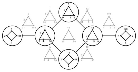
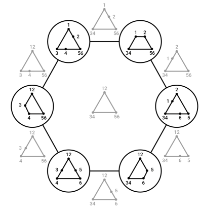
Figure 7: Configurations of type EEFF(a) and type FFFGG in the compactification of $\mathcal{S}(3)$

Figure 7 is a representation of the self-dual matroid subdivisions corresponding to the $105$ triangles in Theorem 6.5, $90$ of type EEFF(a) and $15$ of type FFFGG. The pictures coincide with those in Figure 5, but now we draw configurations for the matroids in each subdivision. The valuated matroid $q$ is self-dual, and $\mathcal{M}(q)$ satisfies the conclusion of Proposition 6.2.

Our discussion is meant to explain the compactification of the self-dual configuration space $\mathcal{S}(3)$ given by Kapranov’s Chow quotient. Figure 7 shows the limit behavior for configurations of six points (like $X\simeq X^{\prime}$) that lie on a conic in $\mathbb{P}^{2}$. It is instructive to compare our pictures to those drawn by Schaffler and Tevelev in [40]. Their diagrams represent the limit behavior of configurations in their Mustafin variety, which is a degeneration of $\mathbb{P}^{2}$. For instance, the picture #20 in [40, Table 15] shows our configuration of type FFFGG.

We conclude with a discussion of the case $n=4$, which is considerably more challenging. Recall from Theorem 2.7 that $\mathcal{S}(4)$ is birational to $\mathcal{R}(4,7)$ via the Cayley octad map $\gamma$. The naive tropicalization of $\gamma$ has undesirable properties, as the following example shows.

Example 6.7.

The naive tropicalization ${\rm trop}(\gamma)$ sends $q\in{\rm Dr}(4,7)$ to the vector $r$ given by

$$r_{I}\,\,=\,\,\begin{cases}q_{I}\quad\quad\quad\quad&\text{ if }8\notin I,\\ q_{I}-\sum_{i\in I}\mu_{i}&\text{ else,}\end{cases}$$

where $\mu_{1},\ldots,\mu_{7}$ are tropicalizations of the Plücker binomials $x_{1},\ldots,x_{7}$ in Theorem 2.7. However, this $r$ fails to lie in the Dressian ${\rm Dr}(4,8)$ for some choices of $q\in{\rm trop}({\rm Gr}(4,7))$.

A choice of $q$ where $r\not\in{\rm Dr}(4,8)$ is the tropical Plücker vector of the $4\times 7$-matrix

$$\small\begin{pmatrix}4t&2t^{5}&-9t^{2}&t^{3}&-5t^{4}&6t^{4}&-9t\\ 9t^{2}&8&3t&4t&3t^{3}&-2t^{4}&5\\ -5t^{4}&3t^{6}&-4t^{2}&3t^{4}&4t^{6}&8t^{4}&t^{2}\\ -3t&-8&6t^{2}&-6t^{4}&-t&-t^{2}&-9t^{3}\end{pmatrix}.$$

Here $r={\rm trop}(\gamma)(q)$ is not a valuated matroid because the ‘min achieved twice’-condition in the Plücker quadric $p_{1234}p_{1358}-p_{1235}p_{1348}+p_{1238}p_{1345}$ is violated. Indeed, we have $r_{1234}=4$, $r_{1358}=18$, $r_{1235}=4$, $r_{1348}=17$, $r_{1238}=15$ and $r_{1345}=5$, so that $\min\{22,21,20\}$ is not achieved twice. This is due to the fact that cancellations appear in the formula for computing $x_{2}$. Classically, we have $\operatorname{val}(x_{2})=\text{val}(-p_{1234}p_{1256}p_{2357}p_{2467}+p_{1235}p_{1246}p_{2347}p_{2567})=21$. But tropically we obtain $\min\{q_{1234}+q_{1256}+q_{2357}+q_{2467},q_{1235}+q_{1246}+q_{2347}+q_{2567}\}=\min\{20,20\}$.

More work is needed to correctly tropicalize the birational isomorphism $\gamma:\mathcal{R}(4,7)\simeq\mathcal{S}(4)$. These are very affine varieties of dimension $9$. The aim would be to parametrize the $9$-dimensional tropical variety ${\rm trop}(\mathcal{S}(4))$ whose points are the tropical Cayley octads. Computing this space is a challenge for the near future. The following serves as point of departure.

Proposition 6.8.

The tropical self-dual Grassmannian ${\rm trop}(\gamma({\rm Gr}(4,7)))={\rm trop}({\rm SGr}(4,8))$ is a balanced fan of pure dimension $16$ in $\mathbb{R}^{70}/\mathbb{R}{\bf 1}$ with $7$-dimensional lineality space. This fan is contained in ${\rm trop}({\rm Gr}(4,8))^{\rm sd}$, which in turn satisfies the following strict inclusion:

$${\rm trop}({\rm Gr}(4,8))^{\rm sd}\,\subsetneq\,{\rm Dr}(4,8)^{\rm sd}.$$ (29)

Proof.

The Fundamental Theorem [26, Theorem 3.2.3] yields the first statement. We have

$${\rm trop}({\rm SGr}(4,8))\,\,\subseteq\,\,{\rm trop}({\rm Gr}(4,8))^{\rm sd}$$ (30)

since the right hand side is the tropical prevariety of the equations that cut out ${\rm SGr}(4,8)$. For the strictness of the inclusion (29), consider the self-dual matroid 4.14.a from Table 1, which is not realizable over $\mathbb{C}$. Starting with this matroid, construct a point $q$ in ${\rm Dr}(4,8)^{\rm sd}$ as follows: $q_{I}=0$ if $I$ is a basis of 4.14.a and $q_{I}=1$ otherwise. The matroid subdivision $\mathcal{M}(q)$ is self-dual. One of its cells is the matroid polytope of 4.14.a. This proves the claim as $q\in\text{trop}({\rm Gr}(4,8))$ would imply that each matroid in $\mathcal{M}(q)$ is realizable over $\mathbb{C}$; see [6]. ∎

Acknowledgments. Many colleagues helped us in this project. We are very grateful for interactions with Daniele Agostini, Tobias Boege, Edgar Costa, Marc Härkönen, Lukas Kühne, Mario Kummer, Marta Panizzut, Yue Ren, Angel David Rios Ortiz, and Benjamin Schröter.

Authors’ addresses:

Alheydis Geiger, MPI-MiS Leipzig alheydis.geiger@mis.mpg.de

Sachi Hashimoto, MPI-MiS Leipzig sachi.hashimoto@mis.mpg.de

Bernd Sturmfels, MPI-MiS Leipzig and UC Berkeley bernd@mis.mpg.de

Raluca Vlad, Brown University raluca_vlad@brown.edu

References

- [1] D. Agostini, C. Fevola, Y. Mandelshtam and B. Sturmfels: KP solitons from tropical limits, Journal of Symbolic Computation 114 (2023) 282-301.
- [2] A. D’Ali, T. Boege, T. Kahle and B. Sturmfels: The geometry of gaussoids, Foundations of Computational Mathematics 19 (2019) 775–812.
- [3] F. Bath: Ten associated points and quartic and quintic curves in [4], Journal of the London Math. Society 13 (1938) 198–201.
- [4] D. Bayer and D. Eisenbud: Graph curves, Advances in Mathematics 86 (1991) 1–40.
- [5] J. Bezanson, A. Edelman, S. Karpinski and V. Shah: Julia: A fresh approach to numerical computing, SIAM Review 59 (2017) 65–98.
- [6] M. Brandt and D. Speyer: Computation of Dressians by dimensional reduction, Advances in Geometry (2022).
- [7] T. Brylawski and D. Lucas: Uniquely representable combinatorial geometries. In Teorie combinatorie (Proc. 1973 Internat. Colloq.), 83–104. Accademia Nazionale dei Lincei, Rome (1976).
- [8] A. Caminata and L. Schaffler: A Pascal’s Theorem for rational normal curves, Bulletin of the London Math. Society 53 (2021) 1470–1485.
- [9] M. Chan: Moduli spaces of curves: classical and tropical, Notices AMS 68 (2021) 1700–1713.
- [10] C. Ciliberto and C. Pedrini: Real abelian varieties and real algebraic curves, Lectures in real geometry (Madrid, 1994), 167–256, Exp. Math., 23, de Gruyter, Berlin, 1996.
- [11] A. Coble: Associated sets of points, Trans. Amer. Math. Soc. 24 (1922) 1–20.
- [12] I. Dolgachev and D. Ortland: Point sets in projective spaces and theta functions, Astérique 165 (1988).
- [13] L. Ein and R. Lazarsfeld: Tangent developable surfaces and the equations defining algebraic curves, Bulletin Amer. Math. Soc. 57 (2020) 23–38.
- [14] D. Eisenbud and S. Popescu: The projective geometry of the Gale transform, J. Algebra 230 (2000) 127–173.
- [15] D. Eisenbud and S. Popescu: Gale duality and free resolutions of ideals of points, Invent. math. 136 (1999) 419–449.
- [16] E. Feichtner and B. Sturmfels: Matroid polytopes, nested sets and Bergman fans, Portugaliae Mathematica 62 (2005) 437–468.
- [17] E. Gawrilow and M. Joswig: polymake: a framework for analyzing convex polytopes, Polytopes—combinatorics and computation (Oberwolfach, 1997), DMV Sem., vol. 29, 43–73, Birkhäuser, Basel, 2000
- [18] A. Geiger, S. Hashimoto, B. Sturmfels and R. Vlad: MathRepo: supplementary material for this article, available at https://mathrepo.mis.mpg.de/selfdual.
- [19] D. Grayson and M. Stillman: Macaulay2, a software system for research in algebraic geometry, available at http://www.math.uiuc.edu/Macaulay2/.
- [20] M. Hoff and G. Staglianò: Explicit constructions of K3 surfaces and unirational Noether-Lefschetz divisors, arXiv:2110.15819.
- [21] M. Kapranov: Chow quotients of Grassmannians, Gel’fand Seminar, 29–110, Adv. Soviet Math., 16, Part 2, Amer. Math. Soc., Providence, RI, 1993.
- [22] M. Kapustka: Relations between equations of Mukai varieties, arXiv:1005.5557v1, 2010.
- [23] M. Kapustka: Projections of Mukai varieties, Mathematica Scandinavica 123 (2018) 191–219.
- [24] S. Keel and J. Tevelev: Geometry of Chow quotients of Grassmannians, Duke Math. J. 134 (2006) 259–311.
- [25] B. Lindström: On binary identically self-dual matroids, European J. Combin. 5 (1984) 55–58.
- [26] D. Maclagan and B. Sturmfels: Introduction to Tropical Geometry, Graduate Studies in Mathematics, vol 161, American Mathematical Society, Providence, 2015.
- [27] M. Michałek and B. Sturmfels: Invitation to Nonlinear Algebra, Graduate Studies in Mathematics, vol 211, American Mathematical Society, Providence, 2021.
- [28] S. Mukai: Curves, K3 surfaces and Fano -folds of genus , Algebraic Geometry and Commutative Algebra in Honor of Masayoshi Nagata (1987) 357–377.
- [29] S. Mukai: Curves and Grassmannians. Algebraic geometry and related topics (Inchon, 1992), 19–40, Conf. Proc. Lecture Notes Algebraic Geom., I, Int. Press, Cambridge, MA, (1993).
- [30] S. Mukai: Curves and symmetric spaces, I, American J. Mathematics 117 (1995) 1627–1644.
- [31] S. Mukai: Curves and symmetric spaces, II, Annals of Mathematics 172 (2010) 1539–1558.
- [32] OSCAR Computer Algebra Research System, https://oscar.computeralgebra.de/.
- [33] J. Oxley: Matroid Theory, Oxford Graduate Texts in Mathematics, vol. 21, edition, 2011.
- [34] L. Pachter and D. Speyer: Reconstructing trees from subtree weights, Appl. Math. Lett. 17 (2004) 615–621.
- [35] C. Padró and I. Gracia: Representing small identically self-dual matroids by self-dual codes, SIAM J. Discrete Math. 20 (2006) 1046–1055.
- [36] A. Paffenholz: polyDB: a database for polytopes and related objects, Algorithmic and experimental methods in algebra, geometry, and number theory, 533–547, Springer, Cham, 2017; https://db.polymake.org/.
- [37] A. Perrot: Identically Self-Dual Matroids, Masters Thesis, Victoria University, Wellington, New Zealand, 2017.
- [38] I. Petrakiev: On self-associated sets of points in small projective spaces, Communications in Algebra 37 (2009) 397–405.
- [39] D. Plaumann, B. Sturmfels and C. Vinzant: Quartic curves and their bitangents, J. Symbolic Computation 46 (2011) 712–733.
- [40] L. Schaffler and J. Tevelev: Compactifications of moduli of points and lines in the projective plane, arXiv:2010.03519.
- [41] B. Sturmfels: Algorithms in Invariant Theory, Texts and Monographs in Symbolic Computation, Springer-Verlag, Vienna, 1993.
- [42] O. Tange: GNU Parallel 2018, March 2018, https://doi.org/10.5281/zenodo.1146014.