Spectroscopic determination of C, N, and O abundances of solar-analog stars based on the lines of hydride molecules

Abstract

Photospheric C, N, and O abundances of 118 solar-analog stars were determined by applying the synthetic-fitting analysis to their spectra in the blue or near-UV region comprising lines of CH, NH, and OH molecules, with an aim of clarifying the behaviors of these abundances in comparison with [Fe/H]. It turned out that, in the range of $-0.6\la$ [Fe/H] $\la+0.3$, [C/Fe] shows a marginally increasing tendency with decreasing [Fe/H] with a slight upturn around [Fe/H] $\sim 0$, [N/Fe] tends to somewhat decrease towards lower [Fe/H], and [O/Fe] systematically increases (and thus [C/O] decreases) with a decrease in [Fe/H]. While these results are qualitatively consistent with previous determinations mostly based on atomic lines, the distribution centers of these [C/Fe], [N/Fe], and [O/Fe] at the near-solar metallicity are slightly negative by several hundredths dex, which is interpreted as due to unusual solar abundances possibly related to the planetary formation of our solar system. However, clear anomalies are not observed in the [C,N,O/Fe] ratios of planet-host stars. Three out of four very Be-deficient stars were found to show anomalous [C/Fe] or [N/Fe] which may be due to mass transfer from the evolved companion, though its relation to Be depletion mechanism is still unclear.

1 Introduction

Carbon (C), nitrogen (N), and oxygen (O) are representatively abundant light elements in the Universe next to hydrogen and helium. They are synthesized or burned inside of a star and expelled at the last stage of stellar evolution out to the galactic gas, but the way how this process undergoes in which kind of stars is different for each element. While O is produced and distributed mainly by short-lived high-mass stars, longer-lived low-to-intermediate mass stars may also contribute to the enrichment of C or N. Therefore, CNO abundances in low-mass main-sequence stars like our Sun can be a clue to studying the chemical evolution of these elements, because such stars have diversified ages and the composition of galactic gas at the time of star formation are retained in their atmospheres. Specifically, the runs of [C/Fe], [N/Fe], and [O/Fe] with a change of [Fe/H] (representative of metallicity) in solar-type stars play an important role in this context.

Given this astrophysical significance, not a few spectroscopic determinations of CNO abundances for solar-type stars have been carried out so far (e.g., Takeda & Honda 2005, and the references therein). However, it does not seem necessarily easy to accomplish a sufficient precision. For example, in the work of Takeda & Honda (2005), C or O abundances derived from permitted and forbidden lines were not in satisfactory agreement. Actually, several disadvantages are involved in using lines of neutral atoms (C i, N i, O i) usually adopted: (i) Usable lines are rather few in number and do not have sufficient strengths. (ii) Many are high-excitation lines and thus considerably dependent upon $T$ (temperature) in late-type stars. (iii) Though forbidden lines ([C i] or [O i]) are inert to $T$, they are so weak and apt to be contaminated by blending. (iv) Stronger lines existing in the near-IR region tend to suffer a considerable non-LTE effect.

In the meantime, another possibility of CNO abundance determinations is to make use of lines of hydride molecules (CH, NH, and OH) in the blue or near-UV region, which however has not been mainstream, because this task comes with several difficulties: (i) These lines are in rather unfavorable wavelength regions (accessibility, line crowdness; etc.). (ii) Since the classical analysis using line-by-line equivalent widths is hardly practicable, it is requisite to compare the observed and theoretically synthesized spectra. (iii) Because of low dissociation potentials, the populations of these molecules are quite sensitive to $T$, which means that resulting abundances are appreciably dependent upon adopted atmospheric models. (iv) More seriously, abundances ($A$) derived from these molecular lines (especially those of UV region such as NH) tend to suffer more or less systematic errors for unknown reasons, as shown by the pioneering work of Laird (1985).

However, although such systematic errors involved in $A$(X) (X = C, N, O) derived from hydride molecules may be unavoidable, differential abundances relative to the Sun ([X/H]; cf. footnote 1) may still be acceptable at least for solar-type stars, because errors tend be cancelled if stars are not much different from the Sun. Actually, several studies revealed that reasonable results of [X/H] could be obtained for FGK-type dwarfs (including planet-host stars) by applying the spectrum-synthesis analysis to molecular line features in the blue–UV region; e.g., Ecuvillon et al. (2006) for OH, Suárez-Andrés et al. (2016) for NH, and Suárez-Andrés et al. (2017) for CH.

If so, it must be more preferable to carry out a differential analysis relative to the Sun exclusively for “solar-analog” stars (Sun-like early G-type dwarfs; cf. footnote 2), by which systematic errors would be largely suppressed. Therefore, sufficient reliability is expected for the differential abundances ([X/H]) of solar analogs; moreover, high precision would be accomplished by averaging the results derived from a number of spectral regions (thanks to the availability of numerous lines for these molecules).

The author’s group previously carried out comprehensive investigations for 118 solar-analog stars in comparison with the Sun, which were published in a series of papers: Takeda et al. (2007) (stellar parameters and Li abundances), Takeda et al. (2010) (stellar activity estimated from Ca ii 8542 and its relation to rotation), Takeda et al. (2011) (behaviors of Be abundances determined from Be ii 3131), and Takeda et al. (2012) (detection of low-level activity using Ca ii 3934). In connection with this project, we acquired high-dispersion spectra of near-UV through blue region ($\sim$ 3000–4600 Å) for all of the sample stars, which were employed for the latter two studies. Since these spectra are just suitable for doing the differential analysis of molecular lines mentioned above, I decided to conduct new CNO abundance determinations of these solar analogs based on CH, NH, and OH lines, while paying attention to the following points.

• How are the behaviors of [C/Fe], [N/Fe], and [O/Fe] with a change of [Fe/H] (e.g., gradient, dispersion, zero-point) within $\pm$ several tenths dex around [Fe/H] $\sim 0$? It is interesting to compare their trends with those previously derived from atomic lines. The variation of [C/O] with [Fe/H] is also an important checkpoint.

• Do stars harboring giant planets show any appreciable difference in terms of CNO abundances in comparison with the sample of non-planet-host stars?

• Takeda et al. (2011) serendipitously found 4 extraordinary Sun-like stars, in which Be is drastically deficient by $\ga 2$ dex compared to the others (and the Sun). It is interesting to check whether these Be-depleted stars exhibit any peculiarities in CNO abundances, which may provide some information on the origin of Be anomaly.

The purpose of this article is to describe the outcome of this analysis.

2 Program stars

2.1 Atmospheric parameters

The sample of 118 solar-analog stars in the solar neighborhood are the same as those adopted in Takeda et al. (2007), which were selected by the criterion of $0.62\la B-V\la 0.67$ and $4.5\la M_{V}\la 5.1$ (centered around the solar values of $(B-V)_{\odot}=0.65$ and $M_{V\odot}=4.82$). Likewise, regarding the atmospheric parameters [$T_{\rm eff}$ (effective temperature), $\log g$ (surface gravity), $v_{\rm t}$ (microturbulence), and [Fe/H] (Fe abundance relative to the solar Fe abundance of $A_{\odot}$(Fe) = 7.50)] of these stars along with the Sun, those spectroscopically determined by Takeda et al. (2007) (standard solutions; cf. sect. 3.1.1 therein) were used unchanged. The list of 118 stars (+ Sun) and their atmospheric parameters are presented in Table 1, where 12 planet-host stars and 4 Be-depleted stars (cf. sect. 4.2 in Takeda et al. 2011) are also indicated. The atmospheric models are the same as adopted in our previous papers (cf. sect. 4.1 of Takeda et al. 2007), which were generated by 3-dimensionally interpolating Kurucz’s (1993a) ATLAS9 grid of model atmospheres in terms of $T_{\rm eff}$, $\log g$, and [Fe/H] (metallicity).

2.2 Errors in $T_{\rm eff}$, $\log g$, and $v_{\rm t}$

As described in sect. 3.1.1 of Takeda et al. (2007), these atmospheric parameters were determined by using the TGVIT program (Takeda et al. 2002, 2005) based on the equivalent widths of Fe i and Fe ii lines, while requiring three conditions to be simultaneously satisfied: (a) independence of $A$(Fe) upon $\chi_{\rm low}$, (b) independence of $A$(Fe) upon the equivalent widths, and (c) matching the mean abundances of $\langle A$(Fe i)$\rangle$ and $\langle A$(Fe ii)$\rangle$. Since solar $gf$ values (cf. sect. 2 in Takeda et al. 2005) were adopted in this application to solar-analog stars, the statistical errors involved in $T_{\rm eff}$, $\log g$, and $v_{\rm t}$ (estimated by the procedure described in sect. 5.2 of Takeda et al. 2002) are sufficiently small, which are typically on the order of $\sim\pm 20$ K, $\sim\pm 0.05$ dex, and $\sim\pm 0.1$ km s^-1, respectively. See also sect. 3.4 in Takeda et al. (2011); the errors derived for individual stars are given in electronic table E3 of that paper.

2.3 Observational data

The high-dispersion spectra of 118 program stars and Vesta (substitute for the Sun) covering $\sim$ 3000–4600 Å with a resolving power of $R\simeq 60000$ used in this study are those obtained in 2009–2010 with the High Dispersion Spectrograph (HDS) placed at the Nasmyth platform of the 8.2-m Subaru Telescope atop Mauna Kea (see sect. 2 of Takeda et al. 2011 for more details).

Table 1: Stellar parameters and the CNO abundance results of 118 program stars.

Star	HIP	$T_{\rm eff}$	$\log g$	$v_{\rm t}$	[Fe/H]	[C/H]	[N/H]	[O/H]	[C/O]	Remark
No.	number	(K)	(dex)	(km s-1)	(dex)	(dex)	(dex)	(dex)	(dex)
1	001499	5724	4.45	0.95	+0.20	+0.20	+0.23	+0.09	+0.12	PHS
2	001598	5693	4.33	0.96	$-$0.27	$-$0.38	$-$0.38	$-$0.24	$-$0.14
3	001803	5817	4.41	1.17	+0.24	+0.11	+0.20	+0.10	+0.01
4	004290	5719	4.40	1.10	$-$0.12	$-$0.21	$-$0.20	$-$0.16	$-$0.04
5	005176	5855	4.39	1.03	+0.19	+0.18	+0.22	+0.14	+0.04
6	006405	5728	4.38	0.96	$-$0.14	$-$0.24	$-$0.28	$-$0.14	$-$0.09
7	006455	5716	4.57	0.99	$-$0.09	$-$0.15	$-$0.18	$-$0.09	$-$0.06
8	007244	5755	4.52	1.12	$-$0.04	$-$0.12	$-$0.12	$-$0.09	$-$0.03
9	007585	5784	4.50	1.04	+0.07	+0.00	$-$0.02	+0.01	+0.00
10	007902	5613	4.39	0.91	$-$0.01	$-$0.05	$-$0.17	$-$0.02	$-$0.03
11	007918	5841	4.30	1.12	+0.01	$-$0.03	+0.00	$-$0.01	$-$0.02
12	008486	5805	4.45	1.13	$-$0.06	$-$0.22	$-$0.23	$-$0.13	$-$0.09
13	009172	5763	4.55	1.12	+0.06	$-$0.08	$-$0.05	$-$0.02	$-$0.06
14	009349	5788	4.35	1.07	+0.01	$-$0.03	+0.01	+0.00	$-$0.03
15	009519	5853	4.45	1.22	+0.14	$-$0.04	$-$0.04	+0.02	$-$0.06	PHS
16	009829	5579	4.25	0.94	$-$0.31	$-$0.36	$-$0.44	$-$0.31	$-$0.06
17	010321	5707	4.60	1.04	+0.00	$-$0.10	$-$0.11	$-$0.09	$-$0.01
18	011728	5708	4.40	1.02	+0.02	$-$0.05	$-$0.03	$-$0.05	+0.00
19	012067	5709	4.41	0.96	+0.20	+0.16	+0.18	+0.09	+0.06
20	014614	5726	4.26	1.00	$-$0.12	$-$0.18	$-$0.19	$-$0.11	$-$0.07
21	014623	5742	4.52	1.09	+0.12	+0.03	+0.08	+0.01	+0.02
22	015062	5735	4.49	0.94	$-$0.29	$-$0.38	$-$0.40	$-$0.23	$-$0.15
23	015442	5682	4.50	0.87	$-$0.19	$-$0.25	$-$0.29	$-$0.16	$-$0.10
24	016405	5738	4.32	1.03	+0.26	+0.27	+0.25	+0.17	+0.10
25	017336	5671	4.55	0.94	$-$0.13	$-$0.21	$-$0.01	$-$0.11	$-$0.10	BED
26	018261	5873	4.43	0.97	+0.02	$-$0.06	$-$0.03	+0.04	$-$0.10
27	019793	5828	4.51	1.26	+0.19	+0.08	+0.15	+0.05	+0.03
28	019911	5672	4.34	1.10	$-$0.13	$-$0.33	$-$0.37	$-$0.32	$-$0.02
29	019925	5767	4.53	0.99	+0.07	+0.01	+0.03	+0.02	$-$0.01
30	020441	5771	4.42	1.10	+0.13	+0.10	+0.17	+0.05	+0.05
31	020719	5831	4.36	1.24	+0.13	+0.02	+0.13	$-$0.02	+0.04
32	020741	5797	4.37	1.20	+0.16	+0.09	+0.17	+0.05	+0.04
33	020752	5923	4.46	1.13	+0.16	+0.03	+0.05	+0.06	$-$0.03
34	021165	5760	4.28	0.99	$-$0.16	$-$0.26	$-$0.31	$-$0.15	$-$0.11
35	021172	5625	4.27	0.90	$-$0.10	$-$0.16	$-$0.27	$-$0.08	$-$0.07
36	022203	5740	4.33	1.07	+0.13	+0.05	+0.12	+0.00	+0.05
37	023530	5601	4.36	0.91	$-$0.24	$-$0.18	$-$0.18	$-$0.11	$-$0.07
38	025002	5729	4.47	1.07	$-$0.08	$-$0.23	$-$0.26	$-$0.21	$-$0.02
39	025414	5635	4.49	0.89	+0.10	+0.09	+0.06	+0.01	+0.08
40	025670	5759	4.55	0.88	+0.10	+0.04	+0.06	+0.08	$-$0.04
41	026381	5518	4.47	0.87	$-$0.45	$-$0.47	$-$0.65	$-$0.31	$-$0.16	PHS
42	027435	5697	4.45	0.93	$-$0.22	$-$0.27	$-$0.28	$-$0.18	$-$0.09	PHS
43	029432	5712	4.32	1.00	$-$0.12	$-$0.14	$-$0.16	$-$0.11	$-$0.03	PHS
44	031965	5770	4.31	0.99	+0.05	+0.02	+0.00	+0.03	$-$0.01
45	032673	5724	4.57	0.95	+0.06	+0.06	+0.23	+0.01	+0.05	BED
46	033932	5891	4.38	1.10	$-$0.12	$-$0.20	$-$0.22	$-$0.07	$-$0.13
47	035185	5793	4.19	1.35	+0.00	$-$0.14	$-$0.08	$-$0.07	$-$0.08
48	035265	5804	4.37	1.04	$-$0.02	$-$0.05	$-$0.04	$-$0.04	$-$0.02
49	036512	5718	4.49	0.89	$-$0.09	$-$0.13	$-$0.17	$-$0.08	$-$0.04
50	038647	5714	4.43	0.95	+0.01	$-$0.14	$-$0.15	$-$0.06	$-$0.07
51	038747	5804	4.42	1.05	+0.06	$-$0.08	$-$0.08	+0.00	$-$0.08
52	038853	5899	4.27	1.03	$-$0.05	$-$0.12	$-$0.14	$-$0.05	$-$0.07
53	039506	5600	4.24	0.83	$-$0.62	$-$0.69	$-$0.92	$-$0.40	$-$0.29
54	039822	5758	4.35	0.90	$-$0.22	$-$0.26	$-$0.32	$-$0.12	$-$0.14
55	040118	5541	4.45	0.84	$-$0.42	$-$0.43	$-$0.63	$-$0.29	$-$0.14
56	040133	5698	4.33	0.97	+0.12	+0.05	+0.05	+0.03	+0.02
57	041184	5705	4.43	1.51	+0.11	$-$0.09	+0.06	$-$0.10	+0.02
58	041484	5864	4.33	0.92	+0.05	+0.02	+0.02	+0.07	$-$0.06
59	041526	5801	4.27	0.98	$-$0.02	$-$0.10	$-$0.14	$-$0.02	$-$0.08
60	042333	5816	4.44	1.08	+0.14	+0.05	+0.10	+0.06	$-$0.01
61	042575	5675	4.40	0.96	+0.06	+0.00	+0.00	+0.00	+0.00
62	043297	5691	4.46	1.05	+0.08	+0.01	+0.02	+0.02	$-$0.01
63	043557	5805	4.42	1.05	$-$0.06	$-$0.06	$-$0.07	$-$0.05	$-$0.01
64	043726	5769	4.47	1.01	+0.11	+0.09	+0.16	+0.03	+0.06
65	044324	5888	4.45	1.09	$-$0.01	$-$0.08	$-$0.11	$-$0.02	$-$0.06

Table 1: (Continued.)

Star	HIP	$T_{\rm eff}$	$\log g$	$v_{\rm t}$	[Fe/H]	[C/H]	[N/H]	[O/H]	[C/O]	Remark
No.	number	(K)	(dex)	(km s-1)	(dex)	(dex)	(dex)	(dex)	(dex)
66	044997	5696	4.54	0.75	+0.04	$-$0.03	+0.01	+0.02	$-$0.05
67	045325	5935	4.47	0.97	+0.18	+0.17	+0.22	+0.22	$-$0.06
68	046903	5746	4.40	1.11	$-$0.03	$-$0.10	$-$0.10	$-$0.06	$-$0.04
69	049580	5782	4.41	0.87	+0.02	$-$0.05	$-$0.05	+0.03	$-$0.08
70	049586	5786	4.42	1.06	+0.20	+0.15	+0.18	+0.12	+0.03
71	049728	5744	4.40	0.98	$-$0.07	$-$0.09	$-$0.12	$-$0.06	$-$0.03
72	049756	5720	4.28	0.99	+0.02	$-$0.02	$-$0.01	$-$0.02	+0.00
73	050505	5590	4.44	0.84	$-$0.17	$-$0.23	$-$0.29	$-$0.19	$-$0.04
74	051178	5801	4.47	0.87	$-$0.17	$-$0.20	$-$0.23	$-$0.12	$-$0.08
75	053721	5819	4.19	1.15	$-$0.02	$-$0.05	$-$0.01	$-$0.03	$-$0.02	PHS
76	054375	5803	4.37	0.96	+0.14	+0.03	+0.06	+0.05	$-$0.02
77	055459	5812	4.36	1.03	+0.07	+0.03	+0.02	+0.05	$-$0.02
78	055868	5757	4.49	0.95	$-$0.15	$-$0.25	$-$0.27	$-$0.12	$-$0.12
79	059589	5654	4.51	0.70	$-$0.01	$-$0.04	$-$0.16	+0.04	$-$0.09
80	059610	5829	4.34	1.04	$-$0.06	$-$0.09	$-$0.09	$-$0.05	$-$0.04	PHS
81	062175	5683	4.19	0.90	+0.13	+0.02	+0.00	+0.01	+0.01
82	062816	5804	4.43	0.97	+0.06	$-$0.04	+0.00	+0.00	$-$0.04
83	063048	5655	4.32	0.91	$-$0.02	$-$0.01	$-$0.11	+0.00	$-$0.02
84	063636	5799	4.52	1.10	$-$0.01	$-$0.05	$-$0.08	$-$0.04	+0.00
85	064150	5726	4.42	0.99	+0.05	+0.05	+0.03	+0.00	+0.05	BED
86	064747	5710	4.42	0.93	$-$0.18	$-$0.20	$-$0.26	$-$0.10	$-$0.09
87	070319	5678	4.42	0.96	$-$0.33	$-$0.35	$-$0.50	$-$0.24	$-$0.11	PHS
88	072604	5655	4.24	0.84	$-$0.14	$-$0.19	$-$0.30	$-$0.07	$-$0.11
89	075676	5772	4.44	0.88	$-$0.08	+0.09	$-$0.05	$-$0.07	+0.17	BED
90	076114	5709	4.42	1.02	$-$0.02	$-$0.05	$-$0.05	$-$0.05	+0.00
91	077749	5836	4.61	1.14	+0.22	+0.08	+0.14	+0.09	$-$0.02
92	078217	5749	4.43	1.10	$-$0.22	$-$0.32	$-$0.33	$-$0.17	$-$0.16
93	079672	5768	4.40	0.96	+0.04	$-$0.03	$-$0.02	+0.00	$-$0.03
94	085042	5676	4.48	0.99	+0.03	$-$0.03	$-$0.06	$-$0.03	+0.01
95	085810	5856	4.46	1.08	+0.15	+0.11	+0.16	+0.10	+0.01
96	088194	5693	4.33	0.98	$-$0.08	$-$0.15	$-$0.18	$-$0.09	$-$0.06	PHS
97	088945	5800	4.38	1.44	$-$0.01	$-$0.19	$-$0.05	$-$0.17	$-$0.02
98	089282	5833	4.22	1.00	+0.00	$-$0.11	$-$0.14	$-$0.05	$-$0.06
99	089474	5755	4.20	1.04	+0.01	$-$0.01	$-$0.01	+0.01	$-$0.02	PHS
100	089912	5846	4.38	1.24	+0.04	$-$0.11	$-$0.08	$-$0.06	$-$0.05
101	090004	5607	4.42	0.85	$-$0.01	$-$0.04	$-$0.17	+0.03	$-$0.07	PHS
102	091287	5648	4.46	0.88	$-$0.01	$-$0.06	$-$0.11	$-$0.06	+0.01
103	096184	5863	4.45	1.00	+0.13	+0.12	+0.13	+0.12	+0.00
104	096395	5816	4.48	1.00	$-$0.10	$-$0.15	$-$0.21	$-$0.09	$-$0.06
105	096402	5661	4.20	1.00	$-$0.03	+0.02	$-$0.08	+0.03	+0.00
106	096901	5742	4.32	1.01	+0.08	+0.07	+0.04	+0.05	+0.02	PHS
107	096948	5725	4.36	1.07	+0.07	+0.04	+0.04	$-$0.01	+0.04
108	097420	5780	4.42	1.04	+0.05	$-$0.07	$-$0.06	+0.01	$-$0.08
109	098921	5810	4.50	1.19	+0.17	+0.07	+0.10	+0.05	+0.02
110	100963	5779	4.46	0.98	+0.00	$-$0.04	$-$0.05	$-$0.03	$-$0.01
111	104075	5881	4.37	1.08	+0.05	$-$0.09	$-$0.07	$-$0.03	$-$0.06
112	109110	5835	4.51	1.11	+0.07	$-$0.05	$-$0.03	+0.00	$-$0.05
113	110205	5708	4.28	1.08	$-$0.23	$-$0.24	$-$0.25	$-$0.18	$-$0.06
114	112504	5741	4.34	1.00	+0.01	$-$0.09	$-$0.10	$-$0.07	$-$0.02
115	113579	5759	4.21	1.44	+0.05	$-$0.09	+0.09	$-$0.05	$-$0.04
116	113989	5506	4.38	0.74	$-$0.46	$-$0.54	$-$0.73	$-$0.38	$-$0.16
117	115715	5684	4.14	1.05	$-$0.19	$-$0.30	$-$0.34	$-$0.22	$-$0.08
118	116613	5869	4.49	1.11	+0.16	+0.05	+0.12	+0.09	$-$0.04
—	Sun	5761	4.43	1.00	$-$0.01	—	—	—	—

Following the sequentially assigned star No. (Column 1) and Hipparcos catalogue number (Column 2), four atmospheric parameters (effective temperature, surface gravity, microturbulence, Fe abundance relative to the solar abundance of $A_{\odot}$(Fe) = 7.50) taken from Takeda et al. (2007; standard solutions) are given in Columns 3–6. The CNO abundance results derived in this study ([C/H], [N/H], [O/H], [C/O]) are presented in Column 7–10. In Column 11, 12 planet-host stars and 4 Be-depleted stars are remarked as “PHS” and “BED”, respectively. The parameters for the Sun are given in the last row.

3 Abundance determination

3.1 Method of analysis

Since the near-UV through blue spectral regions comprising lines of CH, NH, and OH molecules are considerably crowded with lines, abundance determination should be done by comparing the observed and theoretically synthesized spectra with each other. For this purpose, Takeda’s (1995) automatic spectrum-fitting technique was applied by employing the MPFIT program written by Y. Takeda based on Kurucz’s (1993a) WIDTH9 code. This method aims to match the observed (flux) spectrum in an arbitrary scale ($f^{\rm obs}_{\lambda}$) with the theoretical flux $F^{\rm th}_{\lambda}$, which is a function of various parameters; e.g., wavelength shift ($\Delta\lambda$), macrobroadening velocity ($v_{\rm M}$: $e$-folding half-width of the Gaussian macrobroadening function, $f_{\rm M}(v)\propto\exp[(-v/v_{\rm M})^{2}]$), elemental abundances ($A_{1}$, $A_{2}$, $\ldots$), etc. In addition, two temporary parameters for adjusting $f^{\rm obs}_{\lambda}$ are also included: $C$ (scale control; cf. sect. 2 in Takeda 1995) and $\beta$ (tilt control; cf. footnote 3 in Takeda & Tajitsu 2014). The final solutions accomplishing the best match between theory and observation are obtained by numerically searching the multi-parameter space by applying the Newton–Raphson algorithm. Note that this method does not require any necessity of normalizing the observed spectrum by the local continuum in advance, which is a distinct merit because precisely placing the continuum level is very difficult in the present case.

In order to fit the line features of XH molecules (X = C or N or O), a depth-independent scale factor $\phi$(XH) was introduced, by which the number population of XH molecules (computed from a model atmosphere with the metallicity-scaled X abundance $A_{\rm model}$(X)) is to be multiplied to reproduce the observed XH line strengths. Then, the X abundance of a star $A$(X) was assumed to relate with $\phi$(XH) as $A$(X) = $A_{\rm model}$(X) + $\log\phi$(XH). Note that this implicitly assumes that the population of XH is proportional to the composition of X, which is practically valid in the atmospheric condition of solar-analog stars where the number population of XH molecule is only a minor fraction of the total number of X nuclei (i.e., most are in the form of neutral atoms).

3.2 Spectral regions and line data

The spectral regions comprising CH, NH, and OH lines, where the fitting analysis for abundance determination is performed, were selected after exploratory test runs at 4270–4330 Å (CH), 3340–3390 Å (NH), and 3100–3200 Å (OH). The finally adopted regions (12, 11, and 11 for CH, NH, and OH; each being typically $\sim$ 0.5–2 Å wide) are summarized in Table 2. This table also contains the elements whose abundances were varied (along with $\Delta\lambda$ and $v_{\rm M}$) in the iterative analysis, while the abundances of all other elements were fixed at the metallicity-scaled solar abundances.

Regarding the molecular line data of CH, NH, and OH in these regions, the files “ch.asc”, “nh.asc”, and “oh.asc” downloaded from Kurucz’s homepage (http://kurucz.harvard.edu/linelists/linesmol/) were invoked. The $\log gf$ values in these files were further scaled with the standard isotope ratios by using Kurucz’s (1993b) “RMOLEC.FOR” program. Meanwhile, the data of atomic lines were taken from the VALD database (Ryabchikova et al. 2015). In case that damping parameters are not available, the default treatments used in Kurucz’s (1993a) WIDTH9 program were employed. The finally adopted line data are presented as the supplementary electronic data (directory “linedat”; cf. Appendix A).

As to the dissociation potentials ($D_{0}$), the data already incorporated in the WIDTH9 code were adopted for CH (3.465 eV) and OH (4.392 eV) unchanged, which are almost the same as used by Suárez-Andrés et al. (2017) and Ecuvillon et al. (2006), respectively. However, $D_{0}$ for NH was replaced by 3.37 eV (instead of the original 3.47 eV) according to Suárez-Andrés et al. (2016).

Table 2: Adopted regions and varied abundances in the fitting analysis.

No.	Region code	$\lambda_{1}$	$\lambda_{2}$	Varied abundances
(C abundance determination)
1	CH4273	4273.02	4274.36	Fe, CH
2	CH4277	4276.49	4277.94	Fe, CH, Zr
3	CH4280	4279.19	4281.48	Mn, Fe, CH, Cr, Ti, Sm
4	CH4284	4283.90	4285.25	CH, Ni, Cr, Fe, Ti, Mn
5	CH4286	4285.62	4287.21	Ti, Fe, CH
6	CH4295	4295.54	4296.44	Ti, Ni, Cr, CH
7	CH4297	4297.37	4298.42	Fe, CH, Cr
8	CH4309	4309.23	4310.33	Fe, Y, CH
9	CH4312	4312.39	4313.31	Ti, CH, Mn, Fe
10	CH4313	4313.30	4314.60	Sc, Fe, CH
11	CH4323	4322.41	4324.57	CH
12	CH4328	4327.40	4328.81	Fe, CH
(N abundance determination)
1	NH3340	3340.10	3341.04	Ti, Fe, NH
2	NH3357	3356.98	3357.63	Zr, Cr, NH, Fe
3	NH3358	3357.63	3358.38	Ti, NH, Fe
4	NH3362	3362.50	3363.07	Ni, Ti, NH, Cr
5	NH3363	3363.11	3363.86	Cr, Ni, Fe, NH, Zr, Co
6	NH3364	3364.45	3365.35	Ni, NH, Fe, Co
7	NH3365	3365.32	3366.04	Ni, NH, Fe
8	NH3370	3370.09	3371.22	Fe, Ti, Co, NH
9	NH3382	3382.10	3382.84	Cr, Fe, Ti, NH
10	NH3387	3386.95	3387.70	Fe, Ni, Co, NH
11	NH3388	3388.36	3389.07	Ti, Fe, NH
(O abundance determination)
1	OH3103	3102.79	3103.95	Ti, Fe, Cr, OH
2	OH3105	3105.25	3106.43	Ti, Ni, Fe, OH
3	OH3117	3117.51	3118.09	Ti, OH, Fe
4	OH3124	3123.62	3124.60	OH, Ti, Fe
5	OH3126	3125.83	3127.17	V, Fe, Zr, OH
6	OH3141	3141.36	3142.61	Fe, V, OH, Ti
7	OH3147	3146.83	3147.71	Cr, Fe, Co, OH
8	OH3149	3149.57	3150.18	Cr, OH, Fe
9	OH3168	3168.23	3169.27	Ti, Fe, OH, Cr
10	OH3189	3188.69	3189.66	Fe, OH, Ti
11	OH3191	3191.48	3192.14	Fe, Ti, OH, Zr, Ni

In Columns 3 and 4, $\lambda_{1}$ and $\lambda_{2}$ are the starting and ending wavelengths (in Å) of the spectral region where the fitting analysis was done.

3.3 Analysis results

The iterative solution converged successfully in most of the 34 (=12+11+11) regions for the 118 stars as well as the Sun (Vesta), though some parameters (abundances or $v_{\rm M}$) had to be fixed in exceptional cases (especially for broader-line stars of comparatively higher rotational velocity) in order to avoid instability or divergence.

How the theoretical spectrum for the converged parameter solutions match the observed one is illustrated for each of the spectral regions in Figure 1 (CH), Figure 2 (NH), and Figure 3 (OH) for the case of the Sun. (The information regarding which lines of which species contribute to the complex spectral features of these figures may be found from the line data files in the directory “linedat” mentioned in Sect. 3.2; i.e., line-to-continuum opacity ratios $\eta$ computed for all lines are useful.) Similar figures showing the accomplished spectrum fit for all 118 stars and the relevant data of observed/theoretical spectra are presented as the supplementary electronic data (directories “fitfigs” and “specdat”; cf. Appendix A).

The resulting CNO abundances for the Sun [$A_{\odot}$(C), $A_{\odot}$(N), and $A_{\odot}$(O)] derived for each region are displayed together in Figure 4, where the reference solar abundances taken from two compilations (Anders & Grevesse 1989; Asplund et al. 2009) are also shown for comparison. We can see from this figure that CH, NH, and OH lines in the blue or near-UV region tend to yield more or less lower abundances (especially for N and O). as compared to the actual values. This is the tendency already found by Laird (1985) (cf. Sect. 1). The reason for this systematic error is not clear, for which several possibilities may be considered; such as missing opacity, overdissociation, 3D effect, etc. In any event, this problem involving the absolute scale of $A$ is irrelevant in the present case, because we aim to do a purely differential region-by-region analysis relative to the Sun.

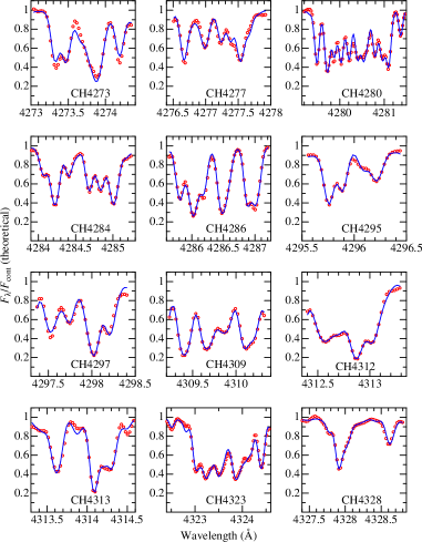
Figure 1: Observed and fitted theoretical spectra in each of the 12 regions (within 4270–4330 Å), where C abundances were determined from CH lines. Shown here is the representative case of the solar (Vesta) spectrum. The observed and theoretical spectra are depicted by red open symbols and blue lines, respectively. The corresponding region code (cf. Table 2) is specified in each panel. The wavelength scale of the spectrum is adjusted to the laboratory frame, and the scale marked in the left ordinate corresponds to the theoretical residual flux ($F^{\rm th}_{\lambda}/F^{\rm th}_{\rm cont}$).

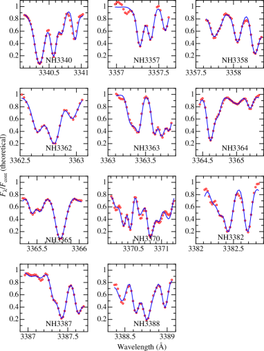
Figure 2: Observed and fitted theoretical solar spectra in each of the 11 regions (within 3340–3390 Å), where N abundances were determined from NH lines. Otherwise, the same as in Figure 1.

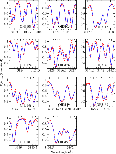
Figure 3: Observed and fitted theoretical solar spectra in each of the 11 regions (within 3100–3200 Å), where O abundances were determined from OH lines. Otherwise, the same as in Figure 1.

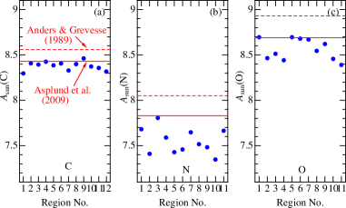
Figure 4: The results of C, N, and O abundances for the Sun ($A_{\odot}$; logarithmic number abundance in the usual normalization of $A_{\rm H}=12$), which were derived from the fitting analysis of solar (Vesta) spectrum in each region, are plotted against the corresponding region number. The left, middle, and right panels are for C, N, and O, respectively. The reference solar CNO abundances published by Anders & Grevesse (1989) (8.56, 8.05, 8.93) and Asplund et al. (2009) (8.43, 7.83, 8.69) are indicated by the horizontal dashed and solid lines, respectively.

3.4 Mean abundances and their errors

Let the abundance of X (= C or N or O) derived from region $i$ be $A_{*i}$ (star) or $A_{\odot i}$ (Sun). Then, the mean differential abundance relative to the Sun averaged over the available regions is defined as

$$\langle[{\rm X/H}]\rangle\equiv\sum_{i=1}^{n_{\rm s}}{([{\rm X/H}]_{i})}/n_{\rm s}\equiv\sum_{i=1}^{n_{\rm s}}{(A_{*i}-A_{\odot i})}/n_{\rm s}\;,$$ (1)

where $n_{\rm s}$ is the number of selected regions finally used for averaging. Since the standard deviation around this mean is

$$\sigma\equiv\sqrt{\sum_{i=1}^{n_{\rm s}}{([{\rm X/H}]_{i}-\langle[{\rm X/H}]\rangle)^{2}}/n_{\rm s}}\;,$$ (2)

the mean error involved in $\langle[{\rm X/H}]\rangle$ is written as

$$\epsilon\equiv\sigma/\sqrt{n_{\rm s}}\;.$$ (3)

Figure 5 (upper 9 panels) shows the dispersion of each $[{\rm X/H}]_{i}$ around $\langle[{\rm X/H}]\rangle$ and the extent of mean error ($\pm\epsilon$) for all 118 stars, while the distribution histograms of $\epsilon$ are illustrated in the bottom 3 panels. As seen from these histograms, most $\epsilon$ values are within $\la$ 0.01–0.02 dex, although several stars (mostly those of broader lines) exceptionally show larger $\epsilon$ amounting up to $\sim$ 0.03–0.04 dex. Actually, mean $\epsilon$ values averaged all stars are ($\langle\epsilon_{\rm C}\rangle$, $\langle\epsilon_{\rm N}\rangle$, $\langle\epsilon_{\rm O}\rangle$) = (0.007, 0.011, 0.011) dex. The detailed results of each region’s [X/H]_i, $\langle[{\rm X/H}]\rangle$, $\sigma$, and $\epsilon$ (X = C, N, O) for all the program stars are summarized in the files “relabs_ch.dat”, “relabs_nh.dat”, and “relabs_oh.dat” (placed in the directory “abunds”) of the supplementary material (cf. Appendix A).

Another error source we have to take into consideration is ambiguities in the atmospheric parameters. As mentioned in Sect. 2.2, the typical statistical errors involved in $T_{\rm eff}$, $\log g$, and $v_{\rm t}$ are $\sim\pm 20$ K, $\sim\pm 0.05$ dex, and $\sim\pm 0.1$ km s^-1,respectively. In order to estimate the impact of these errors, the fitting analysis for the solar spectrum was repeated by perturbing these parameters interchangeably to see the resulting abundance changes ($\delta_{T\pm}$, $\delta_{g\pm}$, $\delta_{v\pm}$) and their root-mean-square ($\delta_{Tgv}$). The results are depicted in Figure 6, which indicates that $\delta_{Tgv}$ is essentially determined by $\delta_{T\pm}$ (reflecting the large $T$-sensitivity) and $\delta_{Tgv}$ is typically $\sim$ 0.02–0.03 dex. As this $\delta_{Tgv}$ acts rather similarly to each [X/H]_i (i.e., not random but in the same direction), $\langle[{\rm X/H}]\rangle$ suffers also this amount of ambiguities due to parameter uncertainties (maily determined by that of $T$).

Accordingly, combining these two kinds of errors ($\epsilon$ and $\delta_{Tgv}$), the typical extent of total error involved in $\langle[{\rm X/H}]\rangle$ would finally make $\la 0.03$ dex.

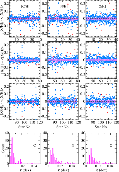
Figure 5: In the upper 9 panels, differences between each [X/H] (X is C/N/O in the left/middle/right panels) of region $i$ ([X/H]_i) and the mean [X/H] over the regions ($\langle$[X/H]$\rangle$) are plotted (in blue symbols) for each of the 118 program stars, which helps to understand the extent of dispersion around the mean. The outlier values (judged by Chauvenet’s criterion) excluded from the averaging process are indicated by red crosses. The pink error bars show the size of mean error ($\pm\epsilon$) of $\langle$[X/H]$\rangle$. In the lowest three panels are shown the distribution histograms for $\epsilon$.

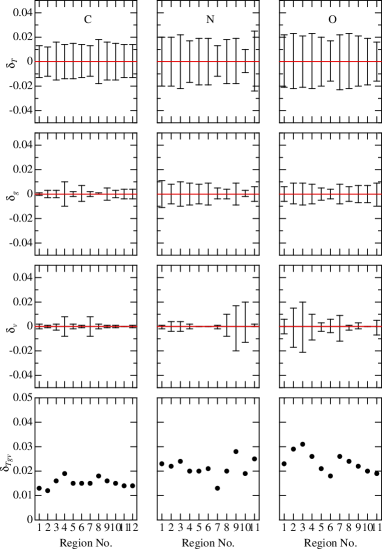
Figure 6: Effect on changing atmospheric parameters on the [X/H] result of each region calculated for the representative case of the Sun, where left, middle, and right panels are for C, N, and O, respectively. 1st-row panels: $\delta_{T+}$ and $\delta_{T-}$ (abundance variations in response to $T_{\rm eff}$ changes by $\pm 20$ K). 2nd-row panels: $\delta_{g+}$ and $\delta_{g-}$ (abundance variations in response to $\log g$ changes by $\pm 0.05$ dex). 3rd-row panels: $\delta_{v+}$ and $\delta_{v-}$ (abundance variations in response to perturbing the $v_{\rm t}$ value by $\pm 0.1$ km s^-1). 4th-row panels: root-sum-square of these three kinds of $\delta$’s, which is defined as $\delta_{Tgv}\equiv(\delta_{T}^{2}+\delta_{g}^{2}+\delta_{v}^{2})^{1/2}$, where $\delta_{T}\equiv(|\delta_{T+}|+|\delta_{T-}|)/2$, $\delta_{g}\equiv(|\delta_{g+}|+|\delta_{g-}|)/2$, and $\delta_{v}\equiv(|\delta_{v+}|+|\delta_{v-}|)/2$.

4 Discussion

4.1 CNO-to-Fe abundance ratios

Now that the relative abundances [X/H] (X = C, N, O) have been established, we can examine the trends of [X/Fe] ($\equiv$ [X/H]$-$[Fe/H]; logarithmic X-to-Fe abundance ratio). derived for solar-analog stars from hydride molecules in comparison with previous results, especially with those of Takeda & Honda (2005) determined for solar-type stars in a broader sense (FGK dwarfs/subgiants) by using atomic lines. How the resulting [X/H] and [X/Fe] are correlated with [Fe/H] (and also the mutual correlation between C and O) is displayed in the left and middle panels of Figure 7. The mean values averaged over each 0.1 dex bin of [Fe/H] between $-0.3\leq$ [Fe/H] $\leq+0.3$ are illustrated in the right panels of this figure, where the corresponding Takeda & Honda’s (2005) results for FGK stars (derived from C i 5052/5380, N i 8680, and O i 7771–5 lines shown in their fig. 6) are also plotted for comparison.

We can see that [C/H] almost scales with [Fe/H] (Fig. 7a), while a systematic departure begins to appear for [N/H] ($<$ [Fe/H]; Fig. 7b) and [O/H] ($>$ [Fe/H]; Fig. 7c) with a decrease in [Fe/H]. As a result, although [C/Fe] does not show so clear [Fe/H]-dependence (Fig. 7e), [N/Fe] tends to decrease (Fig. 7f) while [O/Fe] increases (Fig. 7g) with a lowering of [Fe/H]. Accordingly, [C/O] (= [C/Fe]$-$[O/Fe]) exhibits a progressive decrease towards lower metallicity. (Fig. 7f). The linear-regression relations determined by the least-squares fit are [C/Fe] = $-0.046(\pm 0.032)$[Fe/H] $-0.067(\pm 0.005)$, [N/Fe] = $+0.242(\pm 0.037)$[Fe/H] $-0.068(\pm 0.006)$, [O/Fe] = $-0.350(\pm 0.027)$[Fe/H] $-0.035(\pm 0.004)$, and [C/O] = $+0.305(\pm 0.025)$[Fe/H] $-0.031(\pm 0.004)$, as depicted also in the relevant figure panels.

The slopes (d[X/Fe]/d[Fe/H]) of these relations are important in connection with the galactic chemical evolution. Yet, care should be taken in comparing them with other work, because the resulting gradient may depend upon how the sample stars are chosen. Particularly, since our solar-analog stars cover only a comparatively narrow metallicity range (most stars are within $-0.3\la$ [Fe/H] $\la+0.3$), they are rather disadvantageous in this respect. Keeping this in mind, we may state that these trends are more or less in accord (at least qualitatively) with those published in previous studies; e.g., Takeda & Honda (2005) for C and O (note that their results for N suffer large uncertainties and thus unreliable), Ecuvillon et al. (2006) for O, Suárez-Andrés et al. (2016) for N, Suárez-Andrés et al. (2017) for C, Delgado Mena et al. (2021) for C/O, and the references therein.

Yet, some differences are noticeable from a quantitative point of view. Especially, the resulting d[C/Fe]/d[Fe/H] slope of $-0.05$ is apparently shallower than the previous values (e.g., $\sim-0.2$ concluded by Takeda & Honda 2005); but this is due to the fact that (i) The [Fe/H]-dependence of [C/Fe] not linear but shows an appreciable upturn around [Fe/H]$\sim 0$ and (ii) the [Fe/H] range of our sample stars is narrow ($\pm$ several tenths dex around the solar metallicity). For this reason, the gradient for [C/Fe] (and [C/O]) derived here should not be seriously taken.

Meanwhile, attention should be paid also to the intercept values of these regression relations at [Fe/H] $=0$ ($-0.067$, $-0.068$, and $-0.035$ dex for C, N, and O). That is, the gravity center in the distributions of [C/Fe], [N/Fe], and [O/Fe] ratios around [Fe/H] $\sim 0$ is not zero but slightly negative by several hundredths dex, which can also be recognized by eye-inspection of Figure 7e, 7f, and 7g (or from Fig. 7i, 7j, and 7k; blue bullet symbols). Since such a shift was not found in Takeda & Honda’s (2005) results for FGK stars (cf. pink bullets in Fig. 7i, 7j, and 7k), this detection is a consequence of high-precision relative abundances, which could be accomplished thanks to the effective differential analysis between the Sun and solar-analog stars. This zero-point offset in [C/Fe], [N/Fe], and [O/Fe] is a significant feature in relation to the status of our Sun among the solar-analog stars, as mentioned in the next Section 4.2.

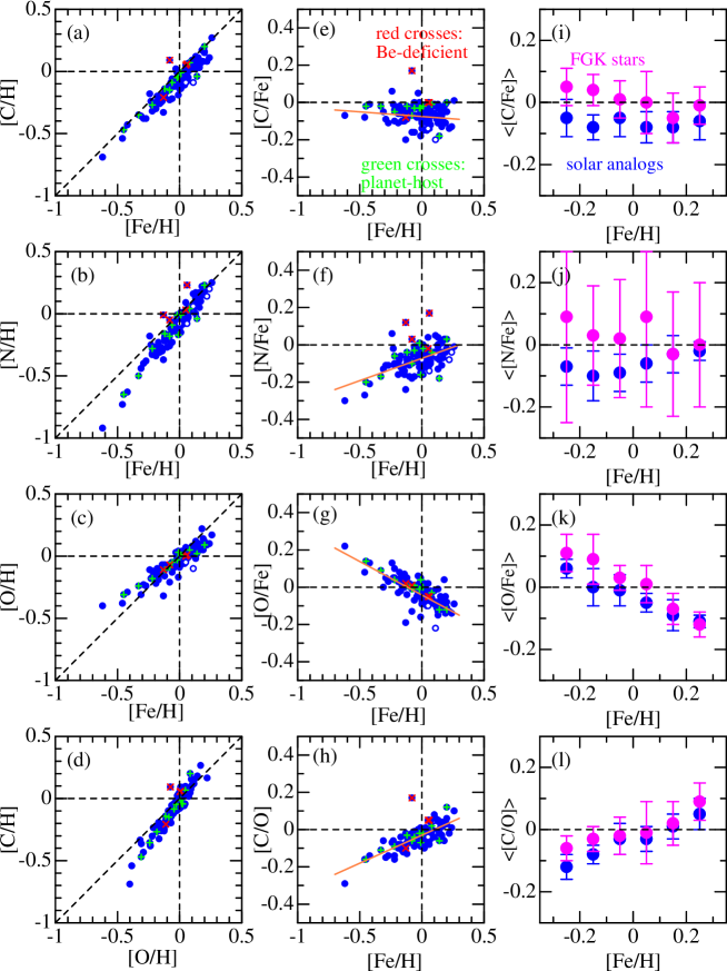
Figure 7: In the left- and middle-column panels are shown the correlations between [X/H] (logarithmic abundance of element X relative to the Sun; X = C or N or O or Fe) and their differences (e.g., [C/Fe] $\equiv$ [C/H] $-$ [Fe/H]): (a) [C/H] vs. [Fe/H], (b) [N/H] vs. [Fe/H], (c) [O/H] vs. [Fe/H], (d) [C/H] vs. [O/H]. (e) [C/Fe] vs. [Fe/H], (f) [N/Fe] vs. [Fe/H], (g) [O/Fe] vs. [Fe/H], and (h) [C/O] vs. [Fe/H]. Less reliable values ($\epsilon>0.03$ dex) are indicated by open symbols; and green crosses (+) and red crosses ($\times$) are overplotted for 12 planet-host stars and 4 Be-deficient stars, respectively. In panels (e)–(h), the linear-regression lines determined by the least-squares analysis are also drawn by the orange solid lines. The bullet symbols in the right-column panels are the mean $\langle$[X/Y]$\rangle$ at each metallicity group (0.1 dex bin within $-0.3\leq$ [Fe/H] $\leq+0.3$) determined for 118 solar analogs (blue, this study) and 160 FGK dwarfs (pink, Takeda & Honda 2005; the results shown in their fig. 6) for comparison, where error bars denote the standard deviations ($\sigma$). Panels (i), (j), (k), and (l) are for $\langle$[C/Fe]$\rangle$, $\langle$[O/Fe]$\rangle$, $\langle$[N/Fe]$\rangle$, and $\langle$[C/O]$\rangle$, respectively.

4.2 Star–planet connection

In order to examine whether stars harboring giant planets show any difference in their CNO abundances, 12 planet-host stars included in our 118 program stars are discriminated by overplotting green crosses in Figure 7a–7h. These figures do not reveal distinct differences between planet-host stars and no-planet samples (i.e., most of the green crosses distribute near to the red linear-regression line showing the mean trend). Yet, some systematic tendency of [X/Fe](with planets) being slightly higher than [X/Fe](without planets) might be seen (especially for [C/Fe] in Fig. 7e). In order to check this point quantitatively, the difference ($d$) between [X/Fe] for each planet-harboring star and $\langle$[X/Fe]$\rangle$ (mean value in the relevant metallicity bin) was calculated and compared with $\sigma$ (standard deviation of the distribution at the coresponding bin), as done by Takeda & Honda (2005) (cf. sect. 5.2 and table 3 in their paper). It then turned out that, while $\sim$70% of the $d$ values of these stars are positive (i.e., relatively overabundant trend on the average), the deviations ($d$) do not exceed $1.5\sigma$ in most cases ($d\sim 1.7$ at the largest). This makes us feel that it is still premature to consider this trend as real. Further studies on a much larger sample of planet-host stars would be required to confirm or disconfirm the reality of this suspected tendency. Accordingly, a conservative statement is retained for the time being that the photospheric CNO abundances of solar-analog stars are not significantly affected by whether they host giant planets or not. This conclusion is almost consistent with the consequences of Suárez-Andrés et al. (2016) for N, and Suárez-Andrés et al. (2017) for C. However, it does not lend support to Ecuvillon et al.’s (2006) argument for O that planet-host stars appear to show an oxygen overabundance by $\sim$ 0.1–0.2 dex in comparison with the reference sample.

As a topic relevant to the influence of planet formation upon photospheric abundances of a host star, the issue of zero-point offset in the [X/Fe] distribution at [Fe/H] $\sim 0$ (cf. Sect. 4.1) has to be mentioned again. In order to ascertain the results described there, the [X/Fe] values in the near-solar metallicity range of $-0.1\leq$ [Fe/H] $\leq+0.1$ (comprising 62 stars) were averaged, and the mean values ($\langle$[X/Fe]$\rangle$) along with their mean errors ($\pm\epsilon$) turned out $\langle$[C/Fe]$\rangle=-0.063(\pm 0.007)$, $\langle$[N/Fe]$\rangle=-0.070(\pm 0.008)$, and $\langle$[O/Fe]$\rangle=-0.033(\pm 0.005)$, which are in agreement with the [Fe/H] = 0 intercepts resulting from the linear-regression analysis in Section 4.1. Therefore, it is certain that these mean $\langle$[X/Fe]$\rangle$ values are slightly negative (by $\simeq$ 0.06–0.07 dex for C and N, $\simeq$ 0.03 dex for O) at [Fe/H] $\sim 0$.

As a matter of fact, this is closely related to the finding of Meléndez et al. (2009), who reported based on the high-precision differential analysis of 11 solar twins relative to the Sun that the Sun shows a characteristic chemical signature in comparison with the reference sample of solar twins that the refractory elements (such as Fe) are comparatively deficient relative to the volatile ones (such as CNO) by $\sim 20$%, which may be associated with the formation mechanism of our solar system (especially rocky terrestrial planets). As seen from their figure 2, when compared at the same solar metallicity, the volatile elements (CNO) in the Sun are comparatively overabundant than the average of solar twins by $\simeq$ 0.05 dex (C), $\simeq$ 0.06 dex (N), and $\simeq$ 0.03 dex (O), which implies that the mean $\langle$[X/Fe]$\rangle$ of the reference stars at [Fe/H] $\sim 0$ would turn out negative by these amounts. These offset values are satisfactorily consistent with our results. Accordingly, our analysis of 118 solar analogs based on the lines of CH, NH, and OH yielded essentially the same conclusion as they obtained from 11 solar twins (although the lines used for abundance determination are not explicitly described in their paper, C i, N i, and O i lines are likely to have been invoked as seen from the wavelength range of their spectra).

4.3 CNO abundances of Be-dearth stars

Takeda et al. (2011) reported that 4 stars out of 118 solar analogs (program stars of this study) are strikingly Be-depleted (by $\ga 2$ dex). Actually, the lines of Be (and Li) are too weak and undetectable in these extraordinary stars (HIP 17336, 32673, 64150, and 75676). Soon after, Viallet & Baraffe (2012) investigated the impacts of rapid rotation and/or episodic accretion in the pre-main sequence phase (both may induce a global mixing, by which Li and Be are brought to the hot interior and burned out at temperatures of more than several million K) as a possible cause for such an extreme Be depletion.

From a different point of view, Desidera et al. (2016) pointed out that all these 4 peculiar solar analogs are binaries, and at least two of them (HIP 64150 and 75676) have white dwarf companions. This means that they may have suffered accretion of the nuclear-processed (Be-depleted) material from the evolved companion due to mass transfer events in the phase of red giant or asymptotic giant branch, which might be responsible for the Be anomaly. This thought lead Desidera et al. (2016) to study the chemical abundances of C and s-process elements for these 4 stars in order to search for any signature of mass accretion from the companion. Interestingly, they found that HIP 75676 is an apparent barium star showing overabundances of s-process elements (Y, Zr, Ba, La) and C. Therefore, in order to supplement their investigation, it is worthwhile to check the CNO abundances we have determined for these Be-depleted stars (which are marked by red crosses in Fig. 7a–7h). The following consequences can be drawn.

• The [C/Fe] values derived by Desidera et al. (2016) from the CH band at 4300 Å ($-0.12$, $-0.05$, $0.00$, and $+0.21$ for HIP 17336, 32673, 64150, and 75676, respectively) are in reasonable agreement with our results ($-0.08$, $0.00$, $0.00$, and $+0.17$).

• Appreciable anomalies deviating from the mean trend are seen in three cases for C and N (Fig. 7e and 7f): HIP 75675’s [C/Fe] ($=+0.17$), HIP 17336’s [N/Fe] ($=+0.12$), and HIP 32673’s [N/Fe] ($=+0.17$). In contrast, no peculiarity is seen in [O/Fe] for all 4 stars (Fig. 7g). To sum up, three Be-depleted solar analogs (HIP 17336, 32673, and 75676) show some kind of anomaly in either C or N, while HIP 64150 is quite normal in terms of CNO abundances.

• As such, no conclusive evidence could be found for the tentative theory that considerable Be-depletion is caused by contamination of nuclear-processed materials from the companion. Although such an interaction event may have actually occurred in the past (especially for the barium star HIP 75676), the existence of Be-deficient CNO-normal star (HIP 64150) indicates that the solution to this problem is not so simple. Besides, as Desidera et al. (2016) pointed out, even if such an efficient mass transfer takes place in the binary system, it is quantitatively difficult to produce such a drastic Be depletion.

• Accordingly, the question for the mechanism of depleting Be is still open. The role of mass transfer from the companion might have an indirect effect on the deficiency of Be (e.g., induced thermohaline mixing or enhanced internal mixing triggered by episodic accretion), as discussed by Desidera et al. (2016). Also, we should pay attention also to the possibility of Be-depletion caused by an effective mixing (e.g., due to rapid rotation) in the pre main-sequence phase, as discussed by Viallet & Baraffe (2012).

5 Summary and conclusion

Clarifying the behaviors of C, N, and O abundances (representative light elements processed in the stellar core to be dredged up and ejected outwards in the course of stellar evolution) in solar-type low-mass stars of diversified ages is important for studying the chemical evolution history of the Galaxy.

However, precisely establishing the key quantities [C/Fe], [N/Fe], and [O/Fe] (in comparison with the metallicity [Fe/H]) is not necessarily easy, because often adopted atomic C i, N i, and O i lines are small in number and generally weak. A possibility to ameliorate this situation is to invoke the lines of hydride molecules (CH, NH, and OH) numerously available with sufficiently large strengths in blue or near-UV wavelength regions. Although absolute abundances derived from these molecular lines are apt to suffer systematic errors, this problem can be circumvented by carrying out differential analysis relative to the Sun while limiting the sample only to solar-analog stars (early G-type dwarfs).

This consideration motivated the author to determine the C, N, and O abundances of 118 solar-analog stars, whose atmospheric parameters ($T_{\rm eff}$, $\log g$, $v_{\rm t}$, and [Fe/H]) are already established by Takeda et al. (2007), based on the lines of hydride molecules in blue or near-UV regions. For this purpose, extensive spectrum-synthesis analyses based on the efficient automatic fitting algorithm were applied to 12 spectral regions of CH lines (selected from 4270–4330 Å), 11 regions of NH lines (from 3340–3390 Å), and 11 regions of OH lines (from 3100–3200 Å).

The primary aims of this study were (i) to clarify the behaviors of [C/Fe], [N/Fe], and [O/Fe], (ii) to examine whether any abundance characteristics related to the existence of planets is seen, and (iii) to check whether any anomaly exists in the CNO abundances of 4 drastically Be-depleted stars found by Takeda et al. (2011).

The trends of [C/Fe], [N/Fe], and [O/Fe] in relation to [Fe/H] turned out almost consistent (at least qualitatively) with those reported by past studies mainly based on atomic lines: In the metallicity range of $-0.6\la$ [Fe/H] $\la+0.3$, [C/Fe] shows a marginally increasing tendency for decrease of [Fe/H] with a slight upturn around [Fe/H] $\sim 0$, [N/Fe] tends to somewhat decrease towards lower [Fe/H], and [O/Fe] systematically increases (and thus [C/O] decreases) with decreasing [Fe/H].

It is noteworthy, however, that the gravity centers of these [X/Fe] ratios (X = C, N, O) are slightly subsolar (negative) by several hundredths dex ($\simeq$ 0.06–0.07 dex for C and N, $\simeq$ 0.03 dex for O) around [Fe/H] $\sim 0$, which may be interpreted as unusual CNO-to-Fe abundance ratios of the Sun (compared to the mean of other solar analogs). This is essentially a reconfirmation of the finding of Meléndez et al. (2009), who reported that refractory elements (such as Fe) are somewhat deficient relative to the volatile ones (such as CNO) in the solar photosphere in comparison with the sample of 11 solar twins, which they suspected may be related to the formation mechanism of our solar system (especially rocky terrestrial planets).

In the meanwhile, regarding the question whether CNO abundances suffer any influence by the existence of giant planets, clear differences are not seen in the distributions of [C/Fe], [N/Fe], and [O/Fe] for 12 planet-host stars in comparison to other no-planet samples, though a possibility of the former tending to be slightly larger than the latter can not be ruled out.

Given that Desidera et al. (2016) reported that all 4 Be-depleted stars (HIP 17336, 32673, 64150, and 75676) detected by Takeda et al. (2011) are binary systems (especially at least 2 stars have white dwarf companions), it is worthwhile to examine whether they have any CNO anomalies caused by contamination of nuclear-processed materials. Our results indicate that three of them (HIP 17336, 32673, and 75676) show overabundances in either C or N, whereas HIP 64150 is quite normal in terms of CNO abundances. As such, mass transfer from the companion may have actually occurred in these stars (especially, highly probable for the barium star HD 75676). However, it is premature to relate this to the cause of Be anomaly, because this mechanism alone is quantitatively difficult to produce such a drastic Be depletion (by $\ga 2$ dex). Accordingly, the question for the mechanism of depleting Be is still open. Several other interpretations such as those related to pre-main sequence evolution (Viallet & Baraffe 2012) or indirect effect of mass transfer from the companion (Desidera et al. 2016) are worth further investigation.

Appendix A Electronic data tables and figures

Supplementary electronic materials (data tables and figure files) are accompanied with this article, which are separately contained in four directories as described below.

A.1 Atomic and molecular line data

The directory “linedat” contains 34 files named as “lines_??????.dat” (“??????” is the 6-character region code; e.g., CH4273), which include the data of atomic and molecular lines (typically several hundred lines) used for the fitting analysis at each region. The data are basically arranged in the ascending order of wavelength, though atomic and molecular lines are separately grouped in each file, Table A.1 describes the contents of these line data.

A.2 Data of observed and theoretical spectra

In the directory “specdat” are contained 34 files named as “fit_??????.dat” (“??????” is the 6-character region code; e.g., CH4273), which include the observed and fitted theoretical spectra at each region. Each file consists of 119 sections corresponding to 118 program stars and the Sun/Vesta (its number is tentatively designated as 999999). In each section, the first header line includes the information of 6-character HIP number (HIP), number of points ($n_{\rm p}$), first wavelength ($w_{1}$) and last wavelength ($w_{2}$), which can be read with the format (2X,A6,I4,2F10.4). Then, $\lambda$ (wavelength in Å), $f_{\lambda}^{\rm obs}$ (observed spectra) $F_{\lambda}^{\rm the}$ (fitted theoretical spectra) are given with the format (F8.3,2F10.4) in each of the following $n_{\rm p}$ lines. Note that these spectra are the residual flux reduced to the theoretical continuum level ($F_{\rm cont}^{\rm the}$).

A.3 Figures of spectrum fitting

The directory “fitfigs” contains 34 PDF files named as “??????.pdf” (“??????” is the 6-character region code; e.g., CH4273), which include the figures showing the accomplished fit between the observed (red open symbols) and theoretical (blue lines) spectra for each of the 118(+1) stars, which were constructed based on the “fit_??????.dat” files. Each spectrum (indicated by the corresponding HIP number) is vertically shifted by 0.5 relative to the adjacent ones. Note that these figures are arranged in almost the same manner as adopted in our previous papers (e.g., fig. 8 in Takeda et al. 2007 or fig. 4 in Takeda et al. 2011).

A.4 Abundance results derived for each region

Three data files “relabs_ch.dat”, “relabs_nh.dat”, and “relabs_oh.dat” are found in the directory “abunds”, which present the detailed results of relative abundances ([C/H] or [N/H] or [O/H] derived from each of the 11–12 spectral regions) and their means (along with the associated standard deviations and mean errors). Stellar parameters are also included for convenience. After the first header line, the results for each of the 118 stars are given in the 2nd through 119th lines. And the last 120th line is for the Sun/Vesta, where the absolute abundances [$A$(C) or $A$(N) or $A$(O)] resulting from each region (used as the reference abundances) are presented. The data contents and their format are described in Table A.2.

Table 3: Contents of line data files (“lines_??????.dat”).

Bytes	Format	Units	Item	Brief Explanations
1– 9	F9.3	Å	$\lambda$	(air) wavelength
11–16	F6.2	—	s-code	species code(a)
18–20	A3	—	species	notation of species(b)
21–32	E12.4	—	$\eta$	line-strength indicator(c)
33–43	F11.5	—	$\eta$	line-strength indicator(c)
44–51	F8.3	eV	$\chi_{\rm low}$	lower excitation potential
52–59	F8.3	dex	$\log gf$	log of stat. weight (lower level) times osc. strength
60–67	F8.3	dex	Gammar	radiation damping parameter(d)
68–75	F8.3	dex	Gammas	Stark effect damping parameter(d)
76–83	F8.3	dex	Gammaw	van der Waals effect damping parameter(d)

Notes:
^(a)Constructed from the atomic number and ionization stage. For example: O i line $\rightarrow$ 8.00, Fe i line $\rightarrow$ 26.00, Y ii line $\rightarrow$ 39.01, CH line $\rightarrow$ 106.00, NH line $\rightarrow$ 107.00, OH line $\rightarrow$ 108.00.
^(b)For example, Fe1 $\rightarrow$ Fe i, Y2 $\rightarrow$ Y ii.
^(c)Line-center-to-continuum opacity ratio calculated for the solar model atmosphere (with the solar abundances) at $\tau_{5000}=0.2$
^(d)Gammar: logarithm of radiation damping width (s^-1) [$\log\gamma_{\rm rad}$]. Gammas: logarithm of Stark damping width (s^-1) per electron density (cm^-3) at 10000 K [$\log(\gamma_{\rm e}/N_{\rm e})$]. Gammaw: logarithm of van der Waals damping width (s^-1) per hydrogen density (cm^-3) at 10000 K [$\log(\gamma_{\rm w}/N_{\rm H})$].

Table 4: Contents of abundance data files (“relabs_?h.dat”).

Bytes	Format	Units	Item	Brief Explanations
1– 6	I6	—	HIP	Hipparcos catalogue number (999999 is for Sun/Vesta)
7–13	F7.0	K	$T_{\rm eff}$	Effective temperature(a)
14–19	F6.2	dex	$\log g$	Logarithm of surface gravity (in c.g.s.)(a)
20–25	F6.2	km s-1	$v_{\rm t}$	Microturbulent velocity dispersion(a)
26–32	F7.2	dex	[Fe/H]	Differential logarithmic Fe abundance relative to the Sun(a)
33–36	I4	—	$n_{\rm t}$	Total number of spectral regions
37–39	I3	—	$n_{\rm s}$	Number of regions adopted for calculation of mean $\langle$[X/H]$\rangle$
40–46	F7.3	dex	$\langle$[X/H]$\rangle$	Mean of [X/H](b) averaged over different spectral regions
47–52	F6.3	dex	$\sigma$	Standard deviation of $\langle$[X/H]$\rangle$
53–58	F6.3	dex	$\epsilon$	mean error of $\langle$[X/H]$\rangle$ ($\equiv\sigma/\sqrt{n_{\rm s}}$)
60–66	F7.3	dex	[X/H]1	[X/H] value derived in region 1
67–67	A1	—	flag1	Adopt-or-reject flag(c) for [X/H]1
$S_{i}$–$E_{i}$	F7.3	dex	[X/H]i	[X/H] value derived in region $i$ (d)
$F_{i}$–$F_{i}$	A1	—	flagi	Adopt-or-reject flag(c) for [X/H]i(d)

Notes:
^(a)These are the “standard solutions” derived in Takeda et al. (2007) (cf. sect. 3.1.1 therein).
^(b)[X/H] is the differential abundance of X (X is C or N or O) relative to the solar abundance; i.e., [X/H] $\equiv$ $A_{*}({\rm X})-A_{\odot}({\rm X})$
^(c)If the flag is ’x’, this [X/H]_i was judged to be anomalous (according to Chauvenet’s criterion) and excluded from the averaging process. Otherwise, this flag is blank.
^(d)$S_{i}=52+8i$, $E_{i}=58+8i$, and $F_{i}=59+8i$, where $i$ is the region No. (ranging from 1 to $n_{\rm t}$).