On auxiliary latitudes

Abstract

The auxiliary latitudes are essential tools in cartography. This paper summarizes methods for converting between them with an emphasis on providing full double-precision accuracy. This includes series expansions in the third flattening, where the truncation error is precisely measured and where estimates of the radii of convergence are given. Also new formulas are given for computing the rectifying and authalic latitudes with minimal roundoff error.

1 Introduction

The auxiliary latitudes, Table 1, map an ellipsoid of revolution onto a sphere in various ways. This allows an ellipsoidal problem to be converted into a simpler spherical one. They are used extensively to tackle problems in geodesy and map projection. For example, any equal area projection for the sphere can be converted to an equal area projection on the ellipsoid by converting the latitude on the ellipsoid to the authalic latitude on the sphere. Similarly, the formulas for rhumb lines on a sphere can be easily converted to apply to an ellipsoid using the conformal and rectifying latitudes (Karney, 2023a).

Auxiliary latitudes have been part of the arsenal of geodetic techniques for at least two centuries. Why is another paper on this topic needed? There are four reasons:

Table 1: The six auxiliary latitudes $\phi$ thru $\xi$. The isometric latitude, $\psi$, is not counted as one of the auxiliary latitudes since it does not behave as an angle (for example, it diverges at the poles).

$\eta$	description
$\phi$	the (common, geodetic, geographic) latitude
$\beta$	the parametric (reduced) latitude
$\theta$	the geocentric latitude
$\mu$	the rectifying latitude
$\chi$	the conformal latitude
$\xi$	the authalic latitude
$\eta,\zeta,\omega$	three generic auxiliary latitudes
$\eta^{\prime}$	the complement of $\eta$, $\frac{1}{2}\pi-\eta$, its colatitude
$\psi$	the isometric latitude, $\mathop{\mathrm{gd}}\nolimits^{-1}\chi=\sinh^{-1}\tan\chi$

• We unambiguously document, Sec. 7, the superiority of expansions in the third flattening, $n$, compared to expansions in the eccentricity squared, $e^{2}$. The latter expansion parameter is unfortunately still widely used, even though the truncation errors are much larger.

• The paper catalogs the series expansions for all the conversions between auxiliary latitudes, Appendix A. These are also given by Orihuela (2013). We go substantially beyond this effort by introducing a compact notation for the series, including the symbolic manipulation code needed to produce the expansions, extending the expansions to 40th order (see the supplementary data), and estimating the radii of convergence for the series, Sec. 5.

• In cases where the flattening is so large that auxiliary latitudes must be computed by the defining equations, we reformulate the equations so that they can be computed with little roundoff error, Sec. 8. Here we consider both the absolute error in the latitudes and also the relative error in the tangents of the latitudes. This allows accuracy to be maintained in a full range of applications.

• An indispensable resource for map projections is Snyder (1987). However, since its publication, geodetic measurements have become increasingly precise, double-precision arithmetic has become ubiquitous, and mapping packages have become embedded in complex software systems; therefore, it is crucial that conversions between auxiliary latitudes are carried out as accurately as possible. This paper updates the material on auxiliary latitudes in Snyder’s §3 to meet this goal. The supplementary data includes C++ code to implement the conversions either using the series expansions or via direct evaluation, Sec. 9.

I do not give derivations of the basic formulas for the auxiliary latitudes; these may be found in many textbooks and other sources, e.g., Adams (1921); Snyder (1987); Osborne (2013).

2 The auxiliary latitudes

The earth (or other celestial body) is usually approximated by an ellipsoid of revolution with equatorial radius $a$ and polar semi-axis $b$. Several parameters may be used to express how eccentric the ellipse is; these are listed in Table 2. All the formulas in this paper apply equally to prolate and oblate ellipsoids; for prolate ellipsoids, the eccentricity $e$ is pure imaginary; nonetheless, expressions such as $e\tanh^{-1}(e\sin\phi)$ in Eq. (8), are real.

Table 2: Small parameters defining the shape of the ellipsoid.

the flattening:	$\displaystyle f=\frac{a-b}{a}=\frac{2n}{1+n}$
2nd flattening:	$\displaystyle f^{\prime}=\frac{a-b}{b}=\frac{2n}{1-n}$
3rd flattening:	$\displaystyle n=\frac{a-b}{a+b}$
the eccentricity squared:	$\displaystyle e^{2}=\frac{a^{2}-b^{2}}{a^{2}}=\frac{4n}{(1+n)^{2}}$
2nd eccentricity squared:	$\displaystyle e^{\prime 2}=\frac{a^{2}-b^{2}}{b^{2}}=\frac{4n}{(1-n)^{2}}$
3rd eccentricity squared:	$\displaystyle e^{\prime\prime 2}=\frac{a^{2}-b^{2}}{a^{2}+b^{2}}=\frac{2n}{1+n^{2}}$

The geographic latitude $\phi$ (usually just referred to as the “latitude” but sometimes called the common or geodetic latitude) is defined as the angle between the normal to the ellipsoid and the equatorial plane. It is the angle of the pole star above the horizon and it is the only latitude that can be measured by traditional navigational instruments.

If the ellipsoid is stretched into a sphere along the axis of rotation, the resulting spherical latitude is the parametric latitude,

$$\beta=\tan^{-1}\bigl{(}(1-f)\tan\phi\bigr{)},$$ (1)

so called because the cartesian coordinates for points on the prime meridian ellipse are

$$X=a\cos\beta;\quad Z=b\sin\beta.$$ (2)

Some formulas in geodesy are simpler when expressed in terms of the parametric latitude; for example, it plays a key role in solving for geodesics by means of the auxiliary sphere (Bessel, 1825). The parametric latitude is also called the reduced latitude.

The geocentric latitude,

$$\theta=\tan^{-1}\bigl{(}(1-f)^{2}\tan\phi\bigr{)},$$ (3)

is self-explanatory. This is used for example, when expressing the magnetic field or the gravitational potential in terms of spherical harmonics.

The other auxiliary latitudes are conveniently defined in terms of the meridional and normal radii of curvature, $\rho$ and $\nu$,

$$\rho =\frac{a^{2}b^{2}}{(a^{2}\cos^{2}\phi+b^{2}\sin^{2}\phi)^{3/2}},$$ (4)

$$\nu =\frac{a^{2}}{\sqrt{a^{2}\cos^{2}\phi+b^{2}\sin^{2}\phi}}.$$ (5)

The distance along the meridian ellipse measured from the equator to a particular latitude is (Olver et al., 2010, §http://dlmf.nist.gov/19.30.i)

$$s =\int_{0}\rho\,\mathrm{d}\phi$$

$$=\int_{0}\sqrt{a^{2}\sin^{2}\beta+b^{2}\cos^{2}\beta}\,\mathrm{d}\beta$$

$$=a\biggr{(}E(\phi,e)-\frac{e^{2}\sin\phi\cos\phi}{\sqrt{1-e^{2}\sin^{2}\phi}}\biggr{)}$$

$$=bE(\beta,ie^{\prime}),$$ (6)

where $E(\phi,k)$ is the elliptic integral of the second kind (Olver et al., 2010, Eq. http://dlmf.nist.gov/19.30.5). The rectifying latitude is defined as

$$\mu=\frac{\pi}{2}\frac{s}{s_{p}},$$ (7)

where $s_{p}$ is the quarter meridian, the value of $s$ at the north pole. Each degree of the rectifying latitude corresponds to the same distance on the meridian.

The isometric latitude,

$$\psi =\int_{0}\frac{\rho}{\nu\cos\phi}\,\mathrm{d}\phi$$

$$=\mathop{\mathrm{gd}}\nolimits^{-1}\phi-e\tanh^{-1}(e\sin\phi),$$ (8)

is the vertical coordinate in the Mercator projection; here

$$\mathop{\mathrm{gd}}\nolimits\psi=\tan^{-1}\sinh\psi\quad\text{and}\quad\mathop{\mathrm{gd}}\nolimits^{-1}\chi=\sinh^{-1}\tan\chi$$ (9)

are the gudermannian and inverse gudermannian functions. The Mercator projection is a conformal (angle preserving) projection of the ellipsoid where circles of latitude and meridians are mapped to straight lines. If this projection is mapped conformally back onto a sphere, the resulting latitude is the conformal latitude,

$$\chi=\mathop{\mathrm{gd}}\nolimits\psi;$$ (10)

this allows the ellipsoid to be conformally mapped onto a sphere.

Snyder (1987, Eq. 7-7) writes $\psi$ as

$$\psi=\log\bigg{[}\tan\biggl{(}\frac{\pi}{4}+\frac{\phi}{2}\biggr{)}\biggl{(}\frac{1-e\sin\phi}{1+e\sin\phi}\biggr{)}^{e/2}\biggr{]}.$$ (11)

Although this is an equivalent expression, it is more cumbersome to work with and results in larger roundoff errors compared to Eq. (8); its use should be avoided. Furthermore, the alternative expressions for $\mathop{\mathrm{gd}}\nolimits^{-1}\phi$,

$$\mathop{\mathrm{gd}}\nolimits^{-1}\phi=\tanh^{-1}\sin\phi=2\tanh^{-1}\tan{\textstyle\frac{1}{2}}\phi,$$ (12)

also lead to excessive roundoff errors.

The area between the equator and a circle of latitude is

$$A =2\pi\int_{0}\nu\cos\phi\,\rho\,\mathrm{d}\phi$$

$$=\pi b^{2}\biggl{(}\frac{\tanh^{-1}(e\sin\phi)}{e}+\frac{\sin\phi}{1-e^{2}\sin^{2}\phi}\biggr{)}.$$ (13)

The authalic latitude is defined in terms of $A$ by

$$\xi=\sin^{-1}\frac{A}{A_{p}},$$ (14)

where $A_{p}$ (half the total area) is the value $A$ evaluated at the north pole. This provides an area-preserving mapping from the ellipsoid to a sphere.

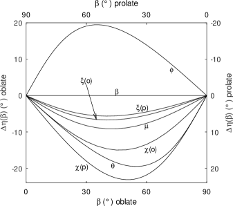
Figure 1: Auxiliary latitudes for oblate and prolate ellipsoids with $n=\pm\frac{1}{3}$. The quantities plotted are $\Delta\eta(\beta)=\eta(\beta)-\beta$ as a function of $\beta$ for $\eta=\phi$, $\beta$, $\theta$, $\mu$, $\chi$, and $\xi$. For the oblate ellipsoid, $n=\frac{1}{3}$, $a/b=2$, the scales are given by the bottom and left axes; for the prolate ellipsoid, $n=-\frac{1}{3}$, $a/b=\frac{1}{2}$, the scales are given by the reversed top and right axes. Because the values of $\lvert n\rvert$ are the same, the curves for the oblate and prolate cases coincide for the auxiliary latitudes, $\phi$, $\beta$, $\theta$, and $\mu$. For the other auxiliary latitudes, $\chi$ and $\xi$, the curves for the oblate and prolate cases are labeled with (o) and (p) respectively.

The behavior of $\Delta\eta(\beta)=\eta(\beta)-\beta$ as a function of $\beta$ is illustrated in Fig. 1 for an oblate ellipsoid $a/b=2$ and a prolate ellipsoid $a/b=\frac{1}{2}$; here $\eta$ stands for any of the auxiliary latitudes. This shows the symmetry in the behavior for $\phi$, $\beta$, $\theta$, and $\mu$, when $a$ and $b$ are interchanged; this follows from the observation that the relations between these auxiliary latitudes depend only on the properties of the meridian ellipse (as opposed to the ellipsoid). Also, because of the symmetric relationship of $\phi$ and $\theta$ with $\beta$, the curves, $\Delta\phi(\beta)$ and $\Delta\theta(\beta)$, are congruent.

3 Series expansions

The conversions between $\phi$, $\beta$, and $\theta$ are straightforward. However, the definition of $\mu$ involves a special function and none of the expressions for $\mu$, $\chi$, or $\xi$ can be inverted in closed form. As a consequence, many authors have obtained approximate expressions for the conversions based on the fact that the flattening of the earth ellipsoid is small. In this section, we examine this approach. Here we pick the third flattening $n$ as the expansion parameter. Some authors use $e^{2}$ instead; however, as we show in Sec. 7, this results in a much larger truncation error for all the conversions.

Let’s start by establishing a uniform and compact notation for the series. Take, for example, the series to convert $\phi$ to $\chi$ given by Krüger (1912, Eq. 5.8),

$$\chi(\phi)-\phi \textstyle=-\bigl{(}2n-\frac{2}{3}n^{2}-\frac{4}{3}n^{3}+\frac{82}{45}n^{4}\bigr{)}\sin 2\phi$$

$$\textstyle\quad{}+\bigl{(}\frac{5}{3}n^{2}-\frac{16}{15}n^{3}-\frac{13}{9}n^{4}\bigr{)}\sin 4\phi$$

$$\textstyle\quad{}-\bigl{(}\frac{26}{15}n^{3}-\frac{34}{21}n^{4}\bigr{)}\sin 6\phi$$

$$\textstyle\quad{}+\frac{1237}{630}n^{4}\sin 8\phi+\ldots.$$ (15)

This can be written as

$$\Delta\chi(\phi)=\mathbf{S}^{(4)}(\zeta)\cdot\mathsf{C}_{\chi\phi}^{(4\times 4)}\cdot\mathbf{P}^{(4)}(n)+O(n^{5}),$$ (16)

where

$$\mathbf{S}^{(L)}(\zeta)=[\sin 2\zeta,\sin 4\zeta,\sin 6\zeta,\ldots,\sin 2L\zeta]$$ (17)

is a row vector of length $L$,

$$\mathbf{P}^{(M)}(n)=[n,n^{2},n^{3},\ldots,n^{M}]^{\mathsf{T}}$$ (18)

is a column vector of length $M$, and

$$\mathsf{C}_{\chi\phi}^{(4\times 4)}=\begin{bmatrix}-2&\frac{2}{3}&\frac{4}{3}&-\frac{82}{45}\\ 0&\frac{5}{3}&-\frac{16}{15}&-\frac{13}{9}\\ 0&0&-\frac{26}{15}&\frac{34}{21}\\ 0&0&0&\frac{1237}{630}\end{bmatrix}$$ (19)

is an upper-triangular $4\times 4$ matrix. All of the conversions from one auxiliary latitude $\zeta$ to another $\eta$ follow the same pattern,

$$\Delta\eta(\zeta)=\mathbf{S}^{(L)}(\zeta)\cdot\mathsf{C}_{\eta\zeta}^{(L\times M)}\cdot\mathbf{P}^{(M)}(n)+O(n^{L+1}),$$ (20)

allowing us to represent each series by a single matrix $\mathsf{C}_{\eta\zeta}$. (Hereafter we will usually omit the $(L\times M)$ superscript on $\mathsf{C}_{\eta\zeta}$.) We stipulate $M\geq L$; if $M<L$, the last $L-M$ rows of $\mathsf{C}_{\eta\zeta}$ are zero—so it may be replaced by a $M\times M$ matrix. We can also write

$$\Delta\eta(\zeta) =\mathbf{S}^{(L)}(\zeta)\cdot\mathbf{F}_{\eta\zeta}^{(L\times M)}+O(n^{L+1})$$

$$=\sum_{l=1}^{L}F_{\eta\zeta,l}^{(L\times M)}\sin 2l\zeta+O(n^{L+1}),$$ (21)

where

$$\mathbf{F}_{\eta\zeta}^{(L\times M)}=C_{\eta\zeta}^{(L\times M)}\cdot\mathbf{P}^{(M)}(n)$$ (22)

is the length $L$ column vector of coefficients for the Fourier expansion of the periodic function $\Delta\eta(\zeta)$ truncated at order $n^{M}$. If $M\rightarrow\infty$, then $\mathbf{F}_{\eta\zeta}^{(L\times\infty)}$ gives the first $L$ exact Fourier coefficients provided that the series in $n$ converges (this question is addressed in Sec. 5). Usually we take $M=L$ as this defines the smallest matrix of coefficients which gives accuracy to order $n^{L}$.

Using a computer algebra system, it’s a simple matter to compute $\mathsf{C}_{\eta\zeta}$ for all $\eta$ and $\zeta$. I used Maxima (2022) which has embodied all the needed machinery (Taylor series, trigonometric simplification, integration) since at least the early 1970s. It also has the virtue of being freely available.

The Maxima code to produce these expansions is relatively straightforward and is included in the supplementary data for this paper. This uses the result of Delambre and Legendre (1799, p. 70) to give $\mathsf{C}_{\beta\phi}$ and the expansion given by Bessel (1825) for $s$ in terms of $\beta$,

$$s =\frac{a+b}{2}\biggl{(}B_{0}\beta+\sum_{l=1}^{\infty}\frac{B_{l}}{l}\sin 2l\beta\biggl{)},$$ (23)

$$B_{l} =\sum_{\begin{subarray}{c}j\geq l\\ j-l\text{ even}\end{subarray}}\frac{(j+l-3)!!\,(j-l-3)!!}{(j+l)!!\,(j-l)!!}n^{j},$$ (24)

as the starting point for $C_{\mu\beta}$. (Here $j!!$ is the double factorial extended to negative odd numbers so that $(-1)!!=1$ and $(-3)!!=-1$.) Series reversion was used to find $\mathsf{C}_{\zeta\eta}$ given $\mathsf{C}_{\eta\zeta}$. One series can be substituted in another to find $\mathsf{C}_{\eta\zeta}$ given $\mathsf{C}_{\eta\omega}$ and $\mathsf{C}_{\omega\zeta}$. In this way, all 30 non-trivial $\mathsf{C}_{\eta\zeta}$ can be found. These are listed for $M=L=6$ in Appendix A, Eqs. (62)–(89).

The series for all the conversions between the 4 latitudes $\phi$, $\beta$, $\theta$, and $\mu$ have alternating zeros in each row. This follows because interchanging $a$ and $b$, a symmetry exhibited in Fig. 1, changes the sign of $n$. This property of the expansions in $n$ was recognized by Bessel (1825); Helmert (1880); earlier, Euler (1755) used $e^{\prime\prime 2}$ which has the same property.

Some of these expansions truncated to lower order can be found in the literature. In particular, Krüger (1912) gives $\mathsf{C}_{\chi\phi}$, his Eq. 5.8; $\mathsf{C}_{\phi\chi}$, Eq. 5.9; $\mathsf{C}_{\chi\mu}$, Eq. 7.26*; and $\mathsf{C}_{\mu\chi}$, Eq. 8.41. These series suffice to generalize the spherical transverse Mercator projection to the ellipsoid. Similarly Helmert (1880), in his treatment of geodesics, gives $\mathsf{C}_{\mu\beta}$, his Eq. 5.5.7; and $\mathsf{C}_{\beta\mu}$, Eq. 5.6.8.

4 Truncation errors

Modern geodetic libraries should strive to achieve full double-precision accuracy. This can be obtained at minimal cost and ensures that the libraries continue to be relevant as geodetic measurements become more precise. As a starting point, consider the truncation errors for the series expansions with $M=L=5$; as we shall see this gives accurate results for terrestrial ellipsoids, exemplified by the International Ellipsoid 1924, with $f=1/297$. The error in evaluating $\Delta\eta(\zeta)$ is

$$\delta_{\eta\zeta}(\zeta)=\mathbf{S}(\zeta)\cdot\bigl{(}\mathsf{C}_{\eta\zeta}^{(L\times L)}-\mathsf{C}_{\eta\zeta}^{(16\times 16)}\bigr{)}\cdot\mathbf{P}(n),$$ (25)

where we assume that the results with $M=L=16$ are fully converged. After the subtraction, the resulting matrix is $\mathsf{C}_{\eta\zeta}^{(16\times 16)}$ with the first $L=5$ columns set to zero. In this way, we can compute the truncation error using double-precision arithmetic without the competing effects of roundoff.

Table 3: Absolute (a) and relative (b) truncation errors of the series expansions in $n$ for $f=1/297$, truncated at $M=L=5$. Here and in the following tables, the errors are measured in ulps defined as $2^{-53}\,\mathrm{radian}$ for the absolute errors and 1 part in $2^{53}$ for the relative errors. The results are given consistently to 2 significant figures.

(a)

$\eta\backslash\zeta$	$\phi$	$\beta$	$\theta$	$\mu$	$\chi$	$\xi$
$\phi$	$-$	$0.035$	$6$	$2.3$	$17$	$1.1$
$\beta$	$0.035$	$-$	$0.035$	$0.35$	$3.4$	$0.15$
$\theta$	$6$	$0.035$	$-$	$0.23$	$1.9$	$0.11$
$\mu$	$0.18$	$0.0024$	$0.67$	$-$	$0.86$	$0.018$
$\chi$	$2.1$	$0.11$	$0.56$	$0.11$	$-$	$0.079$
$\xi$	$0.086$	$0.0039$	$0.75$	$0.058$	$1.5$	$-$

(b)

$\eta\backslash\zeta$	$\phi$	$\beta$	$\theta$	$\mu$	$\chi$	$\xi$
$\phi$	$-$	$0.41$	$13$	$4.9$	$40$	$2.5$
$\beta$	$0.41$	$-$	$0.41$	$0.73$	$12$	$0.3$
$\theta$	$13$	$0.41$	$-$	$0.49$	$3.8$	$0.33$
$\mu$	$0.66$	$0.0051$	$1.4$	$-$	$4.6$	$0.037$
$\chi$	$5.9$	$0.41$	$1.2$	$0.43$	$-$	$0.33$
$\xi$	$0.58$	$0.0086$	$1.6$	$0.12$	$6.9$	$-$

Table 4: Absolute (a) and relative (b) truncation errors of the series expansions in $n$ for $f=1/150$, truncated at $M=L=6$. To obtain the corresponding values for other (small) values of $f$, multiply the figures in this table by $(150f)^{7}$; e.g., the truncation errors for $f=1/300$ are a factor $128$ smaller.

(a)

$\eta\backslash\zeta$	$\phi$	$\beta$	$\theta$	$\mu$	$\chi$	$\xi$
$\phi$	$-$	$0.006$	$2.9$	$0.98$	$9$	$0.34$
$\beta$	$0.006$	$-$	$0.006$	$0.13$	$1.7$	$0.04$
$\theta$	$2.9$	$0.006$	$-$	$0.099$	$0.87$	$0.04$
$\mu$	$0.037$	$0.00069$	$0.24$	$-$	$0.31$	$0.0043$
$\chi$	$0.78$	$0.018$	$0.18$	$0.022$	$-$	$0.023$
$\xi$	$0.015$	$0.00042$	$0.28$	$0.015$	$0.6$	$-$

(b)

$\eta\backslash\zeta$	$\phi$	$\beta$	$\theta$	$\mu$	$\chi$	$\xi$
$\phi$	$-$	$0.085$	$5.8$	$2$	$20$	$0.74$
$\beta$	$0.085$	$-$	$0.085$	$0.27$	$4.1$	$0.09$
$\theta$	$5.8$	$0.085$	$-$	$0.2$	$1.9$	$0.079$
$\mu$	$0.13$	$0.0014$	$0.49$	$-$	$1.5$	$0.0085$
$\chi$	$1.7$	$0.085$	$0.36$	$0.055$	$-$	$0.066$
$\xi$	$0.12$	$0.00099$	$0.56$	$0.033$	$2.3$	$-$

The absolute truncation error is just the maximum value of $\lvert\delta_{\eta\zeta}(\zeta)\rvert$ as $\zeta$ is varied. Table 3(a) gives these absolute errors for this case and Table 4(a) gives the corresponding values for $M=L=6$ and $f=1/150$; this is the value of $f$ for the SRMmax ellipsoid used by the US National Geospatial-Intelligence Agency to “stress test” projection libraries. The errors are reported in “ulps”, units in the last place; for the purpose of measuring the absolute error of latitudes, we define $1\,\mathrm{ulp}=2^{-53}\,\mathrm{radian}$. (Standard double-precision hardware provides 53 bits of precision.) Thus, values less than $1\,\mathrm{ulp}$ mean that the truncation error is less than the roundoff error and values in the range $1\,\mathrm{ulp}$–$8\,\mathrm{ulp}$ mean that the truncation error is comparable to the roundoff error. We see that the series truncated at $n^{5}$ are usually satisfactory for $f=1/297$; however, for production use, it is wise to use the series truncated at $n^{6}$ (listed in Appendix A) which give accurate results even for $f=1/150$.

In mapping applications, it is necessary to apply a more stringent error metric, namely that the relative error in the latitude or the colatitude be small. For example, the radial coordinate of the polar stereographic projection is proportional to $\rho_{\chi}=2\tan\frac{1}{2}\chi^{\prime}$, where the prime is used to signify the colatitude; in order to preserve accuracy at the pole, the relative error in $\chi^{\prime}$ must be small. These requirements can be met by representing the latitude by its tangent because $\tan\eta$ can accurately represent angles extremely close to $0$ and to $\pm\frac{1}{2}\pi$. Thus, $\rho_{\chi}$ can be expressed as

$$\rho_{\chi}=2\Bigl{(}\sqrt{1+\tan^{2}\chi}\pm\tan\chi\Bigr{)}^{\mp 1},$$ (26)

for $\chi\gtrless 0$. Similarly, the radial coordinate for the Lambert equal-area projection is proportional to $\rho_{\xi}=2\sin\frac{1}{2}\xi^{\prime}$ and this can be evaluated as

$$\rho_{\xi}=\sqrt{2\Bigl{(}\sqrt{1+\tan^{2}\xi}\pm\tan\xi\Bigr{)}^{\mp 1}\Big{/}\sqrt{1+\tan^{2}\xi}},$$ (27)

for $\xi\gtrless 0$. This replaces the ill-conditioned expression, $\sqrt{A_{p}-A}$, given by Snyder (1987, Eq. 24-23). To determine the relative error in $\tan\eta$, we multiply the absolute error by $\mathrm{d}\log\tan\eta/\mathrm{d}\eta=1/(\sin\eta\cos\eta)$. This measure of the relative error is given in Tables 3(b) and 4(b); now, for the purposes of measuring the relative error, we define $1\,\mathrm{ulp}$ to be 1 part in $2^{53}$. Because the maximum value of $\sin\eta\cos\eta$ is $\frac{1}{2}$, the relative errors are all at least twice as large as the absolute errors.

Table 5: Absolute (a) and relative (b) truncation errors of the exact Fourier series ($M\rightarrow\infty$) for $f=1/150$, truncated at $L=6$.

(a)

$\eta\backslash\zeta$	$\phi$	$\beta$	$\theta$	$\mu$	$\chi$	$\xi$
$\phi$	$-$	$0.006$	$0.78$	$0.32$	$2.4$	$0.13$
$\beta$	$0.006$	$-$	$0.006$	$0.038$	$0.41$	$0.012$
$\theta$	$0.78$	$0.006$	$-$	$0.016$	$0.18$	$0.0046$
$\mu$	$0.019$	$0.000097$	$0.057$	$-$	$0.046$	$0.00069$
$\chi$	$0.15$	$0.000093$	$0.031$	$0.0017$	$-$	$0.00084$
$\xi$	$0.011$	$0.00014$	$0.065$	$0.0031$	$0.095$	$-$

(b)

$\eta\backslash\zeta$	$\phi$	$\beta$	$\theta$	$\mu$	$\chi$	$\xi$
$\phi$	$-$	$0.085$	$11$	$4.4$	$33$	$1.8$
$\beta$	$0.085$	$-$	$0.085$	$0.53$	$5.7$	$0.17$
$\theta$	$11$	$0.085$	$-$	$0.23$	$2.5$	$0.065$
$\mu$	$0.27$	$0.0014$	$0.8$	$-$	$0.64$	$0.0096$
$\chi$	$2.1$	$0.0013$	$0.43$	$0.024$	$-$	$0.012$
$\xi$	$0.15$	$0.0019$	$0.9$	$0.043$	$1.3$	$-$

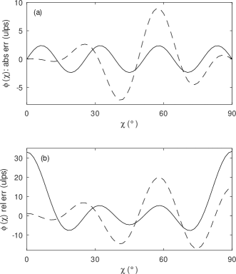
Figure 2: Absolute (a) and relative (b) errors in computing $\phi(\chi)$ with the expansions in $n$. Here we have $f=1/150$ and $L=6$ harmonics are included; the solid (resp. dashed) lines correspond to keeping $M\rightarrow\infty$ (resp. $M=6$) terms in the Taylor series expansions for the Fourier coefficients.

So far, we have investigated the truncation error with $M=L$ which corresponds to a consistent truncation to order $n^{L}$. Since the vector of Fourier coefficients $\mathbf{F}_{\eta\zeta}^{(L\times M)}$, Eq. (22), can be computed once the flattening of the ellipsoid is known, it might be worthwhile to choose $M>L$ so that the vector more closely approximates the exact Fourier coefficients. For example, with $L=6$ and $M=16$, we have a fully converged result for each Fourier coefficient for $f=1/150$. The truncation error is now computed using $\bigl{(}\mathsf{C}_{\eta\zeta}^{(L\times 16)}-\mathsf{C}_{\eta\zeta}^{(16\times 16)}\bigr{)}$ which is the same as setting the first $L=6$ rows of $\mathsf{C}_{\eta\zeta}^{(16\times 16)}$ to zero. Table 5 shows these truncation errors. As expected, all the absolute errors, Table 5(a), are less than or equal to the corresponding values in Table 4(a). On the other hand, the relative errors in Table 5(b) are, in many cases, greater than the values in Table 4(b); adding more terms in the expansions for the Fourier coefficients leads to a less accurate result (as judged by the relative error). This somewhat surprising result is explained by Fig. 2 for the case of $\phi(\chi)$: The error in the Fourier series with the exact coefficients, approximately given by the next term in the Fourier series, oscillates sinusoidally as a function of $\zeta$; in this way the Fourier series effectively minimizes the maximum absolute error; see the solid line in Fig. 2(a). By the same token, this leads to an increase in the relative error near $\zeta=0$ and $\frac{1}{2}\pi$ where $\sin\eta\cos\eta$ is small; see the solid line in Fig. 2(b). The dashed lines in this figure give the errors with the Fourier coefficients truncated at $M=6$.

5 Radii of convergence

The series expansions given here offer accurate conversions between auxiliary latitudes for most geodetic applications. As the eccentricity increases, it is possible to add additional terms to the series so that accurate results are still obtained. However, this becomes increasingly fruitless for $\lvert f\rvert\gtrsim\frac{1}{10}$. Generating the coefficients $\mathsf{C}_{\eta\zeta}^{(L\times L)}$ becomes impractical for $L>20$, but more seriously, the series stop converging for $\lvert n\rvert\geq r_{\eta\zeta}$, the “radius of convergence”. For some conversions, e.g., $\mathsf{C}_{\beta\phi}$, the radius of convergence is, from the behavior of the coefficients in Eq. (62), $r_{\beta\phi}=1$; i.e., the series converges for all possible eccentricities; but for other conversions the radius of convergence is considerably narrower.

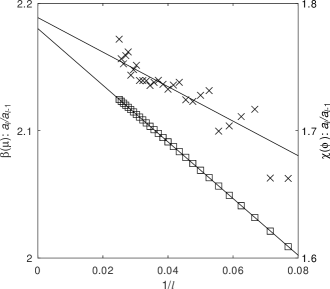
Figure 3: Domb-Sykes plots to determine the convergence for the series expansions in $n$ for $\beta(\mu)$ (squares, scale on left) and $\chi(\phi)$ (crosses, scale on right). The lines give the least-squares linear fits to the 20 points with $20<l\leq 40$. The intercepts of the linear fits at $1/l\rightarrow 0$ provide estimates of $1/r_{\beta\mu}$ and $1/r_{\chi\phi}$.

Table 6: Radii of convergence, $r_{\eta\zeta}$, for the expansions in $n$. The values listed as “1” are exact. The other values are given with as many (up to 7) decimal places as are consistent with the several fits to $a_{l}/a_{l-1}$. Thus, the value $r_{\beta\mu}=0.459$ means that the estimates all round to this result with 3 decimal places, but not with 4 decimal places. If the result isn’t unique with 2 decimal places, then the range of values is given. Thus, the certainty of the estimate of $r_{\eta\zeta}$ is given by the number of decimal places shown or by the range given. In some cases, e.g., $r_{\mu\beta}$, the range includes impossible values greater than unity; this just reflects the uncertainty of the fits. The values for $r_{\theta\phi}$ and $r_{\phi\theta}$ are very close to $\sqrt{2}-1$; presumably this result could be established rigorously.

$\eta\backslash\zeta$	$\phi$	$\beta$	$\theta$	$\mu$	$\chi$	$\xi$
$\phi$	$-$	1	0.4142136	0.4587	0.32–0.35	0.52
$\beta$	1	$-$	1	0.459	0.31–0.35	0.52–0.53
$\theta$	0.4142136	1	$-$	0.4590	0.33–0.34	0.51–0.53
$\mu$	1.00	0.83–1.28	0.41	$-$	0.32–0.34	0.52–0.56
$\chi$	0.54–0.57	0.75–1.43	0.41	0.46	$-$	0.51–0.57
$\xi$	1.00–1.01	0.99–1.00	0.41	0.46	0.33–0.35	$-$

A sufficient condition for convergence is that $\lim_{L\rightarrow\infty}\sum_{l=1}^{L}a_{l}n^{l}$ is finite, where $a_{l}$ is the sum of the absolute values of the $l$th column of $\mathsf{C}$ (we temporally drop the subscripts $\eta\zeta$). The radius of convergence is then $r=\lim_{l\rightarrow\infty}a_{l-1}/a_{l}$. We generated $\mathsf{C}^{(40\times 40)}$ using Maxima (2022), and so could obtain $a_{l}$ for $l\leq 40$. We can estimate $r$ using the Domb and Sykes (1957) method, i.e., finding $r$ and $B$ which gives the least-squares linear fit for $a_{l}/a_{l-1}\approx 1/r+B/l$. We used the 20 values $l=21$ through $40$ for the fit and we checked its soundness by using several subsets of 10 out of the 20 points. In some cases, the fit is unambiguous, see the squares in Fig. 3 for the conversion $\beta(\mu)$. In others, the various fits yield different values of $r$, see the crosses in the same figure for the conversion $\chi(\phi)$. The results are summarized in Table 6. The smallest radii of convergence $r_{\eta\chi}$ are about $\frac{1}{3}$; i.e., convergence for $\frac{1}{2}\lesssim b/a\lesssim 2$ or $-1\lesssim f\lesssim\frac{1}{2}$.

6 Evaluating the series

Once the ellipsoid is selected, i.e., $n$ is known, then the vector of Fourier coefficients $\mathbf{F}_{\eta\zeta}^{(L\times M)}$, Eq. (22), can be evaluated. Each coefficient is given as a polynomial of order $M$ in $n$ and so can be evaluated rapidly and accurately using the Horner method. This evaluation should account for the fact that the leading term in $F_{\eta\zeta,l}^{(L\times M)}$ is $O(n^{l})$. Also, the polynomials for the conversions between $\phi$, $\beta$, $\theta$, and $\mu$ are, because of the alternating zeros, in $n^{2}$ rather than in $n$.

We are then left with the evaluation of the sums of the form

$$\Delta\eta(\zeta)=\sum_{l=1}^{L}F_{\eta\zeta,l}^{(L\times M)}\sin 2l\zeta.$$ (28)

These are most conveniently evaluated using Clenshaw (1955) summation. Although the method is well known, several software libraries use more cumbersome methods for the summation. So let us review the method and reintroduce some less well known optimizations that may be important in reducing roundoff errors. We consider the more general series

$$p(\zeta)=\sum_{k=0}^{K-1}c_{k}f_{k}(\zeta),$$ (29)

where

$$f_{k}(\zeta)=\sin\bigl{(}2(k+k_{0})\zeta+\zeta_{0}\bigl{)}.$$ (30)

Equation 28 is the special case $k_{0}=1$, $\zeta_{0}=0$, $c_{k}=F_{\eta\zeta,k+1}^{(L\times M)}$ with $k=l-1$. The general form of $f_{k}(\zeta)$ satisfies

$$f_{k-1}(\zeta)+f_{k+1}(\zeta)=2xf_{k}(\zeta),$$ (31)

where $x=(\cos\zeta+\sin\zeta)(\cos\zeta-\sin\zeta)$. Clenshaw summation then proceeds as follows:

$$u_{K+1} =u_{K}=0,$$ (32)

$$u_{k} =2xu_{k+1}-u_{k+2}+c_{k},\quad\text{for $K>k\geq 0$},$$ (33)

$$p(\zeta) =u_{0}f_{0}(\zeta)-u_{1}f_{-1}(\zeta).$$ (34)

Note that the method involves no additional computation of trigonometric functions beyond $\sin\zeta$ and $\cos\zeta$. As with the Horner method, the sum is computed starting with the highest-order (smallest) terms and thus roundoff errors are minimized; in addition, the leading coefficient in $p(\zeta)$, $c_{0}$, is $O(n)$ which further reduces the impact of roundoff errors.

Evaluating the series for auxiliary latitudes, $f_{k}(\zeta)=\sin\bigl{(}2(k+1)\zeta\bigl{)}$, we have $p(\zeta)=2u_{0}\sin\zeta\cos\zeta$. Because this product includes $\sin\zeta$ and $\cos\zeta$, the relative error due to roundoff is also small when evaluating $\eta(\zeta)$ both near the equator ($\sin\zeta$ small) and near a pole ($\cos\zeta$ small).

It is important to stress that, for the general case of Clenshaw summation (with arbitrary $c_{k}$), the computation may be unstable if $\sin\zeta$ or $\cos\zeta$ is small. This is not the case when $c_{k}$ is strongly decreasing—the situation in our application. However, for completeness, here is the modification (Oliver, 1977, Reinsch, unpublished) needed in these cases:

$$x\mp 1 =\begin{cases}-2\sin^{2}\zeta,&\text{for upper sign, if $\lvert\sin\zeta\rvert$ small},\\ 2\cos^{2}\zeta,&\text{for lower sign, if $\lvert\cos\zeta\rvert$ small},\end{cases}$$ (35)

$$d_{K} =u_{K+1}=u_{K}=0,$$ (36)

$$d_{k} =2(x\mp 1)u_{k+1}\pm d_{k+1}+c_{k},\quad\text{for $K>k\geq 0$},$$ (37)

$$u_{k} =d_{k}\pm u_{k+1},\quad\text{for $K>k\geq 0$},$$ (38)

$$p(\zeta) =u_{0}f_{0}(\zeta)-u_{1}f_{-1}(\zeta).$$ (39)

Snyder (1987, §3) writes the trigonometric series, Eq. (28), as a power series in $x$. This also avoids multiple calls to trigonometric functions, but entails manipulating the coefficients of the series. Clenshaw summation offers a more straightforward approach.

7 Expanding in other small parameters

As mentioned at the beginning of Sec. 3, some authors use the eccentricity squared, $e^{2}$, as the expansion parameter instead of $n$. It is rather simple to generate the resulting series. Express $n$ in terms of $e^{2}$,

$$n=\frac{1-\sqrt{1-e^{2}}}{1+\sqrt{1-e^{2}}}=\frac{1}{4}e^{2}+\frac{1}{8}e^{4}+\frac{5}{64}e^{6}+\ldots.$$ (40)

We can then write

$$\mathbf{P}(n)=\mathsf{T}(n,e^{2})\cdot\mathbf{P}(e^{2}),$$ (41)

where $\mathsf{T}(n,e^{2})$ is an $M\times M$ matrix whose $m$th row consists of the coefficients of the expansion of $n^{m}$ in terms of $e^{2}$. Substituting in Eq. (20), we obtain

$$\Delta\eta(\zeta)=\mathbf{S}(\zeta)\cdot\mathsf{C}_{\eta\zeta}\cdot\mathsf{T}(n,e^{2})\cdot\mathbf{P}(e^{2})+O(n^{L+1}).$$ (42)

Thus $\mathsf{C}_{\eta\zeta}\cdot\mathsf{T}(n,e^{2})$ provides the matrix of coefficients for the expansion in $e^{2}$.

Table 7: Absolute (a) and relative (b) truncation errors of the series expansions in $e^{2}$ for $f=1/150$, truncated at $M=L=6$.

(a)

$\eta\backslash\zeta$	$\phi$	$\beta$	$\theta$	$\mu$	$\chi$	$\xi$
$\phi$	$-$	$28$	$82$	$59$	$71$	$53$
$\beta$	$28$	$-$	$28$	$12$	$16$	$10$
$\theta$	$82$	$28$	$-$	$23$	$23$	$23$
$\mu$	$41$	$5.8$	$30$	$-$	$1.2$	$0.54$
$\chi$	$43$	$3.7$	$31$	$0.56$	$-$	$0.53$
$\xi$	$39$	$6.3$	$28$	$0.79$	$1.9$	$-$

(b)

$\eta\backslash\zeta$	$\phi$	$\beta$	$\theta$	$\mu$	$\chi$	$\xi$
$\phi$	$-$	$140$	$660$	$440$	$660$	$350$
$\beta$	$140$	$-$	$140$	$83$	$140$	$62$
$\theta$	$660$	$140$	$-$	$83$	$65$	$93$
$\mu$	$230$	$19$	$68$	$-$	$7.8$	$3.4$
$\chi$	$300$	$11$	$68$	$2.3$	$-$	$3.4$
$\xi$	$200$	$22$	$67$	$5.8$	$20$	$-$

The transformation matrix $\mathsf{T}(n,e^{2})$ is given by Eq. (90) and an example of the expansion in $e^{2}$ (for converting from $\phi$ to $\mu$) is given by Eq. (91). Comparing this with Eq. (66), we note that the series in terms of $e^{2}$ has lost the nice property of alternating zeros. More damning, the truncation errors for the expansions in $e^{2}$, Table 7, are all much worse, in many cases by factors in excess of 100, than for the corresponding expansions in $n$; compare Table 4.

In light of this, the only reason to wish to convert a series in $n$ into the corresponding series in $e^{2}$ is to confirm that the truncation error is larger and to cross-check the results with publications that use this expansion. However, the same technique can be profitably used to convert an arbitrary series in $e^{2}$ to one in $n$: just multiply the matrix of coefficients for the $e^{2}$ series by $\mathsf{T}(e^{2},n)$ which is the matrix inverse of $\mathsf{T}(n,e^{2})$, Eq. (92).

The procedure outlined here to obtain the series in $e^{2}$ can, of course, be applied for any of the small parameters listed in Table 2. The resulting matrices, $\mathsf{T}(n,\ldots)$, are included in the supplementary data. Besides $n$, the only parameter with comparably small truncation errors is the third eccentricity squared, $e^{\prime\prime 2}$, the choice of Euler (1755). Additionally, we remark that the series for converting between $\phi$ and $\theta$ is simpler using $e^{\prime\prime 2}$ compared to $n$; for example, we have $\mathsf{C}_{\theta\phi}\cdot\mathsf{T}(n,e^{\prime\prime 2})=\mathsf{C}_{\beta\phi}$, a diagonal matrix (Adams, 1921, p. 13).

8 Direct evaluation of latitudes

The 6th-order series given in Appendix A provides full double-precision accuracy for $\lvert f\rvert\leq 1/150$. For $f$ outside this range, we can add more terms to the series to maintain the accuracy. For example, the 8th-order series, $M=L=8$, are needed for $\lvert f\rvert\leq 1/50$. However, even though extending the series to 40th order is feasible (see the supplementary data), going beyond 12th order, say, is impractical: the number of coefficients become large increasing the size of the program and the time to compute the latitudes. Furthermore, as we saw in Sec. 5, some of the series cease to converge for large $\lvert f\rvert$.

In those cases where using the series is not feasible, we can convert between the auxiliary latitudes using the defining relations given in Sec. 2. (Regardless of the value of $f$, this approach is also recommended for the conversions between $\phi$, $\beta$, and $\theta$.) In order to ensure that the conversions maintain full accuracy even at the equator and at the poles, we cast the relations in terms of the tangents of the angles and demand that the relative roundoff errors are small. The relations for $\beta$ and $\theta$ are simple

$$\tan\beta =(1-f)\tan\phi,$$ (43)

$$\tan\theta =(1-f)^{2}\tan\phi.$$ (44)

Given $\beta$, we can find $\mu$ using Eqs. (6) and (7); however, these equations by themselves will not yield good relative accuracy near the pole. This is fixed by computing not only $s$, the meridian distance from the equator, but also $s^{\prime}=s_{p}-s$, the distance from the pole, using

$$s^{\prime}=aE(\beta^{\prime},e).$$ (45)

Then we have

$$\tan\mu=\frac{\sin\bigl{(}\frac{1}{2}\pi s/s_{p}\bigl{)}}{\sin\bigl{(}\frac{1}{2}\pi s^{\prime}/s_{p}\bigl{)}}.$$ (46)

(This assumes that $\beta\geq 0$. A similar equation can be written for $\beta<0$.) The elliptic functions can be evaluated with

$$E(\zeta,k) =\sin\zeta\bigl{(}R_{F}(\cos^{2}\zeta,1-k^{2}\sin^{2}\zeta,1)$$

$$\quad{}-\textstyle\frac{1}{3}k^{2}\sin^{2}\zeta\,R_{D}(\cos^{2}\zeta,1-k^{2}\sin^{2}\zeta,1)\bigr{)},$$ (47)

for $k^{2}\leq 0$, and

$$E(\zeta,k) =\sin\zeta\bigl{(}k^{\prime 2}\,R_{F}(\cos^{2}\zeta,k^{\prime 2}+k^{2}\cos^{2}\zeta,1)$$

$$\quad{}+\textstyle\frac{1}{3}k^{2}k^{\prime 2}\sin^{2}\zeta\,R_{D}(\cos^{2}\zeta,1,k^{\prime 2}+k^{2}\cos^{2}\zeta)$$

$$\quad{}+k^{2}\cos\zeta/\sqrt{k^{\prime 2}+k^{2}\cos^{2}\zeta}\bigr{)},$$ (48)

where $k^{\prime 2}=1-k^{2}$, for $0\leq k^{2}\leq 1$. These results assume that $\lvert\zeta\rvert\leq\frac{1}{2}\pi$. The functions $R_{F}(x,y,z)$, $R_{D}(x,y,z)$, and $R_{G}(x,y,z)$ (used below) are symmetric elliptic integrals defined in Olver et al. (2010, §http://dlmf.nist.gov/19.16.i) which can be numerically evaluated to arbitrary precision using Carlson (1995); see also Olver et al. (2010, §http://dlmf.nist.gov/19.36.i)

The conditions on $k^{2}$ for Eqs. (47) and (48) ensure that the terms on the right hand sides are all positive thus minimizing the roundoff error. For an oblate (resp. prolate) ellipsoid, we would compute $s=bE(\beta,ie^{\prime})$ with Eq. (47) (resp. Eq. (48)) and $s^{\prime}=bE(\beta^{\prime},e)$ with Eq. (48) (resp. Eq. (47)). The quarter meridian can be computed with (Olver et al., 2010, Eq. http://dlmf.nist.gov/19.25.E1)

$$s_{p}=aE(e)=bE(ie^{\prime})=2R_{G}(0,a^{2},b^{2});$$ (49)

however, in practice, it is simpler to use $s_{p}=s+s^{\prime}$.

Equations (47) and (48) are obtained from Eqs. 19.25.9 and 19.25.10 from Olver et al. (2010, §http://dlmf.nist.gov/19.25.i). However, the term $\sin\zeta$ has been factored out of each equation. This ensures good relative accuracy when $\sin\zeta$ is small and this, in turn, ensures high accuracy for Eq. (46) when either $\sin\beta$ or $\cos\beta=\sin\beta^{\prime}$ is small.

For treating the conformal latitude, we use the formulation of Karney (2011) combining Eqs. (8) and (10) to give

$$\tan\chi=\tan\phi\sqrt{1+\sigma(\sin\phi)^{2}}-\sigma(\sin\phi)\sqrt{1+\tan^{2}\phi},$$ (50)

where

$$\sigma(x)=\sinh\bigl{(}e\tanh^{-1}(ex)\bigr{)}.$$ (51)

Finally, we consider the equation for $\xi$, Eq. (14). Since this equation specifies just the sine of $\xi$, it results in a huge absolute error when evaluated numerically near a pole; this results in a distance error of about $0.1\,\mathrm{m}$ on a terrestrial ellipsoid. The fix is to write the expression for $\cos\xi=\sqrt{1-\sin^{2}\xi}$ and then manipulate the result to avoid large cancellations. This process gives

$$\tan\xi=\frac{q(\sin\phi)}{\cos\phi\sqrt{\mathord{\ooalign{$\triangle$\cr\hfil$\mid$\hfil\cr}}[q](1,\sin\phi)\mathord{\ooalign{$\triangle$\cr\hfil$\mid$\hfil\cr}}[q](1,-\sin\phi)}},$$ (52)

where

$$q(x)=\frac{\tanh^{-1}(ex)}{e}+\frac{x}{1-e^{2}x^{2}},$$ (53)

and $\mathord{\ooalign{$\triangle$\cr\hfil$\mid$\hfil\cr}}[q](x,y)$ is its “divided difference”,

$$\mathord{\ooalign{$\triangle$\cr\hfil$\mid$\hfil\cr}}[q](x,y)=\begin{cases}\displaystyle\frac{q(y)-q(x)}{y-x},&\text{for $xy<0$},\\[8.61108pt] \displaystyle\frac{\mathrm{d}q(x)}{\mathrm{d}x}=\frac{2}{(1-e^{2}x^{2})^{2}},&\text{for $y=x$},\\[8.61108pt] \displaystyle\frac{1}{e(y-x)}\tanh^{-1}\frac{e(y-x)}{1-e^{2}xy}\\[8.61108pt] \quad\displaystyle{}+\frac{1+e^{2}xy}{(1-e^{2}x^{2})(1-e^{2}y^{2})},&\text{otherwise}.\end{cases}$$ (54)

The first of these expressions for $\mathord{\ooalign{$\triangle$\cr\hfil$\mid$\hfil\cr}}[q](x,y)$ is the defining relationship of the divided difference and this can be evaluated without excessive roundoff if $x$ and $y$ have opposite signs; the second is the result of taking the limit $y\rightarrow x$; and the final one is obtained using the results of Kahan and Fateman (1999) and gives accurate results even when $y\approx x$.

Equations (43), (44), (46), (50), and (52), allow $\phi$ to be converted to the other five auxiliary latitudes (with an intermediate conversion to $\beta$ required for the conversion to $\mu$). Equations (43) and (44) can be trivially inverted to give $\phi$ in terms of $\beta$ or $\theta$.

The other equations cannot be inverted in closed form and for these we use Newton’s method to obtain an accurate result with just a few iterations. This method requires knowledge of the derivatives $\mathrm{d}\tan\eta/\mathrm{d}\tan\phi$ which we list here:

$$\frac{\mathrm{d}\tan\mu}{\mathrm{d}\tan\phi} =\frac{\pi}{2}\frac{(1-f)^{2}}{E(e)}\frac{\cos^{3}\beta}{\cos\phi\cos^{2}\mu},$$ (55)

$$\frac{\mathrm{d}\tan\chi}{\mathrm{d}\tan\phi} =(1-f)^{2}\frac{\cos^{2}\beta}{\cos\chi\cos\phi},$$ (56)

$$\frac{\mathrm{d}\tan\xi}{\mathrm{d}\tan\phi} =\frac{2}{q(1)}\frac{\cos^{4}\beta}{\cos^{3}\xi\cos\phi}.$$ (57)

We can easily take the limit, $\phi\rightarrow 0$: merely replace the cosine terms by unity. In the limit, $\phi\rightarrow\frac{1}{2}\pi$, we have

$$\frac{\mathrm{d}\tan\mu}{\mathrm{d}\tan\phi} \rightarrow\frac{2}{\pi}(1-f){E(e)},$$ (58)

$$\frac{\mathrm{d}\tan\chi}{\mathrm{d}\tan\phi} \rightarrow\sqrt{1+\sigma(1)^{2}}-\sigma(1),$$ (59)

$$\frac{\mathrm{d}\tan\xi}{\mathrm{d}\tan\phi} \rightarrow(1-f)^{2}\sqrt{\frac{q(1)}{2}}.$$ (60)

Suitable starting guesses for $\tan\phi$ are $\tan\mu/({1-f})^{3/2}$, $\tan\chi/({1-f})^{2}$, or $\tan\xi/({1-f})^{4/3}$; these are accurate guesses for small $f$.

9 Implementation

The supplementary data for this paper includes a model C++ implementation of the methods described here. The class AuxAngle is a simple class that enables representation of an angle by a point in a two-dimensional plane and this facilitates algorithms written in terms of the tangent of the angle. The class AuxLatitude implements the conversions between all six auxiliary latitudes with the option of using either the series expansions or the direct evaluation of the equations for the latitudes. The order of the series expansions can be selected at compile time to be either $4$, $6$ (the default), or $8$.

The implementation allows the arithmetic to be carried out either at standard double precision or using arbitrary precision arithmetic using the MPREAL C++ interface (Holoborodko, 2022) to the MPFR library (Fousse et al., 2007). This provides an alternative method of computing the truncation errors given in Sec. 4: merely evaluate, at high precision, the differences of the auxiliary latitudes evaluated using the series method and the direct method. This serves as a confirmation that both methods are correctly coded.

However, the more interesting capability is the accurate measurement of the roundoff errors for both the series and the direct evaluation methods. This can be straightforwardly accomplished by taking the difference of the results of the double-precision and high-precision calculations. For the 6th-order series method, the absolute (resp. relative) roundoff error is about $2\,\mathrm{ulp}$ (resp. $4\,\mathrm{ulp}$). These errors should be added to the truncation errors in Table 4, scaled by $(150f)^{7}$.

Controlling the roundoff errors for the direct method is more challenging. We require, somewhat arbitrarily, an absolute error of no more than $10\,\mathrm{ulp}$ (equivalent to about $7\,\mathrm{nm}$ in the terrestrial ellipsoid) and a relative error of no more than $30\,\mathrm{ulp}$; we limited the testing to $\lvert n\rvert\leq 0.99$. By this criterion, the formulas given in Sec. 8 for converting from $\phi$ to $\beta$, $\theta$, and $\mu$, are accurate for the full range of $n$ tested. However, conversions from $\phi$ to $\chi$ and $\xi$ are only accurate for $-0.69\leq n\leq 0.40$. We are able to extend the region of accuracy for prolate ellipsoids by adapting the formulas somewhat. For example, we use

$$\frac{\tanh^{-1}(e\sin\phi)}{e}=\begin{cases}\displaystyle\frac{\tan^{-1}(\sqrt{-e^{2}}\sin\phi)}{\sqrt{-e^{2}}},&\text{for $f<0$},\\ \sin\phi,&\text{for $f=0$},\\[4.30554pt] \displaystyle\frac{\sinh^{-1}(e^{\prime}\sin\beta)}{e},&\text{for $f>0$}.\end{cases}$$ (61)

The expressions for $f\leq 0$ are the obvious ones; however, for $f>0$, putting the expression in terms of $\sinh^{-1}$ is much better conditioned than the original expression with $\tanh^{-1}$, particularly when $e\sin\phi$ is close to $1$. This and other similar changes to the formulas give accurate conversions from $\phi$ to $\chi$ and $\xi$ for $-0.69\leq n\leq 0.99$. Refer to the source files for details of these changes.

Newton’s method for the conversions from $\mu$ and $\xi$ to $\phi$ converge in 7 iterations or less for $\lvert n\rvert\leq 0.99$. The conversion from $\chi$ to $\phi$ is more problematic for prolate ellipsoids, requiring more that 10 iterations for $n<-0.79$ and failing to converge for $n<-0.81$. The failure to converge is simple to fix since the root finding problem has a single root. With each iteration, we update bounds on the value of $\tan\phi$. If an iteration places the updated value of $\tan\phi$ outside the bounds or if the sign of the error oscillates, then the iteration is restarted with $\tan\phi$ set to the geometric mean of the bounds. This still leads to an excessive number of iterations for extremely prolate ellipsoids; this is cured by recasting the root finding problem in terms of $\log\tan\phi$. Again, details can be found in the source files for this implementation.

10 Conclusions

This paper establishes accurate methods for converting between auxiliary latitudes. The time is long past when users of geodetic libraries should be satisfied with “millimeter precision”; nowadays libraries should supply full double-precision accuracy and the methods provided here achieve this at an acceptable computational cost. By writing the conversions in terms of the tangents of the latitudes so as to maintain high relative accuracy, the same conversion routines can be used in a wide range of applications. For example, the conversions between $\phi$ and $\chi$ can be applied to the conformal projections in the different aspects: cylindrical (Mercator), conic (Lambert conformal), and azimuthal (polar stereographic). Equal-area projections can likewise be handled by a single pair of conversion routines between $\phi$ and $\xi$.

The series given here offer some advantages over using the exact conversion formulas: The roundoff errors are about two times smaller and, provided $\lvert f\rvert\leq\frac{1}{150}$, the truncation errors with $M=L=6$ can be ignored. Conversions between any auxiliary latitudes are performed in one step. By using Clenshaw summation, the computation is usually faster compared to using the exact equations. The exception to this recommendation is for conversions between any of $\phi$, $\beta$, and $\theta$, for which the exact formulas are so simple that they should be used.

The series method generalizes simply to complex latitudes. This is used in the implementation of the transverse Mercator projection (Krüger, 1912) which entails converting between complex conformal and rectifying latitudes using $C_{\mu\chi}$ and $C_{\chi\mu}$, Eqs. (78) and (79).

The paper establishes that series expansions using the third flattening as the small parameter uniformly result in smaller truncation errors compared to using the eccentricity. Despite this, many projection libraries adopt the formulas of Adams (1921) and Snyder (1987), who use the inferior expansions for $\chi$ and $\xi$ in terms of the eccentricity. Section 7 shows how a series in $e^{2}$ can be converted to the equivalent series in $n$ by a simple matrix multiplication (a purely arithmetic operation).

In cases where the series method is inapplicable, we reformulate the defining equations for the latitudes so that they can be evaluated with minimal roundoff error. These provide accurate conversions for highly prolate and oblate ellipsoids; for details, see Secs. 8 and 9.

The method for converting between $\phi$ and $\chi$ using the tangents of the latitudes, Eq. (50), and Newton’s method is given in Karney (2011). The extensions of this method to $\mu$ and $\xi$, Eqs. (46) and (52), are new. The latter equation is particularly noteworthy since it cures the catastrophic loss of accuracy in the usual formula for $\xi$ near the poles. This is also a good illustration of the power of divided differences (Kahan and Fateman, 1999); this technique can be used to improve the numerical stability of the formulas in many geodetic applications.

Supplementary data

The following files are provided in

Series expansions for converting
between auxiliary latitudes,
doi:10.5281/zenodo.7382666,

as supplementary data for this paper:

• auxlat.mac: the Maxima code used to obtain the series expansions given in the appendix. Instructions for using this code are included in the file.

• auxvals40.mac: The matrices $\mathsf{C}$ and $\mathsf{T}$ for $M=L=40$ in a form suitable for loading into maxima.

• auxvals{6,16,40}.m: The matrices $\mathsf{C}$ and $\mathsf{T}$ in Octave/MATLAB notation for $M=L=6$ and $16$ (using exact fractions) and $M=L=40$ (written as floating-point numbers). auxvals6.m reproduces the results given in Appendix A in “machine-readable” form. auxvals16.m was used to determine the truncation errors in Sec. 4. auxvals40.m was used to estimate the radii of convergence in Sec. 5. The format of these files is sufficiently simple that it can be easily adapted for any computer language.

• AuxLatitude.hpp, AuxLatitude.cpp, and example-AuxLatitude.cpp: C++ implementations of the conversions between auxiliary latitudes discussed in Sec. 9 via the classes AuxLatitude and AuxAngle. An elaboration of these classes are included in Version 2.2 of GeographicLib (Karney, 2023b) where they are used to compute rhumb lines (Karney, 2023a).

Appendix A The series coefficients

Table 8: Equation numbers for the coefficients $\mathsf{C}_{\eta\zeta}$.

$\eta\backslash\zeta$	$\phi$	$\beta$	$\theta$	$\mu$	$\chi$	$\xi$
$\phi$	$-$	63	65	67	73	81
$\beta$	62	$-$	63	69	75	83
$\theta$	64	62	$-$	71	77	85
$\mu$	66	68	70	$-$	79	87
$\chi$	72	74	76	78	$-$	89
$\xi$	80	82	84	86	88	$-$

Explicit formulas for $\mathsf{C}_{\eta\zeta}^{(6\times 6)}$ are given by Eqs. (62)–(89) below. These duplicate the results of Orihuela (2013) but with our more systematic notation. Table 8 gives the equation numbers for all 30 matrices. Since these are all upper-triangular matrices, the entries below the main diagonal are left blank. These equations are also given in machine-readable form in the file auxvals6.m included in the supplementary data; this also includes the expansions for $M=L=40$.

$$\mathsf{C}_{\beta\phi}=\mathsf{C}_{\theta\beta}=\begin{bmatrix}-1&0&0&0&0&0\\ &\frac{1}{2}&0&0&0&0\\ &&-\frac{1}{3}&0&0&0\\ &&&\frac{1}{4}&0&0\\ &&&&-\frac{1}{5}&0\\ &&&&&\frac{1}{6}\end{bmatrix};$$ (62)

$$\mathsf{C}_{\phi\beta}=\mathsf{C}_{\beta\theta}=\begin{bmatrix}1&0&0&0&0&0\\ &\frac{1}{2}&0&0&0&0\\ &&\frac{1}{3}&0&0&0\\ &&&\frac{1}{4}&0&0\\ &&&&\frac{1}{5}&0\\ &&&&&\frac{1}{6}\end{bmatrix};$$ (63)

$$\mathsf{C}_{\theta\phi}=\begin{bmatrix}-2&0&2&0&-2&0\\ &2&0&-4&0&6\\ &&-\frac{8}{3}&0&8&0\\ &&&4&0&-16\\ &&&&-\frac{32}{5}&0\\ &&&&&\frac{32}{3}\end{bmatrix};$$ (64)

$$\mathsf{C}_{\phi\theta}=\begin{bmatrix}2&0&-2&0&2&0\\ &2&0&-4&0&6\\ &&\frac{8}{3}&0&-8&0\\ &&&4&0&-16\\ &&&&\frac{32}{5}&0\\ &&&&&\frac{32}{3}\end{bmatrix};$$ (65)

$$\mathsf{C}_{\mu\phi}=\begin{bmatrix}-\frac{3}{2}&0&\frac{9}{16}&0&-\frac{3}{32}&0\\ &\frac{15}{16}&0&-\frac{15}{32}&0&\frac{135}{2048}\\ &&-\frac{35}{48}&0&\frac{105}{256}&0\\ &&&\frac{315}{512}&0&-\frac{189}{512}\\ &&&&-\frac{693}{1280}&0\\ &&&&&\frac{1001}{2048}\end{bmatrix};$$ (66)

$$\mathsf{C}_{\phi\mu}=\begin{bmatrix}\frac{3}{2}&0&-\frac{27}{32}&0&\frac{269}{512}&0\\ &\frac{21}{16}&0&-\frac{55}{32}&0&\frac{6759}{4096}\\ &&\frac{151}{96}&0&-\frac{417}{128}&0\\ &&&\frac{1097}{512}&0&-\frac{15543}{2560}\\ &&&&\frac{8011}{2560}&0\\ &&&&&\frac{293393}{61440}\end{bmatrix};$$ (67)

$$\mathsf{C}_{\mu\beta}=\begin{bmatrix}-\frac{1}{2}&0&\frac{3}{16}&0&-\frac{1}{32}&0\\ &-\frac{1}{16}&0&\frac{1}{32}&0&-\frac{9}{2048}\\ &&-\frac{1}{48}&0&\frac{3}{256}&0\\ &&&-\frac{5}{512}&0&\frac{3}{512}\\ &&&&-\frac{7}{1280}&0\\ &&&&&-\frac{7}{2048}\end{bmatrix};$$ (68)

$$\mathsf{C}_{\beta\mu}=\begin{bmatrix}\frac{1}{2}&0&-\frac{9}{32}&0&\frac{205}{1536}&0\\ &\frac{5}{16}&0&-\frac{37}{96}&0&\frac{1335}{4096}\\ &&\frac{29}{96}&0&-\frac{75}{128}&0\\ &&&\frac{539}{1536}&0&-\frac{2391}{2560}\\ &&&&\frac{3467}{7680}&0\\ &&&&&\frac{38081}{61440}\end{bmatrix};$$ (69)

$$\mathsf{C}_{\mu\theta}=\begin{bmatrix}\frac{1}{2}&0&\frac{13}{16}&0&-\frac{15}{32}&0\\ &-\frac{1}{16}&0&\frac{33}{32}&0&-\frac{1673}{2048}\\ &&-\frac{5}{16}&0&\frac{349}{256}&0\\ &&&-\frac{261}{512}&0&\frac{963}{512}\\ &&&&-\frac{921}{1280}&0\\ &&&&&-\frac{6037}{6144}\end{bmatrix};$$ (70)

$$\mathsf{C}_{\theta\mu}=\begin{bmatrix}-\frac{1}{2}&0&-\frac{23}{32}&0&\frac{499}{1536}&0\\ &\frac{5}{16}&0&-\frac{5}{96}&0&\frac{6565}{12288}\\ &&\frac{1}{32}&0&-\frac{77}{128}&0\\ &&&\frac{283}{1536}&0&-\frac{4037}{7680}\\ &&&&\frac{1301}{7680}&0\\ &&&&&\frac{17089}{61440}\end{bmatrix};$$ (71)

$$\mathsf{C}_{\chi\phi}=\begin{bmatrix}-2&\frac{2}{3}&\frac{4}{3}&-\frac{82}{45}&\frac{32}{45}&\frac{4642}{4725}\\ &\frac{5}{3}&-\frac{16}{15}&-\frac{13}{9}&\frac{904}{315}&-\frac{1522}{945}\\ &&-\frac{26}{15}&\frac{34}{21}&\frac{8}{5}&-\frac{12686}{2835}\\ &&&\frac{1237}{630}&-\frac{12}{5}&-\frac{24832}{14175}\\ &&&&-\frac{734}{315}&\frac{109598}{31185}\\ &&&&&\frac{444337}{155925}\end{bmatrix};$$ (72)

$$\mathsf{C}_{\phi\chi}=\begin{bmatrix}2&-\frac{2}{3}&-2&\frac{116}{45}&\frac{26}{45}&-\frac{2854}{675}\\ &\frac{7}{3}&-\frac{8}{5}&-\frac{227}{45}&\frac{2704}{315}&\frac{2323}{945}\\ &&\frac{56}{15}&-\frac{136}{35}&-\frac{1262}{105}&\frac{73814}{2835}\\ &&&\frac{4279}{630}&-\frac{332}{35}&-\frac{399572}{14175}\\ &&&&\frac{4174}{315}&-\frac{144838}{6237}\\ &&&&&\frac{601676}{22275}\end{bmatrix};$$ (73)

$$\mathsf{C}_{\chi\beta}=\begin{bmatrix}-1&\frac{2}{3}&0&-\frac{16}{45}&\frac{2}{5}&-\frac{998}{4725}\\ &\frac{1}{6}&-\frac{2}{5}&\frac{19}{45}&-\frac{22}{105}&-\frac{2}{27}\\ &&-\frac{1}{15}&\frac{16}{105}&-\frac{22}{105}&\frac{116}{567}\\ &&&\frac{17}{1260}&-\frac{8}{105}&\frac{2123}{14175}\\ &&&&-\frac{1}{105}&\frac{128}{4455}\\ &&&&&\frac{149}{311850}\end{bmatrix};$$ (74)

$$\mathsf{C}_{\beta\chi}=\begin{bmatrix}1&-\frac{2}{3}&-\frac{1}{3}&\frac{38}{45}&-\frac{1}{3}&-\frac{3118}{4725}\\ &\frac{5}{6}&-\frac{14}{15}&-\frac{7}{9}&\frac{50}{21}&-\frac{247}{270}\\ &&\frac{16}{15}&-\frac{34}{21}&-\frac{5}{3}&\frac{17564}{2835}\\ &&&\frac{2069}{1260}&-\frac{28}{9}&-\frac{49877}{14175}\\ &&&&\frac{883}{315}&-\frac{28244}{4455}\\ &&&&&\frac{797222}{155925}\end{bmatrix};$$ (75)

$$\mathsf{C}_{\chi\theta}=\begin{bmatrix}0&\frac{2}{3}&\frac{2}{3}&-\frac{2}{9}&-\frac{14}{45}&\frac{1042}{4725}\\ &-\frac{1}{3}&\frac{4}{15}&\frac{43}{45}&-\frac{4}{45}&-\frac{712}{945}\\ &&-\frac{2}{5}&\frac{2}{105}&\frac{124}{105}&\frac{274}{2835}\\ &&&-\frac{55}{126}&-\frac{16}{105}&\frac{21068}{14175}\\ &&&&-\frac{22}{45}&-\frac{9202}{31185}\\ &&&&&-\frac{90263}{155925}\end{bmatrix};$$ (76)

$$\mathsf{C}_{\theta\chi}=\begin{bmatrix}0&-\frac{2}{3}&-\frac{2}{3}&\frac{4}{9}&\frac{2}{9}&-\frac{3658}{4725}\\ &\frac{1}{3}&-\frac{4}{15}&-\frac{23}{45}&\frac{68}{45}&\frac{61}{135}\\ &&\frac{2}{5}&-\frac{24}{35}&-\frac{46}{35}&\frac{9446}{2835}\\ &&&\frac{83}{126}&-\frac{80}{63}&-\frac{34712}{14175}\\ &&&&\frac{52}{45}&-\frac{2362}{891}\\ &&&&&\frac{335882}{155925}\end{bmatrix};$$ (77)

$$\mathsf{C}_{\chi\mu}=\begin{bmatrix}-\frac{1}{2}&\frac{2}{3}&-\frac{37}{96}&\frac{1}{360}&\frac{81}{512}&-\frac{96199}{604800}\\ &-\frac{1}{48}&-\frac{1}{15}&\frac{437}{1440}&-\frac{46}{105}&\frac{1118711}{3870720}\\ &&-\frac{17}{480}&\frac{37}{840}&\frac{209}{4480}&-\frac{5569}{90720}\\ &&&-\frac{4397}{161280}&\frac{11}{504}&\frac{830251}{7257600}\\ &&&&-\frac{4583}{161280}&\frac{108847}{3991680}\\ &&&&&-\frac{20648693}{638668800}\end{bmatrix};$$ (78)

$$\mathsf{C}_{\mu\chi}=\begin{bmatrix}\frac{1}{2}&-\frac{2}{3}&\frac{5}{16}&\frac{41}{180}&-\frac{127}{288}&\frac{7891}{37800}\\ &\frac{13}{48}&-\frac{3}{5}&\frac{557}{1440}&\frac{281}{630}&-\frac{1983433}{1935360}\\ &&\frac{61}{240}&-\frac{103}{140}&\frac{15061}{26880}&\frac{167603}{181440}\\ &&&\frac{49561}{161280}&-\frac{179}{168}&\frac{6601661}{7257600}\\ &&&&\frac{34729}{80640}&-\frac{3418889}{1995840}\\ &&&&&\frac{212378941}{319334400}\end{bmatrix};$$ (79)

$$\mathsf{C}_{\xi\phi}=\begin{bmatrix}-\frac{4}{3}&-\frac{4}{45}&\frac{88}{315}&\frac{538}{4725}&\frac{20824}{467775}&-\frac{44732}{2837835}\\ &\frac{34}{45}&\frac{8}{105}&-\frac{2482}{14175}&-\frac{37192}{467775}&-\frac{12467764}{212837625}\\ &&-\frac{1532}{2835}&-\frac{898}{14175}&\frac{54968}{467775}&\frac{100320856}{1915538625}\\ &&&\frac{6007}{14175}&\frac{24496}{467775}&-\frac{5884124}{70945875}\\ &&&&-\frac{23356}{66825}&-\frac{839792}{19348875}\\ &&&&&\frac{570284222}{1915538625}\end{bmatrix};$$ (80)

$$\mathsf{C}_{\phi\xi}=\begin{bmatrix}\frac{4}{3}&\frac{4}{45}&-\frac{16}{35}&-\frac{2582}{14175}&\frac{60136}{467775}&\frac{28112932}{212837625}\\ &\frac{46}{45}&\frac{152}{945}&-\frac{11966}{14175}&-\frac{21016}{51975}&\frac{251310128}{638512875}\\ &&\frac{3044}{2835}&\frac{3802}{14175}&-\frac{94388}{66825}&-\frac{8797648}{10945935}\\ &&&\frac{6059}{4725}&\frac{41072}{93555}&-\frac{1472637812}{638512875}\\ &&&&\frac{768272}{467775}&\frac{455935736}{638512875}\\ &&&&&\frac{4210684958}{1915538625}\end{bmatrix};$$ (81)

$$\mathsf{C}_{\xi\beta}=\begin{bmatrix}-\frac{1}{3}&-\frac{4}{45}&\frac{32}{315}&\frac{34}{675}&\frac{2476}{467775}&-\frac{70496}{8513505}\\ &-\frac{7}{90}&-\frac{4}{315}&\frac{74}{2025}&\frac{3992}{467775}&\frac{53836}{212837625}\\ &&-\frac{83}{2835}&\frac{2}{14175}&\frac{7052}{467775}&-\frac{661844}{1915538625}\\ &&&-\frac{797}{56700}&\frac{934}{467775}&\frac{1425778}{212837625}\\ &&&&-\frac{3673}{467775}&\frac{390088}{212837625}\\ &&&&&-\frac{18623681}{3831077250}\end{bmatrix};$$ (82)

$$\mathsf{C}_{\beta\xi}=\begin{bmatrix}\frac{1}{3}&\frac{4}{45}&-\frac{46}{315}&-\frac{1082}{14175}&\frac{11824}{467775}&\frac{7947332}{212837625}\\ &\frac{17}{90}&\frac{68}{945}&-\frac{338}{2025}&-\frac{16672}{155925}&\frac{39946703}{638512875}\\ &&\frac{461}{2835}&\frac{1102}{14175}&-\frac{101069}{467775}&-\frac{255454}{1563705}\\ &&&\frac{3161}{18900}&\frac{1786}{18711}&-\frac{189032762}{638512875}\\ &&&&\frac{88868}{467775}&\frac{80274086}{638512875}\\ &&&&&\frac{880980241}{3831077250}\end{bmatrix};$$ (83)

$$\mathsf{C}_{\xi\theta}=\begin{bmatrix}\frac{2}{3}&-\frac{4}{45}&\frac{62}{105}&\frac{778}{4725}&-\frac{193082}{467775}&-\frac{4286228}{42567525}\\ &\frac{4}{45}&-\frac{32}{315}&\frac{12338}{14175}&\frac{92696}{467775}&-\frac{61623938}{70945875}\\ &&-\frac{524}{2835}&-\frac{1618}{14175}&\frac{612536}{467775}&\frac{427003576}{1915538625}\\ &&&-\frac{5933}{14175}&-\frac{8324}{66825}&\frac{427770788}{212837625}\\ &&&&-\frac{320044}{467775}&-\frac{9153184}{70945875}\\ &&&&&-\frac{1978771378}{1915538625}\end{bmatrix};$$ (84)

$$\mathsf{C}_{\theta\xi}=\begin{bmatrix}-\frac{2}{3}&\frac{4}{45}&-\frac{158}{315}&-\frac{2102}{14175}&\frac{109042}{467775}&\frac{216932}{2627625}\\ &\frac{16}{45}&-\frac{16}{945}&\frac{934}{14175}&-\frac{7256}{155925}&\frac{117952358}{638512875}\\ &&-\frac{232}{2835}&\frac{922}{14175}&-\frac{25286}{66825}&-\frac{7391576}{54729675}\\ &&&\frac{719}{4725}&\frac{268}{18711}&-\frac{67048172}{638512875}\\ &&&&\frac{14354}{467775}&\frac{46774256}{638512875}\\ &&&&&\frac{253129538}{1915538625}\end{bmatrix};$$ (85)

$$\mathsf{C}_{\xi\mu}=\begin{bmatrix}\frac{1}{6}&-\frac{4}{45}&-\frac{817}{10080}&\frac{1297}{18900}&\frac{7764059}{239500800}&-\frac{9292991}{302702400}\\ &\frac{49}{720}&-\frac{2}{35}&-\frac{29609}{453600}&\frac{35474}{467775}&\frac{36019108271}{871782912000}\\ &&\frac{4463}{90720}&-\frac{2917}{56700}&-\frac{4306823}{59875200}&\frac{3026004511}{30648618000}\\ &&&\frac{331799}{7257600}&-\frac{102293}{1871100}&-\frac{368661577}{4036032000}\\ &&&&\frac{11744233}{239500800}&-\frac{875457073}{13621608000}\\ &&&&&\frac{453002260127}{7846046208000}\end{bmatrix};$$ (86)

$$\mathsf{C}_{\mu\xi}=\begin{bmatrix}-\frac{1}{6}&\frac{4}{45}&\frac{121}{1680}&-\frac{1609}{28350}&-\frac{384229}{14968800}&\frac{12674323}{851350500}\\ &-\frac{29}{720}&\frac{26}{945}&\frac{16463}{453600}&-\frac{431}{17325}&-\frac{31621753811}{1307674368000}\\ &&-\frac{1003}{45360}&\frac{449}{28350}&\frac{3746047}{119750400}&-\frac{32844781}{1751349600}\\ &&&-\frac{40457}{2419200}&\frac{629}{53460}&\frac{10650637121}{326918592000}\\ &&&&-\frac{1800439}{119750400}&\frac{205072597}{20432412000}\\ &&&&&-\frac{59109051671}{3923023104000}\end{bmatrix};$$ (87)

$$\mathsf{C}_{\xi\chi}=\begin{bmatrix}\frac{2}{3}&-\frac{34}{45}&\frac{46}{315}&\frac{2458}{4725}&-\frac{55222}{93555}&\frac{2706758}{42567525}\\ &\frac{19}{45}&-\frac{256}{315}&\frac{3413}{14175}&\frac{516944}{467775}&-\frac{340492279}{212837625}\\ &&\frac{248}{567}&-\frac{15958}{14175}&\frac{206834}{467775}&\frac{4430783356}{1915538625}\\ &&&\frac{16049}{28350}&-\frac{832976}{467775}&\frac{62016436}{70945875}\\ &&&&\frac{15602}{18711}&-\frac{651151712}{212837625}\\ &&&&&\frac{2561772812}{1915538625}\end{bmatrix};$$ (88)

$$\mathsf{C}_{\chi\xi}=\begin{bmatrix}-\frac{2}{3}&\frac{34}{45}&-\frac{88}{315}&-\frac{2312}{14175}&\frac{27128}{93555}&-\frac{55271278}{212837625}\\ &\frac{1}{45}&-\frac{184}{945}&\frac{6079}{14175}&-\frac{65864}{155925}&\frac{106691108}{638512875}\\ &&-\frac{106}{2835}&\frac{772}{14175}&-\frac{14246}{467775}&\frac{5921152}{54729675}\\ &&&-\frac{167}{9450}&-\frac{5312}{467775}&\frac{75594328}{638512875}\\ &&&&-\frac{248}{13365}&\frac{2837636}{638512875}\\ &&&&&-\frac{34761247}{1915538625}\end{bmatrix}.$$ (89)

The transformation matrix to convert the coefficients for the expansions in $n$ into expansions in $e^{2}$ is

$$\mathsf{T}(n,e^{2})=\begin{bmatrix}\frac{1}{4}&\frac{1}{8}&\frac{5}{64}&\frac{7}{128}&\frac{21}{512}&\frac{33}{1024}\\ &\frac{1}{16}&\frac{1}{16}&\frac{7}{128}&\frac{3}{64}&\frac{165}{4096}\\ &&\frac{1}{64}&\frac{3}{128}&\frac{27}{1024}&\frac{55}{2048}\\ &&&\frac{1}{256}&\frac{1}{128}&\frac{11}{1024}\\ &&&&\frac{1}{1024}&\frac{5}{2048}\\ &&&&&\frac{1}{4096}\end{bmatrix}.$$ (90)

For example, the coefficients for converting $\phi$ to $\mu$ as an expansion in $e^{2}$ are

$$\mathsf{C}_{\mu\phi}\cdot\mathsf{T}(n,e^{2})=\begin{bmatrix}-\frac{3}{8}&-\frac{3}{16}&-\frac{111}{1024}&-\frac{141}{2048}&-\frac{1533}{32768}&-\frac{2193}{65536}\\ &\frac{15}{256}&\frac{15}{256}&\frac{405}{8192}&\frac{165}{4096}&\frac{274695}{8388608}\\ &&-\frac{35}{3072}&-\frac{35}{2048}&-\frac{4935}{262144}&-\frac{29225}{1572864}\\ &&&\frac{315}{131072}&\frac{315}{65536}&\frac{13671}{2097152}\\ &&&&-\frac{693}{1310720}&-\frac{693}{524288}\\ &&&&&\frac{1001}{8388608}\end{bmatrix}.$$ (91)

The inverse of $\mathsf{T}(n,e^{2})$ is

$$\mathsf{T}(e^{2},n)=\begin{bmatrix}4&-8&12&-16&20&-24\\ &16&-64&160&-320&560\\ &&64&-384&1344&-3584\\ &&&256&-2048&9216\\ &&&&1024&-10240\\ &&&&&4096\end{bmatrix};$$ (92)

this can be used to transform an expansion in $e^{2}$ into an expansion in $n$.