Abstract.

The problem of transient hysteresis cycles induced by the pre-sliding kinetic friction is relevant for analyzing the system dynamics e.g. of micro- and nano-positioning instruments and devices and their controlled operation. The associated energy dissipation and consequent convergence of the state trajectories occur due to the structural hysteresis damping of contact surface asperities during reversals, and it is neither exponential (i.e. viscous type) nor finite-time (i.e. Coulomb type). In this paper, we discuss the energy dissipation and convergence during the pre-sliding cycles and show how a piecewise smooth force-displacement hysteresis map enters into the energy balance of an unforced system of the second order. An existing friction modeling approach with a low number of the free parameters, the Dahl model, is then exemplified alongside the developed analysis.

Keywords: hysteresis, friction, energy dissipation, nonlinear convergence, stick-slip cycles

MSC 2020: 93C10, 93C95, 70K05, 70E18

1. Introduction

The kinetic friction force in a small displacement range just after the velocity reversals (that we call simply reversals in the following) is known to be dominated by the pre-sliding/pre-rolling friction. During such pre-sliding transitions, the classical Coulomb friction law can be extended by a rate-independent hysteresis function, cf. e.g. [10]. On the one hand, it allows to circumvent the well-known and rather spurious discontinuity of the Coulomb friction at zero velocity which, otherwise, complicates the analysis of a system and may require solutions (e.g. in Filippov’s sense) of the differential inclusions, instead of differential equations when describing the system dynamics. On the other hand, the modeling of kinetic friction with pre-sliding hysteresis reproduces better the measurable tribological phenomena known from engineering practice, see e.g. in [10, 2, 13]. The pre-sliding frictional hysteresis manifests itself in the nonlinear force-displacement characteristics with memory, cf. Figure 1 (b), where each change in the velocity sign gives rise to a new hysteresis branch. This can be compared with a so-called ”hysteretic spring”, cf. [1], in which the restoring force is not direction-symmetrical and acts as a source of structural damping. The associated hysteresis losses in rolling and sliding friction were recognized already in the early studies, see e.g. [9], and addressed both with various theoretical approaches and experimentally. A remarkable tribological study [10] has established several rolling friction force-displacement relationships, especially with regard to the area of hysteresis loops and rolling distance, and the energy dissipated at contact surfaces. Recall that an irregular rough surface which, at the same time, can be characterized in terms of an average high, stiffness, density, and distribution of asperities, appears as a structural source of kinetic friction $f$, cf. Figure 1 (a).

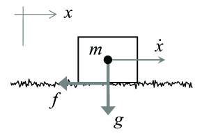
(a)           (b)

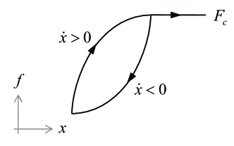
Figure 1. Schematic representation of kinetic friction (a), pre-sliding friction transitions in force-displacement plane (b).

The latter is opposed to direction of the relative displacement, indicated by the velocity $\dot{x}$, and is usually proportional to a normal load $g$ (caused by a point-mass $m$ as in the picture). Despite the hysteresis dissipation properties are well known and, so to say, typical for structural mechanics, see e.g. [12] and the references therein, and were largely covered also in the mathematical studies of hysteresis systems, see e.g. [11, 5], the hysteresis in frictional systems was also strongly accented in the system and control studies, see e.g. [2, 4].

Several empirical and phenomenological dynamic models of kinetic friction are known, most of which capture the hysteresis during pre-sliding in often different ways. Due to the use of nonlinear differential equations and often distributed parameters and dynamic states with switching, a rigorous analysis of the damping properties and state trajectories for such models has been and remains a non-trivial task. For instance, the hysteresis damping of LuGre and Maxwell-slip friction models were addressed in [14], while in [1] a generic approach of analyzing hysteretic friction was presented with use of the Masing rules, see e.g. in [5, 3] for details. In almost all frictional studies, an importance of extending the classical Coulomb friction law by the pre-sliding transitions was (at least on the edge) recognized. This comes, however, at the cost of significantly more complex dynamics of the overall system, for which even a simple one-parameter Coulomb friction law with discontinuity poses a significant challenge in finding the analytical solution for trajectories, cf. e.g. [15].

The Dahl model [7] was originally proposed for describing the transient behavior of the solid friction when it is piecewise elastic rather than viscous. It was probably a first attempt to circumvent the discontinuity in the classical Coulomb law of dry friction at the reversals. The Dahl model was widespread (also in industrial applications) for analyzing and simulating the solid friction occurring in the ball-bearing systems. Having only two tunable parameters, one of which is the Coulomb friction coefficient, the Dahl model in its simplified form appears suitable for a detailed analysis of hysteresis cycles and the associated energy dissipation.

This paper aims at investigating the dynamic behavior of a standard lumped-mass motion system subject to the pre-sliding frictional damping. Being motivated by the previous studies [4], [1], our goal is to provide a clear and straightforward relationship between the energy balance of reversals and state trajectories during the hysteresis cycles. The underlying motivation is to have a generic methodology that can be used for different modeling approaches when describing the rate-independent friction-force-displacement characteristics. Having said that, the following materials present the main results organized in two sections. In section 2, we discuss the unforced pre-sliding hysteresis oscillator, while establishing the energy balance and proving the convergence of hysteresis dissipation cycles. In section 3, we apply the developed analysis and exemplify the associated calculus by using the Dahl friction model. The conclusions are given in section 4.

2. Unforced pre-sliding hysteresis oscillator

The unforced motion dynamics within a pre-sliding frictional range, i.e. in some neighborhood to the motion reversals characterized by $\mathrm{sign}\left[\dot{x}(t^{+})\right]\neq\mathrm{sign}\left[\dot{x}(t)\right]$ and $-1<f(t)/F_{c}<1$, where $\dot{x}(t^{+})$ denotes the (limit) value of $x$ just after changing stepwise the sign i.e. when the time argument approaches $t$ from the right, can be described in the generic form as

(2.1) $$m\frac{d^{2}x}{dt^{2}}+f[x]=0,\quad\frac{dx}{dt}(0)\neq 0.$$

Here the inertial motion of the point mass $m$ is counteracted by the nonlinear restoring force $f[\cdot]$ which includes the frictional damping. Note that the counteracting friction force $f$ is written as function of the relative displacement $x$, since it is modeling an irreversible process which depends on $x(t)$ and its previous values, in particular after each motion reversal, i.e. when $\mathrm{sign}\left[\dot{x}(t)\right]$ changes. Further we stress that an unforced system response owing to nonzero initial conditions, cf. (2.1), is in focus of our discussion. The forced pre-sliding hysteresis oscillations, for which the right-hand side of (2.1) should otherwise contain a known exogenous value $u(t)$ in the sense of an applied external force, could extend the analysis presented here. However, it would go beyond the scope of this work.

In the following, for the sake of brevity, we will use the notation $\dot{o}$ for describing time derivative of $o$ with respect to time $t$; correspondingly the double dot above a variable, i.e. $\ddot{o}$, denotes the second-order derivative with respect to time, etc. Rewriting (2.1) with $\ddot{x}=\dot{x}d\dot{x}(dx)^{-1}$ and integrating subsequently both sides of the resulted equation yields

(2.2) $$m\int\dot{x}d\dot{x}=-\int f[x]dx.$$

Note that (2.2) is valid only in time intervals where $x(t)$ is monotone, that is assumed to be the case between any two consecutive reversal points. This leads to the energy balance of an unforced pre-sliding hysteresis oscillator, as the total kinetic and potential plus dissipated energies are written as

(2.3) $$\frac{1}{2}m\,\dot{x}^{2}+\int\limits_{x_{j}}^{x_{j+1}}f[x]dx=0,$$

for two successive reversal points $x_{j}\neq x_{j+1}$ at times $t_{j}<t_{j+1}$. Let us denote the first kinetic energy term in the above equation by $E_{k}$, and the second energy term associated with the restoring force by $E_{f}$. Depending on the restoring force $f$, that is generally nonlinear and history-dependent, the energy $E_{f}=E_{p}+E_{d}$ includes both, the potential energy $E_{p}(x)$ and the dissipation energy $E_{d}(C)$ along a path $C$. Since for each reversion instant $t_{i}$, where $i\in\mathbb{Z}^{+}$, the $\dot{x}(t_{i})=0$ is valid, one can analyze the energy balance of the reversal cycles by using the $E_{f}$ energies only, i.e. setting $E_{k}$ to zero. Note that several constitutive friction models with hysteresis (like the Dahl model assumed in the following) does not have the structure which would allow considering a dissipation rate $D\geq 0$ and, thus, following the principles of thermodynamics. Therefore, a meaningful energy balance can be evaluated only at the reversal points. Following to that, one can show that the total energy dissipated during one closed cycle $C=(x_{i},x_{i+1},x_{i+2})$, where the first and last reversion points coincide with each other i.e. $x_{i}=x_{i+2}$, is given by

(2.4) $$E_{d}(C)=\oint\limits_{C}f[x]dx=E_{f}(x_{i},x_{i+1})-E_{p}(x_{i})-E_{f}(x_{i+1},x_{i+2})+E_{p}(x_{i+2}).$$

Given $E_{p}(x_{i+2})=E_{p}(x_{i})$ for a closed path $C$ of one reversion cycle, the total net dissipated energy can be calculated as

(2.5) $$E_{d}=\int\limits_{x_{i}}^{x_{i+1}}f[x]dx+\int\limits_{x_{i+1}}^{x_{i}}f[x]dx.$$

First, let us briefly sketch the situation where the restoring force would map a piecewise linear spring, i.e. $f\equiv\bar{f}(x)=k\,x(t)$ on the interval $-1<f(t)/F_{c}<1$, with some positive stiffness coefficient $0<k<\infty$. Obviously, the energy due to the restoring force will have only the potential term, according to the Hooke’s law, and is then expressed by $E_{p}=0.5\,kx^{2}$. In this case, substituting $\bar{f}(x)$ into (2.5) and evaluating the definite integral yield

(2.6) $$\bar{E}_{d}=\int\limits_{x_{i}}^{x_{i+1}}kx\,dx+\int\limits_{x_{i+1}}^{x_{i}}kx\,dx=\frac{1}{2}kx^{2}\Bigr{|}_{x_{i}}^{x_{i+1}}-\frac{1}{2}kx^{2}\Bigr{|}_{x_{i}}^{x_{i+1}}=0.$$

The obtained result is intuitively logical since the linear restoring force is purely conservative and does not dissipate (or generate) any energy on the closed displacement cycles. This situation is illustrated in the $(x,f)$ plane in Figure 2 by the grey dot line. Note that once $|f(t)/F_{c}|\geq 1$, the $f$-force saturates at $\pm F_{c}$ level and, afterwards, behaves as a constant Coulomb friction term. Recall that such piecewise affine behavior can be well described by the Prandtl-Ishlinskii stop-type operator [11], as shown and discussed in [16] in the context of the Coulomb friction.

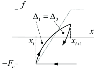
Figure 2. Energy balanced reversion points in $(x,f)$ plane.

Now, assuming the restoring force is a nonlinear map with memory, i.e. $f\equiv\hat{f}[x]\vee\check{f}[x]$ on the interval $-1<f(t)/F_{c}<1$, where $\hat{f}$ is an ascending branch for $\mathrm{sign}[\dot{x}]>0$ and $\check{f}$ is a descending branch for $\mathrm{sign}[\dot{x}]<0$, one can equally use (2.5) for calculating the net dissipated energy at one closed reversion cycle. More specifically, we assume $f[x]$ to be a clockwise rate-independent hysteresis, see e.g. in [5, 3] for basics on the hysteresis operators. Under this assumption, one can show the dissipated energy

(2.7) $$\tilde{E}_{d}=\int\limits_{x_{i}}^{x_{i+1}}\Bigl{(}\hat{f}[x]-\check{f}[x]\Bigr{)}\,dx=\Delta\neq 0.$$

This follows from the fact that for a clockwise hysteresis map, an ascending branch (in the time interval $t\in[t_{i},t_{i+1}]$) lies always above the descending branch (in the time interval $t\in[t_{i+1},t_{i+2}]$), given a pair of the input reversion points $x_{i}<x_{i+1}$. Such situation is shown in Figure 2 by the black solid line. The corresponding to (2.7) nonzero path integral

$$\oint\limits_{C}f[x]dx=\Delta$$

postulates the energy losses at one closed reversion cycle, i.e. $E_{d}(C)=\Delta$, which is equal to the area enclosed by a force-displacement loop, cf. Figure 1 (b). We will denote it by hysteretic energy dissipation and recall that, in general, the amount of energy dissipated during a cycle is proportional to the area of the enclosed hysteresis loop [5]. Important to notice is that the corresponding damping of an oscillatory system is rate-independent, similar to structural hysteresis damping that is common in material science and structural mechanics. It is also worth emphasizing that $\Delta\rightarrow 0$ if $\bigl{(}\hat{f}[x_{a}]-\check{f}[x_{b}]\bigr{)}\rightarrow 0$ for all $x_{a}=x_{b}$ on the intervals $x_{i}<x_{a}<x_{i+1}$ and $x_{i+1}<x_{b}<x_{i+2}$ of a closed cycle $C$. That means, it is the clockwise branching and formation of hysteresis loops that make the restoring term $f[x]$ dissipative in (2.1). Otherwise, a continuously increasing nonlinear but memory-free restoring force function $f(x)$ would lead to zero energy dissipation on the closed reversal cycles.

Now, we are in the position to address energy dissipation and decaying hysteresis cycles from a viewpoint of the balance equation (2.3) obtained for the system (2.1). Note that in the following, for the sake of simplicity and without loss of generality, we will consider the unity mass, meaning $m=1$.

Changing the variables of integration for the restoring force energy, cf. (2.3), one can rewrite it as

(2.8) $$E_{f}=\int\limits_{x_{i}}^{x_{i+1}}f[x]dx=\int\limits_{t_{i}}^{t_{i+1}}f[x]\,\dot{x}\,dt.$$

We consider an arbitrary pair of reversion points $x_{i}$ and $x_{i+1}$ as shown in Figure 2. Here the initial condition for the system (2.1) is $\dot{x}(0)<0$; this is without loss of generality. One can recognize that on the interval $\left[x_{i},x_{0}\right)$, where $x_{0}$ is the point of $f(x_{0})=0$, the integrand $f[\cdot]\,\dot{x}<0$, since $\mathrm{sign}(f)\neq\mathrm{sign}(\dot{x})$. On the opposite, the integrand $f[\cdot]\,\dot{x}>0$ on the interval $\left(x_{0},x_{i+1}\right]$, owing to the relative velocity and the restoring force have the same sign. That is after an initial reversal and until zero-crossing of the restoring force, the restoring power is first negative, which implies the energy of restoring force is converted into the kinetic one, cf. with (2.3). As a consequence, the system (2.1) accelerates and reaches the peak relative velocity $\dot{x}_{m}(t_{0})$ at time $t_{0}$ of the force zero-crossing. The peak relative velocity $|\dot{x}_{m}|=\max|\dot{x}(t)|$ is the maximal or minimal (depending on direction of the last reversal) on the interval $t_{i}\leq t\leq t_{i+1}$. Subsequently, after force zero-crossing, the restoring power becomes positive during $t\in\left(t_{0},t_{i+1}\right]$, meaning the kinetic energy $E_{k}$ is continuously converted into $E_{f}$ until reaching the next reversal with $\dot{x}(t_{i+1})=0$. Since both reversion points $x_{i}$ and $x_{i+1}$ are energetically balanced, cf. (2.3), one can see that the corresponding integral values have the same amount, i.e.

(2.9) $$\int\limits_{t_{i}}^{t_{0}}f[x]\,\dot{x}\,dt+\int\limits_{t_{0}}^{t_{i+1}}f[x]\,\dot{x}\,dt=0$$

also meaning the equal areas $\Delta_{1}=\Delta_{2}$, cf. Figure 2.

Now, let us demonstrate the convergence of such reversion cycles for the system (2.1), provided $f[\cdot]$ is a clockwise hysteresis map. Important to emphasize is that the first integral in (2.9) constitutes the potential energy which is transferred into the kinetic one until $t=t_{0}$. In contrast, the second integral in (2.9) is the superposition of the potential and dissipation energies, which are transferred from the kinetic energy until the next reversal at $t=t_{i+1}$. The potential energy part is the recoverable one when a new reversal occurs. Since the potential energy has its maximum value at the point of reversion, and the dissipation energy occurs on a way between two consecutive reversion points, one can state

(2.10) $$E_{p}(i)=E_{d}(i)+E_{p}(i+1).$$

Here we are using the argument $i\in\mathbb{Z}^{+}$ for labeling the reversion points. Realizing $E_{d}(i)\neq 0$ for all possible hysteresis branches leads to a recursion expansion

$$E_{p}(i)=E_{d}(i)+\underset{E_{p}(i+1)}{\underbrace{\Bigl{(}E_{d}(i+1)+E_{p}(i+2)\Bigr{)}}}=E_{d}(i)+\Bigl{(}E_{d}(i+1)+\bigl{(}\ldots\underset{E_{p}(i+n)}{\underbrace{(\ldots)}}\bigr{)}\Bigr{)},$$

with $n\rightarrow\infty$. It means that after each reversal, the amount of potential energy (cf. $\Delta$-areas in Figure 2) which can be then converted into kinetic one and thus drives the oscillator trajectories becomes smaller and smaller. At the same time, the total amount of the dissipated energy increases. This leads to the series expansion

(2.11) $$E_{p}(i)=\sum\limits_{n=i}^{\infty}E_{d}(n),$$

which converges to the potential energy of the initial reversion point, i.e. $E_{p}(i)$. Note that the initial potential energy is bounded from above by

(2.12) $$E_{p}(i)<\frac{1}{2\,k_{\min}}\,F_{c}^{2},$$

where $k_{\min}$ is the minimal possible equivalent stiffness of the restoring force $f[\cdot]$, cf. with the case exemplified by (2.6). This implies that the damped hysteresis oscillations of the system (2.1) are always amplitude bounded in the $(x,\dot{x})$ coordinates. At the same time, the damping rate an hence the state convergence, i.e. $\|(x,\dot{x})\|\rightarrow 0$, depend strongly on the analytic form of the hysteresis map $f[\cdot]$.

In the following, we apply the above developments to discuss in details the pre-sliding oscillations based on one possible modeling approach of capturing the Coulomb friction with continuous pre-sliding transitions, namely the Dahl model [8].

3. Application with Dahl model

The original Dahl model in the differential form is given by, cf. [8],

(3.1) $$\frac{dF(x)}{dx}=\sigma\Bigl{|}1-\frac{F}{F_{c}}\mathrm{sgn}(\dot{x})\Bigr{|}^{\gamma}\mathrm{sgn}\Bigl{(}1-\frac{F}{F_{c}}\mathrm{sgn}(\dot{x})\Bigr{)},$$

where $\mathrm{sgn}(\dot{x})$ captures the direction of relative displacement, i.e. the sign of velocity. The rest stiffness $0<\sigma\sim(dF/dx)$ when $|F|\ll F_{c}$, cf. [4], is a characteristic property of asperities of the contact surface. The shaping factor $\gamma\geq 0$ permits modulation of the form of displacement-force curves upon the reversion points. Worth mentioning is that for $\gamma=0$, the expression (3.1) becomes equivalent to the Prandtl-Ishlinskii stop-type operator with piecewise linear displacement-force transitions, cf. with [16] and example given around eq. (2.6). Also, if allowing for $\sigma\rightarrow\infty$ with $\gamma=0$, the Dahl model (3.1) will reduce to the classical Coulomb one, that has discontinuity at motion reversals, i.e. $F=F_{c}\mathrm{sgn}(\dot{x})$. Since $|F(t)|\leq F_{c}$ for all times $0\leq t<\infty$ it was proven in [4] that (3.1) can be written in a simpler form

(3.2) $$\frac{dF(x)}{dx}=\sigma\Bigl{(}1-\frac{F}{F_{c}}\mathrm{sgn}(\dot{x})\Bigr{)}^{\gamma}.$$

Also recall that for ductile type materials $\gamma\geq 1$, cf. [8]. In the sequel, we will assume $\gamma=1$ to keep our analysis with the associated integral calculus simpler and well tractable. It is also noteworthy that (3.2) with $\gamma=1$ is the most commonly used realization of the Dahl model, widely used for systems and control studies.

With the assumptions made above, we can rewrite (3.2) and obtain

(3.3) $$F_{c}\sigma^{-1}\,\frac{dF(x)}{dx}+F(x)\,\mathrm{sgn}(\dot{x})=F_{c}.$$

The above expression reveals several interesting observations about the Dahl model behavior. Namely, (i) the frictional force $F(x)$ monotonically approaches the Coulomb friction level since $|F|\rightarrow F_{c}$ after reversals, i.e. once the sign of $\dot{x}$ changes. (ii) this transient behavior does not depend on the time $t$ but on $x$ and, thus, represents a rate-independent $F(x)$ map. (iii) the transition mapping $F(x)$ does not explicitly depend on the coordinate of $x$ and is invariant to the location or translation of the reversion points $x_{i}$, cf. section 2. (iv) the convergence shape of $|F(x)|\rightarrow F_{c}$ depends on the ratio $\sigma/F_{c}$ between both frictional parameters of the system.

Solving (3.3), with the initial condition $F_{i}(x_{i})$ which corresponds to the last reversion point $x_{i}$, one obtains the restoring force $f[\cdot]\equiv F\bigl{(}x,F_{i}(x_{i})\bigr{)}$, cf. section 2, that represents locally the Dahl model written in the algebraic form

(3.4) $$f[x]=\mathrm{sgn}(\dot{x})\Bigl{(}F_{c}-\bigl{(}F_{c}-\mathrm{sgn}(\dot{x})F_{i}\bigr{)}\exp\bigl{(}-\mathrm{sgn}(\dot{x})\sigma F_{c}^{-1}(x-x_{i})\bigr{)}\Bigr{)}.$$

Since (3.4) captures bidirectional progress of the force-displacement curves, depending on $\mathrm{sgn}(\dot{x})$, hereinafter we will consider the positive sign of velocity, analogous to the situation shown in Figure 2 and without loss of generality. Hence, obtaining

(3.5) $$f_{+}[x]=F_{c}-\bigl{(}F_{c}-F_{i}\bigr{)}\exp\Bigl{(}-\frac{\sigma}{F_{c}}(x-x_{i})\Bigr{)}$$

and first solving $f_{+}[x]=0$ with respect to $x$, one can determine

(3.6) $$x_{0,i}=x_{i}-\frac{F_{c}}{\sigma}\,\ln\Bigl{(}\frac{F_{c}}{F_{c}-F_{i}}\Bigr{)},$$

which is the zero-crossing point of the restoring force, provided $F_{i}<0$, cf. with section 2 and Figure 2.

Now, in order to analyze energy produced by the restoring force we evaluate the antiderivative of (3.5), this with respect to the initial conditions, and obtain

(3.7) $$E_{f+}(x)=\int f_{+}[x]\,dx=F_{c}\,x+\frac{F_{c}^{2}}{\sigma}\exp\Bigl{(}-\frac{\sigma}{F_{c}}\,x\Bigr{)}-\frac{F_{c}^{2}}{\sigma}.$$

Worth noting is that the above result is consistent with analysis of the energy stored by the hysteresis loops of the Dahl model provided in [4]. Recalling that $E_{f+}(x)$ is defined only on the interval between two consecutive reversion points, i.e. $x\in[x_{i},x_{i+1}]$, and using the fact of the balanced energy due to restoring force, cf. (2.9) and Figure 2, one needs to consider (3.7) before and after zero-crossing point $x_{0}$. In addition, for the correct sign of the integrands in the energy balance (2.9) and, thus, for taking into account the initial conditions of integration (3.7), one has to assign $x_{i}$ in relation to $x_{0,i}=0$. Out from (3.6), one obtains

(3.8) $$x_{i}=\frac{F_{c}}{\sigma}\ln\Bigl{(}\frac{F_{c}}{F_{c}-F_{i}}\Bigr{)}<0,$$

which satisfies $-F_{c}\leq F_{i}<0$. When evaluating the definite integral of (3.5), with the set lower limit $x_{0}$ and upper limit $x_{i}$, one obtains the potential energy as a function of the restoring force at the reversion point:

(3.9) $$E_{p}(F_{i})=\frac{F_{c}^{2}}{\sigma}\Biggl{(}\ln\Bigl{(}\frac{F_{c}}{F_{c}-F_{i}}\Bigr{)}-\frac{F_{i}}{F_{c}}\Biggr{)}.$$

Note that (3.9) is also equal to the maximal kinetic energy over the interval $[t_{i},t_{i+1}]$, i.e. during the motion between the reversal points $x_{i}$ and $x_{i+1}$. Further we note that the potential energy is bounded from above, cf. with (2.12), by

$$\max E_{p}=0.3069\,\frac{F_{c}^{2}}{\sigma}$$

since $F_{i}\in[-F_{c},F_{c}]$. The potential energy (3.9) is visualized (on the logarithmic scale) in Figure 3 as a function of the normalized restoring force $|F_{i}|/F_{c}$. The curves are shown for the unitless ratio between the rest stiffness and Coulomb friction bound of the Dahl model, i.e. $\sigma/F_{c}=\{1,10,100,1000\}$.

Figure 3. Potential energy $E_{p}$ (on logarithmic scale) as a function of the normalized restoring force $|F_{i}|/F_{c}$ at the reversion point $x_{i}$.

One can recognize a considerable drop in the potential energy, closer to zero is the reversal state in terms of the restoring force. This serves also as an indication of how the potential energy and the corresponding hysteresis oscillations will decrease over the course of reversal cycles.

Once the potential energy (3.9) is known, with respect to the last reversal in $x_{i}$, we are interested to evaluate the restoring force energy which is balanced by the kinetic energy $E_{k}(t)=0.5m\dot{x}^{2}$. Recall that the kinetic energy is first continuously increasing until reaching its maximum value, i.e. with $\max|\dot{x}|$ at $t_{0}$, cf. section 2, and then continuously decreasing until zero velocity, that gives rise to the next reversal in $x_{i+1}$. This is reflected in the energy balance of the restoring force, implying $E_{f}(x_{i+1})=E_{k}(t_{0})=E_{p}(F_{i})$. One can recognize that in order to determine $x_{i+1}$ from (3.7), one needs to solve

(3.10) $$\frac{F_{c}^{2}}{\sigma}\,\Omega(x)+F_{c}x-\frac{F_{c}^{2}}{\sigma}=E_{f+}(x_{i})\quad\hbox{ with }\quad\Omega(x)=\exp\Bigl{(}-\frac{\sigma}{F_{c}}x\Bigr{)}$$

with respect to $x$. The above equation has the unknown variable $x$ both outside and inside the exponential function $\Omega$ and, thus, cannot be solved explicitly. Recall that a non-explicit solution of (3.10) would require the multivalued Lambert W-function, see e.g. [6] for details. Due to multivaluedness with complex numbers the Lambert W-function can hardly serve us to find the unique $x_{i+1}\in\mathbb{R}^{+}$. Instead, we are deriving a suitable linear approximation $\Omega^{*}$ which is sufficiently close to $\Omega$ on the interval $x\in[0,x_{i+1}]$. This should also take into account the parametric ratio $\sigma/F_{c}$ and the last reversal state, which is mapped through $F_{i}$ and affects the energy $E_{p}$, cf. (3.9). Requiring $\Omega(0)=\Omega^{*}(0)=1$ and $\Omega(x_{i+1})=\Omega^{*}(x_{i+1})$, the linearizing the exponential function in terms of $d\Omega/dx$, and afterwards analyzing the relationship to the last reversion point (3.8), we suggest

(3.11) $$\Omega^{*}(x)=1-\frac{\sigma}{F_{c}}\exp\Bigl{(}0.6\ln\Bigl{(}\frac{F_{c}}{F_{c}-F_{i}}\Bigr{)}\Bigr{)}\,x=1-K\bigl{(}\sigma,F_{c},F_{i}\bigr{)}\,x.$$

The exponential term $\Omega$ and its linear approximation $\Omega^{*}$ are shown in Figure 4, for different parameter ratios $\sigma/F_{c}^{(a,b,c)}=\{1,2,8\}$. Note that the different $\Omega^{*}$-slopes, each one touching the same exponential curve $\Omega^{(a,b,c)}$, correspond to different initial states $F_{i}=-F_{c}\times\{0.2,0.4,\ldots,1\}$.

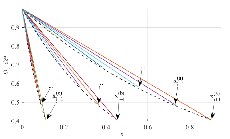
Figure 4. Exponential term $\Omega$ (black dash lines) and its linear approximation $\Omega^{*}$ (colored solid lines) for different parameter ratios $\sigma/F_{c}^{(a,b,c)}=\{1,2,8\}$ and initial states $F_{i}=-F_{c}\times\{0.2,0.4,\ldots,1\}$.

Since the $\Omega(x)$ term is reproduced sufficiently accurately by $\Omega^{*}(x)$, and that for each following inversion state $x_{i+1}$, we substitute (3.11) into (3.10) instead of $\Omega$, making it explicitly solvable. Following to that and solving

(3.12) $$\frac{F_{c}^{2}}{\sigma}\Bigl{(}1-K\bigl{(}\sigma,F_{c},F_{i}\bigr{)}\,x\Bigr{)}+F_{c}x-\frac{F_{c}^{2}}{\sigma}=E_{f+}(x_{i})=E_{p}(F_{i})$$

with respect to the unknown $x$, one can calculate

(3.13) $$x_{i+1}(F_{i})=\frac{E_{p}(F_{i})}{F_{c}}\,\Biggl{(}1-\frac{F_{c}}{\sigma}\Bigl{(}\frac{F_{c}}{F_{c}-F_{i}}\Bigr{)}^{3/5}\Biggr{)}^{-1},$$

where $E_{p}(F_{i})$ is determined by (3.9). With this intermediate result, one can directly evaluate the recovered potential energy in the next reversion point, i.e. $E_{p}(i+1)$, i.e. using (3.7) with integration limits $x_{0}$ and (3.13). For visualizing the development of the next reversal, in terms of the corresponding $(x_{i+1},F_{i+1})$ state, the force-displacement curves between two reversion points $i$ and $i+1$ are depicted in Figure 5, for the various Coulomb friction coefficients $F_{c}=\{1,1.5,2\}$.

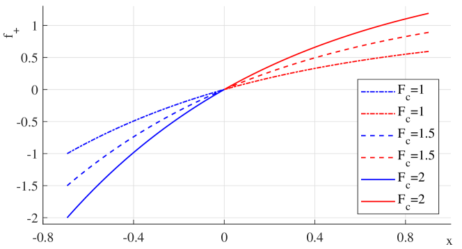
Figure 5. Force-displacement curves between two reversion points $i$ and $i+1$ for various Coulomb friction coefficients $F_{c}=\{1,1.5,2\}$.

One can recognize that even though $|x_{i+1}|>|x_{i}|$ here, which however depends on the $\sigma/F_{c}$ parametric ratio, the $|F_{i+1}/F_{i}|<1$ is always decreasing, thus resulting in an always valid relationship $E_{p}(i+1)<E_{p}(i)$.

Now, evaluating the potential energy at the following $(i+1)$-th reversal, i.e. computing $E_{p}(F_{i+1})$ for the next recursive step, cf. (2.10), we obtain

(3.14) $$E_{p}(i+1)=\frac{F_{c}^{2}}{\sigma}\Biggl{(}\ln\Bigl{(}\frac{F_{c}}{F_{c}-F_{i+1}}\Bigr{)}-\frac{F_{i+1}}{F_{c}}\Biggr{)}.$$

One can recognize that (3.14) allows for an explicit recursive form, so that it is always possible to compute $E_{p}(i+n)$ for all $i<n\leq\infty$ and the given initial state $(x_{i},F_{i})$. Recall that $E_{p}(i)-E_{p}(i+1)\equiv E_{d}(i)$, which is the dissipated energy between two consecutive reversals i.e. on one half of the hysteresis cycle. A decrease of potential energy $E_{p}(i)$ (on the logarithmic scale) between two consecutive reversals is shown in Figure 6, for different parametric ratios $\sigma/F_{c}=\{10,100,1000\}$.

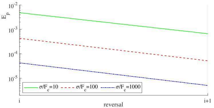
Figure 6. Potential energy $E_{p}(i+n)$ between two consecutive reversals, for different parametric ratios $\sigma/F_{c}=\{10,100,1000\}$.

One can recognize an exponential drop of $E_{p}(i)$ and, thus, an exponential rate of $E_{d}(i+1)$. Recall that the exponential rate of $E_{d}(i+1)$ and hence the convergence of the $x$ state is not in the time series but in the series of consecutive reversals of a decreasing hysteresis cycle. For a further growing number of reversals $n$, the energy dissipation and the corresponding convergence rate will result in a convergence slower than the exponential, as can be seen from Figure 7.

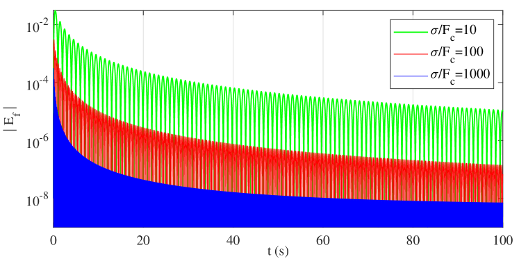
Figure 7. Time series of the energy magnitude from the numerical simulation of (2.1) with (3.4), for different parametric ratios $\sigma/F_{c}$.

Here, the total energy of restoring force $E_{f}$ is evaluated by the integrated power, cf. (2.8), when numerically simulating the time series of (2.1) with (3.4). The increasing frequency of the hysteresis cycles is visible for an increasing parametric ratio $\sigma/F_{c}$. One can also recognize that the envelope of the energy peak points, which are corresponding to the periodic reversals, has the same principal shape for all $\sigma/F_{c}$ ratios. Higher $\sigma/F_{c}$ ratios have an inverse biasing effect on the supposedly hyperexponential shape of convergence and provide a faster energy dissipation during some initial reversal cycles.

4. Conclusions

We considered the appearance of hysteresis cycles and the associated energy balance during the pre-sliding transients of kinetic friction. When an unforced second-order motion system has non-zero initial velocity, the structural hysteresis damping of contact surface asperities gives rise to largely decreasing nonlinear oscillations around zero equilibrium. Such behavior occurs alongside the so-called reversal cycles, where some restoring force energy is stored as potential energy but decreases with each successive reversal state. Supposedly, the associated energy dissipation and convergence of the state trajectories are neither exponential, i.e. viscous type, nor finite-time, i.e. Coulomb type.

We have analyzed such pre-sliding hysteresis cycles, being inspired by the pervious related works [4], [1]. We established an energy balance between the potential energy associated with each pair of two consecutive reversion states and the dissipated hysteretic energy during the half-cycle. In particular, we demonstrated a recursive series expansion of dissipated energies for an infinite sequence of reversion points and showed that this series converges to the upper bounded potential energy in the first (initial) reversal point. The analysis developed led to expressions for energies and force-displacement curves that allow application to various hysteresis models. The class of the suitable force-displacement mapping is limited to the rate-independent clockwise hysteresis functions.

As an illustrative example, we considered the Dahl model [7] of the solid Coulomb friction without discontinuities at the velocity zero-crossing. We developed an explicit approximation for the energies and states of the consecutive reversals, that allows analyzing the energy dissipation and state trajectories depending on the system parameters – the Coulomb friction coefficient and the so-called rest stiffness. This is also helpful for further convergence analysis and investigation of the motion stop in presence of Coulomb friction without discontinuity. Our analysis is in line with the original results demonstrated in [8], while providing an accurate estimation of the restoring force energy per half-cycle after each force zero-crossing, cf. with [8, Fig. 7]. The discussed energy dissipation by the Dahl model discloses further its main features and properties. Only asymptotic convergence of the motion state trajectories is possible with use of the Dahl model, cf. Figure 7. Thus, the corresponding kinetic energy tends towards zero with time towards infinity. This reveals some of the model’s weaknesses in relation to a more realistic and physically reasoned behavior of the pre-sliding kinetic friction.

The results of this study are applicable to other types of kinetic friction modeling with hysteresis and should contribute to a better understanding and prediction of the pre-sliding force-displacement properties, and the associated energy dissipation on the rubbing and slipping contact interfaces.

Authors’ addresses: Michael Ruderman, University of Agder, Kristiansand, Norway
e-mail: michael.ruderman@uia.no.

References

- [1] Farid Al-Bender, Wim Symens, Jan Swevers, and Hendrik Van Brussel, Theoretical analysis of the dynamic behavior of hysteresis elements in mechanical systems, International journal of non-linear mechanics 39 (2004), no. 10, 1721–1735.
- [2] Brian Armstrong-Hélouvry, Pierre Dupont, and Carlos Canudas De Wit, A survey of models, analysis tools and compensation methods for the control of machines with friction, Automatica 30 (1994), no. 7, 1083–1138.
- [3] Giorgio Bertotti and Isaak Mayergoyz, The science of hysteresis: 3-volume set, Elsevier, 2005.
- [4] Pierre-Alexandre Bliman, Mathematical study of the Dahl’s friction model, European journal of mechanics. A. Solids 11 (1992), no. 6, 835–848.
- [5] Martin Brokate and Juergen Sprekels, Hysteresis and phase transitions, Springer, Berlin, 1996.
- [6] Robert Corless, Gaston Gonnet, David Hare, David Jeffrey, and Donald Knuth, On the Lambert W function, Advances in Computational mathematics 5 (1996), no. 1, 329–359.
- [7] Philip Dahl, A solid friction model, Tech. report, Aerospace Corp El Segundo Ca, 1968.
- [8] by same author, Solid friction damping of mechanical vibrations, AIAA Journal 14 (1976), no. 12, 1675–1682.
- [9] James Greenwood, H Minshall, and David Tabor, Hysteresis losses in rolling and sliding friction, Proceedings of the Royal Society of London. Series A. Mathematical and Physical Sciences 259 (1961), no. 1299, 480–507.
- [10] Tadayoshi Koizumi and Hiroshi Shibazaki, A study of the relationships governing starting rolling friction, Wear 93 (1984), no. 3, 281–290.
- [11] Pavel Krejci, Hysteresis, convexity and dissipation in hyperbolic equations, Gattötoscho, Tokyo, 1996.
- [12] Walter Lacarbonara and Fabrizio Vestroni, Nonclassical responses of oscillators with hysteresis, Nonlinear Dynamics 32 (2003), no. 3, 235–258.
- [13] Vincent Lampaert, Farid Al-Bender, and Jan Swevers, Experimental characterization of dry friction at low velocities on a developed tribometer setup for macroscopic measurements, Tribology Letters 16 (2004), no. 1, 95–105.
- [14] Michael Ruderman, Presliding hysteresis damping of LuGre and Maxwell-slip friction models, Mechatronics 30 (2015), 225–230.
- [15] by same author, Stick-slip and convergence of feedback-controlled systems with Coulomb friction, Asian Journal of Control 24 (2022), no. 6, 2877–2887.
- [16] Michael Ruderman and Dmitrii Rachinskii, Use of Prandtl-Ishlinskii hysteresis operators for Coulomb friction modeling with presliding, Journal of Physics: Conference Series, vol. 811, 2017, p. 012013.