A global adaptive velocity space for general discrete velocity framework in predictions of rarefied and multi-scale flows
Abstract
The rarefied flow and multi-scale flow are crucial for the aerodynamic design of spacecraft, ultra-low orbital vehicles and plumes. By introducing a discrete velocity space, the Boltzmann method, such as the discrete velocity method and unified methods, can capture complex and non-equilibrium velocity distribution functions (VDFs) and describe flow behaviors exactly. However, the extremely steep slope and high concentration of the gas VDFs in a local particle velocity space make it very difficult for the Boltzmann method with structured velocity space to describe high speed flow. Therefore, the adaptive velocity space (AVS) is required for the Boltzmann solvers to be practical in complex rarefied flow and multi-scale flow. This paper makes two improvements to the AVS approach, which is then incorporated into a general discrete velocity framework, such as the unified gas-kinetic scheme. Firstly, a global velocity mesh is used to prevent the interpolation of the VDFs at the physical interface during the calculation of the microscopic fluxes, maintaining the program’s high level of parallelism. Secondly, rather than utilizing costly interpolation, the VDFs on a new velocity space were reconstruction using the “consanguinity” relationship. In other words, a split child node’s VDF is the same as its parent’s VDF, and a merged parent’s VDF is the average of its children’s VDFs. Additionally, the discrete deviation of the equilibrium distribution functions is employed to maintain the proposed method’s conservation. Moreover, an appropriate set of adaptive parameters is established to enhance the automation of the proposed method. Finally, a number of numerical tests are carried out to validate the proposed method, including supersonic flow around a circular cylinder in transitional regime, the cavity flow in continuum regime, supersonic flow around a blunt wedge in transitional regime, supersonic flow around sharp flat plate in slip regime, supersonic flow around truncated flat plate in slip regime and supersonic flow around sphere in slip regime and transitional regime.
keywords:
Multi-scale; Adaptive velocity space; Conservation; Adaptive parameters1 Introduction
For multi-scale flows, the physical scale varies over time and place. The Knudsen (Kn) number, which is defined as Kn = , is used to determine the degree of gas rarefaction, where is the mean free path of the gas, and is the characteristic length of the object in the flow. According to the Kn number, the flow can be qualitatively categorized into continuum flow regime (Kn 0.001), slip flow regime (0.001 Kn 0.1), transitional flow regime (0.1 Kn 10) and free molecular flow regime (Kn 10). Multi-scale flow is a term with a broad engineering background that refers to the coexistence of different flow regimes. For instance, considering the flow of near-space vehicles and micro-/nano-electro-mechanical systems (MEMS/NEMS), several flow regimes including continuum flow, slip flow, and even free molecule flow will exist in the same computational domain, and the local Kn number may fluctuate by many orders of magnitude. This multi-scale nature in both time and space makes the flows very difficult to be modeled and predicted.
In terms of flow numerical prediction, the traditional method of computational fluid dynamics based on Navier-Stokes (N-S) equations is suitable for continuum flows in the airspace and macro scale, whereas the model molecular method based on rarefied gas dynamics, represented by the direct simulation Monte Carlo (DSMC) [1] method, performs well for rarefied flows and micro-scale flows. However, each of the two methods has its difficulties in simulating multi-scale flow numerically [1, 2, 3]. Motivated by the N-S method’s and DSMC method’s successes in continuum flow and rarefied flow, researchers have combined the two methods through flow-field zoning to address the multi-scale flow problem, and the overlapping hybrid particle-continuum method is proposed [4, 5, 6]. The rarefied computing domain and the continuum computing domain must overlap to improve information transmission. To categorize the flow domain, empirical or semi-empirical criteria are typically used [7, 8]. The multi-scale problem can be partially resolved by the coupling approach, but it is still difficult to split the computational domain precisely and integrate several flow regimes reasonably [2].
In recent years, a class of multi-scale unified method, such as unified gas-kinetic scheme (UGKS) [9, 10], discrete unified gas-kinetic scheme (DUGKS) [11, 12], gas-kinetic unified algorithm (GKUA) [13, 14] and the improved discrete velocity method (IDVM) [15, 16], have been proposed, making it possible to solve complex multi-scale flows by using the same numerical method. With a local analytical integral solution of the kinetic model equation, the particle transport is coupled with particle collision processes in the UGKS, so that the time step and mesh size are independent of the collision time and the mean free path, respectively. The DUGKS is another multi-scale method based on the same physical process as the UGKS. Instead of the analytical integral solution, the characteristic difference solution of the kinetic model equation is adopted to reconstruct the multi-scale numerical flux at a cell interface. Therefore, the DUGKS can be regarded as a special version of UGKS. After a decade of development, many numerical techniques have been developed and implemented in the UGKS and DUGKS to increase the computational efficiency and reduce memory cost, such as unstructured mesh computation [3, 17], moving grids [18, 2], velocity space adaptation [2], memory reduction [19], wave–particle adaptation [20], implicit algorithms [21, 22, 23], parallelization algorithm [24], and further simplification and modification [25, 26, 27, 28]. With these improvement, the UGKS and DUGKS have been successfully applied to a variety of flow problems in different flow regimes, such as micro flows [29], compressible flows [12, 30], jet flow [2, 31], multi-phase flows [32], gas-solid flows [33], and gas mixture systems [34]. Besides flow problems, the UGKS and DUGKS were also extended to multi-scale transport problems such as radiative transfer [35], phonon heat transfer [36], plasma physics [37], neutron transport [38], granular flow [39], and turbulent flow [40, 41].
In the discrete velocity method (DVM) framework, a discrete velocity space is adopted to resolve the velocity distribution function (VDF), which contains detailed information about particle motion in a 6-dimensional phase space, for all points of physical space. Because of the wide spreading of the particle distribution in high-speed flows and the narrow-kernel particle distribution in cases with a large Kn number, the velocity space must have a local high resolution and cover a huge domain. The memory cost will be unbearable if a conventional structured velocity space is used [42]. The authors of [42, 22, 43] suggested to use a unstructured velocity space that is manually refined as necessary before numerical simulation. However, it could be challenging to generate an unstructured velocity space using as few elements as possible while still effectively capturing the flow behavior, especially for newcomers.
In recent years, the adaptive velocity space (AVS), which can automatically generate the corresponding velocity space according to the flow variables, has been proposed. Depending on whether the velocity space varies over time, the AVS technique can be divided into two groups, i.e. “fixed” and “unfixed”. An AVS was proposed by Aristov [44] for the simulation of the 1D shock structure. However, the technique has never been extended and is quite specific to this test case. Baranger et al. [45, 46] employ a compressible N-S pre-simulation result to locally refine the velocity mesh wherever it is necessary and to coarsen it elsewhere at the start of the numerical experiment. Then the velocity mesh is fixed until the end of the simulation. With the help of this technique, the amount of discrete velocity points can be significantly decreased. However, the accuracy of this “fixed” velocity mesh depends greatly on the N-S results, which are unreliable for rarefied and multi-scale flows. Chen et al. [2] and Arslanbekov et al. [47] proposed a “unfixed” local velocity mesh with a different velocity space for different time and space positions. An adaptive physical mesh is also used in Arslanbekov’s approach. Kolobov et al. [48] simultaneously developed a similar “unfixed” local AVS for plasma physics and rarefied gas dynamics. Bernard et al. [49] proposed a simple adaptation strategy that the local velocity mesh is only a sub-set of a global velocity mesh. And the domain of the velocity mesh is determined by the local temperature. However, these adaptive meshes are based on the same background velocity mesh, whose bound are fixed at the beginning of the computation and are constant in time and space. It is therefore attractive to allow for a dynamic adaptation of these bounds in time and space. Correctly estimating the borders can be difficult, but Brull and Mieussens [50] showed that it is achievable by using the conservation laws. This method was only proposed for one dimensional velocity variable so far.
The exchange of information between the velocity meshes of two adjacent physical cells is one of the challenges for local velocity mesh, and interpolation is necessary in the transport step to match the velocity points in the physical interface. This interpolation can lead to approximation errors and possible increasing computational time [49]. On the other hand, the interpolation of the VDFs between two adaptive velocity meshes during the particle-redistribution over different velocity level can also lead to approximation errors and possible increasing computational time, and the conservation of the solution must be carefully maintained. Additionally, the parallel computing of the local velocity mesh is also more challenging.
In this paper, an “unfixed” global AVS technique for the general DVM framework is proposed, which is interpolation-free and simple to implement. The global velocity mesh ensures that there is no interpolation required for the calculation of microscopic flux at the physical interface in the transport step. And excellent parallel performance of algorithm is maintained. Furthermore, a novel “consanguinity” relationship is employed to avoid the interpolation in the reconstruction of VDFs. Thanks to this “consanguinity” relationship, it is not necessary to know the geometric relationship between the velocity elements, which makes the data structure quite simple. Finally, the discrete deviation of the equilibrium distribution functions are employed to maintain the proposed method’s conservation.
The rest of the paper is organized as follows: The conservative implicit unified gas-kinetic scheme is introduced in section 2 along with a predicted equilibrium state and simplified multi-scale flux. The details of the global AVS technique are presented in section 3. In section 4, a series of numerical experiments are conducted to verify the proposed methods. The conclusion is the final section.
2 Conservative implicit unified gas-kinetic scheme
This section will provide a quick overview of the conservative implicit UGKS (IUGKS) [22].
2.1 Gas-kinetic models
The Boltzmann equation serves as the basis for the UGKS:
| (1) |
where is the VDFs for particles moving in D-dimensional physical space with a velocity of at position and time t. Here, is the dummy velocity (with the degree of freedom ) consisting of the remaining components of the translational velocity of particles in three-dimensional space; is a vector of elements representing the internal degree of freedom of molecules; is the collision operator. Many kinetic models, including the Bhatnagar-Gross-Krook (BGK) collision model [51], the Shakhov model [52], the ellipsoidal statistical model (ES model) [53], and the Rykov model [54], have been proposed and used in the research of rarefied flows to simplify the collisional model of the full Boltzmann equation. To build kinetic models and develop the corresponding gas-kinetic schemes, numerous attempts have been made. The modeling of monatomic gases only considers the non-equilibrium transitional energy. In addition to the three translational degrees of freedom for the diatomic molecule, there are internal degrees of freedom, i.e., two degrees of freedom for rotation at room temperature. The degrees of freedom associated with vibrations begin to arise at a temperature higher than 1000 K. Thus, only the degrees of freedom for translation and rotation are considered in this study, and the UGKS is established by using the Shakhov model for monatomic gas and the Rykov model for diatomic gas.
The following presents the expression for the control equation of the Boltzmann-BGK type:
| (2) |
where is the relaxation time for the translational degree of freedom and can be calculated as , where and are the viscosity and pressure determined by the translational temperature instead of the equilibrium temperature . The energy equalization theorem is satisfied by the equilibrium temperature , the translational temperature , and the rotation temperature . represents the Maxwell equilibrium VDFs, Shakhov equilibrium VDFs, or Rykov equilibrium VDFs. The variable hard sphere (VHS) model is adopted in this study to determine viscosity
| (3) |
where and are the density and the specific gas constant, respectively. The viscosity of the freestream flow is correlated with the gas mean free path in the following way:
| (4) |
where T is temperature.
In the non-dimensional system, the Kn number is defined as:
| (5) |
where Ma = and Re = are the Mach (Ma) number and Reynolds (Re) number, respectively, and is the specific heat ratio. is the characteristic length. According to the inter-molecular interaction model, is set to 0.5, 0.81 and 0.74 for the hard sphere model, ideal argon and nitrogen, respectively.
2.2 Reduced gas-kinetic models
The discrete velocity space should be used to record the free transit of molecules, which is dependent only on the D-dimensional particle velocity and is not related to and (for diatomic gas). The following reduced VDFs [55] are used in the current numerical scheme to prevent discretizing and :
| (6) | ||||
The physical meaning of , , and is the distribution of the mass, translational internal energy, and rotating energy in the dummy velocity space and rotational energy space, respectively. The quasi-linear feature of the model equation is advantageous for this condensed treatment. Only the simplified VDFs and are required for monatomic gases. The reduced VDF for rotational energy will also be introduced for diatomic gases. Note that will inevitably vanish in three dimensions. Then, the macroscopic variables can be expressed as:
| (7) |
where, is the total energy density, is the inertial energy density, and is the rotational energy density. The translational heat flux, rotational heat flux, and total heat flux are expressed as:
| (8) | ||||
where is the peculiar velocity.
The governing equation of the reduced VDF is:
| (9) | ||||
For simplicity, Eq. 9 can be rewritten as
| (10) |
where stands for , and .
For monatomic gas flow, the Shakhov equilibrium is:
| (11) | ||||
with
| (12) |
| (13) |
| (14) |
where the Prandtl (Pr) number equals 2/3, and represents the Maxwell equilibrium:
| (15) |
For diatomic gas flow, the Rykov equilibrium is:
| (16) | ||||
with
| (17) | ||||
| (18) | ||||
| (19) | ||||
where the coefficients are set as: , , and for nitrogen [10, 22] in this study. is the rotational relaxation collision number accounting for the ratio of the slower inelastic translation–rotation energy relaxation relative to the elastic translational relaxation.
All the above equilibrium VDFs can be obtained by macroscopic variables.
2.3 IUGKS with simplified multi-scale flux
2.3.1 Macroscopic implicit governing equations
The finite volume method is used in physical space, the implicit backward Euler method is used in time, and then the implicit discrete macroscopic governing equation can be written as:
| (20) |
where and denote the volume of and the time interval, respecitvly. denotes the neighboring cell of cell and is the set of all of the neighbors of . denotes the variable at the interface between cell and . is the interface area. The source term is expressed as
| (21) |
where is the rotational energy density at the thermal equilibrium state. Replace with the predicted , and rearrange Eq. 20 into the incremental form
| (22) |
where the symbol denotes the predicted variables for the next time level. The flux is determined
| (23) |
where the construction of (i.e. , and ) will be detailed in Section 2.3.3. The variation of the flux is approximated by
| (24) |
where has the form of the well-known Roe’s flux function
| (25) |
Here is the Euler flux
| (26) |
and is
| (27) |
where is the acoustic speed at the interface, is the external normal unit vector of interface, and is the distance between cell center and .
Substituting Eqs. 24 and 25 into Eq. 22, and noting that holds, then we can get the expression
| (28) | ||||
Note that the source terms of the conserved variables , and are zero, and the source term of rotational energy is handled as
| (29) |
Therefore, for , it has
| (30) | ||||
Eqs. 28 and 30 are solved by the Symmetric Gauss–Seidel (SGS) method, or also known as the Point Relaxation Symmetric Gauss–Seidel (PRSGS) method [56, 57].
2.3.1 Microscopic implicit governing equations
Since we have obtained the predicted macroscopic variable vector , it is the time to deal with the microscopic implicit discrete Eq. 16 for . Similarly, rearrange Eq. 16 into the incremental form
| (31) |
where and are determined by the predicted . will be detailed in Section 2.3.3. is simply handled by the upwind scheme and Eq. 31 is turned into
| (32) | ||||
where is the set of ’s neighboring cells satisfying while for it satisfies . Eq. 32 is solved by the SGS method to obtain .
More information about the IUGKS is provided in reference [22], which recommends 2 times’ SGS iterations for the microscopic equation and 60 times’ SGS iterations for the macroscopic equation per time step.
2.3.3 Simplified multi-scale numerical fluxes
In this study, the simplified multi-scale flux is built utilizing the numerical quadrature solution, following the lead of DUGKS. As seen in Fig. 1, the VDF at the interface can be obtained by integrating the kinetic Eq. 10 along its characteristic line from to
| (33) |
where denotes a half-time step, and denotes the midpoint of the interface. Finally, the VDF at the interface can be expressed as:
| (34) |
where can be derived from the macroscopic variables of the interface. Since the collision operator conserves mass, momentum, and energy, the conserved variables can be computed from
| (35) |
where is vector of the elementary collision invariants. And the rotational ernergy can be computed from
| (36) |
Fianlly, can be calculated through the Taylor expansion at the control volume:
| (37) |
where represents the control volume which is centered at point C (Fig. 1). If , point C is (the center of the left cell) in Fig. 1; otherwise, point C is (the center of the right cell). is the gradient of the reduced VDFs at point C, which is calculated by the least-square method in this study, and is the gradient limiter used to suppress the numerical oscillations. Besides, the Venkatakrishnan limiter [58] is chosen in this paper.
3 Detail of the global adaptive velocity space technique
It is necessary to employ an AVS to improve the computational efficiency of UGKS, particularly for hypersonic non-equilibrium flows. Similar to the unstructured velocity space, the AVS in this study also uses the mid-point quadrature formula. Therefore, the quadrature point (i.e. discrete velocity point) and the quadrature weight are the center and volume (area for 2-dimensions case) of the velocity mesh, respectively. Because of the usage of the global velocity mesh and the “consanguinity” relationship during the reconstruction of VDFs in a new velocity space, the AVS technique described in this paper does not require knowledge of the geometric relationship between the elements. As a result, the data structure is quite simple and the proposed method is highly practical.
3.1 Tree data structure for adaptive velocity space
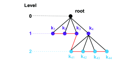
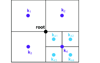
In this work, the quadtree and octree data structures are used to describe the two-dimensional (2D) and three-dimensional (3D) AVS, respectively. And the merging and splitting steps of the adaptation are illustrated using quadtree data for simplicity of description. In Fig. 2(a), the level of root node is 0, and it can only be split, not merged. The root node splits once would produce four child nodes () with level 1. Once the child node meets the split condition, it splits again and produce four child nodes () with level 2. The root node is the parent of nodes , while node k4 is the parent of nodes . The four child nodes that share the same parent node are brother nodes. Like a leaf on a tree, a node with no child is called leaf node. The leaf nodes in Fig. 2(a) are connected by a red lines and the corresponding velocity mesh is given in Fig. 2(b). As can be observed, the velocity mesh only has the leaf nodes , , , , , and . In addition, the leaf nodes are saved as double link lists in the computer code. The merging process, which can be regarded of as the inverse of the splitting process, can only take place when all four of the brother nodes are leaf nodes and the merging condition are satisfied. For instance, the child nodes can only be merged into the node if they all satisfy the merging condition. As a result of this merge step, the parent node becomes a leaf node and has no child.
3.2 Reconstruction of distribution functions
Following the adaptation of the velocity space, the VDF must be recreated on the new velocity space. In this study, the reconstruction of VDFs is done using a special “consanguinity” relationship rather than interpolation. Without losing generality, Fig. 2 is also used as an example to show the reconstruction of VDFs. For instance, the VDFs of nodes are equal to thier parent’s when the root node splits into four child nodes
| (38) |
where and are the VDF for the old velocity space before adaptation and the new velocity space after adaptation, respectively. The subscript is . Similarly, when node splits into four child nodes (), the VDFs of the child nodes are identical to that of node
| (39) |
For the merging step, the VDF of the merge node is equal to the average of the VDFs of its child nodes. For instance, the VDF of node can be calculated as the average of the VDFs of nodes when their four child nodes merge to thier parent node
| (40) |
Similar to this, when nodes merge to form root node, root node’s VDF is equal to the average of those nodes’ VDFs
| (41) |
Without a doubt, the ”consanguinity” relationship that has been proposed is quite simple and effective. Furthermore, since interpolation is not used, the velocity space data structure is not required, making the double link list fairly simple.
3.3 Conservation correction
The conservation of mass is met during the reconstruction of the VDFs in the preceding subsection, but it is not yet possible to guarantee that momentum and energy are also conserved. It is possible that some deviation exist in the VDFs obtained from the “consanguinity” relationship and need to be fixed to preserve conservation. The deviation physical variables can be computed from
| (42) |
where is the collision invariant. In line with the literature [22, 59], the discrete deviation of the equilibrium VDF is used to guarantee conservation. Consequently, the adaptive VDF can be described as
| (43) |
where is the macroscopic variables updated by Eq. 7 and is the Maxwellian VDF corresponding to .
For weakly nonequilibrium flows, the reconstruction of VDFs mentioned previously can also be bypassed, and the adaptive VDF can be represented as
| (44) |
3.4 Adaptive criterion
The AVS is significantly influenced by the adaptive criteria, which guide the merging and splitting process. In this work, the density criterion and the internal energy criterion, also known as the and criterion, respectively, are applied in line with literature [2]. Following are the definitions for and
| (45) |
| (46) |
where and are the element index of physical mesh and velocity mesh, respectively. is the area (2D) or volume (3D) of the -th velocity mesh element. We can infer from the definition of and that they stand for the density and internal energy ratios to the total density and internal energy at the current velocity element, respectively. The terms and refer to the density and internal energy ratios to the total density and internal energy at the present velocity element, respectively. Since a global velocity mesh is adopted, a maximum value from and in the whole physical mesh must be selected
| (47) |
Following is a description of the adaptive rules using and () as the splitting and merging thresholds, respectively
(a) When is larger than , the velocity mesh has to be split.
(b) When is smaller than , the velocity mesh speed needs to be merged.
(c) Besides (a) and (b), the velocity element does not need to be changed.
It is clear that is in charge of splitting, whereas is in charge of merging. When the contribution of density or interal energy of -th velocity element is large enough, i.e. , the -th velocity element is marked and are going to split. When the contribution of density or internal energy of -th velocity element is small enough, i.e. , the -th velocity element is marked and are going to merge.
3.5 Configuration of adaptive parameters
The potential to describe the behavior of flow depends on the domain and resolution of velocity space, which are controlled by adaptive parameters. Consequently, it is crucial to choose these adaptive parameters. A set of adaptive parameters are provided in this work to improve the automation of the AVS. Since the Maxwell distribution and the normal distribution are relatively similar, the characteristics of the normal distribution can be used to predict the distribution of the VDFs. The expression of the normal distribution is
| (48) |
where is the mean or expectation of the distribution, while and are the standard deviation and variance. When comparing Eq. 15 (Maxwell equilibrium distribution) with Eq. 48 (normal distribution), it is discovered that the expectation and standard deviation of Maxwell distribution are and , respectively. In numerical simulation, there are typically three standard deviation
| (49) |
where , and are static temperature (also known as the temperature of freestream), total temperature and wall temperature, respectively. And the total temperature is related to static temperature via
| (50) |
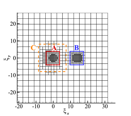
According to the features of the normal distribution, the probability of the and intervals with the expectation as the center is known to be 99.73 and 99.99, respectively, which can be viewed as 100. Therefore, the and are chosen as critical value for this work. Fig. 3 presents diagram of the AVS. The radius of the velocity domain is . The center of the velocity domain is rather than zero because there are three refined zones: the stationary zone (red A zone in Fig. 3), the freestream zone (blue A zone in Fig. 3) and the separated zone (orange C zone in Fig. 3). The radius and center of the stationary zone are and , respectively. The radius and center of the freestream zone are and , respectively. And the radius and center of the separated zone are and , respectively. The segregated zone is designed for the bottom of the vehicle’s separate flow. Most of the time, is enough because the wall temperature is significantly lower than the total temperature. However, the radius of the velocity domain should be larger, such as , to cover a larger stationary zone and separated zone when the wall temperature is close to the total temperature.
In general, the freestream zone has the highest resolution, followed by the stationary zone. Assuming that the velocity mesh’s standard interval is , the corresponding level of the mesh can be determined as
| (51) |
Consequently, the level of the freestream zone, or the maximum level of the AVS, is chosen as
| (52) |
And the interval of the freestream zone, or the minimum interval, is
| (53) |
It can be observed that is not larger than and not less than . In this work, is set as 0.6. Once the level of the freestream zone has been determined, the level of the stationary zone can be estimated as follows
| (54) |
And the following is the minimum level of the AVS
| (55) |
Additionally, the separated zone should be refined if there is a separated flow
| (56) |
where is the magnitude of the discrete velocity. Now that the geometric shape of the velocity space and the level scope have been presented, all that is left to do is choose the appropriate adaptive thresholds and .
When and , the normal distribution (Eq. 48) turns to the standard normal distribution
| (57) |
The maximum value of the standard normal distribution is found at , and the critical value is located where x equals to or . As was already discussed, the probability of the normal distribution falling inside the interval is around 100, hence the portion outside the interval can be neglected. With the help of this feature, the merging threshold is related to the splitting threshold via
| (58) |
where
| (59) |
Eq. 58 suggests that only when is less than will the velocity element be marked and begin to merge. Therefore, only the parameter needs to be determined, and the law of will be investigated in a later simulation of flow over a cylinder.
Once every adaptive parameter has been determined, an AVS can be created at step 0
(1) Create an element with just a root node, whose level is 0. The center and the radius of this element are and .
(2) Split the single element times results in a unified mesh of elements, where can be set to .
(3) Perform once adaption based on freestream point and static point, whose physical varibles are and . And the VDFs of and are equal to and . Therefore, can be computed according to Eqs. 45, 46 and 47.
As a result, an initial AVS is obtained. To efficiently match the flow field, adaptation is done in the first steps (like steps 1, 2, and 3). Following that, adaptation takes place at a frequency of . In general, can be set to 50 or 100 steps.
4 Numerical experiments
Several test cases are performed in this section to validate the proposed method, and the results of the AVS and the Cartesian velocity space (CVS) are compared to benchmark results.
4.1 Supersonic flow passing a circular cylinder
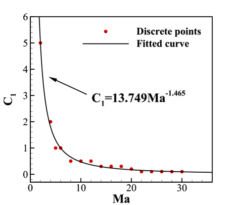
In this case, the relationship between and Mach number will be investigated. The Kn number of freestream with the cylinder radius as characteristic length is 1.0. The working gas is argon and the gas constant of argon is ). The VHS model with is employed. The specific heat ratio and the Prandtl number are 5/3 and 2/3, respectively. The temperature of the freestream and the surface of the cylinder both are 273 K. In this work, the characteristic length serves as the reference length, and the freestream’s density and temperature serve as the reference density and temperature. As a result, freestream’s dimensionless density and temperature are both equal to 1.0. The radius of the cylinder is 1.0 and the physical domain, which is a circular region with a circle center at (0,0) and a radius of 15, is discretized by a mesh with 64x61 cells. To accurately capture the heat flux on the cylinder surface, the height of the first mesh layer at the surface is 0.01 in this instance. Simulations were conducted in both CVS and AVS in order to compare the results. When Ma is 2 to 6, 8 to 20, and 22 to 30, the CVS with discrete points of , , and are used, respectively. The details of the AVS for supersonic flow passing a circular cylinder are presented in Table I. And a curve was fitted based on the discrete data in Table I to indicate the relationship between and Ma
| (60) |
The discrete data of Table I are plotted in Fig. 4, together with Eq. 60, making it clear that the parameter obtained from Eq. 60 is greater than zero. Consequently, the adaptive parameter will then be determined by Eq. 60.
| Ma | Element | ||
|---|---|---|---|
| 2 | 5.0 | 4 | 136 |
| 4 | 2.0 | 5 | 268 |
| 5 | 1.0 | 5 | 232 |
| 6 | 1.0 | 6 | 670 |
| 8 | 0.5 | 6 | 526 |
| 10 | 0.5 | 6 | 742 |
| 12 | 0.5 | 7 | 796 |
| 14 | 0.3 | 7 | 748 |
| 16 | 0.3 | 7 | 658 |
| 18 | 0.3 | 7 | 610 |
| 20 | 0.2 | 7 | 874 |
| 22 | 0.1 | 7 | 856 |
| 24 | 0.1 | 8 | 1348 |
| 26 | 0.1 | 8 | 1360 |
| 28 | 0.1 | 8 | 1270 |
| 30 | 0.1 | 8 | 1174 |
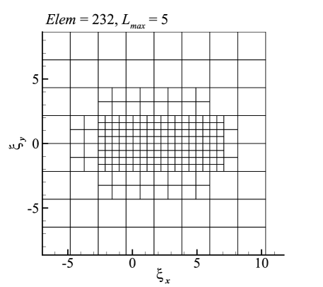
The results of Ma 5 supersonic flow around a cylinder in literature [3] will be employed as a benchmark. In literature [3], an CVS with the range of is adopted. According to Eq. 60, the parameter is 1.30, and Fig. 5 shows the corresponding AVS with a maximum level of 5 and 232 elements. There will be 1024 elements in the complete mesh of level 5, which is just 12.9 of the CVS’s elements and 4.4 times that of AVS. Furthermore, the elements of AVS is only 2.9 of the CVS’s.
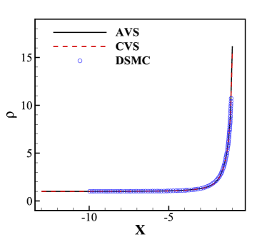
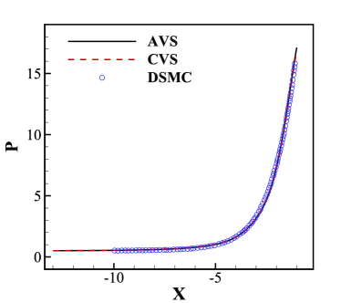
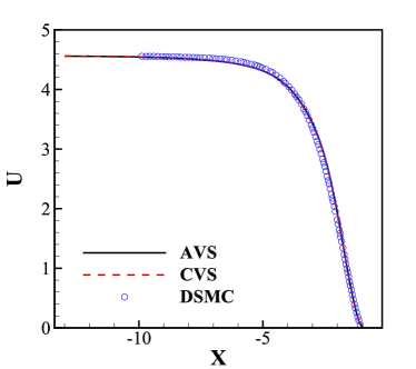
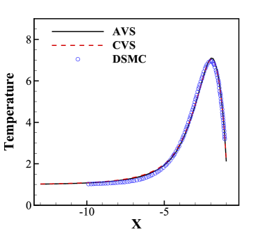
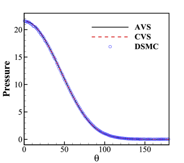
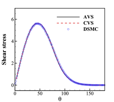
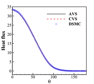
Fig. 6 presents the density, pressure, horizontal velocity (U) and temperature along the central line in front of the cylinder. Fig. 7 presents the pressure, shear stress and heat fluxes on the surface of cylinder. It is clear that the results from AVS, CVS and DSMC match one another. This indicates that the AVS can accurately describe the behavior of cylinder flow.
4.2 Lid-driven cavity flow
Although AVS is typically employed for high-speed non-equilibrium flows, it is interesting to find out if it is suitable for low-speed continuum flows. The test case of lid-driven cavity flow is very suitable to test whether the proposed method can accurately simulate the viscosity effect of the flow or not.
Here, the lid-driven cavity flow with Ma = 0.16 and Re = 400 and 1000 are carried out. The top wall is moving with a constant velocity while the other walls are static. The working gas is argon and the VHS molecular model is employed with . The temperature of all walls are 273 K, then the sonic speed and velocity of the moving wall are m/s and = 49.22 m/s, respectively.
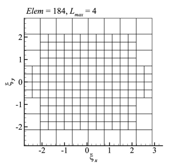
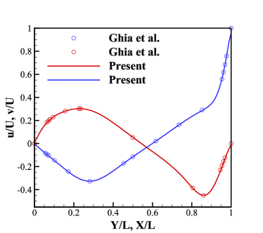
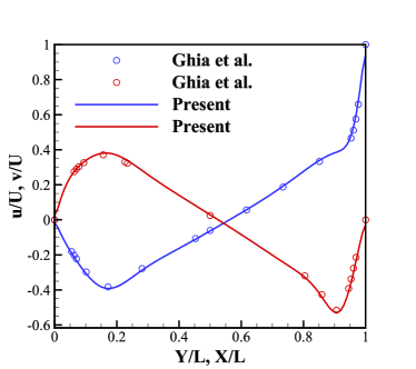
The physical domain is discretized by a uniform mesh with 100×100 cells, and the AVS with equals to 201.5 is shown in Fig. 8, which contains 184 elements. Fig. 9 presents the vertical velocity along the horizontal central line and the horizontal velocity along the vertical central line. The numerical results are in good agreement with the benchmark data [60]. It demonstrates that the AVS is capable of simulating low-speed continuum flows.
4.3 Hypersonic flow over a blunt wedge
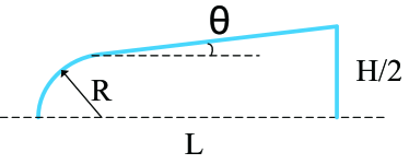
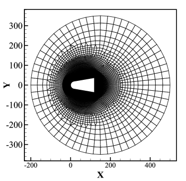
It is crucial to accurately predict the hypersonic bottom flow for near-space vehicles, particularly when Reaction Control System (RCS) is installed on the bottom of some vehicles. With reference to the configuration of the literature [61], the current method simulates the same issue to verify its performance for the hypersonic dilute expansion flow. Fig. 10 presents the geometry of the blunt wedge, which has a length of =120 mm, a head radius of =20 mm, a bottom height of =74.72 mm, and a body slope of =10°. Here, the working gas is argon and the VHS model is employed. The Ma number and angle of attack of freestream are 8.1 and 0°, respectively. The temperature of freestream is 189 K (equivalent to an altitude of 85 km), while the temperature of the surface of wedge is fixed at 273 K. The Kn number with and as the characteristic length are 0.338 and 0.090, respectively.
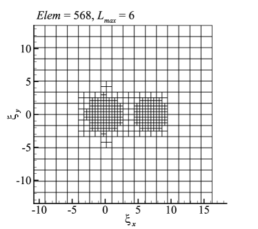
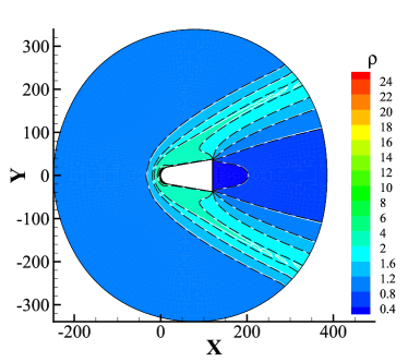
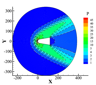
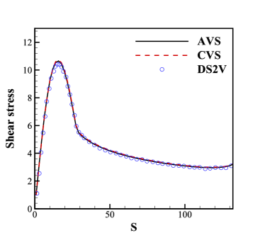
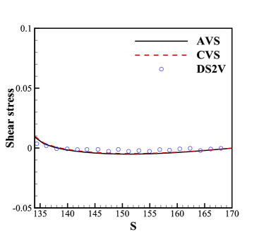
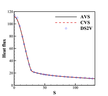
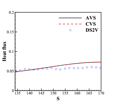
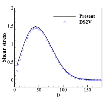
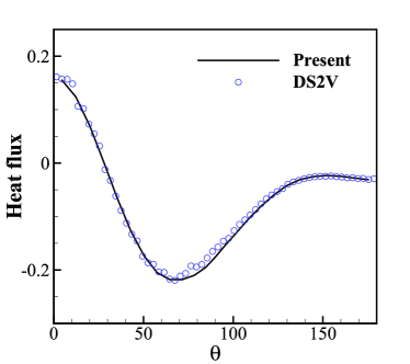
In this simulation, the unstructured physical mesh, which has 11905 cells, is shown in Fig. 11. The parameter according to Eq. 60 is 0.64, and the AVS, which include 568 elements, is shown in Fig. 12. In addition, the CAS with 7921 () elements was also adopted to simulate the flow around the blunt wedge. Figs. 13 present the density, pressure, temperature and horizontal velocity (U) contours around the blunt wedge. The background and white solid lines are the results of the CVS, whereas the black long dash line is the result of the AVS. It is obvious that the results of AVS and CVS are in good agreement with one another. The pressure, shear stress and heat flux along the surface of the blunt wedge are present in 14, 15 and 16, respectively. As can be observed, the results of AVS and CVS are consistent and in good agreement with those of DS2V.
4.4 Supersonic flow passing a sharp flat plate
To further verify the proposed approach, diatomic gas (i.e. nitrogen) will then be employed as working gas. Additionally, the computational efficiency of AVS will be investigated in the simulation of supersonic flow across a sharp flat plate.
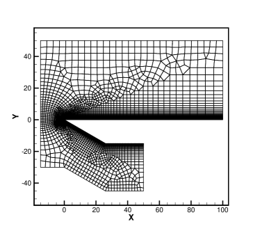
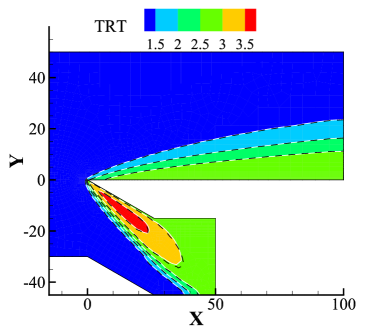
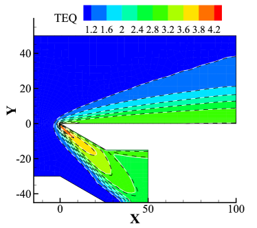
The configuration is the same with the run34 case in Ref. [62]. Fig. 17 presents the physical mesh used for calculation and the flat plate’s geometric shape. With a thickness of 15 mm and an upper surface length of 100 mm, the flat plate has a sharp angle of 30 degree. The Rykov model is employed with nitrogen serving as the working gas (). And the VHS molecular model is employed with . The surface temperature of the flat plate is fixed at 290 K, and the freestream’s Ma number and temperature are 4.89 and 116 K, respectively. The Kn number of freestream with the plate’s length as characteristic length is 0.0078.
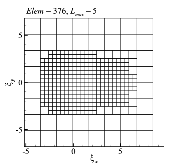
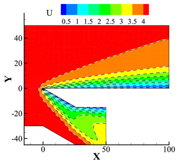
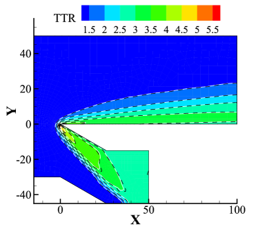
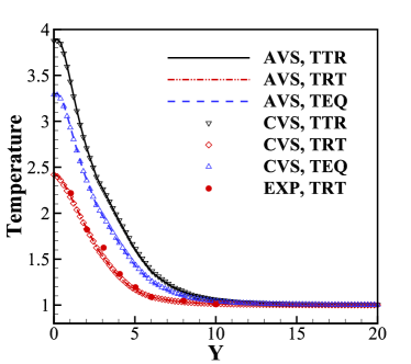
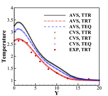
A uniform freestream flow is employed as the initial flow field in this simulation, and the splitting threshold is 1.34. The AVS is shown in Fig. 18. The AVS in Fig. 18 has only 376 elements, while the CVS of Reference [63] has 4800 elements. Fig. 19 presents the horizontal velocity, translational, rotational, and equilibrium temperature contours around the flat plate. The background and white solid lines are the results of the CVS, whereas the black long dash line is the result of the AVS. It is obvious that the results of AVS and CVS are in good agreement with one another. The temperature distributions along the vertical line above the flat plate at the locations of mm and mm from the leading edge are presented in Fig. 20. The numerical results match well with the experimental data. The AVS’s capability for capturing flow behavior around the flat plate is demonstrated by the strong agreement between the results from the AVS and the CVS.
The proposed AVS is more attractive since it has fewer elements than CVS, which lowers memory costs and speeds up computation. It should be noted that the sharp plate simulation had an adaptive frequency of and just one adaptation was done at step 0, indicating that the initial AVS at step 0 is suitable for this simulation. Table II shows the comparison of details between CVS and AVS for the sharp flat plate simulation, which were performed on 2 and 22 cores, respectively. Where “NC” in Table II means the number of elements per core. Using the results of 2 cores as a reference, the parallel efficiency for CVS and AVS are 77.90 and 45.56, respectively. It makes sense that when “NC” decreases, the proportion of calculation time to communication time decreases, resulting in a decrease of parallel efficiency. Anyway, compared to the CVS, the AVS costs much less time. The ratio of computation time for two cores is 12.06, which is nearly equal to the ratio of elements (12.77).
| - | CVS | AVS | Ratio |
|---|---|---|---|
| Elements | 4800 | 376 | 12.77 |
| NC of 2 cores1 | 2400 | 188 | 12.77 |
| NC of 22 cores1 | 218.18 | 17.09 | 12.77 |
| Computation time of 2 cores | 17942.95 | 2093.82 | 12.06 |
| Computation time of 22 cores | 1487.51 | 296.84 | 7.05 |
| Ratio of time (Speedup) | 8.57 | 5.01 | 1.71 |
| Ratio of core | 11 | 11 | 1 |
| Parallel efficiency | 77.90 | 45.56 | 1.71 |
-
1.
1 Number of elements per core
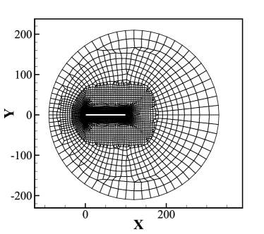
4.5 Rarefied hypersonic flow over a truncated flat plate
The aim of this example is to show the capability of the proposed method to simulate hypersonic flow and to compare it with experimental results. Here, the rarefied hypersonic flow over a flat plate with a truncated leading edge is investigated. Allegre et al. [64] initially conducted this experiment and the freestream conditions given in Table III were used. In this experimental study, a truncated flat plate was positioned at a distance from a nozzle producing a nitrogen flow with a Ma number of 20.2 and a temperature of 13.32 K (the gas constant of nitrogen is ). The plate is 100 mm long, 100 mm wide, and 5 mm thick, and the wall temperature was fixed at 290 K. Two angles of attack (0° and 10°) were examined in this experiment. By using the VHS () model, the gas mean free path is represented as:
| (61) |
The molecular diameter and relative molecular mass of nitrogen are m and g, respectively. As a result, the molecular gas mean free path and the number density are 0.00169 m and , respectively. Meanwhile, by using the length of the plate (100 mm) as the characteristic length, the corresponding Kn number is 0.0169. The reference physical variables and dimensionless physical variables are presented in Tables IV and V, respectively.
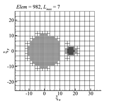
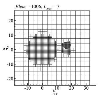
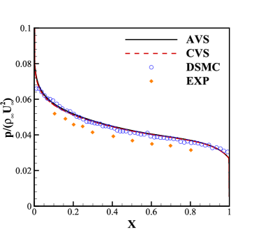
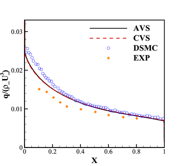
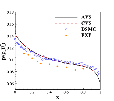
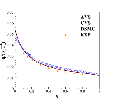
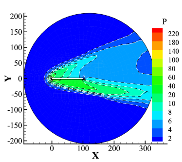
Fig. 21 presents the unstructured physical mesh used for the numerical experiments consist of 8055 cells. And the AVS with the adaptive parameter is shown in Fig. 22. For A0A = 0° and 10°, there are 982 and 1006 elements, respectively. The pressure and heat flux along the lower surface of the plate at A0A = 0° and 10° are shown in Fig. 23 and Fig. 24, And the results are consistent with the results of CVS, which uses a discretized mesh of 101101 points. Furthermore, compared to DSMC, the current heat flux is closer to the result of the experiment. Fig. 25 presents the pressure, horizontal velocity (U), translational and equilibrium temperature contours around the truncated plate at A0A = 10°. The background and white solid lines are the results of the CVS, whereas the black long dash line is the result of the AVS. It is obvious that the results of AVS and CVS are in good agreement with one another.
| Parameter | Value | Unit |
|---|---|---|
| Velocity | 1503 | m/s |
| Temperature | 13.32 | K |
| Density | kg/m | |
| Pressure | 0.0683 | Pa |
| Parameter | Value | Unit |
|---|---|---|
| Velocity | m/s | |
| Temperature | K | |
| Density | kg/m | |
| Length | 1 | mm |
| Parameter | Value |
|---|---|
| Freestream velocity | 16.9 |
| Freestream temperature | 1 |
| Freestream density | 1 |
| Freestream pressure | 0.5 |
| Wall temperature | 21.8 |
| Length | 100 |
4.6 Supersonic flow over a shpere
The performance of the proposed method in the 3D situation is investigated by the simulation of supersonic flow over a sphere. In contrast to the quadtree data structure used for 2D cases, the octree data structure is used for 3D cases. The flow past a sphere is simulated with Rykov model to compare with the experimental drag coefficients [65]. The working gas is nitrogen and the Sutherland formula is using to calculate the viscosity
| (62) |
where the constant are 111K and 124K for nitrogen and air, respectively. According to Eq. 50, the freestream has a total temperature of 300 K and a static temperature of 65.04 K and 43.22 K for Ma 4.25 and 5.45. And the wall temperatures for Ma 4.25 and 5.45 are 302 K and 315 K, respectively. The characteristic length in this example is the sphere’s diameter (2mm). The Re numbers range from 9.55 to 210.0 when Ma is 4.25 and from 4.2 to 32.1 when Ma is 5.45.
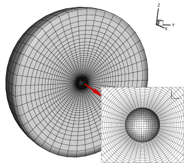
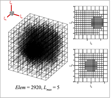
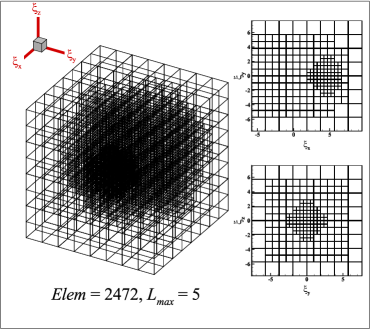
The physical mesh contains 42900 elements is shown in Fig.26 and the height of the first mesh layer at the surface of sphere are 0.01 and 0.04 for Ma 4.25 and 5.45, respectively. For Ma 4.25 and 5.45, the values of the parameter obtained from Eq. 60 are 1.65 and 1.15, respectively. Additionally, the AVS with domain of are shown in Fig. 27, which contain 2472 and 2920 elements for Ma 4.25 and 5.45, respectively. Comparisons of drag coefficients are shown in Table VI and the maximum relative error is only 4.8%-less than the general standard specification (5%). It is noteworthy that the Sutherland parameter for the aerodynamic force simulation is 124K because the experiment’s working gas is air.
| Mach | Re | Present | Exp(Air) | Relative error(%) |
| 4.25 | 9.55 | 2.304 | 2.42 | -4.8 |
| 19.0 | 2.054 | 2.12 | -3.1 | |
| 53.0 | 1.664 | 1.69 | -1.6 | |
| 80.5 | 1.532 | 1.53 | 0.2 | |
| 150.0 | 1.389 | 1.37 | 1.4 | |
| 210.0 | 1.335 | 1.35 | -1.1 | |
| 5.45 | 4.2 | 2.571 | 2.60 | -1.1 |
| 8.6 | 2.423 | 2.44 | -0.7 | |
| 16.8 | 2.226 | 2.28 | -2.4 | |
| 32.1 | 1.993 | 2.04 | -2.3 |
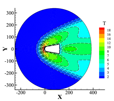
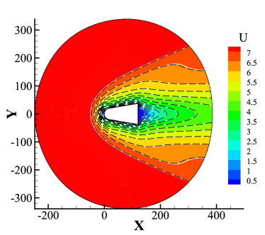
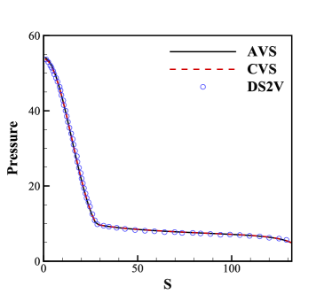
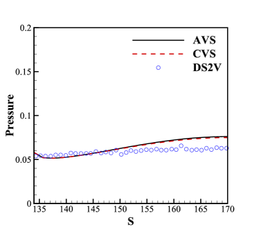
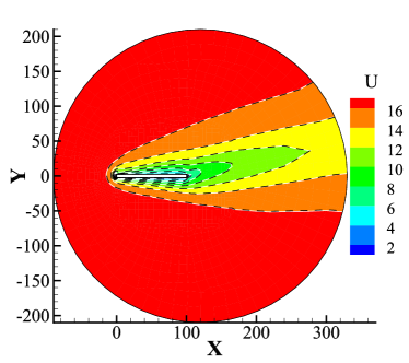
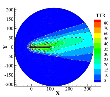
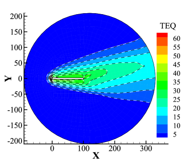
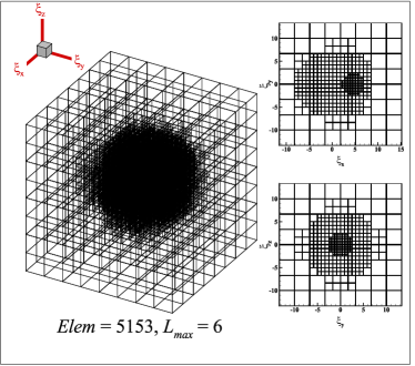
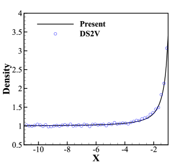
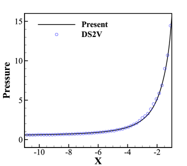
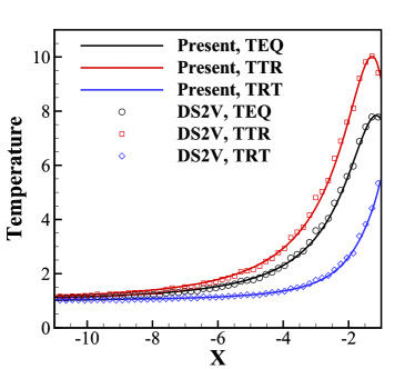
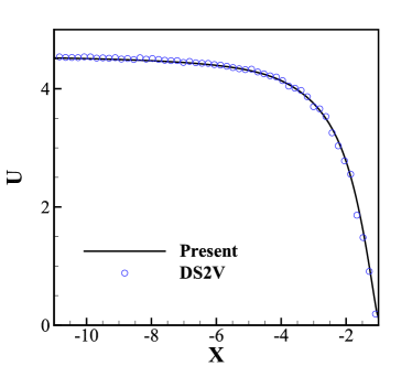
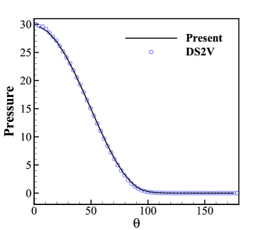
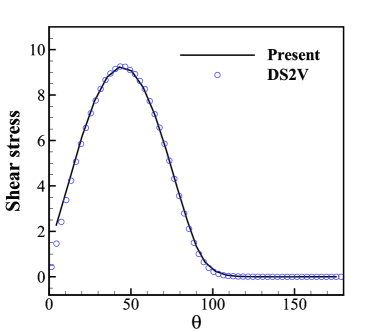
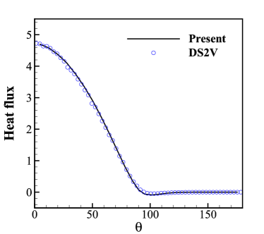
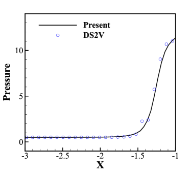
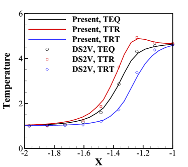
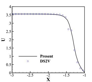
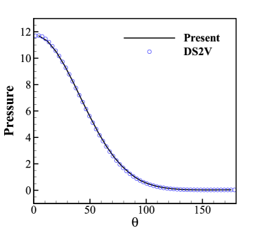
Although the aerodynamic force is satisfactory, the AVS in Fig. 27, whose is only , is imperfect for aerodynamic heat. The ratio of wall temperature to total temperature is 1.007 for Ma 4.25 and 1.050 for Ma 5.45, respectively, showing that the standard deviations and are quite near. This indicates that the radius of the velocity domain is insufficient to cover the stationary zone. Table VII provides further AVS information for Ma 5.45 with varying . Both the numerical results of = and and those of DS2V are in good agreement. With parameters and , the AVS in Fig. 28 has 5133 elements. Figs. 29 and 30 present the physical variables along the central symmetric line in front of the sphere and the sphere’s z = 0 surface at Ma = 5.45 and Re = 4.2. It is clear that there is great agreement between the results of the DS2V and AVS.
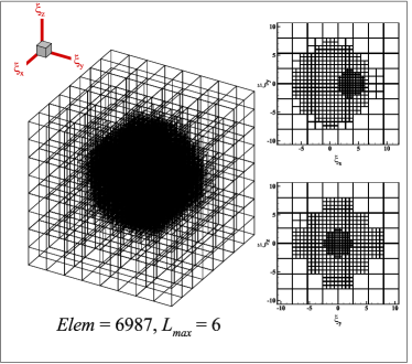
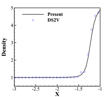
Using the parameters and , the corresponding AVS with 6987 elements is shown in Fig. 31 for the case of Ma = 4.24 and Re = 210. Fig. 32 shows the physical variables along the central symmetric line in front of the sphere, and Fig. 33 shows the physical variables on the sphere’s z = 0 surface. Evidently, there is good agreement between the current results and those from the DS2V. Because nitrogen is the working gas in the DS2V, the Sutherland parameter for the aerodynamic heat simulation is 111 K.
Jiang et al. employed a CVS with elements to simulate the supersonic flow around a sphere in literature [61], which is around 23.6 and 9.9 times as many elements as the AVS in Figs. 27 and 31. It shows how the AVS in this study might greatly reduce the discrete velocity points and enhance computation efficiency. In order to improve the proposed method and achieve even better performance, additional research on the adaptive parameter is required.
| Mach | Elements | |||
|---|---|---|---|---|
| 5.45 | 4 | 0.466 | 0.001 | 3144 |
| 5 | 0.582 | 0.001 | 2108 | |
| 6 | 0.349 | 0.001 | 6784 | |
| 7 | 0.408 | 0.001 | 5174 |
5 Conclusions
In this paper, a global adaptive velocity space approach is proposed, which can automatically update the velocity space with the change of flow. The simplest “consanguinity” relationship is used directly in the reconstruction of VDFs, and the conservation is maintained by the discrete deviation of equilibrium distribution functions. The interpolation of the VDFs at the physical interface and the reconstruction of VDFs between two velocity mesh are avoided thanks to the use of global velocity space and the “consanguinity” relationship, and the high level of parallelism of the program is preserved. The proposed AVS has proved successful for implicit UGKS with simplified multi-scale flux. Additionally, a suitable set of adaptive parameters is constructed, which improves the automation of the method. As a result, the proposed method increases the UGKS’s effectiveness. The global AVS can be used with general explicit and implicit discrete velocity framework. A number of simulations, including 2D and 3D flows, have been carried out to confirm the performance of the global adaptive velocity space.
Acknowledgements
The authors thank Prof. Kun Xu in the Hong Kong University of Science and Technology and Prof. Zhaoli Guo in Huazhong University of Science and Technology for discussions of the UGKS, the DUGKS and multi-scale flow simulations. Jianfeng Chen thanks Dr. Yong Wang in Northwestern Polytechnical University for useful discussions on the adaptive velocity space.
This work was supported by the National Natural Science Foundation of China (Grant Nos. 12172301, 11902266, 12072283, and 11902264) and the 111 Project of China (Grant No. B17037). This work is supported by the high performance computing power and technical support provided by Xi’an Future Artificial Intelligence Computing Center.

References
- [1] G. A. Bird, Molecular gas dynamics and the direct simulation of gas flows, Molecular gas dynamics and the direct simulation of gas flows (1994).
- [2] S. Chen, K. Xu, C. Lee, Q. Cai, A unified gas kinetic scheme with moving mesh and velocity space adaptation, Journal of Computational Physics 231 (20) (2012) 6643–6664.
- [3] L. Zhu, Z. Guo, K. Xu, Discrete unified gas kinetic scheme on unstructured meshes, Computers & Fluids 127 (2016) 211–225.
- [4] T. E. Schwartzentruber, I. D. Boyd, A hybrid particle-continuum method applied to shock waves, Journal of Computational Physics 215 (2) (2006) 402–416.
- [5] T. E. Schwartzentruber, L. C. Scalabrin, I. D. Boyd, Hybrid particle-continuum simulations of hypersonic flow over a hollow-cylinder-flare geometry, AIAA journal 46 (8) (2008) 2086–2095.
- [6] J. M. Burt, I. D. Boyd, A hybrid particle approach for continuum and rarefied flow simulation, Journal of Computational Physics 228 (2) (2009) 460–475.
- [7] Q. Sun, I. D. Boyd, G. V. Candler, A hybrid continuum/particle approach for modeling subsonic, rarefied gas flows, Journal of Computational Physics 194 (1) (2004) 256–277.
- [8] T. E. Schwartzentruber, L. C. Scalabrin, I. D. Boyd, A modular particle–continuum numerical method for hypersonic non-equilibrium gas flows, Journal of Computational Physics 225 (1) (2007) 1159–1174.
- [9] K. Xu, J.-C. Huang, A unified gas-kinetic scheme for continuum and rarefied flows, Journal of Computational Physics 229 (20) (2010) 7747–7764.
- [10] K. Xu, Direct modeling for computational fluid dynamics: construction and application of unified gas-kinetic schemes, Vol. 4, World Scientific, 2014.
- [11] Z. Guo, K. Xu, R. Wang, Discrete unified gas kinetic scheme for all knudsen number flows: Low-speed isothermal case, Physical Review E 88 (3) (2013) 033305.
- [12] Z. Guo, R. Wang, K. Xu, Discrete unified gas kinetic scheme for all knudsen number flows. ii. thermal compressible case, Physical Review E 91 (3) (2015) 033313.
- [13] Z.-H. Li, H.-X. Zhang, Gas-kinetic numerical studies of three-dimensional complex flows on spacecraft re-entry, Journal of Computational Physics 228 (4) (2009) 1116–1138.
- [14] A.-P. Peng, Z.-H. Li, J.-L. Wu, X.-Y. Jiang, Implicit gas-kinetic unified algorithm based on multi-block docking grid for multi-body reentry flows covering all flow regimes, Journal of Computational Physics 327 (2016) 919–942.
- [15] L. Yang, Z. Chen, C. Shu, W. Yang, J. Wu, L. Zhang, Improved fully implicit discrete-velocity method for efficient simulation of flows in all flow regimes, Physical Review E 98 (6) (2018) 063313.
- [16] L. Yang, C. Shu, W. Yang, J. Wu, An improved three-dimensional implicit discrete velocity method on unstructured meshes for all knudsen number flows, Journal of Computational Physics 396 (2019) 738–760.
- [17] W. Sun, S. Jiang, K. Xu, A multidimensional unified gas-kinetic scheme for radiative transfer equations on unstructured mesh, Journal of Computational Physics 351 (2017) 455–472.
- [18] Y. Wang, C. Zhong, S. Liu, et al., Arbitrary lagrangian-eulerian-type discrete unified gas kinetic scheme for low-speed continuum and rarefied flow simulations with moving boundaries, Physical Review E 100 (6) (2019) 063310.
- [19] S. Chen, C. Zhang, L. Zhu, Z. Guo, A unified implicit scheme for kinetic model equations. part i. memory reduction technique, Science bulletin 62 (2) (2017) 119–129.
- [20] Y. Zhu, C. Liu, C. Zhong, K. Xu, Unified gas-kinetic wave-particle methods. ii. multiscale simulation on unstructured mesh, Physics of Fluids 31 (6) (2019) 067105.
- [21] Y. Zhu, C. Zhong, K. Xu, Implicit unified gas-kinetic scheme for steady state solutions in all flow regimes, Journal of Computational Physics 315 (2016) 16–38.
- [22] R. Yuan, C. Zhong, A conservative implicit scheme for steady state solutions of diatomic gas flow in all flow regimes, Computer Physics Communications 247 (2020) 106972.
- [23] W. Sun, S. Jiang, K. Xu, An implicit unified gas kinetic scheme for radiative transfer with equilibrium and non-equilibrium diffusive limits, Communications in Computational Physics 22 (4) (2017) 889–912.
- [24] Q. Zhang, Y. Wang, D. Pan, J. Chen, S. Liu, C. Zhuo, C. Zhong, Unified x-space parallelization algorithm for conserved discrete unified gas kinetic scheme, Computer Physics Communications 278 (2022) 108410.
- [25] S. Chen, Z. Guo, K. Xu, Simplification of the unified gas kinetic scheme, Physical Review E 94 (2) (2016) 023313.
- [26] S. Liu, C. Zhong, Modified unified kinetic scheme for all flow regimes, Physical Review E 85 (6) (2012) 066705.
- [27] M. Zhong, S. Zou, D. Pan, C. Zhuo, C. Zhong, A simplified discrete unified gas kinetic scheme for incompressible flow, Physics of Fluids 32 (9) (2020) 093601.
- [28] M. Zhong, S. Zou, D. Pan, C. Zhuo, C. Zhong, A simplified discrete unified gas–kinetic scheme for compressible flow, Physics of Fluids 33 (3) (2021) 036103.
- [29] L. Zhu, Z. Guo, Numerical study of nonequilibrium gas flow in a microchannel with a ratchet surface, Physical Review E 95 (2) (2017) 023113.
- [30] R. Zhang, S. Liu, C. Zhong, C. Zhuo, Unified gas-kinetic scheme with simplified multi-scale numerical flux for thermodynamic non-equilibrium flow in all flow regimes, arXiv preprint arXiv:2208.14599 (2022).
- [31] J. Chen, S. Liu, Y. Wang, C. Zhong, A compressible conserved discrete unified gas-kinetic scheme with unstructured discrete velocity space for multi-scale jet flow expanding into vacuum environment, Commun. Comput. Phys 28 (2020) 1502–1535.
- [32] Z. Yang, C. Zhong, C. Zhuo, et al., Phase-field method based on discrete unified gas-kinetic scheme for large-density-ratio two-phase flows, Physical Review E 99 (4) (2019) 043302.
- [33] S. Tao, H. Zhang, Z. Guo, L.-P. Wang, A combined immersed boundary and discrete unified gas kinetic scheme for particle–fluid flows, Journal of Computational Physics 375 (2018) 498–518.
- [34] Y. Zhang, L. Zhu, R. Wang, Z. Guo, Discrete unified gas kinetic scheme for all knudsen number flows. iii. binary gas mixtures of maxwell molecules, Physical Review E 97 (5) (2018) 053306.
- [35] W. Sun, S. Jiang, K. Xu, An asymptotic preserving unified gas kinetic scheme for gray radiative transfer equations, Journal of Computational Physics 285 (2015) 265–279.
- [36] Z. Guo, K. Xu, Discrete unified gas kinetic scheme for multiscale heat transfer based on the phonon boltzmann transport equation, International Journal of Heat and Mass Transfer 102 (2016) 944–958.
- [37] D. Pan, C. Zhong, C. Zhuo, W. Tan, A unified gas kinetic scheme for transport and collision effects in plasma, Applied Sciences 8 (5) (2018) 746.
- [38] T. Shuang, S. Wenjun, W. Junxia, N. Guoxi, A parallel unified gas kinetic scheme for three-dimensional multi-group neutron transport, Journal of Computational Physics 391 (2019) 37–58.
- [39] C. Liu, Z. Wang, K. Xu, A unified gas-kinetic scheme for continuum and rarefied flows vi: Dilute disperse gas-particle multiphase system, Journal of Computational Physics 386 (2019) 264–295.
- [40] P. Wang, L.-P. Wang, Z. Guo, Comparison of the lattice boltzmann equation and discrete unified gas-kinetic scheme methods for direct numerical simulation of decaying turbulent flows, Physical Review E 94 (4) (2016) 043304.
- [41] R. Zhang, C. Zhong, S. Liu, C. Zhuo, Large-eddy simulation of wall-bounded turbulent flow with high-order discrete unified gas-kinetic scheme, Advances in Aerodynamics 2 (1) (2020) 1–27.
- [42] V. Titarev, Numerical modeling of high-speed rarefied gas flows over blunt bodies using model kinetic equations, European Journal of Mechanics-B/Fluids 64 (2017) 112–117.
- [43] J. Chen, S. Liu, Y. Wang, C. Zhong, Conserved discrete unified gas-kinetic scheme with unstructured discrete velocity space, Physical Review E 100 (4) (2019) 043305.
- [44] V. Aristov, Method of adaptative meshes in velocity space for the intense shock wave problem, USSR J. Comput. Math. Math. Phys 17 (4) (1977) 261–267.
- [45] C. Baranger, J. Claudel, N. Hérouard, L. Mieussens, Locally refined discrete velocity grids for deterministic rarefied flow simulations, in: AIP Conference Proceedings, Vol. 1501, American Institute of Physics, 2012, pp. 389–396.
- [46] C. Baranger, J. Claudel, N. Hérouard, L. Mieussens, Locally refined discrete velocity grids for stationary rarefied flow simulations, Journal of Computational Physics 257 (2014) 572–593.
- [47] R. R. Arslanbekov, V. I. Kolobov, A. A. Frolova, Kinetic solvers with adaptive mesh in phase space, Physical Review E 88 (6) (2013) 063301.
- [48] V. Kolobov, R. Arslanbekov, Towards adaptive kinetic-fluid simulations of weakly ionized plasmas, Journal of Computational Physics 231 (3) (2012) 839–869.
- [49] F. Bernard, A. Iollo, G. Puppo, A local velocity grid approach for bgk equation, Communications in Computational Physics 16 (4) (2014) 956–982.
- [50] S. Brull, L. Mieussens, Local discrete velocity grids for deterministic rarefied flow simulations, Journal of Computational Physics 266 (2014) 22–46.
- [51] P. L. Bhatnagar, E. P. Gross, M. Krook, A model for collision processes in gases. i. small amplitude processes in charged and neutral one-component systems, Physical review 94 (3) (1954) 511.
- [52] E. Shakhov, Generalization of the krook kinetic relaxation equation, Fluid dynamics 3 (5) (1968) 95–96.
- [53] L. H. Holway Jr, New statistical models for kinetic theory: methods of construction, The physics of fluids 9 (9) (1966) 1658–1673.
- [54] V. Rykov, A model kinetic equation for a gas with rotational degrees of freedom, Fluid Dynamics 10 (6) (1975) 959–966.
- [55] J. Yang, J. Huang, Rarefied flow computations using nonlinear model boltzmann equations, Journal of Computational Physics 120 (2) (1995) 323–339.
- [56] S. E. Rogers, Comparison of implicit schemes for the incompressible navier-stokes equations, AIAA journal 33 (11) (1995) 2066–2072.
- [57] L. Yuan, Comparison of implicit multigrid schemes for three-dimensional incompressible flows, Journal of Computational Physics 177 (1) (2002) 134–155.
- [58] V. Venkatakrishnan, Convergence to steady state solutions of the euler equations on unstructured grids with limiters, Journal of Computational Physics 118 (1) (1995) 120–130.
- [59] J. Chen, S. Liu, C. Zhong, Y. Wang, C. Zhuo, Y. Yang, A gas-surface interaction algorithm for discrete velocity methods in predicting rarefied and multi-scale flows, Available at SSRN 4236130.
- [60] U. Ghia, K. N. Ghia, C. T. Shin, High-re solutions for incompressible flow using the navier-stokes equations and a multigrid method, Journal of Computational Physics 48 (3) (1982) 387–411.
- [61] D. Jiang, M. Mao, J. Li, X. Deng, An implicit parallel ugks solver for flows covering various regimes, Advances in Aerodynamics 1 (1) (2019) 1–24.
- [62] N. Tsuboi, Y. Matsumoto, Experimental and numerical study of hypersonic rarefied gas flow over flat plates, AIAA journal 43 (6) (2005) 1243–1255.
- [63] S. Liu, P. Yu, K. Xu, C. Zhong, Unified gas-kinetic scheme for diatomic molecular simulations in all flow regimes, Journal of Computational Physics 259 (2014) 96–113.
- [64] J. Allegre, M. Raffin, A. Chpoun, L. Gottesdiener, Rarefied hypersonic flow over a flat plate with truncated leading edge, Rarefied gas dynamics: Space science and engineering (1994) 285–295.
- [65] J. F. Wendt, Drag coefficients of spheres in hypersonic non-continuum flow., Tech. rep., VON KARMAN INST FOR FLUID DYNAMICS RHODE-SAINT-GENESE (BELGIUM) (1971).