Morphology of Shocked Lateral Outflows in Colliding Hydrodynamic Flows

Abstract

Supersonic interacting flows occurring in phenomena such as protostellar jets give rise to strong shocks, and have been demonstrated in several laboratory experiments. To study such colliding flows, we use the AstroBEAR AMR code to conduct hydrodynamic simulations in three dimensions. We introduce variations in the flow parameters of density, velocity, and cross sectional radius of the colliding flows in order to study the propagation and conical shape of the bow shock formed by collisions between two, not necessarily symmetric, hypersonic flows. We find that the motion of the interaction region is driven by imbalances in ram pressure between the two flows, while the conical structure of the bow shock is a result of shocked lateral outflows (SLOs) being deflected from the horizontal when the flows are of differing cross-section.

I Introduction

Radiative shocks occur in a variety of settings, such as High Energy Density Plasma (HEDP), protostellar jets (Raga and Kofman, 1992), supernova explosions (Wheeler, Meier, and Wilson, 2002), gamma ray bursts (Piran, 2004), and active galactic nuclei (Rees, 1978). Over the years several efforts have been made to study these phenomena in the laboratory. Despite large differences in physical scale, results obtained in the laboratory can be used to understand phenomena in the astrophysical setting, thanks to the use of dimensionless parameters (Ryutov, Drake, and Remington, 2000; Ryutov et al., 2001; Falize, Michaut, and Bouquet, 2011). Experiments at Imperial College London have produced single flows using a pulsed-power generator to drive radial wire arrays (Lebedev et al., 2005) and radial foils (Suzuki-Vidal et al., 2009; Ciardi et al., 2009); similar experiments have also been performed at Cornell University (Gourdain et al., 2010). Collimation of these flows was driven by toroidal magnetic fields in a manner consistent with the “Magnetic Tower” model (Lynden-Bell, 1996). Extending this work, Suzuki-Vidal et al. (2012) found that the presence of an ambient medium results in the formation of a shock, driven by ablation of halo plasma.

While astronomical shocks are generally produced via time-variations in velocity, a similar effect can be obtained in a laboratory setting by creating a collision between two supersonic flows. Suzuki-Vidal et al. (2015) conducted such an experiment, images of which are shown in figure 1. Among the results of that study are the emergence of small scale structures behind a conical bow shock, which was observed to propagate in a downward direction.

When two flows collide, an interaction region forms, with the jet shocks becoming the boundaries. This region usually consists of a cooling region, in which gas cools from post-shock temperature $T_{s}$ immediately behind the jet shocks to a lower temperature further behind the shock. After passing through the cooling region, gas reaches its final post-cooling temperature and is deposited onto the cold slab, where densities are highest (see figure 1), some shocked material gets ejected laterally by the high pressures throughout the interaction region, producing shocked lateral outflows (SLOs) (Falle and Raga, 1993).

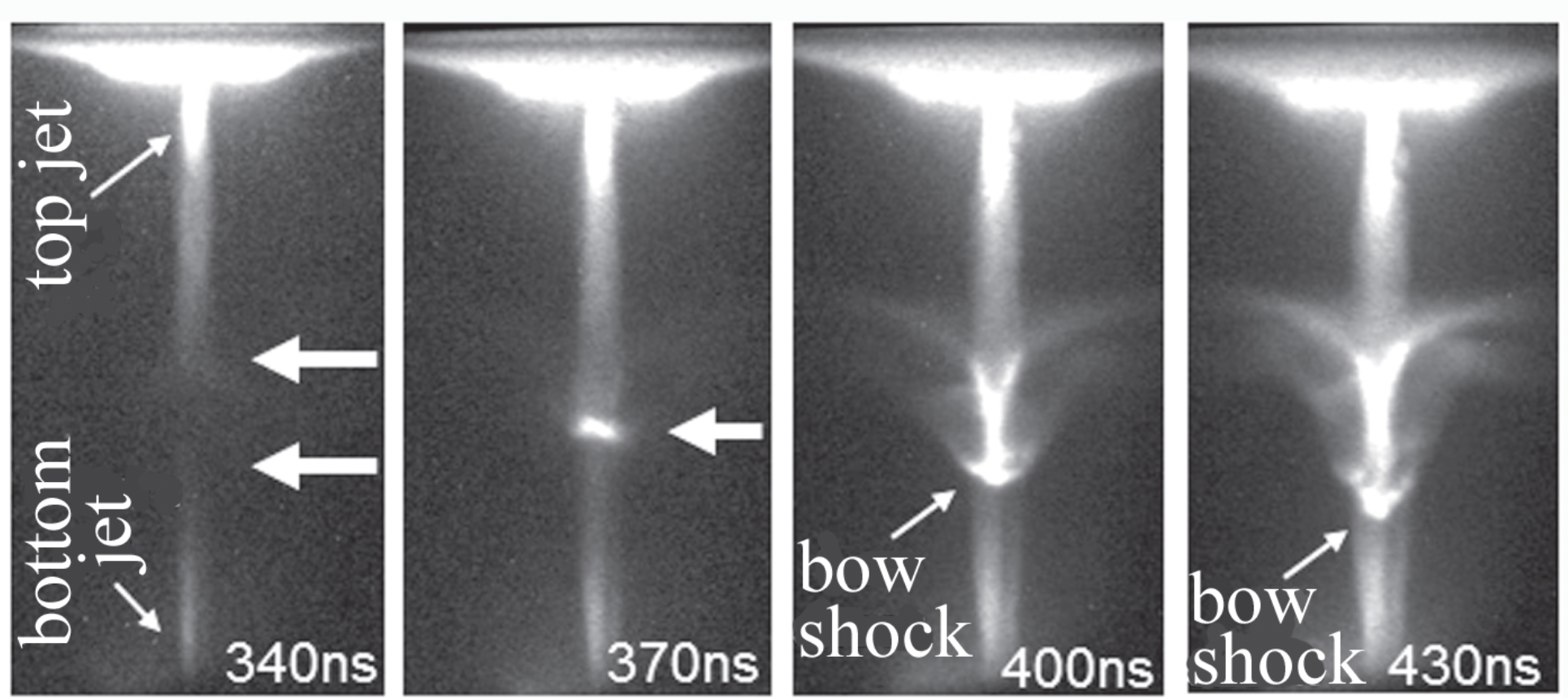
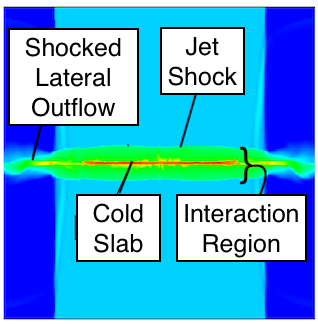
Figure 1: (left) Images of a colliding flow experiment. Adapted from figure 2 of Suzuki-Vidal et al. (2015).
(right) a diagram showing the structure of colliding flows; adapted from Markwick et al. (2021)

In our previous paper (Markwick et al., 2021) we began a series of simulations in an effort to study colliding radiative flows like those of Suzuki-Vidal et al. (2015). In that paper we used hydrodynamic simulations with an analytic form of radiative cooling, focusing our attention on instabilities in an effort to explain the origin of small scale structures. While Suzuki-Vidal et al. (2015) had suggested that the Field (1965) instability was a source of structure, we did not see any evidence of this mode present in the case of analytic cooling. Instead, long-term evolution was found to be dominated by the bending modes characteristic of the nonlinear thin shell instability (NTSI) (Vishniac, 1994), which could be triggered either by sufficiently short cooling lengths or by oscillations resulting from the radiative shock instability (Langer, Chanmugam, and Shaviv, 1981).

In this paper, we continue to investigate the results of Suzuki-Vidal et al. (2015) by extending the results of Markwick et al. (2021). Here we shift our focus away from instabilities (which were discussed in significant depth in Markwick et al. (2021)) to a study of flow parameter variation, allowing us to better understand the conical shape and downward propagation of the bow shock and lateral outflows. We will continue to focus solely on hydrodynamic simulations, but the analytic cooling curve previously used will be replaced with a more realistic cooling function; this will be described in further detail in section II. Our approach of continuing to remain in the radiative hydrodynamic case for now will eventually allow us to have a better understanding of the magnetic case by providing a reference for comparison.

This paper is organized as follows: In Section II we discuss the model system, the selected cooling function, and simulation parameters. In section III, we present the results of the simulations. Section IV will include a discussion of motion of the interaction region, properties of the cold slab, and deflection of the SLOs.

II Methods and Model

The simulations in this study were conducted using AstroBEAR^, (Cunningham et al., 2009; Carroll-Nellenback et al., 2013), which is a massively parallelized adaptive mesh refinement (AMR) code that includes a variety of multiphysics solvers, such as magnetic resistivity, radiative transport, self-gravity, heat conduction, and ionization dynamics. Our study uses only the hydro solvers with an energy source term associated with the radiative cooling. Thus our governing equations are;

$$\frac{\partial\rho}{\partial t}+\boldsymbol{\nabla}\cdot\rho\boldsymbol{v}=0$$ (1)

$$\frac{\partial\rho\boldsymbol{v}}{\partial t}+\boldsymbol{\nabla}\cdot\left(\rho\boldsymbol{v}\otimes\boldsymbol{v}\right)=-\nabla p$$ (2)

$$\frac{\partial E}{\partial t}+\boldsymbol{\nabla}\cdot((E+p)\boldsymbol{v})=-n^{2}\Lambda(n,T)$$ (3)

where $\rho$ is the mass density, $n$ is the number density of nuclei, $\boldsymbol{v}$ is the fluid velocity, $p$ is the thermal pressure, and $E=\frac{1}{\gamma-1}p+\frac{1}{2}\rho v^{2}$ is the combined internal and kinetic energies. $n^{2}\Lambda(n,T)$ is a cooling function, which gives the energy loss per unit volume.

While in (Markwick et al., 2021) we used an analytic cooling function of the form $\Lambda(T)=\alpha\left(\frac{T}{T_{0}}\right)^{\beta}$, in this paper we use a more realistic cooling function. Such a cooling function introduces variation in the slope $\frac{\operatorname{d}\log\Lambda}{\operatorname{d}\log T}$, which is important to both the radiative shock instability and to the Field instability. The specific function $\Lambda(n,T)$ we used was chosen in attempt to provide correspondence with the experiments of Suzuki-Vidal et al. (2015) and is plotted in figure 2. This function was calculated using ABAKO/RAPCAL (Rodríguez et al., 2008; Florido et al., 2009). The required atomic data were obtained using FAC (Gu, 2008), while the resulting function was parameterized in terms of density and temperature using PARPRA (Rodriguez et al., 2014). Cooling is strongest at high temperatures and lower densities; as a fluid cools, $\Lambda(n,T)$ decreases until a local minimum is encountered at a temperature on the order of 10 eV. Cooling then increases again as temperature continues to decrease, but this effect is reduced at higher densities.

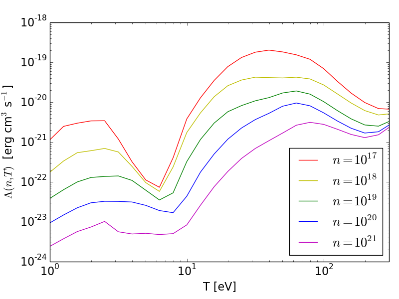
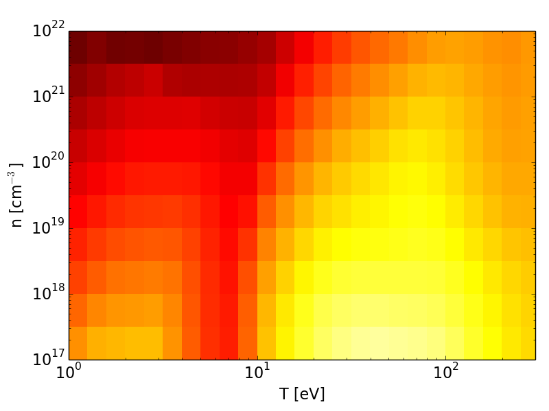
Figure 2: The cooling function plotted (top) as a function of temperature, for selected densities, and (bottom) as a colour-map in terms of density and temperature.

Similarly to Markwick et al. (2021), we drove two cylindrical jets, one from the top and bottom z-boundaries respectively. For the first run, both jets had densities of $3.0\times 10^{18}$ particles per cm³, speeds of 70.0 km s^-1, temperature of 720 K, and cross sectional radii of 1.5 mm. The ambient medium density was $1\times 10^{18}$ particles per cm³ at a temperature of 4320 K. Extrapolated boundary conditions were used in all directions.

Runs were conducted in a 6.4mm cubic space, and consisted of the reference run described above and nine other runs in which jet parameters were varied as follows (summarised in table 1). For the first two runs, we changed the density of the bottom jet to $2.0\times 10^{18}$ and $1.0\times 10^{18}$ particles per cm³. For third and fourth runs, the radius of the bottom jet was varied to 2.0 and 1.0 mm, and the density was varied to $1.69\times 10^{18}$ and $6.75\times 10^{18}$ particles per cm³ such that the mass of the jets remained unaltered. For the fifth and sixth runs, the radius of the bottom jet was varied to 2.0 and 1.0 mm, but this time the density of the jet was reverted to the original value. Finally, the seventh and eighth runs varied velocities of the top and bottom jets to 80 and 60 km s^-1 respectively; these values were chosen to match the experiments in Suzuki-Vidal et al. (2015). The seventh run retained the densities of the reference run, while the eighth run used densities of $2.63\times 10^{18}$ and $3.50\times 10^{18}$ so that the jets were of equal momentum density, and the ninth run used densities of $2.30\times 10^{18}$ and $4.08\times 10^{18}$ so that the jets were of equal momentum flux.

Run	$n_{\text{jet}}$ ($10^{18}$ cm-3)	$v_{\text{jet}}$ (km s-1)	$r_{\text{jet}}$ (mm)	Figures
0	3.00/3.00	70/70	1.5 / 1.5	3-6
1	3.00/2.00	70/70	1.5 / 1.5	4
2	3.00/1.00	70/70	1.5 / 1.5	4
3	3.00/1.69	70/70	1.5 / 2.0	5
4	3.00/6.75	70/70	1.5 / 1.0	5
5	3.00/3.00	70/70	1.5 / 2.0	6
6	3.00/3.00	70/70	1.5 / 1.0	6
7	3.00/3.00	80/60	1.5 / 1.5	7
8	2.63/3.50	80/60	1.5 / 1.5	7
9	2.30/4.08	80/60	1.5 / 1.5	7,8

Table 1: Densities, velocities, and radii of jets in the first set of runs. For each pair of numbers, the first describes the top jet while the second describes the bottom jet.

III Results

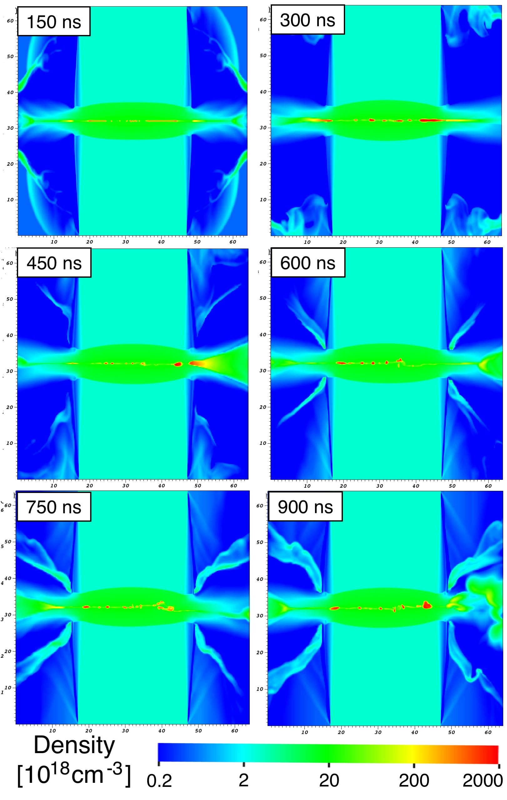
Figure 3: This and all subsequent figures (except as noted) show logarithmic density midplane slices, with the major tick marks placed at intervals of 1mm. For this figure, the reference run (run 0 in table 1) is shown.

We will first examine the reference run (run 0 in table 1), shown in figure 3. This run shows a collision between two identical jets, similar to those studied in Markwick et al. (2021) but now using the complex cooling curve described in section II. As gas crosses the jet shock and enters the interaction region, the density increases from $3\times 10^{18}$ cm^-3 to $1.2\times 10^{19}$ cm^-3. The density varies as the gas cools but remains at the same order of magnitude throughout the cooling region, but is seen to be as high as $2.5\times 10^{21}$ cm^-3 in the cold slab. As gas exits the interaction region through the sides and into the shocked lateral outflows, densities drop to a value of order $1\times 10^{18}$ cm^-3 and lower as gas begins to mix into the ambient medium. At later times clumps are observed to form in the cold slab, though the origin of these is uncertain given that the cold slab is not well resolved at just a few cells ($10^{-3}$ cm) in width. Since the jets are identical, the interaction region remains stationary and shows two identical jet shocks; while the shocks exhibit some curvature, no conical structure is observed. The shocked lateral outflows flow primarily horizontally even though some material leaks from the top and bottom of the SLOs.

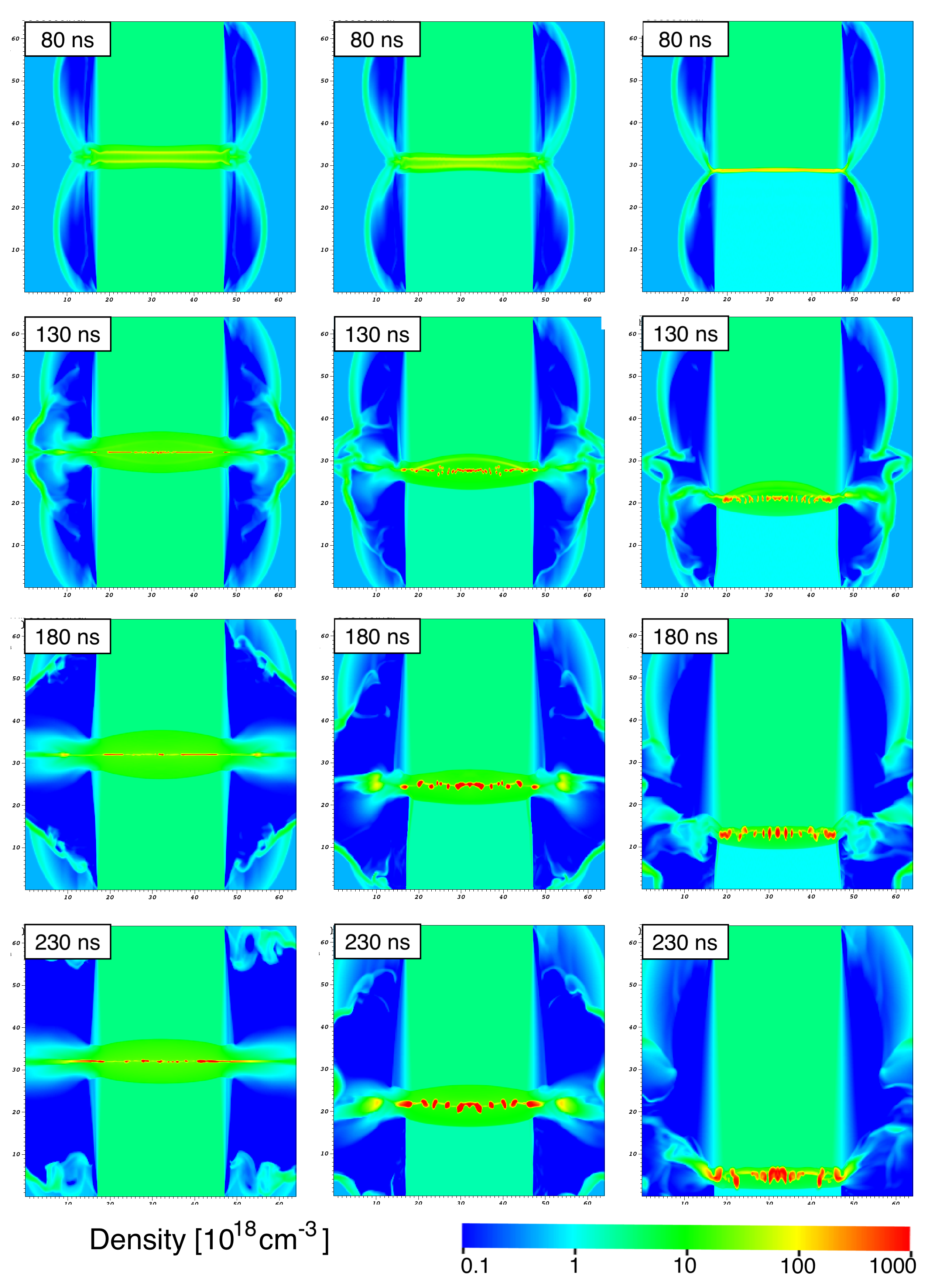
Figure 4: From left to right, runs 0, 1, and 2 from table 1. For these runs, the density of the top jet remains fixed while the density of the bottom jet decreases with each successive run.

Next, we examine cases in which the density of the bottom jet is varied, while the density of the top jet is fixed at $1.0\times 10^{18}$ particles per cm³. Figure 4 shows jets with densities $3.0\times 10^{18},2.0\times 10^{18}$, and $1.0\times 10^{18}$ particles per cm³. As the density of the jets becomes imbalanced, the interaction region no longer remains in place, with the velocity of the interaction region in this case being proportional to the density imbalance. Lateral outflows are seen to be nearly horizontal. Clump formation in the cold slab begins much sooner in collisions with a density imbalance; while the details of smaller structures are beyond the scope of this paper, we conjecture that this is the result of asymmetry exacerbating the formation of perturbations within the cold slab.

Increasing the imbalance further does not significantly change the onset of clump formation. These clumps merge with each other as time progresses, though the regions of cold slab between these clumps is once again not well resolved. Study of the the long term behaviour of these clumps is also limited by the interaction region hitting the wall after a relatively short amount of time.

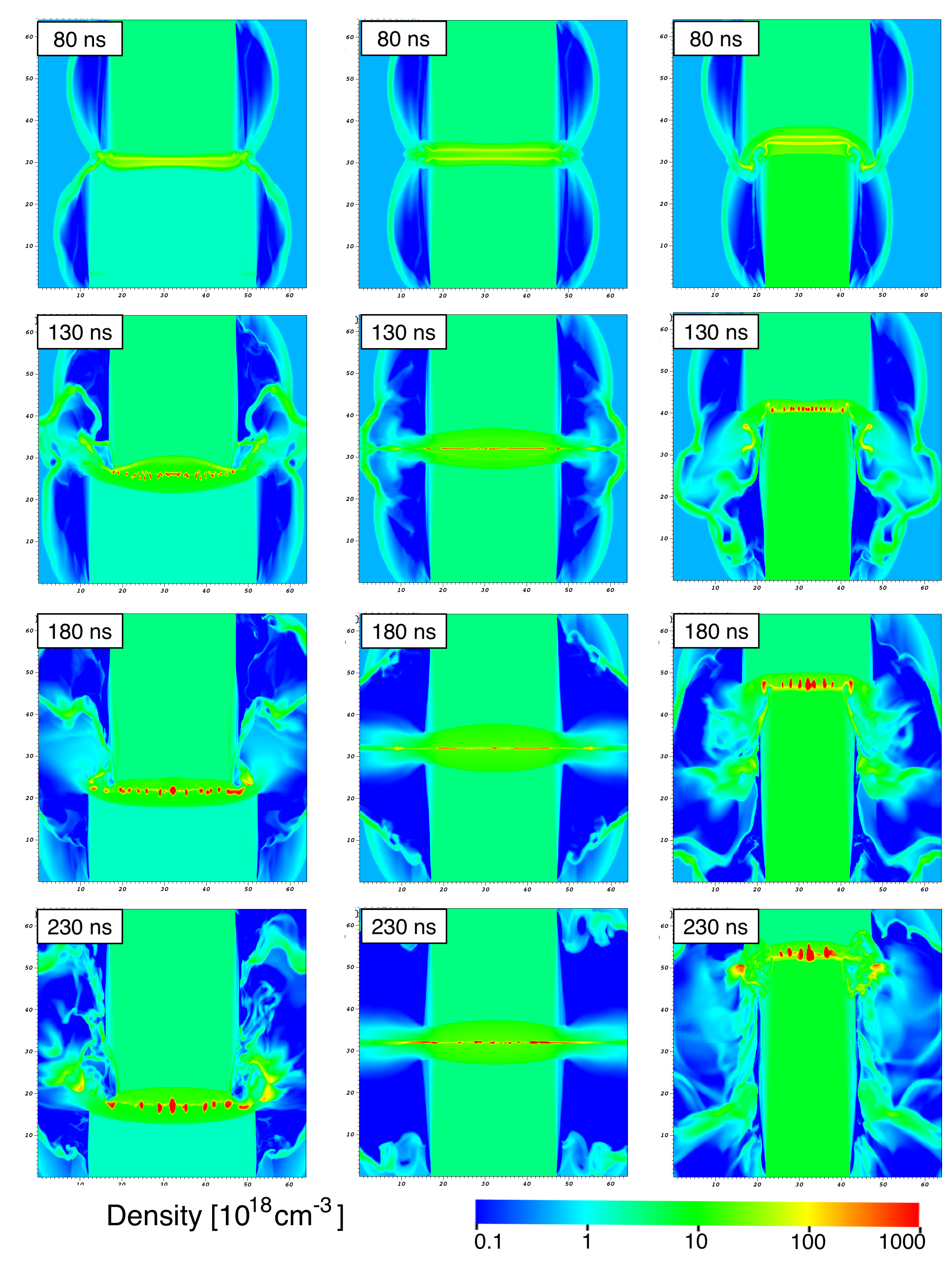
Figure 5: From left to right, runs 3, 0, and 4 from table 1. For these runs, the density and radius of the top jet remains fixed while the bottom jet both increases in density and decreases in radius with each successive run.

Next, we examine cases in which the density of the bottom jet is again varied, this time varying the radius of the bottom jet as $r\propto\rho^{-\frac{1}{2}}$ so that the total mass flux through a horizontal slice remains fixed. Figure 5 shows jets with densities $1.69\times 10^{18},3.0\times 10^{18}$, and $6.75\times 10^{18}$ particles per cm³ and radii 2.0, 1.5, and 1.0 mm. The jet with the smaller radius, having a higher density, drives the motion of the interaction region. As with the previous set, an imbalance of density also results in formation of clumps within the cold slab at earlier times, with these clumps again merging into fewer but larger clumps as time progresses. Since the jets are of differing radii, the SLOs are no longer horizontal, instead bending away from the jet of larger radius.

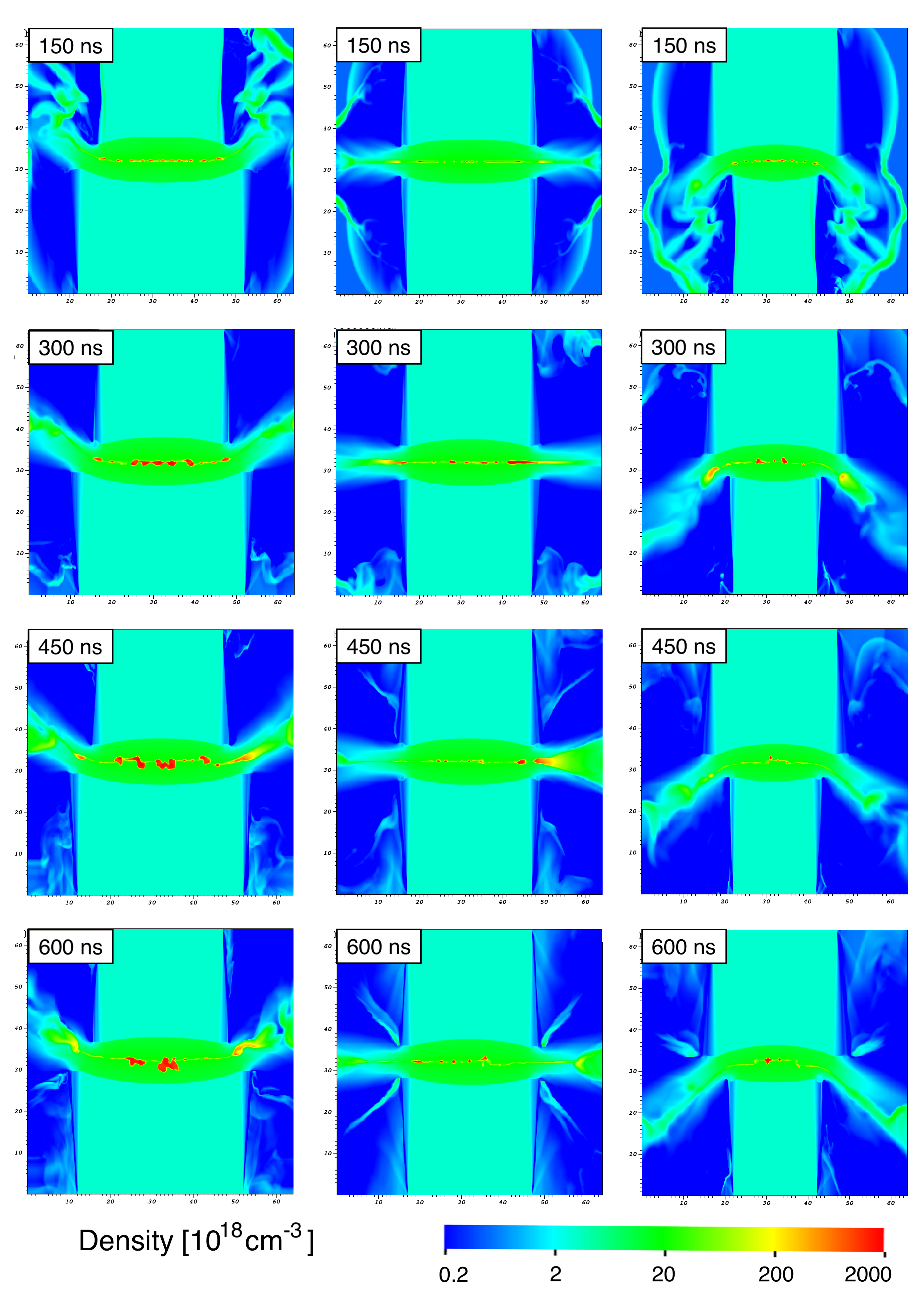
Figure 6: From left to right, runs 5, 0, and 6 from table 1. For these runs, the radius of the top jet remains fixed while the radius of the bottom jet decreases with each successive run.

We next examine cases of equal speed jets for which the radius of the bottom jet is varied at fixed density. Figure 6 shows jets with radii 2.0, 1.5, and 1.0 mm. For equal velocities and equal opposing jet densities, ram pressure is balanced and the interaction region remains at a fixed location. As with density imbalances, an imbalance of radius alone appears to be sufficient to promote earlier clump formation, though in the case with a 1.5 mm jet colliding with a 1.0 mm jet the merging of clumps appears to be inhibited.

Since the speeds and densities are balanced and the interaction region never approaches a wall, these cases can be observed for longer times. After material ejected in the initial collision flies away, a lateral outflow remains. When the jets differ in size, the direction of the SLO occurs at an angle to the horizontal plane and points away from the larger jet. The exact angle increases with the ratio $\frac{(r_{+}^{2}-r_{-}^{2})}{r_{-}}$, where $r_{+}$ and $r_{-}$ are the radii of the larger and smaller jet respectively, and is explored in section IV.4. The interaction region also exhibits curvature, bending away from the larger flow.

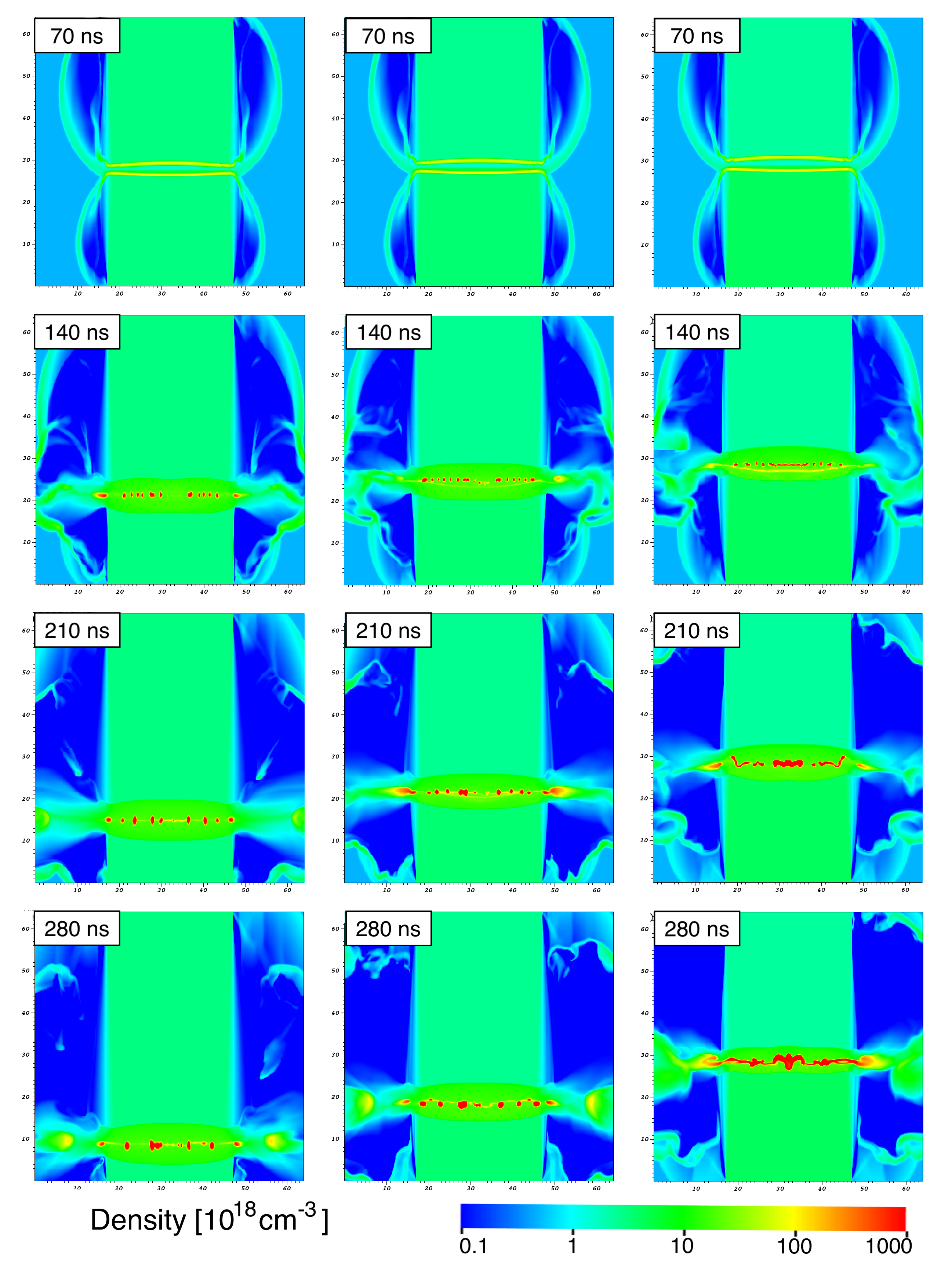
Figure 7: From left to right, runs 7, 8, 9 from table 1. While the previous runs use $v=70$ km s^-1 for both jets, these runs use jet velocities of 80 and 60 km s^-1 for the top and bottom jets respectively. The density of the top jet decreases (and the bottom jet increases) with each successive run.

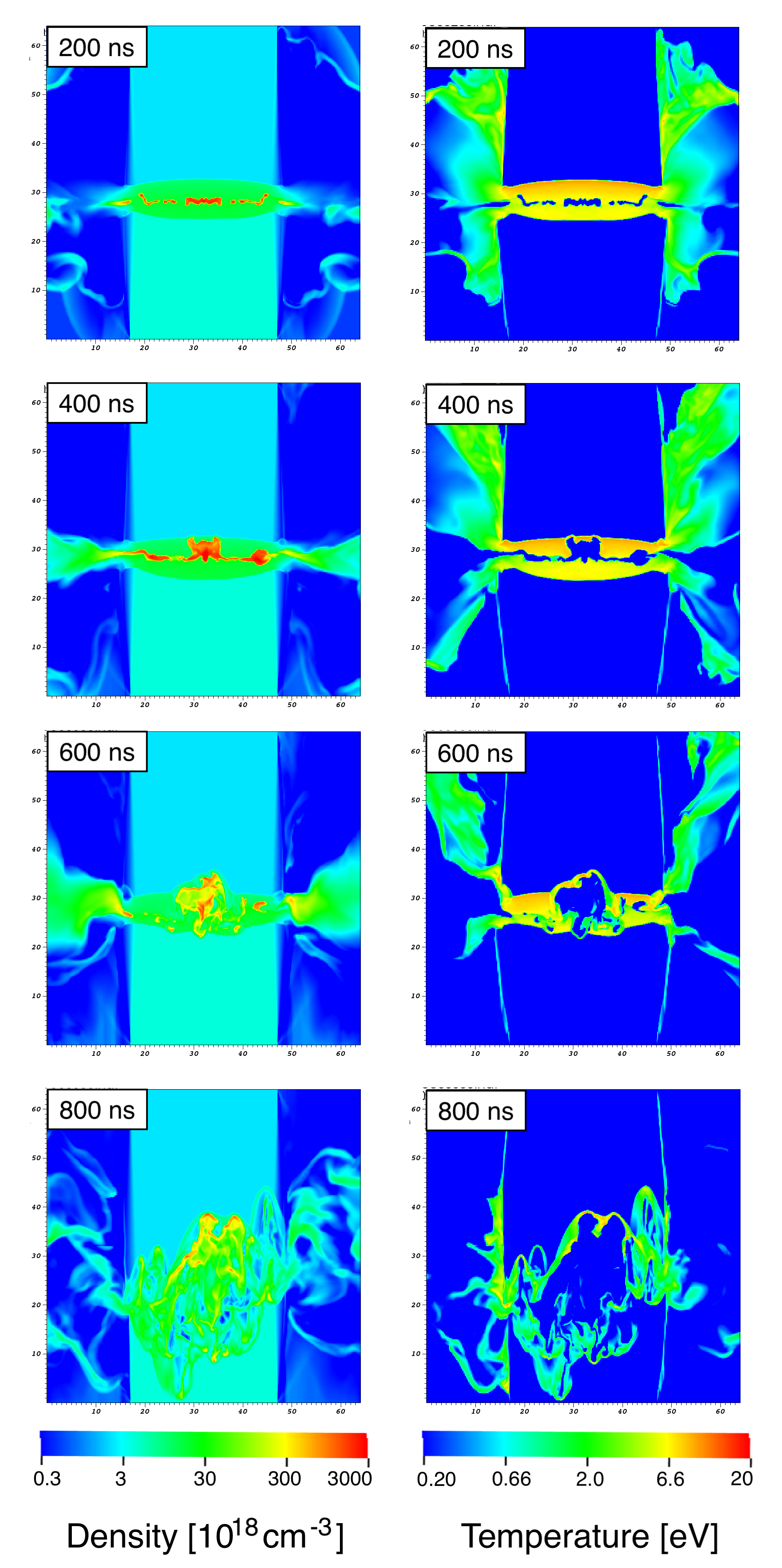
Figure 8: Run 9 from table 1, at intervals of 200 ns. Density is plotted in the left column, while the right column shows a plot of temperature. At later times the Nonlinear Thin Shell Instability can be observed.

Lastly, we examine effects of changing the jet velocity. While previous scenarios used a velocity of 70 km s^-1, the final set of runs uses velocities of 80 km s^-1 for the top jet and 60 km s^-1 for the bottom jet. Figure 7 shows three simulations with these velocities. The first case shows two jets of equal density; here the imbalance of velocity results in the interaction region moving with a velocity of 1̃0 km s^-1 after collision. The second case shows two jets of equal momentum density (and thus equal mass flux); the velocity of the interaction region is significantly reduced, but motion still occurs as a result of ram pressure imbalance. Both of these runs exhibit clumping behaviour similar to that of the runs with a density imbalance. The final case shows two jets of equal ram pressure. The interaction region now remains stationary. While clumping behaviour is initially similar to the other two cases, clump mergers in this case produce a full cold slab spanning the entire radius of the jet. At later times (figure 8), this cold slab is broken apart by the nonlinear thin shell instability, similar to the cases examined in Markwick et al. (2021).

IV Discussion

IV.1 Motion of the Interaction Region

As seen in figures 4, 5, and 7, the interaction region has a nonzero velocity unless the ram pressure $\rho v^{2}$ is equal for both the top and bottom jet. Otherwise, it moves away from the jet with higher ram pressure with velocity $V$. In a reference frame comoving with $V$, the momentum flux entering the interaction region from one jet must balance the momentum flux entering from the other jet. This constraint can be expressed as

$$\rho_{1}\left(v_{1}-V\right)^{2}+p_{1}=\rho_{2}\left(v_{2}-V\right)^{2}+p_{2}$$ (4)

where positive velocities indicate the downward direction; $v_{2}$ is therefore negative. We shall also neglect the thermal pressure difference $p_{1}-p_{2}$.

The requirement that both jets flow into the interaction region produces the constraint $v_{2}<V<v_{1}$. Taking the square root of equation 4, subject to this constraint gives us

$$\sqrt{\rho_{1}}\left(v_{1}-V\right)=\sqrt{\rho_{2}}\left(V-v_{2}\right)$$ (5)

which can be solved for $V$:

$$V=\frac{v_{1}\sqrt{\rho_{1}}+v_{2}\sqrt{\rho_{2}}}{\sqrt{\rho_{1}}+\sqrt{\rho_{2}}}$$ (6)

We will now examine this result in the context of figures 4-7. Velocities can be measured as follows: the location of the cold slab, lower jet shock, and upper jet shock are measured at $t=130$ ns and $t=230$ ns. The positions at each time step are averaged; taking the difference of these averages between the two time steps gives us the displacement (positive is down) over the 100 ns time interval. For runs 7-9, a similar procedure is used except that the measurements are taken at $t=140$ ns and $t=280$ ns. Results are given in table 2.

Run	$n_{1}$	$n_{2}$	$v_{1}$	$v_{2}$	$V$ (eq 6)	$V$ (measured)
0	3.00	3.00	70	70	0	0
1	3.00	2.00	70	70	7.07	6
2	3.00	1.00	70	70	18.8	17
3	3.00	1.69	70	70	9.97	9
4	3.00	6.75	70	70	-14.0	-12
5	3.00	3.00	70	70	0	0
6	3.00	3.00	70	70	0	0
7	3.00	3.00	80	60	10.0	9
8	2.63	3.50	80	60	5.0	5
9	2.30	4.08	80	60	0	0

Table 2: Densities and velocities of the jets in each run, along with the estimated (equation 6) and observed value for the interaction region velocity $V$. All velocities are given in km s^-1 and densities are given in $10^{18}$ cm^-3

We can connect this prediction to the experiments of Suzuki-Vidal et al. (2015), in which the jet velocities were measured to be $v_{1}=80\pm 10$ km s^-1 and $v_{2}=-60\pm 10$ km s^-1. Substantial uncertainties ($\sim 60\%$) were noted for measurements of density, but in any case the ratio $\frac{\rho_{1}}{\rho_{2}}$ was within an order of magnitude of unity. If equation 4 is instead solved for $\frac{\rho_{1}}{\rho_{2}}$ we find

$$\frac{\rho_{1}}{\rho_{2}}=\left(\frac{v_{2}-V}{v_{1}-V}\right)^{2}$$ (7)

The bow shock velocity is stated to be $40\pm 10$ km s^-1, so the density ratio evaluates to $\frac{\rho_{1}}{\rho_{2}}=6.25\pm 4.38$; this on the higher end of what is in agreement with the measurements presented in Suzuki-Vidal et al. (2015).

Another useful quantity to compute for collisions between flows of unequal ram pressure is the Mach number in the centre-of-mass frame. In this paper we define Mach number to be $M^{2}=\frac{\rho v^{2}}{\gamma p}$, and $M_{1}$ and $M_{2}$ to be the Mach numbers for top and bottom flows in the laboratory frame. When combined with equation 6 this definition gives us

$$M^{2}=\frac{\rho_{1}(v_{1}-V)^{2}}{\gamma p_{1}}=\frac{\rho_{1}}{\gamma p_{1}}\left(v_{1}-\frac{v_{1}\sqrt{\rho_{1}}+v_{2}\sqrt{\rho_{2}}}{\sqrt{\rho_{1}}+\sqrt{\rho_{2}}}\right)^{2}$$ (8)

for the centre-of-mass frame (note that Mach numbers must be equal when ram pressures balance). This simplifies to

$$M^{2}=\frac{\rho_{1}\rho_{2}}{\gamma p_{i}}\left(\frac{v_{1}-v_{2}}{\sqrt{\rho_{1}}+\sqrt{\rho_{2}}}\right)^{2}$$ (9)

which, assuming $v_{2}<0<v_{1}$, can be further simplified to

$$M=\frac{M_{1}\sqrt{\rho_{2}}+M_{2}\sqrt{\rho_{1}}}{\sqrt{\rho_{2}}+\sqrt{\rho_{1}}}$$ (10)

Note that while $v_{2}$ is assumed to be negative, we always define the Mach number to be positive. Note that while the interaction region velocity is an average weighed by the square roots of densities, the Mach number is an average weighted by the square roots of inverse densities.

IV.2 Cold Slab in One Dimension

We now begin our examination of shocked lateral outflow by considering a scenario with no outflow: the growth of the cold slab for a flow colliding with a wall in one dimension. In subsequent sections, these results will be useful in the development of a three-dimensional model.

Define $\rho_{i},v_{i}$, and $T_{i}$ to be the initial pre-shock density, velocity, and temperature; also define $\rho_{f},v_{f},$ and $T_{f}$ to be the same values for material in the cold slab. Velocities are specified in a “shock” frame (see figure 9), in which the front (i.e. the side closer to the shock) of the cold slab remains stationary. Any growth of the slab appears in this frame as the far side of the slab moving further away from the shock.

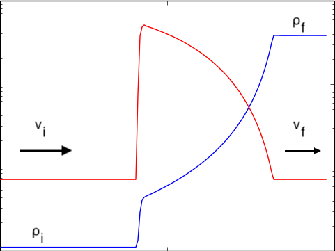
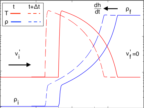
Figure 9: Temperature (red) and Density (blue) for a one dimensional shock in a) the shock frame and b) the lab frame. In the shock frame, the shock remains stationary while material in the cold slab flows away from the shock. In the lab frame, the shock moves to the left (dashed curve) while material already in the cold slab remains stationary.

Let $h$ be the height of the cold slab and $m=\rho_{f}hA$ be the mass of the cold slab within area $A$. Mass continuity tells us that $\frac{\operatorname{d}m}{\operatorname{d}t}$ is equal to the incoming mass flux $\rho_{f}v_{f}$ times the area $A$, so

$$\rho_{f}v_{f}A=\rho_{f}A\frac{\operatorname{d}h}{\operatorname{d}t}+Ah\frac{\operatorname{d}\rho_{f}}{\operatorname{d}t}$$ (11)

which can be solved for $\frac{\operatorname{d}h}{\operatorname{d}t}$

$$\frac{\operatorname{d}h}{\operatorname{d}t}=v_{f}-\frac{h}{\rho_{f}}\frac{\operatorname{d}\rho_{f}}{\operatorname{d}t}$$ (12)

. Going forward we shall assume that $\rho_{f}$ reaches a constant value once $h$ reaches an appreciable length, allowing us to neglect the $\frac{h}{\rho_{f}}\frac{\operatorname{d}\rho_{f}}{\operatorname{d}t}$ term; we therefore conclude that the rate of growth of the slab is equal to the velocity of fluid flow within the slab. With no way for material to exit the slab, the slab will grow indefinitely.

We now establish a relation between the preshock and cold slab states. Conservation of momentum requires that

$$\rho_{i}v_{i}^{2}+p_{i}=\rho_{f}v_{f}^{2}+p_{f}$$ (13)

Using mass continuity $\rho_{i}v_{i}=\rho_{f}v_{f}$ gives

$$v_{f}\left(v_{i}^{2}+\frac{p_{i}}{\rho_{i}}\right)=v_{i}\left(v_{f}^{2}+\frac{p_{f}}{\rho_{f}}\right)$$ (14)

Under the assumption of an isothermal shock ($\frac{p_{f}}{\rho_{f}}=\frac{p_{i}}{\rho_{i}}$), this has two solutions: $v_{f}=v_{i}$ (preshock), and $v_{f}=\frac{p_{i}}{\rho_{i}v_{i}}$ (cold slab). For the latter solution mass continuity then gives

$$\rho_{f}=\frac{\rho_{i}v_{i}}{v_{f}}=\frac{\rho_{i}^{2}v_{i}^{2}}{p_{i}}.$$ (15)

Since the Mach number in the shock frame is defined as $M^{2}=\frac{\rho v_{i}^{2}}{\gamma p_{i}}$, we can express the state of the cold slab as

$$\frac{\rho_{f}}{\rho_{i}}=\frac{p_{f}}{p_{i}}=\frac{v_{i}}{v_{f}}=\gamma M^{2}.$$ (16)

We can apply this result to estimate the density of the cold slab in our simulations; we will do this for run 0. The density of the incoming flow is $3\times 10^{18}$ cm^-3 while the incoming pressure is $2.98\times 10^{5}$ erg cm^-3. Using a mass of 1 amu, we find a sound speed of 3.15 km s^-1, which for a jet velocity of 70 km s^-1 gives us a Mach number of 22. This gives us a cold slab density of $2.4\times 10^{21}$ cm^-3, which is in good agreement with what is observed in our simulations.

Before moving on to three dimensions, we briefly discuss this problem in the “lab” frame, which is useful to consider for a flow running into a stationary wall. If we return to figure 9, we see that in this frame the far side of the cold slab remains stationary while the shock moves away from the wall. We therefore can define $v_{i}^{\prime}=v_{i}-v_{f}$ and $M^{\prime}=\frac{v_{i}^{\prime}}{v_{i}}M$ as the preshock velocity and Mach number in this frame. Using this, we find that equation 16 becomes

$$\frac{\rho_{f}}{\rho_{i}}=\frac{p_{f}}{p_{i}}=\frac{v_{i}^{\prime}}{v_{f}}+1=\gamma M^{\prime 2}\left(1+\frac{v_{f}}{v_{i}^{\prime}}\right)^{2}$$ (17)

the solution of which is given by

$$\frac{v_{f}}{v_{i}^{\prime}}=\sqrt{\frac{1}{4}+\frac{1}{\gamma M^{\prime 2}}}-\frac{1}{2},$$ (18a)

and

$$\frac{\rho_{f}}{\rho_{i}}=\gamma M^{\prime 2}\left[\frac{1}{2}+\sqrt{\frac{1}{4}+\frac{1}{\gamma M^{\prime 2}}}\right]+1.$$ (18b)

These expressions can also be derived by considering conservation laws in the lab frame, noting that the mass of any region enclosing the shock increases over time.

IV.3 Cold Slab for Cylindrical flows

We now wish to extend the model developed in the previous section to a cylindrical model in which gas is permitted to escape laterally. Our primary aim in this section is to use mass conservation to estimate the size of the cold slab. Although some gas also escapes from the sides of the cooling regions without ever reaching the cold slab, the cooling region accounts for just 10% of the mass of the interaction despite being around 90% of the volume. We therefore make the approximation that the mass of the SLO originates entirely from the cold slab material. A more accurate calculation could be done by dividing the cooling region into layers and computing the SLO for each layer.

Let $r_{-}$ be the radius of the incoming flow (the reason for labelling as minus will become apparent in the next section). Assume $h$ is the height of our cylinder, and that mass flows into the cylinder from both the top and bottom and out the sides. The outgoing mass flux is equal to $\rho_{h}(2\pi r_{0}h)v_{\perp}$, so equations 11 and 12 become

$$\rho_{f}v_{f}(2\pi r_{-}^{2})-\rho_{h}v_{\perp}(2\pi r_{-}h)=\rho_{f}(\pi r_{-}^{2})\frac{\operatorname{d}h}{\operatorname{d}t}+\pi r_{-}^{2}h\frac{\operatorname{d}\rho_{f}}{\operatorname{d}t}$$ (19a)

$$\frac{\operatorname{d}h}{\operatorname{d}t}=2v_{f}-\frac{h}{\rho_{f}}\frac{\operatorname{d}\rho_{f}}{\operatorname{d}t}-\frac{\rho_{h}(2\pi r_{-}h)}{\rho_{f}(\pi r_{-}^{2})}v_{\perp}.$$ (19b)

In equilibrium this gives an expression for the SLO velocity

$$v_{\perp}=\frac{\rho_{f}v_{f}r_{-}}{\rho_{h}h}.$$ (20)

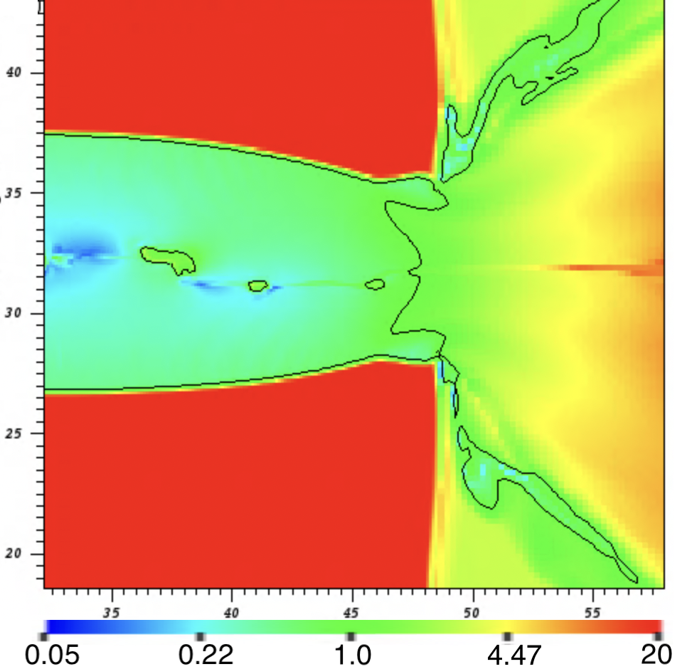
Figure 10: A plot of Mach number near the edge of the interaction region, for run 0 at time 660 ns. A black contour is drawn at $M=1$.

Let us begin by guessing that $\rho_{h}=\rho_{f}$. We will also assume that $v_{\perp}$ is equal to the sound speed (which must equal that of the incoming flows). This is justifiable both theoretically (Falle and Raga, 1993) and by observation of our simulations (see figure 10). We therefore find

$$\frac{v_{i}}{M}=v_{f}\frac{r_{-}}{h}$$ (21)

Since the slab has no net growth we can use equation 16 for $\frac{v_{f}}{v_{i}}$. Solving for $\frac{h}{r_{-}}$ therefore gives us

$$\frac{h}{r_{-}}=\frac{1}{\gamma M}$$ (22)

The actual ratio may be slightly smaller as a result of aforementioned small amount of gas leaking laterally out of the cooling region. The jets in our simulations have $\gamma=\frac{5}{3}$ and $M\sim 20$ so this factor should be approximately 0.03. For a jet of radius 1.5 mm the size of the cold slab would be just 0.045 mm, which is comparable to what we observe. We must note however that such a length corresponds to less than 4 cells on the grid at the highest level of refinement, so numerical errors are likely to be significant.

IV.4 Deflection Angle for Jets with Different Radii

Finally, we shall examine the deflection angle for SLOs produced by jets with different radii. We will assume that the jets are of equal density and velocity. Under these assumptions, the deflection angle can be approximated as the collision between the SLO of a system of identical jets with radius $r_{-}$ (the radius of the smaller jet), and an incoming flow from the larger jet between $r_{-}$ and $r_{+}$ (the radius of the larger jet).

Define angle $\theta$ to be the angle of deflection, relative to the surface normal to the incoming flows of density $\rho_{i}$, speed, $v_{i}$, and pressure $p_{i}$ (see figure 11). Define area $A_{\text{SLO}}\operatorname{d}\varphi$ as the area of some surface which is normal to the SLO and covers the extent of the SLO through angle $\operatorname{d}\varphi$ about the jet axis.

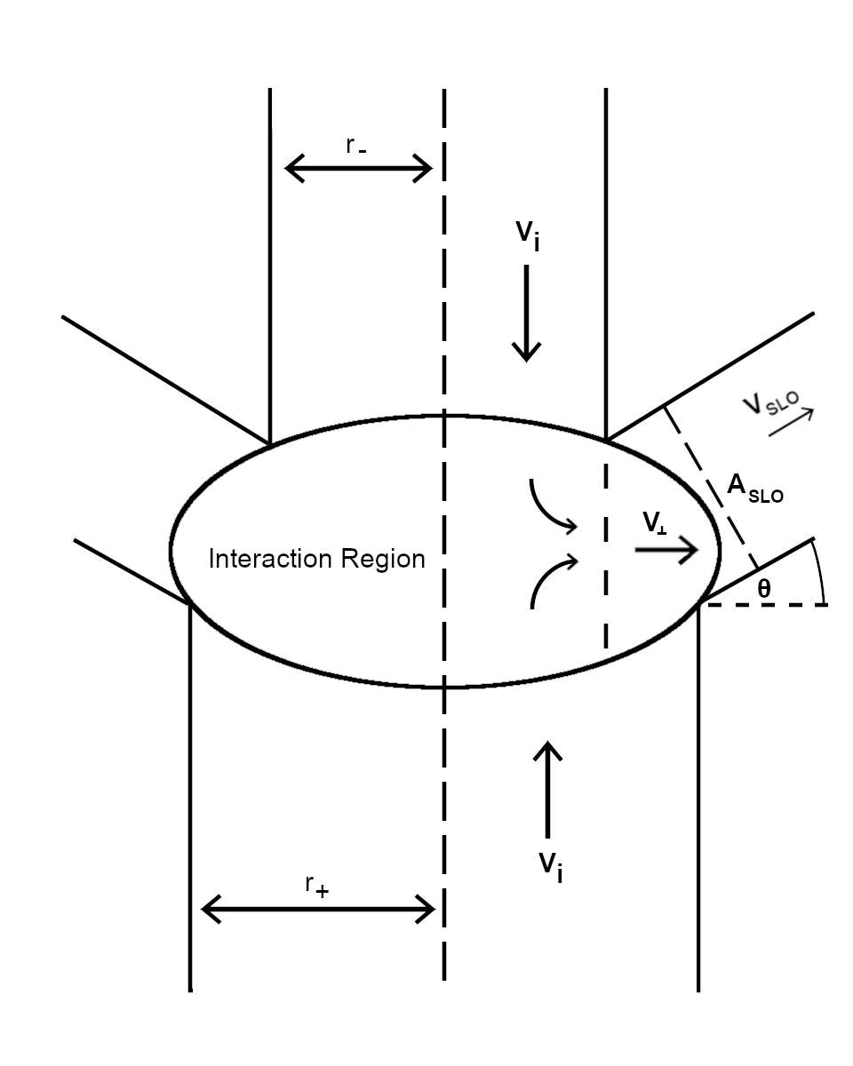
Figure 11: A diagram discussing the geometry of the problem for determining properties of the SLO for multiple jets.

Let the SLO be characterized by $\rho_{\text{SLO}}$, $v_{\text{SLO}}$, and $p_{\text{SLO}}$; note that the SLO subscript denotes material in the deflected SLO, while an $h$ subscript describes a horizontal SLO. The outgoing horizontal and vertical momentum fluxes must therefore be

$$F_{x}=(\rho_{\text{SLO}}v_{\text{SLO}}^{2}+p_{\text{SLO}})A_{\text{SLO}}\cos\theta\operatorname{d}\varphi$$ (23a)

$$F_{y}=(\rho_{\text{SLO}}v_{\text{SLO}}^{2}+p_{\text{SLO}})A_{\text{SLO}}\sin\theta\operatorname{d}\varphi$$ (23b)

We now express the horizontal momentum flux leaving the interaction region in terns if the incoming quantities. The SLO from the collision within the inner radius can be characterized as having density $\rho_{h}=\rho_{f}=\gamma M^{2}\rho_{i}$ and velocity $v_{\perp}=\sqrt{\frac{\gamma p_{i}}{\rho_{i}}}$ (see equation 16 and the discussion in section IV.3). The pressure $p_{h}$ can be estimated using conservation of energy within the cold slab (which features no cooling).

$$\left[\frac{\gamma p_{f}v_{f}}{\gamma-1}+\frac{\rho_{f}v_{f}^{3}}{2}\right](2\pi r_{-}^{2})=\left[\frac{\gamma p_{h}v_{\perp}}{\gamma-1}+\frac{\rho_{h}v_{\perp}^{3}}{2}\right](2\pi r_{-}h)$$ (24)

Note that we use $v_{f}$ (the state of material entering the cold slab) instead of $v_{i}$ as we are only considering energy flux in and out of the cold slab rather than the interaction. Expressing $\rho_{h}$ and $v_{\perp}$ in terms of $\rho_{f},p_{f}$, and $M$ allows us to solve for $p_{h}$

$$p_{h}=\left[\frac{3-\gamma}{2}+\frac{\gamma-1}{2\gamma^{2}M^{2}}\right]p_{f}$$ (25)

Therefore in the limit of high Mach number, the horizontal momentum flux produced by the cold slab is equal to

$$F_{x}^{h}=(\rho_{h}v_{\perp}^{2}+p_{h})(r_{-}h\operatorname{d}\varphi)\approx Mp_{i}\left(\frac{3+\gamma}{2}\right)(r_{-}^{2}\operatorname{d}\varphi)$$ (26)

While neglecting the cooling region is sufficient when considering mass flux, the high pressures found in the cooling region also contribute significantly to the momentum flux. We can however continue to ignore the kinetic term $\rho_{\text{cr}}v_{\perp}^{2}$ as this term approaches a constant in the limit of high Mach number and thus accounts for less than one percent of the momentum flux for collisions with $M\sim 20$. We shall approxmiate the pressure within the cooling region to be equal to the immediate postshock pressure; this pressure within the cooling region should exceed this, but by a factor of less than $\frac{\gamma+1}{2}$ (assuming pressure in the cooling region never exceeds that of the cold slab). We therefore conclude that a lower bound for the contribution of the cooling region to the momentum flux is given by

$$F_{x}^{L}=p_{\text{ps}}(2r_{-}L\operatorname{d}\varphi)=\frac{4\gamma M^{2}\xi}{\gamma+1}p_{i}(r_{-}^{2}\operatorname{d}\varphi)$$ (27)

where $L$ is the (vertical) size of the cooling region and $\xi=\frac{L}{r_{-}}$. In Markwick et al. (2021) we showed how to calculate $L$ for a power-law cooling function as an improvement of the approximation given in Chevalier and Imamura (1982), and a similar approach can be used for a more complex function. While performing such a calculation is necessary if one wishes to predict the outflow angle without running a simulation, when comparing analytical predictions to simulation results we will instead take the approach of measuring $L$ from the simulation results.

In the vertical direction, the incoming jet flux is

$$F_{y}=(\rho_{i}v_{i}^{2}+p_{i})\left(\frac{r_{+}^{2}-r_{-}^{2}}{2}\operatorname{d}\varphi\right)=(\gamma M^{2}+1)p_{i}\left(\frac{r_{+}^{2}-r_{-}^{2}}{2}\right)\operatorname{d}\varphi$$ (28)

Using equations 23 we can deduce $\tan\theta=\frac{F_{y}}{F_{x}^{h}+F_{x}^{L}}$; combining this with equations 26 - 28 allows us to estimate the deflection angle:

$$\tan\theta=\left[\frac{(\gamma+1)(\gamma M^{2}+1)}{8\gamma\xi M^{2}+(\gamma+1)(\gamma+3)M}\right]\frac{r_{+}^{2}-r_{-}^{2}}{r_{-}^{2}}$$ (29)

We now compare equation 29 to our simulations. Using $\gamma=\frac{5}{3}$, $M=20$, $L=0.4$ mm, $r_{-}=1.0$ mm and $r_{+}=1.5$ mm, we find $\tan\theta=0.93$ or $\theta=43^{\circ}$; this is confirmed by the 600 ns frame of figure 6 which shows a deflection angle of $\theta=41^{\circ}$. Meanwhile if we use $r_{-}=1.5$ mm and $r_{+}=2.0$ mm we find $\tan\theta=0.73$ or $\theta=39^{\circ}$, with the measured angle being $36^{\circ}$.

To further test equation 29, we ran an additional set of simulations. These simulations were similar to run 6 (see figure 6), but the radius of the top jet varied between values of 1.0 mm, 1.5 mm, 2.0 mm, and 2.5 mm; these runs were also conducted at lower resolution than the other runs. Using the 1.0 mm case we estimate $\xi=0.3$, and for each subsequent run we took four measurements of deflection angle, shown in magenta in figure 12. We find that equation 29 was very accurate for the 1.5 mm case, but sorely overestimates for $\frac{r_{+}}{r_{-}}\gtrsim 2$. An improved result may be obtained by considering the curvature in the region between $r_{-}$ and $r_{+}$, as equation 29 is best suited to the limit where that region is small.

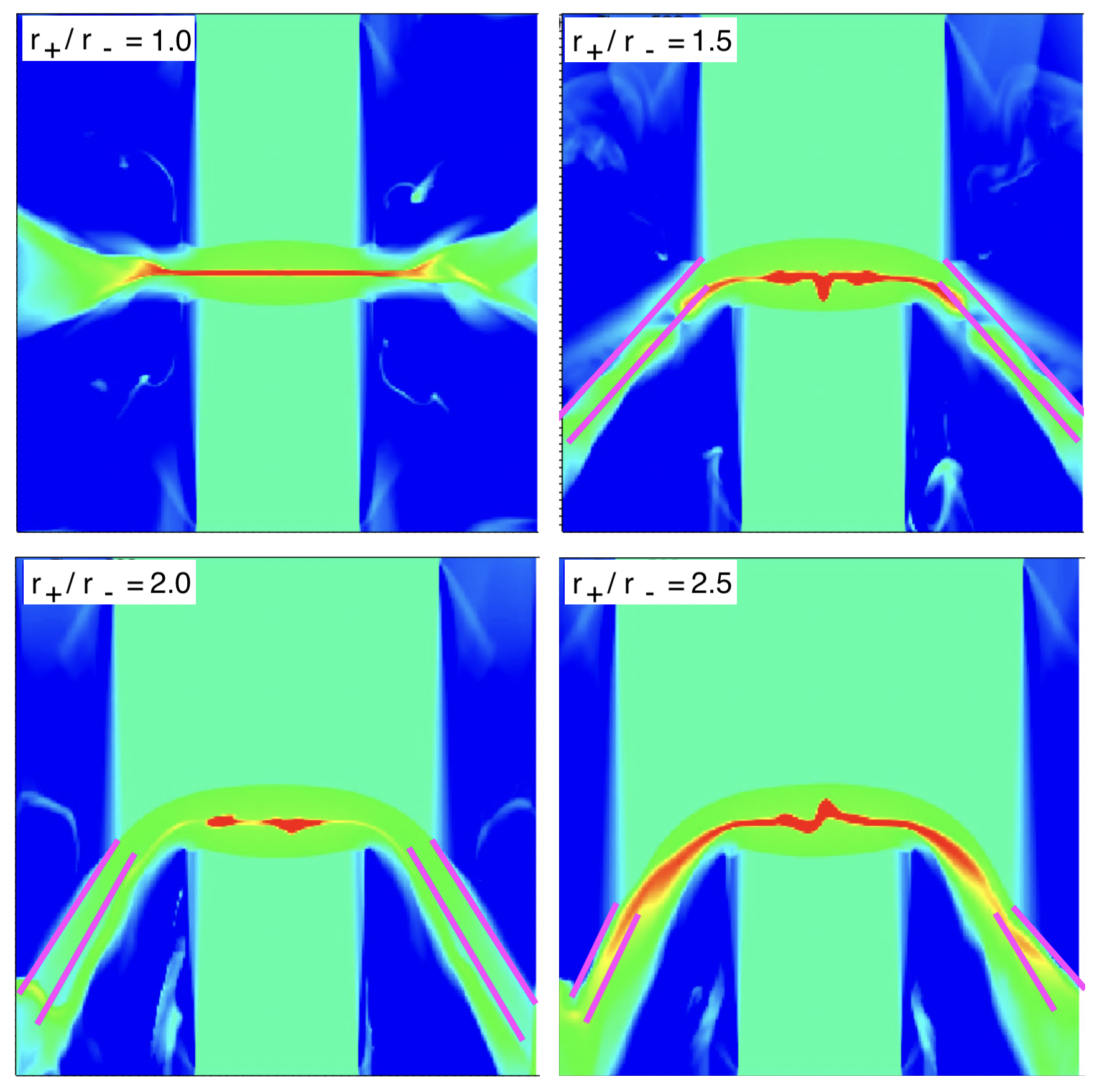
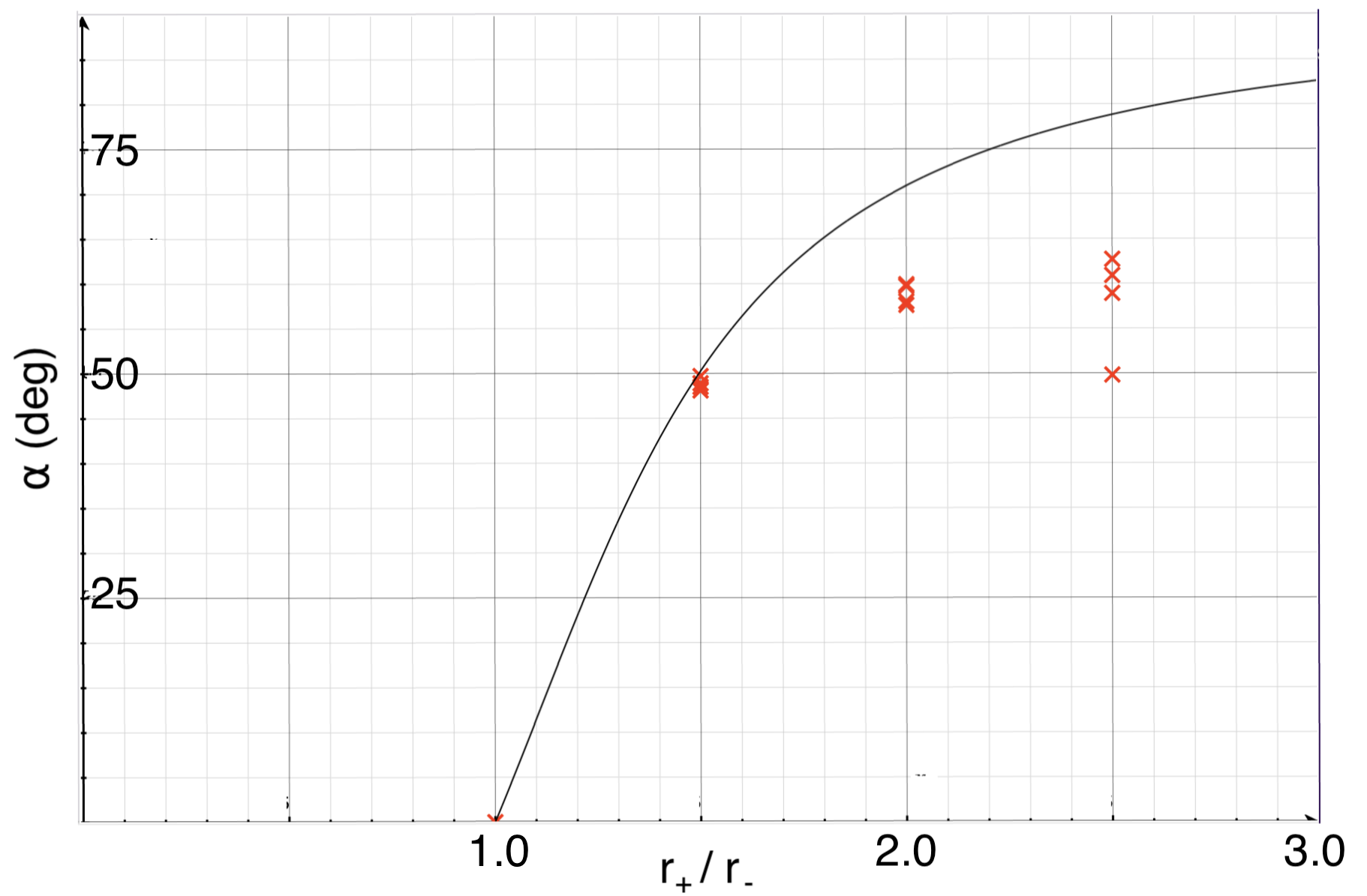
Figure 12: (top) A set of simulations used to further test equation 29. (bottom) Deflection angles vs the ratio of radii. Each red cross corresponds to a magenta line in the simulations, while the black curve is the estimated deflection.

IV.5 Conclusions

In this paper we have continued our studies of colliding flows. While in Markwick et al. (2021) we used identical flows and an analytic cooling model to isolate the effects of instabilities, in this paper we used a more realistic cooling function and variation of flow parameters; this was done in part to bring our simulations closer to the experiments of Suzuki-Vidal et al. (2015) while still remaining the hydrodynamic regime. Our simulations suggest explanations for two important features of the bow shock. First, for flows of differing density or velocity, the interaction region (and thus a shock which bounds it) moves at a speed given by equation 6. Second, we find that the conical shape of the bow shock arises from a mismatch in the cross-sectional radii of the flows, with the shocked lateral outflows being deflected away from the jet of larger radius. All of the simulations in these first two papers have been conducted in the hydrodynamic limit. While this is useful for isolating various aspects of the underlying physics, magnetic fields are likely to be significant in both laboratory and astrophysical flows, and are thus a worthwhile inclusion in future papers on the subject. Effects relating to optical depth may also be worth exploring, particularly in connection to laboratory contexts.

Data Availability Statement

The data that support the findings of this study are available from the corresponding author upon reasonable request.

Author Declarations

The authors have no conflicts to disclose.

References

- Raga and Kofman (1992) A. C. Raga and L. Kofman, “Knots in Stellar Jets from Time-dependent Sources,” Astrophys. J. 386, 222 (1992).
- Wheeler, Meier, and Wilson (2002) J. C. Wheeler, D. L. Meier, and J. R. Wilson, “Asymmetric Supernovae from Magnetocentrifugal Jets,” Astrophys. J. 568, 807–819 (2002), arXiv:astro-ph/0112020 [astro-ph] .
- Piran (2004) T. Piran, “The physics of gamma-ray bursts,” Reviews of Modern Physics 76, 1143–1210 (2004), arXiv:astro-ph/0405503 [astro-ph] .
- Rees (1978) M. J. Rees, “The M87 jet: internal shocks in a plasma beam?” MNRAS 184, 61P–65P (1978).
- Ryutov, Drake, and Remington (2000) D. D. Ryutov, R. P. Drake, and B. A. Remington, “Criteria for Scaled Laboratory Simulations of Astrophysical MHD Phenomena,” Astrophys. J. S. 127, 465–468 (2000).
- Ryutov et al. (2001) D. D. Ryutov, B. A. Remington, H. F. Robey, and R. P. Drake, “Magnetohydrodynamic scaling: From astrophysics to the laboratory,” Physics of Plasmas 8, 1804–1816 (2001).
- Falize, Michaut, and Bouquet (2011) É. Falize, C. Michaut, and S. Bouquet, “Similarity Properties and Scaling Laws of Radiation Hydrodynamic Flows in Laboratory Astrophysics,” Astrophys. J. 730, 96 (2011), arXiv:0910.2338 [astro-ph.SR] .
- Lebedev et al. (2005) S. V. Lebedev, A. Ciardi, D. J. Ampleford, S. N. Bland, S. C. Bott, J. P. Chittenden, G. N. Hall, J. Rapley, C. A. Jennings, A. Frank, E. G. Blackman, and T. Lery, “Magnetic tower outflows from a radial wire array Z-pinch,” MNRAS 361, 97–108 (2005), arXiv:astro-ph/0505027 [astro-ph] .
- Suzuki-Vidal et al. (2009) F. Suzuki-Vidal, S. V. Lebedev, A. Ciardi, S. N. Bland, J. P. Chittenden, G. N. Hall, A. Harvey-Thompson, A. Marocchino, C. Ning, C. Stehle, A. Frank, E. G. Blackman, S. C. Bott, and T. Ray, “Formation of episodic magnetically driven radiatively cooled plasma jets in the laboratory,” ApSS 322, 19–23 (2009), arXiv:0904.0165 [astro-ph.SR] .
- Ciardi et al. (2009) A. Ciardi, S. V. Lebedev, A. Frank, F. Suzuki-Vidal, G. N. Hall, S. N. Bland, A. Harvey-Thompson, E. G. Blackman, and M. Camenzind, “Episodic Magnetic Bubbles and Jets: Astrophysical Implications from Laboratory Experiments,” ApJL 691, L147–L150 (2009), arXiv:0811.2736 [astro-ph] .
- Gourdain et al. (2010) P. A. Gourdain, I. C. Blesener, J. B. Greenly, D. A. Hammer, P. F. Knapp, B. R. Kusse, and P. C. Schrafel, “Initial experiments using radial foils on the cornell beam research accelerator pulsed power generator,” PhPl 17, 012706 (2010).
- Lynden-Bell (1996) D. Lynden-Bell, “Magnetic collimation by accretion discs of quasars and stars,” MNRAS 279, 389–401 (1996).
- Suzuki-Vidal et al. (2012) F. Suzuki-Vidal, M. Bocchi, S. V. Lebedev, G. F. Swadling, G. Burdiak, S. N. Bland, P. de Grouchy, G. N. Hall, A. J. Harvey-Thompson, E. Khoory, S. Patankar, L. Pickworth, J. Skidmore, R. Smith, J. P. Chittenden, M. Krishnan, R. E. Madden, K. Wilson-Elliot, A. Ciardi, and A. Frank, “Interaction of a supersonic, radiatively cooled plasma jet with an ambient medium,” Physics of Plasmas 19, 022708 (2012).
- Suzuki-Vidal et al. (2015) F. Suzuki-Vidal, S. V. Lebedev, A. Ciardi, L. A. Pickworth, R. Rodriguez, J. M. Gil, G. Espinosa, P. Hartigan, G. F. Swadling, J. Skidmore, G. N. Hall, M. Bennett, S. N. Bland, G. Burdiak, P. de Grouchy, J. Music, L. Suttle, E. Hansen, and A. Frank, “Bow Shock Fragmentation Driven by a Thermal Instability in Laboratory Astrophysics Experiments,” ApJ 815, 96 (2015), arXiv:1509.06538 [physics.plasm-ph] .
- Falle and Raga (1993) S. A. E. G. Falle and A. C. Raga, “The structure of knots in variable stellar jets - I. Symmetric knots.” MNRAS 261, 573–583 (1993).
- Markwick et al. (2021) R. N. Markwick, A. Frank, J. Carroll-Nellenback, B. Liu, E. G. Blackman, S. V. Lebedev, and P. M. Hartigan, “Cooling and instabilities in colliding flows,” MNRAS 508, 2266–2278 (2021).
- Field (1965) G. B. Field, “Thermal instability,” Astrophys. J. 142, 531–566 (1965).
- Vishniac (1994) E. T. Vishniac, ApJ 528, 186 (1994).
- Langer, Chanmugam, and Shaviv (1981) S. H. Langer, G. Chanmugam, and G. Shaviv, “Thermal instability in accretion flows onto degenerate stars,” ApJL 245, L23 (1981).
- Note (1) Https://astrobear.pas.rochester.edu/.
- Cunningham et al. (2009) A. J. Cunningham, A. Frank, P. Varnière, S. Mitran, and T. W. Jones, “Simulating Magnetohydrodynamical Flow with Constrained Transport and Adaptive Mesh Refinement: Algorithms and Tests of the AstroBEAR Code,” ApJS 182, 519–542 (2009), arXiv:0710.0424 .
- Carroll-Nellenback et al. (2013) J. J. Carroll-Nellenback, B. Shroyer, A. Frank, and C. Ding, “Efficient parallelization for {AMR} {MHD} multiphysics calculations; implementation in astrobear,” Journal of Computational Physics 236, 461 – 476 (2013).
- Rodríguez et al. (2008) R. Rodríguez, R. Florido, J. M. Gil, J. G. Rubiano, P. Martel, and E. Mínguez, “RAPCAL code: A flexible package to compute radiative properties for optically thin and thick low and high-Z plasmas in a wide range of density and temperature,” Laser and Particle Beams 26, 433–448 (2008).
- Florido et al. (2009) R. Florido, R. Rodríguez, J. M. Gil, J. G. Rubiano, P. Martel, E. Mínguez, and R. C. Mancini, “Modeling of population kinetics of plasmas that are not in local thermodynamic equilibrium, using a versatile collisional-radiative model based on analytical rates,” Phys. Rev. E 80, 056402 (2009).
- Gu (2008) M. F. Gu, “The flexible atomic code,” Canadian Journal of Physics 86, 675–689 (2008).
- Rodriguez et al. (2014) R. Rodriguez, G. Espinosa, J. M. Gil, J. G. Rubiano, M. A. Mendoza, P. Martel, and E. Minguez, “Parametrization of Mean Radiative Properties of Optically Thin Steady-State Plasmas and Applications,” Communications in Computational Physics 16, 612–631 (2014).
- Note (2) We assume that the radiative shock instability can be ignored, so that the distance between the shock and the front of the cold slab remains fixed.
- Note (3) Note that the pressure in the cold slab exceeds the immediate postshock pressure by a factor of .
- Chevalier and Imamura (1982) R. A. Chevalier and J. N. Imamura, “Linear analysis of an oscillatory instability of radiative shock waves,” Astrophys. J. 261, 543–549 (1982).