Current-voltage characteristics of superconductor-normal metal-superconductor junctions

Abstract

Dedicated to the memory of Kostya Efetov, a great physicist and friend.
We develop a theory of current-voltage (I-U) characteristics for superconductor-normal metal-superconductor (SNS) junctions. At small voltages and sufficiently low temperatures the I-U characteristics of the junction is controlled by the inelastic relaxation time $\tau_{in}$. In particular, the linear conductance is proportional to $\tau_{in}$. In this regime the I-U characteristics can be expressed solely in terms of dependence of the density of states in the normal region $\nu(\chi)$ on the phase difference of the order parameter across the the junction. In contrast, at large voltages the I-U characteristics of the device is controlled by the elastic relaxation time $\tau_{el}$, which is much smaller than the inelastic one.

1 Introduction

The theory of current-voltage (I-U) characteristics of superconducting weak links at relatively large voltages has been developed in many articles (see for example [1, 2, 3, 4], and references therein). However at small voltages the I-U characteristics exhibit interesting features which are quite different from those at large voltages, this regime attracted much less attention. In this article we focus on the theory of I-U characteristics of SNS junctions in this regime. A schematic picture of an SNS junction in which the normal metal section of the junction is sandwiched in between two s-wave superconductors, is presented in Fig. 1.

The difference between the phases of the order parameter on different sides on the junction $\chi=\chi_{1}-\chi_{2}$ is related to the voltage across the junction $U$ by the Josephson relation,

$$\frac{d\chi}{dt}=2eU(t).$$ (1)

The most general description of quantum systems is in terms of the statistical matrix (or many-body density matrix) $\hat{w}$. Let us represent this matrix in the basis of eigenstates for the instantaneous Hamiltonian $\hat{H}(t)$. The expectation value of the current operator, $\langle J\rangle=\mathrm{tr}(\hat{J}\hat{w})$, may be written as

$$\langle J\rangle=\sum_{n}w_{nn}J_{nn}+\sum_{n\neq m}w_{nm}J_{mn}=J_{d}+J_{nd}.$$ (2)

Here the first term represents the diagonal contribution to the current, and the second term represents the non-diagonal contribution. In particular, in thermal equilibrium, where the statistical matrix is given by the Gibbs distribution, $\hat{w}=\exp(-\beta\hat{H})/Z$, with $Z$ being the partition function, the diagonal contribution corresponds to the equilibrium current. A canonical example of the diagonal component, $J_{d}$, is the equilibrium super-current in superconductors. We note that in non-equilibrium situations $J_{d}$ contains both the dissipative and non-dissipative parts. In a situation where the statistical matrix contains non-diagonal elements, the expectation value of the current acquires a non-diagonal contribution, $J_{nd}$. An example of the non-diagonal component, $J_{nd}$, is the ohmic current in normal metals. In this case, according to the Kubo formula, $J_{nd}$ is related to transitions between electronic eigenstates induced by the external electric field.

We show below that at small voltages in an SNS junctions, $J_{d}\gg J_{nd}$, the diagonal component of the current controls both the dissipative and non-dissipative part of the current. The reason for this is that the dissipative part of $J_{d}$ is proportional to the inelastic mean free time $\tau_{in}$, while $J_{nd}$ is proportional to the elastic one $\tau_{el}$ , which is usually much shorter than $\tau_{in}$. In this regime, $J_{d}$ can be evaluated in the adiabatic approximation, and it can be expressed in terms of the phase $\chi$ and energy $\epsilon$ dependence of the quasi-particle density of states in the normal part of the junction $\nu(\epsilon,\chi)$.

The physical origin of this contribution to the current is similar to the Debye mechanism of microwave absorption in gases [5], Mandelstam-Leontovich mechanism of the second viscosity in liquids [6], the Pollak-Geballe mechanism of microwave absorption in the hopping conductivity regime [7], and the mechanism of low frequency microwave absorption in superconductors [8, 9].

In principle, such a mechanism exists independently of the nature of electronic states in the normal region of SNS junctions. It is also valid in the case where the electronic state in the normal region is strongly correlated; for example, the quantum Hall states [10, 11]. In this article, however, we restrict ourselves to the case where the exited states of the electronic liquid can be described by system of Fermionic quasi-particles.

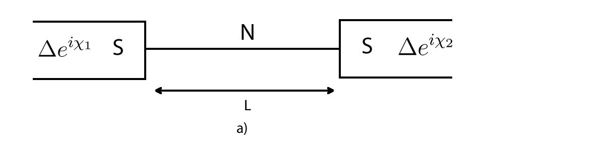
(a)

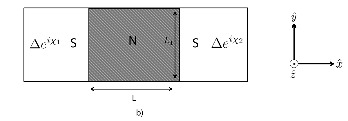
(b)

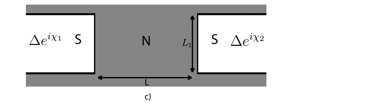
(c)

Figure 1: Qualitative representation of a) 1D SNS junction b) Bulk junction with closed boundaries c) Bulk junction with open boundaries.

The I-U characteristics of SNS junctions depend on the external circuits to which they are connected. In what follows, we will be interested in I-U characteristics of the junctions in situations where either the voltage (voltage bias setup) or current (current bias setup) is fixed by the external circuit. In Figs. 2, 3, and 4 we qualitatively summarize our results for the cases of voltage- and current-biased junctions.

In the case of voltage-biased junctions the I-U characteristic turns out to be non-monotonic, and the maximum current $J_{max}$ is reached at $eU\sim\tau_{in}^{-1}$ [12]. We will show that the value of $J_{max}$ can be significantly larger than the temperature-dependent critical current $J_{c}(T)$, and in some cases it can be as large as the zero temperature critical current $J_{c}(0)$. At even larger voltages the I-U characteristic reaches a minimum, after which the current increases with voltage.

In the case of current-biased junctions at $J_{c}<J<J_{jump}$ the voltage monotonically increases from zero to a relatively small value, which is inversely proportional to $\tau_{in}$. Then, at $J=J_{jump}\sim J_{max}$ the I-U characteristic exhibits a jump to a significantly higher voltage.

The presentation below is organized as follows. In Sec. 2 we obtain general expressions for the diagonal contribution to current in terms of the inelastic relaxation time $\tau_{in}$ and sensitivity of quasi-particle energy levels to the change in the phase difference across the junction. In Sec. 3 we discuss the characteristic features of the current-voltage characteristics of voltage and current-biased SNS junctions, which are caused by the presence of the long inelastic relaxation time, $\tau_{in}$ in the system. In Sec. 4 we apply the general formalism developed in Sec. 2 to study the I-U characteristics of ballistic single channel junctions (Sec. 4.1) and diffusive multi-channel junctions (Sec. 4.2). We present our conclusions in Sec. 5. Finally, in A we present a derivation of our general equations in Sec. 2 in the diffusive regime starting from the Larkin-Ovchinnikov equations for the quasi-classical Green’s functions.

2 Description of the dynamics of SNS junction in adiabatic approximation.

Due to Andreev reflection from the normal metal-superconductor boundaries of the SNS junction, low energy ($\epsilon<\Delta$) quasi-particles are trapped inside the normal region. If the voltage across the SNS junction is sufficiently small, the quasi-particle energies $\epsilon_{i}(\chi(t))$ can be calculated in the adiabatic approximation, treating the phase difference $\chi(t)$ as a parameter.

At finite temperature, the quasi-particles occupying these levels move in energy space together with the levels. This motion creates a non-equilibrium quasi-particle distribution, which relaxes via inelastic scattering and leads to dissipation. There are two equivalent ways to describe this non-equilibrium distribution. The first is to describe the occupancy of time-dependent energy levels. This description is similar to the Lagrangian description of fluid dynamics. The second approach is to consider the electron distribution as a function of energy, in analogy to the Eulerian description of fluid dynamics.

The Lagrangian description is convenient in the cases where individual quasi-particle energy levels are well resolved, and the Eulerian description is more suitable for systems where energy levels form a continuum. In order to obtain the kinetic description of non-equilibrium dynamics of the junctions it is easier to start with the Lagrangian description. The corresponding equations in the Eulerian approach are then obtained by a straightforward change of variables.

2.1 Lagrangian description of dynamics of SNS junctions.

Let us introduce the occupation number of $i_{th}$ level $n_{i}(t)$. In the adiabatic approximation only scattering can change the occupation of a particular level, so the time evolution of $n_{i}(t)$ is controlled by the following equation,

$$\frac{dn_{i}(t)}{dt}=I_{st}\{n_{i}\}.$$ (3)

We will use an expression for the scattering integral in the relaxation time approximation

$$I_{st}=\frac{n_{F}(\epsilon_{i}(t))-n_{i}(t)}{\tau_{in}},$$ (4)

where $n_{F}(\epsilon)=1/(1+\exp(\epsilon/T))$ is the Fermi distribution function, and we assume that the relaxation time $\tau_{in}(T)$ depends only on the temperature.

In general, the relaxation time approximation is valid with precision of order one. However, in some cases this approximation turns out to be asymptotically exact. In particular, this is the case when the normal part of the junction is in the diffusive limit and the temperature is larger than the Thouless energy. (See the corresponding discussion in Section (4.2)) At $t\gg\tau_{in}$ the general solution of Eqs. (3),(4) is given by

$$n_{i}(t)=\int^{\infty}_{0}\frac{d\tau}{\tau_{in}}e^{\frac{-\tau}{\tau_{i}}}n_{F}(\epsilon_{i}(t-\tau)).$$ (5)

The diagonal component of the current through the junction can be written as

$$J_{d}=2e\frac{\partial E}{\partial\chi}=J_{c}(0)Y(\chi,0)+2e\sum_{i}\frac{\partial\epsilon_{i}(\chi)}{\partial\chi}n_{i}.$$ (6)

The first term in Eq. (6) represents the super-current through the system in the ground state. Here $J_{c}(0)$ is the critical current at zero temperature, and $Y(\chi,0)$ is a periodic function with maximum $1$ and a period $2\pi$.

2.2 Eulerian description

In the Eulerian description the quasi-particle distribution function inside the normal region is a function of energy and time $n(\epsilon,t)$. This description is convenient in the case where the energy levels are broadened on the energy scale larger than the level spacing. The number of levels in the system is conserved, so the density of states is therefore subject to the continuity equation in energy space

$$\partial_{t}\nu(\epsilon,\chi)+\partial_{\epsilon}\big{(}v_{\nu}(\epsilon,\chi)\nu(\epsilon,\chi)\big{)}=0,$$ (7)

where $v_{\nu}(\epsilon,\chi)$ is the level “velocity” in energy space. Using Eqs. (1), (7) the level velocity can be expressed in the form

$$v_{\nu}(\epsilon,\chi)=2eU\cdot V_{\nu}(\epsilon,\chi),$$ (8)

where

$$V_{\nu}(\epsilon,\chi)=-\frac{1}{\nu(\epsilon,\chi)}\int_{0}^{\epsilon}d\tilde{\epsilon}\frac{\partial\nu(\tilde{\epsilon},\chi)}{\partial\chi}$$ (9)

characterizes the sensitivity of the energy levels to changes of $\chi(t)$. In the absence of inelastic scattering, the time evolution due to the spectral flow is described by the continuity equation $\partial_{t}(\nu n)+\partial_{\epsilon}(v_{\nu}\nu n)=0$. Combining it with Eq. (8) for $\nu(\epsilon,\chi)$ and allowing for inelastic collisions we obtain the kinetic equation

$$\partial_{t}n(\epsilon,t)+2eU(t)\cdot V_{\nu}(\epsilon,\chi)\,\partial_{\epsilon}n(\epsilon,t)=I_{\mathrm{in}}\{n\}.$$ (10)

The expression for the current in the Eulerian description has a form

$$J_{d}=J_{c}(0)Y(\chi,0)-2e\int_{0}^{\infty}d\epsilon\nu(\epsilon,t)n(\epsilon,t)V_{\nu}(\epsilon,\chi).$$ (11)

Introducing the integrated density of states

$$N(\epsilon,t)=\int^{\epsilon}_{0}d\epsilon\nu(\epsilon,t),$$ (12)

and changing the variables from $\epsilon$ to $N(\epsilon,t)$, we can write Eq. (10) as

$$\partial_{t}n(N,t)=\frac{n_{F}(\epsilon(N,t))-n(N,t)}{\tau_{in}}.$$ (13)

It has a general solution given by,

$$n(N,t)=\int^{\infty}_{0}\frac{d\tau}{\tau_{in}}e^{\frac{-\tau}{\tau_{in}}}n_{F}(\epsilon(N,t-\tau)).$$ (14)

Small voltage regime: The description of dissipative current presented above simplifies significantly for slow time-dependence of the phase difference, $\dot{\chi}(t)=2eU(t)\ll\tau_{in}^{-1}$. In this case, to first order accuracy in $U(t)$, the diagonal contribution to the current can be written in the form

$$J_{d}(t,T)=J_{c}(T)Y(\chi(t),T)+G_{d}[\chi(t)]U(t).$$ (15)

Here the first term represents the equilibrium super-current corresponding to the instantaneous value of $\chi(t)$. It is convenient to express it as a product of the temperature dependent critical current $J_{c}(T)$ and a dimensionless periodic function periodic function of $\chi$ of unit amplitude, $Y(\chi,T)$. For example, at large temperatures $Y(\chi,T)\sim\sin\chi$.

The second term in Eq. (15) describes the diagonal contribution of the dissipative current and is characterized by the “diagonal conductance” $G_{d}[\chi(t)]$, which depends on the instantaneous phase difference phase difference $\chi(t)$. It can be evaluated by solving Eqs. (3),  (4), and (10) to first order in $U(t)$, then substituting the result into equation Eqs. (6), (11). This yields the following expressions for the diagonal conductance in the Lagrangian and Eulerian variables

$$G_{d}[\chi] = -4e^{2}\tau_{in}\sum_{i}\partial_{\epsilon}n_{F}(\epsilon_{i})\big{(}\partial_{\chi}\epsilon_{i}(\chi)\big{)}^{2}$$ (16a)

$$= -4e^{2}\tau_{in}\int_{0}^{\infty}d\epsilon\nu(\epsilon,\chi)V^{2}_{\nu}(\epsilon,\chi)\partial_{\epsilon}n_{F}(\epsilon).$$ (16b)

Thus, at sufficiently small voltages the diagonal contribution to the current can be expressed in terms of the phase dependent density of states $\nu(\epsilon,\chi)$, and is proportional to the inelastic relaxation time $\tau_{in}$.

The non-diagonal contribution to the current corresponds to elastic electron transfer between the superconducting banks of the junction, and may be expressed as $J_{nd}=G_{nd}U(t)$. Since it is not proportional to $\tau_{in}$ we have $G_{nd}\ll G_{d}$. Therefore, at small voltages, it is possible to neglect $J_{nd}$ compared to $J_{d}$.

Equations (3)-(11) which describe slow dynamics of SNS junctions in terms of the $\chi$ and $\epsilon$ -dependence of the quasi-particle density of states $\nu(\epsilon,\chi)$ are quite general. They hold at relatively small voltages, where the spectrum of quasi-particles in the normal region of the junction can be calculated in the adiabatic approximation, and the quasi-particle distribution function inside the normal region is spatially uniform.

In A we present a derivation of Eqs. (9), (10), and (11) in the diffusive regime, $L\gg l$, using a procedure developed by Larkin-Ovchinnikov [13]. Here $l=v_{F}\tau_{el}$ is the elastic mean free path, $v_{F}$ is the Fermi velocity, and $L$ is the length of the junction (See Fig. 1).

3 General features of I-U characteristics of SNS junctions

The form of $\chi(t)$ in a junction depends on the external circuit. Below we consider the I-U characteristics for two common setups: voltage-biased junction, and current-biased junction.

We show that the existence of the long inelastic relaxation time $\tau_{in}$ has a dramatic effect on the shape of the I-U characteristics of the junctions. In the voltage bias case the I-U characteristic becomes non-monotonic: it acquires an $N$-shape, as illustrated in Fig. 2. In the current-bias case the voltage dependence on the applied current is illustrated in Fig. 4. Broadly speaking it consists of two regions: 1) At relatively small excess of the bias current over the critical current the time-averaged voltage across the junction monotonically increases from zero, while its value remains rather small (inversely proportional to the inelastic relaxation time), 2) At larger bias currents, $J\sim J_{jump}$, the voltage exhibits a sharp jump to a much higher value. This feature of the dependence of the voltage on the bias current may have important implications for the interpretation of experimental data; because of the low values of the voltage in region 1) the transition to region 2) may be mistaken for the transition from the dissipationless to the dissipative state of the junction. Below, we show that the shape of the I-U characteristics at low voltages can be described in terms of the phase-dependence of the quasi-particle density of states in the junction.

3.1 Voltage biased SNS junctions

In the voltage bias case we define the nonlinear conductance $\bar{G}(U)$ as

$$\bar{G}(U)=\frac{\langle J(t)\rangle}{U},$$ (17)

where $\langle\ldots\rangle$ denotes averaging over time. Since the phase winds at a constant rate via the Josephson relation Eq. (1), after averaging over time the non-dissipative component of the current vanishes. We focus on the regime of low bias voltages, where the dissipative component of the current is dominated by the diagonal contribution.

We choose here to work in Eularian variables. To obtain the expression for the nonlinear conductance in this regime we substitute Eqs. (6) and (5) into Eq. (17). It is convenient to change from integration over time $\tau$ in Eq. (5) to an integration over phase $\phi$,

$$n(N,t)= \frac{1}{2eU\tau_{in}}\int^{\infty}_{0}d\phi e^{-\phi/2eU\tau_{in}}n_{F}\big{[}\epsilon\big{(}N,\chi(t)-\phi\big{)}\big{]}.$$ (18)

When the temperature is large as compared to the typical range of motion of the quasi-particle energy levels, we can expand the Fermi function deviations of the instantaneous quasi-particle energies from their average positions $\langle\epsilon(N,\phi)\rangle_{\phi}$,

$$\delta\epsilon(N,\chi)\equiv \,\epsilon(N,\chi)-\langle\epsilon(N,\phi)\rangle_{\phi}.$$ (19)

This yields,

$$n\big{(}N,t\big{)}= \,n_{F}\big{[}\langle\epsilon(N,\phi)\rangle_{\phi}\big{]}$$

$$+\,\frac{\partial_{\epsilon}n_{F}[\langle\epsilon(N,\phi)\rangle_{\phi}\big{]}}{2eU\tau_{in}}\int^{\infty}_{0}d\phi\exp\left(-\frac{\phi}{2eU\tau_{in}}\right)\delta\epsilon(N,\chi(t)-\phi).$$ (20)

Expanding the periodic phase dependence of the energy of quasi-particle levels in a Fourier series,

$$\delta\epsilon\big{(}N,\chi)=\sum_{k\neq 0}C_{k}\big{(}N\big{)}e^{ik\chi},$$ (21)

and using Eqs. (3.1), (21) and the expression for the current Eq. (11), we obtain the following expression for the non-linear conductance

$$\begin{split}\bar{G}_{d}(U)=-4e^{2}\tau_{in}\int^{\infty}_{0}dN\partial_{\epsilon}n_{F}\big{[}\big{\langle}\epsilon\big{(}N,\chi\big{)}\big{\rangle}_{\chi}\big{]}\sum_{k\neq 0}\frac{k^{2}}{1+(2keU\tau_{in})^{2}}|C_{k}(N)|^{2}.\end{split}$$ (22)

At small voltages, $eU\ll\tau_{in}^{-1}$, we obtain the linear conductance,

$$\begin{split}\bar{G}_{d}(0)=-4e^{2}\tau_{in}\int^{\infty}_{0}dN\partial_{\epsilon}n_{F}\big{[}\big{\langle}\epsilon\big{(}N,\chi\big{)}\big{\rangle}_{\chi}\big{]}\sum_{k\neq 0}k^{2}|C_{k}(N)|^{2}.\end{split}$$ (23)

Comparing with Eq. (16a) we see that the linear conductance can be equivalently expressed in the terms of the phase dependent conductance $G_{d}[\chi]$ introduced in Eq. (15),

$$\bar{G}_{d}(0)=\int_{0}^{2\pi}\frac{d\chi}{2\pi}G_{d}[\chi].$$ (24)

At large voltages, $eU\gg\tau^{-1}_{in}$, Eq. (22) yields

$$\bar{G}_{d}(U)=-\frac{1}{U^{2}\tau_{in}}\int^{\infty}_{0}dN\partial_{\epsilon}n_{F}\big{[}\big{\langle}\epsilon\big{(}N,\chi\big{)}\big{\rangle}_{\chi}\big{]}\sum_{k\neq 0}|C_{k}(N)|^{2}.$$ (25)

For a typical phase-dependence of the quasi-particle spectrum, the Fourier sums in Eqs. (23) and (25) are dominated by $k$ of order unity. In this case, nonlinear conductance at $eU\gg\tau^{-1}_{in}$ can be estimated as

$$\bar{G}_{d}(U)\sim\frac{\bar{G}_{d}(0)}{(eU\tau_{in})^{2}}.$$ (26)

According to Eq. (26), at $eU\gg\tau^{-1}_{in}$ the dc current $\langle J\rangle=\bar{G}_{d}(U)U$ decreases as the voltage increases. Thus, $\langle J\rangle$ has a maximum at $eU\sim\tau^{-1}_{in}$. The maximal current,

$$J_{max}\sim\frac{\bar{G}_{d}(0)}{e\tau_{in}},$$ (27)

can be expressed in terms of the $\chi$-dependence of the quasi-particle spectrum using Eqs. (24) and (15). In the Lagrangian and Eulerian variables the corresponding expressions have the form

$$J_{max} \sim -4e\int d\chi\sum_{i}\partial_{\epsilon}n_{F}(\epsilon_{i})\big{(}\partial_{\chi}\epsilon_{i}(\chi(t))\big{)}^{2}$$ (28)

$$= -4e\int d\chi\int_{0}^{\infty}d\epsilon\nu(\epsilon,\chi)V^{2}_{\nu}(\epsilon,\chi)\partial_{\epsilon}n_{F}(\epsilon).$$

It is worth noting that, since at high temperatures the equilibrium critical current $J_{c}(T)$ is exponentially decaying function of $T$, the value of $J_{max}$ can be much larger $J_{c}(T)$, and in some cases it can be as large as critical super-current at zero temperature $J_{c}(0)$.

Equation (26) describing the decrease of the nonlinear conductance with increasing voltage applies as long as the non-diagonal contribution to the dissipative current $J_{nd}=G_{nd}U(t)$ can be neglected. At voltages

$$U\sim U_{min}\equiv\frac{1}{\tau_{in}}\bigg{[}\frac{\bar{G}_{d}(0)}{G_{nd}}\bigg{]}^{1/2}\gg\frac{1}{\tau_{in}},$$ (29)

the $I-U$ characteristic develops a minimum. At $U>U_{min}$ the dissipative current is dominated by the non-diagonal contribution $J_{nd}$, which increases with $U$. It has been studied in many articles, see for example Refs. [14, 15, 16, 17, 18, 19]. The shape of the $I-U$ characteristics of the junctions of voltage-biased junctions is illustrated in Fig. 2. A somewhat different mechanism of N-type I-U characteristics of weak link has been discussed in Refs.  [3, 12, 20].

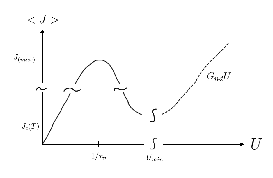
Figure 2: A schematic picture of an I-U characteristics of a voltage-biased SNS junction. The value of $J_{(max)}>J_{c}(T)$ can be significantly larger than the value of the equilibrium critical current of the junction $J_{c}(T)$.

3.2 I-U characteristics of current-biased junctions

In the current bias setup, the SNS junction undergoes a transition into a resistive state when the bias current $J$ exceeds the critical current $J_{c}(T)$. In this case the phase difference $\chi(t)$ increases monotonically, while the voltage $U(t)$ changes periodically with time, as illustrated in Fig. 3. In the following we will be interested in the dependence of the voltage averaged over the period of oscillations, $\langle U(t)\rangle$, on the bias current $J$. Qualitatively, the I-U characteristics of the current-biased SNS junctions is shown in Fig. 4. In a wide interval of bias currents $J>J_{c}(T)$ the average voltage on the junction is relatively small because it is inversely proportional to the the inelastic relaxation time $\tau_{in}$, which is the longest relaxation time in the system. At a higher bias current, $J\approx J_{jump}$, the voltage exhibits a relatively sharp jump to a much larger value. The magnitude of $J_{jump}$ turns out to be of the same order as the maximal current $J_{max}$ in the voltage-bias case, which is given by Eq. (28).

We will focus on the range of bias currents $J_{c}(T)<J<J_{jump}$, in which the current is dominated by the diagonal component $J_{d}$. It is important to note however that according to Eqs. (6) and (11), at the time-reversal invariant points $\chi=\pi n$, where $n$ is an integer, the sensitivity of all quasi-particle levels with respect to the phase change vanishes. As a result, $J_{d}$ vanishes at these points, and in some intervals near these points the bias current must be carried by the non-diagonal contribution, $J_{nd}$. Thus, the phase and time periods of the oscillations can be separated into two diagonal and two non-diagonal intervals, $t_{p}=(t_{d,1}+t_{d,2}+t_{nd,1}+t_{nd,2})$, and $2\pi=\chi_{d,1}+\chi_{nd,1}+\chi_{d,2}+\chi_{nd,2}$, in which the bias current is dominated by the diagonal, $J_{d}$, or non-diagonal, $J_{nd}$, contributions respectively. The relatively sharp distinction between these two intervals is possible because $\bar{G}_{d}(0)\gg G_{nd}$.

The boundaries of the non-diagonal intervals $\chi_{nd}$ can be determined from the condition that, at $\dot{\chi}\sim 1/\tau_{in}$ the bias current can be carried by the maximal diagonal contribution, $J_{d}\sim G_{d}(\chi)/e\tau_{in}=J$. In the vicinity of the time-reversal invariant points, $\chi=\pi n+\delta\chi$, we have

$$G_{d}(\chi)\sim\frac{\delta\chi^{2}}{2}\left.\frac{d^{2}G_{d}(\chi)}{d\chi^{2}}\right|_{\chi=\pi n}\sim\bar{G}_{d}(0)\frac{\delta\chi^{2}}{2}.$$ (30)

As a result, we get the following estimate for the width of the non-diagonal phase intervals: $\chi_{nd}\sim\sqrt{J/J_{jump}}$.

Inside the diagonal interval the phase winds at a rate of order of $eU_{d}=eJ/\bar{G}_{d}(0)$, whereas inside the non-diagonal interval it winds at a rate $eU_{nd}=eJ/G_{nd}$. Therefore we can neglect $t_{nd}\sim(G_{nd}/\bar{G}_{d}(0))(\chi_{nd}/\chi_{d})t_{d}\ll t_{d}$ in Eq. (31). Thus, using the Josephson relation (1), the average voltage can be expressed in terms of the duration of the diagonal time intervals only,

$$\langle U\rangle=\frac{\pi}{et_{p}}\approx\frac{\pi}{e\left(t_{d,1}+t_{d,2}\right)}.$$ (31)

If the instantaneous phase is not to close to the time-reversal invariant points, $\chi=n\pi$, the rate of change of phase is small, and the current may be expressed in terms of the instantaneous phase $\chi$ and its derivative via Eq. (15). Using this relation, the duration of the diagonal time intervals may be expressed as

$$t_{d,i}=\frac{1}{2e}\int_{\chi_{d,i}}\frac{G_{d}[\chi]d\chi}{J-J_{c}(T)Y(\chi,T)},$$ (32)

where $i=1,2$, and the integration is taken over the phase interval $\chi_{d,i}$.

At small excess current, $J-J_{c}(T)\ll J_{c}(T)$, we can expand $Y(\chi,T)$ near its maximum at $\chi=\chi_{m}$, while at $J>J_{c}$ we can neglect the second term in the denominator in Eq. (32). Then, using Eq. (31) we get

$$\langle U(J)\rangle=\begin{cases}\sqrt{2J_{c}(J-J_{c})}/G_{d}[\chi_{m}]&,J-J_{c}\ll J_{c},\\ \sim J/\bar{G}_{d}(0)&,J_{c}\ll J\ll J_{jump}.\end{cases}$$ (33)

According to Eqs. (16) and (33), at relatively small currents the voltage across the junction is smaller than $1/\tau_{in}$. This justifies the use of linear in $\dot{\chi}$ approximation for the dissipative part of the current through the junction.

Similarly to the case of voltage-based junction, in the current-biased case the diagonal component of the current $J_{d}$ has a maximum at $U\sim 1/e\tau_{in}$, which is of order of $J_{jump}$. When the bias current, $J$ reaches this value, the widths of the phase intervals $\chi_{d,i}$ shrinks to zero, and the voltage-current dependence $\langle U(J)\rangle$ jumps to the branch dominated by the non-diagonal contribution to the current $J_{nd}$.

Near $J=J_{jump}$ the non-diagonal interval covers nearly the entire phase interval from $0$ to $2\pi$, with the exception of points near $\chi_{max}^{(G)}$, where $G_{d}[\chi]$ reaches its maximum. Expanding $G_{d}[\chi]$ near its maximum, we estimate the conductance at the edge of the diagonal interval

$$G_{d}[\chi_{max}^{(G)}+\chi_{d}]\sim J_{jump}\tau_{in}-\bar{G}_{d}(0)\chi^{2}_{d}.$$ (34)

If the current is fixed at $J=J_{jump}-\delta J$, then the size of the diagonal interval is given by $\delta J\sim\bar{G}_{d}(0)\chi^{2}_{d}/\tau_{in}\sim J_{jump}\chi_{d}^{2}$. Within the width of the jump the diagonal and non-diagonal time intervals are of the same order $t_{nd}\sim t_{d}$, which means that $\chi_{d}\sim\bar{G}_{d}(0)/G_{nd}$. Therefore, we estimate the width of the jump to be,

$$\delta J\sim J_{jump}\bigg{(}\frac{G_{nd}}{\bar{G}_{d}(0)}\bigg{)}^{2}\ll J_{jump}.$$ (35)

In the regime $J>J_{jump}$ the voltage on the junction $U\sim J/G_{nd}\gg 1/\tau_{in}$, the diagonal contribution to the current $J_{d}$ is suppressed, and the I-U characteristics of the junctions are controlled by the non-diagonal contribution to the current, $J_{nd}=G_{nd}U$.

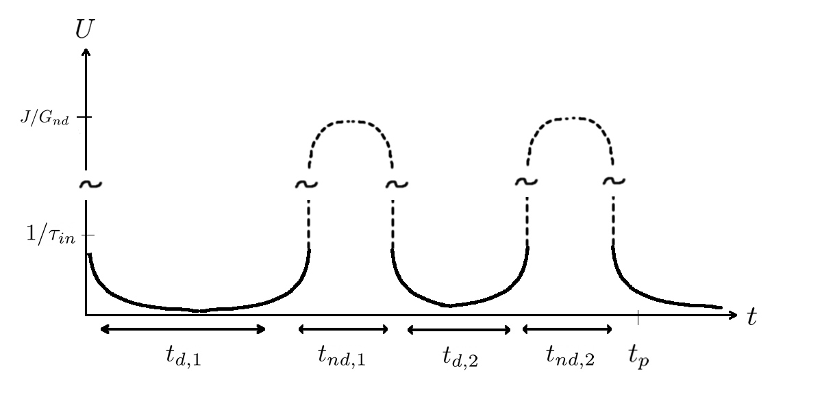
Figure 3: Time dependence of voltage at a current-based SNS junction when $J>J_{c}(T)$.

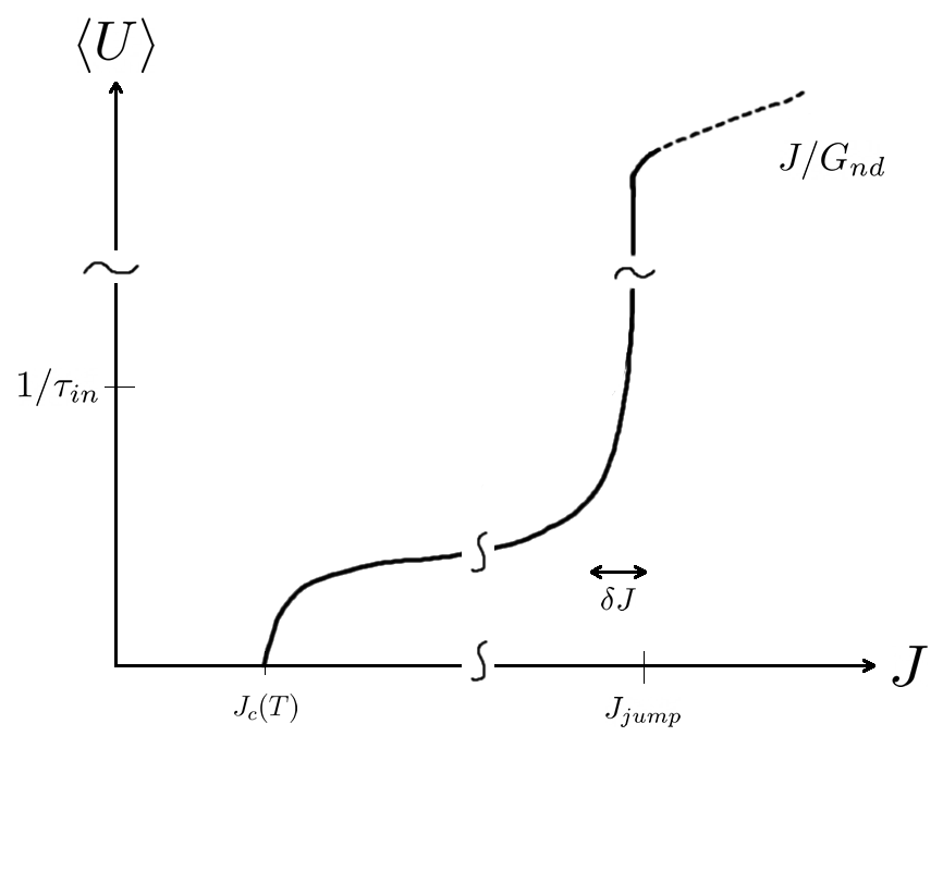
Figure 4: Schematic picture of the I-U characteristic of the current-based SNS junction.

4 I-U characteristics of SNS junctions in clean and diffusive regimes

As was shown in Sec. 3, the I-U characteristics of both voltage- and current- biased SNS junctions can be characterized by the parameter $\bar{G}_{d}(0)\sim G_{d}[\chi_{m}]$; see Eqs. (24), (26), and (33). In this section we will evaluate this parameter in the cases of ballistic single channel junctions, and diffusive multi-channel junctions.

4.1 Clean 1D SNS junction.

In this subsection we consider a junction, in which the normal region consists of a clean single channel metallic wire. We assume that the length of the wire $L$ is larger than the superconducting coherence length. In this case one can evaluate the quasi-particle spectrum by solving the stationary Bogoliubov-De Gennes equations in the normal metal at fixed value of $\chi$ with appropriate boundary conditions at NS boundaries (see for example Refs. [21] and [22] )

$$\begin{bmatrix}\frac{\hat{p}^{2}}{2m}-\mu&0\\ 0&-\frac{\hat{p}^{2}}{2m}+\mu\end{bmatrix}\begin{bmatrix}\psi_{e}\\ \psi_{h}\end{bmatrix}=\epsilon\begin{bmatrix}\psi_{e}\\ \psi_{h}\end{bmatrix}.$$ (36)

Below we assume that the transmission coefficients of both contacts are the same and equal to $r$. In the limiting cases of high and low transparency the spectrum for $\epsilon<\Delta$ is given by

$$\epsilon^{\pm}_{n}(\chi)=\frac{v_{F}}{L}\begin{cases}\pi(n+\frac{1}{2})\pm\frac{\chi}{2},&r=1,\\ n\pi\pm 2r\sqrt{2(1+\cos\chi)},&r\ll 1.\end{cases}$$ (37)

Here $n=0,1...$ is integer, $v_{F}$ is the Fermi velocity, and the phase $\chi$ is understood modulo $2\pi$.

Below we evaluate the linear conductance $\bar{G}_{d}(0)$ given by Eqs. (16a) and (24), which can then be used to determine the values of the maximal current in the voltage-biased set up, $J_{max}$ and the current at which the transition to a high resistance state occurs in the current- biased set up, $J_{jump}$, via Eq. (28).

Substituting Eq. (37) into Eq. (16a) we obtain an expression for the linear conductance at high temperatures

$$\bar{G}_{d}(0)=\frac{e^{2}}{\pi}\frac{v_{F}}{L}\tau_{in}A(r),\,\,\,\,\ T\gg v_{F}/L,$$ (38)

where

$$A(r)=\begin{cases}1&,r=1,\\ 8r^{2}&,r\ll 1.\end{cases}$$ (39)

We note that the conductance of a pure single channel SNS junction, Eq. (38), exceeds the normal state conductance $Ae^{2}/\hbar$, by a large factor $\frac{v_{F}}{L}\tau_{in}\gg 1$. Substituting Eq. (38) into Eq. (28), we get

$$J_{jump}\sim J_{max}\sim\frac{ev_{F}}{L}A(r).$$ (40)

The maximal current turns out to be temperature independent. The reason for this is that at low energies, $\epsilon_{n}\ll\Delta$, the sensitivity of the levels to a change in $\chi$ is independent of the energy.

It is instructive to compare value of $J_{max}$ and $J_{jump}$ in Eq. (40) with the critical current $J_{c}(T)$. The latter can be obtained by substituting Eq. (37), and the equilibrium Fermi distribution function $n_{F}(\epsilon_{i})$ into Eq. (6), see Ref. [21].

$$J_{c}(T)=B(r)\frac{ev_{F}}{2L}\begin{cases}1&,\quad T\ll\frac{v_{F}}{L},\\ \exp(-\frac{2\pi TL}{v_{F}})&,\quad T\gg\frac{v_{F}}{L}.\end{cases}$$ (41)

where the dimensionless coefficient $B(r)$ has the following limiting values at high and low contact transparencies,

$$B(r)=\begin{cases}1&,r=1,\\ r^{2}/2\pi&,r\ll 1.\end{cases}$$ (42)

Comparing Eqs. (40) and (41) we arrive to a somewhat surprising conclusion that at high temperatures, $T\gg v_{F}/L$, the values of $J_{max}$ and $J_{jump}$ are of order of the critical current at zero temperature,

$$J_{max}\sim J_{jump}\sim J_{c}(0)\gg J_{c}(T).$$ (43)

At small temperatures, $T\ll v_{F}/L$, the situation depends on the value of the transmission coefficient $r$. At $r=1$ the gap in the quasi-particle spectrum closes at $\chi=0,\pi$. In this case the main contribution to $\bar{G}_{d}(0)$ comes from the interval of times where the gap is of order $T$. In this case Eqs. (16), (24), (27) yield the same value for $\bar{G}$, $J_{jump}$, and $J_{max}$ as in Eqs. (38), (40).

If $r<1$, the gap in the spectrum does not close at any value of $\chi$. Therefore, at $T\ll v_{F}/L$ quasi-particle concentration inside the junction is exponentially low $n_{i}\sim\exp(-v_{F}/LT)$. In this case there are two relaxation times characterizing the dynamics of the system: relaxation time characterizing processes which conserve the total number of quasi-particles, $\tau_{in}$ , and the exponentially long recombination time ,$\tau_{in,r}\sim\tau_{in}\exp(v_{F}/LT)$, which characterizes the processes changing the total number of particle. The two exponential factors are canceled in Eq. (6) and we can estimate the low temperature linear conductance to be roughly the same order as in the high temperature case,

$$\bar{G}_{d}(U)\sim e^{2}\frac{v_{F}}{L}\tau_{in}\begin{cases}1&,(eU\tau_{in,r})\ll 1,\,\,\,\,\,\,\,r=1,\\ (eU\tau_{in,r})^{-2}&,(eU\tau_{in,r})\gg 1,\,\,\,\,\,\,\,r=1.\end{cases}$$ (44)

Note that since in this case $U_{max}\sim 1/e\tau_{in,r}\ll 1/\tau_{in}$, the value of the maximum current in the adiabatic regime turns out to be smaller than its value at high temperatures by an exponentially small factor $e^{-v_{F}/LT}$ . Accordingly, at small temperatures, $T\ll v_{F}/L$, we have $J_{max}\ll J_{c}(0)$.

4.2 Diffusive SNS junctions.

Let us now consider the case of a diffusive SNS junction shown in Fig. 1(b) , where two sides of a diffusive metal with the dimensions $L,L_{1},L_{2}\gg l=v_{F}\tau_{el}$ are attached to two superconducting parts of the junction, while the other two sides are in contact with insulator.

A general scheme of description of the kinetic phenomena in superconductors in the diffusive regime ($L\gg l$) has been developed by Larkin and Ovchinnikov [13]. It describes both diagonal $J_{d}$ and non-diagonal $J_{nd}$ parts of the current as long as $eU<\Delta$. In the appendix we review derivation Larkin-Ovchinnikov equations and show that at $eU<E_{T}$ they can be reduced to Eqs. (10) and (11). Here $E_{T}=\frac{D}{L^{2}}$ is the Thouless energy and $D=v_{F}^{2}\tau_{el}/3$ is the diffusion coefficient in the normal metal.

The density of states in the normal metal part of the junction can be written in terms of retarded Green’s function,

$$\nu(\epsilon,\chi)=\int_{V}d{\bf r}\tilde{\nu}(\epsilon,{\bf r},\chi)={2}\tilde{\nu}_{N}\mathrm{Re}\int_{V}d{\bf r}G_{0}^{R}(\epsilon,{\bf r},\chi).\color[rgb]{0,0,0}$$ (45)

Here the integral is taken over the normal metal region, $\tilde{\nu}({\bf r})$ is the local density of states in SNS junction, and $\tilde{\nu}_{N}$ is the density of states per unit volume per spin projection of the normal state, and $G_{0}^{R}(\epsilon,{\bf r},\chi)$ is the dimensionless semi-classical retarded Green’s function [13].

In the geometry of the SNS junction shown in Fig. 1b, $\tilde{\nu}$ depends only on the $x$ coordinate. Using the normalization condition for the normal and anomalous retarded Green’s functions (see Eq. (A39) in the appendix), we parameterize them as follows

$$G_{0}^{R}(\epsilon,x)=\cos\theta(\epsilon,x),\,\,\ F_{0}^{R}=e^{i\tilde{\chi}(\epsilon,x)}\sin\theta(\epsilon,x),\,\,\ F_{0}^{R+}=e^{-i\tilde{\chi}(\epsilon,x)}\sin\theta(\epsilon,x),$$ (46)

and

$$\nu(\epsilon,\chi)={2}\tilde{\nu}_{N}(L_{1}L_{2})\int^{\frac{L}{2}}_{-\frac{L}{2}}dx\mathrm{Re}\big{[}\cos\theta(\epsilon,x)\big{]}.$$ (47)

Here $\theta$ and $\chi$ are complex.

In the diffusive regime the dependence of $\theta$ and $\tilde{\nu}(\epsilon,\chi,{\bf r})$ on $x$ and the phase difference $\chi$ can be obtained by solving the Usadel equations [23] (see Eqs. (A37) and (A38) in the Appendix). In the normal region, where $\Delta({\bf r})=0$ they have the form

$$\frac{D}{2}\bigg{(}\partial^{2}_{x}\theta-\frac{1}{2}\sin(2\theta)\big{(}\partial_{x}\tilde{\chi}\big{)}^{2}\bigg{)}= -\epsilon\sin\theta,$$ (48)

$$\partial_{x}\big{(}\sin^{2}\theta\partial_{x}\tilde{\chi}\big{)}= \,0.$$ (49)

The boundary conditions for these equations at $\epsilon<\Delta$ and $r=1$ are (see Ref. [24])

$$\begin{split}\theta(\epsilon;x=0,L)=\frac{\pi}{2};\,\,\,\,\,\,\tilde{\chi}(\epsilon;x=0,L)=\pm\frac{\chi}{2}.\end{split}$$ (50)

For $r\ll 1$ the boundary conditions have a form

$$\begin{split}D\partial_{x}\theta|_{\epsilon;x=0,L}=\pm rv_{F}\big{(}\cos\theta\big{)}\cos(\tilde{\chi}\pm\frac{\chi}{2})|_{\epsilon;x=0,L},\\ D\sin\theta\partial_{x}\tilde{\chi}|_{\epsilon;x=0,L}=\pm rv_{F}\sin(\tilde{\chi}\pm\frac{\chi}{2})|_{\epsilon;x=0,L}.\end{split}$$ (51)

Solutions of Eqs. (48),(49) were investigated in several articles (see for example, Refs. [17] and [25]).

The density of states in the normal region of SNS junctions differs from that in the normal metal only at small energies of the order of mini-gap $E_{g}$. For our purposes we need only rough features of $\epsilon$ and $\chi$ dependencies of the density of states,

$$\nu(\epsilon,\chi)={2}v\tilde{\nu}_{N}\begin{cases}0&,\epsilon<E_{g}(\chi),\\ h(\epsilon,\chi)&,\epsilon-E_{g}(\chi)\sim E_{g}(\chi),\\ 1&,\epsilon-E_{g}(\chi)>>E_{g}(\chi).\end{cases}$$ (52)

where $h(\epsilon,\chi)$ is of order unity, and $v=LL_{1}L_{2}$ is the volume of the normal metal region. When the phase winds from $0$ to $2\pi$ the value of mini-gap changes on the order of

$$E_{g}(0)\sim E_{T}\begin{cases}1&,r>\frac{l}{L},\\ r\frac{L}{l}&,r<\frac{l}{L},\end{cases}$$ (53)

which implies that $\partial_{\chi}E_{g}(\chi)\sim E_{g}(0)$.

Substituting Eq. (52) into Eqs. (9),(16) and averaging the result over the period of oscillations we can estimate the conductance of the junction as follows

$$\bar{G}_{d}(0,T)\sim G^{\prime}_{N}\tau_{in}\begin{cases}\frac{E_{g}^{2}(0)}{T}&\,\,\,\ ,T>E_{g}(0),\,\,\,\,\ U\ll 1/\tau_{in},\\ T&\,\,\,\,\,,T<E_{g}(0),\,\,\,\,\ U\ll 1/\tau_{in},\\ \end{cases}$$ (54)

where $G^{\prime}_{N}=e^{2}E_{g}(0)\tilde{\nu}_{N}v$. The situation at large voltages, $eU\gg\tau_{in}^{-1}$, is similar to that described in Sec (4.1) for a clean one-dimensional SNS junction. Namely, the nonlinear conductance $\bar{G}_{d}(U)$ is reduced from its linear value, Eq. (54), by the factor $(2eU\tau_{in})^{-2}$. Thus, the I-U characteristics of a voltage-biased junction has a maximum at $eU\sim\tau_{in}^{-1}$. The magnitude of the maximal current can be estimated as

$$J_{max}\sim J_{c}(0)\begin{cases}\frac{E_{g}(0)}{T}&\,\,\,\ ,T>E_{g}(0),\\ \frac{T}{E_{g}(0)}&\,\,\,\,\,,T<E_{g}(0).\\ \end{cases}$$ (55)

Here $J_{c}(0)=\frac{1}{e}G^{\prime}_{N}E_{g}(0)$ is the critical current of a diffusive SNS junction at $T=0$. We note that the value of $J_{max}$ can be significantly larger than $J_{c}(T)$.

At even larger larger voltages the dominant contribution to the current comes from $J_{nd}$, which is an increasing function of voltage. Let us consider the case $T\gtrsim E_{g}$. In this regime the part of the resistance of the junction corresponding to $J_{nd}$ is, essentially, the resistance of the sequence of the tunneling barriers and the normal metal resistances. It has been considered in many articles [14, 15, 16, 17, 18], [26] and [27]. For example, if $r=1$ and $E_{g}(0)\sim E_{T}$, then the contribution to the current from the non-diagonal part is on the order of the current in the normal state $J=G_{N}U$, where $G_{N}=e^{2}E_{T}\tilde{\nu}_{N}v$ is the conductance of normal metal part of SNS junction (see Eqs. (A56), (A57) in the appendix). As a result, using Eq. (54), we get an estimate for

$$U_{min}\sim\frac{E_{T}}{(T\tau_{in})^{1/2}}\ll E_{T}.$$ (56)

5 Conclusions.

We have shown that the I-U characteristics of SNS junctions at low temperatures and low voltages can be expressed in terms of the energy and the phase dependence of the density of states $\nu(\epsilon,\chi)$. In this case, they are controlled by the inelastic quasi-particle relaxation time $\tau_{in}$. In contrast, at large bias voltages and currents the I-U characteristics are controlled by the elastic relaxation time $\tau_{el}$ . Qualitatively, our results are shown in Figs. 2 and 4.

An interesting aspect of the problem is that for current-biased junctions, the jump in the I-U characteristics from the low voltage to high voltage regime (see Fig. 4) occurs at the value of the current $J=J_{jump}$, which can be significantly larger then the value of the equilibrium critical current $J_{c}(T)$. Therefore, determination of the critical currents of SNS junctions may require measurements of I-U characteristics at relatively small voltages, $eU<1/\tau_{in}$.

The results presented above are valid in situations where the low energy quasi-particles are trapped inside the normal region of the junction, and the only channel of the quasi-particle relaxation is the inelastic energy relaxation. In a different geometry, where the normal region of the junction is open to the bulk normal metal, as shown in Fig. 1(c), there is another channel of the relaxation via diffusion of quasi-particles into the bulk of the normal metal. In this case one can obtain an estimate for the conductance of the system substituting in Eq. (54)

$$\tau_{in}\rightarrow min[\tau^{(*)},\tau_{in}]$$ (57)

where $\tau^{*}\sim L^{2}_{1}/D$ is the time of diffusion on the length $L_{1}$.

Finally, it should be mentioned that the only symmetry requirement for the density of state in the time reversal symmetrical system is $\nu(\epsilon,\chi,{\bf H})=\nu(\epsilon,-\chi,-{\bf H})$. Therefore, for example, in the case on non-centrosymmetric films in the parallel magnetic field $\nu(\epsilon,\chi,H)\neq\nu(\epsilon,\chi,-H)$ and $\nu(\epsilon,\chi,H)\neq\nu(\epsilon,-\chi,H)$. As a result, in general, the I-U characteristics of the SNS junctions are non-reciprocal: $|J(U)\neq|J(-U)|$, and $|J(H)\neq|J(-H)|$.

6 Acknowledgment

This work of was supported by the National Science Foundation Grant MRSEC DMR-1719797 and also in part by the Thouless Institute for Quantum Matter and the College of Arts and Sciences at the University of Washington. The work BZS was funded by the Gordon and Betty Moore Foundation’s EPiQS Initiative through Grant GBMF8686.

Appendix A Derivation of Eqs. (10), (11) using Larkin-Ovchinnikov approach in the diffusive regime, $L\gg l$.

We start with the Gorkov equations for the Green’s functions in Keldysh representation [28]. We will denote matrices in Nambu space with a hat, $\hat{A}$, and matrices in both Nambu and Keldysh space with a check, $\check{A}$. We have chosen units such that $\hbar=c=1$. The Green’s function is defined by the following equation,

$$\begin{split}\bigg{(}i\hat{\tau}_{3}\partial_{t_{1}}+\frac{1}{2m}\bigg{(}{\bf\nabla_{r_{1}}}-ie\hat{\tau}_{3}{\bf A}({\bf r_{1}},t_{1})\bigg{)}^{2}+\mu\\ +\hat{\Delta}({\bf r_{1}},t_{1})-e\phi({\bf r_{1}},t_{1})\bigg{)}\check{G}({\bf r_{1}},{\bf r_{2}},t_{1},t_{2})\\ -(\check{\Sigma}\otimes\check{G})({\bf r_{1}},{\bf r_{2}},t_{1},t_{2})=\delta(\boldsymbol{r}_{1}-\boldsymbol{r}_{2})\delta(t_{1}-t_{2}).\end{split}$$ (A1)

Here ${\bf A}({\bf r},t)$ is the vector potential, $\hat{\Delta}({\bf r},t)$ is the superconducting order parameter, $\mu$ is the chemical potential, and $\phi({\bf r})$ is the scalar potential,

$$\check{G}=\begin{pmatrix}\hat{G}^{R}&\hat{G}^{K}\\ 0&\hat{G}^{A}\end{pmatrix}, \check{\Sigma}=\begin{pmatrix}\hat{\Sigma}^{R}&\hat{\Sigma}^{K}\\ 0&\hat{\Sigma}^{A}\end{pmatrix},$$ (A2)

where $\hat{G}^{R,A,K}$ are retarded, advanced, and Keldysh Green’s functions, and $\check{\Sigma}$ is the self energy. The cross operator in Eq. (A1) represents a convolution,

$$(O_{1}\otimes O_{2})({\bf r_{1}},{\bf r_{2}},t_{1},t_{2})=\int d{\bf r}\int dtO_{1}({\bf r_{1}},{\bf r},t_{1},t)O_{2}({\bf r},{\bf r_{2}},t,t_{2}).$$ (A3)

The conjugate equation to Eq. (A1) is given by

$$\begin{split}\check{G}({\bf r_{1}},{\bf r_{2}},t_{1},t_{2})\bigg{(}-i\hat{\tau}_{3}\partial_{t_{2}}+\frac{1}{2m}\bigg{(}{\bf\nabla_{r_{2}}}+ie\hat{\tau}_{3}{\bf A}({\bf r_{2}},t_{2})\bigg{)}^{2}+\\ \mu+\hat{\Delta}({\bf r_{2}},t_{2})-e\phi({\bf r_{2}},t_{2})\bigg{)}\\ -(\check{G}\otimes\check{\Sigma})({\bf r_{1}},{\bf r_{2}},t_{1},t_{2})=\delta(\boldsymbol{r}_{1}-\boldsymbol{r}_{2})\delta(t_{1}-t_{2}),\end{split}$$ (A4)

where the derivatives are understood to be acting towards the left. These equations should be supplemented with the self-consistent equation for the order parameter

$$\Delta(r,t)=\lambda F(r,t),$$ (A5)

where $\lambda$ is the electron interaction constant.

A.1 Quasi-classical approximation for the Gorkov equations.

Subtracting Eq. (A4) from Eq. (A1) gives the following equation for the Green’s functions,

$$\begin{split}i\hat{\tau}_{3}\partial_{t_{1}}\check{G}({\bf r_{1}},{\bf r_{2}},t_{1},t_{2})+i\hat{\partial}_{t_{2}}\check{G}({\bf r_{1}},{\bf r_{2}},t_{1},t_{2})\hat{\tau}_{3}\\ +\bigg{(}\frac{1}{2m}\bigg{(}{\bf\nabla_{r_{1}}}-ie{\bf A}({\bf r_{1}},t_{1})\bigg{)}^{2}+\mu+\hat{\Delta}({\bf r_{1}},t_{1})-e\phi({\bf r_{1}},t_{1})\bigg{)}\check{G}({\bf r_{1}},{\bf r_{2}},t_{1},t_{2})\\ -\check{G}({\bf r_{1}},{\bf r_{2}},t_{1},t_{2})\bigg{(}\frac{1}{2m}({\bf\nabla_{r_{2}}}+ie\hat{\tau}_{3}{\bf A}({\bf r_{2}},t_{2}))^{2}+\mu+\hat{\Delta}({\bf r_{2}},t_{2})-e\phi({\bf r_{2}},t_{2})\bigg{)}\\ =(\check{\Sigma}\otimes\check{G})({\bf r_{1}},{\bf r_{2}},t_{1},t_{2})-(\check{G}\otimes\check{\Sigma})({\bf r_{1}},{\bf r_{2}},t_{1},t_{2}).\end{split}$$ (A6)

In the limit where fields are slowly varying in space and time, we can use the quasi-classical approximation. Introducing the Wigner coordinates,

$$\begin{aligned} \boldsymbol{r}=\frac{1}{2}(\boldsymbol{r}_{1}+\boldsymbol{r}_{2}),&&\boldsymbol{\tilde{r}}=\boldsymbol{r}_{1}-\boldsymbol{r}_{2},\\ t=\frac{1}{2}(t_{1}+t_{2}),&&\tilde{t}=t_{1}-t_{2},\end{aligned}$$ (A7)

Fourier transforming equation Eq. (A6) over the relative position ${\bf\tilde{r}}$ as well as the relative time $\tilde{t}$, and dropping terms which are second order in derivatives, we arrive at the following equation

$$\begin{split}\frac{1}{2}\partial_{t}\big{\{}\hat{\tau}_{3},\check{G}(\epsilon,{\bf r},t,{\bf p})\big{\}}-i\epsilon\big{[}\hat{\tau}_{3},\check{G}(\epsilon,{\bf r},t,{\bf p})\big{]}+\frac{{\bf p}}{m}\cdot{\bf\nabla_{r}}\check{G}(\epsilon,{\bf r},{\bf p})\\ +\big{[}\hat{H}({\bf r},t,{\bf p}),\check{G}(\epsilon,{\bf r},t,{\bf p})\big{]}-\frac{i}{2}\big{\{}\partial_{t}\hat{H}({\bf r},t,{\bf p}),\partial_{\epsilon}\check{G}(\epsilon,{\bf r},t,{\bf p})\big{\}}\\ -\frac{e}{2m}{\bf A}({\bf r},t)\cdot{\bf\nabla_{r}}\big{\{}\hat{\tau}_{3},\check{G}(\epsilon,{\bf r},t,{\bf p})\big{\}}+\frac{i}{2}\big{\{}{\bf\nabla_{r}}\hat{H}({\bf r},t,{\bf p}),{\bf\nabla_{p}}\check{G}(\epsilon,{\bf r},t,{\bf p})\big{\}}\\ =-i\big{[}\check{\Sigma}(\epsilon,{\bf r},t,{\bf p}),\check{G}(\epsilon,{\bf r},t,{\bf p})\big{]}\\ +\frac{1}{2}\big{\{}{\bf\nabla_{r}}\check{\Sigma}(\epsilon,{\bf r},t,{\bf p}),{\bf\nabla_{p}}\check{G}(\epsilon,{\bf r},t,{\bf p})\big{\}}-\frac{1}{2}\big{\{}{\bf\nabla_{p}}\check{\Sigma}(\epsilon,{\bf r},t,{\bf p}),{\bf\nabla_{r}}\check{G}(\epsilon,{\bf r},t,{\bf p})\big{\}}\\ -\frac{1}{2}\big{\{}\partial_{t}\check{\Sigma}(\epsilon,{\bf r},t,{\bf p}),\partial_{\epsilon}\check{G}(\epsilon,{\bf r},t,{\bf p})\big{\}}+\frac{1}{2}\big{\{}\partial_{\epsilon}\check{\Sigma}(\epsilon,{\bf r},t,{\bf p}),\partial_{t}\check{G}(\epsilon,{\bf r},t,{\bf p})\big{\}}.\end{split}$$ (A8)

Here the brackets $[\cdot,\cdot]$ and $\{\cdot,\cdot\}$ stand for commutators and anti-commutators, and we have defined,

$$\check{G}(\epsilon,{\bf r},t,{\bf p})=\int dt\int d^{3}{\bf r}\check{G}({\bf r_{1}},{\bf r_{2}},t_{1},t_{2})e^{-i{\bf p}\cdot{\bf\tilde{r}}+i\epsilon\tilde{t}},$$ (A9)

$$\hat{H}({\bf r},t,{\bf p})=\frac{-ie}{m}{\bf A}({\bf r},t)\cdot{\bf p}\hat{\tau}_{3}-i\hat{\Delta}({\bf r},t)+\frac{ie^{2}}{m}{\bf A}^{2}({\bf r},t)+ie\phi({\bf r},t).$$ (A10)

A.2 The diffusion approximation for Gorkov equations.

The self-energy $\check{\Sigma}=\check{\Sigma}_{el}+\check{\Sigma}_{in}$ is a sum of two contributions corresponding to elastic and inelastic scattering respectively. In the case when the total scattering rate $\check{\Sigma}$ is smaller than the characteristic quasi-particle energy, it can be dropped from the equation for the retarded Green’s function. In this case the quasi-particle momentum is a good quantum number, and one can use a conventional Boltzmann kinetic equation for quasi-particle distribution function to describe slow superconducting dynamics [29]. In this article we will be interested in the opposite limit, where the quasi-particle momentum is not a good quantum number, and

$$\tau_{el}^{-1}>E_{T}>\tau_{in}^{-1}.$$ (A11)

We note that the Thouless energy, $E_{T}$ is a characteristic quasi-particle energy relevant to the problem. In this case $\check{\Sigma}_{in}$ still can be dropped from the equation for the retarded Green’s function, however $\check{\Sigma}_{el}$ is the largest term in Eq. (A8), and can not be neglected.

An effective approach to describe the quasi-particle dynamics in this limit was developed in Ref.[13]. This method is based on the fact that the elastic part of the self-energy can be expressed in terms of the Green’s functions,

$$\check{\Sigma}_{el}(\epsilon,{\bf r},t)=\frac{-1}{2\pi\tau_{el}}\int d^{3}{\bf p}\check{G}(\epsilon,{\bf r},t,{\bf p}),$$ (A12)

and thus $\check{\Sigma}_{el}$ does not depend on ${\bf p}$.

Let us integrate Eq. (A8) over $\xi_{p}=\frac{{\bf p}^{2}}{2m}-\mu$ for a fixed momentum direction $\bm{n}=\bm{p}/p$. On length scales larger then the Fermi wave length $p_{F}^{-1}$, to leading order in spacial gradients we get

$$\begin{split}\frac{1}{2}\partial_{t}\big{\{}\hat{\tau}_{3},\check{g}(\epsilon,{\bf r},t,{\bf n})\big{\}}-i\epsilon\big{[}\hat{\tau}_{3},\check{g}(\epsilon,{\bf r},t,{\bf n})\big{]}+v_{F}{\bf n}\cdot{\bf\nabla_{r}}\check{g}(\epsilon,{\bf r},{\bf n})\\ +\big{[}\hat{H}({\bf r},t,p_{F}{\bf n}),\check{g}(\epsilon,{\bf r},t,{\bf n})\big{]}-\frac{i}{2}\big{\{}\partial_{t}\hat{H}({\bf r},t,p_{F}{\bf n}),\partial_{\epsilon}\check{g}(\epsilon,{\bf r},t,{\bf n})\big{\}}\\ =-i\big{[}\check{\Sigma}_{el}(\epsilon,{\bf r},t),\check{g}(\epsilon,{\bf r},t,{\bf n})\big{]}-i\big{[}\check{\Sigma}_{in}(\epsilon,{\bf r},t),\check{g}(\epsilon,{\bf r},t,{\bf n})\big{]},\end{split}$$ (A13)

where we have defined

$$\check{g}(\epsilon,{\bf r},t,{\bf n})=\frac{i}{\pi}\int d\xi_{p}\check{G}(\epsilon,{\bf r},t,{\bf p}).$$ (A14)

We have introduced the factor $i/\pi$ to have the same notation as in Ref. [13].

Taking into account the normalization condition(see for example [30]),

$$(\check{g}\otimes\check{g})({\bf r},t_{1},t_{2},\boldsymbol{n})=\delta(t_{1}-t_{2}),$$ (A15)

we can parameterize the Keldysh component of $\check{g}$ as,

$$\hat{g}^{K}(t_{1},t_{2},\boldsymbol{n})=(\hat{g}^{R}\otimes\hat{f})(r,t_{1},t_{2},\boldsymbol{n})-(\hat{f}\otimes\hat{g}^{A})(r,t_{1},t_{2},\boldsymbol{n}).$$ (A16)

Since the matrix in the Nambu space $\hat{f}(r,t_{1},t_{2},{\bf n})$ has no off-diagonal component, we can expand it as

$$\hat{f}({\bf r},t_{1},t_{2},\boldsymbol{n})=f({\bf r},t_{1},t_{2},\boldsymbol{n})+\hat{\tau}_{3}f_{1}({\bf r},t_{1},t_{2},\boldsymbol{n}).$$ (A17)

To obtain $\hat{g}^{K}(\epsilon,{\bf r},t,{\bf n})$, we must Fourier transform Eq. (A16) with respect to the relative time difference. To zeroth order in time derivatives, we have

$$\hat{g}^{K}(\epsilon,{\bf r},t,{\bf n})=\hat{g}^{R}(\epsilon,{\bf r},t,{\bf n})\hat{f}(\epsilon,{\bf r},t,{\bf n})-\hat{f}(\epsilon,{\bf r},t,{\bf n})\hat{g}^{A}(\epsilon,{\bf r},t,{\bf n}).$$ (A18)

We can write $\hat{g}^{K}$ in the form,

$$\hat{g}^{K}(\epsilon,{\bf r},t,{\bf n})=2f(\epsilon,{\bf r},t,{\bf n})\hat{\delta}(\epsilon,{\bf r},t,{\bf n})+2f_{1}(\epsilon,{\bf r},t,{\bf n})\hat{\alpha}(\epsilon,{\bf r},t,{\bf n}),$$ (A19)

where we have defined,

$$2\hat{\alpha}(\epsilon,{\bf r},{\bf n})=\hat{g}^{R}(\epsilon,{\bf r},{\bf n})\hat{\tau}_{3}-\hat{\tau}_{3}\hat{g}^{A}(\epsilon,{\bf r},{\bf n}),$$ (A20)

$$2\hat{\delta}(\epsilon,{\bf r},{\bf n})=\hat{g}^{R}(\epsilon,{\bf r},{\bf n})-\hat{g}^{A}(\epsilon,{\bf r},{\bf n}).$$ (A21)

In the diffusive limit, where $\tau_{el}^{-1}$ is much larger than the typical energy scales of the problem, Greens functions are almost isotropic, and we can expand them in the spherical harmonics.

$$\check{g}(\epsilon,{\bf r},t,{\bf n})=\check{g}_{0}(\epsilon,{\bf r},t)+\check{\bf g_{1}}(\epsilon,{\bf r},t)\cdot{\bf n},\,\,\,\,\,\,\,\,\,\,\,\,\,\check{g}_{0}(\boldsymbol{r},t_{1},t_{2})\gg\check{\bf g}_{1}(\boldsymbol{r},t_{1},t_{2})\cdot\boldsymbol{n}.$$ (A22)

It follows from the normalization condition Eq. (A15), that

$$\check{g}_{0}(\epsilon,{\bf r},t)\check{g}_{0}(\epsilon,{\bf r},t)=1,\,\,\,\,\,\,\,\,\,\,\,\,\,\ \check{\bf g_{1}}(\epsilon,{\bf r},t)\check{g}_{0}(\epsilon,{\bf r},t)=-\check{g}_{0}(\epsilon,{\bf r},t)\check{\bf g_{1}}(\epsilon,{\bf r},t).$$ (A23)

Substituting Eq. (A22) into (A13), using Eq. (A23) and the fact that $\check{\Sigma}_{el}=\frac{-i}{2\tau_{el}}\check{g}_{0}$, in the linear in spacial gradients approximation we get

$$\check{\bf g_{1}}(\epsilon,{\bf r},t)= -\frac{3D}{v_{F}}\bigg{(}\check{g}_{0}(\epsilon,{\bf r},t){\boldsymbol{\partial}_{\bf r}}\check{g}_{0}(\epsilon,{\bf r},t)$$ (A24)

$$\,+\frac{e}{2}\partial_{t}{\bf A}({\bf r},t)\check{g}_{0}(\epsilon,{\bf r},t)\big{\{}\hat{\tau}_{3},\partial_{\epsilon}\check{g}_{0}(\epsilon,{\bf r},t)\big{\}}\bigg{)}.$$

Here $\boldsymbol{\partial}_{\bf r}={\bf\nabla_{r}}-ie{\bf A}({\bf r},t)[\hat{\tau}_{3},\cdot]$ is the covariant derivative. Substituting Eqs. (A22), (A24) into (A13), and averaging the result over direction of ${\bf n}$, we get an equation for the isotropic part of the Green’s functions $\check{g}_{0}$,

$$\begin{split}\frac{1}{2}\partial_{t}\big{\{}\hat{\tau}_{3},\check{g}_{0}(\epsilon,{\bf r},t)\big{\}}-i\epsilon\big{[}\hat{\tau}_{3},\check{g}_{0}(\epsilon,{\bf r},t)\big{]}-D{\boldsymbol{\partial}_{\bf r}}\cdot\bigg{(}\check{g}_{0}(\epsilon,{\bf r},t){\boldsymbol{\partial}_{\bf r}}\check{g}_{0}(\epsilon,{\bf r},t)\bigg{)}\\ +\frac{eD}{2}\partial_{t}{\bf A}({\bf r},t)\partial_{\epsilon}\big{\{}\hat{\tau}_{3},\check{g}_{0}(\epsilon,{\bf r},t){\boldsymbol{\partial}_{\bf r}}\check{g}_{0}(\epsilon,{\bf r},t)\big{\}}-i\big{[}\hat{\Delta}({\bf r},t),\check{g}_{0}(\epsilon,{\bf r},t)]\\ -\frac{1}{2}\big{\{}\partial_{t}\hat{\Delta}({\bf r},t),\partial_{\epsilon}\check{g}_{0}(\epsilon,{\bf r},t)\big{\}}+\partial_{t}\phi({\bf r},t)\partial_{\epsilon}\check{g}_{0}(\epsilon,{\bf r},t)\\ =-i\big{[}\check{\Sigma}_{in}(\epsilon,{\bf r},t),\check{g}_{0}(\epsilon,{\bf r},t)\big{]}.\end{split}$$ (A25)

In the adiabatic approximation, valid when the external perturbations vary slowly compared to $\Delta^{-1}$ , time derivatives can be dropped in the diagonal components of Eq. (A25) and we get Usadel’s equations [23] in matrix form

$$\begin{split}i\epsilon\big{[}\hat{\tau}_{3},\hat{g}^{R}_{0}(\epsilon,{\bf r},t)\big{]}+D{\boldsymbol{\partial}_{\bf r}}\cdot\bigg{(}\hat{g}^{R}_{0}(\epsilon,{\bf r},t)\boldsymbol{\partial}_{\bf r}\hat{g}^{R}_{0}(\epsilon,{\bf r},t)\bigg{)}\\ +i\big{[}\hat{\Delta}({\bf r},t),\hat{g}^{R}_{0}(\epsilon,{\bf r},t)\big{]}=0.\end{split}$$ (A26)

To get the two equations $f$ and $f_{1}$, we look at the Keldysh component of Eq. (A25) and take the trace in Nambu space (multiplying by a factor of $\hat{\tau}_{3}$ before taking the trace to get the second equation). As a result we have,

$$\begin{split}\tilde{\nu}(\epsilon,{\bf r},t)\partial_{t}f(\epsilon,{\bf r},t)+\frac{1}{4}eD\tilde{\nu}_{N}\partial_{\epsilon}f(\epsilon,{\bf r},t)\bigg{(}\partial_{t}{\bf A}({\bf r},t)\cdot{\bf j_{\epsilon}}({\bf r},t)\\ -2\mathrm{Tr}\big{\{}\partial_{t}\hat{\Delta}({\bf r},t)\hat{\delta}(\epsilon,{\bf r},t)\big{\}}\bigg{)}-\frac{1}{4}D\tilde{\nu}_{N}{\bf\nabla_{r}}\cdot\big{(}\Pi_{1}(\epsilon,{\bf r},t){\bf\nabla_{r}}f(\epsilon,{\bf r},t)\big{)}\\ -\frac{1}{4}D\tilde{\nu}_{N}{\bf\nabla_{r}}\cdot\big{(}f_{1}(\epsilon,{\bf r},t){\bf j_{\epsilon}}({\bf r},t)\big{)}=I_{1}\{f\},\end{split}$$ (A27)

$$\begin{split}\partial_{t}\big{(}f_{1}(\epsilon,{\bf r},t)\tilde{\nu}(\epsilon,{\bf r},t)\big{)}-\frac{1}{4}D\tilde{\nu}_{N}{\bf\nabla_{r}}\cdot\big{(}\Pi_{2}(\epsilon,{\bf r},t){\bf\nabla_{r}}f_{1}(\epsilon,{\bf r},t)\big{)}\\ -D\tilde{\nu}_{N}{\bf\nabla_{r}}\cdot\big{(}f(\epsilon,{\bf r},t)j_{\epsilon}({\bf r},t)\big{)}-\frac{i}{2}f_{1}(\epsilon,{\bf r},t)\mathrm{Tr}\big{\{}\big{(}g^{R}(\epsilon,{\bf r},t)\\ +g^{A}(\epsilon,{\bf r},t)\big{)}\hat{\Delta}(\epsilon,{\bf r},t)\big{\}}+\frac{1}{2}\partial_{\epsilon}f(\epsilon,{\bf r},t)\mathrm{Tr}\big{\{}e\partial_{t}\phi\hat{\alpha}(\epsilon,{\bf r},t)-\\ \partial_{t}\hat{\Delta}(\epsilon,{\bf r},t)\big{\}}=I_{2}\{f_{1}\}.\end{split}$$ (A28)

Here $\mathrm{Tr}$ stands for a trace in the Nambu space, and we have defined,

$$\Pi_{1}(\epsilon,{\bf r},t)=\mathrm{Tr}\{1-\hat{g}^{A}_{0}\hat{g}^{R}_{0}\},$$ (A29)

$$\Pi_{2}(\epsilon,{\bf r},t)=\mathrm{Tr}\{1-\hat{\tau}_{3}\hat{g}^{A}_{0}\hat{\tau}_{3}\hat{g}^{R}_{0}\},$$ (A30)

$${\bf j_{\epsilon}}=\mathrm{Tr}\big{\{}\hat{\tau}_{3}\big{(}\hat{g}^{R}_{0}{\boldsymbol{\partial}_{\bf r}}\hat{g}^{R}_{0}-\hat{g}^{A}_{0}{\boldsymbol{\partial}_{\bf r}}\hat{g}^{A}_{0}\big{)}\big{\}}.$$ (A31)

Since $\tau_{in}^{-1}\ll E_{T}$ the scattering integrals $I$ and $I_{1}$ have a standard form (see Refs. [13] and [29]) which can be obtained by substituting Eq. (A19) into the corresponding expression for $\Sigma_{in}$. They vanish when $f(\epsilon)=\tanh(\epsilon/2T)$ and $f_{1}=0$.

The current density can be expressed in terms of the Keldysh Green’s function,

$${\bf j}({\bf r,t})=-\frac{e\tilde{\nu}_{N}v_{F}}{4}\int^{\infty}_{-\infty}d\epsilon\int\frac{d\Omega_{n}}{4\pi}\mathrm{Tr}\big{\{}\hat{\tau}_{3}\hat{g}^{K}(\epsilon,{\bf r},t,{\bf n})\big{\}}{\bf n},$$ (A32)

where $\int\frac{d\Omega_{n}}{4\pi}$ indicates an integration over the direction of the momentum. Substituting the Keldysh component of Eq. (A24) into Eq. (A32) we get an expression for the current density ${\bf j}={\bf j_{d}}+{\bf j_{nd}}$, where ${\bf j_{d}}$ and ${\bf j_{nd}}$ are given by,

$${\bf j_{d}}({\bf r},t)=\frac{eD\tilde{\nu}_{N}}{4}\int^{\infty}_{-\infty}d\epsilon{\bf j_{\epsilon}}({\bf r},t)f(\epsilon,{\bf r},t),$$ (A33)

$$\begin{split}{\bf j_{nd}}({\bf r},t)=\frac{e\tilde{\nu}_{N}D}{8}\partial_{t}{\bf A}({\bf r},t)\int^{\infty}_{-\infty}d\epsilon\bigg{(}\Pi_{2}(\epsilon,{\bf r},t){\bf\nabla_{r}}f_{1}(\epsilon,{\bf r},t)+\\ \mathrm{Tr}\bigg{\{}2f_{1}\hat{\tau}_{3}(\hat{g}^{R}_{0}\partial_{\epsilon}\hat{g}^{R}_{0}-\hat{g}^{A}_{0}\partial_{\epsilon}\hat{g}^{A}_{0})+\partial_{\epsilon}f(1-\hat{g}^{R}_{0}\hat{g}^{A}_{0})\\ +\partial_{\epsilon}f_{1}(1-\hat{\tau}_{3}\hat{g}^{R}_{0}\hat{\tau}_{3}\hat{g}^{A}_{0})+f\hat{\tau}_{3}(\hat{g}^{R}_{0}\hat{\tau}_{3}\partial_{\epsilon}g^{R}_{0}-g^{A}_{0}\hat{\tau}_{3}\partial_{\epsilon}g^{A}_{0})\\ +\partial_{\epsilon}f\hat{\tau}_{3}(g^{R}_{0}\hat{\tau}_{3}g^{R}_{0}-\hat{g}^{R}_{0}\hat{\tau}_{3}\hat{g}^{A}_{0})+\partial_{\epsilon}f_{1}\hat{\tau}_{3}(1-g_{0}^{R}g_{0}^{A})\bigg{\}}\bigg{)}.\\ \end{split}$$ (A34)

The current conservation equation,

$${\bf\nabla_{r}}\cdot{\bf j_{\epsilon}}({\bf r},t)=0,$$ (A35)

can also be derived by multiplying Eq. (A26) by $\hat{\tau}_{3}$ and taking the trace in Nambu space.

In summary, we have derived a set of equations which describe the kinetics of superconductors in the diffusive regime. The density of states is determined by Usadel’s equation (A26), the distribution functions are determined by (A27) and (A28), and the expression for the current is given by (A33) and (A34).

A.3 Application of the general scheme to the case of SNS Junctions.

We consider the case where the interaction constant, and consequently the value of the order parameter inside the normal region of the SNS junction is zero. In this case we can use the following parametrization for the Green’s functions,

$$\hat{g}^{R}_{0}=\begin{pmatrix}G_{0}^{R}&F^{R}_{0}\\ -F^{R+}_{0}&-G_{0}^{R}\end{pmatrix}.$$ (A36)

Taking into account that the order parameter inside the normal metal region is zero, we get from Eqs. (A23),(A26) Usadel’s equations in the form

$${\bf\nabla_{\bf r}}\cdot\bigg{(}G^{R}_{0}{\bf\nabla_{\bf r}}G_{0}^{R}-F_{0}^{R}({\bf\nabla_{r}}+2ie{\bf A})F^{R+}_{0}\bigg{)}=0,$$ (A37)

$$i\epsilon F^{R}_{0}+\frac{D}{2}\bigg{(}{\bf\nabla_{r}}-2ie{\bf A}\bigg{)}\cdot\bigg{(}G_{0}^{R}({\bf\nabla_{r}}-2ie{\bf A})F^{R}_{0}-F^{R}_{0}{\bf\nabla_{r}}G^{R}_{0}\bigg{)}=0,$$ (A38)

$$\big{(}G_{0}^{R}\big{)}^{2}+F^{R}_{0}F^{R+}_{0}=1.$$ (A39)

We note that at $T\ll\Delta$ , and if $L<\sqrt{D\tau_{in}}$ , the distribution function $f_{1}=0$ vanishes everywhere in the sample. At small voltages $eU\ll E_{T}$ and in the case of closed boundaries (As it us shown in Fig. 1) the distribution function $f(\epsilon,t)$ is spatially uniform.

It is convenient to choose a gauge where $\chi=0$, and $\phi=0$,

$${\bf p_{s}}({\bf r},t)=-e{\bf A}({\bf r},t), {\bf E}({\bf r},t)=-\partial_{t}{\bf A}({\bf r},t),$$ (A40)

where ${\bf p_{S}}$ is the super-fluid momentum and ${\bf E}$ is the electric field. Then Eq. (A27) simplifies to

$$\tilde{\nu}(\epsilon,{\bf r},t)\partial_{t}f(\epsilon,t)+\frac{1}{4}eD\tilde{\nu}_{N}\partial_{\epsilon}f(\epsilon,t)\partial_{t}{\bf A}({\bf r},t)\cdot{\bf j_{\epsilon}}({\bf r},t)=I_{1}\{f\}.$$ (A41)

Integrating Eq. (A41) over the volume of the normal region of the junction we get

$$\begin{split}\nu(\epsilon,t)\partial_{t}f(\epsilon,t)-\frac{eD\tilde{\nu}_{N}S}{4}\partial_{\epsilon}f(\epsilon,t)U\big{(}{\bf j_{\epsilon}}(t)\big{)}_{x}=I_{1}\{f\},\end{split}$$ (A42)

where $S$ is the cross sectional area of the junction. Note that $j_{\epsilon}$ must be spatially uniform in this geometry due to the fact that ${\bf j_{\epsilon}}$ can only depend on the $x$ coordinate and also has a vanishing divergence.

Next we use the diagonal components of Eq. (A24) and write $j_{\epsilon}$ in the following form

$${\bf j_{\epsilon}}(t) =\frac{-v_{F}}{3D}\mathrm{Tr}\bigg{\{}\hat{\tau}_{3}\big{(}\hat{\bf g}^{R}_{1}(\epsilon,{\bf r},t)-\hat{\bf g}^{A}_{1}(\epsilon,{\bf r},t)\big{)}\bigg{\}}$$ (A43)

$$=\frac{-2v_{F}}{D}\mathrm{Tr}\bigg{\{}\hat{\tau}_{3}\int\frac{d\Omega_{n}}{4\pi}\mathrm{Re}\{\hat{g}^{R}(\epsilon,{\bf r},t,{\bf n})\}{\bf n}\bigg{\}}$$

$$=\frac{2}{m\pi D}\mathrm{Im}\bigg{(}\int d^{3}{\bf p}\mathrm{Tr}\bigg{\{}\hat{\tau}_{3}\hat{G}^{R}(\epsilon,{\bf r},t,{\bf p})\bigg{\}}{\bf p}\bigg{)}.$$

Differentiating of both sides of Eq. (A43) over $\epsilon$ and integrating over the volume we get,

$$\partial_{\epsilon}{\bf j_{\epsilon}}(t)=\frac{2}{\pi DSL}\partial_{\epsilon}\mathrm{Im}\bigg{(}\int d^{3}{\bf r}\int d^{3}{\bf p}\mathrm{Tr}\bigg{\{}\hat{G}^{R}(\epsilon,{\bf r},t,{\bf p})\frac{\bf p}{m}\hat{\tau}_{3}\bigg{\}}\bigg{)}.$$ (A44)

Using the fact that $\frac{d\hat{H}}{d{\bf A}}=-\frac{ie\bf p}{m}\hat{\tau}_{3}+\frac{2ie^{2}}{m}{\bf A}$, and that ${\bf p}\ll e{\bf A}$ in the quasi-classical approximation, we can write Eq. (A44) in the form,

$$\partial_{\epsilon}{\bf j_{\epsilon}}=\frac{2i}{e\pi DSL}\partial_{\epsilon}\mathrm{Im}\bigg{(}\int d^{3}{\bf r}\int d^{3}{\bf p}\mathrm{Tr}\bigg{\{}\hat{G}^{R}(\epsilon,{\bf r},t,{\bf p})\frac{d\hat{H}}{d{\bf A}}\bigg{\}}\bigg{)}.$$ (A45)

To proceed further, we need to derive the following identity relating derivatives of the Green’s functions.

$$\int d^{3}{\bf r}\int d^{3}{\bf p}\mathrm{Tr}\bigg{\{}\hat{\tau}_{3}\frac{d\hat{G}}{d\lambda}\bigg{\}}=i\partial_{\epsilon}\int d^{3}{\bf r}\int d^{3}{\bf p}\mathrm{Tr}\bigg{\{}\hat{G}\frac{d\hat{H}}{d\lambda}\bigg{\}}.$$ (A46)

In order to derive this identity, first consider a Hamiltonian and corresponding Green’s function with some parametric dependence on $\lambda$,

$$\hat{\mathcal{G}}(\epsilon,\lambda)=\frac{1}{i\epsilon\hat{\tau}_{3}-\hat{\mathcal{H}}(\epsilon,\lambda)}.$$ (A47)

Here $\hat{\mathcal{H}}$ is the Hamiltonian with a particular impurity potential, and $\hat{\mathcal{G}}$ is the exact Green’s function of this Hamiltonian. Calculating the mixed derivatives of the spectral determinant by performing the derivatives $\partial_{\epsilon}$ and $\partial_{\lambda}$ in opposite orders, we have the following relations,

$$\partial_{\lambda}\partial_{\epsilon}\int d^{3}{\bf r}\int d^{3}{\bf p}\mathrm{Tr}\bigg{(}\ln\big{(}\hat{\mathcal{G}}^{-1}\big{)}\bigg{)}=\partial_{\epsilon}\partial_{\lambda}\int d^{3}{\bf r}\int d^{3}{\bf p}\mathrm{Tr}\bigg{(}\ln\big{(}\hat{\mathcal{G}}^{-1}\big{)}\bigg{)},$$ (A48)

$$\partial_{\lambda}\int d^{3}{\bf r}\int d^{3}{\bf p}\mathrm{Tr}\big{(}\hat{\mathcal{G}}\partial_{\epsilon}\hat{\mathcal{G}}^{-1}\big{)}=\partial_{\epsilon}\int d^{3}{\bf r}\int d^{3}{\bf p}\mathrm{Tr}\bigg{(}\hat{\mathcal{G}}\partial_{\lambda}\hat{\mathcal{G}}^{-1}\bigg{)},$$ (A49)

$$\partial_{\lambda}\int d^{3}{\bf r}\int d^{3}{\bf p}\mathrm{Tr}\big{(}\hat{\tau}_{3}\hat{\mathcal{G}}\big{)}=i\partial_{\epsilon}\int d^{3}{\bf r}\int d^{3}{\bf p}\mathrm{Tr}\big{(}\hat{\mathcal{G}}\partial_{\lambda}\hat{\mathcal{H}}\big{)}.$$ (A50)

Next we average Eq. (A50) over impurity configurations. In the case where $\partial_{\lambda}\hat{H}$ is independent of the impurity potential, we have equation (A46). Using the Eqs. (A45) and (A46), in the case of $\lambda\equiv{\bf A}$, we have,

$$\partial_{\epsilon}{\bf j_{\epsilon}}=\frac{2}{e\pi DSL}\mathrm{Im}\bigg{(}\int d^{3}{\bf r}\int d^{3}{\bf p}\mathrm{Tr}\bigg{\{}\hat{\tau}_{3}\frac{d\hat{G}}{d{\bf A}}\bigg{\}}\bigg{)}=\frac{2}{eD\tilde{\nu}_{N}S}\frac{1}{L}\frac{d\nu}{d{\bf A}}.$$ (A51)

Integrating Eq. (A51) with respect to $\epsilon$ and using the fact that ${\bf j_{\epsilon}}$ is a spatially independent vector which points in the x-direction, we have

$$\big{(}{\bf j_{\epsilon}}(t)\big{)}_{x}=\frac{-4}{SD\tilde{\nu}_{N}}\int^{\epsilon}_{0}d\tilde{\epsilon}\partial_{\chi}\nu(\epsilon,t)=\frac{4}{SD\tilde{\nu}_{N}}\nu(\epsilon)V_{\nu}(\epsilon),$$ (A52)

where $\chi(t)=-2e\int^{L/2}_{-L/2}dx{\bf A}_{x}(x,t)$ is the phase difference across the junction. Substituting Eq. (A52) into (A42) we reproduce Eq. (10) in the main text.

$$\partial_{t}f(\epsilon,t)+2eU\partial_{\epsilon}f(\epsilon,t)V_{\nu}(\epsilon)=I_{1}\{f\}.$$ (A53)

A.3.1 Expression for the current

Let us consider the equation for the diagonal current ${\bf j_{d}}$ at small voltages when the distribution function $f$ is specially uniform.

$$J_{d}=\frac{eD\tilde{\nu}_{N}S}{4L}\int^{\infty}_{0}d\epsilon f(\epsilon)\int^{L/2}_{-L/2}dx\big{(}{\bf j_{\epsilon}}(t)\big{)}_{x}.$$ (A54)

Substituting Eq. (A52) into Eq. (A54) we get,

$$J_{d} =e\int^{\infty}_{0}d\epsilon\nu(\epsilon)f(\epsilon)V_{\nu}(\epsilon)$$

$$\equiv J_{c}(0)Y(\chi,0)-e\int^{\infty}_{0}d\epsilon\nu(\epsilon)V_{\nu}(\epsilon)(1-f(\epsilon)).$$ (A55)

Using the relationship, $n(\epsilon)=\frac{1}{2}\big{(}1-f(\epsilon)\big{)},\,\ \epsilon>0$, we see that Eq. (A.3.1) is equivalent to the expression for the diagonal current used in the main text(see Eq. (11)).

Let us now turn to the non-diagonal contribution to the current, $j_{nd}$. To linear order in ${\bf E}$ an estimate for $j_{nd}$ can be obtained by substituting the equilibrium distributions into Eq. (A34),

$$\begin{split}{\bf j}_{nd}({\bf r},t)=\frac{e\tilde{\nu}_{N}D}{2}{\bf E}({\bf r},t)({\bf r},t)\int^{\infty}_{0}d\epsilon\bigg{[}\tanh(\epsilon/2T)\partial_{\epsilon}\bigg{(}(G^{R}_{0})^{2}+F^{R}_{0}F^{R+}_{0}\\ -(G^{A}_{0})^{2}-F^{A}_{0}F^{A+}_{0}\bigg{)}+\frac{2}{T}\frac{(G^{R}_{0})^{2}+|G^{R}_{0}|^{2}}{\cosh^{2}(\epsilon/2T)}\bigg{]}.\end{split}$$ (A56)

The dominant contribution to the integral comes from the region when $\epsilon\sim T$. In the case when $T\gg E_{T}$, the Green’s functions are equal to the normal metal Green’s functions in the relevant energy intervals. In this case

$$\begin{split}{\bf j}_{nd}({\bf r},t)\sim G_{N}{\bf E}({\bf r},t).\end{split}$$ (A57)

Thus we have shown that the non-diagonal current is of the same order as the dissipative current in the normal state.

References

• [1] A. I. Larkin and Yu. N. Ovchinnikov, Tunnel effect between superconductors in an alternating field. Sov. Phys. JETP 24, 1035 (1967).
• [2] M. Tinkham, Introduction to superconductivity, Courier Corporation, 1986.
• [3] S. N. Artemenko, A. F. Volkov, and A. V. Zaitsev, Theory of nonstationary Josephson effect in short superconducting contacts. Sov. Phys. JETP 49, 924, 1979.
• [4] D. Averin and A. Bardas, Adiabatic dynamics of super- conducting quantum point contacts. Phys. Rev. B 53, R1705 (1996).
• [5] Peter Debye. Polar molecules. Dover Publ., 1970. Google-Books-ID: f70ingEACAAJ.
• [6] L.Β D. Landau and E.Β M. Lifshitz, Fluid Mechanics. Elsevier, October 2013. ISBN 978-1-4831-4050-6. Google-Books-ID: CeBbAwAAQBAJ.
• [7] M. Pollak and T. H. Geballe, Low-Frequency Conductivity Due to Hopping Processes in Silicon. Physical Review, 122(6):1742–1753, June 1961. doi: 10.1103/PhysRev.122.1742. URL https://link.aps.org/doi/10.1103/ PhysRev.122.1742.
• [8] M. Smith, A. V. Andreev, and B. Z. Spivak, Debye mechanism of giant microwave absorption in superconductors. Phys. Rev. B 101, 134508 – Published 20 April 2020
• [9] M. Smith, A. V. Andreev, and B. Z. Spivak, Giant magnetoconductivity in noncentrosymmetric superconductors. Phys. Rev. B 104, L220504 – Published 6 December 202
• [10] Hart S., Ren H. , Wagner T, et al., Induced superconductivity in the fractional quantum Hall edge. Nature Phys 10, 638–643 (2014).
• [11] A. Seredinski, Anne W. Draelos, G. Finkelstein, et al, Quantum Hall–based superconducting interference device. Science Advances, Vol 5 Issue 9
• [12] L.G. Aslamazov A. I. Larkin, Superconducting contacts with a nonequilibrium electron distribution function. Sov. Phys. JETP 43, 698, 1976.
• [13] A. I. Larkin and Yu. N. Ovchinnikov, Nonlinear effects during the motion of vortices in superconductors. Sov. Phys. JETP 46, 155, 1977.
• [14] T.M. Klapwijk, G.E. Blonder and M. Tinkham, Explanation of subharmonic energy gap structure in superconducting contacts. Physica 109 & ll0B, 1657, (1982).
• [15] C. W. J. Beenakker, Quantum transport in semiconductor-superconductor microjunctions. Phys. Rev. B 46, 12841 (1992).
• [16] I. K. Marmorkos, C. W. J. Beenakker, and R. A. Jalabert, Three signatures of phase-coherent Andreev reflection. Phys. Rev. B 48, 2811(R), 1993.
• [17] F. W. J. Hekking and Yu. V. Nazarov, Interference of two electrons entering a superconductor. Phys. Rev. Lett. 71, 1625 ,1993.
• [18] B. J. van Wees, P. de Vries, P. MagnΓ©e, and T. M. Klapwijk, Excess conductance of superconductor-semiconductor interfaces due to phase conjugation between electrons and holes. Phys. Rev. Lett. 69, 510 – Published 20 July 1992
• [19] D. Averin, A. Bardas, ac Josephson Effect in a Single Quantum Channel. Phys. Rev. Lett. 75, 1831, 1995.
• [20] Albert Schmid, Gerd Schon, and Michael Tinkham, Dynamic properties of superconducting weak links. Phys. Rev. 21, 5076, 1980.
• [21] I. O. Kulik, Macroscopic Quantization and the Proximity Effect in S-N-S Junctions. Sov. Phys. JETP, 30, 944 (1970).
• [22] C. W. J. Beenakker, Universal limit of critical-current fluctuations in mesoscopic Josephson junctions. Phys. Rev. Lett. 67, 3836 (1991).
• [23] K. D. Usadel, Generalized Diffusion Equation for Superconducting Alloys. Phys. Rev. Lett. 25, 507 (1970).
• [24] M. Yu. Kurpianov and V.F. Lukichev , Influence of boundary transparency on the critical current of dirty SS’S structures. Soviet Physics - JETP (English Translation), 67(6), 1163-1168. (1988)
• [25] F. Zhou, P. Charlet, B. Pannetier, and B. Spivak, Density of States in Superconductor-Normal Metal-Superconductor Junctions. J. Low Temp. Phys. 110, 841 (1998).
• [26] Fei Zhou, B.Spivak, A. Zyuzin, Coherence efFects in a normal-metal β€”insulator β€”superconductor junctions. Phys. Rev. B 52, 4467 1995.
• [27] A. Keles, A. V. Andreev, and B. Z. Spivak, Electron transport in p-wave superconductor-normal metal junctions. Phys. Rev. B 89, 014505
• [28] L. Keldysh, Diagram technique for nonequilibrium processes. Zh. Eksp. Teor, Fiz. 47, 1515 (1964) [Sov. Phys.JETP 20, 1018 (1965)].
• [29] Aronov, A. G. ; Gal’Perin, Yu. M. ; Gurevich, V. L. ; Kozub, V. I., The Boltzmann-equation description of transport in superconductors. Advances in Physics, 1981, Vol. 30, No. 4, 539-592
• [30] A. L. Shelankov, On the derivation of quasiclassical equations for superconductors. Journal of Low Temperature Physics, 60. 29-44 (1985)
• [31] E. N. Bratus, V. S. Shumeiko, and G. Wendin, Theory of Subharmonic Gap Structure in Superconducting Mesoscopic Tunnel Contacts, Phys. Rev. Lett. 74, 2110 (1995).