Estimation of the photon production rate using imaginary momentum correlators

Abstract

The thermal photon emission rate is determined by the spatially transverse, in-medium spectral function of the electromagnetic current. Accessing the spectral function using Euclidean data is, however, a challenging problem due to the ill-posed nature of inverting the Laplace transform. In this contribution, we present the first results on implementing the proposal of directly computing the analytic continuation of the retarded correlator at fixed, vanishing virtuality of the photon via the calculation of the appropriate Euclidean correlator at imaginary spatial momentum. We employ two dynamical O($a$)-improved Wilson fermions at a temperature of 250 MeV.

1 Introduction

Ultrarelativistic heavy ion collisions have been shown to produce a novel state of matter, the quark-gluon plasma (QGP) [1]. Electromagnetic probes – photons and dileptons – may escape the plasma carrying unaltered information about it, since they do not interact with the QGP via the strong interaction. Characterizing real photons according to their sources, we distinguish direct and decay photons, the latter coming from the decay of final state hadrons, while direct photons are produced during the heavy ion collision, before the freeze-out [2, 3]. At low transverse momentum, the direct photon signal receives a dominant contribution from thermal photons coming from the QGP.

Calculating the thermal photon rate of the QGP is a challenging task. As the coupling of QCD decreases for high energies according to asymptotic freedom, the calculation of the thermal photon rate is possible by using perturbative methods [4, 5]. These weak-coupling results, however, become reliable only at sufficiently high temperatures. At strong couplings, the AdS/CFT correspondence allows for the calculation of the thermal photon rate as well as other transport coefficients in e.g. $\mathcal{N}=4$ supersymmetric Yang–Mills theory, which shares certain common features with QCD and is often used for comparison [6]. Using lattice QCD, one can effectively simulate QCD at strong coupling and can also access temperatures which are close to the chiral crossover temperature. However, lattice simulations are performed in Euclidean spacetime and the analytic continuation of the correlation functions to Minkowskian spacetime via an inverse Laplace transformation is a notoriously difficult, ill-posed problem  [7, 8, 9]. Recent lattice QCD studies addressing the determination of the thermal photon rate are Refs. [10, 11, 12].

In order to retrieve relevant information for estimating the thermal photon rate, in this contribution we explore a novel method for the extraction of the thermal photon rate from Euclidean lattice QCD data  [13].

2 Probing the photon rate using imaginary spatial momentum correlators

We begin with the definition of the spectral function of the electromagnetic current,

$$\rho_{\mu\nu}(\omega,{\bf k})=\int\mathrm{d}^{4}x\,e^{i(\omega t-{\bf k}{\bf x})}\,\langle[J_{\mu}^{\rm{em}}(x),J_{\nu}^{\rm{em}}(0)^{\dagger}]\rangle,$$ (1)

where the electromagnetic current is $J_{\mu}^{\rm{em}}(x)=\sum_{\rm{f}}Q_{\rm{f}}\bar{\psi}_{f}(x)\gamma_{\mu}\psi_{f}(x)$, $Q_{f}$ being the charge of quark with flavor $f$, and the time evolution is given in Minkowskian time by $J_{\mu}^{\rm{em}}(x)=e^{\mathrm{i}Ht}J_{\mu}^{\rm{em}}(0)e^{-\mathrm{i}Ht}$. The thermal photon emission rate per unit volume of the QGP, $\mathrm{d}\Gamma_{\gamma}(\omega)/{\mathrm{d}\omega}$, can be determined at leading order in the electromagnetic coupling constant as [14]:

$$\frac{\mathrm{d}\Gamma_{\gamma}(\omega)}{\mathrm{d}\omega}=\frac{\alpha_{\mathrm{em}}}{\pi}\,\frac{\omega\sigma(\omega)}{e^{\omega/T}-1}+\mathcal{O}(\alpha_{\mathrm{em}}^{2}),$$ (2)

where $\sigma(\omega)\equiv\rho_{T}(\omega,k=\omega)$ and $\rho_{T}(\omega,k)=\frac{1}{2}(\delta^{ij}-k^{i}k^{j}/k^{2})\rho_{ij}(\omega,{\bf k})$ is the transverse channel spectral function.

The dispersion relation which relates the spatially transverse Euclidean correlator at imaginary momentum $k=\mathrm{i}\omega_{n}$ to the spectral function at vanishing virtuality is

$$H_{E}(\omega_{n})=-\frac{\omega_{n}^{2}}{\pi}\int_{0}^{\infty}\frac{\mathrm{d}\omega}{\omega}\frac{\sigma(\omega)}{\omega^{2}+\omega_{n}^{2}}$$ (3)

and has been derived in Ref. [13]. Here, $\omega_{n}=2n\pi T$ is the $n$th Matsubara-frequency, and $H_{E}$ is the Euclidean transverse channel current-current correlator evaluated at imaginary spatial momentum,

$$H_{E}(\omega_{n})\equiv G_{E}^{T}(\omega_{n},k={i\omega_{n}})=-\int_{0}^{\beta}\mathrm{d}x_{0}\int\mathrm{d}^{3}x\,\mathrm{e}^{\mathrm{i}\omega_{n}x_{0}}\,\mathrm{e}^{\omega_{n}x_{3}}\langle J_{1}(x)J_{1}(0)\rangle.$$ (4)

The short-distance convergence properties of this correlator can be analyzed by expanding $e^{\mathrm{i}\omega_{n}x_{0}}$ and recalling that the short-distance behavior of the current-current correlator starts with $1/x^{6}$. Within the continuum theory, the correlator vanishes in the vacuum, but this property is lost at finite lattice spacing due to the lack of Lorentz symmetry. The property can be restored by subtracting a correlator with the same short-distance behavior and – in order to not to alter the continuum limit –, that vanishes in the continuum. One can achieve this either by subtracting the vacuum lattice correlator obtained at the same bare parameters [13] or by subtracting a thermal lattice correlator having the same momentum inserted into a spatial direction [15]. Since the latter option does not require additional simulations at $T=0$, we proceed using the following estimator

$$H_{E}^{\rm{(sub)}}(\omega_{n}) =-\int_{0}^{\beta}\mathrm{d}x_{0}\int\mathrm{d}^{3}x\,\left({\mathrm{e}^{\mathrm{i}\omega_{n}x_{0}}}-{\mathrm{e}^{\mathrm{i}\omega_{n}x_{2}}}\right)\,\mathrm{e}^{\omega_{n}x_{3}}\langle J_{1}(x)J_{1}(0)\rangle$$

$$=-\int_{-\infty}^{\,\infty}\mathrm{d}x_{3}\,\mathrm{e}^{\omega_{n}x_{3}}\Big{[}{G_{\rm{s}}(\omega_{n},x_{3})}-{G_{\rm{ns}}(\omega_{n},x_{3})}\Big{]},$$ (5)

where in the second line we introduced the static ($G_{\rm{s}}$) and non-static ($G_{\rm{ns}}$) transverse screening correlators, involving $e^{\mathrm{i}\omega_{n}x_{2}}$ and $e^{\mathrm{i}\omega_{n}x_{0}}$, respectively. By performing the subtraction as in Eq. (5), the contribution of the unit operator cancels and the resulting expression is integrable. Moreover, the estimator given in Eq. (5) vanishes in the vacuum. By inserting the imaginary as well as the real spatial momentum to different combinations of directions and then averaging, we increased the statistics for the evaluation of this observable. The static and non-static screening correlators are shown in Fig. 1. In the following we omit the upper index ’(sub)’ referring to ’subtracted’ from our lattice estimator.

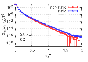
Figure 1: The conserved-conserved (CC) renormalized non-static and static screening correlators in the first Matsubara-sector on our finest ensemble called X7 ($a\sim$ 0.033 fm).

3 Lattice setup

In order to calculate the screening correlators which enter the expression (5) for $H_{E}$, we used three ensembles generated at the same temperature in the high-temperature phase ($T\sim 250$ MeV). We employ two-flavors, O($a$)-improved dynamical Wilson fermions and the plaquette gauge action. The zero-temperature pion mass in our study is around $m_{\pi}\approx 270$ MeV, and the lattice spacings are in the range of 0.033–0.05 fm. We use the isovector vector current instead of the electromagnetic current, whereby disconnected contributions are absent. The Euclidean correlators at imaginary spatial momentum have been measured using the local as well as the conserved discretizations of the currents both at source and sink, resulting in total of four different discretizations (local-local, conserved-conserved, local-conserved and conserved-local). The two mixed discretizations are not independent, they can be transformed into each other using Cartesian coordinate reflections. After averaging these appropriately, we had therefore three different discretizations of the correlators. At each ensemble we had around 1500–2000 configurations and 64 point sources per configuration. We renormalized the local-local and the mixed correlators by multiplying by $Z_{V}^{2}$ or $Z_{V}$, respectively. We took the corresponding value for $Z_{V}$ from Ref. [16].

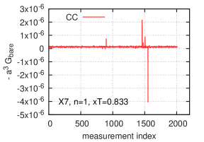
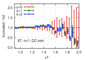
Figure 2: Left panel: Measurement history of the non-static screening correlator at $xT=0.833$. The outliers are shown up as spikes in the data. Right panel: Truncation stability for the non-static screening correlator. The data points corresponding to the trimmed data have been shifted slightly to the right to improve visibility.

We occasionally encountered results for the correlator at a certain Euclidean distance with several standard deviations off from the mean value at that distance, which we identified as outliers, see the left panel of Fig. 2. These occured more frequently at larger Euclidean separations. These outliers increased the statistical error and also modified the mean to some extent, see Fig. 2, right panel. We eliminated these outliers by using robust statistics [17]. First, we prepared a distribution of results at each Euclidean distance, then removed the data points belonging to the lower and upper $\gamma$% of that distribution. We varied $\gamma$ between 0.5–4 when making these cuts and found that the error estimation as well as the calculation of the mean is more stable this way. In the final analysis we used $\gamma=1$, but when we detected only less than 10 datapoints being outside five times the interquantile range from the mean, we only applied trimming with $\gamma=0.5$. We show an example in case of the conserved-conserved correlator at our finest ensemble, X7, in the right panel of Fig. 2. At short distances of the correlator, this approach did not influence the results, because outliers occured there only very rarely. At intermediate distances, i.e. around $xT\sim$0.7–1.3, the effect of this method was again not significant. At large distances, however, the errors reduced by a factor of around 2–6 when omitting the tails of the distributions. Since we believe that these outliers are not likely to have physical origin, their exclusion should not influence the validity of the extracted physical results. This is indeed what we found when analyzing the data without truncating: we obtained consistent final results but with larger errors.

4 Modeling the tail of the screening correlators

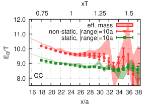
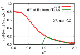
Figure 3: Left: fitted masses and effective masses for the non-static and static screening correlators using a fit range of 10$a$. Right: the integrand needed for the calculation of $H_{E}$ at the first Matsubara-frequency.

Since the integral of Eq. (5) receives contributions from large distances as well, we need to get good control over the screening correlators at large distances, if we aim at a precise determination of $H_{E}$.

The screening correlators have a representation in terms of energies and amplitudes of screening states in the following form [13]:

$$G_{\rm{ns}}(\omega_{r},x_{3})\overset{x_{3}\neq 0}{=}\sum_{n=0}^{\infty}|A_{\rm{ns},n}^{(r)}|^{2}e^{-E_{\rm{ns},n}^{(r)}|x_{3}|}.$$ (6)

A similar expression holds for the static correlator. The low-lying screening spectrum can be studied using weak-coupling methods as well [18]. The lowest energy of a screening state in a given Matsubara sector with frequency $\omega_{r}$ is often called the screening mass and is denoted by $E^{(r)}_{0}$.

In order to get a better handle on the asymptotic behavior of the screening correlators and avoid the enhancement of the error on $H_{E}$ coming from fluctuations present in the actual correlators at large distances, we performed single-state fits on the tails of the correlators using the above representation translated to a form corresponding to a periodic lattice, namely

$$G_{\rm{ansatz}}(\omega_{r},x_{3})=|A_{0}^{(r)}|^{2}\cosh\big{[}E^{(r)}_{0}(x_{3}-L/2)\big{]},$$ (7)

$L$ being the spatial length of the lattice. While the single-state fits describe the actual data well, i.e. with good $\chi^{2}$- and p-values, the identification of the plateau region was not clear in several cases, although we performed a thorough scan using all possible fit ranges having different starting points and different lengths with 6$a$–11$a$. Besides fitting, we also determined the "effective mass" using two consecutive correlator datapoints, by solving

$$\frac{G(\omega_{r},x_{3}+a)}{G(\omega_{r},x_{3})}=\frac{\cosh\big{[}m_{\rm{eff}}(x_{3}+a-L/2)\big{]}}{\cosh\big{[}m_{\rm{eff}}(x_{3}-L/2)\big{]}}$$ (8)

for $m_{\rm{eff}}$. The effective masses are in quite good agreement with the fitted masses, but also do not show a clear plateau as $x_{3}$ increases, see Fig. 3, left panel. Therefore, we decided to choose three representatives from a histogram built by assigning Akaike-weights [19, 20] to all the fitted masses that we obtained. We propagate the median as well as the values near the 16th and 84th percentiles to the later steps of the analysis. When proceeding this way for the non-static as well as for the static screening correlators, we obtain $3\times 3=9$ possibilities for modeling the tail of the integrand of Eq. (5) on a given ensemble. We calculated $H_{E}$ using all these nine combinations for the tail, sorted the results and then chose the median, the values near the 16th and near the 84th percentile after assigning uniform weights for these slightly different values of $H_{E}$. Thus for each ensemble we had three representative values of $H_{E}$ that went into the next step of the analysis, which was the continuum extrapolation. We note that by modeling the tail of the non-static and static screening correlators by doing single-state fits, we could reduce the errors by a factor of around 2.5 on our coarsest ensemble. The transition to the modelled tail has been introduced smoothly by using a step function and we investigated the effect of choosing different switching points, $x_{w}$, in the range $x_{w}T$=0.8–1.2. We found that the results were essentially stable against these choices.

5 Continuum extrapolation

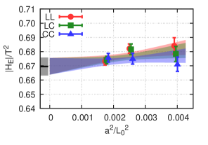
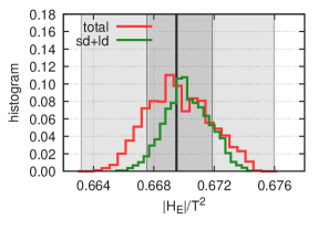
Figure 4: Left: a representative continuum limit of $H_{E}$. Right: histogram of the Akaike-weights plotted against the continuum extrapolated results. The AIC-weighted histogram of the long-distance contribution to $H_{E}$ shifted with the continuum result for the short-distance contribution is also shown for comparison (sd+ld) and are in agreement with the AIC-weighted histogram of the continuum extrapolated results of the total $H_{E}$.

The three discretized correlators allowed us to perform a correlated simultaneous continuum extrapolation of $H_{E}$. We used a linear ansatz in $a^{2}$ when extrapolating to the continuum.

As discussed in the previous section, in order to have a more precise value we modelled the tail of the integrand needed to evaluate $H_{E}$. Since this way at each ensemble and for each discretization we had three representative values of $H_{E}$, we used these in all possible combinations when performing the continuum limit. These gave a total of $(3^{3})^{3}=19683$ different continuum extrapolations of which we built an AIC-weighted histogram to estimate the systematic error. A representative continuum extrapolation as well as the histogram are shown in Fig. 4, left and right panel, respectively.

We also performed separate continuum extrapolations of the short- as well as of the long-distance contributions. In the case of the short-distance contribution, we simply integrated using the trapezoid formula and the systematic error of the continuum extrapolation has been estimated by omitting one of the discretizations at the coarsest ensemble. By shifting the Akaike-weighted histogram of the continuum extrapolated values of the long-distance contribution with the central value of the continuum extrapolated short-distance contribution, we observe that it is consistent with the continuum extrapolated values of the total $H_{E}$ (Fig. 4, right panel).

6 Comparisons

observable	value at the continuum limit
$|H_{E}|/T^{2}$	$0.670(6)_{\rm stat}(2)_{\rm sys}$
sd($x_{\rm w}T=1)$	$0.579(3)_{\rm stat}(1)_{\rm sys}$
ld($x_{\rm w}T=1)$	$0.091(5)_{\rm stat}(2)_{\rm sys}$

Table 1: Results in the first Matsubara sector using single-state fits to model the tail of the integrand.

For the purpose of comparison, it is worth calculating the imaginary part of the retarded correlator at the lightcone in the free theory as well as in strongly coupled $\mathcal{N}=4$ super Yang–Mills theory using the AdS/CFT correspondence. This has been done in Ref. [13]. In the free theory, $|H_{E}|/T^{2}=0.5$ in the first Matsubara sector, while in $\mathcal{N}=4$ super Yang–Mills theory, $|H_{E}|/T^{2}\approx 0.75$. When normalizing with the temperature, the lattice result we obtained, $0.670(6)_{\rm{stat}}(2)_{\rm{sys}}$, is between these two values. Using another normalization might also be interesting. When dividing by the static susceptibility, $\chi_{s}$, of the relevant theories, we obtain in the first Matsubara sector the following results: $[|H_{E}|/\chi_{s}]^{\rm{(free)}}=0.5$ in the free theory (because $\chi_{s}^{\rm{(free)}}/T^{2}=1$), $[|H_{E}|/\chi_{s}]^{\rm{(SYM)}}\approx 0.67$ in $\mathcal{N}=4$ super Yang–Mills theory with $N_{c}=3$. On the lattice, we determined the static susceptibility in Ref. [12] to be $\chi_{s}^{\rm{(lat)}}/T^{2}=0.882(11)_{\rm{stat}}(19)_{\rm{sys}}$. Using this normalization, the lattice result is $[|H_{E}|/\chi_{s}]^{\rm{(lat)}}\approx 0.76$ that is about 13% larger than the value in $\mathcal{N}=4$ SYM theory.

7 Conclusions and outlook

In this contribution, we calculated Euclidean correlators at imaginary spatial momentum, that are related to the thermal photon emission rate according to Eq. (3). We focused on the correlator evaluated at the first non-vanishing Matsubara frequency. In order to improve the predictive power of our result we modelled the tail of the screening correlators occuring in the integrand for our primary quantity $H_{E}$. We were able to describe the data with single-state fits with good p-values. We performed a simultaneaous correlated continuum extrapolation of the three lattice discretizations of the imaginary momentum correlator using three thermal ensembles. The result we obtained is in the same ballpark as obained in the free theory or in $\mathcal{N}=4$ supersymmetric Yang–Mills theory. Depending on the normalization it could be between these two, or larger than these results.

As noted in Ref. [13], the knowledge of $H_{E}(\omega_{n})$ for all $n>n_{0}$ would enable one to determine the spectral function uniquely by Carlson’s theorem. Following a similar route for analyzing $H_{E}$ in the second Matsubara-sector, however, revealed that the signal will soon become noisy and the uncertainty of $H_{E}(\omega_{n=2})$ is therefore much larger. At present our determination of $H_{E}(\omega_{n=2})$ is compatible within errors with the $H_{E}(\omega_{n=1})$ result. We note, however, that since $\sigma(\omega)>0$, $|H_{E}(\omega_{r})|$ has to be larger than $|H_{E}(\omega_{n})|$ if $r>n$  [13, 15]. In order to have a reliable calculation of $H_{E}(\omega_{n\geq 2})$, one has to implement algorithmic improvements and/or devise other operators which could help to constrain the long-distance behavior of the screening correlators. The exploration of these directions is left for future work.

8 Acknowledgements

This work was supported by the European Research Council (ERC) under the European Union’s Horizon 2020 research and innovation program through Grant Agreement No. 771971-SIMDAMA, as well as by the Deutsche Forschungsgemeinschaft (DFG, German Research Foundation) through the Cluster of Excellence “Precision Physics, Fundamental Interactions and Structure of Matter” (PRISMA+ EXC 2118/1) funded by the DFG within the German Excellence strategy (Project ID 39083149). T.H. is supported by UK STFC CG ST/P000630/1. The generation of gauge configurations as well as the computation of correlators was performed on the Clover and Himster2 platforms at Helmholtz-Institut Mainz and on Mogon II at Johannes Gutenberg University Mainz. We have also benefitted from computing resources at Forschungszentrum Jülich allocated under NIC project HMZ21. For generating the configurations and performing measurements, we used the openQCD [21] as well as the QDP++ packages [22], respectively.

References

- [1] Adcox, K. et al., PHENIX coll. Formation of dense partonic matter in relativistic nucleus-nucleus collisions at RHIC: Experimental evaluation by the PHENIX collaboration Nucl. Phys. A, Vol. 757, 184–283, 2005 [arXiv:nucl-ex/0410003]
- [2] Gabor David, Direct real photons in relativistic heavy ion collisions Rept. Prog. Phys. 83, 4, 046301 (2020) [arXiv:nucl-ex/1907.08893]
- [3] Gale, Charles and Paquet, Jean-François and Schenke, Björn and Shen, Chun, Multi-messenger heavy-ion physics [arXiv:nucl-th/2106.11216]
- [4] Jackson, G., Two-loop thermal spectral functions with general kinematics Phys. Rev. D 100, 11, 116019 (2019) [arXiv:hep-ph/1910.07552]
- [5] Jackson, G. and Laine, M., Testing thermal photon and dilepton rates JHEP 11, 144 (2019) [arXiv:hep-ph/1910.09567]
- [6] Caron-Huot, Simon and Kovtun, Pavel and Moore, Guy D. and Starinets, Andrei and Yaffe, Laurence G., Photon and dilepton production in supersymmetric Yang-Mills plasma JHEP 12 (2006) 015 [arXiv:hep-th/0607237]
- [7] Meyer, Harvey B., Transport Properties of the Quark-Gluon Plasma: A Lattice QCD Perspective Eur. Phys. J. A, Vol. 47, p86, 2011 [arXiv:hep-lat/1104.3708]
- [8] Aarts, Gert and Nikolaev, Aleksandr, Electrical conductivity of the quark-gluon plasma: perspective from lattice QCD Eur. Phys. J. A, Vol. 57, No. 4, p118, 2021 [arXiv:hep-lat/2008.12326]
- [9] Kaczmarek, Olaf and Shu, Hai-Tao, Spectral and Transport Properties from Lattice QCD Lect. Notes Phys., Vol. 999, p307–345, 2022 [arXiv:hep-lat/2206.14676]
- [10] Ghiglieri, J. and Kaczmarek, O. and Laine, M. and Meyer, F., Lattice constraints on the thermal photon rate Phys. Rev. D, Vol. 94, No. 1, 016005, 2016 [arXiv:hep-lat/1604.07544]
- [11] Cè, Marco and Harris, Tim and Meyer, Harvey B. and Steinberg, Aman and Toniato, Arianna, Rate of photon production in the quark-gluon plasma from lattice QCD Phys. Rev. D, Vol. 102, No. 9, 091501, 2020 [arXiv:hep-lat/2001.03368]
- [12] Cè, Marco and Harris, Tim and Krasniqi, Ardit and Meyer, Harvey B. and Török, Csaba Photon emissivity of the quark-gluon plasma: A lattice QCD analysis of the transverse channel Phys. Rev. D, Vol. 106, No. 5, p. 054501, 2022 [arXiv:hep-lat/2205.02821]
- [13] Meyer, Harvey B., Euclidean correlators at imaginary spatial momentum and their relation to the thermal photon emission rate Eur. Phys. J. A, Vol. 54, No. 11, p192, 2018 [arXiv:hep-lat/1807.00781]
- [14] McLerran, Larry D. and Toimela, T. Photon and Dilepton Emission from the Quark - Gluon Plasma: Some General Considerations Phys. Rev. D, Vol. 31, p545, 1985
- [15] Meyer, Harvey B. and Cè, Marco and Harris, Tim and Toniato, Arianna and Török, Csaba Deep inelastic scattering off quark-gluon plasma and its photon emissivity PoS, LATTICE2021, p269, 2022 [arXiv:hep-lat/2112.00450]
- [16] Dalla Brida, Mattia and Korzec, Tomasz and Sint, Stefan and Vilaseca, Pol High precision renormalization of the flavour non-singlet Noether currents in lattice QCD with Wilson quarks Eur. Phys. J. C, Vol. 79, No. 1, p23, 2019 [arXiv:hep-lat/1808.09236]
- [17] Peter J. Huber, Elvezio M. Ronchetti Robust Statistics, 2nd edition John Wiley and Sons, 2009
- [18] Brandt, B. B. and Francis, A. and Laine, M. and Meyer, H. B. A relation between screening masses and real-time rates JHEP, Vol. 05, p117, 2014 [arXiv:hep-ph:1404.2404]
- [19] H. Akaike Information theory and an extension of the maximum likelihood principle Proceedings for 2nd International Symposium on Information Theory, Tsahkadsor, Armenia, USSR, September 2-8, Budapest: Akadémiai Kiadó, pp.267-281, 1971
- [20] Borsanyi Sz. and others, Leading hadronic contribution to the muon magnetic moment from lattice QCD Nature, Vol. 593, No. 7857, p. 51–55, 2021 [arXiv:hep-lat/2002.12347]
- [21] Lüscher, Martin and Schäfer, Stefan Lattice QCD with open boundary conditions and twisted-mass reweighting Comput. Phys. Commun., Vol. 184, 519-528, 2013 [arXiv:hep-lat/1206.2809]
- [22] Edwards, Robert G. et al. The Chroma software system for lattice QCD Nucl. Phys. B Proc. Suppl., Vol. 140, p. 832, 2005 [arXiv:hep-lat/0409003]