Decomposition of the Leinster-Cobbold Diversity Index
Abstract.
The Leinster and Cobbold diversity index (Leinster and Cobbold, 2012) possesses a number of merits; in particular, it generalises many existing indices and defines an effective number. We present a scheme to quantify the contribution of richness, evenness, and taxonomic similarity to this index. Compared to the work of (van Dam, 2019), our approach gives unbiased estimates of both evenness and similarity in a non-homogeneous community. We also introduce a notion of taxonomic tree equilibration which should be of use in the description of community structure.
Keywords: diversity, similarity, evenness, richness, decomposition, Leinster–Cobbold diversity index.
1. Introduction
Measuring biodiversity is a difficult task due to sampling issues and accounting for missing data, but also as there is no one universally accepted definition of what biodiversity is (Daly et al., 2018). In ecological practice, definitions of biodiversity can include contributions from multiple channels of information such as the number of species (“richness”), dominance or rarity relations among the constituent species (“evenness”), and measures of “similarity” among the species (estimated either from taxonomic or phylogenetic relationships, or from functional traits relationships) (Purvis and Hector, 2000; Leinster and Cobbold, 2012). Biogeographic patterns of diversity can depend on the definitions used. For example, (Stuart-Smith et al., 2013) showed that biodiversity hotspots can shift from the tropics to higher latitudes if one only considers abundances or also takes account of functional traits similarity of species.
An outstanding challenge in the field of conservation ecology is to relate the various aspects of biodiversity data to the functioning of ecosystems (Maureaud et al., 2019; Hillebrand et al., 2018).
Thus the goal is to construct a biodiversity index that would carry information about as many aspects of diversity as possible. This goal has been actively pursued (Rao, 1982; Leinster and Cobbold, 2012; Chao et al., 2014). By “carrying information” we means that, for example, we should be able to extract information about richness or evenness from our index. One way of extracting such information is to decompose the index additively or multiplicatively into components that can be interpreted in a biologically meaningful way; see for example discussions of - - and - diversity (Jost, 2007; Anderson et al., 2011). A priori it is not clear why such a decomposition would exist, whether it has to be unique, and in cases of non-uniqueness, what are the conditions for optimality of a decomposition.
As an example of this approach, van Dam (van Dam, 2019) has recently proposed a straightforward decomposition of the Leinster–Cobbold (LC) index (Leinster and Cobbold, 2012). In a sense, our work below is a generalisation of the work of van Dam, which uses intrinsic properties of the LC index to remove an important bias in van Dam’s decomposition with intriguing and far-reaching consequences.
The structure of the paper is as follows. In Section 2 we discuss the definitions of richness, evenness and similarity using (Chao et al., 2014; Chiu et al., 2014; Daly et al., 2018; Gregorius and Gillet, 2022). In Section 3 we collect the required information about the LC index following (Leinster and Cobbold, 2012; Leinster and Meckes, 2016); it subsumes many other diversity indices such Rao’s index that is widely used in functional ecology (Rao, 1982; Ricotta and Moretti, 2011). In Section 4 we present van Dam’s and then our decomposition and its consequences. Finally, in Section 6 we discuss the relation of our work to that or Chao and Ricotta (Chao and Ricotta, 2019), extensions and open problems.
2. Diversity components
2.1. Notation
First of all, we need to establish notation. Everywhere below we assume that the number of species in a community is fixed at .
We will use to denote the vector of relative abundances, and let
| (1) |
be the standard -simplex in .
Remark 1.
It has to be emphasised that admissible relative abundance vectors take values in , the interior of :
| (2) |
which is not a closed set in ; the consequence of that is that there are converging sequences in , whose limit is contained in the boundary ; such limits by necessity correspond to communities with fewer than species.
We will often use the vector
| (3) |
the subscript stands for “homogeneous”. is the relative abundance of a community where each species is represented equally. We denote by the set of -vectors having one component equal to 1 and the rest equal to zero. Thus, is the relative abundance vector of a monomorphic community. will stand below for an -vector with all components equal to .
Next, we need to discuss sets of matrices. First of all, we will denote the identity matrix by . We will use the notation for the matrix of ones.
In the present paper, for simplicity, we will be working with ultrametric matrices; this choice is motivated by the fact that similarity matrices (see subsection 3.1) constructed using taxonomic trees are necessarily ultrametric and since using them simplifies the theory of (Leinster and Meckes, 2016). For more information on ultrametric matrices, please see (Dellacheria et al., 2014, Ch. 3) and (Leinster, 2013; Leinster and Meckes, 2016). We will denote that set of all ultrametric matrices by and its interior by .
Definition 2 (Defn. 3.2 of (Dellacheria et al., 2014)).
A symmetric matrix is ultrametric if , and , .
Remark 3.
Note that in (Leinster and Meckes, 2016, Example 12) Leinster and Meckes take the matrices they call ultrametric to be strictly diagonally dominant. That would preclude the set of ultrametric matrices from being closed; so in our definition .
2.2. Evenness
The concept of evenness (for which see, e.g. (Chao et al., 2014; Chao and Ricotta, 2019; Gregorius and Gillet, 2022)) and references therein), is rather problematic. First of all, the terminology is badly chosen as it would immediately seem that the “most even” population of species is one for which the vector of relative abundances is the homogeneous vector , i.e. one where every species is equally represented. Thus, like the case of richness discussed below, the terminology seems to be precluding discussion. As rightly pointed in (Gregorius and Gillet, 2022), such a categorical answer to the question of maximal evenness leaves open the discussion of what would constitute “maximum unevenness” in . van Dam (van Dam, 2019) uses instead the concept of “balance”, which seems to us a better term; this is the concept which, after defining it properly (see (11)) we will be using below.
2.3. Richness
Richness is sometimes summarily defined to be the number of species, see e.g. (Daly et al., 2018). Our approach below allows us to retain this definition but at a price. Such a definition is open to the same criticism as the notion of maximal evenness defined by that we have discussed above. It is again “species-centric”, and takes into account only the last level of taxonomic classification. Below, in Section 4 we suggest how to introduce a defensible new notion of richness that uses taxonomic information.
2.4. Similarity
In this section we discuss the construction of taxonomic similarity matrices for a community with species.
The usual way of constructing similarity matrices which are automatically ultrametric is to assign distances between different levels of a taxonomic tree. Then the taxonomic distance between two species is the sum of distance from the nodes corresponding to these species to the first common node, and then one puts or if the maximal distance in the tree has been normalised to 1, one could put . As a example, consider the tree in Figure 1
and set the species-genus and the genus-family distance to be . If we use the additive recipe, we get
| (4) |
3. The Leinster–Cobbold diversity index
In their influential paper (Leinster and Cobbold, 2012), Leinster and Cobbold introduced a far-reaching generalisation of Hill numbers, for discussions of which see (Chiu et al., 2014; Hill, 1973), the LC index. For details on its properties, see (Leinster and Cobbold, 2012; Leinster and Meckes, 2016); here we just collect the bare minimum in the framework of taxonomic (ultrametric) similarity matrices.
3.1. Definition of the LC index
As in the definition of Hill numbers, below is the sensitivity parameter, measuring the importance given to rare species. Then for a community of species with relative abundance vector and (ultrametric) similarity matrix , we have
Definition 4.
The LC diversity of order is
| (5) |
Note that (Leinster and Cobbold, 2012) use a different notation, similar to the Hill number notation in the literature; they denote the right-hand side of (5) by . We prefer the notation used here as it clearly shows functional dependencies and allows easy generalisation, which we discuss briefly in Section 6. We collect the required properties of the LC index in the proposition below and in subsection 3.2.
Proposition 5.
Let . . Then
-
[(a)]
-
(1)
is a monotone decreasing function of ;
-
(2)
for all if ;
-
(3)
for all ;
-
(4)
for all .
For proofs of (a) and (b) please see (Leinster and Cobbold, 2012); the rest are immediate.
Following (Leinster and Meckes, 2016), we now discuss the concept of a maximally balanced abundance vector for a community of species with an ultrametric similarity matrix .
3.2. A crucial property of the LC index
Using only ultrametric taxonomic similarity matrices simplifies the presentation considerably. For the more general case where the similarity matrix is simply a symmetric matrix with positive elements, see (Leinster and Meckes, 2016). The results of that paper have not, in our opinion, been sufficiently seriously considered by the biodiversity community.
We present two theorems from (Leinster and Meckes, 2016). First of all we have the following existence and uniqueness result for maximisers of the LC diversity index.
Theorem 6.
For each there exists a unique abundance vector that maximises for every value of .
Definition 7.
Given , we call the corresponding abundance vector the maximally balanced abundance vector.
This is the vector that corresponds to that arises in theories that do not take into account taxonomic similarity.
Computing the maximally balanced vector in the case of ultrametric similarity matrices is a simple matter of solving a system of linear equations and normalising. If the similarity matrix is not ultrametric, the situation is more complex; see (Leinster and Meckes, 2016) for details.
Theorem 8.
Given , is given by
where solves the system of equations , where is a column vector of ones.
Note that (Leinster and Meckes, 2016, Lemma 6) provides an alternative way of computing .
Definition 9.
A taxonomic tree will be called taxonomically equilibrated if .
Of course we have
Proposition 10.
If at each level of the tree all the nodes have the same degree, the taxonomic tree is equilibrated.
The converse of Proposition 10 does not hold, i. e. there are taxonomic graphs that do not satisfy the conditions of that proposition, for which a metric can be assigned such that the resulting is . An example is provided by the following tree:
It is not hard to show that the assignment of species-genus, genus-family and family-order distances of and using the additive recipe, results in a similarity matrix for which . Thus there is a trichotomy of taxonomic trees: those in Proposition 10 is which holds for every assignment of distances; those where such assignments can be chosen, as in Figure 2, and such that no assignment of distances results in a homogeneous maximally balanced abundance vector; an example of such a tree is in Figure 3.
We will discuss this trichotomy in more detail in (Chen and Grinfeld, 2023).
Remark 11.
Compared to the diversity metrics proposed by Chao et al. (Chao et al., 2014), the LC index has the flexibility to take into account taxonomic, phylogenetic, and functional diversity simultaneously. However in that case the resulting similarity matrices are no longer ultrametric and we leave that more general case for future study. Also note that the above trichotomy of taxonomic trees would not necessarily exit if there were a canonical way of constructing similarity matrices.
4. An unbiased decomposition scheme
We are now ready to propose a decomposition scheme for the LC index. It is best to start with the decomposition scheme proposed by van Dam (van Dam, 2019) and see why it has to be modified. van Dam writes
| (6) |
The first fraction is clearly a measure of dissimilarity, while the second fraction is a measure of balance; of course , so the last term in the right-hand side is a richness. From many points of view, this is a good decomposition as the two fractions always lie in the interval . Consult Proposition 5 to see that the infimum is never reached. The problem here is with the definition of the measure of balance, as it does not take into account the taxonomic similarity matrix while the dissimilarity measure uses information from both and . We call such a decomposition asymmetrically biased. A different asymmetrically biased decomposition is given by
| (7) |
In this decomposition the first fraction is a measure of balance, the second a measure of dissimilarity, while as before, the last term is richness. Of course here it is the measure of dissimilarity that is asymmetrically biased. A possibility that might be considered of multiplying (6) and (7) and taking the square root. That will give us a decomposition which we would call unbiased (though it could be also called “symmetrically biased”) . However, there is an additional problem in (7) which is that the first fraction in the right-hand side can take values larger than one if for example, is not a similarity matrix of a taxonomically equilibrated tree and . We do not pursue this direction as we do not see any reason for a relative measure not to take values in .
The price of ensuring normalisation is having to deal with richness in more detail. Consider instead of (7), the following decomposition:
| (8) |
It is asymmetrically biased as second factor does not involve . We will discuss the interpretation of later.
To obtain an unbiased decomposition, we therefore multiply (6) and (8) and take a square root. The result is
| (9) |
The last term in the right-hand side can be rewritten as
| (10) |
The term expresses the lack of equilibration in the taxonomic tree; see Definition 9 and Theorem 10.
Putting
| (11) |
| (12) |
We finally write our decomposition as
| (13) |
i.e. a product of measures of balance , dissimilarity , (lack of) equilibration and the classical richness .
Note that by construction both the measure of balance (11) and dissimilarity (12) are constrained to lie in by Proposition 5.
Both the measure of balance and of dissimilarity are geometric means of an unbiased measure and a biased one. It does not seem possible to find a truly unbiased decomposition of the LC index, which is the reason we could call the decomposition (13) symmetrically biased.
Note that though (the right-hand side being independent of ), it is not clear what vector maximises it for a particular value of . Of course the value is reached for by the choice .
depends on , as defines , and hence reflects the structure of the underlying taxonomic tree. Note that in the case of similarity matrices of taxonomically equilibrated trees, for which we have and hence , so that , If does not correspond to a taxonomically equilibrated taxonomic tree, is dependent on .
5. Practical examples
To illustrate how our decomposition approach differs from the “ABC” approach suggested by van Dam (van Dam, 2019), we use a simple example in Leinster and Cobbold (Leinster and Cobbold, 2012) (their Example 3; original data from (DeVries et al., 1997)). This example has the nice feature that the difference between the two communities changes the sign when increases from 0 to 2.
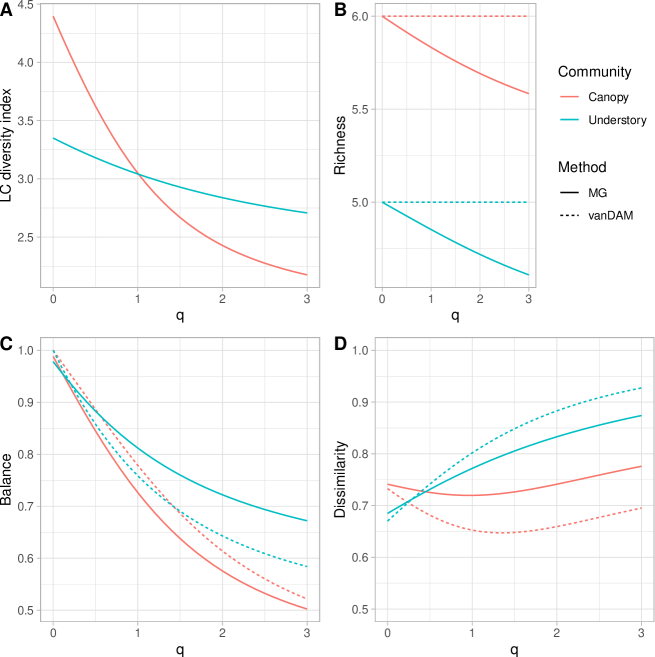
Compared to van Dam (van Dam, 2019), our new decomposition approach yields different interpretations regarding what aspects of diversity lead to the differences in diversity estimates between the two communities (Canopy vs. Understory). When we put more emphasis on rare species (), the Canopy community is more diverse because it has a larger number of species richness (6 vs. 5) and its species are slightly more dissimilar with each other (Fig. 4A,D). By contrast, when we focus more on abundant species (), the Understory community becomes more diverse because of its greater balance (evenness) of dominant species (Fig. 4A,C). The difference between our decomposition approach and van Dam (van Dam, 2019) is that our approach predicts a much larger difference in Balance than van Dam (van Dam, 2019) (and a smaller difference in species dissimilarity) when we increasingly focus on dominant species (larger ). Our approach also shows that as increases, the Understory community shows a stronger lack of equilibration (i.e., deviation of from ) than the Canopy community, albeit this difference is small. In summary, we would interpret that the greater diversity of the Understory community when we focus on dominant species is because its dominant species are more balanced than those in the Canopy community. On the contrary, the interpretation would be that the dominant species are more dissimilar to each other in the Understory community if we use the approach of van Dam (van Dam, 2019).
6. Discussion
The LC index uses three “information streams”: the number of species (richness) , the relative abundance vector and the similarity matrix . We could in theory consider a diversity index , where are information streams, sources of information about the structure of the community, expressed as some mathematical objects (vectors, matrices higher order tensors). We could then follow the decomposition process of Section 4: find biased decompositions, multiply them together and take the -root. However, this is already unwieldy in the case of . But note that this procedure is unnecessary as the LC theory has a lot of built-in flexibility in the definition of similarity matrices. As explained in subsection 2.4, one can define a similarity matrix by setting , where is some suitably defined distance between species and . Hence incorporating more information streams can be thought about as changing the distance function ; in the process of incorporating such information, such as functional similarity, the ultrametricty of the similarity matrix is lost; it is possible that the resulting function will no longer be a metric, becoming more generally a divergence measure. The point is and (a suitably redefined) dependence of a diversity index is sufficient to incorporate all relevant information.
In (Chao and Ricotta, 2019), Chao and Ricotta show how to quantify evenness using divergence measures. It is useful therefore to consider the LC diversity index (4) in this context. As now we deal with balance as opposed to evenness, we will denote the resulting balance index by . First of all, let us note that (11) cannot give rise to an divergence measure-based index of balance as there is no well defined upper bound for it for all . It is still of course useful in providing an estimate of the balance contribution to the LC diversity index. These two statements are not in contradiction.
Clearly, the LC index itself provides a divergence measure-based estimate (index) of balance via
| (14) |
where one could alternatively write where is any vector in .
Concerning similarity indices, it again does not seem to be possible to utilise of (12) to this end. On the other had, the LC index itself provides a divergence measure based similarity index by
| (15) |
Again, here the value 1 is never reached over . It is not hard to show the following proposition:
Proposition 13.
The indices , satisfy all the requirements in (Chao and Ricotta, 2019).
To conclude, we have proposed a novel decomposition of the LC index. Compared to a previous version of decomposition due to van Dam (van Dam, 2019), our approach estimates the balance and dissimilarity of the community more comprehensively (e.g., we not only estimate dissimilarity for a homogeneous community but also consider the present vector of relative abundance). As such, we believe that our inference is more robust when comparing balance and dissimilarity among communities. In addition, we had by necessity to introduce a notion of taxonomic tree equilibration (which turns out to be an important concept in our on-going work on quantifying un-evenness (Chen and Grinfeld, 2023)), which is another descriptor of a biological community. We advocate the use of our decomposition (13) as a “maximally unbiased” estimate of contributions of balance and (dis)similarity to diversity.
References
- Anderson et al. (2011) Anderson, M. J., Crist, T. O., Chase, J. M., Vellend, M., Inouye, B. D., Freestone, A. L., Sanders, N., Cornell, H., Comita, L., Davies, K., and Harrison, S. (2011). Navigating the multiple meanings of diversity: a roadmap for the practicing ecologist. Ecology Letters, 14:19–28.
- Chao et al. (2014) Chao, A., Chiu, C.-H., and Jost, L. (2014). Unifying species diversity, phylogenetic diversity, functional diversity, and related similarity differentiation measures through Hill numbers. Annual Review of Ecology, Evolution, and Systematics, 45:297–324.
- Chao and Ricotta (2019) Chao, A. and Ricotta, C. (2019). Quantifying evenness and linking it to diversity, beta diversity and similarity. Ecology, 100:e02852.
- Chen and Grinfeld (2023) Chen, B. and Grinfeld, M. (2023). An evennesss index based on the Leinster–Cobbold diversity index. in progress.
- Chiu et al. (2014) Chiu, C.-H., Jost, L., and Chao, A. (2014). Phylogenetic beta diversity, similarity, and differentiation measures based on Hill numbers. Ecological Monographs, 81:21–44.
- Daly et al. (2018) Daly, A. J., Baetens, J. M., and De Baets, B. (2018). Ecological diversity: measuring the unmeasurable. Mathematics, 6:119.
- Dellacheria et al. (2014) Dellacheria, C., Martinez, S., and San Martin, J. (2014). Inverse M-matrices and Ultrametric Matrices. Springer.
- DeVries et al. (1997) DeVries, P. J., Murray, D., and Lande, R. (1997). Species diversity in vertical, horizontal, and temporal dimensions of a fruit-feeding butterfly community in an ecuadorian rainforest. Biological Journal of the Linnean Society, 62(3):343–364.
- Gregorius and Gillet (2022) Gregorius, H.-R. and Gillet, E. M. (2022). The concept of evenness/unevenness: less evenness or more unevenness? Acta Biotheoretica, 70:1–28.
- Hill (1973) Hill, M. (1973). Diversity and evenness: a unifying notation and its consequences. Ecology, 54:427–432.
- Hillebrand et al. (2018) Hillebrand, H., Blasius, B., Borer, E. T., Chase, J. M., Downing, J. A., Eriksson, B. K., Filstrup, C. T., Harpole, W., Hodapp, D., Larsen, S., and Lewandowska, A. M. (2018). Biodiversity change is uncoupled from species richness trends: Consequences for conservation and monitoring. Journal of Applied Ecology, 55(1):169–184.
- Jost (2007) Jost, L. (2007). Partitioning diversity into independent alpha and beta components. Ecology, 88:2427–2439.
- Leinster (2013) Leinster, T. (2013). The magnitude of metric spaces. Documenta Mathematica, 18:857–905.
- Leinster and Cobbold (2012) Leinster, T. and Cobbold, C. (2012). Measuring diversity: the importance of species similarity. Ecology, 93:477–489.
- Leinster and Meckes (2016) Leinster, T. and Meckes, M. W. (2016). Maximizing diversity in biology and beyond. Entropy, 18:88.
- Maureaud et al. (2019) Maureaud, A., Hodapp, D., van Denderen, P. D., Hillebrand, H., Gislason, H., Spaanheden Dencker, T., Beukhof, E., and Lindegren, M. (2019). Biodiversity–ecosystem functioning relationships in fish communities: biomass is related to evenness and the environment, not to species richness. Proceedings of the Royal Society B, 286(1906):20191189.
- Purvis and Hector (2000) Purvis, A. and Hector, A. (2000). Getting the measure of biodiversity. Nature, 405(6783):212–219.
- Rao (1982) Rao, C. R. (1982). Diversity and dissimilarity coefficients: a unified approach. Theoretical population biology, 21(1):24–43.
- Ricotta and Moretti (2011) Ricotta, C. and Moretti, M. (2011). CWM and Rao’s quadratic diversity: a unified framework for functional ecology. Oecologia, 167(1):181–188.
- Stuart-Smith et al. (2013) Stuart-Smith, R. D., Bates, A. E., Lefcheck, J. S., Duffy, J. E., Baker, S. C., Thomson, R. J., Stuart-Smith, J. F., Hill, N. A., Kininmonth, S. J., Airoldi, L., and Becerro, M. A. (2013). Integrating abundance and functional traits reveals new global hotspots of fish diversity. Nature, 501(7468):539–542.
- van Dam (2019) van Dam, A. (2019). Diversity and its decomposition into variety, balance and disparity. Royal Society open science, 6:90452.