FactorJoin: A New Cardinality Estimation Framework for Join Queries

Abstract.

Cardinality estimation is one of the most fundamental and challenging problems in query optimization. Neither classical nor learning-based methods yield satisfactory performance when estimating the cardinality of the join queries. They either rely on simplified assumptions leading to ineffective cardinality estimates or build large models to understand the data distributions, leading to long planning times and a lack of generalizability across queries.

In this paper, we propose a new framework FactorJoin for estimating join queries. FactorJoin combines the idea behind the classical join-histogram method to efficiently handle joins with the learning-based methods to accurately capture attribute correlation. Specifically, FactorJoin scans every table in a DB and builds single-table conditional distributions during an offline preparation phase. When a join query comes, FactorJoin translates it into a factor graph model over the learned distributions to effectively and efficiently estimate its cardinality. Unlike existing learning-based methods, FactorJoin does not need to de-normalize joins upfront or require executed query workloads to train the model. Since it only relies on single-table statistics, FactorJoin has small space overhead and is extremely easy to train and maintain. In our evaluation, FactorJoin can produce more effective estimates than the previous state-of-the-art learning-based methods, with 40x less estimation latency, 100x smaller model size, and 100x faster training speed at comparable or better accuracy. In addition, FactorJoin can estimate 10,000 sub-plan queries within one second to optimize the query plan, which is very close to the traditional cardinality estimators in commercial DBMS.

1. Introduction

Cardinality estimation (CardEst) is a critical component of modern database query optimizers. The goal of CardEst is to estimate the result size of each query operator (i.e., filters and joins), allowing the optimizer to select the most efficient join ordering and physical operator implementations. An ideal CardEst method satisfies several properties: it is effective at generating high-quality query plans, efficient so that it minimizes estimation latency, and easy to deploy in that it has a small model size, fast training times, and the ability to scale with the number of tables and generalize to new queries. Unfortunately, existing CardEst techniques do not satisfy at least one of these properties. The reason behind these failures can largely be reduced to the handling of two related problems: (1) how to characterize attribute correlations and (2) how to model the distribution of join-keys, which directly determine the size of joins.

Background: Many deployed CardEst approaches are still based on the Selinger model (Selinger et al., 1979) and assume attribute independence, where the model ignores correlations between attributes, and join-key uniformity, where the model further assumes that join keys have uniformly distributed values. These assumptions provide a simple way of estimating the cardinality of join queries using only single-table statistics (e.g., histograms) over single attributes, which are easy to create and maintain. As a result, the Selinger-based CardEst techniques are extremely efficient and easy to deploy but at the cost of effectiveness because most real-world datasets contain complex attribute correlations and skewed join-key distributions.

To overcome the limitations of these assumptions, many commercial database systems try to relax them to increase their effectiveness. For example, past works  (Ioannidis, 2003; Ioannidis and Christodoulakis, 1993; Dell’Era, 2007) propose and some systems (e.g. Oracle (Dell’Era, 2017)) employ join-histograms that relax the join-key uniformity assumption. Specifically, these methods build frequency histograms on the join keys and then construct the join distribution by “multiplying” the histograms to estimate the join size (see Figure 1(b)). In this way, these methods can more precisely capture the join-key distributions to generate more effective estimates of the join cardinality. However, they still assume that the join keys are uniformly distributed within each bin of the histogram.

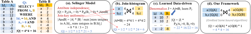
Figure 1. Existing CardEst approaches for handling join queries. (a) The Selinger model writes the cardinality of a two-table join query as the product of filter selectivity $P_{A},P_{B}$ on both tables and the estimated join size $|A\Join B|$. Using join-key uniformity, this is estimated as the product of table sizes $|A|*|B|$ divided by the maximal number of unique values of the join keys. (b) The join-histogram bin the domain of join keys $Id_{1},Id_{2}$ as histograms, assumes join-key uniformity within each bin. (c) The learned data-driven methods de-normalize $J=A\Join B$ and learn the distribution $P_{J}$ to estimate the cardinality of $Q$. (d) Our framework captures the correlation between join keys and filter predicates to accurately estimate $|Q|$ without de-normalization.

Similarly, there have been works on relaxing the attribute independence assumption. For example, multi-dimensional histograms (Deshpande et al., 2001; Gunopulos et al., 2000, 2005; Muralikrishna and DeWitt, 1988; Wang and Sevcik, 2003; Liu et al., 2021b), self-tuning histograms (Bruno et al., 2001; Srivastava et al., 2006; Khachatryan et al., 2015; Fuchs et al., 2007), and singular value decomposition (Poosala and Ioannidis, 1997), have been proposed to capture the correlation between attributes. However, their effectiveness and/or efficiency are still not satisfactory (Yang et al., 2019; Han et al., 2021). More recently, learning-based methods which learn the underlying data distributions (Kipf et al., 2019; Hilprecht, 2019; Zhu et al., 2021; Yang et al., 2019) have been proposed to more accurately and compactly represent the attribute correlations within a single table, but these still have efficiency concerns that we detail below.

Specifically, the learned data-driven methods (Getoor et al., 2001; Tzoumas et al., 2011; Yang et al., 2021; Wu et al., 2020a; Zhu et al., 2021; Hilprecht et al., 2019) analyze data and build distributions for all join patterns in a database. They need to de-normalize the joined tables and add a potentially exponential number of extra columns. Then, they build distributions over the de-normalized tables to characterize all attribute correlations and handle joins (see also Figure 1(c). This allows the learned data-driven methods to be highly accurate for join estimates at the cost of slow training time and large model size (i.e., worse deployability). Alternatively, learned query-driven methods (Kipf et al., 2019; Sun and Li, 2019; Liu et al., 2021a) circumvent the join-key uniformity assumption by building supervised models to map the join queries to their cardinalities. However, they require an impractical number of executed queries to train their models, which is unavailable to new DB instances and do not generalize well to unseen queries.

Our Approach: Surprisingly, we are not aware of any work which tries to combine the advances of learning-based methods for accurately characterizing correlations with the idea of join-histograms. In this work, we develop a novel CardEst framework called FactorJoin that combines these two approaches, i.e., using join-histograms to efficiently handle joins coupled with learning-based methods to accurately capture attribute correlation. This is not a straightforward extension. As we will show, adapting the idea of join-histograms while preserving the benefits of using learning-based methods for attribute correlations is non-trivial. FactorJoin only builds sophisticated models to capture the correlations within a single table. The choice of the model to capture correlation is orthogonal to the techniques of FactorJoin, however, we do require the model to be able to provide conditional distributions of one or more keys. In our current implementation of FactorJoin, we use sampling (Lipton et al., 1990) and Bayesian Networks (Koller and Friedman, 2009) as they are fast to train and execute.

These single-table conditional distributions are then combined using a factor graph model (Loeliger, 2004). Specifically, FactorJoin translates a join query $Q$ into a factor graph over single-table data distributions. This allows us to formulate the problem of estimating the cardinality of $Q$ as a well-studied inference problem (Koller and Friedman, 2009; Loeliger, 2004; Lauritzen, 1996) on this factor graph. Conceptually, there exist some similarities to the join-histogram technique. However, our formulation allows FactorJoin to generalize to cyclic and self-joins. It also improves the computation efficiency by relying on existing inference algorithms (MacKay et al., 2003; Kschischang et al., 2001), and facilitates scaling to arbitrary join sizes. Finally, in contrast to the idea of join-histogram and many other techniques in the space, we propose to actually not estimate the expected join cardinality, but rather use a probabilistic upper bound. As shown by others (Cai et al., 2019; Atserias et al., 2008; Abo Khamis et al., 2017; Hertzschuch et al., 2021), under-estimation is often worse than over-estimation, and tailoring the estimate to a probabilistic upper bound can significantly improve the end-to-end query performance.

As a result, FactorJoin is able to estimate the cardinality of join queries using only single table statistics with similar or better estimation effectiveness than the state-of-the-art (SOTA) learning-based techniques. When compared with the learned data-driven methods, FactorJoin has a much smaller model size, faster training/updating speed, and easier for system deployment because we do not need to denormalize the join tables or add exponentially many extra columns. In addition, FactorJoin supports all forms of equi-joins, including cyclic joins and self joins, as well as complex base table filter predicates, including disjunctive filter clauses and string pattern matching predicates because it can flexibly plug-in various types of base-table estimators to support them. These queries are not supported by the existing learned data-driven methods (Yang et al., 2021; Hilprecht et al., 2019; Zhu et al., 2021), which require the join template to be a tree. Unlikely the learned query-driven methods (Kipf et al., 2019; Sun and Li, 2019; Liu et al., 2021a), FactorJoin does not depend on the executed query workload, so it is robust against data updates and workload shifts, can be quickly adapted to a new DB instance, and is generalizable to new queries. However, in presence of query workload, FactorJoin can incorporate this information to further optimize the model construction process.

We integrate FactorJoin into Postgres’ query optimizer and evaluate its end-to-end query performance on two well-established and challenging real-world CardEst benchmarks: STATS-CEB (Han et al., 2021) and IMDB-JOB (Leis et al., 2015). On the STATS-CEB, FactorJoin achieves near-optimal performance in end-to-end query time. It has comparable performance to the previous SOTA learned data-driven model (FLAT (Zhu et al., 2021)) in terms of estimation effectiveness but with 40x lower estimation latency, 100x smaller model sizes, and 100x faster training times. On the IMDB-JOB, our framework achieves the SOTA performance in end-to-end query time (query execution plus planning time). Specifically, the pure execution time of our framework is comparable to the previous SOTA method (pessimistic estimator (Cai et al., 2019)), but our estimation latency is 100x lower, making our overall end-to-end query time significantly faster. Specifically, our framework can estimate 10,000 sub-plan queries in one second to optimize the query plan, which is close to the planning time of the traditional CardEst method used in Postgres. We also carry out a series of controlled ablation studies to demonstrate the robustness and advantages of different technical novelties of FactorJoin.

In summary, our main contributions are:

$\bullet$ We formulate the problem of estimating the cardinality of join queries in its general form as a factor graph inference problem involving only single-table data distributions (Section 3).

$\bullet$ We propose a new binning and upper bound-based algorithm to approximate the factor graph inference (Section 4).

$\bullet$ We design attribute causal relation exploration and progressive estimation of sub-plan queries techniques to improve the efficiency of our framework (Section 5).

$\bullet$ We conduct extensive experiments to show the advantages of our framework (Section 6).

Before describing the details of FactorJoin, we begin with a detailed description of existing CardEst approaches.

2. Background and analysis

Table 1. Summary of existing CardEst methods.

In this section, we first define the CardEst problem and then analyze existing CardEst methods and how our approach differs from them.

2.1. CardEst problem definition

Single table CardEst: Let $A$ be a table with $n$ attributes $A_{1},\ldots,A_{n}$. A single table selection query $Q(A)$ on $A$ can be viewed a conjunction or disjunction of filter predicates over each attribute, e.g. $Q(A)=(A_{1}\in[0,5])\ \lor$ $(A_{2}$ LIKE ‘%An%’$)\land(A_{5}\leq-10)$.

Let $|Q(A)|$ denote the cardinality of $Q(A)$, i.e. the number of tuples in $A$ satisfying $Q(A)$. Let $P_{A}(Q(A))$ denotes the selectivity (probability) of tuples satisfying $Q(A)$. Then, we have $|Q(A)|=P_{A}(Q(A))*|A|$, where $|A|$ denotes total number of tuples in $A$.

CardEst for multi-table join queries: Consider a database instance $\mathcal{D}$ with m tables $A,B,\ldots,M$, a query $Q$ consists of a join graph representing the join conditions among the selected tables and a set of base-table filter predicates. For simplicity, we abuse the notation and use $Q(I)$ to denote the filter predicates of $Q$ on table $I$.

Let $\Omega$ denote the denormalized table resulting from the join conditions of $Q$. Then, the cardinality $|Q|=P_{\Omega}(Q(A),Q(B),\ldots,Q(M))*|\Omega|$, where $Q(I)$ can be empty set if table $I$ is not touched by $Q$. Estimating $Q$ is particularly challenging because there can exponential number of join patterns in the database, each associated with a unique $\Omega$ and distinct probability distribution $P_{\Omega}$. Therefore, to accurately estimate different join queries, the CardEst methods need to capture exponential many complicated data distributions.

2.2. Analysis of existing CardEst methods

Since the focus of this paper is multi-table join queries, we defer the discussion of single-table estimators to Section 7 and focus on analyzing different approaches for handling join queries. We can categorize these approaches into four classes: traditional, learned data-driven, learned query-driven, and bound-based. We summarized their characteristics in Table 1 and provide their details as follows.

Traditional methods: The sampling-based methods (Lipton et al., 1990; Leis et al., 2017; Zhao et al., 2018; Li et al., 2016) construct a small sample on each table and join these samples to estimate the cardinality of join queries. The traditional histogram-based methods generally adopt the attribute independence and join uniformity assumptions to decompose the join queries as a combination of single table estimates. Taking a query $Q$ joining two tables $A$ and $B$ as an example, these assumptions will simplify the cardinality $|Q|=P_{\Omega}(Q(A),Q(B))*|\Omega|$ as $P_{A}(Q(A))*P_{B}(Q(B))*\overline{|\Omega|}$, where $P_{A}(Q(A))$ is the estimated single table selectivity. There exist two widely-used approaches to estimate the size for the denormalized join table $\overline{|\Omega|}$. First, the Selinger models  (Selinger et al., 1979; Documentation 12, 2020; Reference Manual, 2020) assume that join keys have uniformly distributed values, collect the number of distinct values (NDV) on the join keys from both tables, and estimate $\overline{|\Omega|}$ as $|A|*|B|/max\{NDV(A),NDV(B)\}$. Second, the join-histogram methods (Ioannidis, 2003; Ioannidis and Christodoulakis, 1993; Dell’Era, 2007) first bin the domain of the join keys as histograms and assume join uniformity assumption for the values in each histogram bin. Then they apply the distinct values methods for each bin and sum over all bins.

Our work follows the convention of the join-histogram methods but avoids the simplifying assumptions, which can not be trivially achieved. Naive approaches such as building the full multi-dimensional histograms can resolve the attribute independence assumption but would introduce unaffordable storage overhead. Many follow-up works (Ioannidis, 1993; Ioannidis and Poosala, 1995; Ioannidis and Christodoulakis, 1991) explore different histogram strategies to reduce the error caused by the join uniformity assumption. They either take an impractical amount of time to construct the histograms or cannot provide high-quality estimates.

In short, the traditional methods combine the estimates from single tables to estimate the join queries. This approach is very efficient, easy to train, update and maintain, thus perfect for system deployment. However, their simplifying assumptions can generate erroneous estimates and poor query plans.

Learned data-driven methods: These methods circumvent the simplifying assumptions used in traditional methods by understanding the data distributions for the exponential number of join templates in a DB instance. Specifically, some methods (Getoor et al., 2001; Tzoumas et al., 2011, 2013) denormalize the join of all tables in a database and use Bayesian networks to model the distribution. The current SOTA approaches for handling join queries try to model the data distributions of the denormalized join tables by using fanout-based techniques (Hilprecht, 2019; Zhu et al., 2021; Wu et al., 2020a; Yang et al., 2021; Wang et al., 2021). These methods denormalize some tables and add a possibly exponential number of fanout columns, which are used to formulate the distributions for each join template. Using this method, the learned data-driven methods can produce effective estimations for join queries and high-quality query plans (Han et al., 2021). However, these models generally have a long training time, large model size, slow estimation speed, and unscalable performance with the number of joins in the query. Furthermore, the learned data-driven approaches currently can not handle self-joins or cyclic-joins and are very ineffective in processing complicated filter predicates such as string pattern matching queries.

Learned query-driven methods: These methods analyze the executed query workload, map the featurized join query directly to its cardinality using supervised models such as neural networks (Kipf et al., 2019; Negi et al., 2021b), xgboost (Dutt et al., 2019), tree-LSTM (Sun and Li, 2019), and deep ensembles (Liu et al., 2021a). The query-driven methods generally have low estimation latency but the estimation effectiveness is highly dependent on the training workload; we put a semi-check mark ( ) for these methods in Table 1. To achieve reasonable estimation quality, they generally need an excessive amount of executed training queries (Han et al., 2021), which are unavailable for new DB instances. Furthermore, the query-driven models need to retrain in the case of data update or query workload shift. An impractical amount of new executed queries are again needed for this re-training process.

Bound-based methods: Traditional CardEst methods in modern DBMS tend to severely under-estimate the cardinality, thus sometimes choosing significantly more expensive query plans (Ngo et al., 2018; Atserias et al., 2008; Cai et al., 2019). To avoid under-estimation, the bound-based methods (Cai et al., 2019; Atserias et al., 2008; Abo Khamis et al., 2017; Hertzschuch et al., 2021) use information theory to provide an upper bound on the cardinality. These bounds are very effective to help generate high-quality query plans as they can avoid expensive join orders and physical operators (Ngo et al., 2018; Han et al., 2021) However, these methods do not build single-table estimators to understand the data distributions. Instead, in presence of base-table filters, they need to materialize the filtered tables and populate the bound during query run-time, which can produce very high latency and overhead. Therefore, despite the bound-based methods providing meaningful insights into understanding joins, they can not be practically deployed in a DBMS.

Summary: None of the existing approaches can simultaneously satisfy the desired properties of CardEst, namely effective, efficient and appropriate for system deployment. However, each of them contains some advantageous techniques, inspiring us to build FactorJoin that can bridge the gaps amongst all these CardEst categories and unify their merits.

3. New framework for join queries

Given this background on previous CardEst approaches, we now introduce the high-level operation of FactorJoin. In Section 2, we elaborate on FactorJoin’s core technique: accurately estimating join queries with only single-table statistics using factor graph inference techniques. Then, in Section 3.2, we analyze the complexity of this inference procedure and motivate several optimizations in FactorJoin. Finally, we provide a workflow overview in Section 3.3.

3.1. Problem formulation

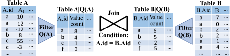
Figure 2. Example of query $Q$ joining two tables with join condition $A.id=B.Aid$ and filter predicates $Q(A)$ and $Q(B)$.

We first illustrate the main idea with a simple example of a two-table join query. Then, we formalize the join query estimation problem as a PGM inference problem over single table distributions.

Two-table join query example: Figure 2 illustrates a query $Q$ joining tables $A$ and $B$ on the inner join condition $A.id=B.Aid$ with base table filter predicates $Q(A)$ and $Q(B)$. Table $A$ first goes through the filter $Q(A)$, resulting in an intermediate table $A|Q(A)$ (records in $A$ that satisfy the filter $Q(A)$). The same procedure is applied to table $B$. Then, the query $Q$ will match the value of join keys $A.id$ and $B.Aid$ from these two intermediate tables. Specifically, the value $a$ appears $8$ times in table $A|Q(A)$ and $6$ times in table $B|Q(B)$, resulting in value $a$ appearing $48$ times in the join result. Therefore, we can calculate the cardinality of this query $Q$ as $8\times 6+4\times 5+3\times 5=83$.

We can formulate the above procedure for calculating $Q$ as a statistical equation in Equation 1, where $D(A.id)$ denotes the domain of all unique values of $A.id$. We observe that only single-table distributions $P_{A}$ and $P_{B}$ are required to accurately compute the cardinality of this join query. Also in this equation, $P_{A}(A.id\!=\!v|Q(A))*|Q(A)|$ equals to $P_{A}(A.id\!=\!v\land Q(A))*|A|$, which is exactly what single-table CardEst methods estimate. Thus, we can accurately calculate the cardinalities of two-table join queries using single-table estimators. Note that the summation over the domain of join key $\mathcal{D}(A.id)$ has the same complexity as computing the join. Therefore, we need to approximate this calculation for FactorJoin to be practical. The details of our approximation schemes are given in Section 3.2 and Section 4.

$$|Q|=\sum_{v\in\mathcal{D}(A.id)} P_{A}(A.id=v|Q(A))*|Q(A)|*$$

(1) $$P_{B}(B.Aid=v|Q(B))*|Q(B)|$$

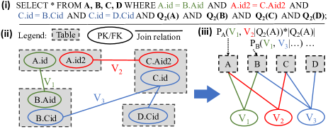
Figure 3. Formulating a join query CardEst into a factor graph inference problem. Figure (i) shows a SQL query $Q_{2}$. Figure (ii) visualizes the join template of $Q_{2}$. Figure (iii) presents the factor graph model to compute $Q_{2}$’s cardinality.

Formal problem formulation: A general join query can involve a combination of different forms of joins (e.g., chain, star, self, or cyclic joins) so its counterpart equation (as Equation 1) can be very difficult to derive and compute; we have put these equations/derivations in the supplementary material. We provide a generalizable formulation that automatically decomposes join queries into single-table estimations using the factor graph model.

Figure 3-(i) shows a SQL query $Q_{2}$ joining four tables $A,B,C,D$. We visualize its join template as a graph in Figure 3-(ii), where each dashed rectangle represents a table, each ellipse (node) represents a join-key in $Q_{2}$, and each solid line (edge) represents an equi-join relation between two join keys connected by it. Note that both sides of an equi-join relation represent the semantically equivalent join keys. We call them equivalent key group variables. In Figure 3-(ii), there are three connected components and thus three equivalent key group variables $V_{1},\ldots,V_{3}$. $V_{1}$ represents $A.id$ and $B.Aid$ in this group since $Q_{2}$ contains the join condition $A.id=B.Aid$.

The exact computation required to compute the cardinality of the SQL query in Figure 3 extends Equation 1 to sum over the domain $\mathcal{D}$ of each join key.

$$|Q_{2}|= \sum_{a1\in\mathcal{D}(A.id)}\ \ \ \ \ \sum_{a2\in\mathcal{D}(A.id2)}\ \ \ \ \ \sum_{c\in\mathcal{D}(C.id)}$$

$$P_{A}(A.id=a1,\ A.id2=a2\ |\ Q_{2}(A))\ast|Q_{2}(A)|$$

$$\ast P_{B}(B.Aid=a1,\ B.Cid=c\ |\ Q_{2}(B))\ast|Q_{2}(B)|$$

$$\ast P_{C}(C.Aid2=a2,\ C.id=c\ |\ Q_{2}(C))\ast|Q_{2}(C)|$$

(2) $$\ast P_{D}(D.Cid=c\ |\ Q_{2}(D))\ast|Q_{2}(D)|$$

This computation is extremely expensive — assuming the domains of each id being $n$, a naive implementation would have the complexity $O(n^{3})$. We can improve this complexity to $O(n^{2})$ by representing this computation as an equivalent factor graph model (Loeliger, 2004), which is a particular class of probabilistic graphical models (PGMs) (Koller and Friedman, 2009). We have $2$ in the exponent because the maximum number of join keys in $Q_{2}$ is two in the table $A$. This is still very expensive, but in Section 3.2, we describe how we can use principled approximations made possible by the factor graph formulation to make the inference complexity practical.

A factor graph is a bipartite graph with two types of nodes: variable nodes, and factor nodes representing an unnormalized probability distribution w.r.t. the variables connected to it. Figure 3-(iii) shows the constructed factor graph $\mathcal{F}$ for computing the cardinality of $Q_{2}$. Specifically, $\mathcal{F}$ contains a variable node for each equivalent key group variable $V_{i}$, and a factor node for each table touched by $Q_{2}$. A factor node is connected to a variable node if the variable represents a key in the table. In this case, the factor node representing table $A$ is connected to $V_{1}$ (equivalent to $A.id$) and $V_{2}$ (equivalent to $A.id2$). Each factor node maintains an unnormalized probability distribution for the variable nodes connected to it, for e.g., node $A$ maintains $P_{A}(V_{1},V_{2}|(Q_{2}(A)))*|Q_{2}(A)|$, which is the same as the distribution $P_{A}(A.id,A.id2|(Q_{2}(A)))*|Q_{2}(A)|$ used in Equation 2. The factor graph model utilizes the graph structure to compute the sum using the well-studied inference algorithms.

We can more formally state this relationship between computing the join cardinalities and factor graphs as the following lemma, whose proof is provided in the supplementary material.

Lemma 0.

Given a join graph $\mathcal{G}$ representing a query $Q$, there exists a factor graph $\mathcal{F}$ such that the variable nodes in $\mathcal{F}$ are the equivalent key group variables of $\mathcal{G}$ and each factor node represents a table $I$ touched by $Q$. A factor node is connected to a variable node if and only if this variable represents a join-key in table $I$. The potential function of a factor node is defined as table $I$’s probability distribution of the connected variables (join keys) conditioned on the filter predicates $Q(I)$. Then, calculating the cardinality of $Q$ is equivalent to computing the partition function of $\mathcal{F}$.

3.2. Inference complexity analysis

Inference on factor graphs is a well-studied problem in the domain of PGMs (MacKay et al., 2003; Koller and Friedman, 2009; Loeliger, 2004). Popular approaches to solving this problem are variable elimination (VE) (Koller and Friedman, 2009) and belief propagation algorithms (Kschischang et al., 2001). In FactorJoin’s implementation, we use the VE, which first determines an optimal order of variables and then sums over the distributions defined by the factor graph model in this order. The complexity of VE is $O(N*|D|^{max(|JK|)})$, where $N$ is the number of equivalent key groups ($3$ in Figure 3), $|D|$ is the largest domain size of all join keys, and $max(|JK|)$ is the maximum number of join keys in a single table ($2$ in Figure 3). Intuitively, this complexity is because the factor nodes need to understand the joint distribution of all join keys in one table. Thus, the largest factor node in the factor graph model maintains a probability distribution of size $|D|^{max(|JK|)}$. This complexity is not practical for real-world queries, as $|D|$ can be millions, and $max(|JK|)$ can be larger than $4$ in real-world DB instances, such as IMDB (Leis et al., 2015). Therefore, instead of calculating the exact cardinality, we propose a new PGM inference algorithm for FactorJoin that can estimate an upper bound on cardinality. Past works (Cai et al., 2019; Atserias et al., 2008; Abo Khamis et al., 2017) have shown that cardinality upper bounds can help avoid very expensive query plans since under-estimating a large result can sometimes be catastrophic. For instance, an optimizer might choose to do a nested loop join if a CardEst method under-estimates that the result would easily fit in memory. This would lead to a disastrous plan if the actual result size is much larger than estimated.

Our approximate inference algorithm performs two approximations: 1) reducing the domain size $|D|$ using binning and 2) decreasing the exponent, $max(|JK|)$, by approximating the distribution of attributes in a single table. Specifically, for binning, we first partition the domain of all join keys into $k$ bins. Instead of summing over the entire domain, we only need to sum over $k$ summarized values (probabilistic bounds) of each bin. The details are provided in Section 4. Second, we approximate the causal relation among all attributes within a table as a tree structure. This allows us to factorize the $max(|JK|)$-dimensional joint distribution of all join keys in a table as a product of two-dimensional conditional distributions. This procedure is known as structure learning in Bayesian networks in the PGM domain (Chow and Liu, 1968). Past work on single table cardinality estimation has shown that such tree approximations do not decrease the modeling accuracy significantly (Wu et al., 2020a). Further details are provided in Section 5.1.

Thereafter, we can directly run the VE inference algorithm on the binned domains and factorized two-dimensional distributions to estimate the cardinality upper bound of $Q$. With these two approximate inference techniques, the complexity of estimating the cardinality bound is reduced to $O(N*k^{2})$, which is very efficient as both $N$ and $k$ are very small in practice.

3.3. Workflow overview

The workflow of FactorJoin contains two phases: offline training and online inference (Figure 4). During the offline phase, our framework analyzes the DB instance, bins the domain of join keys, explores the causal relation, and builds CardEst models for every single table. When a join query $Q$ comes in during the online phase, FactorJoin formulates the estimation of this query as a factor graph involving only single-table distributions, estimates them using (pre-trained) single-table estimators, runs PGM inference, and generates a probabilistic bound for $Q$. We provide the details as follows.

Offline training phase: Given a new DB instance, FactorJoin first analyzes its DB schema and data tables to get all possible join relations between different join-keys. We consider two join-keys to be semantically equivalent if there exists a join relation between them. After identifying all groups of equivalent join-keys, we bin the domains of all join-keys in each group. FactorJoin can also optionally use query workload information to optimize this binning procedure (details provided in Section 4.2). Based on the data tables and the binned domains, we explore the causal relation of these attributes and model them as a tree structure (details are provided in Section 5.1). Then, we build the CardEst models to understand the data distribution of every single table. In principle, any single-table CardEst method that is able to provide conditional distributions can be adapted into FactorJoin. In practice, we implement two methods: traditional random sampling and the learned data-driven BayesCard method (Wu et al., 2020a). The sampling method is extremely flexible to use and can easily support any complex filter predicates with disjunctions, string pattern matching, or any user-defined functions. Alternatively, similar to most data-driven methods, BayesCard can only work with queries filtering numeric and categorical attributes, but BayesCard has been shown to consistently produce accurate, fast, and robust estimations for various data distributions (Wu et al., 2020a). Users of FactorJoin can switch between different single-table estimators based on their objectives and knowledge about the DB instances.

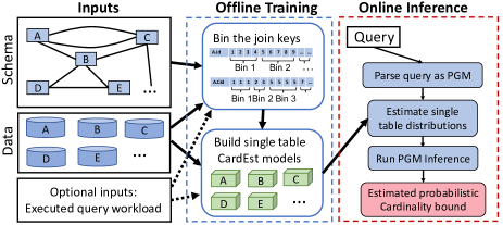
Figure 4. Workflow of FactorJoin framework.

Online inference phase: When a join query $Q$ comes in during run-time, FactorJoin will first parse its join graph and construct the corresponding factor graph $\mathcal{F}$ (as in Figure 2). Then, it uses the trained single-table estimators to estimate the join-key distributions conditioned on the filter predicates of $Q$; FactorJoin will use these distributions in the corresponding factor nodes of $\mathcal{F}$. Finally, we run the approximate version of VE inference algorithms on $\mathcal{F}$ to derive the estimated/probabilistic cardinality bound. We note that the CardEst methods working inside a query optimizer will estimate all sub-plan queries of a target query to decide the best query plan. Since these sub-plan queries contain a large amount of overlapping information, we provide a progressive estimation algorithm to avoid computation redundancy in Section 5.2.

4. Probabilistic bound algorithm

In this section, we design a new probabilistic bound algorithm based on binning to calculate the factor graph inference problem. Specifically, we first explain the main ideas with a two-table join example and formulate the algorithm details within FactorJoin in Section 4.1. Then, we discuss how to optimize the bin selection using data and query information in Section 4.2.

4.1. Algorithm details

As described in Section 3, the main objective of our probabilistic bound-based algorithm is to reduce the domain size of the join keys, i.e., reducing the complexity of summation in Equation 1. Thus, instead of running the inference algorithm over the entire domain, FactorJoin only needs to sum over the binned domain.

Two-table join query example: We use the previous example query $Q$ from Section 2 to illustrate the core idea of our probabilistic upper bound algorithm based on binning. The objective is to estimate an upper bound on $Q$, whose exact computation requires summing over the entire domain of $A.id$ according to Equation 1. Assume that we have a set of $k$ bins $\{bin_{1},\ldots,bin_{k}\}$ partitioning the domain of $A.id$ and we apply this same set of bins to $B.Aid$. We need to make sure that a given value in the domain of $A.id$ and $B.Aid$ will always belong to the bin with the same indexes. Then, Equation 1 can be equivalently written as Equation 3. We can then replace the sum over all values in a bin $bin_{i}$ with a probabilistic bound on $bin_{i}$ to estimate an upper bound for $Q$ as Equation 4.

$$|Q| =\sum_{i=1}^{k}\sum_{v\in bin_{i}} P_{A}(A.Id=v|Q(A))*|Q(A)|*$$

(3) $$P_{B}(B.Aid=v|Q(B))*|Q(B)|$$

(4) $$\lesssim\sum_{i=1}^{k} Probabilistic\_bound(A,B,bin_{i})$$

Motivated by a bound based on the most frequent value (MFV) (Hertzschuch et al., 2021), we use a simple probabilistic bound method to derive $Probabilistic\break\_bound(A,B,bin_{i})$ for a particular bin. Specifically, assuming that value $\{a,b,c,e,f\}$ of $A.id$ and $B.Aid$ are binned into $bin_{1}$ as shown in Figure 5. We know the summation of all values in $bin_{1}$ equals to $8\times 6+4\times 5+3\times 5=83$. This summation has a dominating term of $8\times 6$, because the count of MFV of $bin_{1}$ is $8$ for $A.id$ (denoted as $V^{*}_{1}(A.id)$) and $6$ for $B.Aid$ (denoted as $V^{*}_{1}(B.Aid)$) so each value can appear at most $8\times 6$ times in the denormalized table after the join. Since we know the total count of values in $bin_{1}$ for $A.id$ is $16$, there can be at most $16/8=2$ MFVs. Similarly, there can be at most $4$ MFVs in $bin_{1}$ for $B.Aid$. Therefore, we have the summation of all values in $bin_{1}$ is upper bounded by $min(2,4)\times 8\times 6=96$.

We formally represent the aforementioned procedure in Equation 5, where $V^{*}_{i}(A.id)$ and $P_{A}(A.id\in bin_{i}|Q(A))*|Q(A)|$ are the MFV count and estimated total count of $bin_{i}$ for $A.id$. Our bound is probabilistic because $P_{A}(A.id\in bin_{i}|Q(A))*|Q(A)|$ is estimated with a single table CardEst method, which may have some errors.

$$|Q| \lesssim\sum_{i=1}^{k}min(\frac{P_{A}(A.id\in bin_{i}|Q(A))*|Q(A)|}{V^{*}_{i}(A.id)},$$

(5) $$\frac{P_{B}(B.Aid\in bin_{i}|Q(B))*|Q(B)|}{V^{*}_{i}(B.Aid)})*V^{*}_{i}(A.id)*V^{*}_{i}(B.Aid)$$

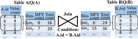
Figure 5. The bound-based algorithm; each bin is summarized by the most frequent value count and total count.

Working with PGM inference: Next, we will explain how to generalize this probabilistic bound to make it work inside the factor graph VE inference algorithm mentioned in Section 2. During the offline training, FactorJoin computes the MFV counts $V^{*}$ for all bins of each join-key. During the online phase, FactorJoin estimates the probability distribution for the binned domain of all join-keys in each table $I$. Then, FactorJoin puts $I$’s distribution $P_{I}$ and MFV counts $V^{*}(I)$ into the corresponding factor node.

Recall that the VE algorithm generates an optimal elimination order of all variables and sums over the domain of these variables sequentially in this order. Since at each step, the variable elimination algorithm sums out only one variable, its probabilistic bound can be derived using Equation 5 over multiple equivalent join keys. Thus, this algorithm does not need to sum over the entire value domain of a variable but can only sum over the probabilistic bounds in the binned domain instead, which greatly reduces the complexity.

Analysis: This probabilistic bound algorithm significantly reduces the domain size of join keys and enables practical approximate PGM inference. Further, this algorithm upper-bounds the cardinality most of the time and the bound is very tight with even a small number of bins, such as $k=100$. Therefore, as we empirically verify in our evaluation, the estimated cardinality bound is very effective.

4.2. Bin selection optimizations

In our probabilistic bound algorithm, different bins can result in drastically different bound tightness. There are two decisions: how many bins to use for each join key group, and what values to put in the same bin.

Deciding $k$ based on query workloads: The number of bins, $k$, has a significant effect on the performance of FactorJoin: fewer bins aggregate more distinct values in the join key domain to each bin and are thus less accurate but more efficient. An approach to tune $k$ is to set different values of $k_{i}$ for different equivalent key groups $Gr_{i}$. Suppose that users provide a budget $K$ with $K=\sum k_{i}$. If FactorJoin has access to the query workload, it can analyze the join patterns and count the number of times $n_{i}$ each $Gr_{i}$ appears in the workload. Our framework can adaptively set a larger $k_{i}$ for the frequently visited $Gr_{i}$ and vice versa. In our implementation, we use a simple heuristic — set $k_{i}=K*n_{i}/\sum_{j}n_{j}$. In this way, we can optimize the modeling capacity of FactorJoin to make sure that it is spent on the important joins.

Binning strategy: For the probabilistic bound algorithm described in Section 4, we observe that the upper bound on a particular bin $bin_{i}$ can be very loose if the MFV count $V^{*}_{i}$ is a large outlier in $bin_{i}$. Taking the two table join query as an example, if $bin_{i}$ contains only one value that appears $100$ times in $A.id$ but $10,000$ values that only appear once in $B.Aid$, then the bound could be $100$ times larger than the actual cardinality. Common binning strategies used in DBMS histograms such as equal-depth or equal-width bins can be catastrophic in such cases. Instead, we want the variance of the join key counts in each bin to be low. This strategy has also been proposed in different contexts (Ioannidis and Christodoulakis, 1991; Ioannidis and Poosala, 1995), but the key challenge is that the same bins will be built for all join keys within an equivalent key group, i.e. join keys that share the same semantics. For example, for a primary key (e.g. “title.id” in IMDB JOB (Leis et al., 2015)), any binning strategy will have zero variance because of uniqueness. However, the same bins will be applied for its equivalent foreign keys (e.g. “movie_id”) on other tables, which may lead to a large variance depending on how often each value repeats in the other tables. We design a greedy binning selection algorithm (GBSA) to optimize for bins with low variance value counts across all tables, as illustrated in Algorithm 2. Jointly minimizing the variance of one bin for all join keys has exponential complexity. Therefore, GBSA uses a greedy algorithm to iteratively minimize the bin variance for all join keys. At a high level, GBSA first optimizes the minimal variance bins with half the binning budget of $k/2$ on the domain of one join key (lines 2-4). Then, it recursively updates these bins by minimizing the variance of other join keys using the other half of the budget (lines 5-13). We put the details of GBSA in the supplementary material.

Discussion: As shown in Section 6.4, GBSA has significantly better performance than naive binning strategies. In the extreme case, if the value counts have zero variance for all equivalent join keys, then our bound can output the exact cardinality. Admittedly, this binning strategy does have the drawback that after applying the filter predicates, the join key frequencies will change and their variance may become higher within a bin. However, we empirically evaluate that for real-world datasets, this phenomenon does not have a severe impact on FactorJoin. In future work, we will explore an enhanced binning strategy that can efficiently address this issue.

Algorithm 1 Greedy Bin Selection Algorithm (GBSA)

Input: Equivalent key groups $Gr_{1},\ldots,Gr_{m}$, where $Gr_{i}=\{Id_{i}^{1},\ldots,Id_{i}^{|Gr_{i}|}\}$;

Column data $\mathcal{D}(Id_{i}^{j})$ of all join keys in the DB instance $\mathcal{D}$;

Number of bins $k_{i}$ for each group $Gr_{i}$.

1:for $Gr_{i}\in\{Gr_{1},\ldots,Gr_{m}\}$ do

2:    $Bin(Gr_{i})\leftarrow$ []

3:    $Gr_{i}^{\prime}\leftarrow sort\_key\_based\_on\_domain\_size(\mathcal{D},Gr_{i})$

4:    $Bin(Gr_{i})\leftarrow get\_min\_variance\_bins(\mathcal{D}(Gr_{i}^{\prime}[1]),k_{i}/2)$

5:    remain_bins $\leftarrow k_{i}/2$

6:    for $j\in\{2,\ldots,|Gr_{i}^{\prime}|\}$ do

7:         binned_data $\leftarrow apply\_bin\_to\_data(\mathcal{D}(Gr_{i}^{\prime}[j]),Bin(Gr_{i}))$

8:         bin_variance $\leftarrow calculate\_variance$(binned_data)

9:         arg_sort_idx $\leftarrow arg\_sort\_decreasing(bin\_variance)$

10:         for $p\in arg\_sort\_idx[1:remain\_bins/2]$ do

11:             $Bin(Gr_{i})\leftarrow min\_variance\_dichotomy(Bin(Gr_{i})[p]$, binned_data[p])

12:         end for

13:         remain_bins $\leftarrow$ remain_bins/2

14:    end for

15:end for

16:return $\{Bin(Gr_{i})|i,\ldots,m\}$

4.3. Incremental model updates

FactorJoin is friendly for DBs with frequent data changes because we only need to incrementally update the single table statistics. In the following, we will discuss the algorithm details in the scenario of data insertion and data deletion can be handled similarly.

Consider we have trained a stale FactorJoin model $\mathcal{F}$ on data $\mathcal{D}$ and would like to incrementally update $\mathcal{F}$ with the inserted data $\mathcal{D}^{\prime}$. FactorJoin needs to identify the inserted tuple values from $\mathcal{D}^{\prime}$ for every join key and put them into the original bins optimized on $\mathcal{D}$. Then, it will update the total and most-frequent value count in each bin. At last, FactorJoin can incrementally update the base table CardEst models with off-the-shelf tools (e.g. BayesCard provides an efficient and effective approach to incrementally update the single-table models using $\mathcal{D}^{\prime}$ (Wu et al., 2020a); materializing a new sample on $\mathcal{D}\bigcup\mathcal{D}^{\prime}$ incrementally updates the sampling-based estimator).

Therefore, the incremental update of FactorJoin does not need to normalize the joined tables nor need to use executed queries. It is also empirically verified to be very efficient and effective. However, during incremental updates, the FactorJoin models keep the same set of bins, which is optimized on the previous data and thus might not be optimal after data insertion. This might cause slight degrade in performance and the user can choose to retrain the model in case of massive data updates.

5. Improving FactorJoin efficiency

We describe two techniques to improve the modeling and estimation efficiency of FactorJoin. First, we model the joint distribution of attributes on a single table as a tree structure and use it to simplify the PGM inference calculations. Next, we define a systematic way of reusing estimates of intermediate sub-plan queries to estimate a larger query. This is only possible because we decompose cardinality estimates into single table sub-components.

5.1. Exploring attributes causal relation

Recall from Section 3.2, the factor graph computation to calculate the cardinality bound is $O(N*k^{max(|JK|)})$, where $N$ is the number of tables, $k$ is the number of bins, and $max(|JK|)$ is the maximum number of join keys in a table. The exponent term, $max(|JK|)$, represents the factor nodes requiring the joint distribution between all join keys on a single table. As $max(|JK|)$ can sometimes be large (e.g., in IMDB it can be up to $4$), we need to reduce the dimensionality of the distributions defined in factor nodes to ensure an efficient CardEst procedure. Fortunately, real-world data has a lot of correlations that can be used to simplify this joint distribution.

Consider a table $A$ with $6$ attributes, $\{id_{1},id_{2},id_{3},id_{4}attr_{1},attr_{2}\}$, four of which are join keys. The factor graph computation may need to estimate quantities such as:

(6) $$P_{A}(id_{1},id_{2},id_{3},id_{4}|Q(A))$$

This requires storing a $4$ dimensional probability distribution, and even with binning the domains of all ids into $k$ bins, it still requires $k^{4}$ space and inference time complexity. This joint distribution can be represented as a graph where each attribute is a node, and there are edges between every pair of attributes. We will use the dependencies and relationships between the attributes and model them as a Bayesian network (BN)  (Koller and Friedman, 2009). Specifically, we will assign each edge in the joint distribution graph a weight proportional to the mutual information between the two attributes connected by the edge. Then, we will remove edges with the least mutual information until only a tree structure graph remains to represent the joint probability over these attributes. This process is known as the Chow-Liu algorithm for decomposing joint distributions (Chow and Liu, 1968). The factorized tree representation of the joint distribution can let us approximate Equation 6 with an equation of the form:

(7) $$P_{A}(id_{1}|Q(A))*P_{A}(id_{2}|Q(A))*P_{A}(id_{3}|id_{1})*P_{A}(id_{4}|id_{3})$$

, which is much more efficient to compute because it only involves a product over at most a two-dimensional distribution. This dimension reduction can cause some errors. But it has been shown empirically that the factorized distributions are accurate approximations of the original distribution for most real-world datasets (Wu et al., 2020a).

Using such an optimization, instead of storing the $max(|JK|)$-dimensional distributions in the factor nodes, the factor graph only needs to store a series of one or two-dimensional data distributions without a significant decrease in estimation accuracy. Therefore, the overall complexity for running approximate inference on this factor graph becomes $O(N*k^{2})$ in both storage and inference speed. Since $k$ is relatively small (around one hundred), estimating one query using FactorJoin is very efficient.

In principle, FactorJoin can also use other methods for the single table distribution inference. This may involve traditional methods, such as sampling, or more powerful graph-structured factorizations of the distributions — which can increase modeling accuracy at the cost of slower estimation speed. Thus, users of FactorJoin can make trade-offs between estimation accuracy and efficiency. We leave exploring these trade-offs as future work.

5.2. Progressive estimates of sub-plan queries

In order to optimize the plan for one query, the CardEst method needs to estimate the cardinalities of hundreds or thousands of sub-plan queries. Estimating all these queries independently is very inefficient because they contain a lot of redundant computation. Similar to the traditional CardEst methods deployed in real DBMSes, FactorJoin supports estimating all sub-plan queries of one query progressively, reusing the computation as much as possible. At a high level, the progressive estimation algorithm will estimate all sub-plan queries in a bottom-up fashion. FactorJoin first estimates all two-table join sub-plan queries, then it estimates the three-table join sub-plan queries, which will contain the two-table joins as their sub-structures, and so on.

Joining Factor Graphs: The key insight is that when we estimate the cardinality of a two-table join, we can also combine their factor graphs into a new factor graph for the joined table. Specifically, as described in Section 3, each base table is represented as a factor node in the factor graph. For instance, the factor node representing $A$ will store the unnormalized probability distribution and the MFV counts for the binned domain of join keys in $A$. When estimating the cardinality of joining $A$ and $C$, our approximate inference algorithm in Equation 5 computes the bound over all bins and sums them. These bounds essentially define an unnormalized probability distribution over all join keys on the denormalized table $A\Join C$. We can derive a bound on the new MFV counts for a join-key $A\Join C$ as the multiplication of the corresponding MFV counts in $A$ and $C$. Therefore, we can cache this new probability distribution and MFV counts in a new factor node representing $A\Join C$. Thus, when estimating the cardinality of $A\Join B\Join C$ we can consider it as a join of two single tables $(A\Join C$) and $B$.

Since all sub-plans can essentially be considered a join of two sub-plans that we have already estimated, our inference algorithm only needs to compute the join of two-factor nodes for each sub-plan query. Therefore, the progressive estimation algorithm has no redundant computation and maximizes efficiency. In experiments, with this algorithm, FactorJoin can estimate the cardinality of $10,000$ sub-plan queries in one second, which is more than ten times faster than estimating all these queries independently. Note that the progressive estimation algorithm is only possible to implement for FactorJoin and the traditional methods because it requires decomposing join queries into single-table estimates. None of the existing learned methods can apply this method since their models are built to model the distributions of specific join patterns.

6. Experimental Evaluation

In this section, we empirically demonstrate the advantages of our framework over existing CardEst methods. We first introduce the datasets, baselines, and experimental environment in Section 6.1. Then, we explore the following questions:

$\bullet$ Overall performance (Section 6.2): how much improvement can FactorJoin achieve in terms of end-to-end query time? What are the model size and training time compared to SOTA methods?

$\bullet$ Detailed analysis (Section 6.3): Why does FactorJoin attain good overall performance? When does it perform better or worse than existing baselines? How will it perform in terms of data updates?

$\bullet$ Ablation study (Section 6.4): How much does each optimization technique of FactorJoin contribute to the overall performance?

6.1. Experimental Setup

Datasets: We evaluate the performance of our CardEst framework on two well-established benchmarks: STATS-CEB (Han et al., 2021) and IMDB-JOB (Leis et al., 2015), whose statistics are summarized in Table 2.

The STATS-CEB benchmark uses the real-world dataset STATS, which is an anonymized dump of user-contributed content on Stack Exchange (Stack Overflow and related websites). This dataset consists of $8$ tables with $34$ columns and more than one million rows. It contains a large number of attribute correlations and skewed data distributions. The STATS-CEB query workload contains $146$ queries involving $70$ different join templates with real-world semantics. The true cardinalities of these queries range from $200$ to $2\cdot 10^{10}$, with some queries taking more than one hour to execute on Postgres. The STATS-CEB benchmark only has star or chain join templates and numerical or categorical filtered attributes — therefore it is possible to evaluate all existing CardEst baselines on it.

The IMDB-JOB benchmark uses the real-world Internet movie database (IMDB). This dataset contains $21$ tables with more than fifty million rows. The IMDB-JOB query workload contains $113$ queries with $33$ different join templates. Some queries have more than $10,000$ sub-plan queries, posing a significant challenge to the efficiency of CardEst methods. Because IMDB-JOB contains cyclic joins and string pattern matching filters, the JoinHist and existing learned data-driven methods do not support this benchmark.

The queries in these two benchmarks cover a wide range of joins, filter predicates, cardinalities, and runtimes. To the best of our knowledge, they represent the most comprehensive and challenging real-world benchmarks for CardEst evaluation.

Baselines: We compare our framework with the most competitive baselines in each CardEst method category.

1) PostgreSQL (Documentation 12, 2020) refers to the histogram-based CardEst method used in PostgreSQL.

2) JoinHist (Dell’Era, 2007) is the classical join-histogram method whose details are explained in Section 2.2.

3) WJSample (Li et al., 2016) uses a random walk based-method called wander join to generate samples from the join of multiple tables. Its superior performance over traditional sampling-based methods has been demonstrated in recent studies (Li et al., 2016; Zhao et al., 2018; Park et al., 2020). We limit the amount of time spent for each random walk of WJSample so the overall time spent for estimating cardinalities is comparable to other methods. If we allow WJSample longer inference time, it can generate more effective query plans — but it is impractical since its total estimation time will exceed the query execution time.

4) MSCN (Kipf et al., 2019) is a learned query-driven method based on a multi-set convolutional network model. On both datasets, we train MSCN on roughly $100K$ sub-plan training queries that have similar distributions to the testing query workloads.

5) BayesCard (Wu et al., 2020a), 6) DeepDB (Hilprecht et al., 2019), and 7) FLAT (Zhu et al., 2021) are the learned data-driven CardEst methods. They use fanout methods to understand the data distributions of all join templates. Then, they apply different distribution models (Bayesian networks, sum-product networks (Poon and Domingos, 2011), factorized sum-product networks (Wu et al., 2020b), respectively) to capture the data distribution on single tables or denormalized join tables. We test these methods on STATS-CEB using the optimally-tuned model parameters, as used in (Han et al., 2021).

8) PessEst (Cai et al., 2019) is the SOTA bound-based method, which leverages randomized hashing and data sketching to tighten the bound for join queries. Its estimation has been verified to be very effective in real-world DBMSes. We use the best-tuned hyperparameters to evaluate PessEst on both benchmarks.

9) U-Block (Hertzschuch et al., 2021) uses top-k statistics to estimate cardinality bounds. The original paper designed a new plan enumeration strategy to work with this bound and showed promising results on IMDB-JOB. However, for a fair comparison, we only evaluate the standalone U-Block CardEst method.

10) TrueCard outputs true cardinality for given queries with no estimation latency. This baseline does not refer to any specific method but represents the optimal CardEst performance.

We omit comparisons with many other CardEst methods (Bruno et al., 2001; Srivastava et al., 2006; Khachatryan et al., 2015; Fuchs et al., 2007; Stillger et al., 2001; Wu et al., 2018; Heimel et al., 2015; Kiefer et al., 2017; Leis et al., 2017; Hasan et al., 2020; Yang et al., 2021; Wu and Cong, 2021; Dutt et al., 2019) because the baselines above have demonstrated clear advantages over these methods in various aspects (Han et al., 2021). In addition, some newly proposed methods (Sun and Li, 2019; Wang et al., 2021; Liu et al., 2021a) do not have open-source implementations yet.

We implemented FactorJoin in Python mainly using the NumPy package. Regarding the hyperparameters of FactorJoin, we assume no knowledge of the query workload and set the bin size $k$ to $100$ for both datasets. We use the BN-based CardEst method (Wu et al., 2020a) as the single-table estimators for STATS-CEB benchmark because this method has been shown to be very accurate, fast, and robust for single-table estimations. For IMDB-JOB, we use random sampling with $1\%$ sampling rate as the single-table estimator because this benchmark contains very complicated filter predicates such as disjunctions and string pattern matching, which are not supported by the learned data-driven methods. We discuss and compare other hyperparameters of our framework in Section 6.4.

Category	Statistics	STATS-CEB	IMDB-JOB
Data	# of tables	8	21
	# of rows in each table	$10^{3}$ — $4\cdot 10^{5}$	6 — $3\cdot 10^{7}$
	# of columns in each table	3 — 10	2-12
	# of join keys	13	36
	# of equivalent key groups	2	11
Query	# of queries	146	113
	# of join templates	70	33
	join template type	star & chain	+cyclic
	# of filter predicates	1 — 16	1 — 13
	filter attributes	numerical & categorical	+string LIKE
	# of sub-plan queries	1 — 75	8 — $1\cdot 10^{4}$
	true cardinality range	200 — $2\cdot 10^{10}$	1 — $4\cdot 10^{6}$
	Postgres runtime (s)	0.05 — $10^{4}$	$5\cdot 10^{-4}$ — 450

Table 2. Summary of STATS-CEB and IMDB-JOB benchmark.

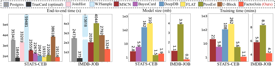
Figure 6. Overall performance on STATS-CEB and IMDB-JOB.

Environment: We use the open-source implementation of all the baselines and tune their parameters to achieve the best possible performance. All experiments are performed on a Ubuntu server with Intel Core Processor CPU with 20 cores, 57GB DDR4 main memory, and 300GB SSD. For end-to-end evaluation, we integrate our framework along with all the baselines into the query optimizer of PostgreSQL 13.1 following the procedure described in the recent work (Han et al., 2021; Han, 2021). We build the primary key and foreign key indices and disable parallel execution in PostgreSQL. Specifically, we inject into PostgreSQL all sub-plan query cardinalities estimated by each method, so the PostgreSQL optimizer uses the injected cardinalities to optimize the query plan, and record the end-to-end query runtime (planning plus execution time). To eliminate the effects of cache, we first execute each workload multiple times. Then, we execute the queries three times for each method and report the average and the standard errors.

6.2. Overall performance

The most straightforward criterion to evaluate the performance of a CardEst method is to test how much each method improves the end-to-end query performance inside the query optimizer. Therefore, we compare the end-to-end performance along with the model size and training time of existing baselines on STATS-CEB and IMDB-JOB.

We summarize the overall performance of all baselines in Figure 6. Recall that JoinHist, BayesCard, DeepDB, and FLAT can not support the IMDB-JOB benchmark. In addition, we do not provide the model size and training time for Postgres, TrueCard, JoinHist, WJSample, and U-Block as they are negligible.

Method	End-to-end time	Exec. + plan time	Improvement
Postgres	35,341s	35,316s + 25s	–
TrueCard (Optimal)	18,456s	18,432s + 24s	47.8%
JoinHist	33,201s	33,173s + 28s	6.1%
WJSample	59,481s	59,436s + 45s	-68.4%
MSCN	25,559s	25,524s + 35s	27.7%
BayesCard	22,679s	22,644s + 35s	35.9%
DeepDB	20,472s	20,304s + 168s	42.0%
FLAT	19,331s	18,934s + 437s	45.3%
PessEst	21,006s	19,872s + 1,135s	40.5%
U-Block	38,618s	38,592s + 26s	-9.3%
FactorJoin (Ours)	19,116s	19,080s + 36s	45.9%

Table 3. End-to-end performance on STATS-CEB.

Performance on STATS-CEB: In addition to Figure 6, we provide a detailed comparison of query execution and planning time (sum over all queries in the STATS-CEB) in Table 3, with the relative end-to-end improvement over Postgres shown in the last column, i.e. (Postgres time - method time) / Postgres time.

FactorJoin achieves the best end-to-end query runtime ($19,116s$), which is close to optimal performance ($18,456s$ for TrueCard). When compared with the traditional methods (Postgres, JoinHist, and WJSample), FactorJoin has significantly better query execution time, indicating that our estimates are much more effective at generating high-quality query plans. Meanwhile, the planning time of our framework is close to Postgres.

Judging from the pure query execution time in Table 3, FactorJoin has comparable estimation effectiveness as the previous SOTA method FLAT on this benchmark. This learned data-driven method uses the fanout method to understand the distribution of all join patterns, which is accurate but very inefficient. Specifically, FactorJoin can achieve better end-to-end performance than FLAT, with $10\times$ smaller planning time, $160\times$ smaller model size, and $240\times$ faster training time. When compared to the other learned methods: BayesCard, DeepDB, and MSCN, FactorJoin can simultaneously achieve better query execution and planning time, smaller model size, and faster training time. Therefore, we empirically verify that instead of modeling the distributions of all join patterns, accurately decomposing the join query into single-table estimates can generate equally effective but more efficient estimation with much smaller model size and training time.

FactorJoin and the SOTA bound-based method PessEst can both generate very effective estimates. This observation verifies that a bound-based method can produce effective estimates because it can help avoid very expensive query plans (Cai et al., 2019; Atserias et al., 2008; Abo Khamis et al., 2017; Han et al., 2021). However, the planning time of PessEst (1135s) is undesirable because it needs to materialize tables after applying the filters and populate the upper bound during run-time. FactorJoin has $35\times$ less planning latency since instead of using exact bounds, we use probabilistic bounds derived from single-table estimates, which is much more efficient.

Method	End-to-end time	Exec. + plan time	Improvement
Postgres	2,472s	2,451s + 21s	–
TrueCard (Optimal)	375s	358s + 17s	84.8%
WJSample	13,618s	12,445s + 1,173s	-450.9%
MSCN	2,039s	1,937s + 102s	18.1%
PessEst	4,044s	1,230s + 2,814s	-63.6%
U-Block	2,792s	2,762s + 30s	-12.9%
FactorJoin (Ours)	1,324s	1,272s + 42s	46.4%

Table 4. End-to-end performance on IMDB-JOB.

Performance on IMDB-JOB: Table 4 shows a detailed end-to-end time comparison for the IMDB-JOB workload.

FactorJoin achieves the best end-to-end query runtime ($1324s$) amongst all baselines. Similar observations hold as in the STATS-CEB workload when compared to the traditional methods. Like STATS-CEB, PessEst achieves the best performance in terms of pure execution time but has a much larger overhead and planning latency. FactorJoin has comparable performance as PessEst in terms of pure execution time. However, our planning time is $50\times$ shorter than PessEst, making our framework much faster in overall end-to-end query time. Specifically, our framework can estimate $10,000$ sub-plan queries within one second, which is close to Postgres.

However, unlike in STATS-CEB where we have near-optimal performance, there still exists a large gap between FactorJoin (1324s) and the optimal TrueCard (375s). There are two possible explanations. First, our probabilistic bound error can accumulate with the number of joins. Compared to STATS-CEB, the IMDB-JOB contains more than twice the number of joins in the queries. Therefore, the relative performance of our framework drops severely when shifting from STATS-CEB to IMDB-JOB. Second, the base-table filters in IMDB-JOB contain a large amount of highly-selective predicates, making our sampling-based single-table CardEst less accurate. These observations suggest room for improving FactorJoin, which we discuss further in the future work section.

Summary: FactorJoin achieves the best performance among all the baselines on both benchmarks. Specifically, FactorJoin is as effective as the previous SOTA methods, and simultaneously as efficient and practical as the traditional CardEst methods.

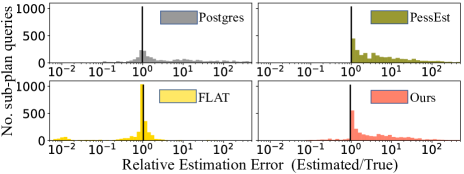
Figure 7. Relative estimation errors on STATS-CEB.

6.3. Detailed Analysis

In this section, we first study why FactorJoin is able to achieve SOTA performance by analyzing the tightness of our probabilistic bound. Then, we exhaustively compare the CardEst method’s end-to-end performance on queries with different runtimes to investigate when can FactorJoin perform better or worse than the competitive baselines. For compactness, here, we only report the results of the most representative methods (Postgres, FLAT, PessEst) on STATS-CEB; the remaining results are in the appendix.

Bound tightness: We show the relative errors between the baselines’ estimates and the true cardinalities (estimate / true) for all sub-plan queries on STATS-CEB in Figure 7. Overall, all three SOTA methods significantly outperform Postgres in terms of estimation accuracy. PessEst generates exact upper bounds and never underestimates. FLAT uses a much larger model to understand the distributions of join patterns and produces the most accurate estimates.

FactorJoin can output an upper bound on cardinality for more than $90\%$ of the sub-plan queries. Most of the marginal underestimates are very close to the true cardinality, which can still generate relatively effective plans. Our generated bounds are slightly tighter than the bounds from PessEst, which explains why our query plans achieve slightly better results.

Detailed comparision: We sort the $146$ queries of STATS-CEB based on their Postgres end-to-end runtime and cluster them into $6$ different runtime intervals. Figure 8 reports relative improvements of the most competitive baselines over Postgres for each query on the left and each cluster of queries on the right.

For the very short-running queries (which represent an OLTP-like workload), Postgres is the best amongst all baselines. These baselines perform worse because the estimation latency plays a significant role in these queries. We observe that improving the estimation accuracy of these queries has a very limited effect on the query plan quality. This also explains why the optimal TrueCard only marginally outperforms Postgres on queries with less than $1s$ of runtime. However, these queries only contribute a negligible proportion of total runtime in STATS-CEB. The query optimizer should fall back to default traditional CardEst methods for OLTP-like workload. FLAT and PessEst are significantly worse than FactorJoin because their planning latency surpasses the execution time, which overshadows the minor improvement in query plans.

For the extremely long-running queries, the advantages of the SOTA methods over Postgres gradually appear. The reason is that estimation latency becomes increasingly insignificant for queries with a long execution time. Thus, FLAT and PessEst which spend a long time planning can generate significantly better query plans. FactorJoin has comparable performance on these queries.

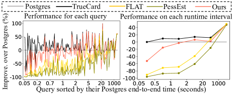
Figure 8. Per query performance of STATS-CEB.

Incremental updates: Following the same evaluation setup as previous work (Han et al., 2021), we train a stale FactorJoin model on STATS data created before 2014 (roughly $50\%$) and insert the rest of the data to incrementally update this model.

We provide the end-to-end query time of the updated FactorJoin and the update time on STATS-CEB queries in Table 5. Since FactorJoin only needs to update single-table statistics, it is extremely efficient, i.e. taking only $2.5s$ to update millions of tuples. This update speed up to $168\times$ faster than the learned data-driven methods with better end-to-end query performance after model update. We cannot fairly compare with the learned query-driven methods because there does not exist a training query workload after the data insertion. It worth noticing that the update times reported for other methods in Table 5 include the time to re-compute the denormalized join tables for the inserted data, so numbers are larger than the ones reported in the original paper (Han et al., 2021).

However, we do see a slight drop in the end-to-end improvement when compared to the FactorJoin trained on the entire dataset ($43.4\%$ in Table 5 versus $45.9\%$ in Table 3). This small performance difference is due to the fact that the bins are decided on the data before 2014 and remain fixed during incremental updates. Therefore, after inserting the new data, the min-variance property of the bins could be violated, resulting in less accurate predictions.

Method	Update time	End-to-end time	Improvement
BayesCard	84s	22,679s	35.9%
DeepDB	310s	21,352s	39.6%
FLAT	422s	22,120s	37.4%
FactorJoin (Ours)	2.5s	20,015s	43.4%

Table 5. Incremental update performance on STATS-CEB.

6.4. Ablation study

We conduct a series of ablation studies to analyze different optimization techniques inside FactorJoin. Specifically, we first investigate how the number of bins (k) affects the overall performance. Next, we analyze the effectiveness of our new bin selection algorithm (GBSA in Section 4.2) over the traditional equal-width and equal-depth algorithms. Then, we study the performance of plugging-in different single-table CardEst methods into FactorJoin. Due to space limitations, we only provide the results on STATS-CEB. At last, we investigate how removing each of the simplifying assumptions improves the performance of the original joining histogram.

Number of bins (k): We train and evaluate FactorJoin with five different number of bins ($1$, $10$, $50$, $100$, $200$). Figure 9 shows the end-to-end query time (A), bound tightness (B), estimation latency per query (C), training time (D), and model size (E) of FactorJoin. For bound tightness, we report the $50\%,95\%,99\%$ percentiles of all queries’ relative error: estimated/true, as the one used in Figure 7.

Figure 9-(A-B) shows that larger numbers of bins ($k$) will generate tighter cardinality bounds and thus more effective query plans. Figure 9-(C-E) shows that more bins also increase estimation latency, training time, and model size, as expected. There are several interesting observations from these results.

$\bullet$ According to Figure 9-(B), with $k=1$ (i.e. bin the entire domain of each join key into one bin) FactorJoin does not generate tight bounds but it still outperforms Postgres baseline by $24.9\%$. This highlights the importance of upper bounds over underestimation and verifies the effectiveness of bound-based algorithms.

$\bullet$ Increasing $k$ can substantially increase the bound tightness. However, at some point (from $k=100$ to $k=200$) the framework stops achieving better end-to-end performance. One explanation is that this fine-grained improvement in estimation accuracy can generate a slightly better query plan but the slower estimation latency cancels out the improvements in query plans.

$\bullet$ The model size increases quadratically with $k$ because FactorJoin has $O(N*k^{2})$ complexity in both storage and inference. However, estimation latency increases linearly with $k$ because the overall inference time is dominated by the single-table CardEst methods’ inference time, whose complexity is linear with $k$.

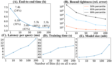
Figure 9. Performance for different number of bins.

Algorithm	End-to-end time	Improvement	Bound Tightness (rel. error)
			50%	95%	99%
Equal-width	23,868s	32.4%	8.7	3,135	$2\times 10^{5}$
Equal-depth	23,436s	33.6%	8.4	2,050	$7\times 10^{4}$
GBSA	19,116s	45.9%	3.3	44	2,782

Table 6. Performance of different binning techniques.

Different bin selection algorithms: Recall that in Section 4.2, we design a new algorithm (GBSA) to optimize the binning process for FactorJoin. Here, we compare it with the traditional equal-width and equal-depth binning algorithms. We set $k=100$ for all three algorithms. They have approximately the same estimation latency, training time, and model size. Thus, we only report the end-to-end performance and bound tightness in Figure 6. We observe that GBSA generates much tighter upper bounds, leading to significantly better end-to-end performance. This demonstrates the effectiveness of our GBSA algorithm.

Varying single-table CardEst methods: To compare the importance of different single-table CardEst methods in FactorJoin, we tried three different estimators: 1) Bayesian network (BayesCard) for single-table, which is the SOTA learned single-table method (Wu et al., 2020a), 2) Sampling, which draws a random sample (5%) from single tables on-the-fly and estimates the cardinalities of filter predicates, and 3) TrueScan which scans and filters the tables during query time and calculate the true cardinalities. The end-to-end performance of different single table estimators with bin size $k=100$ is shown in Table 7. The BayesCard method performs significantly better than Sampling because of more accurate estimates and slightly faster estimation speeds. TrueScan produces an exact upper bound on the cardinalities and thus generates more effective query plans. However, the estimation latency is too high, making its overall end-to-end performance worse than BayesCard.

Method	End-to-end time	Exec. + plan time	Improvement
BayesCard	19,116s	19,080s + 36s	45.9%
Sampling	20,633s	20,592s+ 41s	41.6%
TrueScan	19,334s	18,756s + 578s	45.3%

Table 7. FactorJoin, varying single-table CardEst methods.

Improvement over joining histograms: Since FactorJoin follows the convention of JoinHist, we investigate how much each component of FactorJoin help improve this method. Specifically, apart from the original JoinHist method, we evaluate and compare the following variants. We incorporate our new probabilistic bound into JoinHist to remove its join uniformity assumption (denote as with Bound). We incorporate into JoinHist the histograms learned from BayesNet that represent conditional distributions of join keys given the filter predicates (denote as with Conditional). This variant avoids the attribute independent assumption. FactorJoin reduces to the JoinHist with both bound and conditional techniques on non-cyclic join templates. The results in Table 8 demonstrate that we can achieve significant improvement over the JoinHist method by removing either or all of its simplifying assumptions.

Summary: With a reasonable bin size $k$, FactorJoin generates tight bounds and effective query plans. The GBSA bin selection algorithm is very effective at generating high-quality plans. Single-table estimators do have an impact on FactorJoin’s overall performance and we should choose one that can generate effective and efficient estimates. Overall, all different settings/hyperparameters of FactorJoin can significantly outperform Postgres as well as all existing SOTA methods, demonstrating the robustness and stability of FactorJoin.

Method	End-to-end time	Exec. + plan time	Improvement
JoinHist	33,201s	33,173s + 28s	6.1%
with Bound	29,175s	29147s+ 28s	17.46%
with Conditional	23,450s	23,414s + 36s	31.7%
with Both (Ours)	19,116s	19,080s + 36s	45.9%

Table 8. Performance comparison with JoinHist.

7. Related work

We briefly review literatures on single-table CardEst methods and the learned query optimizers.

Single-table CardEst: Machine learning approaches have been use to solve single-table CardEst problem, which can achieve accurate estimation with very low latency and overhead (Yang et al., 2019; Wu et al., 2020a; Zhu et al., 2021). Specifically, the data-driven learned methods build statistical models to understand data distributions, such as deep autoregressive models (Yang et al., 2019; Hasan et al., 2019), Bayesian networks (Wu et al., 2020a; Halford et al., 2019; Getoor et al., 2001), sum-product-networks (Hilprecht et al., 2019), factorized sum-product-networks (Zhu et al., 2021), and normalizing flow models (Wang et al., 2021). As for the query-driven methods, the first approach using neural networks for CardEst has been proposed for UDF predicates (Lakshmi and Zhou, 1998). Later on, a semi-automatic alternative (Malik et al., 2007) and a regression-based model (Akdere et al., 2012) were used for general predicates. Recently, more sophisticated supervised models such as multi-set convolutional networks (Kipf et al., 2019), XG-boost (Dutt et al., 2019), tree-LSTM (Sun and Li, 2019), and deep ensembles (Liu et al., 2021a), are used to provide accurate estimation.

These works are orthogonal to our framework and in principle, we can support plugging in any one of them for single table CardEst.

Learned query optimizer: Apart from CardEst, there exist a large number of works that use ML to solve other tasks of query optimizer, such as cost estimation and join order selection. Learned cost estimation methods use tree convolution (Marcus and Papaemmanouil, 2019) and tree-LSTM (Sun and Li, 2019) to encode a query plan as a tree and map the encoding to its estimated costs. Active learning (Ma et al., 2020) and zero-shot learning (Hilprecht and Binnig, 2022) are proposed to tackle this problem from a new perspective. Some deep reinforcement learning approaches (Yu et al., 2020; Marcus and Papaemmanouil, 2018) have been proposed to determine the optimal join order. Recently, many methods (Marcus et al., 2019, 2021; Negi et al., 2021a; Wu et al., 2022) propose to learn the entire query optimizer end-to-end without a clear separation of these components.

8. Conclusions

In this paper, we propose FactorJoin, a framework for cardinality estimation of join queries. It combines classical join-histogram methods with learned single table cardinality estimates into a factor graph model. This framework converts CardEst problem into an inference problem over the factor graph involving only single-table distributions. We further propose several optimizations to make this problem tractable for large join graphs. Our experiments show that FactorJoin generates effective and efficient estimates and is suitable for system deployment on large real-world join benchmarks. Specifically, FactorJoin produces more effective estimates than the previous SOTA learned methods, with 40x less estimation latency, 100x smaller model size, 100x faster updating speed, and 100x faster training speed, while matching or exceeding them in terms of query execution time. We believe this work points out a new direction for estimating join queries, which would enable truly practical learned CardEst methods as a system component.

Appendix A Equations and proofs

A.1. Equations for decomposing joins into single-tables

In this section, we provide the case-by-case equations on how to accurately formulate join estimation problem into single-table CardEst problem without any simplified assumptions.

Two-table join case:

Assume that we have two tables $A$ and $B$ with join keys $A.id$ and $B.Aid$ and a query $Q=Q(A)\mathbin{\rule[0.6458pt]{2.20001pt}{0.6pt}\hbox to0.0pt{\hss\rule[3.87495pt]{2.20001pt}{0.6pt}}\mkern-5.5mu\bowtie\mkern-5.5mu\rule[0.6458pt]{2.20001pt}{0.6pt}\hbox to0.0pt{\hss\rule[3.87495pt]{2.20001pt}{0.6pt}}}Q(B)$ where $Q(A)$ is the filter on table $A$ and same for $Q(B)$. The join condition is $A.id=B.Aid$. Then, the join cardinality of $Q$ can be expressed as follows where $D(A.id)$ represents the domain of $A$.

$$|Q|=\sum_{v\in D(A.id)} P_{A}(A.id=v|Q(A))*|Q(A)|*$$

(8) $$P_{B}(B.Aid=v|Q(B))*|Q(B)|$$

Chain join cases:

Case1 A.id = B.Aid = C.Aid: Assume we have three tables $A$, $B$ and $C$ with join keys $A.id$, $B.Aid$, and $C.Aid$. There exists query $Q=Q(A)\mathbin{\rule[0.6458pt]{2.20001pt}{0.6pt}\hbox to0.0pt{\hss\rule[3.87495pt]{2.20001pt}{0.6pt}}\mkern-5.5mu\bowtie\mkern-5.5mu\rule[0.6458pt]{2.20001pt}{0.6pt}\hbox to0.0pt{\hss\rule[3.87495pt]{2.20001pt}{0.6pt}}}Q(B)\mathbin{\rule[0.6458pt]{2.20001pt}{0.6pt}\hbox to0.0pt{\hss\rule[3.87495pt]{2.20001pt}{0.6pt}}\mkern-5.5mu\bowtie\mkern-5.5mu\rule[0.6458pt]{2.20001pt}{0.6pt}\hbox to0.0pt{\hss\rule[3.87495pt]{2.20001pt}{0.6pt}}}Q(C)$ on join condition $A.id=B.Aid\ \ \text{AND}\ \ B.Aid=C.Aid$. Then, the join cardinality can be expressed as follows:

$$|Q| =\sum_{v\in D(A.id)}P_{A}(A.id=v|Q(A))*|Q(A)|*$$

(9) $$P_{B}(B.Aid=v|Q(B))*|Q(B)|*P_{C}(C.Aid=v|Q(C))*|Q(C)|$$

Case2 A.id = B.Aid, B.id = C.Bid: Assume we have three tables $A$, $B$ and $C$ with join keys $A.id$, $B.Aid$, $B.id$, and $C.Bid$. There exists query $Q=Q(A)\mathbin{\rule[0.6458pt]{2.20001pt}{0.6pt}\hbox to0.0pt{\hss\rule[3.87495pt]{2.20001pt}{0.6pt}}\mkern-5.5mu\bowtie\mkern-5.5mu\rule[0.6458pt]{2.20001pt}{0.6pt}\hbox to0.0pt{\hss\rule[3.87495pt]{2.20001pt}{0.6pt}}}Q(B)\mathbin{\rule[0.6458pt]{2.20001pt}{0.6pt}\hbox to0.0pt{\hss\rule[3.87495pt]{2.20001pt}{0.6pt}}\mkern-5.5mu\bowtie\mkern-5.5mu\rule[0.6458pt]{2.20001pt}{0.6pt}\hbox to0.0pt{\hss\rule[3.87495pt]{2.20001pt}{0.6pt}}}Q(C)$ on join condition $A.id=B.Aid\ \ \text{AND}\ \ B.id=C.Bid$. Then, the join cardinality can be expressed as follows:

$$|Q|= \sum_{v_{1}\in D(A.id)}\sum_{v_{2}\in D(B.id)}P_{A}(A.id=v_{1}|Q(A))*|Q(A)|*$$

$$P_{B}(B.Aid=v_{1},B.id=v_{2}|Q(B))*|Q(B)|*$$

(10) $$P_{C}(C.Bid=v_{2}|Q(C))*|Q(C)|$$

Self join case:

Assume we have one table $A$ with join keys $A.id,A.id_{2}$. There exists a query $Q=Q(A)\mathbin{\rule[0.6458pt]{2.20001pt}{0.6pt}\hbox to0.0pt{\hss\rule[3.87495pt]{2.20001pt}{0.6pt}}\mkern-5.5mu\bowtie\mkern-5.5mu\rule[0.6458pt]{2.20001pt}{0.6pt}\hbox to0.0pt{\hss\rule[3.87495pt]{2.20001pt}{0.6pt}}}Q(A^{\prime})$ on join condition $A.id=A.id_{2}$. Then, the join cardinality can be expressed as follows:

$$|Q|=\sum_{v\in D(A.id)} P_{A}(A.id=v|Q(A))*|Q(A)|*$$

(11) $$P_{A}(A.id_{2}=v|Q(A^{\prime}))*|Q(A^{\prime})|$$

Cyclic join case:

Assume we have two tables $A$ and $B$ with join keys $A.id,A.id_{2}$ and $B.Aid,B.Aid_{2}$. There exists a query $Q=Q(A)\mathbin{\rule[0.6458pt]{2.20001pt}{0.6pt}\hbox to0.0pt{\hss\rule[3.87495pt]{2.20001pt}{0.6pt}}\mkern-5.5mu\bowtie\mkern-5.5mu\rule[0.6458pt]{2.20001pt}{0.6pt}\hbox to0.0pt{\hss\rule[3.87495pt]{2.20001pt}{0.6pt}}}Q(B)$ on join condition $A.id=B.Aid\ \ \text{AND}\ \ A.id_{2}=B.Aid_{2}$. Then, the join cardinality can be expressed as follows:

$$|Q|= \sum_{v_{1}\in D(A.id)}\sum_{v_{2}\in D(A.id_{2})}P_{A}(A.id=v_{1}|Q(A))*|Q(A)|*$$

$$P_{B}(B.Aid=v_{1},B.Aid_{2}=v_{2}|Q(B))*|Q(B)|*$$

$$P_{A}(A.id_{2}=v_{2}|Q(A^{\prime}))*|Q(A^{\prime})|$$

$$= \sum_{v_{1}\in D(A.id)}\sum_{v_{2}\in D(A.id_{2})}P_{B}(B.Aid=v_{1}|Q(B))*|Q(B)|$$

$$P_{A}(A.id=v_{1},A.id_{2}=v_{2}|Q(A))*|Q(A)|*$$

(12) $$P_{B}(B.Aid_{2}=v_{2}|Q(B^{\prime}))*|Q(B^{\prime})|$$

A.2. Proof of lamma 1

Lemma 0.

Given a join graph $\mathcal{G}$ representing a query $Q$, there exists a factor graph $\mathcal{F}$ such that the variable nodes in $\mathcal{F}$ are the equivalent key group variables of $\mathcal{G}$ and each factor node represents a table $I$ touched by $Q$. A factor node is connected to a variable node if and only if this variable represents a join key in table $I$. The potential function of a factor node is defined as table $I$’s probability distribution of the connected variables (join keys) conditioned on the filter predicates $Q(I)$. Then, calculating the cardinality of $Q$ is equivalent to computing the partition function of $\mathcal{F}$.

Proof: Assume that we have a query $Q$ joining $m$ tables $A,B,\ldots,M$. We represent $Q$ as a join graph $G$, where each node represents a join key and each edge represents a join relation between two keys connected by it. We further define hyper-nodes in $G$ as a set of nodes whose corresponding join key lies in the same table. Thus, each hyper-nodes naturally represents a table in $Q$. A visualization of such $G$ can be found in Figure 3. Each connected components of $G$ connects a group of join keys with equal join relation, suggesting that they share the same semantics. Therefore, we consider all join keys in a connected component as a equivalent key group variable, denoted as $V_{i}$. Therefore, $G$ defines $n$ equivalent variables $V_{1},\ldots,V_{n}$.

Then, assume that we have a set of unnormalized single table distributions $P_{A}(V_{A}|Q(A))*|Q(A)|,\ldots,P_{M}(V_{M}|Q(M))*|Q(M)|$ and $P_{A}(V_{A^{\prime}}|Q(A^{\prime}))*|Q(A^{\prime})|,\ldots,P_{M}(V_{M^{\prime}}|Q(M^{\prime}))*|Q(M^{\prime})|$. Each $V_{I}$ presents a set of equivalent variables that represent a join key in table $I$. The $I^{\prime}$ is the duplicated table introduced by query $Q$ only if there exists a cyclic join situation. Therefore, the cardinality of $Q$ can be writen as:

$$|Q|= \sum_{v_{1}\in D(V_{1})}\sum_{v_{2}\in D(V_{2})}\cdots\sum_{v_{n}\in D(V_{n})}(P_{A}(V_{A}|Q(A))*|Q(A)|)*$$

$$(P_{B}(V_{B}|Q(B))*|Q(B)|)*\cdots(P_{M}(V_{M}|Q(M))*|Q(M)|)*$$

(13) $$(P_{A}(V_{A^{\prime}}|Q(A^{\prime}))*|Q(A^{\prime})|)*\cdots(P_{M^{\prime}}(V_{M^{\prime}}|Q(M^{\prime}))*|Q(M^{\prime})|)$$

Next, let’s construct a factor graph $\mathcal{F}$, such that the variable nodes in $\mathcal{F}$ are the equivalent key group variables $V_{i}$ of $\mathcal{G}$ and the factor nodes in $\mathcal{F}$ represent the tables $A,\ldots,M$ touched by $Q$ and the duplicated tables if exist $A^{\prime},\ldots,M^{\prime}$. A factor node representing table $I$ is connected to a variable node if and only if this variable represents a join key in table $I$. The potential function of a factor node is defined as the unnormalized probability distribution $P_{I}(V_{I}|Q(I))*|Q(I)|$. The partition function of $\mathcal{F}$ is defined exactly the same as Equation A.2. Therefore, instead of summing a nested loop of $n$ variables $V_{i}$ by brute-force, the partition function (cardinality) can be computed using the well-established variable elimination and belief propogation techniques in PGM domain.

A.3. Probabilistic bound

FactorJoin approximate the exact cardinality computation with a probabilistic bound based inference algorithm. An example on two table join queries can found below. In this section we discuss how to derive an upper bound ($Probabilistic\_bound(A,B,bin_{i})$ in this equation) for different case of join.

$$|Q| =\sum_{i=1}^{k}\sum_{v\in bin_{i}} P_{A}(A.Id=v|Q(A))*|Q(A)|*$$

$$P_{B}(B.Aid=v|Q(B))*|Q(B)|$$

(14) $$\lesssim\sum_{i=1}^{k} Probabilistic\_bound(A,B,bin_{i})$$

Case1: Joining two tables$A.id=B.Aid$:

Let $V_{i}^{*}(A.id)=MAX_{v\in bin_{i}}|A.id=v|$ be the most frequent value (MFV) count of $A.id$ in a bin $bin_{i}$, and same for $V_{i}^{*}(B.Aid)$. We have the following bound:

$$|Q| =\sum_{v=D(A.id)} P_{A}(A.Id=v|Q(A))*|Q(A)|*$$

$$P_{B}(B.Aid=v|Q(B))*|Q(B)|$$

$$\leq\sum_{i=1}^{k}min( \frac{P_{A}(A.id\in bin_{i}|Q(A))*|Q(A)|}{V^{*}_{i}(A.id)},$$

$$\frac{P_{B}(B.Aid\in bin_{i}|Q(B))*|Q(B)|}{V^{*}_{i}(B.Aid)})*$$

(15) $$V^{*}_{i}(A.id)*V^{*}_{i}(B.Aid)$$

Case2: Joining three tables $A.id=B.Aid=C.Aid$:

Let $V_{i}^{*}(A.id)=MAX_{v\in bin_{i}}|A.id=v|$ be the most frequent value (MFV) count of $A.id$ in a bin $bin_{i}$, and same for $V_{i}^{*}(B.Aid)$, $V_{i}^{*}(C.Aid)$. We have the following bound:

$$|Q| =\sum_{v\in D(A.id)}P_{A}(A.id=v|Q(A))*|Q(A)|*$$

$$\hskip 20.00003ptP_{B}(B.Aid=v|Q(B))*|Q(B)|*P_{C}(C.Aid=v|Q(C))*|Q(C)|$$

$$\leq\sum_{i=1}^{k}min\{\frac{P_{A}(A.id\in bin_{i}|Q(A))*|Q(A)|}{V_{i}^{*}(A.id)},$$

$$\hskip 50.00008pt\frac{P_{B}(B.Aid\in bin_{i}|Q(B))*|Q(B)|}{V_{i}^{*}(B.Aid)}$$

$$\hskip 50.00008pt\frac{P_{C}(C.Aid\in bin_{i}|Q(C))*|Q(C)|}{V_{i}^{*}(C.Aid)}\}*$$

(16) $$\hskip 50.00008pt{V_{i}^{*}(A.id)}*{V_{i}^{*}(B.Aid)}*{V_{i}^{*}(C.Aid)}$$

Case3: Joining three tables $A.id=B.Aid$, $B.id=C.Bid$:

Let $V_{i}^{*}(A.id)=MAX_{v\in bin_{i}}|A.id=v|$ be the most frequent value (MFV) count of $A.id$ in a bin $bin_{i}$, and same for $V_{i}^{*}(B.Aid)$, $V_{i}^{*}(B.id)$, and $V_{i}^{*}(C.Bid)$. We have the following bound, where $Upper(A\mathbin{\rule[0.6458pt]{2.20001pt}{0.6pt}\hbox to0.0pt{\hss\rule[3.87495pt]{2.20001pt}{0.6pt}}\mkern-5.5mu\bowtie\mkern-5.5mu\rule[0.6458pt]{2.20001pt}{0.6pt}\hbox to0.0pt{\hss\rule[3.87495pt]{2.20001pt}{0.6pt}}}B)$ is derived from Equation 15.

$$|Q| =\sum_{v_{1}\in D(A.id)}\sum_{v_{2}\in D(B.id)}P_{A}(A.id=v_{1}|Q(A))*|Q(A)|*$$

$$\hskip 60.00009ptP_{B}(B.Aid=v_{1},B.id=v_{2}|Q(B))*|Q(B)|*$$

$$\hskip 60.00009ptP_{C}(C.Bid=v_{2}|Q(C))*|Q(C)|$$

$$\leq\sum_{i=1}^{k}min\{\frac{Upper(Q(A)\mathbin{\rule[0.6458pt]{2.20001pt}{0.6pt}\hbox to0.0pt{\hss\rule[3.87495pt]{2.20001pt}{0.6pt}}\mkern-5.5mu\bowtie\mkern-5.5mu\rule[0.6458pt]{2.20001pt}{0.6pt}\hbox to0.0pt{\hss\rule[3.87495pt]{2.20001pt}{0.6pt}}}Q(B))}{V_{i}^{*}(A.id)*V_{i}^{*}(B.id)},$$

$$\hskip 50.00008pt\frac{P_{C}(C.Aid\in bin_{i}|Q(C))*|Q(C)|}{V_{i}^{*}(C.Bid)}\}*$$

(17) $$\hskip 50.00008pt*V_{i}^{*}(A.id)*V_{i}^{*}(B.id)*{V_{i}^{*}(C.Bid)}$$

Case4: Self join of one table $A.id=A.id2$:

Let $V_{i}^{*}(A.id)=MAX_{v\in bin_{i}}|A.id=v|$ be the most frequent value (MFV) count of $A.id$ in a bin $bin_{i}$, and same for $V_{i}^{*}(A.id_{2})$. We have the following bound:

$$|Q| =\sum_{v=D(A.id)} P_{A}(A.Id=v|Q(A))*|Q(A)|*$$

$$P_{A}(A.id_{2}=v|Q(A^{\prime}))*|Q(A^{\prime})|$$

$$\leq\sum_{i=1}^{k}min( \frac{P_{A}(A.id\in bin_{i}|Q(A))*|Q(A)|}{V^{*}_{i}(A.id)},$$

$$\frac{P_{A}(A.id_{2}\in bin_{i}|Q(A^{\prime}))*|Q(A^{\prime})|}{V^{*}_{i}(A.id_{2})})*$$

(18) $$V^{*}_{i}(A.id)*V^{*}_{i}(A.id_{2})$$

Case5: Cyclic join of two tables $A.id=B.Aid$, $A.id_{2}=B.Aid_{2}$:

Let $V_{i}^{*}(A.id)=MAX_{v\in bin_{i}}|A.id=v|$ be the most frequent value (MFV) count of $A.id$ in a bin $bin_{i}$, and same for $V_{i}^{*}(B.Aid)$, $V_{i}^{*}(A.id_{2})$, and $V_{i}^{*}(B.Aid_{2})$. We have the following bound:

$$|Q| =\sum_{v_{1}\in D(A.id)}\sum_{v_{2}\in D(A.id_{2})}P_{A}(A.id=v_{1},A.id_{2}=v_{2}|Q(A))*$$

$$\hskip 30.00005pt|Q(A)|*P_{B}(B.Aid=v_{1},B.Aid_{2}=v_{2}|Q(B))*|Q(B)|*$$

$$\hskip 30.00005ptP_{A}(A.id_{2}=v_{2}|Q(A^{\prime}))*|Q(A^{\prime})|$$

$$\leq\sum_{i=1}^{k}min\{\frac{Upper(Q(A)\mathbin{\rule[0.6458pt]{2.20001pt}{0.6pt}\hbox to0.0pt{\hss\rule[3.87495pt]{2.20001pt}{0.6pt}}\mkern-5.5mu\bowtie\mkern-5.5mu\rule[0.6458pt]{2.20001pt}{0.6pt}\hbox to0.0pt{\hss\rule[3.87495pt]{2.20001pt}{0.6pt}}}Q(B)}{V_{i}^{*}(A.id_{2})*V_{i}^{*}(B.Aid)},\frac{Upper(Q(A^{\prime})\mathbin{\rule[0.6458pt]{2.20001pt}{0.6pt}\hbox to0.0pt{\hss\rule[3.87495pt]{2.20001pt}{0.6pt}}\mkern-5.5mu\bowtie\mkern-5.5mu\rule[0.6458pt]{2.20001pt}{0.6pt}\hbox to0.0pt{\hss\rule[3.87495pt]{2.20001pt}{0.6pt}}}Q(B))}{V_{i}^{*}(A.id)*V_{i}^{*}(B.Aid_{2})}\}*$$

(19) $$\hskip 50.00008ptV_{i}^{*}(A.id_{2})*V_{i}^{*}(B.Aid)*V_{i}^{*}(A.id)*V_{i}^{*}(B.Aid_{2})$$

Appendix B Greedy bin selection Algorithm details

We observe that the bound on a particular bin $bin_{i}$ can be very loose if the MFV count $V^{*}_{i}$ is a large outlier in $bin_{i}$. Taking the two table join query as an example, if $bin_{i}$ contains only one value that appears $100$ times in $A.id$ but $10,000$ values that only appear once in $B.Aid$, then the bound could be $100$ times larger than the actual cardinality. The existing equal-width or equal-depth binning strategy can generate very large estimation errors, so we design a new binning strategy called the greedy bin selection algorithm (GBSA) to optimize our bound tightness.

The objective of GBSA is to minimize the variance of the value counts within $bin_{i}$. In the extreme case, if the value counts have zero variance for all join keys in one equivalent key group, then our bound can output the exact cardinality (if with perfect single table CardEst models). However, as the same bin partition will be applied for all equivalent join keys, minimizing the value counts variance of $bin_{i}$ on the domain of one key may result in a bad bin for other keys. Jointly minimizing the variance of one bin for all join keys has exponential complexity. There, GBSA uses a greedy algorithm to iteratively minimize the bin variance for all join keys. At a high level, GBSA first optimizes the minimal variance bins with half number of binning budget $k/2$ on the domain of one join key. Then, it recursively updates these bins by minimizing the variance of other join keys using the rest half of the budget. The details of GBSA are provided in Algorithm 2.

Algorithm 2 Greedy Bin Selection Algorithm (GBSA)

Input: Equivalent key groups $Gr_{1},\ldots,Gr_{m}$, where $Gr_{i}=\{Id_{i}^{1},\ldots,Id_{i}^{|Gr_{i}|}\}$;

Column data $\mathcal{D}(Id_{i}^{j})$ of all join keys in the DB instance $\mathcal{D}$;

Number of bins $k_{i}$ for each group $Gr_{i}$.

1:for $Gr_{i}\in\{Gr_{1},\ldots,Gr_{m}\}$ do

2:    $Bin(Gr_{i})\leftarrow$ []

3:    $Gr_{i}^{\prime}\leftarrow sort\_key\_based\_on\_domain\_size(\mathcal{D},Gr_{i})$

4:    $Bin(Gr_{i})\leftarrow get\_min\_variance\_bins(\mathcal{D}(Gr_{i}^{\prime}[1]),k_{i}/2)$

5:    remain_bins $\leftarrow k_{i}/2$

6:    for $j\in\{2,\ldots,|Gr_{i}^{\prime}|\}$ do

7:         binned_data $\leftarrow apply\_bin\_to\_data(\mathcal{D}(Gr_{i}^{\prime}[j]),Bin(Gr_{i}))$

8:         bin_variance $\leftarrow calculate\_variance$(binned_data)

9:         arg_sort_idx $\leftarrow arg\_sort\_decreasing(bin\_variance)$

10:         for $p\in arg\_sort\_idx[1:remain\_bins/2]$ do

11:             $Bin(Gr_{i})\leftarrow min\_variance\_dichotomy(Bin(Gr_{i})[p]$, binned_data[p])

12:         end for

13:         remain_bins $\leftarrow$ remain_bins/2

14:    end for

15:end for

16:return $\{Bin(Gr_{i})|i,\ldots,m\}$

FactorJoin analyzes the schema of DB instance $\mathcal{D}$ to derive $m$ equivalent key groups $Gr_{1},\ldots,Gr_{m}$, each of which contains $|Gr_{i}|$ join keys $Id_{i}^{1},\ldots,Id_{i}^{|Gr_{i}|}$. Let $\mathcal{D}(Id_{i}^{j})$ represents the column data (domain) of join key $Id_{i}^{j}$. GBSA will derive the sub-optimal binning with $k_{i}$ bins $Bin(Gr_{i})=\{bin_{1},\ldots,bin_{k_{i}}\}$ for each the equivalent key group $Gr_{i}$ (line 1). We explain the procedure of this algorithm for binning one group $Gr_{i}$ (line 2-14).

First, GBSA sorts the join keys $\{d_{i}^{1},\ldots,Id_{i}^{|Gr_{i}|}\}$ in decreasing order based on their domain size (line 3) to get $Gr_{i}^{\prime}=\{Id_{i}^{1^{\prime}},\ldots,Id_{i}^{|Gr_{i}|^{\prime}}\}$. We apply half of the binning budget to generate $k_{i}/2$ minimal variance bins on the domain of $d_{i}^{1^{\prime}}$ (line 4). Note that minimal variance bins on a single attribute can be easily obtained by sorting the value counts of $\mathcal{D}(d_{i}^{1^{\prime}})$ and applying equal-depth binning over the sorted values. The remaining number of bins available $remain_{b}ins$ is $k_{i}/2$ (line 5). Then for each rest of the join key $d_{i}^{j}$, GBSA applies the current bins $Bin(Gr_{i})$ to its data column $\mathcal{D}(d_{i}^{j})$, calculates the variance for each bin, and sorts these bins in decreasing order (line 6-9). For the top $remain_{b}ins/2$ bins with the largest variance, we dichotomize each bin into two bins to minimize the variance on join key $d_{i}^{j}$ (lines 10 -12). We iterative the above procedure until all join keys are optimized.

According to our evaluation results, the GBSA has a significant impact on improving our probabilistic bound tightness and estimation effectiveness.

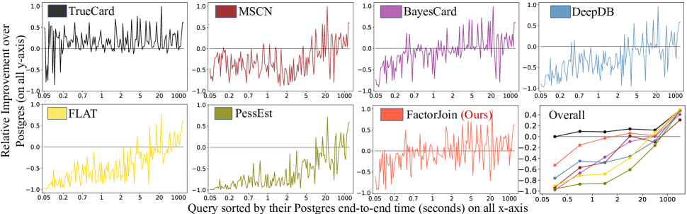
Figure 10. Per query performance of STATS-CEB.

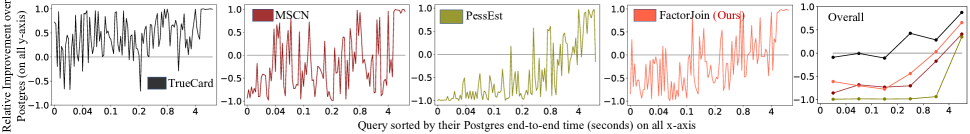
Figure 11. Per query performance of STATS-CEB.

Appendix C Additional experiments and details

In this section, we provide the detailed comparision of all baselines on STATS-CEB and IMDB-JOB benchmarks.

Performance on STATS-CEB: We sort the $146$ queries of STATS-CEB based on their Postgres end-to-end runtime and cluster them into $6$ different runtime intervals. Figure 10 reports relative improvements of all competitive baselines over Postgres for each query and the overall performance comparision on each cluster of queries on the last figure.

For the very short-running queries (which represent an OLTP-like workload), Postgres is the best among all baselines. These baselines perform worse because the estimation latency plays a significant role in these queries. We observe that improving estimation accuracy has a very limited effect on the query plan quality of short-running queries. This also explains why the optimal TrueCard only marginally outperforms Postgres on queries with less than $2s$ of runtime. Overall, FactorJoin has the best performance among all baselines except for Postgres.

For the extremely long-running queries, the advantage of the learning-based methods over Postgres gradually appear. The reason is that estimation latency becomes increasingly insignificant for queries with a long execution time. FactorJoin has comparable performance as the SOTA learning-based methods on these queries.

Performance on IMDB-JOB: Since a large proportion of the queries in IMDB-JOB workload are short-running queries, Postgres has a better performance than all baselines for more than half of the queries. Similar to STATS-CEB queries, we do not observe any performance gain for using the learned CardEst method over Postgres on queries with less on $1s$ runtime. In fact, the optimal TrueCard also barely improves the Postgres. This suggests that the learned methods shoulf fall back to Postgres for OLTP workloads.

Similar to STATS-CEB, FactorJoin also has a significantly better performance over all other baselines except Postgres.

References

- (1)
- Abo Khamis et al. (2017) Mahmoud Abo Khamis, Hung Q Ngo, and Dan Suciu. 2017. What do Shannon-type Inequalities, Submodular Width, and Disjunctive Datalog have to do with one another?. In Proceedings of the 36th ACM SIGMOD-SIGACT-SIGAI Symposium on Principles of Database Systems. 429–444.
- Akdere et al. (2012) Mert Akdere, Ugur Cetintemel, Matteo Riondato, Eli Upfal, and Stanley B Zdonik. 2012. Learning-based query performance modeling and prediction. In 2012 IEEE 28th International Conference on Data Engineering. IEEE, 390–401.
- Atserias et al. (2008) Albert Atserias, Martin Grohe, and Dániel Marx. 2008. Size bounds and query plans for relational joins. In 2008 49th Annual IEEE Symposium on Foundations of Computer Science. IEEE, 739–748.
- Bruno et al. (2001) Nicolas Bruno, Surajit Chaudhuri, and Luis Gravano. 2001. STHoles: a multidimensional workload-aware histogram. In SIGMOD. 211–222.
- Cai et al. (2019) Walter Cai, Magdalena Balazinska, and Dan Suciu. 2019. Pessimistic cardinality estimation: Tighter upper bounds for intermediate join cardinalities. In SIGMOD. 18–35.
- Chow and Liu (1968) C. Chow and Cong Liu. 1968. Approximating discrete probability distributions with dependence trees. IEEE transactions on Information Theory 14, 3 (1968), 462–467.
- Dell’Era (2007) Alberto Dell’Era. 2007. Join Over Histograms. Available on www. adellera. it/investigations/join_over_histograms (2007).
- Dell’Era (2017) Alberto Dell’Era. 2017. Oracle Database Online Documentation 12c Release 1 (12.1). Available at: ¡http://docs.oracle.com/database/121/index.html¿ (2017).
- Deshpande et al. (2001) Amol Deshpande, Minos Garofalakis, and Rajeev Rastogi. 2001. Independence is good: Dependency-based histogram synopses for high-dimensional data. ACM SIGMOD Record 30, 2 (2001), 199–210.
- Documentation 12 (2020) Postgresql Documentation 12. 2020. Chapter 70.1. Row Estimation Examples. https://www.postgresql.org/docs/current/row-estimation-examples.html (2020).
- Dutt et al. (2019) Anshuman Dutt, Chi Wang, Azade Nazi, Srikanth Kandula, Vivek Narasayya, and Surajit Chaudhuri. 2019. Selectivity estimation for range predicates using lightweight models. PVLDB 12, 9 (2019), 1044–1057.
- Fuchs et al. (2007) Dennis Fuchs, Zhen He, and Byung Suk Lee. 2007. Compressed histograms with arbitrary bucket layouts for selectivity estimation. Information Sciences 177, 3 (2007), 680–702.
- Getoor et al. (2001) Lise Getoor, Benjamin Taskar, and Daphne Koller. 2001. Selectivity estimation using probabilistic models. In SIGMOD. 461–472.
- Gunopulos et al. (2000) Dimitrios Gunopulos, George Kollios, Vassilis J Tsotras, and Carlotta Domeniconi. 2000. Approximating multi-dimensional aggregate range queries over real attributes. In SIGMOD. 463–474.
- Gunopulos et al. (2005) Dimitrios Gunopulos, George Kollios, Vassilis J Tsotras, and Carlotta Domeniconi. 2005. Selectivity estimators for multidimensional range queries over real attributes. The VLDB Journal 14, 2 (2005), 137–154.
- Halford et al. (2019) Max Halford, Philippe Saint-Pierre, and Franck Morvan. 2019. An approach based on bayesian networks for query selectivity estimation. DASFAA 2 (2019).
- Han (2021) Yuxing Han. 2021. Github repository: E2E benchmark. https://github.com/Nathaniel-Han/End-to-End-CardEst-Benchmark (2021).
- Han et al. (2021) Yuxing Han, Ziniu Wu, Peizhi Wu, Rong Zhu, Jingyi Yang, Liang Wei Tan, Kai Zeng, Gao Cong, Yanzhao Qin, Andreas Pfadler, et al. 2021. Cardinality Estimation in DBMS: A Comprehensive Benchmark Evaluation. VLDB Endowment (2021).
- Hasan et al. (2019) Shohedul Hasan, Saravanan Thirumuruganathan, Jees Augustine, Nick Koudas, and Gautam Das. 2019. Multi-attribute selectivity estimation using deep learning. In SIGMOD.
- Hasan et al. (2020) Shohedul Hasan, Saravanan Thirumuruganathan, Jees Augustine, Nick Koudas, and Gautam Das. 2020. Deep Learning Models for Selectivity Estimation of Multi-Attribute Queries. In Proceedings of the 2020 ACM SIGMOD International Conference on Management of Data. 1035–1050.
- Heimel et al. (2015) Max Heimel, Martin Kiefer, and Volker Markl. 2015. Self-tuning, gpu-accelerated kernel density models for multidimensional selectivity estimation. In SIGMOD. 1477–1492.
- Hertzschuch et al. (2021) Axel Hertzschuch, Claudio Hartmann, Dirk Habich, and Wolfgang Lehner. 2021. Simplicity Done Right for Join Ordering. CIDR (2021).
- Hilprecht (2019) Benjamin Hilprecht. 2019. Github repository: deepdb public. https://github.com/DataManagementLab/deepdb-public (2019).
- Hilprecht and Binnig (2022) Benjamin Hilprecht and Carsten Binnig. 2022. One Model to Rule them All: Towards Zero-Shot Learning for Databases. CIDR (2022).
- Hilprecht et al. (2019) Benjamin Hilprecht, Andreas Schmidt, Moritz Kulessa, Alejandro Molina, Kristian Kersting, and Carsten Binnig. 2019. DeepDB: learn from data, not from queries!. In PVLDB.
- Ioannidis (2003) Yannis Ioannidis. 2003. The history of histograms (abridged). In Proceedings 2003 VLDB Conference. Elsevier, 19–30.
- Ioannidis (1993) Yannis E Ioannidis. 1993. Universality of serial histograms. In VLDB, Vol. 93. Citeseer, 256–267.
- Ioannidis and Christodoulakis (1991) Yannis E Ioannidis and Stavros Christodoulakis. 1991. On the propagation of errors in the size of join results. In Proceedings of the 1991 ACM SIGMOD International Conference on Management of data. 268–277.
- Ioannidis and Christodoulakis (1993) Yannis E Ioannidis and Stavros Christodoulakis. 1993. Optimal histograms for limiting worst-case error propagation in the size of join results. ACM Transactions on Database Systems (TODS) 18, 4 (1993), 709–748.
- Ioannidis and Poosala (1995) Yannis E Ioannidis and Viswanath Poosala. 1995. Balancing histogram optimality and practicality for query result size estimation. Acm Sigmod Record 24, 2 (1995), 233–244.
- Khachatryan et al. (2015) Andranik Khachatryan, Emmanuel Müller, Christian Stier, and Klemens Böhm. 2015. Improving accuracy and robustness of self-tuning histograms by subspace clustering. IEEE TKDE 27, 9 (2015), 2377–2389.
- Kiefer et al. (2017) Martin Kiefer, Max Heimel, Sebastian Breß, and Volker Markl. 2017. Estimating join selectivities using bandwidth-optimized kernel density models. PVLDB 10, 13 (2017), 2085–2096.
- Kipf et al. (2019) Andreas Kipf, Thomas Kipf, Bernhard Radke, Viktor Leis, Peter Boncz, and Alfons Kemper. 2019. Learned cardinalities: Estimating correlated joins with deep learning. In CIDR.
- Koller and Friedman (2009) Daphne Koller and Nir Friedman. 2009. Probabilistic graphical models: principles and techniques. MIT press.
- Kschischang et al. (2001) Frank R Kschischang, Brendan J Frey, and H-A Loeliger. 2001. Factor graphs and the sum-product algorithm. IEEE Transactions on information theory 47, 2 (2001), 498–519.
- Lakshmi and Zhou (1998) Seetha Lakshmi and Shaoyu Zhou. 1998. Selectivity estimation in extensible databases-A neural network approach. In VLDB, Vol. 98. 24–27.
- Lauritzen (1996) Steffen L Lauritzen. 1996. Graphical models. Vol. 17. Clarendon Press.
- Leis et al. (2015) Viktor Leis, Andrey Gubichev, Atanas Mirchev, Peter Boncz, Alfons Kemper, and Thomas Neumann. 2015. How good are query optimizers, really? PVLDB 9, 3 (2015), 204–215.
- Leis et al. (2017) Viktor Leis, Bernhard Radke, Andrey Gubichev, Alfons Kemper, and Thomas Neumann. 2017. Cardinality Estimation Done Right: Index-Based Join Sampling. In CIDR.
- Li et al. (2016) Feifei Li, Bin Wu, Ke Yi, and Zhuoyue Zhao. 2016. Wander join: Online aggregation via random walks. In SIGMOD. 615–629.
- Lipton et al. (1990) Richard J Lipton, Jeffrey F Naughton, and Donovan A Schneider. 1990. Practical selectivity estimation through adaptive sampling. In Proceedings of the 1990 ACM SIGMOD international conference on Management of data. 1–11.
- Liu et al. (2021a) Jie Liu, Wenqian Dong, Qingqing Zhou, and Dong Li. 2021a. Fauce: fast and accurate deep ensembles with uncertainty for cardinality estimation. Proceedings of the VLDB Endowment 14, 11 (2021), 1950–1963.
- Liu et al. (2021b) Qiyu Liu, Yanyan Shen, and Lei Chen. 2021b. LHist: Towards Learning Multi-dimensional Histogram for Massive Spatial Data. In 2021 IEEE 37th International Conference on Data Engineering (ICDE). IEEE, 1188–1199.
- Loeliger (2004) H-A Loeliger. 2004. An introduction to factor graphs. IEEE Signal Processing Magazine 21, 1 (2004), 28–41.
- Ma et al. (2020) Lin Ma, Bailu Ding, Sudipto Das, and Adith Swaminathan. 2020. Active learning for ML enhanced database systems. In Proceedings of the 2020 ACM SIGMOD International Conference on Management of Data. 175–191.
- MacKay et al. (2003) David JC MacKay, David JC Mac Kay, et al. 2003. Information theory, inference and learning algorithms. Cambridge university press.
- Malik et al. (2007) Tanu Malik, Randal C Burns, and Nitesh V Chawla. 2007. A Black-Box Approach to Query Cardinality Estimation.. In CIDR. Citeseer, 56–67.
- Marcus et al. (2021) Ryan Marcus, Parimarjan Negi, Hongzi Mao, Nesime Tatbul, Mohammad Alizadeh, and Tim Kraska. 2021. Bao: Learning to steer query optimizers. SIGMOD (2021).
- Marcus et al. (2019) Ryan Marcus, Parimarjan Negi, Hongzi Mao, Chi Zhang, Mohammad Alizadeh, Tim Kraska, Olga Papaemmanouil, and Nesime Tatbul. 2019. Neo: A learned query optimizer. arXiv preprint arXiv:1904.03711 (2019).
- Marcus and Papaemmanouil (2018) Ryan Marcus and Olga Papaemmanouil. 2018. Deep reinforcement learning for join order enumeration. In Proceedings of the First International Workshop on Exploiting Artificial Intelligence Techniques for Data Management. 1–4.
- Marcus and Papaemmanouil (2019) Ryan Marcus and Olga Papaemmanouil. 2019. Plan-structured deep neural network models for query performance prediction. arXiv preprint arXiv:1902.00132 (2019).
- Muralikrishna and DeWitt (1988) M Muralikrishna and David J DeWitt. 1988. Equi-depth multidimensional histograms. In Proceedings of the 1988 ACM SIGMOD international conference on Management of data. 28–36.
- Negi et al. (2021a) Parimarjan Negi, Matteo Interlandi, Ryan Marcus, Mohammad Alizadeh, Tim Kraska, Marc Friedman, and Alekh Jindal. 2021a. Steering query optimizers: A practical take on big data workloads. In Proceedings of the 2021 International Conference on Management of Data. 2557–2569.
- Negi et al. (2021b) Parimarjan Negi, Ryan Marcus, Andreas Kipf, Hongzi Mao, Nesime Tatbul, Tim Kraska, and Mohammad Alizadeh. 2021b. Flow-Loss: Learning Cardinality Estimates That Matter. arXiv preprint arXiv:2101.04964 (2021).
- Ngo et al. (2018) Hung Q Ngo, Ely Porat, Christopher Ré, and Atri Rudra. 2018. Worst-case optimal join algorithms. Journal of the ACM (JACM) 65, 3 (2018), 1–40.
- Park et al. (2020) Yeonsu Park, Seongyun Ko, Sourav S Bhowmick, Kyoungmin Kim, Kijae Hong, and Wook-Shin Han. 2020. G-CARE: A Framework for Performance Benchmarking of Cardinality Estimation Techniques for Subgraph Matching. In Proceedings of the 2020 ACM SIGMOD International Conference on Management of Data. 1099–1114.
- Poon and Domingos (2011) Hoifung Poon and Pedro Domingos. 2011. Sum-product networks: A new deep architecture. In ICCV Workshops. 689–690.
- Poosala and Ioannidis (1997) Viswanath Poosala and Yannis E Ioannidis. 1997. Selectivity estimation without the attribute value independence assumption. In VLDB, Vol. 97. 486–495.
- Reference Manual (2020) MySQL 8.0 Reference Manual. 2020. Chapter 15.8.10.2 Configuring Non-Persistent Optimizer Statistics Parameters. https://dev.mysql.com/doc/refman/8.0/en/innodb-statistics-estimation.html (2020).
- Selinger et al. (1979) P Griffiths Selinger, Morton M Astrahan, Donald D Chamberlin, Raymond A Lorie, and Thomas G Price. 1979. Access path selection in a relational database management system. In SIGMOD. 23–34.
- Srivastava et al. (2006) Utkarsh Srivastava, Peter J Haas, Volker Markl, Marcel Kutsch, and Tam Minh Tran. 2006. Isomer: Consistent histogram construction using query feedback. In ICDE. 39–39.
- Stillger et al. (2001) Michael Stillger, Guy M Lohman, Volker Markl, and Mokhtar Kandil. 2001. LEO-DB2’s learning optimizer. In PVLDB, Vol. 1. 19–28.
- Sun and Li (2019) Ji Sun and Guoliang Li. 2019. An end-to-end learning-based cost estimator. VLDB (2019).
- Tzoumas et al. (2011) Kostas Tzoumas, Amol Deshpande, and Christian S Jensen. 2011. Lightweight graphical models for selectivity estimation without independence assumptions. PVLDB 4, 11 (2011), 852–863.
- Tzoumas et al. (2013) Kostas Tzoumas, Amol Deshpande, and Christian S Jensen. 2013. Efficiently adapting graphical models for selectivity estimation. Proceedings of the VLDB Endowment 1, 22 (2013).
- Wang and Sevcik (2003) Hai Wang and Kenneth C Sevcik. 2003. A multi-dimensional histogram for selectivity estimation and fast approximate query answering. In Proceedings of the 2003 conference of the Centre for Advanced Studies on Collaborative research. 328–342.
- Wang et al. (2021) Jiayi Wang, Chengliang Chai, Jiabin Liu, and Guoliang Li. 2021. FACE: a normalizing flow based cardinality estimator. Proceedings of the VLDB Endowment 15, 1 (2021), 72–84.
- Wu et al. (2018) Chenggang Wu, Alekh Jindal, Saeed Amizadeh, Hiren Patel, Wangchao Le, Shi Qiao, and Sriram Rao. 2018. Towards a learning optimizer for shared clouds. PVLDB 12, 3 (2018), 210–222.
- Wu and Cong (2021) Peizhi Wu and Gao Cong. 2021. A Unified Deep Model of Learning from both Data and Queries for Cardinality Estimation. In Proceedings of the 2021 ACM SIGMOD International Conference on Management of Data.
- Wu et al. (2020a) Ziniu Wu, Amir Shaikhha, Rong Zhu, Kai Zeng, Yuxing Han, and Jingren Zhou. 2020a. BayesCard: Revitilizing Bayesian Frameworks for Cardinality Estimation. arXiv e-prints (2020), arXiv–2012.
- Wu et al. (2022) Ziniu Wu, Peilun Yang, Pei Yu, Rong Zhu, Yuxing Han, Yaliang Li, Defu Lian, Kai Zeng, and Jingren Zhou. 2022. A Unified Transferable Model for ML-Enhanced DBMS. CIDR (2022).
- Wu et al. (2020b) Ziniu Wu, Rong Zhu, Andreas Pfadler, Yuxing Han, Jiangneng Li, Zhengping Qian, Kai Zeng, and Jingren Zhou. 2020b. FSPN: A New Class of Probabilistic Graphical Model. arXiv preprint arXiv:2011.09020 (2020).
- Yang et al. (2021) Zongheng Yang, Amog Kamsetty, Sifei Luan, Eric Liang, Yan Duan, Xi Chen, and Ion Stoica. 2021. NeuroCard: One Cardinality Estimator for All Tables. PVLDB 14, 1 (2021), 61–73.
- Yang et al. (2019) Zongheng Yang, Eric Liang, Amog Kamsetty, Chenggang Wu, Yan Duan, Xi Chen, Pieter Abbeel, Joseph M Hellerstein, Sanjay Krishnan, and Ion Stoica. 2019. Deep unsupervised cardinality estimation. PVLDB (2019).
- Yu et al. (2020) Xiang Yu, Guoliang Li, Chengliang Chai, and Nan Tang. 2020. Reinforcement learning with tree-lstm for join order selection. In 2020 IEEE 36th International Conference on Data Engineering (ICDE). IEEE, 1297–1308.
- Zhao et al. (2018) Zhuoyue Zhao, Robert Christensen, Feifei Li, Xiao Hu, and Ke Yi. 2018. Random sampling over joins revisited. In SIGMOD. 1525–1539.
- Zhu et al. (2021) Rong Zhu, Ziniu Wu, Yuxing Han, Kai Zeng, Andreas Pfadler, Zhengping Qian, Jingren Zhou, and Bin Cui. 2021. FLAT: Fast, Lightweight and Accurate Method for Cardinality Estimation. VLDB 14, 9 (2021), 1489–1502.