Bayesian inference for partial orders from random linear extensions: power relations from 12th Century Royal Acta

Bayesian inference for partial orders from random linear extensions: power relations from 12th Century Royal Acta (Supplementary Material)

Abstract

We give a new class of models for time series data in which actors are listed in order of precedence. We model the lists as a realisation of a queue in which queue-position is constrained by an underlying social hierarchy. We model the hierarchy as a partial order so that the lists are random linear extensions. We account for noise via a random queue-jumping process. We give a marginally consistent prior for the stochastic process of partial orders based on a latent variable representation for the partial order. This allows us to introduce a parameter controlling partial order depth and incorporate actor-covariates informing the position of actors in the hierarchy.

We fit the model to witness lists from Royal Acta from England, Wales and Normandy in the eleventh and twelfth centuries. Witnesses are listed in order of social rank, with any bishops present listed as a group. Do changes in the order in which the bishops appear reflect changes in their personal authority? The underlying social order which constrains the positions of bishops within lists need not be a complete order and so we model the evolving social order as an evolving partial order. The status of an Anglo-Norman bishop was at the time partly determined by the length of time they had been in office. This enters our model as a time-dependent covariate. We fit the model, estimate partial orders and find evidence for changes in status over time. We interpret our results in terms of court politics. Simpler models, based on Bucket Orders and vertex-series-parallel orders, are rejected. We compare our results with a time-series extension of the Plackett-Luce model.

and

1 Introduction

In rank-order data we are presented with a collection of lists ranking a common “ground set” of items from best to worst or first to last. A list might express one person’s preferences over a set of choices, or the places of players in a multi-player competition, and may rank all elements in the ground set, or just some subset particular to that list. Analysis seeks a list which is “central” to the lists in the data, so many lists are summarised by one list. Analysis with Mallows models (Mallows, 1957) fits this description. Hierarchical mixture-model analysis (Meilă and Chen, 2010; Tkachenko and Lauw, 2016; Liu et al., 2019) can be used when there is a latent group structure in the population from which the lists are drawn and Asfaw et al. (2017) gives timeseries Malows models. The actor skill-vector in Plackett-Luce models (Luce, 1959; Plackett, 1975), which we discuss further in Supp K.1 and K.2, determines a rank-order parameter with a similar meaning.

We divide rank-order analyses in to two classes: those which aim to reconstruct an underlying true or “physical” ranking of the items in the ground set and those in which the fitted list is understood as a heuristic summary of the lists. We study a social hierarchy in which the items in the ground set are “actors” (in the sense of social network analysis). The order in which actors appear in any list respects the hierarchy, with higher status actors appearing before those with lower status. We assume that there is a true social hierarchy which we do not know and wish to recover using the lists, so our work belongs to the first class of analyses. The unknown social hierarchy need not be a total order so we represent it as a partial order. A partial order is a set of relations among elements which is incomplete. For example, the usual order $>$ on the reals is complete, as every pair of reals is ordered. However if we define an order $\succ$ on pairs of reals $x=(x_{1},x_{2}),\ \in\mathbb{R}^{2}$ using the rule $x\succ x^{\prime}$ when $x_{1}>x^{\prime}_{1}$ and $x_{2}>x^{\prime}_{2}$ then $(1,2)\succ(0,1)$ but $(1,2)$ and $(0,3)$ are unordered. Partial orders are introduced in Sec 2.2.1. They are visualised as directed acyclic graphs (see Fig 1, at left).

The first statistical methods inferring partial orders from list data were given in Mannila and Meek (2000) and Gionis et al. (2006). They treat problems of seriation in archaeology and biochronology in palaeontology and work with sub-classes of partial orders called Vertex-Series-Parallel orders (VSP, Valdes (1978); Valdes et al. (1982)) and Bucket Orders (Sec 7). Mannila (2008) gives a Bayesian analysis for Bucket Orders. The restriction to sub-classes of partial orders allows rapid evaluation of the “noise free” likelihood defined below in Eqn 3. In other important early work Beerenwinkel et al. (2007) define maximum likelihood partial orders and give a Bayesian analysis in Sakoparnig and Beerenwinkel (2012). They fit a probabilistic graphical model in which genetic mutations accumulate in a total order constrained by a partial order. In related work Froehlich et al. (2007) model signaling pathways for gene expression and fit their models using simulated annealing.

In these archaeological and genetic settings there is an unknown true underlying partial order and the data are total orders respecting the partial order. We work in the same setting. Our new contributions are as follows. In Sec 2.2.3 we give a generative model for lists which allows for noise in the realisation of lists from partial orders. We idealise the list-observation model as a snapshot of a “queue”. In Sec 2.3, building on work by Winkler (1985), we give marginally consistent priors with a hyper-parameter controlling the depth of a random partial order (if the depth is one then there is no order and if it equals the number of actors then it is a total order). Since depth is a quantity of historical interest which we wish to infer, our prior should be non-informative with respect to depth. This rules out the uniform prior over partial orders, taken by Sakoparnig and Beerenwinkel (2012), as it is strongly informative of depth (Supp E). In Sec 2.3.3 we bring covariates into our model. We have a “linear predictor” which determines an actor’s position in the partial order. Our list-data are a time-series, so the generative model in Sec 2.4 is a Hidden Markov Model (HMM) with a latent process of partial orders and “emitted data” which are lists of actors respecting the partial order at the time each list was formed. Some of our methods (excluding time-series, covariates, and the theory in Sec 3) were outlined in (Nicholls and Muir Watt, 2011) by two of the present authors and Muir Watt (2015) gives a continuous-time analysis without covariates. However, despite careful design of the particle filtering Monte Carlo, this approach does not seem promising from modelling and computational perspectives.

Our other main contribution is our analysis of the data described in Sec 5. These data are lists of names extracted from legal documents. They inform social hierarchies of eleventh and twelfth century bishops of interest to historians. Our methodology is motivated by our need to analyse these data, and many aspects of our model were developed to model features of these data. Our reconstruction of the evolving social hierarchy in Sec 6 is the first statistical analysis of this kind of data.

In Sec 7 we compare our model to models which restrict the partial order to be in the VSP or Bucket-order subclass of partial orders. Bayes factors show that the larger space is needed for our timeseries data but in any given short interval of time the restriction to VSPs may be supported. Recently Jiang et al. (2023) gave models and computational methods for Bayesian inference of VSPs from list-data in a fixed-time setting. This approach has the advantage that is scales relatively well.

In Supp K.1 we specify and fit a Plackett-Luce time series model with covariates. Glickman and Hennessy (2015) define a Plackett-Luce model with many of the same features. Some conclusions from the partial order analysis presented in Sec 6.4 can be obtained by fitting this relatively simpler model. However, we believe the underlying social hierarchy is a partial order and we cannot estimate it reliably without fitting a model in which the parameter is a partial order. When we carry out model-comparison between our partial-order model and Plackett-Luce models models we make some simplifications to simplify the analysis. We focus on short time periods and estimate the Expected Pointwise Log Posterior Predictive (ELPD) model-selection measure (Vehtari et al., 2017) using Leave-One-Out Cross Validation (LOOCV). On these short time periods we expect there to be little evolution in the underlying social hierarchy so we can fit a fixed-time Plackett-Luce mixture model (Mollica and Tardella, 2017) with more than one Plackett-Luce skill-vector. This makes for a stronger competitor (using a mixture) but a simpler analysis (existing code base for PL-mixture analysis without timeseries structure). We find our model is preferred for these data. In Supp K.3 we discuss some literature generalising the Placket-Luce model.

1.1 Other Statistical work with Partial orders

Partial orders appear in a range of data-analytic settings. In Mogapi (2009) the data are edges in a directed graph. The edges are noisy observations of the relations in an underlying partial order and a partial order prior controls the number of relations in the order, like our focus on prior depth. This prior is not marginally consistent. Gionis et al. (2006) encode list data as a precedence matrix giving the proportion of times any pair of items appear in a given order. A partial order has a corresponding precedence matrix, estimated using random linear extensions (lists which are total orders respecting the partial order). The “distance” between lists and a partial order is the distance between their precedence matrices. The estimated partial order is a Bucket Order minimising this distance. Arcagni et al. (2022) has partial order data and a wider range of otherwise similar loss functions. They fit both partial orders and Bucket Orders.

Zhang and Ip (2012) generalise models for random ordinal variables, which take values over the nodes of a known total order, to random variables which take values over the nodes of a known partial order. Peyhardi et al. (2016) show that the allowed partial orders in the model of Zhang and Ip (2012) can be represented by a decomposition tree; in fact these are just VSPs. They fit data in a likelihood framework and show that the partial order itself can be selected from a small set of choices using hypothesis tests. Jagabathula and Vulcano (2017) and Jagabathula et al. (2022) model customer preference over products using partial orders which they cluster over customers. Partial orders are weighted by the probability for their linear extensions under a multinomial logit model and this probability is approximated using an expresssion which is exact for partial orders which are forests of directed trees. Partial orders are learned via a iterative heuristic procedure. Each observation is a single purchase. As in Zhang and Ip (2012) and Peyhardi et al. (2016), this can be thought of as the top entry in a linear extension of the suborder for the subset of products considered by the customer.

In Rising (2021) the partial order is a summary statistic, displaying order relations between parameter estimates. Confidence intervals for parameters allow certain rank-orders and not others. Partial orders are also used for structure discovery in Bayesian Networks (Niinimäki et al., 2016; Kangas et al., 2016), where Bucket Orders support evaluation of marginal likelihoods. The likelihood is written as a sum over total orders respecting a Bucket Order and samples are reweighted by the order-count of the partial order in an importance-sampling setup. The same count appears in our likelihood, for example, in Eqn 3 below, and we evaluate it using the same lecount() package (Kangas et al., 2019). However, in our setting the partial order is a parameter of interest, not a supporting structure in the computation.

2 Models and Inference

2.1 Data notation

Let ${\mathcal{I}}=\{1,...,N\}$ and ${\mathcal{M}}=\{1,...,M\}$ be the sets of list and actor labels respectively. Each list $y_{i}=(y_{i,1},...,y_{i,n_{i}}),\ i\in{\mathcal{I}}$ is an ordered list of $n_{i}$ actors, so that $y_{i}\subset{\mathcal{M}}$, with actor-$y_{i,1}$ first in the list, $y_{i,2}$ second and so on. Not all actors appear in every list so the list is conditioned on “attendance”. Let $o_{i}=\{y_{i,1},...,y_{i,n_{i}}\}$ be the unordered list of actors in list $i$. Let $y=\{y_{1},...,y_{N}\}$ and $o=\{o_{1},...,o_{N}\}$.

We suppose the lists were generated by a process running over an interval of time $[B,E]=\{B,B+1,\dots,E\}$. For $i\in{\mathcal{I}}$ let $\tau_{i}\in[B,E]$ give the time at which list $i$ was created. If this time is uncertain then we assume known bounds $\tau^{-}_{i}\leq\tau_{i}\leq\tau^{+}_{i}$ are available and take a uniform prior on $\tau_{i}\in[\tau^{-}_{i},\tau^{+}_{i}]$. Let $\tau=(\tau_{1},...,\tau_{N})$, $\tau^{\pm}_{i}=(\tau^{-}_{i},\tau^{+}_{i})$ and $\tau^{\pm}=(\tau^{\pm}_{1},...,\tau^{\pm}_{N})$.

Actors may enter or drop out of the social hierarchy. For $j\in{\mathcal{M}}$ let $[b_{j},e_{j}]\subseteq[B,E]$ give the interval over which actor $j$ is active. We assume the activity intervals $[b_{j},e_{j}]$ are known. For $t\in[B,E]$ let ${\mathcal{M}}_{t}=\{j\in{\mathcal{M}}:b_{j}\leq t\leq e_{j}\}$ give the set of actors active at time $t$, let $m_{t}=|{\mathcal{M}}_{t}|$ give the number of active actors at time $t$ and let

$$D=\max_{t\in[B,E]}m_{t}$$ (1)

give the greatest number active at any time. This quantity determines the dimension of the model parameter space.

Let $s_{t,j}$ be a covariate for actor $j\in{\mathcal{M}}$ at time $t$. In a social hierarchy this actor specific covariate will be some intrinsic property of an actor (such as wealth, or age) which can vary over time and may inform their position in the hierarchy. In our application $s_{t,j}$ will be a time-dependent scalar categorical covariate. Let $s_{j}=(s_{t,j})_{t=b_{j}}^{e_{j}}$ give the covariate values of actor $j$ over the period they were active and let $s=(s_{j})_{j\in{\mathcal{M}}}$ be all the covariate data.

2.2 Parameters and observation model

In order to make things concrete, we present our model as a description of relations between actors in a social hierarchy. However, it can be applied to the analysis of any ranking list data, with or without timeseries structure: Jiang et al. (2023) shows that a related fixed-time model is a good fit for Formula 1 race outcomes.

2.2.1 Partial orders and linear extensions

We drop the time dependence and consider a single generic observation. Suppose we have $m$ actors with labels in $[m]=\{1,...m\}$. We represent the unknown true order relations between actors as a partial order on $[m]$. Brightwell (1993) gives an overview of models for random partial orders and is the source for much of what follows. A partial order $\succ_{H}$ on the ground set $[m]$ is given by a set of acyclic, transitively closed relations $i\succ_{H}j$ on the elements of $i,j\in[m]$. The relations in $H$ are transitively closed if $i\succ_{H}j$ and $j\succ_{H}k$ implies $i\succ_{H}k$. The order is only partial as some elements are not ordered. A partial order is a total order if $i\succ_{H}j$ or $j\succ_{H}i$ for every pair $i,j\in[m]$.

Partial orders on $[m]$ are one to one with transitively closed directed acyclic graphs (DAGs) with vertex labels $1,...,m$, one vertex for each of the $m$ actors, so $\succ_{H}$ is represented by a DAG $(H,[m])$ with edge set

$$H=\{\langle i,j\rangle\in[m]\times[m]:i\succ_{H}j\}.$$

See the example in Fig 1. We refer to transitively closed DAGs as if they were partial orders, as they correspond one to one. We can identify a partial order by its edge set $H$ as the edge set will be random while the vertex labels $[m]$ which define the ground set are always fixed.

Let ${\mathcal{H}}_{[m]}$ be the set of all transitively closed DAGs on $[m]$ and let $H\in{\mathcal{H}}_{[m]}$ be a generic partial order. For plotting purposes the transitive reduction is convenient. This is the (unique) DAG obtained from $H$ by removing all edges implied by transitivity. The depth of a social hierarchy is of interest in many applications. The depth $d(H)$ of $\succ_{H}$ is the length of the longest path on the DAG $H$, so $d:{\mathcal{H}}_{[m]}\rightarrow[m]$. The partial order in Fig 1 has $d(H)=4$.

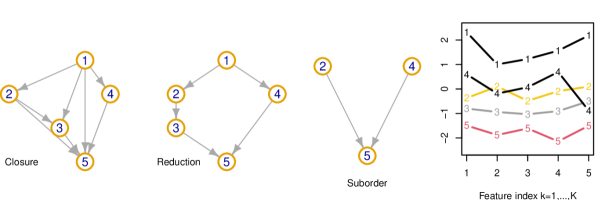
Figure 1: Partial order $H=\{\langle 1,2\rangle,\langle 1,3\rangle,\langle 1,4\rangle,\langle 1,5\rangle,\langle 2,3\rangle,\langle 2,5\rangle,\langle 3,5\rangle,\langle 4,5\rangle\},\ H\in{\mathcal{H}}_{[m]}$ on $[m]=(1,2,3,4,5)$ represented by its transitively closed directed acyclic graph (left) and transitive reduction (centre left). Suborder $H[O]$ for $O=\{2,4,5\}$ (centre right) and a possible $Z$-matrix representation of $H$ (right) with $y$-axis giving $Z$-value.

Let $\mathcal{P}_{[m]}$ be the set of all permutations of $[m]$. A linear extension of $H$ is any list $\ell=(\ell_{1},...\ell_{m}),\ \ell\in\mathcal{P}_{[m]}$ in which lesser entries come after greater entries, so $\ell_{j}\succ_{H}\ell_{k}$ is not allowed if $k<j$. For example, if $H$ is the partial order displayed in Fig 1 then $h$ has three linear extensions, $(1,2,3,4,5),(1,2,4,3,5)$ and $(1,4,2,3,5)$. Denote by

$$\mathcal{L}[H]=\{\ell\in\mathcal{P}_{[m]}:\langle\ell_{j},\ell_{k}\rangle\not\in H\ \mbox{for all}\ 1\leq k<j\leq m\}$$

the set of all linear extensions of $H\in{\mathcal{H}}_{[m]}$.

If we start with a social hierarchy $H\in{\mathcal{H}}_{[m]}$ over all actors then the hierarchy constraining any given subset $O\subseteq[m]$ of the actors is the suborder

$$H[O]=\{\langle j_{1},j_{2}\rangle\in H:\{j_{1},j_{2}\}\subseteq O\}$$ (2)

obtained by retaining only edges between vertices in $O$. If $H$ is a (transitively closed) partial order then so is $H[O]$. For example, in Fig 1, if $O=\{2,4,5\}$ then the suborder $H[O]$ is identified with the three-vertex DAG centre right.

2.2.2 Lists as randomly ordered queues

A single generic list $Y=(Y_{1},...,Y_{m})$ is modeled as a random linear extension of $H$. Let $C(H)=|\mathcal{L}[H]|$ be the number of linear extensions of partial order $H\in{\mathcal{H}}_{[m]}$. The “noise free” likelihood for $H$ is simply

$$p(Y|H)=C(H)^{-1}\mathbb{I}_{Y\in\mathcal{L}[H]}.$$ (3)

This observation model is motivated by thinking of each list as a realisation of a random queue process in which actors not ordered by $H$ randomly swap places. The equilibrium of this process is the uniform distribution on linear extensions of $H$ (Karzanov and Khachiyan, 1991), so if $Y$ is a snapshot of this queue at equilibrium then $Y\sim\mbox{Unif}(\mathcal{L}[H])$.

Computation of $C(H)$ is in #P (Brightwell and Winkler, 1991) so evaluating $p(Y|H)$ is prohibitive at large $m$. However, in our data $m$ is small enough to allow likelihood evaluation in reasonable time. For $j\in[m]$ let $\mathcal{L}_{j}[H]=\{\ell\in\mathcal{L}[H]:\ell_{1}=j\}$ be the set of linear extensions with $j$ first in the list and let $C_{j}(H)=|\mathcal{L}_{j}[H]|$. Partitioning on the first entry,

$$C(H)=\sum_{j=1}^{m}C_{j}(H),$$

which Knuth and Szwarcfiter (1974) compute using the suborder recursion in Supp C.1.

2.2.3 Queue jumping and suborders

We modify the likelihood in Eqn 3 in three ways: lists may be “noisy”; just a subset of actors are in any given list; lists are observed over time.

We allow for noise in the observation model by allowing individuals to “jump the queue”. A list $Y$ is formed by taking individuals from the top of a queue which continues to mix rapidly, constrained by the suborder on those remaining. Before the $j$’th actor is chosen, there are $m-j+1$ individuals (with labels $Y_{j:m}$) yet to be placed. With probability $p$ the next actor (ie $Y_{j}$) is chosen at random, ignoring any order constraints. Otherwise, $Y_{j}$ is chosen as the first actor in a random linear extension of the suborder $H[Y_{j:m}]$ for those remaining. The fraction of lists headed by $Y_{j}$ is $C_{Y_{j}}(H[Y_{j:m}])/C(H[Y_{j:m}])$. Working from the top down,

$$p_{(D)}(Y|H,p)=\mathbb{I}_{Y\in\mathcal{P}_{[m]}}\prod_{j=1}^{m}\left(\frac{p}{m-j+1}+(1-p)\frac{C_{Y_{j}}(H[Y_{j:m}])}{C(H[Y_{j:m}])}\right).$$ (4)

Noise allows any list to appear with non-zero probability. The noisy model reduces to $P(Y|H)$ in Eqn 3 when $p=0$ as the product of counts is telescoping.

We take $p\sim\mbox{Beta}(1,\delta)$ as our family of priors for the queue-jumping probability $p$. The prior hyperparameter $\delta\geq 1$ is fixed (for example, in Sec 6 we take $\delta=9$, so the prior probability for a queue-jumping event is about ten percent), expressing the belief that if order relations are present then they are respected.

In Eqn 4 individuals are promoted up the queue. We can also model random “demotion”. In this case the list is filled from the bottom up: with probability $p$ the next actor is chosen at random, ignoring any order constraints; otherwise, they are the last entry in a random linear extension of the suborder for the remaining individuals. The likelihood becomes

$$p_{(U)}(Y|H,p)=\mathbb{I}_{Y\in\mathcal{P}_{[m]}}\prod_{j=1}^{m}\left(\frac{p}{j}+(1-p)\frac{\tilde{C}_{Y_{j}}(H[Y_{1:j}])}{C(H[Y_{1:j}])}\right),$$ (5)

where $\tilde{C}_{Y_{j}}(H)$ is the number of linear extensions of $H$ which end with $Y_{j}$. Jiang et al. (2023) extend these models to allow random promotion and demotion in a single realised list. The likelihood is tractable, but evaluation is time consuming so we do not fit that model here.

2.2.4 Observation model for suborders

Suppose that, when $Y$ was realised, a subset $O=\{O_{1},...,O_{n}\},\ O\subseteq[m]$ of actors entered the queue. Since they were constrained by the suborder $H[O]$, the noise free observation model is $Y\sim\mbox{Unif}(\mathcal{L}[H[O]])$: the list is a random draw from the linear extensions of the suborder. For example, for $H$ in Fig 1, if $O=\{2,4,5\}$ then the linear extensions are $\mathcal{L}[H[O]]=\{(2,4,5),(4,2,5)\}$ and $Y$ is chosen at random from this set. The queue-jumping likelihoods $p_{(D)},p_{(U)}$ are obtained by replacing $H\to H[O],\ [m]\to O$ and $m\to n$ in Eqns 4 and 5.

2.2.5 Time series of lists

Finally, we restore time and give the full likelihood. At each time $t\in[B,E]$ the actors indexed in ${\mathcal{M}}_{t}$ were active and had relative status expressed by some partial order hierarchy $h^{(t)}\in{\mathcal{H}}_{{\mathcal{M}}_{t}}$. The sequence of partial orders from $B$ to $E$ is

$$h =(h^{(B)},h^{(B+1)},...,h^{(E)}),$$ (6)

where $$h\in{\mathcal{H}}^{(B,E)}$$ with

$${\mathcal{H}}^{(B,E)} ={\mathcal{H}}_{{\mathcal{M}}_{B}}\times{\mathcal{H}}_{{\mathcal{M}}_{B+1}}\times...\times{\mathcal{H}}_{{\mathcal{M}}_{E}}.$$ (7)

We refer to $h$ as a partial order time series (when it is a realisation) or a partial order process (once we have have defined the stochastic process that generates it).

For $i\in{\mathcal{I}}$, list $y_{i}$ was formed under constraints imposed by the suborder $h^{(\tau_{i})}[o_{i}]$ for $o_{i}\subseteq{\mathcal{M}}_{\tau_{i}}$ at the time $\tau_{i}$ that the list was made, that is, $y_{i}\in\mathcal{L}[h^{(\tau_{i})}[o_{i}]]$. The full likelihood is then

$$p(y|h,\tau,p)=\prod_{i=1}^{N}p(y_{i}|h^{(\tau_{i})}[o_{i}],p),$$ (8)

where $p(y_{i}|h^{(\tau_{i})}[o_{i}],p)$ is given by $p_{(D)}$ or $p_{(U)}$ in Eqns 4 or 5 (depending on our choice of model) with the replacements $Y\to y_{i}$, $m\to n_{i}$ and $H\to h^{(\tau_{i})}[o_{i}]$.

2.3 Latent variables and covariates in a prior for partial orders

We derive prior models for partial orders from $k$-dimensional random orders (Winkler, 1985). They are marginally consistent for suborders. This means the prior probability $\pi_{{\mathcal{H}}_{O}}(G)$ we define for a partial order $G\in{\mathcal{H}}_{O}$ on a subset $O\subset[m]$ is equal to its marginal probability computed from the prior $\pi_{{\mathcal{H}}_{[m]}}(H)$ for partial orders $H$ on the superset $[m]$. Dropping time,

$$\pi_{{\mathcal{H}}_{O}}(G)=\sum_{H\in{\mathcal{H}}_{[m]}}\pi_{{\mathcal{H}}_{[m]}}(H)\mathbb{I}_{G=H[O]}.$$ (9)

This relation is easily violated if one simply writes down a distribution $\pi_{{\mathcal{H}}_{[m]}}(H)$ for each $m\geq 1$. The uniform distributions $\mbox{Unif}({\mathcal{H}}_{[m]})$ are not marginally consistent. There are three partial orders for $m=2$ and nineteen for $m=3$, so if $H\sim\mbox{Unif}({\mathcal{H}}_{[3]})$ then we won’t have $H[(1,2)]\sim\mbox{Unif}({\mathcal{H}}_{[2]})$ as we can’t group the nineteen into three equal masses.

We would like to control the prior depth distribution as it is of interest in many applications. For example, if inference for depth is important then a prior which is non-informative with respect to depth will be useful. The uniform prior on partial orders is strongly informative with respect to depth, as it concentrates on partial orders of depth three as $m\to\infty$ (Kleitman and Rothschild, 1975). This effect is illustrated in Supp E.

2.3.1 Latent variable parameterisation

We use feature vectors, one for each actor, to determine actor-placing in the social hierarchy. These “status-features” do not correspond to any identifiable physical attributes. Following Winkler (1985), we associate with each actor $j\in{\mathcal{M}}_{t}$, at a time $t\in[b_{j},e_{j}]$, a $1\times K$ latent vector $Z^{(t)}_{j}\in\mathbb{R}^{K},\ Z^{(t)}_{j}=(Z^{(t)}_{j,1},...,Z^{(t)}_{j,K})$ of $K\geq 1$ status-features. Let $Z^{(t)}=(Z^{(t)}_{j})_{j\in{\mathcal{M}}_{t}}$ be an $m_{t}\times K$ status matrix, with one row for each actor active at time $t$ and one column for each status feature $1,...,K$.

The partial-order $h^{(t)}$ at time $t$ is a function of $Z^{(t)}$. At time $t$ actor $j\in{\mathcal{M}}_{t}$ is above actor $j^{\prime}\in{\mathcal{M}}_{t}$ if all status variables of $j$ are greater than those of $j^{\prime}$, that is, $h^{(t)}=h(Z^{(t)})$ with

$$h(Z^{(t)})=\{\langle i,j\rangle\in{\mathcal{M}}_{t}\times{\mathcal{M}}_{t}:Z^{(t)}_{i,k}>Z^{(t)}_{j,k}\ \mbox{for all $k=1,...,K$}\}.$$ (10)

The setup is illustrated in Fig 1 at right. The rows of $Z^{(t)}$ are “paths” in the space $[K]\times\mathbb{R}$: the relation $\langle j,j^{\prime}\rangle\in h^{(t)}$ holds when the path $(k,Z^{(t)}_{j,k})_{k=1}^{K}$ lies above the path through $(k,Z^{(t)}_{j^{\prime},k})_{k=1}^{K}$; if the paths cross then the actors are unordered. In Fig 1, the $Z$-path for actor 4 intersects the paths for 2 and 3. The other paths do not intersect. This is a latent feature representation of the partial order at left. In Winkler (1985) the columns of $Z^{(t)}$ are independent and paths are likely to cross. By contrast, the priors we give in Sec 2.3.3 correlate columns and give us some control over the prior depth distribution.

In our parameterisation we take a fixed value of $K$. Using results from (Hiraguchi, 1951; Bogart, 1973), it may be shown that if $K\geq\lfloor m_{t}/2\rfloor$ then any partial order $h^{(t)}\in{\mathcal{M}}_{t}$ can be represented by some $m_{t}\times K$ matrix $Z^{(t)}$. This is discussed in a modelling context in Muir Watt (2015) and proven in Sec 3.2 below. Since $h^{(t)},\ t\in[B,E]$ has at most $D$ vertices (see Eqn 1), a model with $K\geq\lfloor D/2\rfloor$ can represent any partial order process $h\in{\mathcal{H}}^{(B,E)}$.

2.3.2 Covariate effects for partial orders

.

In Sec 2.1 we introduced an actor-specific covariate informing status relations among actors. In the following $s_{t,j}\in\{1,2,\ldots,S\}$ is a single categorical or ordinal variable with levels from 1 to $S$. More general covariates are easily accommodated. Let $\beta\in\mathbb{R}^{S}$ be the vector of level effects. We split the status vector $Z^{(t)}_{j}$ of actor $j\in{\mathcal{M}}_{t}$ into an additive effect $\beta_{s_{t,j}}$ due to $s_{t,j}$ and an “authority-vector” $U^{(t)}_{j}\in\mathbb{R}^{K}$, which captures all aspects of status which are not attributable to the covariate. Our additive model is, for $j\in{\mathcal{M}}_{t}$ and $t\in[B,E]$,

$$Z^{(t)}_{j}=U^{(t)}_{j}+1_{K}\beta_{s_{t,j}}$$ (11)

where $1_{K}$ is a row vector of $K$ ones. Higher $\beta_{s_{t,j}}$-values lift all components of $U^{(t)}_{j}$ by a constant, raising the status features in $Z^{(t)}_{j}$. This moves the path $(k,Z^{(t)}_{j,k})_{k=1}^{K}$ above other paths and gives a higher position for actor $j$ in the partial order $h^{(t)}$.

In our application the covariate is ordinal with a greater effect expected for lower values of $s$ so we will be interested in testing for $\beta_{1}>\beta_{2}>...>\beta_{S}$. Let $\mathcal{B}_{0}=\mathbb{R}^{S}$ and

$$\mathcal{B}_{S}=\{\beta\in\mathcal{B}_{0}:\beta_{1}>\beta_{2}>...>\beta_{S}\}.$$ (12)

We carry out analyses under models with $\beta\in\mathcal{B}_{0}$ (to check our prior expectation that $\beta\in\mathcal{B}_{S}$) and then again with $\beta\in\mathcal{B}_{S}$ (for best estimation with a well supported subjective prior).

Let $Z=(Z^{(t)})_{t=B}^{E}$ and $U=(U^{(t)})_{t=B}^{E}$ and write $Z=Z(U,\beta;s)$ for the function defined in Eqn 11. The parameters $U$ and $\beta$ replace $h$ in the likelihood via $h=h(Z(U,\beta;s))$.

2.3.3 Prior probability distributions

We model the $K$-dimensional authority-process $U_{j}=(U^{(t)}_{j})_{t=b_{j}}^{e_{j}}$ for actor $j\in{\mathcal{M}}$ as a vector autoregression of order one with times-series correlation parameter $\theta$ and covariance $\Sigma^{(\rho)}$. In our model latent authority-features are correlated from one time step to another with a drift towards zero.

Our prior for the process $U_{j}$ is independent over $j\in{\mathcal{M}}$ with correlation parameters $0\leq\theta\leq 1$ and $0\leq\rho\leq 1$. Let $\Sigma^{(\rho)}$ be a $K\times K$ covariance matrix with diagonal elements $\Sigma^{(\rho)}_{k,k}=1$ and off diagonal $\Sigma^{(\rho)}_{k,k^{\prime}}=\rho$ for $k,k^{\prime}\in[K]$. Let $0_{K}$ be a vector of $K$ zeros. For $j\in{\mathcal{M}}$ let

$$U^{(b_{j})}_{j} \sim N\left(0_{K},\frac{\Sigma^{(\rho)}}{(1-\theta)^{2}}\right)$$

and for $$\epsilon^{(t)}_{j} t\in[b_{j}+1,e_{j}] j$$ iid for and each ,

$$U^{(t)}_{j} =\theta U^{(t-1)}_{j}+\epsilon^{(t)}_{j}\,,\hskip 8.5359pt\epsilon^{(t)}_{j}\sim N(0,\Sigma^{(\rho)})\,.$$ (13)

Write $U_{j}\sim\mbox{VAR}^{(b_{j},e_{j})}_{K,\rho,\theta}(1),\ j\in{\mathcal{M}}$ for the vector auto-regression with density

$$\pi(U_{j}|\rho,\theta)=N\left(U^{(b_{j})}_{j};0_{K},\frac{\Sigma^{(\rho)}}{(1-\theta^{2})}\right)\prod_{t=b_{j}+1}^{e_{j}}N\left(U^{(t)}_{j};\theta U^{(t-1)}_{j},\Sigma^{(\rho)}\right)\,.$$ (14)

The parameter $\rho$ controls the depth of realised partial orders. When $\rho\simeq 1$ paths $(k,U^{(t)}_{j,k})_{k=1}^{K}$ are relatively flat (like path 3 in Fig 1) as path-entries are strongly correlated. They are less likely to intersect so there are more order relations and $d(h^{(t)})$ is larger. When $\rho$ is close to zero the paths $U^{(t)}_{j}$ are more jagged (like path 4) so there are fewer order relations and $d(h^{(t)})$ is smaller. We take as our prior $\rho\sim\mbox{Beta}(1,\gamma)$ with $\gamma$ fixed. Prior simulation (Supp E, Fig 17, left) showed that taking $K=\lfloor D/2\rfloor$ and $\gamma=1/6$ gave a prior on partial orders which is acceptably uniform on depth. Our prior on $\theta$ is uniform, $\theta\sim\mbox{Unif}(0,1)$.

Our prior density for $\beta$ is $\pi_{\beta}(\beta)=N(\beta;0,I_{S})$. The variation between levels of a covariate equals the variation in authority over one time step: $\beta_{j}-\beta_{j^{\prime}}$ has the same variance as the components of $U^{t}_{j}-U^{(t-1)}_{j}$ in Eqn 13. We set $\Sigma^{(\rho)}_{k,k}=1$ as we can scale $\rho$ and the variance of $\beta$ to get the same distribution for $h$. It is necessary to take proper priors for $U$ and $\beta$. We discuss these priors further in Sec 4.2 in relation to identifiability.

2.4 Prior summary and Posterior distribution

We now summarise our generative model for the data. The model is depicted in Fig 2.

Figure 2: The generative model for lists is a HMM with latent process $U$ and emitted data $y$. Here $\rho$ and $\theta$ are hyperparameters in the $U$-prior, and $\beta$ and $U$ determine partial orders $h^{(t)}=h(Z(U^{(t)},\beta,s)$ (double lines and implication $\Rightarrow$). The distribution of lists $y_{i}$ observed at time $t=\tau_{i}$ is given by $h^{(t)}$ and $p$.

The data are the lists $y$. We condition on knowledge of the uncertainty ranges $\tau^{\pm}$, the covariate data $s$, the actor activities ${\mathcal{M}}_{t},\ t\in[B,E]$ and the prior hyper-parameters $\gamma,\delta>0$ and $K\geq 1$. The generative model is,

$$\rho \sim\mbox{Beta}(1,\gamma), \gamma=1/6$$ with unless stated,

$$\theta \sim\mbox{Unif}(0,1),$$

$$U_{j} \sim\mbox{VAR}^{(b_{j},e_{j})}_{K,\rho,\theta}(1), K=\lfloor D/2\rfloor U$$ with unless stated, and in Eqn 13,

$$\quad\mbox{iid for}\ j\in{\mathcal{M}},\ \mbox{with $U^{(t)}_{j}$ defined for $t:j\in{\mathcal{M}}_{t}$}$$

$$\beta \sim N(0,I_{S}), \quad\mbox{either $\beta\in\mathcal{B}_{0}$ or constrained $\beta\in\mathcal{B}_{S}$ per Eqn~{}\ref{eq:beta-constrained-space}}.$$

These collectively determine the partial-order prior via

$$Z =Z(U,\beta;s), Z=(Z^{(t)})_{t=B}^{E}$$ from Eqn 11, giving , and

$$h =h(Z(U,\beta;s)), \quad\mbox{from Eqn~{}\ref{eq:z-to-h-mapping}, giving $h=(h^{(t)})_{t=B}^{E}$};$$ (15)

Priors for the remaining observation model parameters are

$$\tau_{i} \sim U\{\tau^{-}_{i},\tau^{+}_{i}\}, \quad\mbox{independently for}\ i=1,...,N,\ \mbox{and}$$

$$p \sim\mbox{Beta}(1,\delta); \delta\geq 1 \delta=9$$ with and by default.

Finally the data are realised

$$y_{i} \sim p(\cdot|h^{(\tau_{i})}[o_{i}],p), \quad\mbox{independently for $i\in{\mathcal{I}}$},$$ (16)

using the distribution for $y_{i}$ given in Eqn 4 or 5. The joint posterior distribution is

$$\pi(\rho,\theta,U,\beta,\tau,p|y)\propto\pi(\rho,\theta,\beta,\tau,p)\pi(U|\rho,\theta)p(y|U,\beta,\tau,p)\,,$$ (17)

where

$$\pi(U|\rho,\theta) =\prod_{j\in{\mathcal{M}}}\pi(U_{j}|\rho,\theta)$$

$$p(y|U,\beta,\tau,p) =\prod_{i=1}^{N}p(y_{i}|h^{(\tau_{i})}[o_{i}],p),$$

with $\pi(U_{j}|\rho,\theta)$ given in Eqn 14 and $h$ depending on $U,\beta$ through Eqn 15. The model without covariates or time is given in Nicholls and Muir Watt (2011) and set out in Supp M.

3 Properties of priors

Our partial order prior is marginally consistent and expresses any partial order time series in ${\mathcal{H}}^{(B,E)}$. Supp E explores the prior using simulation.

3.1 Marginal consistency

Winkler (1985) shows marginal consistency when the columns of $Z^{(t)}$ are independent. We extend this to a stochastic process with columns correlated within and across time. We take $\beta=0_{S}$, so no covariates, as we cannot expect marginal consistency when we have covariate information which explicitly breaks it. When $\beta=0_{S}$ we have $Z^{(t)}_{j}=U^{(t)}_{j}=Z(U^{(t)}_{j},0_{S};s)$ for each $t\in[B,E]$ and each $j\in{\mathcal{M}}_{t}$. Let

$$\pi_{{\mathcal{H}}^{(B,E)}}(h|\rho,\theta,\beta=0_{S})=\int\mathbb{I}_{h=h(Z(U,0_{S};s))}\pi(U|\rho,\theta)\,dU$$

give the marginal distribution of $h$ given $\rho,\theta$ and $\beta=0_{S}$. The marginal distribution of $h$ is

$$\pi_{{\mathcal{H}}^{(B,E)}}(h|\beta=0_{S})=\int_{[0,1]^{2}}\pi_{{\mathcal{H}}^{(B,E)}}(h|\rho,\theta,\beta=0_{S})\pi(\rho,\theta)\,d\rho d\theta.$$ (18)

We can remove $j\in{\mathcal{M}}$ “from the beginning” or from the realised partial order “at the end” and get the same random partial order. In the former, the random partial order at time $t$ is $h(Z^{(t)}_{-j})$ where $Z^{(t)}_{-j}$ is an $m_{t}-1\times K$ matrix with one independent row $Z^{(t)}_{j^{\prime}}$ for each $j^{\prime}\in{\mathcal{M}}_{t}\setminus\{j\}$. Let $h(Z_{-j})=(h(Z^{(t)}_{-j}))_{t=B}^{E}$ be a time-series of partial orders realised in this way. In the latter, we take a suborder at the end. Let ${\mathcal{M}}^{-j}_{t}={\mathcal{M}}_{t}\setminus\{j\}$ and let $h^{(t)}_{-j}=h(Z^{(t)})[{\mathcal{M}}^{-j}_{t}]$ be the suborder at time $t$ when we remove $j$ from the order realised on the full $Z$-matrix. Let $h_{-j}=(h^{(t)}_{-j})_{t=B}^{E}$ give the time-series. Let

$${\mathcal{H}}^{(B,E)}_{-j}={\mathcal{H}}_{{\mathcal{M}}^{-j}_{B}}\times{\mathcal{H}}_{{\mathcal{M}}^{-j}_{B+1}}\times...\times{\mathcal{H}}_{{\mathcal{M}}^{-j}_{E}},$$

so that $h(Z_{-j})$ and $h_{-j}$ are both in ${\mathcal{H}}^{(B,E)}_{-j}$.

Proposition 1.

Let $g\in{\mathcal{H}}^{(B,E)}_{-j}$ be given. The prior in Eqn 18 is marginally consistent,

$$\pi_{{\mathcal{H}}^{(B,E)}_{-j}}(g|\beta=0_{S})=\sum_{h\in{\mathcal{H}}^{(B,E)}}\mathbb{I}_{g=h_{-j}}\pi_{{\mathcal{H}}^{(B,E)}}(h|\beta=0_{S}).$$

for each $j\in{\mathcal{M}}$. [See Supp B.1 for proof]

Proposition 1 establishes marginal consistency for removing one element of ${\mathcal{M}}$. Consistency for more general marginals follows by removing multiple elements one at a time.

We removed covariates in the analysis above. In some settings, covariate levels $s_{t,j},\ j\in{\mathcal{M}}_{t}$ characterise relations between actors active at time $t$ and would change if we add or remove a actor. However, if covariate levels $s_{t,j}$ are intrinsic then they don’t change when we add and remove actors. In that case $Z^{(t)}_{j_{1}}=U^{(t)}_{j_{1}}+1_{K}\beta_{s_{t,j_{1}}}$ doesn’t change when we add or remove actor $j_{2}$ and so relations between $j_{1}$ and a third actor $j_{3}$ don’t change. It is then straightforward to show that $\pi_{{\mathcal{H}}^{(B,E)}}(h|\beta)$ is consistent for every $\beta$ and so $\pi_{{\mathcal{H}}^{(B,E)}}(h)$ is also.

3.2 Universal representation

We claimed in Sec 2.3.1 that, if $K\geq\lfloor D/2\rfloor$ with $D$ defined in Eqn 1 then any partial order $h^{(t)}\in{\mathcal{H}}_{{\mathcal{M}}_{t}}$ can be represented by some $m_{t}\times K$ matrix $Z^{(t)}$. We restore $\beta\in\mathcal{B}_{0}$ or $\mathcal{B}_{S}$ and covariate effects. Let

$$\pi_{{\mathcal{H}}^{(B,E)}}(h)=\int_{\mathbb{R}^{S}}\pi_{{\mathcal{H}}^{(B,E)}}(h|\beta)\pi(\beta)\,d\beta$$ (19)

be the full marginal prior with variable $\beta$, extended from Eqn 18.

Proposition 2.

Suppose $\min_{t\in[B,E]}m_{t}\geq 4$. The probability $\pi_{{\mathcal{H}}^{(B,E)}}(h)$ in Eqn 19, given by the generative model Eqn 15 with $K\geq\lfloor D/2\rfloor$, assigns a positive probability mass $\pi_{{\mathcal{H}}^{(B,E)}}(h)>0$ to every timeseries $h\in{\mathcal{H}}^{(B,E)}$. [See Supp B.2 for proof.]

4 Computational methods

4.1 Markov Chain Monte Carlo

We implemented an MCMC algorithm targeting $\pi(\rho,\theta,U,\beta,\tau,p|y)$ in Eqn 17. Each update is a simple Metropolis-Hastings MCMC step. The updates are summarised in Supp F. We checked the implementation of the likelihood by simulating synthetic data and checking list proportions matched their probability in the likelihood. We also recover the true parameters of synthetic data (see Fig L.1). We run the MCMC producing $L$ samples (after burn-in and thinning) $\rho^{(l)},\theta^{(l)}$, $U^{(t,l)}=(U^{(t,l)}_{j})_{j\in{\mathcal{M}}_{t}}$, $\beta^{(l)},\tau^{(l)}$ and $p^{(l)}$ for $l=1,...,L$. This determines samples for $Z^{(t,l)}=(Z^{(t,l)}_{j})_{j\in{\mathcal{M}}_{t}}$, with

$$Z^{(t,l)}_{j}=U^{(t,l)}_{j}+1_{K}\beta^{(l)}_{s_{t,j}}$$

and similarly $h^{(t,l)}=h(Z^{(t,l)})$, for $t=B,...,E$ and $l=1,...,L$.

4.2 Posterior summaries

Besides plotting marginals for individual parameters $\rho,\theta,p$ and $\beta$, we report selected summary statistics computed on the MCMC output. These are the consensus partial order (which displays relations with posterior support greater than one half, see Supp G) and the Bayes factor for the first $S^{\prime}$ of the $S$ covariate effects to be ordered, $\mathcal{B}_{S^{\prime}}=\{\beta\in\mathcal{B}_{0}:\beta_{1}>\beta_{2}>...>\beta_{S^{\prime}}\}$. This Bayes factor is the ratio of marginal likelihoods

$$B_{S^{\prime},0}=\frac{p(y|\beta\in\mathcal{B}_{S^{\prime}})}{p(y|\beta\in\mathcal{B}_{0})}.$$

Formulae for estimating these quantities are given in Supp G.

4.2.1 Non-identifiability of $U$ and $\beta$

We are interested in separating the relative authority $U^{(t)}_{j}$ of a actor from the status $Z^{(t)}_{j}$. There are two sources of non-identifiability. The latent variables $U$ have a label swapping symmetry: the posterior is invariant under permutation of the columns of the $M_{t}\times K$ matrix $U^{(t)}$ if the same permutation is applied at each $t\in[B,E]$. One simple summary which is invariant under column permutation is the row-average,

$$\bar{U}^{(t,l)}_{j}=\frac{1}{K}\sum_{k=1}^{K}U^{(t,l)}_{j,k},$$

measuring the authority of actor $j$ at time $t$. The estimated posterior authority is

$$\bar{U}^{(t)}_{j}=\frac{1}{L}\sum_{l=1}^{L}\bar{U}^{(t,l)}_{j}.$$ (20)

We plot $\bar{U}^{(t)}_{j}$ as a function of $t$ for each $j$. The average status $\bar{Z}^{(t)}_{j}$ is defined similarly.

The second source of non-identifiability is shift invariance of $h^{(t)}$ under

$$U^{(t)}_{j} \to U^{(t)}_{j}+1_{K}u^{(t)},\ t\in[B,E],\ j\in{\mathcal{M}}_{t},$$ (21)

$$\beta_{r} \to\beta_{r}+c,\ r\in[S],$$ (22)

where $u^{(t)}\in\mathbb{R}$ is a common shift applied to each actor, which may vary over $t$, and $c\in\mathbb{R}$ is common shift applied to all effects. The proper $U$ and $\beta$ priors shrink these shifts towards zero. We project these degrees of freedom out by subtracting the averages, $\bar{U}^{(t)}_{j}\to\bar{U}^{(t)}_{j}-{\mathcal{M}}_{t}^{-1}\sum_{j}\bar{U}^{(t)}_{j}$ and $\beta_{r}\to\beta_{r}-S^{-1}\sum_{r^{\prime}}\beta_{r^{\prime}}$, before computing the summary statistics and plotting. A similar issue arises in the Plackett-Luce time-series model in Supp K.1.

5 Introduction to the data

The model set out in Sec 2.4 was motivated by a dataset in which lists $y_{i},\ i\in{\mathcal{I}}$ record the names of individuals witnessing legal documents from the late eleventh and twelfth century. It is clear that names were written down in an order that respects some unknown measure of social standing, though many factors have have contributed to individual status. Our model, in which lists gathered in year $t$ respect an incomplete social hierarchy $h^{(t)}$ which is known and respected by all but subject to occasional change, directly represents the evolving underlying social hierarchy of the day. However, there was no “queue”: the witness lists were written down by a royal scribe with (we assume) perfect knowledge of the universally agreed hierarchy, so the queue model is an idealisation.

5.1 Context

Each witness list in the data is an ordered list of names of individual witnesses taken from a single legal document or “act” (collectively “acta”). A typical example (with List id 2364) is given in Supp A.2. This study draws on an accumulated dataset, accessed through the database made for ‘The Charters of William II and Henry I’ project by the late Professor Richard Sharpe and Dr Nicholas Karn (Sharpe et al., 2014). Some historical background on these data is given in Supp A.1.

We have 1610 witness lists dated between 1066 CE and about 1166 CE involving 1760 individuals. A witness list is a “snapshot” created at a single event on a single day. We assume distinct lists are generated independently (for example, we see no evidence for a pair of Acta created at the same time with identical lists). Acta are witnessed in order of social rank from the king or queen, archbishop, bishops (as a group), earls (as a group, may precede bishops) and so on down through society. Historians ask if the order in which bishops appear within the their sub-list reflects their evolving personal authority. We represent and infer these relations.

We take time as discrete by year as the data gives dates rounded to the year. Further coarsening would mask recoverable structural change. Outside the range $[B=1080,E=1155]$ CE the lists are sparse so we focus on this interval, covering the reigns of William II, Henry I and Stephen and $T=E-B+1=76$ years. The period is long enough for us to witness changes in the status of individual bishops, but short enough for there to be some hope of temporal homogeneity in the social conventions mapping status to witness list.

5.2 Witness list data

Data processing is set out in Supp A.2 and A.5.

Bishops from thirty one dioceses appear in the data (including one, Tusculum, from Italy). They are listed in Supp A.3 and can be seen at the left side of Fig 3.

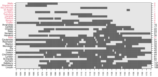
Figure 3: The left axis gives dioceses colored black (included) or red (excluded). The right axis gives the number of lists in which each diocese is represented. The $x$-axis gives the date in years. In any given year a diocese may be occupied with a bishop in-post (dark cell) or unoccupied (light).

We selected twenty Anglo-Norman dioceses (fourteen from England and six from Normandy) in our analysis and dropped eleven, appearing in a relatively small number of lists.

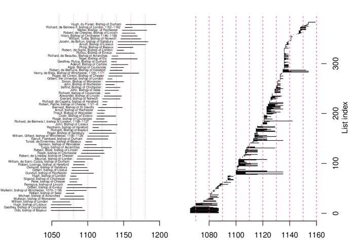
Figure 14: Bishop (left) and list (right) date intervals. Each horizontal bar above left spans the interval $[b_{j},e_{j}]$ over which the indicated bishop $j\in{\mathcal{M}}$ held their appointment. Each bar above right spans the uncertainty interval $[\tau^{-}_{i},\tau^{+}_{i}]$ for list $i\in{\mathcal{I}}$.

The dates of 213 lists are uncertain. Upper and lower date bounds are available for these (the mean interval length is 4 years, and 90% span less than 10 years). As in Sec 2.1, $\tau^{\pm}_{i}=(\tau^{-}_{i},\tau^{+}_{i})$ gives the available year bounds for the $i$’th list. Date intervals $[\tau^{-}_{i},\tau^{+}_{i}]$ are plotted in Supp A in Fig 14 at right. Fig 4 plots lists and their lengths againt their dates (using the midpoint of $[\tau^{-}_{i},\tau^{+}_{i}],\ i\in{\mathcal{I}}$).

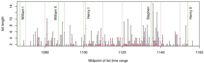
Figure 4: List lengths and dates. Green lines are coronation dates of indicated Kings, red dashed lines at decades, black bar height is longest list at that date, one (jittered) red dot for each list plotted at (date,length).

We include a list if at least half its interval falls within the 76-year interval $[B,E]$; most of the lists in our analysis fall entirely within it.

Many of the lists contain less than two bishops. We extract $N=371$ lists, dated between $B=1080$ and $T=1155$, and containing two or more bishops. We refer to this as the “full data”. Each of the $M=59$ bishops in at least two lists is assigned a numerical index from $1$ to $M$ in Fig 24 in Supp H.2. This data selection is detailed in Supp A.5.

Our information about a bishop’s status is limited by the number of lists in which a bishop appears. However, longer lists are more informative, as they inform relations between many pairs of bishops. Fig 5 shows the distribution of the number of lists a bishop appears in and the distribution of list lengths.

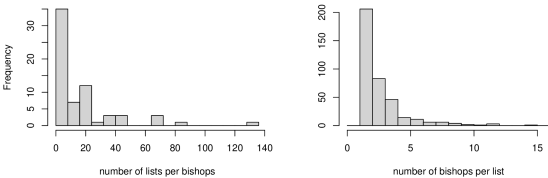
Figure 5: Frequency of lists per bishop, a histogram of the counts $\sum_{i\in{\mathcal{I}}}\mathbb{I}_{j\in o_{i}}$, is plotted at left. Distribution of list lengths, a histogram of the counts $n_{i}=|o_{i}|$, is plotted at right.

Most bishops appear in a small number of lists and most lists are relatively short. However, lists “link together”. If two bishops $j_{1},j_{2}$ do not appear in any list together, but $j_{1}$ comes before $j_{3}$ in some list and $j_{3}$ before $j_{2}$ in another, then this is evidence for $j_{1}$ having higher status than $j_{2}$. This evidence accumulates over lists.

5.3 Seniority covariates

For $j\in{\mathcal{M}}$ we have (FEA, 2022) dates of appointment $b_{j}<E$ and death $e_{j}>B$ for each bishop. The distribution of these intervals can be seen in Supp A in Fig 14 at left. The intervals match the list date-ranges $(\tau^{-}_{i},\tau^{+}_{i})$ so that no bishop appears in a list when not in post. At any given time some dioceses may be empty so the number $m_{t}=|{\mathcal{M}}_{t}|$ of “active” bishops in post may vary from year $t$ to year $t+1$. Fig 3 shows the presence and absence of bishops by diocese.

A bishop’s “seniority” may have contributed to their overall status, so it is a covariate in our model for the hierarchy of bishops. The first canon of the Council of London in 1075 concerns precedence: “…each man shall sit according to his date of ordination, except for those who have more honourable seats by ancient custom or by the privileges of their churches” (Clover and Gibson, 1979); in year $t$ the longest serving bishop has seniority-rank one, and the last appointed bishop has rank at most $m_{t}$. Denote by $s_{t,j}\in\{1,...,m_{t}\}$ the seniority-rank of bishop $j\in{\mathcal{M}}$ in year $t\in\{b_{j},b_{j}+1,...,e_{j}\}$. We define seniority-rank as

$$s_{t,j}=\sum_{k\in{\mathcal{M}}_{t}}\mathbb{I}_{b_{j}\geq b_{k}}.$$ (23)

Bishops have equal seniority if there are ties in the start dates $b_{j},\ j\in{\mathcal{M}}$. The greatest seniority observed, $S=\max_{t,j}s_{t,j}$, is less than or equal $D$, the most bishops active.

Fig 6 shows seniority-rank traces for each bishop from their first to last year in post. Bishops progress in rank by about one place every one or two years, more rapidly at first, as there are more bishops ahead of them. Our estimates of the effect $\beta_{r}$ of possessing seniority-rank $r\in\{1,...,S\}$ depends for precision on a bishop with seniority $r$ appearing in a reasonable number of lists, so we plot the occurrence frequency $f_{r}=\sum_{i\in{\mathcal{I}}}\sum_{j\in o_{i}}\mathbb{I}_{s_{\tau_{i},j}=r}$ against $r$ to see which levels of the covariate are well represented in the data. High $r$-values (bishops with the least seniority) appear rarely, so their $\beta_{r}$-posterior distributions resemble their priors.

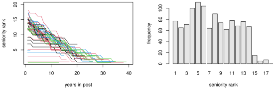
Figure 6: Seniority rank covariate $s$ defined in Eqn 23. Rank $s_{t,j}$ is plotted against “years in post”, $t-b_{j}$, for each bishop $j\in{\mathcal{M}}$ (Left). The frequency of seniority-rank $r$ in lists is plotted against $r$ from 1 to $S$ (Right).

Some dioceses were more peaceful and wealthy than others, so we considered taking diocese label as a second covariate for status. However, diocese would be colinear with bishop label (ie, $U_{j}^{(t)}$), as each bishop only occupies one diocese in the period of study. An effect due to diocese would not be identifiable with the effects due to the bishops in that diocese.

6 Results

6.1 Fitted models

Prior distributions are summarised in Sec 2.4. Unless otherwise stated we present results for the likelihood $p_{(U)}$ in Eqn 5. Experiments showed slightly lower estimated noise probabilities $p$ for $p_{(U)}$ than $p_{(D)}$ (see Eqn 4 and Fig 21, where the effect is slight). In analyses of some shorter time periods (not reported) the difference in $p$-posteriors was larger. We interpreted this lower noise in $p_{(U)}$ to mean the $p_{(U)}$ model is a better fit, but there is little difference in the distribution of quantities of interest, such as $\beta,U$ and $h$.

The greatest number of active bishops $D=19$ so we take $K=9$ (per the discussion at the end of Sec 2.3.1) for the dimension of the latent status feature vectors $Z^{(t)}_{j},\ j\in{\mathcal{M}},t\in[B,E]$ in our main analyses in Secs 6.2 and 6.3. We check robustness using $K=18$ in a second analysis in Sec H.3 of Supp H. The $\beta$-dimension is $S=18$ reflecting a tie at seniority-rank 18 in the year (1133) with the largest maximum seniority-rank.

6.2 Analysis with unconstrained seniority effects

We begin by presenting our results for the full data set defined in Sec 5.2. We first check that we see declining seniority effect at lower seniority, so we do not constrain the seniority effects to be ordered and take $\beta\in\mathcal{B}_{0}$.

Traces in Fig 22 in Supp H.1 for MCMC targeting the posterior in Sec 2.4 show convergence. Marginal posterior densities from two independent runs are shown in Fig 7. The correlation $\rho$ of features in $U^{(t)}_{j},\ j\in{\mathcal{M}}$ at each fixed time $t\in[b_{j},e_{j}]$ is close to one, supporting relatively deeper partial orders. The time-series correlation parameter $\theta$ is close to one, indicating strong serial correlation between $U^{(t)}_{j}$ and $U^{(t+1)}_{j}$, and therefore also $h^{(t)}$ and $h^{(t+1)}$. Finally, the error probability $p$, which controls the extent to which lists $y_{i}$ may depart from the linear extensions $\mathcal{L}[h^{(\tau_{i})}]$, is small, as we would expect if the partial order model captures the variation in lists. The prior for $p$ has $\delta=9$, favoring small $p$. We checked robustness to this choice: Fig 7 shows the prior and the posterior density when $\delta=1$ (uniform, estimated by importance sampling reweighting); this agrees with the $\delta=9$ posterior.

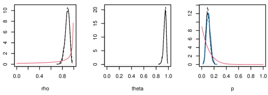
Figure 7: Posterior parameter densities for $\rho,\theta$ and $p$ from the unconstrained seniority effects analysis in Sec 6.2. Two independent MCMC runs are shown (solid and dashed). The red curve in the $\rho$ and $p$ graphs is their prior. The prior for $\theta$ is uniform. The blue curve in the $p$-density is the posterior density for a uniform prior on $p$.

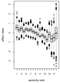
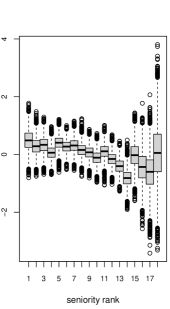
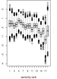
Figure 8: (Left) Marginal posterior distributions of seniority effect parameters from the unconstrained seniority effects analysis in Sec 6.2 with likelihood $p_{(U)}$ in Eqn 5. (Centre) As left with likelihood $p_{(D)}$ in Eqn 4. (Right) Corresponding distributions estimated using the Plackett-Luce time-series model in Supp K.1.

In Fig 8 (Left) we plot marginal posterior $\beta$ distributions in the posterior with likelihood $p_{(U)}$ (noise is random downward displacement). There is a clear downward trend with increasing seniority-rank value (ie, lower seniority). When the rank is large (15-18) we have few instances of bishops with that rank (see Fig 6), and distributions trend back to the prior.

Under observation model $p_{(U)}$, the effect $\beta_{11}$ is “out of order”. This is because several bishops who spent three or more years at seniority-rank 11 (William Giffard, bishop of Winchester, Richard de Belmeis I, bishop of London and Henry de Blois, Bishop of Winchester) were connected with royalty and started with high status among bishops. The likelihood $p_{(U)}$ has difficulty accommodating this event as it only models downward displacements so this event becomes evidence for something special about seniority-rank 11. In Fig 8 (Centre) we plot same quantities estimated using the $p_{(D)}$ likelihood (noise is upward displacement). The events at seniority-rank 11 can be modelled as a small number of upward “noise” displacement events using $p_{(D)}$. The centre graph correspondingly shows a more regular trend with seniority. In fact this event isn’t noise; these bishops $j\in{\mathcal{M}}$ simply had high values of $U^{(b_{j})}_{j}$ from the start. This is best modeled by imposing the seniority-effect order constraint $\beta\in\mathcal{B}_{S}$ as we do in Sec 6.3 below. We had good reason to do that anyway, as noted in Sec 2.3.2.

When we estimate the Bayes factor $B_{S^{\prime},0}$ in Eqn 30 up to $S^{\prime}=9$ we find $\hat{B}_{6,0}=3.0(0.7)$, $\hat{B}_{7,0}=6(2)$, $\hat{B}_{8,0}=19(13)$ and $\hat{B}_{9,0}=84(83)$ with standard errors from iid Bernoulli sampling in parenthesis (rare events in the MCMC, so effectively iid). The last of these is based on a single MCMC sample with $\beta\in\mathcal{B}_{9}$. However, given the improbability of these states in the prior ($1/9!$), seeing any samples at all with this pattern is evidence for increasing seniority effects with increasing seniority. We see in this analysis the structures we anticipated.

6.3 Analysis with constrained seniority effects

The assumption of decreasing seniority effect with higher lower seniority is supported on historical and statistical grounds. Since it is likely to hold, we now conduct an analysis under the constraint $\beta\in\mathcal{B}_{S}$. The $\rho,\theta$ and $p$ posterior densities are essentially unchanged from Fig 7 so we do not report them. Marginal posterior distributions for the unknown list dates $\tau_{i},\ i\in{\mathcal{I}}$ are given in Fig 26 in Supp H.2. We learn little there as the prior constraints $\tau_{i}\in[\tau^{-}_{i},\tau^{+}_{i}]$ are already quite tight. However, the residual uncertainty is integrated into other estimates.

In Fig 9 we plot the partial orders $h^{(t,l)},t=1136-1138$ from one MCMC sample state (the final sample) selected from the sequence of partial order time-series $(h^{(t,l)})_{t\in[B,E]},\ l=1,...,L$ output by the MCMC.

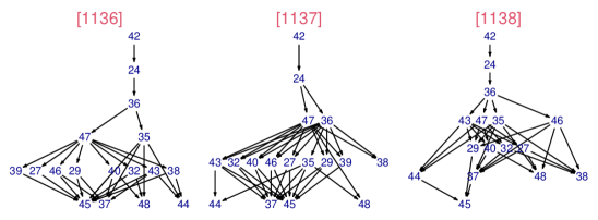
Figure 9: A small part of one MCMC-sampled state, from the constrained seniority effects analysis in Sec 6.3, showing the fitted partial order time-series between 1136 and 1138 (it runs from 1080 to 1155). Vertex numbers correspond to bishops names in Fig 24 in Supp H.2.

We select these three years after Stephen came to the throne in 1135 as illustrative. The number and length of lists in this period is relatively large (see Fig 4). In Fig 10

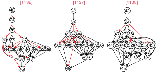
Figure 10: Consensus partial orders for the years 1136-1138 (a selection from 1080-1155) under the constrained-effects model of Sec 6.3. These are transitive reductions. Closures are given in Fig 23 in Supp H.2. Edges have posterior support at least $\xi=0.5$. Red edges have support above $0.9$. Vertex numbering as Fig 9.

we plot posterior consensus partial orders $\bar{h}^{(t)}$ (see Sec 4.2) estimated at the same years. We plot transitive reductions for ease of viewing. The closures shown in Fig 23 in Supp H.2 have many more strongly supported edges as a chain of weakly supported relations makes for strongly supported relations from the head to the tail of the chain. Partial orders in this period are relatively deep with relatively more high-confidence relations.

In Fig 25 in Supp H.2 we plot the evolving mean status values $\hat{Z}^{(t)}_{j}$ for each bishop as a function of time. Bishops are grouped by diocese. These curves have a “sawtooth” pattern over time, as this is the “status” measure $Z$ which trends up through the tenure of a bishop due to the additive effect of increasing seniority, and drops down when a new bishop enters the diocese with low seniority. By contrast the curves in Fig 11 show the evolving mean authority values $\bar{U}^{(t)}_{j}$ for each bishop. These curves are rather flatter as the effect of seniority is removed. Nigel, bishop of Ely is revealing. His status in Fig 25 is fairly flat. This is because his mean authority $\bar{U}^{(t)}_{j}$ declined as his seniority increased.

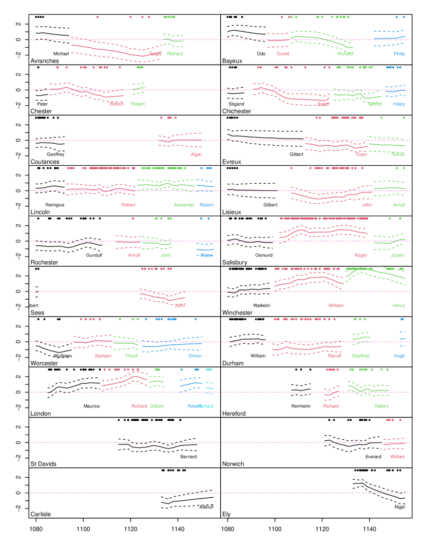
Figure 11: Bishop-authority curves $\bar{U}^{(t)}_{j}$ (solid curves) plotted for each bishop $j\in{\mathcal{M}}$ as a function of time from $b_{j}$ to $e_{j}$ with uncertainty at one-sigma. The dots at the top of each graph show the times of lists in which the color-matched bishop appeared. This is output from the constrained seniority effects analysis in Sec 6.3.

The continuity in authority (but not status) of bishops over time within a diocese in Fig 11 is noteworthy. There are some exceptions. For example, Henry de Blois started with higher authority than might be expected based only on the diocese. Some dioceses seem to be better (Winchester, London, Lincoln) than others (Chichester, Rochester, the dioceses in Normandy). The bishops of London and Winchester had gained precedence over their colleagues at the Council of London in 1075 and Lincoln came in the later middle ages to rank after Winchester. However, there is uncertain evidence from as early as 1138 that the bishop of Lincoln might assume the role of London or Winchester in their absence and consequently that Lincoln already enjoyed a degree of precedence (Johnson, 2013).

6.4 Discussion of results

From a historical perspective, there are three significant outcomes. The first is the strong emphasis on the seniority and precedence of individual bishops in the witness lists. Historians often link the relative position of witnesses to an assessment of their political significance, but the analysis here shows that royal scribes were strongly influenced by the rules on seniority and precedence expressed at the Council of London, held by the English church in 1075 (Council of London, 1075, clause 1, Clover and Gibson (1979)).

The second is the position of Normandy within the Anglo-Norman realm. Fig 11 shows that early in this period (before about 1100) Norman bishoprics enjoyed high status, but that this declined from the early twelfth century. This change is particularly marked for Avranches, Bayeux and Évreux, whilst no English bishoprics show a comparable trend. This should inform the ongoing debate about the relationship between England and Normandy (Bates (2013), chapter 5). This change might represent a principled decision by royal scribes to rank Norman bishops lower in precedence than their English counterparts, or it might be explained politically. The smaller Norman dioceses may have been less attractive to ambitious clergymen, and there were periods when Normandy and England were ruled separately (most notably, 1144-54), so that Norman bishops were external to the English kingdom.

The third concerns how far the behaviour of individual bishops could change their status. Bishops were active politically and could fall into disgrace. Thus, Bishop Nigel of Ely had high status for a junior bishop in the 1130s, but from his disgrace in 1139 his status fell, contrary to the usual pattern. Nigel’s pattern is unique; it is not replicated by that for other disgraced bishops, such as Ranulf Flambard of Durham after 1100 and Alexander of Lincoln after 1139. These differences presumably reflect the nature of the disgrace itself.

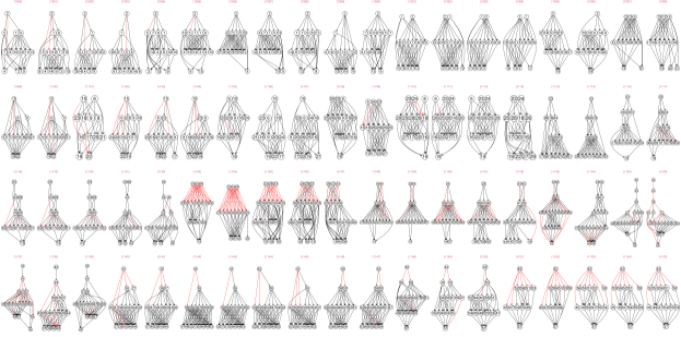
Figure 27: Consensus partial orders for all years 1080-1155 under the constrained-effects model of Sec H.3. These are transitive reductions. Edges have posterior support at least $\xi=0.5$. Red edges have support above $0.9$. Vertex numbering as Fig 9.

The estimated partial order relations are in line with what we expect in light of known political favour and the emphasis on seniority demonstrated here. For example, Henry of Blois and Odo of Bayeux, who were closely related to the royal house (Odo was William the Conqueror’s half-brother, and Henry was Stephen’s brother), are highly ranked. Referring to Fig 27 in Supp H.2, although Henry did well from the start, until 1135 he shares top spot in consensus orders with Roger of Salisbury. From this date he is promoted ahead of anyone else. This suggests that his brother becoming king in 1135 had an impact on his position.

The orders seem relatively shallow, with a group of middle-ranked bishops and a few above or below as typified by 1124 in Fig 27. We may be concerned that this reflects an overly informative prior and differences in how often bishops witness. We tested this by simulating synthetic data in which the true partial orders were total orders (see Supp L.2), but with the same list memberships as the real data. We reconstructed the true total orders well. If the true orders were total orders we would see this in our analysis.

7 Comparisons with other models

Drop time and consider a generic partial order $H\in{\mathcal{H}}_{\mathcal{A}}$ with ground set ${\mathcal{A}}$. When we fit partial orders to lists with an observation model like Eqn 3 we need to compute $|\mathcal{L}[H]|$, the linear extension count. This is intractable if $|{\mathcal{A}}|$ is at all large (about $20$ using our MCMC methods and hardware). In this section we define models over Bucket Orders and VSP orders (Valdes et al., 1982). Calculation of $|\mathcal{L}[H]|$ is linear in $|{\mathcal{A}}|$ on these subspaces of ${\mathcal{H}}$ (Wells, 1971), so if these models were preferred then we would use them. We find they are not adequate to represent a time-evolving hierarchy over long periods of time but can give a good fit over short time periods. Jiang et al. (2023) applies a fixed-time VSP model to all the witness list data (not just bishops). Some orders have over 200 actors, with lists exceeding 50 in length, and are out of reach for our analysis.

In Supp K.1 and K.2 we compare our model with Plackett-Luce models. Bayesian analysis of time-series Plackett-Luce in Supp K.1 gives similar results for a parameter function corresponding to the average authority $\bar{U}^{(t)}_{j}$ in Eqn 20. Analysis of a Plackett-Luce mixture model in Supp K.2 on short time intervals shows our model is preferred.

7.1 Bucket Orders and Vertex-Series-Parallel partial orders

VSP orders are built recursively from the ground set by taking series and parallel combinations of partial orders. Let ${\mathcal{A}}_{1},{\mathcal{A}}_{2}$ be disjoint sets of actor labels and let $a_{1}\in{\mathcal{H}}_{{\mathcal{A}}_{1}}$ and $a_{2}\in{\mathcal{H}}_{{\mathcal{A}}_{2}}$ be partial orders. Let

$$a_{1}\stackMath\mathbin{\stackinset{c}{0ex}{c}{0ex}{{}_{S}}{\bigcirc}}a =a_{1}\cup a_{2}\bigcup_{j_{1}\in{\mathcal{A}}_{1}\atop j_{2}\in{\mathcal{A}}_{2}}\{\langle j_{1},j_{2}\rangle\},$$

denote series combination setting all actors in $$a_{1} a_{2}$$ “above” those in and let

$$a_{1}\stackMath\mathbin{\stackinset{c}{0ex}{c}{0ex}{{}_{P}}{\bigcirc}}a_{2} =a_{1}\cup a_{2},$$

denote the parallel combination in which all actors in $a_{1}$ are unordered with respect to those in $a_{2}$. We now define the class ${\mathcal{V}}_{{\mathcal{A}}}$ of VSP orders on a general set ${\mathcal{A}}$ (Valdes et al., 1982):

1. For $j\in{\mathcal{A}}$ let ${\mathcal{V}}_{j}=\{\emptyset\}$ to be the empty order on a single actor $j$;

2. The class ${\mathcal{V}}_{{\mathcal{A}}}$ is the set of all partial orders $H$ which can be decomposed as $H=a_{1}\stackMath\mathbin{\stackinset{c}{0ex}{c}{0ex}{{}_{S}}{\bigcirc}}a_{2}$ or $H=a_{1}\stackMath\mathbin{\stackinset{c}{0ex}{c}{0ex}{{}_{P}}{\bigcirc}}a_{2}$ for some partition ${\mathcal{A}}_{1},{\mathcal{A}}_{2}$ of ${\mathcal{A}}$ and some $a_{1}\in{\mathcal{V}}_{{\mathcal{A}}_{1}}$ and $a_{2}\in{\mathcal{V}}_{{\mathcal{A}}_{2}}$.

A sequence of series or parallel combinations defining a given VSP is represented by a Binary Decomposition Tree (BDT, Valdes (1978)): leaves match elements of ${\mathcal{A}}$ and each internal vertex is an $\stackMath\mathbin{\stackinset{c}{0ex}{c}{0ex}{{}_{S}}{\bigcirc}}$ or $\stackMath\mathbin{\stackinset{c}{0ex}{c}{0ex}{{}_{P}}{\bigcirc}}$ operation on the VSPs rooted by its left and right child vertices. The BDT displayed in Fig 12 represents the partial order in Fig 1, which happens to be a VSP. The “plus” and “minus” symbols on the vertices below an $S$-vertex indicate the upper and lower VSP in a $\stackMath\mathbin{\stackinset{c}{0ex}{c}{0ex}{{}_{S}}{\bigcirc}}$-operation. Any given VSP may have many BDT representations (Jiang et al. (2023) counts them). If $H\in{\mathcal{V}}_{\mathcal{A}}$ is a VSP then $|\mathcal{L}[H]|$ can be computed in a time linear in $|{\mathcal{A}}|$ (Wells, 1971).

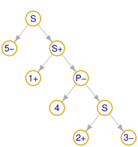
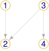
Figure 12: (left) BDT representation of the partial order in Fig 1. Working up from the bottom, 2 is above 3, 4 is unordered with respect to 2 and 3, 1 is above all three actors, and finally 5 is below all of 1-4. (right) The forbidden sub-graph $F$. A VSP order is any partial order which does not contain a sub-graph isomorphic to $F$.

The class of all VSPs ${\mathcal{V}}_{{\mathcal{A}}}$ is identical to the set of partials orders $H\in{\mathcal{H}}_{\mathcal{A}}$ which do not contain a set of vertices ${\mathcal{A}}^{\prime}=\{j_{1},...,j_{4}\}$ with sub-graph $H^{\prime}=H\cap({\mathcal{A}}^{\prime}\times{\mathcal{A}}^{\prime})$ that is isomorphic to the “forbidden subgraph” $F=\{\langle 1,2\rangle,\langle 3,2\rangle,\langle 3,4\rangle\}$ shown in Fig 12 at right (Valdes et al., 1982). After vertex relabelling, $F$ and $H^{\prime}$ must be identical, so edges absent in $F$ are absent in $H^{\prime}$. This makes it straightforward to test if a partial order $H$ is a VSP-order. VSP-orders are a small subset of partial orders. In our application with $|{\mathcal{A}}|\leq 18$ we have $|{\mathcal{H}}_{[18]}|\simeq 2\times 10^{35}$ and $|{\mathcal{V}}_{[18]}|/|{\mathcal{H}}_{[18]}\simeq 10^{-11}$ (OEIS Foundation Inc, 2022).

A sub-class of VSPs called “Bucket Orders” admits a simple closed form for its counts. In a Bucket Order, actors are grouped into “buckets”. Actors in the same bucket are unordered and a complete order holds over the buckets. Formally, if ${\mathcal{K}}_{\mathcal{A}}$ is the class of Bucket Orders on ${\mathcal{A}}$ then $b\in{\mathcal{K}}_{\mathcal{A}}$ iff there is a partition ${\mathcal{A}}_{1},...,{\mathcal{A}}_{P}$ of ${\mathcal{A}}$ into $P$ buckets such that for each $k\in[P]$ and all $j_{1},j_{2}\in{\mathcal{A}}_{k}$ we have $\langle j_{1},j_{2}\rangle\not\in b$ and for all pairs $1\leq k_{1}<k_{2}\leq P$ of buckets and all $j_{1}\in{\mathcal{A}}_{k_{1}}$ and $j_{2}\in{\mathcal{A}}_{k_{2}}$ we have $\langle j_{1},j_{2}\rangle\in b$. In our setting $|{\mathcal{K}}_{[18]}|/|{\mathcal{H}}_{[18]}|\simeq 10^{-17}$.

7.2 Bucket and VSP-order models

Suppose we are interested in learning about order relations over a period $[t_{1},t_{2}]$ with $B\leq t_{1}\leq t_{2}\leq E$. Recall that ${\mathcal{H}}^{(B,E)}$ in Eqn 7 is the space of partial order sequences $h=(h^{(B)},...,h^{(E)})$. If we could restrict the process of fitted partial orders $h\in{\mathcal{H}}^{(t_{1},t_{2})}$ to a VSP-order-process $h\in{\mathcal{V}}^{(t_{1},t_{2})}$ with

$${\mathcal{V}}^{(t_{1},t_{2})}={\mathcal{V}}_{{\mathcal{M}}_{t_{1}}}\times{\mathcal{V}}_{{\mathcal{M}}_{t_{1}+1}}\times...\times{\mathcal{V}}_{{\mathcal{M}}_{t_{2}}},$$

or a bucket-order process $h\in{\mathcal{K}}^{(t_{1},t_{2})}$ with

$${\mathcal{K}}^{(t_{1},t_{2})}={\mathcal{K}}_{{\mathcal{M}}_{t_{1}}}\times{\mathcal{K}}_{{\mathcal{M}}_{t_{1}+1}}\times...\times{\mathcal{K}}_{{\mathcal{M}}_{t_{2}}},$$

computation times would be vastly improved. However, this is hard to justify in our setting: there is no reason why the forbidden subgraph $F$ should not appear as a set of relations between bishops. Also, the data do not support this constraint. For example, the consensus order from 1137 in Fig 10 contains a sub-graph $H^{\prime}=\{\langle 35,48\rangle,\langle 47,48\rangle,\langle 47,38\rangle\}$, isomorphic to $F$, with each included edge having posterior probability 0.9 or above and absent edges below 0.5, so the true partial order is probably not a VSP.

7.3 Testing partial orders against restricted orders

In this section we consider data overlapping a time-window $[t_{1},t_{2}]$ by at least a half. Let

$$y^{(t_{1},t_{2})}=\left\{y_{i}:i\in{\mathcal{I}},\ \frac{1+\min(t_{2},\tau^{+}_{i})-\max(t_{1},\tau^{-}_{i})}{1+\tau^{+}_{i}-\tau^{-}_{i}}\geq 0.5\right\}.$$

denote this windowed data. Consider the Bayes factor

$$B_{{\mathcal{V}},{\mathcal{H}}} =\frac{p(y^{(t_{1},t_{2})}|h\in{\mathcal{V}}^{(t_{1},t_{2})})}{p(y^{(t_{1},t_{2})}|h\in{\mathcal{H}}^{(t_{1},t_{2})})},$$

with marginal likelihoods $p(y^{(t_{1},t_{2})}|h\in{\mathcal{V}}^{(t_{1},t_{2})})$ and $p(y^{(t_{1},t_{2})}|h\in{\mathcal{H}}^{(t_{1},t_{2})})$. Replace ${\mathcal{V}}$ with ${\mathcal{K}}$ to give $B_{{\mathcal{K}},{\mathcal{H}}}$ for Bucket Orders. Because the sets ${\mathcal{K}}^{(t_{1},t_{2})}\subset{\mathcal{V}}^{(t_{1},t_{2})}\subset{\mathcal{H}}^{(t_{1},t_{2})}$ are nested, these Bayes factors are easily estimated using Savage-Dickey estimators and MCMC samples from the full posterior $\pi(\rho,\theta,U,\beta,\tau,p|y^{(t_{1},t_{2})})$ in Eqn 17. We have

$$B_{{\mathcal{V}},{\mathcal{H}}} =\frac{\pi({\mathcal{V}}^{(t_{1},t_{2})}|y^{(t_{1},t_{2})})}{\pi({\mathcal{V}}^{(t_{1},t_{2})})},$$ (24)

where

$$\pi({\mathcal{V}}^{(t_{1},t_{2})}|y^{(t_{1},t_{2})})=E_{\rho,\theta,U,\beta,\tau,p|y^{(t_{1},t_{2})}}\left(\mathbb{I}_{h(Z(U,\beta;s))\in{\mathcal{V}}^{(t_{1},t_{2})}}\right)$$

is the posterior expectation and $\pi(h\in{\mathcal{V}}^{(t_{1},t_{2})})$ is the corresponding prior expectation.

7.4 Test results

We estimate Bayes Factors for twelve short (five-year) time intervals for accurate estimation of $\pi({\mathcal{V}}^{(t_{1},t_{2})})$ and $\pi({\mathcal{K}}^{(t_{1},t_{2})})$. We use the same time intervals for the Plackett-Luce analysis in Supp K.2. There is little change in seniority in these short time intervals (seniority-rank and bishop-label are colinear) so seniority effects were set to $\beta_{r}=0,\ r=1,...,S$ in the fitted partial order model. The likelihood $p_{(U)}$ in Eqn 5 was used. For analysis in interval $[t_{1},t_{2}]$, we take $K$, the dimension of $U^{(t)}_{j}$, to be $\lfloor\frac{1}{2}\max_{t\in[t_{1},t_{2}]}m_{t}\rfloor$. All other prior distributions are as summarised in Sec 2.4.

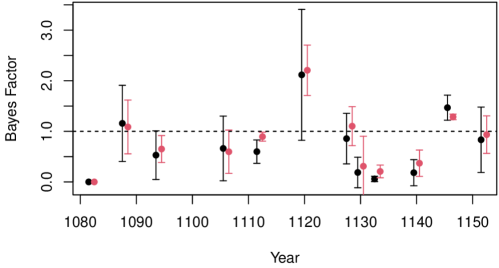
Figure 13: Bayes Factors for VSP orders (red) and Bucket Orders (black) fitted over the year intervals in Table 1. A value less than one is evidence against VSP or Bucket Orders. The $x$-axis value for each bar is the centre of the corresponding interval, $(t_{1}+t_{2})/2$. Error bars are two standard deviations.

Results are given in Table 1 in Supp J and plotted in Fig 13. Each point is an independent MCMC run. The prior probabilities $\pi(h\in{\mathcal{V}}^{(t_{1},t_{2})})$ and $\pi(h\in\mathcal{B}^{(t_{1},t_{2})})$ in Table 1 are surprisingly large given the sparsity of VSPs and Bucket Orders. This give insight on our prior for partial orders, which must promote VSPs and Bucket Orders. In retrospect, this is an acceptable representation of prior belief: the rules forming VSP-orders and Bucket Orders compare groups rather than actors and seem historically plausible; our process can leave the space of VSPs when the data demand it.

As Fig 13 shows, the data generally favour partial orders (or are neutral) except for the interval 1118-1122. We conclude that Bucket Orders and VSP models may be acceptable over some short time intervals, effectively “fixed time”. Experiments with longer time intervals (not reported) give more extreme Bayes factors rejecting VSP and Bucket Orders.

8 Conclusions

A new class of models for time series data listing rank data is summarised in Sec 2.4. The observation model in Eqn 16 was motivated by thinking of lists as realisations of a virtual queue in which the relative positions of actors are constrained by an underlying social hierarchy which we model as a partial order. We allowed for noise via the queue-jumping error model in Eqn 4. We gave a marginally consistent prior for the stochastic process of partial orders using the latent variable representation in Eqn 15. This made it straightforward to introduce a parameter controlling partial order depth and incorporate actor-covariates informing the position of actors in the hierarchy.

We fit the model to witness-list data in which the actors are eleventh and twelfth century bishops. In Sec 6.2 we saw that the model recovered structure in the data which was anticipated by historians. In particular, the dependence of the status of a bishop on their seniority is clear in Fig 8. We checked for evidence that the depth parameter $\rho$, correlation $\theta$ and error probability $p$ varied over time by looking at short time intervals (see Supp I) and found no evidence against our assumption of constant values over time. Further support comes from model comparison against a Placket-Luce mixture in Supp K.2 which favoured our model. The time-series extension of the Plackett-Luce model in Supp K.1 gave similar results for seniority effects and evolving authority, showing that the data overwhelm these model variations and conclusions are robust. The model is fairly time consuming to fit so there was no great gain in efficiency over partial orders on our data.

Having validated the model and fitting procedures, we gave our main analysis in Sec 6.3. This is the first quantitative analysis of these data and gave insights which historians find interesting. With few exceptions, witness-lists reflect precedence by diocese and seniority more than any sense of changing royal favour. We separated the effect of authority and seniority and confirmed (Johnson, 2013) that the bishops of London, Winchester and Lincoln had high authority and that Rochester had no special status. Personal authority does change in a few cases: the high status originally given to Nigel of Ely unwound over the course of his career, and Roger of Salisbury bucked the trend in Salisbury. This was well known to historians. The apparent decline in the authority of the Norman bishops (at least as far as it is expressed in the lists) was unknown to historians.

There is work to be done in computation, methodology and historical analysis. First, our MCMC is time consuming (the experiments in this paper add up to about two years of MCMC if run as a single serial process). Whilst a careful analysis minimising any approximation of the target distribution is justified (the data took time to compile, and there will never be any more for this period), scalable methods would be welcome, and VSP-orders may be an acceptable compromise from a modelling perspective. This may allow us to fit more complex noise models and do “top-$k$” ranking, where we focus on the top $k$ actors in a larger hierarchy. Analysis of lists including lay witnesses as in Jiang et al. (2023) require scalable methods in order to count linear extensions in partial orders over hundreds of elements. Second, statistical tools for selecting the number of features $K$ in the status vector of a bishop would help automate analysis and remove the need for the kind of robustness check we did in Supp H.3. Third, a small number of other covariates beside seniority are available in the data and might be explored in model elaboration.

From a historical perspective this study raises several questions. Complex precedence structures seem to have existed, but how were they known? Was there some kind of precedence handbook, or other means of transmission? Comparisons between patterns of precedence relations in pre-conquest lists and lists from later periods might be revealing. Later documents are more accurately dated and so a more fine-grained analysis may be possible. Finally, there are forgeries among acta of this period. Cases that go against the usual pattern may be an indicator of forgery.

Software used to carry out the analysis presented in this paper are available at

$$\verb|https://github.com/gknicholls/Partial-order-HMM|.$$

and

Appendix A Data registration

A.1 Data sources and data-collection

The process behind the making of this dataset is complex. The acta were written by royal scribes, usually clergymen with legal training and political skill. Most were written at the behest of individuals or institutions who wanted to obtain rights or privileges or ensure the intervention of royal agents in their favour. The scribes handed over the documents to these individuals or institutions, and they were responsible for preserving them. There was no central governmental archive until the 1190s, so there were no copies kept at Westminster or elsewhere.

Over time, many acta were destroyed accidentally or purposefully; those which survive tend to come from institutions such as towns or great churches which had a stable existence over centuries, and which had the capacity to protect and manage an archive. The activities of manuscript collectors has also had a significant impact on what has survived. The acta are now mostly in the possession of the major research libraries and archives, with a small number in private hands.

Over the last century and a half, researchers have worked to identify where these documents survive, and to obtain transcripts of them. Editions and catalogues have been made from those collections (Davis and Whitwell, 1913; Johnson and Cronne, 1966; Cronne and Davis, 1968; Bates, 1998), and, more recently, databases (Sharpe et al., 2014). These are widely used by researchers and scholars and are key resources for major questions in political, social and cultural history.

A.2 Data registration

Our registration aimed to ensure that the data conformed to the observation process we describe in the paper. We clip the uncertainty ranges of the lists $\tau^{-}_{i},\tau^{+}_{i},\ i\in I$ so that they lie within the range allowed by the bishops they list, that is, we impose

$$[\tau^{-}_{i},\tau^{+}_{i}]\subseteq\bigcap_{j=1}^{n_{i}}[b_{y_{j}},e_{y_{j}}].$$

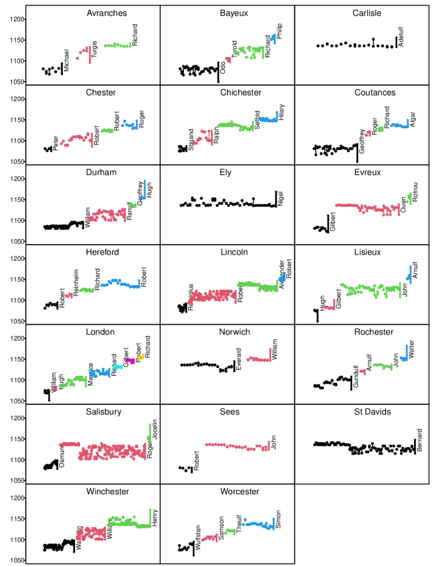
Figure 15: Each graph is a diocese with $y$-axis giving date in years. The $x$-axis is the index of lists by diocese. Each vertical line is a time interval. Thick lines (with an associate name) give time-interval in post for the named bishop. Thin lines give time intervals for lists. Some of these intervals are one year and are represented by a dot. Each bishop appear in the lists preceding that bishop. These share the same color. The possible date range of these lists is restricted to lay within the interval of time over which the bishop was active.

This is shown in Fig 15. This can lead to lists being dropped. For example, the list with data-set id 677 (see below), which has a data-set year indicator of 1139 (with no uncertainty), contains Philip, Bishop of Bayeux. He was in post 1142-1163 so the uncertainty range would be clipped to the empty set. The list with data-set id 2627 has both Hugh and John, bishops of Lisieux, with an obvious second list appended, starting with Henry I. These issues could be easily fixed. However, we simply dropped lists of this sort as the number was small (five).

The list with data-set id 2364 is a fairly typical example of a witness list we retained. The bishops do not quite appear as a group, as Ranulf is ahead of Maurice. We extract the sub-list of bishops in positions $3,4,5,6,7,9$ and code them as numbers using the table in Fig 24 yielding the registered list $Y=(18,16,27,25,9,15)$.

List id 2364

Year range [1107,1108], Witness List: [1] Matilda II, wife of Henry I, queen of England; [2] Anselm,, abbot of Bec, archbishop of Canterbury; [3] Robert, Bloet, bishop of Lincoln; [4] Robert, de Limesey, bishop of Chester; [5] John, Bishop of Lisieux; [6] Richard, Bishop of Bayeux; [7] Gundulf, bishop of Rochester; [8] Ranulf, chancellor of Henry I; [9] Maurice, bishop of London; [10] William, de Roumare, earl of Lincoln 1140; [11] Robert, II, count of Meulan; [12] David, King of Scots; [13] Robert, de Ferrers, earl of Derby.

List id 2627

Year range [1130,1135], List: [1] Odo, Stigandus; [2] Osmund, Boenot; [3] Serlo, de Mansione, Malgerii; [4] William, de Mirebel; [5] Hugh, Buscard; [6] Ranulf, de Iz; [7] Grento, de Vals; [8] Ralph, de Vals; [9] William I, king of England; [10] John, archbishop of Rouen; [11] Hugh, bishop of Lisieux; [12] Michael, bishop of Avranches; [13] Durand, abbot of Troarn; [14] Ainard, abbot of St Mary’s, Dives; [15] Nicholas, abbot of St Ouen; [16] Roger, de Montgomery, earl of Shrewsbury; [17] Roger, de Beaumont; [18] William, de Breteuil, count; [19] Henry I; [20] Matilda II, wife of Henry I, queen of England; [21] John, Bishop of Lisieux; [22] Rabel, de Tancarville, chamberlain; [23] Thurstan, Archbishop of York; [24] Robert, earl of Gloucester; [25] William, de Warenne II, earl of Surrey d. 1138; [26] Robert, de Beaumont, earl of Leicester; [27] Payn, Peverel.

List id 677

Year range [1139,1139], Witness List: [1] Robert, Losinga, bishop of Hereford [2] Philip, Bishop of Bayeux [3] Roger, archdeacon of Fecamp, temp. Stephen [4] Walter, archdeacon of Oxford [5] Waleran, count of Meulan [6] Ingelram de Say, temp. Stephen [7] Walter, of Salisbury, temp. Stephen [8] Robert, de Vere [9] William, de Pont de, l’Arche.

A.3 Dioceses of interest

The data display bishops with 31 distinct diocese names: Lincoln, Durham, Chester, Sherborne, Winchester, Chichester, Bayeux, Lisieux, Evreux, Sees, Avranches, Coutances, Exeter, London, Rochester, Worcester, Salisbury, Bath, Thetford, Wells, Le Mans, Hereford, Bangor, Ely, St Davids, Norwich, Carlisle, St Asaph, Tusculum, the Orkneys and Llandaff. We focused on a subset of 20 dioceses, shown in black on the $y$-axis of Fig 3 with results reported in Fig 11. We call this restricted set the “dioceses of interest”.

A.4 Further processing

We extracted lists from the period of interest, including only lists with at least two bishops. We then removed any bishops from excluded dioceses, and any bishops who only appeared in a single list. Depending on the period $[t_{1},t_{2}]$ of interest, this could reduce an included list from length two to one and removing that list could reduce the number of lists a bishop appeared in. We repeated this thinning to convergence. For the period $[1080,1155]$ this gave $371$ lists and $59$ distinct bishops in the dioceses of interest.

A.5 Discussion of data registration

Using a focus-set of dioceses and removing bishops from lists in this way was done to help make the analysis more tractable. Long lists (above about 16) yield partial order suborders with a large ground set (many vertices). Counting linear extensions in MCMC is demanding. However, the dioceses and bishops removed are represented in few lists, so any bishop-specific estimates like $U_{j}$ would be very uncertain anyway. The prior is marginally consistent, so in this respect the analysis is unchanged. However, removing bishops from longer lists does remove information informing the parameters of the bishops remaining (in all the models we considered, including the partial order and Plackett-Luce models). If we start with a list $Y=(j_{1},...,j_{n})$ with $n$ large then this supports the edge $\langle j_{1},j_{n}\rangle$ relatively strongly. If the list is reduced to a list $(j_{1},j_{n})$ then the edge $\langle j_{1},j_{n}\rangle$ is more weakly supported. If we have two lists $(j_{1},j_{2})$ and $(j_{2},j_{3})$ then we have support for $\langle j_{1},j_{3}\rangle$. If we remove bishop $j_{2}$ then we loose this information. These examples suggest that dropping bishops makes our estimated partial orders less certain, and contain fewer order relations. However, dropping bishops can remove evidence against orders. If we have three lists $(j_{1},j_{2})$, $(j_{2},j_{3})$ and $(j_{3},j_{1})$ then there is evidence for no order between $j_{1}$ and $j_{3}$. If we remove $j_{2}$ then we are left with evidence for the order $\langle j_{3},j_{1}\rangle$.

Considering the full 76 year period $[B,E]$, if we keep all lists overlapping the period with at least two bishops, and keep all dioceses and bishops we have 376 lists and 77 bishops. Restricting to dioceses of interest and bishops in at least two lists we have 371 lists and 59 bishops. The number of bishops drops significantly, which is helpful, but the number of lists hardly changes. Ninety percent of the lists remaining do not change at all, eight percent loose one member. We felt the change was sufficiently small it could be ignored and have not investigated further.

Appendix B Properties of priors

B.1 Proof of Proposition 1

We begin by stating the property that makes all this work.

Proposition 3.

The random partial order processes obtained by mapping the full $Z$-process to a partial order process and removing $j\in{\mathcal{M}}$ from each partial order in which it appears (“at the end”), or removing $j$ from the $Z$-process (“from the beginning”) are equal, so $h(Z^{(t)}_{-j})=h(Z^{(t)})[{\mathcal{M}}^{-j}_{t}\}]$ for $t\in[B,E]$.

Proof.

This follows from the fact that the relations $\langle j_{1},j_{2}\rangle$ in $h$ determined by Eqn 10 are not affected by the presence or absence of a third element $j$. ∎

Proposition 1. Let $g\in{\mathcal{H}}^{(B,E)}_{-j}$ be given. The prior in Eqn 18 is marginally consistent, that is

$$\pi_{{\mathcal{H}}^{(B,E)}_{-j}}(g|\beta=0_{S_{b}})=\sum_{h\in{\mathcal{H}}^{(B,E)}}\mathbb{I}_{g=h_{-j}}\pi_{{\mathcal{H}}^{(B,E)}}(h|\beta=0_{S_{b}}).$$

for each $j\in{\mathcal{M}}$.

Proof.

Marginal consistency follows from Proposition 3 using a Chinese Restaurant Process style construction. Let ${\mathcal{M}}=\{j_{1},...,j_{M}\}$ (labelling in any order). Add each “customer” $j_{1},...,j_{M}$ one at a time, using the fact that the $Z_{j}$-processes are jointly independent for $j\in{\mathcal{M}}$.

1. Initialise:

   1. Fix $K\geq 1$, simulate $(\rho,\theta)\sim\pi(\rho,\theta)$ and set $\beta=0_{S_{b}}$.

   2. For $t\in[B,E]$ set ${\mathcal{M}}_{t,1}=\{j_{1}\}\cap{\mathcal{M}}_{t}$, $h^{(t)}_{(1)}=\emptyset$ and simulate $Z_{j_{1}}\sim\mbox{VAR}^{(b_{j_{1}},e_{j_{1}})}_{K,\rho,\theta}(1)$ (recall $\beta=0_{S_{b}}$).

2. For $i=2,...,M$ do

   1. Simulate $Z_{j_{i}}\sim\mbox{VAR}^{(b_{j_{i}},e_{j_{i}})}_{K,\rho,\theta}(1)$.

   2. For $t\in[B,E]$ set ${\mathcal{M}}_{t,i}=\{j_{1},...,j_{i}\}\cap{\mathcal{M}}_{t}$ and construct $h^{(t)}_{(i)}$ by adding to $h^{(t)}_{(i-1)}$ the order relations between $j_{i}$ and $j_{1},...,j_{i-1}$, as follows: For $j\in\{j_{1},...,j_{i-1}\}$ the order relation $\langle j_{i},j\rangle$ (resp. $\langle j,j_{i}\rangle$) is added if $Z^{(t)}_{j_{i},k}>Z^{(t)}_{j,k}$ (resp. $Z^{(t)}_{j,k}>Z^{(t)}_{j_{i},k}$) for each $k=1,...,K$.

3. Set $h^{(t)}=h^{(t)}_{(M)}$ for each $t\in[B,E]$ and $h=(h^{(t)})_{t=B}^{E}$.

The final partial order time-series $h\sim\pi_{{\mathcal{H}}^{(B,E)}}(\cdot|\beta=0_{S_{b}})$ does not depend on the order in which the customers $j_{1},...,j_{M}$ arrive so we may make $j_{M}=j$ the last arrival. Also, by Proposition 3, $g=h^{(t)}_{-j}=h^{(t)}_{(M-1)}$ is the partial order state of the process for each $t\in[B,E]$ before $j_{M}=j$ arrives. By construction, $g\in{\mathcal{H}}^{(B,E)}_{-j}$ and $g\sim\pi_{{\mathcal{H}}^{(B,E)}_{-j}}(\cdot|\beta=0_{S_{b}})$. If we stop the process at step $i=M-1$ then the partial order we obtain must be the marginal over all continuations of the process to the next step, giving Proposition 1. ∎

Every partial order $h^{(t)}_{(i)},\ i=1,...,M-1$ is a suborder of the partial orders which come after it in the customer sequence, and adding or removing a customer does not change the order relations between other customers who have already arrived. This may be surprising, as we might expect new relations to add a cascade of relations by transitive closure. However,it is straightforward, as the relation between $Z_{j_{1}}$ and $Z_{j_{2}}$ in Eqn 10 isn’t affected by the presence or absence of $Z_{j_{3}}$.

B.2 Proof of Proposition 2

In this section we prove the universal expression property claimed in Sec 3.2.

Proposition 2. Suppose $\min_{t\in[B,E]}m_{t}\geq 4$. The probability $\pi_{{\mathcal{H}}^{(B,E)}}(h)$ in Eqn 19 given by the generative model Eqn 15 with $K\geq\lfloor S_{m}/2\rfloor$, assigns a positive probability mass $\pi_{{\mathcal{H}}^{(B,E)}}(h)>0$ to every timeseries $h\in{\mathcal{H}}^{(B,E)}$.

Before giving a proof we note that the condition $\min_{t\in[B,E]}m_{t}\geq 4$ requires the number of active actors to always exceed four. This condition is needed for Hiraguchi’s Theorem to hold. See Hiraguchi (1951) for the original result and Bogart (1973) for an accessible proof and discussion. In our application in Sec 5 $m_{t}\geq 11$ so the condition is satisfied.

Proof.

We first show that (1) every partial order in the time-series $h$ has dimension at most $K$. A total order is a partial order in which every pair of elements is ordered. The intersection of $K$ total orders $\ell=(\ell^{(1)},...,\ell^{(K)})$ on the ground set $[m]$ is a partial order $H=\cap_{k=1}^{K}\ell^{(k)}$ on $m$ elements satisfying $H\in{\mathcal{H}}_{[m]}$. A given partial order may be decomposed into total orders in many different ways (and always at least one, Dushnik and Miller (1941)). For example, the partial order $H$ in Fig 1 has three linear extensions, $Y^{(1)}=(1,2,3,4,5),Y^{(2)}=(1,2,4,3,5)$ and $Y^{(3)}=(1,4,2,3,5)$. We can turn these into total orders in the obvious way, setting $\ell^{(i)}=\{\langle Y^{(i)}_{j},Y^{(i)}_{j^{\prime}}\rangle\in Y^{(i)}\times Y^{(i)}:j<j^{\prime}\},\ i=1,2,3$. Then $H$ is both $H=\ell^{(1)}\cap\ell^{(3)}$ and $H=\ell^{(1)}\cap\ell^{(2)}\cap\ell^{(3)}$.

The dimension of a partial order $\dim(H)$ is the smallest number of total orders that intersect to give $H$. It is known (Hiraguchi, 1951) that if $H\in{\mathcal{H}}_{[m]}$ then $\dim(H)\leq\lfloor m/2\rfloor$. Restoring time to the notation, since $S_{m}=\max_{t}m_{t}$, we can take any $K\geq\lfloor S_{m}/2\rfloor$ and be sure that $\dim(h^{(t)})\leq K$ for every $t\in[B,E]$ and all $h\in{\mathcal{H}}^{(B,E)}$, where ${\mathcal{H}}^{(B,E)}$ (defined in Eqneq:h-sequence-space-defn) is the set of all possible partial order timeseries $h=(h^{(B)},h^{(B+1)},\ldots,h^{(E)})$ on the sequence of ground sets ${\mathcal{M}}_{B},{\mathcal{M}}_{B+1},\ldots,{\mathcal{M}}_{E}$.

We next show that (2) the mapping $h^{(t)}=h(Z^{(t)})$ takes the intersection over columns of the rank order for each column of $Z^{(t)}$. Consider a $m_{t}\times K$ matrix $Z^{(t)}$ in a particular year $t\in[B,E]$. The rule mapping $Z^{(t)}$ to $h^{(t)}$ in Eqn 10 just takes the intersection of the rank orders of the columns of $Z^{(t)}$: for $k=1,...,K$, the rank order in column $k$ is

$$\ell^{(t,k)}=\{\langle i,j\rangle\in{\mathcal{M}}_{t}\times{\mathcal{M}}_{t}:Z^{(t)}_{i,k}>Z^{(t)}_{j,k}\}$$

so Eqn 10 is the same as

$$h(Z^{(t)})=\cap_{k=1}^{K}\ell^{(t,k)}.$$

Write $\ell^{(t)}=(\ell^{(t,k)})_{k=1}^{K}$ for the $K$ total orders and write $\ell^{(t)}=\ell(Z^{(t)})$ to show that $\ell^{(t)}$ is determined from $Z^{(t)}$.

We next show (3) for any partial order time-series $h$ there is a set of latent variable time-series $Z$ each realising $h$. The set has non-zero measure. We realise any particular time-series $h\in{\mathcal{H}}_{[A,B]}$ if we realise $Z$ such that $h(Z)=h$, so we realise $h$ if we realise a sequence of $Z^{(t)}$-matrices with column rank orders $\ell^{(t)}=\ell(Z^{(t)})$ that intersect to give $h^{(t)}$. Since $\dim(h^{(t)})\leq K$ we know that such a sequence of rank orders exists, so we get $h$ with positive prior probability if the probability to realise such a $Z$ is positive.

The prior for $Z$ is given in terms of a continuous mixture (over $\rho$ and $\theta$) of multivariate normal $U$ and $\beta$ prior densities. It has a density with respect to Lebesgue measure on the space

$${\mathcal{Z}}^{(B,E)}=\mathbb{R}^{Km_{B}}\times\mathbb{R}^{Km_{B+1}}\times...\times\mathbb{R}^{Km_{E}}$$

which is strictly positive for all $Z\in{\mathcal{Z}}^{(B,E)}$ (so every possible sequence of $Z$-matrices can be realised). Let $h\in{\mathcal{H}}^{(B,E)}$ be given and let $\ell^{(t)}$ be any decomposition of $h^{(t)}$ into $K$ total orders (at least one decomposition exists, and if $\dim(h^{(t)})<K$ then we just repeat total orders as this does not change their intersection). Let

$${\mathcal{Z}}_{t,\ell}=\{z\in\mathbb{R}^{Km_{t}}:\ell(z)=\ell^{(t)}\}$$

be the set of $Z$-matrices in $\mathbb{R}^{Km_{t}}$ representing year $t$ that yield the desired column rank orders.

The sets ${\mathcal{Z}}_{t,\ell}$ are not empty: we can take the $m_{t}$ entries in the $k$’th column $Z^{(t)}_{{\mathcal{M}}_{t},k}=(Z^{(t)}_{j,k})_{j\in{\mathcal{M}}_{t}}$ of $Z^{(t)}$ to be any set of real numbers that match the column rank order constraint imposed by $\ell^{(t,k)}$. It follows that the volume measure of ${\mathcal{Z}}_{t,\ell}$ is strictly greater than zero.

Any $z\in{\mathcal{Z}}_{t,\ell}$ satisfies $h(z)=h^{(t)}$. However $\ell^{(t)}$ above is just one decomposition of $h^{(t)}$ into $K$ (not necessarily distinct) total orders, so $Z_{t,\ell}$ will typically be smaller than the set of all $z$’s giving $h^{(t)}$. Let

$${\mathcal{Z}}(h^{(t)})=\{z\in\mathbb{R}^{m_{t}K}:h(z)=h^{(t)}\}$$

be that set, with ${\mathcal{Z}}(h^{(t)})\supseteq{\mathcal{Z}}_{t,\ell}$. Let

$${\mathcal{Z}}(h)={\mathcal{Z}}(h^{(B)})\times{\mathcal{Z}}(h^{(B+1)})\times...\times{\mathcal{Z}}(h^{(E)}),$$

and

$${\mathcal{Z}}_{\ell}={\mathcal{Z}}_{B,\ell}\times{\mathcal{Z}}_{B+1,\ell}\times...\times{\mathcal{Z}}_{E,\ell}$$

so that again, ${\mathcal{Z}}(h)\supseteq{\mathcal{Z}}_{\ell}$ and the measure of ${\mathcal{Z}}_{\ell}$ is not zero.

Finally, (4) the prior probability to realise any time-series $h\in{\mathcal{H}}^{(B,E)}$ is not zero. Indeed,

$$\pi_{{\mathcal{H}}^{(B,E)}}(h) =\Pr(Z\in{\mathcal{Z}}(h))$$

$$\geq\Pr(Z\in{\mathcal{Z}}_{\ell})$$

$$>0,$$

as the density of $Z$ is not zero on the set ${\mathcal{Z}}_{\ell}$ and this set has non-zero measure. ∎

Appendix C Computational methods

C.1 Counting Linear extensions

In this Supp, which picks up from Sec 2.2.2, we outline how we count linear extensions of a given partial order $H\in{\mathcal{H}}_{[m]}$.

Recall from Sec 2.2.2 that $C(H)$ is the number of linear extensions of partial order $H$ and $C_{j}(H)$ is the number that start with $j$. If ${\mathcal{T}}(H)=\{j\in[m]:C_{j}(H)>0\}$ is the set of “top elements” of $H$ then

$$C(H)=\sum_{j\in{\mathcal{T}}(H)}C_{j}(H).$$

This is computed using a suborder recursion. If $j\in{\mathcal{T}}(H)$ and we let

$$H_{-j}=H[[m]\setminus\{j\}]$$ (25)

give the partial order $H$ with vertex $j$ removed then $C_{j}(H)=C(H_{-j})$, so we can prune away the vertices one at a time, starting at the top of the partial order. The count is available in closed form (or rapidly) for some subclasses of partial orders including the Bucket Orders and vertex-series-parallel orders described below. For example, the empty partial order, with $H=\emptyset$, has $C(H)=m!$. We implemented a simple R program using a recursion which terminates at these “easy” cases. We have also faster code based on Kangas et al. (2019) which we used in later work. Links to these are shared in our online code.

Appendix D Intersection orders

“Intersection orders” are obtained from total orders (which need not all have the same ground set) by taking all the relations which are attested by a set of lists and not contradicted. In order to compute an intersection order $\hat{h}^{(t)}$ in year $t$ we took the year for each list (which is sometimes uncertain) $\hat{\tau}_{i}=(\tau^{-}+\tau^{+})/2$ to be the centre year in its confidence range. We used lists in a sliding window $[t-w,t+w]$ covering $2w+1$ years. We took $w=2$.

For $i\in{\mathcal{I}}$ let $y^{(i)}=\{\langle y_{i,j},y_{i,j^{\prime}}\rangle\in y_{i}\times y_{i}:j<j^{\prime}\}$ be the total order derived from a list by setting all higher placed list elements above lower placed elements. Let ${\mathcal{I}}_{t,w}=\{i\in{\mathcal{I}}:t-w\leq\hat{\tau}_{i}\leq t+w\}$ give the labels for lists in the window and let

$$y^{{\mathcal{I}}_{t,w}}=\bigcup_{i\in{\mathcal{I}}_{t}}y^{(i)}$$

include all the order relations attested by lists in the window. The intersection order is

$$\hat{h}^{(t)}=\{\langle j,j^{\prime}\rangle\in y^{{\mathcal{I}}_{t,w}}:\langle j^{\prime},j\rangle\not\in y^{{\mathcal{I}}_{t,w}}\}.$$

Intersection orders are maximum likelihood estimates for the noise-free likelihood in Eqn 3 if all the list-data $y_{i},\ i\in{\mathcal{I}}_{t,w}$ contributing to a given order-estimate has the full length of the partial order in that year (Beerenwinkel et al., 2007) so $n_{i}=m_{t}$ for each $i\in{\mathcal{I}}_{t,w}$. In this special case $\hat{h}^{(t)}=\cap_{i\in{\mathcal{I}}_{t,w}}y^{(i)}$, hence the name.

We computed intersection-order estimates $\hat{h}^{(t)}$ for the years $t\in[1136,1138]$ and plot them in Fig 16. We do not use these, except for initialising MCMC, as our lists have variable length, so they have no statistical properties of value to us.

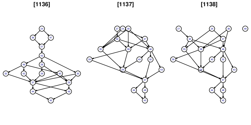
Figure 16: Intersection-order estimates (defined in Supp D) for a subset of years. The point estimate for a given year displays all the order relations displayed and not contradicted in the lists in a five year window centred on that year.

Appendix E Prior and Posterior depth distributions

In this section we report some summaries from prior simulation of depth distributions and compare them with posterior depth distributions. We have said that we would like prior depth distributions to be reasonably uniform. In Fig 17 we plot prior depth distributions. There is one curve for each of the $T=E-B+1=76$ years showing the prior depth distribution for that year. The two plots show distributions for $K=9$ and $K=18$ (left and right respectively).

In Sec 2.3.3 we mentioned that the uniform prior on partial orders $H\sim\mbox{Unif}({\mathcal{H}}_{[m]})$ concentrates on partial orders of depth three as $m\to\infty$ (Kleitman and Rothschild, 1975). We illustrate that along with the depth distributions of our priors. In Fig 17 (left and right), the dashed curve shows the prior depth distribution determined by the uniform prior. A random partial order $H\sim\mbox{Unif}({\mathcal{H}}_{[m]})$ simulated using the MCMC algorithm given in Muir Watt (2015) is shown in Fig 20. This illustrates the rather dramtic weighting present in this prior.

Our own prior distributions tend to rule out partial orders of depth 1 and are otherwise reasonably flat, weighting somewhat in favour of lower depth. Taking $K=18$ raises the prior probability for depth 1 slightly. This is hard to see in Fig 17 but visible in the left panels in Figs 18 and 19. Fig 18 shows prior and posterior depth distributions for the analysis in Sec 6.3 with $K=9$. We see that the whiskers do not extend to depth 1 in all years in the prior plot at left. Fig 19 shows prior and posterior depth distributions for the analysis in Supp H.3 which is the same as that in shown in Fig 18 except that $K=18$. We see that the whiskers do now extend to depth 1 in all years in the prior plot at left.

The prior we have given has reasonably flat support over depths that the data actually supports. We may be concerned that the depths with highest posterior probability in Figs 18 and 19 coincide with relatively higher prior-probability depths in Fig 17 (so, around 2-5). However, this is not prior domination. The data easily dominates the prior. We show this in Supp L.2 where we take synthetic data with the same list content (so the same $o_{i},\ i\in{\mathcal{I}}$ as the real data, but simulated data $y^{\prime}_{i},\ i\in{\mathcal{I}}$). We take “true” partial orders which are complete (or near complete) orders so the true depth is around $m_{t},\ t\in[B,E]$ for each year. We show we reconstruct this depth well, so the prior is in no way dominating the reconstructed depth. At the end of Supp L.2 we remark on the corresponding issue of potential prior bias at depth 1.

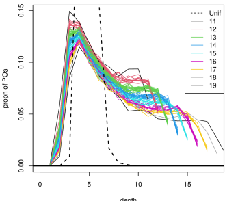
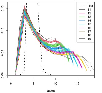
Figure 17: Monte-Carlo estimates of the depth distribution for the partial order at each time - using the prior for $h$ summarised in Sec 2.4: (Left) $K=9$ columns in the $Z$-matrix; (Right) $K=18$. This distribution varies as the number of bishops (indicated by color) in the partial order varies over time. The dashed curve is the depth distribution for a uniform partial order with $m_{t}=18$.

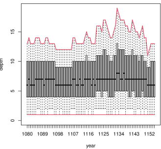
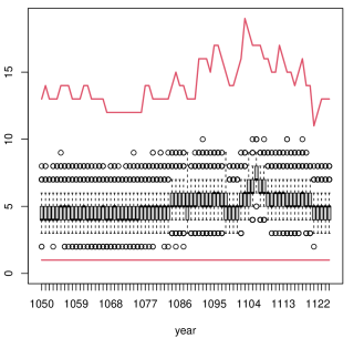
Figure 18: (Left) Prior and (Right) posterior depth distributions from the analysis in Sec 6.3 with $K=9$. The x-axis shows years. Each box represents the posterior distribution for its year. It is computed using prior samples (at Left) and MCMC posterior sample depths (at Right). The red lines indicate the least (equal one) and greatest (equal $m_{t}$ in year $t$) depth possible in a given year.

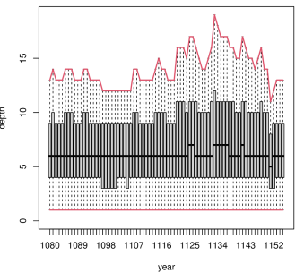
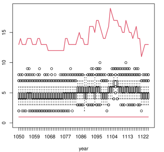
Figure 19: (Left) Prior and (Right) posterior depth distributions from the analysis in Supp H with $K=18$. Otherwise as Fig 18

Figure 20: A partial order on 50 nodes drawn approximately uniformly at random from ${\mathcal{H}}_{[50]}$ using the MCMC algorithm given in Muir Watt (2015), illustrating the concentration on orders of depth three.

Appendix F MCMC

Proposals for $\rho$ and $\theta$ (which are in $[0,1]$) are prior draws with a Hastings ratio which does not involve the final likelihood factor in Eqn 17. Candidate states $\beta_{r}\to\tilde{\beta}_{r},\ r=1,...,S_{b}$ for the components of $\beta\in\mathcal{B}_{0}$ or $\mathcal{B}_{S_{b}}$ are simple random walk proposals with a fixed bandwidth (rejecting if the order condition in $\mathcal{B}_{S_{b}}$ is violated).

Proposals for the $\mbox{VAR}^{(b_{j},e_{j})}_{K,\rho,\theta}(1)$ time series $U$ for each component $j\in{\mathcal{M}}_{t}$ target each time $t\in[b_{j},e_{j}]$ in turn. The candidate state $\tilde{U}^{(t)}_{j}\in\mathbb{R}^{K}$ is a draw from the prior conditioned on $\rho$ and $\theta$ and the values $U^{t-1}_{j},U^{t+1}_{j}$ of the process before and after the target vector, so that

$$\tilde{U}^{(t)}_{j} \sim N\left(\frac{\theta}{1+\theta^{2}}(U^{(t-1)}_{j}+U^{(t+1)}_{j}),\frac{1-\theta^{2}}{1+\theta^{2}}\Sigma^{(\rho)}\right),\ \mbox{if $b_{j}<t<e_{j}$},$$

$$\tilde{U}^{(b_{j})}_{j} \sim N\left(\theta U^{(b_{j}+1)}_{j},(1-\theta^{2})\Sigma^{(\rho)}\right),\ \mbox{if $t=b_{j}<e_{j}$},$$

$$\tilde{U}^{(e_{j})}_{j} \sim N\left(\theta U^{(e_{j}-1)}_{j},(1-\theta^{2})\Sigma^{(\rho)}\right)\ \mbox{if $b_{j}<t=e_{j}$},$$

$$\tilde{U}^{(t)}_{j} \sim N\left(0_{K},\Sigma^{(\rho)}\right)\ t=b_{j}=e_{j}$$ if

with special cases at the start and end of the active period for bishop $j$. This determines the candidate state $\tilde{U}$ (which differs from $U$ at just a single vector $U^{(t)}_{j}\to\tilde{U}^{(t)}_{j}$).

At $U$ and $\beta$ updates we update $\tilde{Z}=Z(\tilde{U},\beta;s)$ and $\tilde{Z}=Z(U,\tilde{\beta};s)$ respectively to determine the candidate partial order $\tilde{h}=h(\tilde{Z})$. In a $U$-update at year $t$, the partial order series $h$ and $\tilde{h}$ are equal except for the replacement $h^{(t)}\to\tilde{h}^{(t)}$ so cancellations leave the Hastings ratio depending on the likelihood for lists ${\mathcal{I}}_{t}(\tau)=\{i\in{\mathcal{I}}:\tau_{i}=t\}$ only. The acceptance probability is

$$\alpha(\tilde{U}^{(t)}|U^{(t)})=\min\left\{1,\ \prod_{i\in{\mathcal{I}}_{t}(\tau)}\frac{p(y_{i}|\tilde{h}^{(t)}[o_{i}],p)}{p(y_{i}|h^{(t)}[o_{i}],p)}\right\}.$$

Updates to components of $\beta$ affect $Z$ over all times so the full likelihood ratio is needed.

Proposals for $\tau$ are prior draws. The Hastings ratio depends only on likelihood factors for the list $i\in{\mathcal{I}}$ for which the date $\tau_{i}$ is being updated. If $\tilde{\tau}_{i}$ is the candidate value then the acceptance probability is

$$\alpha(\tilde{\tau}_{i}|\tau_{i})=\min\left\{1,\ \frac{p(y_{i}|h^{(\tilde{\tau}_{i})}[o_{i}],p)}{p(y_{i}|h^{(\tau_{i})}[o_{i}],p)}\right\}$$

Proposals for $p$ are also prior draws. This time the Hastings ratio is the full likelihood ratio, $p(y|h,\tau,\tilde{p})/p(y|h,\tau,p)$.

MCMC runs were initialised at either disordered or ordered initialisations. In the disordered initialisation all parameters were given starting values as far as possible from equilibrium values, the effects $\beta=0_{S_{b}}$, the times $\tau$ are prior draws subject to $\tau\in[B,E]^{N}$ and the $U$-matrices specified so that the order was empty (all paths cross in each year). In the ordered initialisation parameters start at values that might be typical for equilibrium, the effects $\beta$ and the lists times $\tau$ as for disordered, and the $U$-matrices specified so that the initial partial orders $h^{(t,0)}$ coincide with the “intersection orders” of the lists in each year $t=B,...,E$. Intersection orders are defined in Supp D. This choice ensures $h^{(t,0)}$ contains all the relations displayed by the lists and none contradicted by a list. We checked that two runs started in ordered and disordered initialisations gave the same posterior densities for marginal parameter posteriors. We checked effective sample sizes and inspected MCMC traces.

Appendix G Posterior summary statistics

G.1 Consensus Partial Order

We now define our principle posterior summaries. We seek a point estimate of the unknown true evolving status hierarchy of partial orders $h$. The consensus partial order with threshold $\xi\in[0,1]$ displays all the relations supported at time $t$ with estimated posterior probability

$$\hat{\xi}^{(t)}_{\langle j_{1},j_{2}\rangle}=L^{-1}\sum_{l=1}^{L}\mathbb{I}_{\langle i,j\rangle\in h^{(t,l)}}$$

greater than or equal $\xi$. It is a directed graph

$$\bar{h}^{(t)}(\xi)=(E_{t}(\xi),{\mathcal{M}}_{t})$$ (29)

on the active bishops in year $t$ with edges

$$E_{t}(\xi)=\left\{\langle j_{1},j_{2}\rangle\in{\mathcal{M}}_{t}\times{\mathcal{M}}_{t}:\hat{\xi}^{(t)}_{\langle j_{1},j_{2}\rangle}\geq\xi\right\}.$$

The consensus partial order need not be acyclic, even when $\xi\geq 0.5$, so $\bar{h}^{(t)}(\xi)\not\in{\mathcal{H}}_{t}$ is possible. This seems to be possible but improbable: all the consensus partial orders in this paper are partial orders.

G.2 Testing for an effect due to seniority

We estimate a Bayes factor for the seniority effects $\beta_{r},\ r=1,...,S$ to be decreasing with decreasing seniority (so increasing seniority-rank $r$). Let $\mathcal{B}_{S^{\prime}}=\{\beta\in\mathcal{B}_{0}:\beta_{1}>\beta_{2}>...>\beta_{S^{\prime}}\}$ be the event that the first $S^{\prime}\leq S_{b}$ effects are ordered. It is feasible to compare models with $\beta\in\mathcal{B}_{0}$ against $\beta\in\mathcal{B}_{S^{\prime}}$ for $S^{\prime}$ up to about $S^{\prime}=9$ using a Savage-Dickey estimator, as $\mathcal{B}_{S^{\prime}}\subset\mathcal{B}_{0}$. We have

$$B_{S^{\prime},0} =\frac{p(y|\beta\in\mathcal{B}_{S^{\prime}})}{p(y|\beta\in\mathcal{B}_{0})}$$

$$=\frac{\pi(\beta\in\mathcal{B}_{S^{\prime}}|y)}{\pi(\beta\in\mathcal{B}_{S^{\prime}})}$$ (30)

$$=S^{\prime}!\,E_{\rho,\theta,U,\beta,\tau,p|y}(\mathbb{I}_{\beta\in\mathcal{B}_{S^{\prime}}}),$$

as the marginals $\pi(\beta\in\mathcal{B}_{0}|y)=\pi(\beta\in\mathcal{B}_{0})=1$ for the unconstrained posterior $\pi(\rho,\theta,U,\beta,\tau,p|y)$, and $\pi(\beta\in\mathcal{B}_{S^{\prime}})=1/S^{\prime}!$. The expectation can be estimated using samples from $\pi(\rho,\theta,U,\beta,\tau,p|y)$. The point here is that the prior probability for $\beta\in\mathcal{B}_{S^{\prime}}$ is very small for $S^{\prime}$ at all large, so if we see any posterior samples with $\beta\in\mathcal{B}_{S^{\prime}}$ this shows the data is weighting strongly in favour of these configurations. However, even though we may have $\pi(\beta\in\mathcal{B}_{S^{\prime}}|y)\gg\pi(\beta\in\mathcal{B}_{S^{\prime}})$ the numerator in Eqn 30 is very small for large $S^{\prime}$ and hard to estimate accurately, so we restrict discussion to $S^{\prime}\leq 9$.

Appendix H Further results and comparison analyses

H.1 Additional figure for the analysis in Sec 6.2

Fig 22 shows MCMC traces for selected parameters and functions in the MCMC for the analysis in Sec 6.2 using the MCMC algorithm of Supp F. This paper contains results from dozens of MCMC runs so we present this as specimen output. Another specimen set of MCMC traces are given in Fig 32 in Supp L.1 where we analyse synthetic data with the same model and structure as in this section (obtaining good recovery of truth). For the main analyses in Sec 6.2 and 6.3 we ran two independent MCMC chains with different start states and obtained excellent agreement.

Fig 21 shows comparisons of posterior distributions for the parameters $\rho,\theta$ and $p$ for the unconstrained seniority-effects model $\beta\in\mathcal{B}_{0}$ (so, as Sec 6.2) across runs with different model settings. The prior for each parameter is also plotted (except $\theta$ which is uniform). These show good agreement across models. We vary the likelihood noise model ($p_{U}$ and $p_{(D)}$) and the number of columns $K$ in the status matrix $Z^{(t)}$. The serial-correlation parameter $\theta$ and the queue-jumping error probability $p$ are almost unchanged when these other aspects of the model are varied.

The $\rho$ posterior for $K=18$ (green curve in left panel) is shifted slightly towards one. This is because the “paths” (rows of $Z^{(t)}$) must be more strongly correlated than is the case for $K=9$ in order to get the same or similar typical partial order depth. When the paths are longer the hazard for them crossing is greater. This would remove order relations so they need to be flatter (and hence more strongly correlated) to get the same depth.

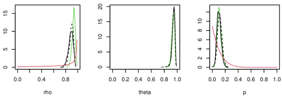
Figure 21: Posterior parameter densities for $\rho,\theta$ and $p$ from a selection of different models for the same data in the analysis of Sec 6.2. The priors are given in Sec 4.2 with $\beta\in\mathcal{B}_{0}$ and variations: (solid black line) $K=9$, likelihood $p_{(U)}$ in Eqn 5; (dashed black) $K=9$, likelihood $p_{(D)}$ in Eqn 4; (solid green) $K=18$, likelihood $p_{(U)}$. The red curve in the $\rho$ and $p$ graphs is their prior. The prior for $\theta$ is uniform.

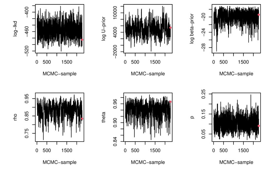
Figure 22: Selected MCMC traces from the unconstrained seniority-effect analysis in Sec 6.2.

H.2 Figures from the analysis in Sec 6.3

In this section we show some further results from the analysis presented in Sec 6.3, the analysis with constrained seniority effect parameters $\beta\in\mathcal{B}_{S_{b}}$ and $K=9$ columns in the status matrix $Z^{(t)}$.

In Fig 23 we show transitive closures of the consensus partial order $\bar{h}^{(t)}(\xi)$ defined in Eqn 29 for the years $t\in[1136,1138]$. Throughout this paper, edges with thresholds $\xi=0.5$ and $\xi=0.9$ are shown in black and red respectively. The reductions are shown in Fig 10. These transitively closed consensus partial orders are hard to read so we prefer reductions. We show them to emphasise that many well-supported relations (red edges) are found, as a sequence of weakly supported relations (black edges $\langle j_{1},j_{2}\rangle,\langle j_{2},j_{3}\rangle$) in the reduction tends to yield a well supported relation $\langle j_{1},j_{3}\rangle$ in the closure.

Fig 24 gives the mapping from names to numbers in all graphs in this paper.

Fig 25 shows the posterior mean status curves $\bar{Z}_{j}^{(t)},\ t\in[b_{j},e_{j}]$ for each bishop $j\in{\mathcal{M}}$. This is defined as for $\bar{U}_{j}^{(t)},\ t\in[b_{j},e_{j}]$ in Eqn 20. This figure should be compared with Fig 11. For further discussion of this pair of figures see Sec 6.3.

Fig 26 shows 90% HPD sets for the posterior distribution of the list times $\tau_{i},\ i\in{\mathcal{I}}$. The $x$-axis in this graph is the list index (sorted, so that prior mean list times increase). Recall the data gives us a time range $\tau_{i}\in[\tau_{i}^{-},\tau_{i}^{+}]$ for each list. The red bars show this time interval constraint, and also represent the prior, which is uniform. The dates of some lists are known without uncertainty (so $\tau_{i}^{-}=\tau_{i}^{+}$). These lists have been omitted from Fig 26. It can be seen that the data do inform the list times a little (the grey set is restricted relative to the red bar) though the benefit is seen mainly in lists with substantial prior time ranges (the longer red bars). The principle purpose of including the uncertain list dates in the analysis is to feed through the uncertainty in list dates into the estimates of average authority $\bar{U}^{(t)}_{j}$ and consensus partial orders $\bar{h}^{(t)}(\xi)$ rather than to do list dating.

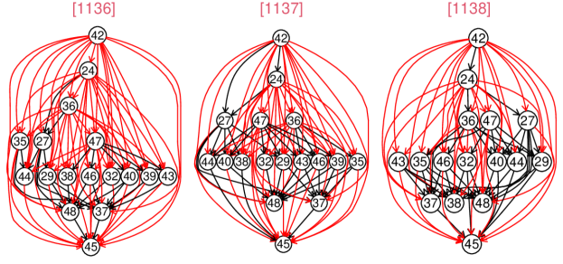
Figure 23: Consensus partial orders for the years 1136-1138 (a selection from the years 1080-1155) under the constrained-effects model of Sec 6.3. These are the transitive closures corresponding to the reductions in Fig 10 in Sec 6.3. Edges have posterior support at least $\xi=0.5$. Red edges have support above $0.9$. Vertex numbering as Fig 9.

Figure 24: Name index for vertices in the order graphs in Figs 9, 10, 16 and 23.

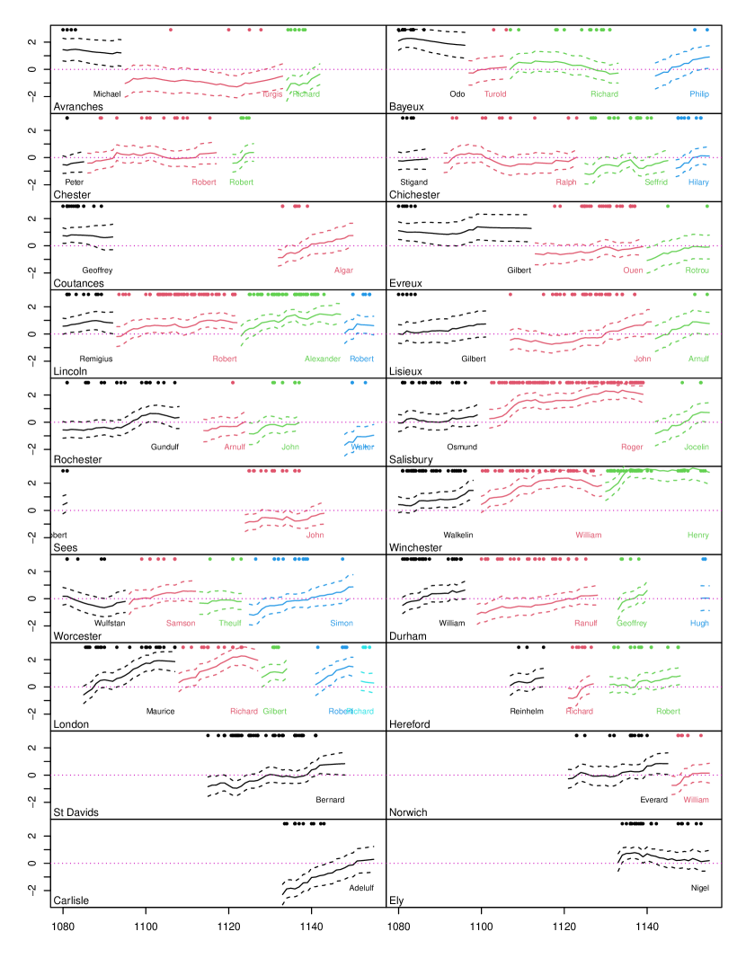
Figure 25: Bishop-status curves $\hat{Z}^{(t)}_{j}$ (solid curves) plotted for each bishop $j\in{\mathcal{M}}$ as a function of time from $b_{j}$ to $e_{j}$ with standard errors at one-sigma. The dots along the top of each graph show the times of the lists in which the color-matched bishop below appeared. This is output from the constrained seniority effects analysis in Sec 6.3.

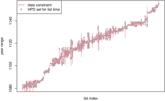
Figure 26: Posterior distributions of the unknown list times $\tau_{i},\ i\in{\mathcal{I}}$. Some lists have known times, shown are the posteriors for uncertain list times. The $x$-axis is the list index (sorted by prior mean time) and the $y$-axis is in years CE. The red line shows the known constrained interval $[\tau^{-}_{i},\tau^{+}_{i}]$ for each list. The grey region over each vertical line is a 90% HPD set for the estimated age of the associated list. This is output from the constrained seniority effects analysis in Sec 6.3.

H.3 Figures from an analysis like Sec 6.3 but with $K=18$.

Here we gather together results from an analysis identical to that in Sec 6.3 (constrained seniority effects, $\beta\in\mathcal{B}_{S_{b}}$) but with $K=9$ there replaced by $K=18$. Comparisons should be made with the results of that section.

Having more features in the authority vector $U^{(t)}_{j}$ changes the prior distribution over partial orders. The depth distributions are similar, but there is slightly higher weight on lower depth partial orders in the $K=18$ prior. This can be seen by comparing the two graphs in Fig 17. The effect is visible in Fig 18 where the ”whiskers” in the boxplot for $K=18$ reach from the maximum depth to the minimum depth in every year, while those in the $k=9$ case do not.

It may be desirable to use the $K=18$ prior as the $K=9$ prior puts very little probability on partial orders of depth one (not zero, but small). Depth one corresponds to the empty order. While putting low prior probability on the empty order reflects prior knowledge (it is very unrepresentative of what we know about the actors in our data), it is a little stronger than is really desirable, so some sensitivity analysis is in order.

For comparison of the $\rho,\theta$ and $p$ posteriors see Fig 21 in Supp H.2. For comparison of the posterior depth distributions see the right panels in Figs 18 and 19. The authority profiles for $K=9$ and $K=18$ are displayed in Figs 11 and 29 and selected consensus partial orders in Figs 10 and 28.

These results show that the posterior distribution under $K=18$ is very similar to that obtained in Sec 6.3 for $k=9$ and that conclusions are robust to this kind of model variation.

Finally we plot the full set of consensus partial orders for the analysis in this section. These are most easily viewed in the online version of this paper using a zoom function. The graphs for the years 1136-1138 were selected and plotted in Fig 28 for ease of viewing.

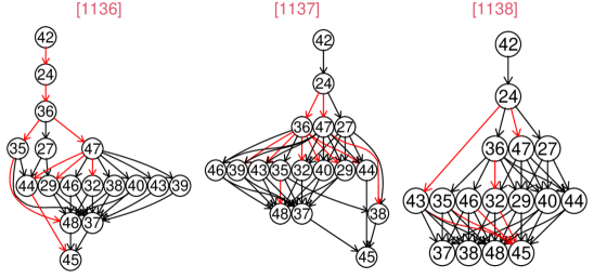
Figure 28: Consensus partial orders for the years 1136-1138 (a selection from the years 1080-1155) under the constrained-effects model of Sec 6.3 but with $K=18$. These transitive reductions should be compared with those in Fig 10. Vertex numbering as Fig 24

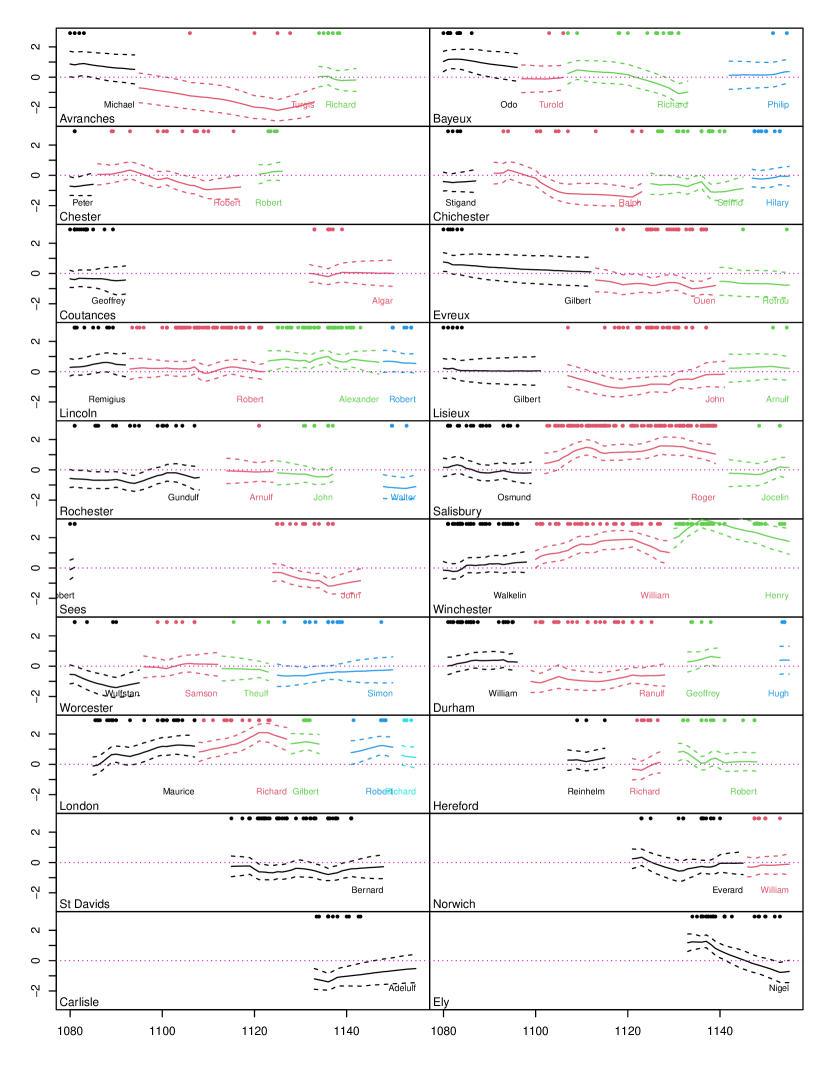
Figure 29: Bishop-authority curves $\bar{U}^{(t)}_{j}$ (solid curves) plotted for each bishop $j\in{\mathcal{M}}$ as a function of time from $b_{j}$ to $e_{j}$ with standard errors at one-sigma in the constrained-effects model of Sec 6.3 but with $K=18$. Compare Fig 11.

Appendix I Parameter estimates from multiple short time-windows

In the partial order models of Secs 6.2, 6.3 and Supp H.3 we assume that $p,\rho,\theta$ do not vary over time. One simple way to check this is to estimate their posterior distributions over short time windows. We use the same intervals (first column of Table 1) as Secs 7.4 and K.2. Results are shown in Fig 30.

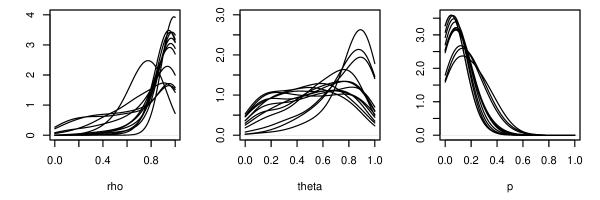
Figure 30: Posterior distributions for $\rho$, $\theta$ and $p$ estimated in each of the twelve time intervals listed in column 1 of Table 1 and discussed in Supp I

The distributions for $\rho$ and $p$ show very little variation over time. The distributions for $\theta$, the degree of correlation between the partial order in one year and the next, do vary somewhat. This density is focused on large values for the first interval 1080-1084 and for intervals after about 1135. The other intervals are close to the (uniform) prior. However, this simply reflects the fact that we get little information about a correlation from a short time interval ($5$ years). We see no evidence here against our assumption that $\rho,\theta$ and $p$ are constant in time.

Appendix J VSP order and Bucket Order analysis - further details

The estimates used to make the plot in Fig 13 are given here. These numbers are discussed in Sec 7.4. The effective sample sizes are for the MCMC output $\mathbb{I}_{h^{(t)}\in{\mathcal{X}}^{(t_{1},t_{2})}}$ where ${\mathcal{X}}$ is $\mathcal{B}$ or ${\mathcal{V}}$ and $h^{(t)}=h(Z(U^{(t)},\beta;s)),\ t=1,...,T$ is taken from a chain targeting $\pi(\rho,\theta,U,\beta,\tau,p|y^{(t_{1},t_{2})})$ using the lists in the time interval $[t_{1},t_{2}]$. These are the samples used to estimate the numerator in Eqn 24. The large ESS values in this table are associated with low posterior probabilities for the events $h\in\mathcal{B}^{(t_{1},t_{2})}$ and $h\in{\mathcal{V}}^{(t_{1},t_{2})}$. The resulting rare event process is approximately iid. It is unclear to us how to measure uncertainty reliably for these cases, but these Bayes factors must be small, as the prior probabilities for the same events are relatively large, and the posterior probabilities are at least much smaller.

Table 1: VSP and Bucket Order Bayes Factors

	Bucket Orders					VSP orders
Period	Prior	Post.	BF	ESS	BF std.err.	Prior	Post.	BF	ESS	BF std.err.
1080-1084	0.085	0	0	-	-	0.22	0	0	-	-
1086-1090	0.15	0.17	1.2	45	0.38	0.31	0.34	1.1	33	0.27
1092-1096	0.27	0.14	0.53	29	0.24	0.48	0.31	0.65	53	0.13
1104-1108	0.18	0.12	0.66	31	0.32	0.36	0.21	0.6	29	0.21
1110-1114	0.42	0.25	0.6	81	0.12	0.72	0.64	0.89	230	0.044
1118-1122	0.1	0.22	2.1	38	0.65	0.24	0.53	2.2	69	0.25
1126-1130	0.16	0.13	0.86	75	0.25	0.32	0.35	1.1	60	0.19
1128-1132	0.084	0.016	0.19	96	0.15	0.22	0.067	0.31	15	0.3
1132-1134	0.088	0.0053	0.06	950	0.027	0.22	0.045	0.21	230	0.063
1138-1142	0.13	0.024	0.18	80	0.13	0.28	0.11	0.37	69	0.13
1144-1148	0.4	0.59	1.5	99	0.12	0.68	0.87	1.3	330	0.027
1150-1154	0.2	0.17	0.83	32	0.32	0.39	0.36	0.93	45	0.19

Appendix K Plackett-Luce models

In the next three sub-Suppwe define and fit two different types of Plackett-Luce model (Luce, 1959; Plackett, 1975). This is done for comparison purposes. In the third sub-Suppwe discuss Luce’s Axiom of choice in relation to our likelihood for lists and relate that to some literature generalising Plackett-Luce.

K.1 Comparison with results from a Plackett-Luce time-series model

Here we specify and fit a time-series Plackett-Luce model like that given in Glickman and Hennessy (2015). Our purpose is to test the conclusions we reached using the partial order model and show that we get similar results when we use a qualitatively different model for the same data. We fit the Plackett-Luce time-series model to the full data from 1080-1155 and compare with results in Secs 6.2 and 6.3. The model is simpler, there is no partial order, but it does share some parameters ($\beta$) and some parameters play very similar roles ($\lambda$ and $U$). Results are remarkably similar. In the next section we will consider formal model comparisons.

K.1.1 Parameters and Likelihood

For $t\in[B,E]$ denote by $\lambda^{(t)}_{j}$ the authority of bishop $j\in{\mathcal{M}}$ in year $t$. Notation for seniority $s$ and seniority effects $\beta$ are unchanged from Sec 2.3.2. The scalar time-series $\lambda_{j}=(\lambda^{(t)}_{j})_{t=B}^{E}$ plays a similar role to the multidimensional time-series of authority variables $U_{j}$ defined in Sec 2.3.3. However, for ease of coding we defined $\lambda^{(t)}_{j}$ for all $t\in[E,B]$ not just $t\in[b_{j},e_{j}]$ as we did for $U_{j}$. This means $\lambda=(\lambda_{j})_{j\in{\mathcal{M}}}$ is a “full” $M\times T$ matrix. Denote by $\lambda^{(t)}=(\lambda^{(t)}_{j})_{j\in{\mathcal{M}}}$ the column vector of $\lambda$-values in each time $t\in[B,E]$.

The times of some of the lists are uncertain so we fixed these to be the centres of their intervals, $\hat{\tau}_{i}=(\tau_{i}^{-}+\tau_{i}^{+})/2$. The Plackett-Luce likelihood is then

$$p_{PL}(y|\lambda,\beta) =\prod_{i=1}^{N}\prod_{j=1}^{n_{i}}\frac{\exp(\lambda^{(\hat{\tau}_{i})}_{y_{ij}}+\beta_{s_{\hat{\tau}_{i},y_{ij}}})}{\sum_{k=j}^{n_{i}}\exp(\lambda^{(\hat{\tau}_{i})}_{y_{ik}}+\beta_{s_{\hat{\tau}_{i},y_{ik}}})}$$ (46)

The “linear predictor” $\lambda^{(t)}_{j}+\beta_{s_{t,j}}$ captures the “status” of bishop $j$ in year $t$ just as the vector $Z^{(t)}_{j}$ did in Sec 2.3.1. The covariates enter in the same way as before (Eqn 11) and so $\lambda^{(t)}_{j}$ is the part of status not determined by seniority. We call this authority to distinguish it from authority $U^{(t)}_{j}$ defined above.

K.1.2 Plackett-Luce Priors

The likelihood in Eqn 46 is invariant under $\lambda\to\lambda+\delta$ and $\beta\to\beta+\delta^{\prime}$ for any $\delta,\delta^{\prime}\in\mathbb{R}$. As noted above in Sec 4.2.1, the $U,\beta$-latent variable model for partial orders has the same feature. We now remove this non-identifiability in our parameterisation.

Consider a projection matrix

$$Q_{M}=I_{M}-\frac{1}{M}\mathbf{1}_{M}\mathbf{1}_{M}^{T},$$

with $I_{M}$ the $M\times M$ identity matrix and $\mathbf{1}_{M}$ a column of $M$ ones. Let $Q_{S_{b}}$ be defined similarly. The matrix $Q_{M}$ projects vectors in $\mathbb{R}^{M}$ to centred vectors $\{v\in\mathbb{R}^{M}:\sum_{j\in{\mathcal{M}}}v_{j}=0_{M}\}$. Under a Plackett-Luce model with covariates for seniority, the generative model for authority is a centred $AR(1)$ process,

$$\lambda^{(t)}=\theta\lambda^{(t-1)}+Q_{M}\epsilon^{(t)},$$

where $\epsilon^{(t)}\sim N(\mathbf{0}_{M},\sigma^{2}I_{M})$ iid for $t=B+1,...,E$. If $\lambda^{(t-1)}$ is centred, then $\lambda^{(t)}$ is also centred. The process is initialised in its prior equilibrium distribution,

$$\lambda^{(B)} =Q_{M}\epsilon^{(b)},$$

where

$$\epsilon^{(b)} \sim N\left(0_{M},\frac{\sigma^{2}}{1-\theta^{2}}I_{M}\right).$$ (47)

Since

$$\lambda^{(t)}_{1}=-\sum_{j=2}^{M}\lambda^{(t)}_{j},\quad\beta_{1}=-\sum_{r=2}^{S}\beta_{r},$$ (48)

we work with a non-singular prior density with parameters $\lambda^{(t)}_{2:M},\ t\in[B,E]$. Denote by $Q_{2:M}$ the $M-1\times M$ matrix obtained by dropping the first row from $Q_{M}$ (with $Q_{2:S_{b}}$ defined similarly). The densities determined by these generative models are

$$\pi(\lambda^{(t)}_{2:M}|\lambda^{(t-1)}_{2:M},\theta,\sigma) =N\left(\lambda^{(t)}_{2:M};\theta\lambda^{(t-1)}_{2:M},\sigma^{2}Q_{2:M}Q_{2:M}^{T}\right),$$

$$\pi(\lambda^{(B)}_{2:M}|\theta,\sigma) =N\left(\lambda^{(B)}_{2:M};\mathbf{0}_{2:M},\frac{\sigma^{2}}{1-\theta^{2}}Q_{2:M}Q_{2:M}^{T}\right),$$

and

$$\pi(\lambda_{2:M}|\theta,\sigma) =\pi(\lambda^{(B)}_{2:M}|\theta,\sigma)\prod_{t=B+1}^{E}\pi(\lambda^{(t)}_{2:M}|\lambda^{(t-1)}_{2:M},\theta,\sigma).$$

The prior on $\beta$ is similarly

$$\pi(\beta)=N(\beta_{2:S_{b}};\mathbf{0}_{S_{b}-1},Q_{2:S_{b}}Q_{2:S_{b}}^{T}).$$ (49)

There is nothing “special” about $\lambda_{1}$ or $\beta_{1}$ in these priors. They are determined by Eqns 48, but they are still exchangeable with the other parameters in the prior. We take a $\mbox{Unif}(0,1)$ prior for $\theta$ and a $\mbox{Gamma}(2,2)$ for $\sigma$ as capturing reasonable variation.

K.1.3 Posterior distribution

The Plackett-Luce posterior is then

$$\pi_{PL}(\lambda_{2:M},\beta_{2:S_{b}},\sigma,\theta|y)\propto p_{PL}(y|\lambda,\beta)\pi(\lambda_{2:M}|\sigma,\theta)\pi(\beta_{2:S_{b}},\sigma,\theta),$$ (50)

with $\lambda_{1}$ and $\beta_{1}$ in $\lambda$ and $\beta$ appearing in $p_{PL}(y|\lambda,\beta)$ given by Eqns 48.

We extended the $\lambda_{j}$-process for each bishop $j\in{\mathcal{M}}$ outside the range $[b_{j},e_{j}]$. This made coding easier, but this means a large set of extra parameters must be brought into equilibrium in the target. However, by the stationarity of an $AR(1)$ process, the posterior marginal (integrating over $\lambda^{(t)}_{j}$ for $t\not\in[b_{j},e_{j}]$) of the fitted model is identical to the model which “starts” the $\lambda_{j}$-process at $t=b_{j}$ with the $AR(1)$ equilibrium in Eqn 47 and terminates it at $t=e_{j}$.

K.1.4 Results for Plackett-Luce Time-series model

We use a simple random-walk MCMC algorithm to target $\pi_{PL}(\lambda_{2:M},\beta_{2:S_{b}},\sigma,\theta|y)$, taking the same data we used in Secs 6.2 and 6.3. We took unconstrained $\beta\in\mathcal{B}_{0}$. Denote by $(\lambda^{(t,l)}_{j},\theta^{(l)},\sigma^{(l)}),\ l=1,...,L$ the realised MCMC samples after thinning and burn-in. The Effective Sample Sizes for the parameters were $\theta(26)$, $\sigma(19)$, $\beta(S_{b}=18\mbox{ parameters, }176-5532)$ $\lambda(4484\mbox{ parameters, }41-1062)$. Mixing for the key parameter vectors $\beta$ and $\lambda$ was fair, and the agreement between results from the two analyses in this section and Secs 6.2 and 6.3 supports our conclusion that the samples are representative.

Results for quantities of historical interest are very similar to those obtained using the partial-order posterior in Eqn 17. The posterior means for $\theta$ and $\sigma$ were $0.93(0.02)$ and $0.69(0.085)$ (posterior standard deviation in parenthesis). The posterior for $\theta$ is similar to its partial order counterpart in Fig 7. Posterior effect $\beta$ distributions are plotted in Fig 8 at right. They are qualitatively the same, and show the same decline with increasing seniority-rank (decreasing seniority) as we saw on the left. In Fig 31 we plot the curves

$$\hat{\lambda}^{(t)}_{j}=\frac{1}{L}\sum_{l=1}^{L}\lambda^{(t,l)}_{j}$$

over $t\in[b_{j},e_{j}]$ for each $j$ arranged by diocese as we did for $\bar{U}^{(t)}_{j}$ defined in Sec 4.2.1. The resulting authority-measures show similar dependence on time. This shows that our results for these features are robust.

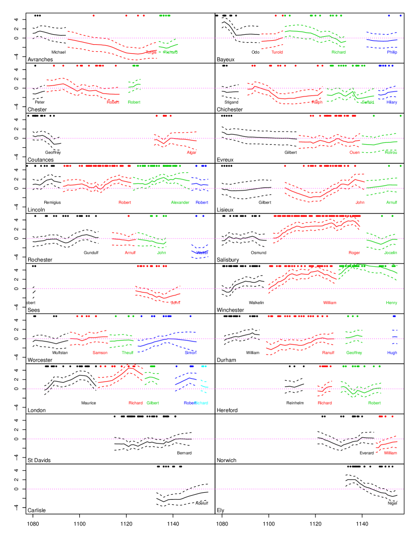
Figure 31: Authority-curves $\hat{\lambda}^{(t)}_{j}$ over $t\in[b_{j},e_{j}]$ for each $j\in{\mathcal{M}}$ arranged by diocese, for the Plackett-Luce time-series model in Supp K.1. See Fig 11 for details and comparison.

K.2 Comparison with a Plackett-Luce mixture model

K.2.1 Parameters and Model

In this section we define a Plackett-Luce mixture model for list data taken from an interval of time $[t_{1},t_{2}]$ which is short enough to allow us to drop time dependence and covariates. The Leave-One-Out cross validation we use below is time consuming and we do this for ease of computation. We fit this model and a partial order model without covariates and carry out model comparison between the two models. Dropping time-varying covariates is natural when working in a short time window, as the effects due to bishop and seniority cannot be separated. Denote by ${\mathcal{I}}_{t_{1},t_{2}}$ the indices of the list data covered by the window (at least half of the years $[\tau_{i}^{-},\tau_{i}^{+}]$ fall within $[t_{1},t_{2}]$) and let $N_{t_{1},t_{2}}=|{\mathcal{I}}_{t_{1},t_{2}}|$ be the number of lists in this window. Let $y^{(t_{1},t_{2})}=(y_{i})_{i\in{\mathcal{I}}_{t_{1},t_{2}}}$ be the windowed data. A finite mixture of Plackett-Luce models was proposed as a robust model for ranked data with incomplete lists (“partially ranked data”, Mollica and Tardella (2017, 2020). A mixture of $D$ Plackett-Luce models for ranking a set ${\mathcal{M}}_{t_{1},t_{2}}=\cup_{t\in[t_{1},t_{2}]}{\mathcal{M}}_{t}$ containing $m_{t_{1},t_{2}}=|{\mathcal{M}}_{t_{1},t_{2}}|$ actors assumes that lists are sampled from a heterogeneous population composed of $D$ sub-populations. Each sub-population is modeled by one of the mixture components with Plackett-Luce status vector $\lambda^{(d)}\in\mathbb{R}^{m_{t_{1},t_{2}}},\ d\in[D]$. Let $\lambda=(\lambda^{(d)})_{d\in[D]}$ be the $m_{t_{1},t_{2}}\times D$ matrix of status parameters.

The likelihood for a mixture of $D$ Plackett-Luce models is then

$$p_{mix\,PL}(y^{(t_{1},t_{2})}|\lambda,\omega)=\prod_{i\in{\mathcal{I}}_{t_{1},t_{2}}}\sum_{d=1}^{D}\omega_{d}\prod_{j=1}^{n_{i}}\frac{\exp(\lambda^{(d)}_{y_{i,j}})}{\sum_{k=j}^{n_{i}}\exp(\lambda^{(d)}_{y_{i,k}})},$$ (51)

where $\omega_{1},...,\omega_{D}$ are weights of mixture components and $\sum_{d=1}^{D}\omega_{d}=1$. Noninformative priors suggested by Mollica and Tardella (2020) are assigned with $\exp(\lambda^{(d)}_{j})\sim\mbox{Gamma}(1,0,001)$ for $j\in{\mathcal{M}}_{t_{1},t_{2}}$ and $\omega_{1},...,\omega_{D}\sim Dir(1,...,1)$.

The posterior is

$$\pi_{mix\,PL}(\lambda,\omega)\propto\pi(\lambda,\omega)p_{mix\,PL}(y^{(t_{1},t_{2})}|\lambda,\omega).$$

We used the MCMC sampler available the R-package PLMIX provided by Mollica and Tardella (2020) to target $\pi_{mix\,PL}$. This sampler uses a data augmentation scheme due to Caron and Doucet (2012).

In order to fit the model we must select the number of mixture components $D$. This is related to Bayesian model comparison. The PLMIX offers several model selection criteria to choose the number of mixture components. We used the Deviation Information Criterion. The selected $D$-values are given in the third column of Table 2.

K.2.2 Model comparison

The expected log pointwise predictive density (ELPD, Vehtari et al. (2017)) measures the posterior predictive accuracy of a model. It is relatively straightforward to estimate and one natural measure of goodness of fit. Let $Y\in\mathcal{P}_{O}$ be a single generic list with membership $O\subseteq{\mathcal{M}}_{t_{1},t_{2}}$. Suppose the true generative model for a list is $Y\sim f_{O}$. Denote by $p_{A,O}(Y|y_{y_{1},y_{2}})$ the posterior predictive probability for $Y$ in model $A$ when the membership of list $Y$ is $O$. The ELPD for model $A\in\{\mbox{Plackett-Luce, Partial order}\}$ conditioned on the observed data is

$$\mbox{elpd}(A|y^{(t_{1},t_{2})}) =\sum^{m_{t_{1},t_{2}}}_{i=1}E_{Y\sim f_{o_{i}}}(\log p_{A,o_{i}}(Y|y^{(t_{1},t_{2})})),$$

$$=\sum^{m_{t_{1},t_{2}}}_{i=1}\left[\sum_{Y\in\mathcal{P}_{o_{i}}}f_{o_{i}}(Y)\,\log p_{A,o_{i}}(Y|y^{(t_{1},t_{2})})\right]\,.$$

The expectation is (up to a constant) the negative of the KL divergence between the true generative model for a list with membership $o_{i}$ and the model-$A$ posterior predictive for that list. We favour models with larger values of the elpd.

We do not know $f_{O}$ but we do know the data are sampled from this distribution, so we follow Vehtari et al. (2017) and use leave one-out cross validation (LOO-CV) to estimate $\mbox{elpd}(A|y^{(t_{1},t_{2})})$. Our estimator is

$$\widehat{\mbox{elpd}}(A|y^{(t_{1},t_{2})})=\sum^{m_{t_{1},t_{2}}}_{i=1}\log p(y_{i}|y^{(t_{1},t_{2})}_{(-i)})$$ (52)

where $y^{(t_{1},t_{2})}_{(-i)}=y^{(t_{1},t_{2})}\setminus\{y_{i}\}$ so the $i$-th observation is left out.

K.2.3 Test results

Table 2: ELPD estimates and standard errors for twelve periods.

Period	$\#$ lists	Plackett-Luce Mixture		Partial-order
$[t_{1},t_{2}]$	$m_{[t_{1},t_{2}]}$	components $D$	$\widehat{\mbox{elpd}}$	$\widehat{\mbox{elpd}}$
1080-1084	26	2	-162.52 (17.55)	-54.35 (11.80)
1086-1090	10	1	-61.43 (14.43)	-23.33 (6.26)
1092-1096	13	1	-49.46 (8.55)	-23.03 (7.98)
1104-1108	23	1	-95.56 (10.15)	-41.08 (9.69)
1110-1114	21	1	-59.93 (8.16)	-33.55 (9.62)
1118-1122	20	2	-89.01 (12.36)	-21.07 (6.99)
1126-1130	25	2	-113.03 (11.77)	-36.13 (9.21)
1128-1132	33	2	-190.34 (16.37)	-73.97 (13.30)
1132-1134	19	2	-110.49 (22.07)	-35.66 (9.91)
1138-1142	32	1	-186.09 (16.77)	-88.09 (25.58)
1144-1148	7	1	-42.15 (4.26)	-17.56 (8.33)
1150-1154	11	1	-60.05 (11.27)	-16.53 (4.20)

In Table 2 the twelve short periods $[t_{1},t_{2}]$ we chose are given in the first column. The same periods are used to for numerical comparison with VSP and Bucket Orders in Table 1. The number of lists $m_{t_{1},t_{2}}$ covered by each interval is in the second column. We estimate the posterior predictive probability for each omitted list in a period by averaging its likelihood over posterior samples, so the number of MCMC runs for each entry in columns four and five is equal to $m_{t_{1},t_{2}}$. This impacted our choices for the locations of time intervals as we had to avoid periods with too few lists or too many long lists.

The elpd’s in column five are uniformly larger than those in column four, so the partial order model is clearly favoured over the Plackett-Luce mixture model for all these short periods. This may be because the partial order is able to restrict the set of probable lists more tightly around the lists in the data, while the fitted Plackett-Luce mixture is relatively more dispersed over lists. The reported uncertainty estimate is just the sample variation of the mean of the $m_{t_{1},t_{2}}$-samples used to form the estimate. It is likely to be an underestimate because the same lists appear in test and training positions in different terms in the sum, so its terms are correlated (Bengio and Grandvalet, 2004; Sivula et al., 2022).

K.3 The choice axiom of Luce

It may be shown that the class of Plackett-Luce models (Plackett, 1975; Luce, 1959) for random rank-order lists $Y$ are determined by a small set of axioms restricting the distribution of random lists. See Luce (1977) for an overview. The axioms view the lists as generated by a sequence of “repeated selections” (Seshadri et al., 2020). The first axiom (independence from irrelevant alternatives) would in our setting require that, if $Y\in\mathcal{P}_{[M]}$ is a random list on all actors and $\tilde{Y}\in\mathcal{P}_{O}$ is a random list on a subset $O\subset[M]$ then for $j\in O$ and $H\in{\mathcal{H}}_{[M]}$, we must have $\Pr(\tilde{Y}_{1}=j|H[O])=P(Y_{1}=j|H,Y_{1}\in O)$. This axiom is satisfied by the Placket Luce model but is not satisfied by the model in Eqn 3, or any of the partial-order-based observations models we give below. For example, the partial order $H=\{\langle 2,3\rangle\}$ on the ground set $[M]=\{1,2,3\}$ has three linear extensions $\mathcal{L}[H]=\{(1,2,3),(2,1,3),(2,3,1)\}$ so if $Y\sim\mbox{Unif}(\mathcal{L}[H])$ and $O=\{1,2\}$ then $P(Y_{1}=1|H,j\in O)=1/3$. However, $H[O]=\emptyset$ and $\mathcal{L}[\emptyset]=\{(1,2),(2,1)\}$ so if $\tilde{Y}\sim\mbox{Unif}(\mathcal{L}[H[O]])$ then $\Pr(\tilde{Y}_{1}=j|H[O])=1/2$. Plackett-Luce models are discussed further in Supp K.1 and K.2.

Ragain and Ugander (2018) and Seshadri et al. (2020) define and analyse a large class of Contextual Repeated Selection (CRS) models which include Plackett-Luce and many other well-known ranking models as special cases. We will see (in Eqn 4 below) that we can think of the lists in our observation models as being generated by repeated selection of the top element. The CRS model does not have the same physical representation to a hierarchy relation in a PO and, does not encode transitivity. i.e., $a\succ b\succ c$ is not recovered by the CRS given linear extensions for $a\succ b$ and $b\succ c$.

Appendix L Checks on synthetic data

L.1 Checks on synthetic data: replicate main analysis

We simulated synthetic data with the same structure as the real data and checked we could recover true parameter values. We took true values of $\rho,\theta,\beta,U,\tau,p$ sampled from the posterior in Sec 6.2 (the last sampled state in the run in Fig 22) and simulated data $y^{\prime}_{i}\sim p_{(U)}(\cdot|h^{(\tau_{i})}[o_{i}],p),\ i\in{\mathcal{I}}$.

MCMC output targeting the posterior for the synthetic data $y^{\prime}$ is shown in Fig 32. The true $\rho,\theta$ and $p$ values fall within the support of their respective posteriors in Fig 33. The reconstructions agree well and in particular the credible intervals for $\bar{Z}$ in Fig 35 and $\beta$ in Fig 34 cover the truth well.

In order to check partial order reconstruction in the fitted consensus orders we report false positive and negative relation-counts in Fig 36. These are computed using the consensus partial order $\bar{h}^{(t)}(\xi)=(E_{t}(\xi),{\mathcal{M}}_{t}),\ t\in[B,E]$ defined in Eqn 29. If $H^{(t)}$ is the set of order relations (ie edges) in the true partial order in year $t$ then the false negative count in year $t$ is $|H^{(t)}\setminus E_{t}(\xi)|$, false positive is $|E_{t}(\xi)\setminus H^{(t)}|$, true positive $|H^{(t)}\cap E_{t}(\xi)|$ and so on. True negatives (blue) and true positives (in green) dominate in the later years and false negatives (black) are low, though there are many false positives (red) in the period up to 1110. This suggests that many of the black edges (with support at the low level of $\xi=0.5$) in the consensus partial orders in for example Fig 23 will be false positives. However, the red edges with support at $\xi=0.9$ will have far fewer false positives.

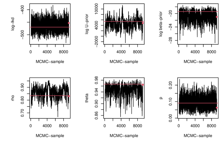
Figure 32: Synthetic Data. Selected MCMC traces from the unconstrained seniority-effect analysis in Supp L.1. Horizontal red lines show values at truth.

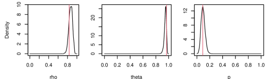
Figure 33: Synthetic Data. Posterior parameter densities for $\rho,\theta$ and $p$ from the unconstrained seniority effects analysis in Supp L.1. Vertical red lines show true values.

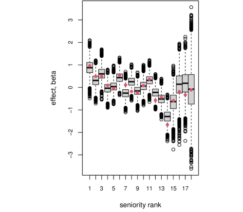
Figure 34: Synthetic Data. Marginal posterior distributions of seniority effect parameters from the unconstrained seniority effects analysis in Supp L.1. Red dots show true values.

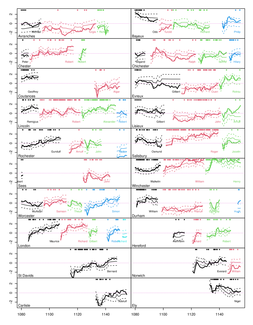
Figure 35: Synthetic Data. Bishop-status curves $\hat{Z}^{(t)}_{j}$ (thin solid curves) plotted for each bishop $j\in{\mathcal{M}}$ as a function of time from $b_{j}$ to $e_{j}$ with standard errors at one-sigma. The dots along the top of each graph show the times of the lists in which the color-matched bishop below appeared. This is output from the constrained seniority effects analysis in Sec L.1. The thick solid lines show the true values.

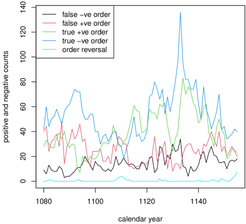
Figure 36: Synthetic Data. False positive and negative counts for from the unconstrained seniority effects analysis in Supp L.1. The classification threshold for edge $\langle j_{1},j_{2}\rangle$ to be present was set at $\hat{\xi}_{\langle j_{1},j_{2}\rangle}\geq 0.5$ (equivalent to predicting the consensus partial order including red and black edges).

L.2 Checks on synthetic data: when the true orders are total orders

In some feedback from historians a concern was expressed that the relatively shallow partial orders we see reflect differences in how often bishops witness and that the “true” orders were deeper. We tested this by simulating synthetic data in which the true partial orders all had depth close to or equal the maximum $m_{t}$ in each year $t\in[B,E]$, but using the same list memberships $o_{i},\ i\in{\mathcal{I}}$ as the real data.

We set the “true” noise at level $p^{*}=0.1$ typical of that seen in our fit. We used the same time intervals for the lists as in the real data so the synthetic data has the same structure as the real data, but different list orders. We simulated a “true sequence” $h^{*}={h^{*}}^{(t)},\ t\in[B,E]$ of high-depth orders (by setting $\rho^{*}=0.99999$ close to one) and true observation times $\tau^{*}$ from the prior, then simulated synthetic-data lists according to the observation model $y^{\prime}_{i}\sim p_{(U)}(\cdot|{h^{*}}^{(\tau^{*}_{i})}[o_{i}],p^{*}),\ i\in{\mathcal{I}}$. We then simulated the posterior $\pi(\rho,\theta,U,\beta,\tau,p|y^{\prime})$ and checked consensus partial orders and checked we recovered the true depth. The posterior depth distribution is shown in Fig 37 at right. The posterior shows good overlap with the truth despite it being on the boundary of the space.

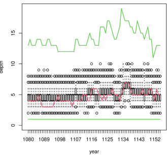
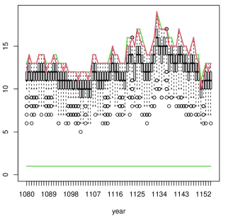
Figure 37: Synthetic data taking the true order sequence $h^{*}$ to be a sample from the Sec 6.3-posterior (left) or a sequence of deep orders sampled from the prior (right). Fitting with prior settings as Sec 6.3 shows good overlap between truth and posterior. This suggests the prior is not biasing. The grean lines show the minimum and maximum possible partial order depth in each year and the red line shows the depth of the true partial order used to generate the synthetic data.

In summary, we reconstructed the true total orders well with good depth. If the true orders were total orders we would see this in our analysis. We do not, so we conclude that the uneven list memberships, dates and list-lengths are not obscuring some hidden deeper order.

It is of interest to consider what happens when the true partial order has depth 1, so the partial order is the empty order and there are no constraints at all. The data $y_{i}$ would then all be uniform random permutations of the list membership vectors $o_{i},\ i\in{\mathcal{I}}$ and there is then a non-identifiability. The model can fit uniform random permutations by making $p\simeq 1$, so taking high noise, and any partial order we like (as we get back uniform random permutations as $p\to 1$ irrespective of the underlying partial order) or by making the partial order empty (so depth 1) and letting $p$ be any value. In some experiments which we do not report on synthetic data with depth 1 we found that the model favoured the $p\to 1$ fit (as the prior weights against depth 1). Again, the fit for our data favours small noise, $p\simeq 0.1$ so by the same reasoning as for total orders, this non-identifiability is not an issue for the data we actually have. This has been called the “principle of sufficient reason”: the prior is well behaved over the range of parameter values actually supported by the data.

Appendix M Fixed-time model

A simpler version of the model summarised in Sec 2.4 outlined in Nicholls and Muir Watt (2011), without any time series structure, may be of interest so we give the simplest model of this sort. Covariates depending on time (and their effects $\beta$) have been dropped. They might be replaced with covariates which vary across lists. However we do not pursue this.

In this fixed-time setting we have $N$ lists with labels $i\in{\mathcal{I}}$, $M$ bishops with labels $j\in{\mathcal{M}}$, $Z$ is an $M\times K$ feature matrix (not a time series of matrices) with rows $Z_{j}\in\mathbb{R}^{K}$ giving the $K$ status features for each bishop, and $H=h(Z)$ is a partial order on $[M]$. All the lists have the same equal time, so $\tau$ is dropped. The generative model is

$$\rho \sim\mbox{Beta}(1,\gamma)$$

$$Z_{j} \sim N(0,\Sigma^{(\rho)}),\ \mbox{iid for}\ j\in{\mathcal{M}}$$

$$p \sim\mbox{Beta}(1,\delta),$$

then $$H=h(Z)$$ using Eqn 10 and the data are realised

$$y_{i} \sim p(\cdot|H[o_{i}],p),\quad\mbox{independently for $i\in{\mathcal{I}}$}.$$

The joint posterior distribution is

$$\pi(\rho,Z,p|y)\propto\pi(\rho,p)\prod_{j\in{\mathcal{M}}}N(Z_{j};0,\Sigma^{(\rho)})\prod_{i=1}^{N}p(y_{i}|H[o_{i}],p)\,.$$ (69)

References

- Arcagni et al. (2022) Arcagni, A., A. Avellone, and M. Fattore (2022). Complexity reduction and approximation of multidomain systems of partially ordered data. Computational Statistics & Data Analysis 173, 107520.
- Asfaw et al. (2017) Asfaw, D., V. Vitelli, Ø. Sørensen, E. Arjas, and A. Frigessi (2017). Time-varying rankings with the Bayesian Mallows model. Stat 6(1), 14–30.
- Bates (1998) Bates, D. (1998). The Acta of William I, 1066–1087. Regesta regum Anglo-Normannorum 1066-1154. Oxford.
- Bates (2013) Bates, D. (2013). The Normans and Empire. Ford lectures. OUP Oxford.
- Beerenwinkel et al. (2007) Beerenwinkel, N., N. Eriksson, and B. Sturmfels (2007). Conjunctive bayesian networks. Bernoulli 13(4), 893–909.
- Bengio and Grandvalet (2004) Bengio, Y. and Y. Grandvalet (2004). No unbiased estimator of the variance of k-fold cross-validation. Journal of Machine Learning Research 5, 1089–1105.
- Bogart (1973) Bogart, K. P. (1973, 5). Maximal dimensional partially ordered sets I. Hiraguchi’s theorem. Discrete Mathematics 5, 21–31.
- Brightwell (1993) Brightwell, G. (1993). Surveys in Combinatorics, Volume 187 of London Mathematical Society Lecture Note Series, Chapter Models of random partial orders, pp. 53–83. Cambridge Univeristy Press.
- Brightwell and Winkler (1991) Brightwell, G. and P. Winkler (1991). Counting linear extensions. Order 8(3), 225–242.
- Caron and Doucet (2012) Caron, F. and A. Doucet (2012). Efficient Bayesian inference for generalized Bradley-Terry models. J. Comput. Graph. Statist. 21(1), 174–196.
- Clover and Gibson (1979) Clover, H. and M. Gibson (1979). The Letters of Lanfranc, Archbishop of Canterbury. Oxford.
- Cronne and Davis (1968) Cronne, H. A. and R. H. C. Davis (1968). Regesta Regis Stephani ac Mathildis Imperatricis ac Gaufridi et Henrici Ducum Normannorum, 1135–1154. Regesta regum Anglo-Normannorum 1066-1154. Oxford.
- Davis and Whitwell (1913) Davis, H. and R. Whitwell (1913). Regesta regum Anglo-Normannorum 1066-1154: Regesta Willelmi Conquestoris et Willelmi Rufi 1066-1100. Regesta regum Anglo-Normannorum 1066-1154. Oxford.
- Dushnik and Miller (1941) Dushnik, B. and E. W. Miller (1941). Partially ordered sets. American Journal of Mathematics 63(3), 600–610.
- FEA (2022) FEA (2022). Fasti Ecclesiae Anglicanae, 1066-1300. London: Institute of Historical Research; British History Online; Last accessed 22 October 2022; http://www.british-history.ac.uk/fasti-ecclesiae/.
- Froehlich et al. (2007) Froehlich, H., M. Fellmann, H. Sueltmann, A. Poustka, and T. Beissbarth (2007). Large scale statistical inference of signaling pathways from RNAi and microarray data. BMC Bioinformatics 8(386).
- Gionis et al. (2006) Gionis, A., H. Mannila, K. Puolamäki, and A. Ukkonen (2006). Algorithms for discovering bucket orders from data. In Proceedings of the 12th ACM SIGKDD international conference on Knowledge discovery and data mining, pp. 561–566.
- Glickman and Hennessy (2015) Glickman, M. E. and J. Hennessy (2015). A stochastic rank ordered logit model for rating multi-competitor games and sports. Journal of Quantitative Analysis in Sports 11(3), 131–144.
- Hiraguchi (1951) Hiraguchi, T. (1951). On the dimension of partially ordered sets. The science reports of the Kanazawa University 1, 77–94.
- Jagabathula et al. (2022) Jagabathula, S., D. Mitrofanov, and G. Vulcano (2022). Personalized retail promotions through a directed acyclic graph–based representation of customer preferences. Operations Research 70(2), 641–665.
- Jagabathula and Vulcano (2017) Jagabathula, S. and G. Vulcano (2017). A Partial-Order-based model to estimate individual preferences using panel data. Management Science 64(4), 1609–1628.
- Jiang et al. (2023) Jiang, C., G. K. Nicholls, and J. E. Lee (2023). Bayesian inference for vertex-series-parallel partial orders. In Proceedings of the Thirty-Ninth Conference on Uncertainty in Artificial Intelligence. (To appear).
- Johnson and Cronne (1966) Johnson, C. and H. A. Cronne (1966). Regesta Henrici Primi : 1100-1135. Regesta regum Anglo-Normannorum 1066-1154. Oxford.
- Johnson (2013) Johnson, D. (2013, 10). Bishops and deans: London and the province of Canterbury in the twelfth century*. Historical Research 86(234), 551–578.
- Kangas et al. (2016) Kangas, K., T. Hankala, T. Niinimäki, and M. Koivisto (2016). Counting linear extensions of sparse posets. In Proceedings of the Twenty-Fifth International Joint Conference on Artificial Intelligence, IJCAI’16, pp. 603–609. AAAI Press.
- Kangas et al. (2019) Kangas, K., M. Koivisto, and S. Salonen (2019). A faster tree-decomposition based algorithm for counting linear extensions. Algorithmica, 1–18.
- Karzanov and Khachiyan (1991) Karzanov, A. and L. Khachiyan (1991). On the conductance of order Markov chains. Order 8, 7–15.
- Kleitman and Rothschild (1975) Kleitman, D. J. and B. L. Rothschild (1975). Asymptotic enumeration of partial orders on a finite set. Transactions of the American Mathematical Society 205, 205–220.
- Knuth and Szwarcfiter (1974) Knuth, D. E. and J. L. Szwarcfiter (1974). A structured program to generate all topological sorting arrangements. Information Processing Letters 2(6), 153–157.
- Liu et al. (2019) Liu, A., Z. Zhao, C. Liao, P. Lu, and L. Xia (2019). Learning Plackett-Luce mixtures from partial preferences. In Proceedings of the AAAI Conference on Artificial Intelligence, Volume 33, pp. 4328–4335.
- Luce (1977) Luce, R. (1977). The choice axiom after twenty years. Journal of Mathematical Psychology 15(3), 215–233.
- Luce (1959) Luce, R. D. (1959). On the possible psychophysical laws. Psychological review 66(2), 81.
- Mallows (1957) Mallows, C. L. (1957). Non-null ranking models. i. Biometrika 44(1/2), 114–130.
- Mannila (2008) Mannila, H. (2008). Finding total and partial orders from data for seriation. In J.-F. Boucault (Ed.), Discovery Science, Volume 5255 of LNAI, Berlin Heidelberg, pp. 16–25. Springer-Verlag.
- Mannila and Meek (2000) Mannila, H. and C. Meek (2000). Global partial orders from sequential data. In Proceedings of the Sixth ACM SIGKDD International Conference on Knowledge Discovery and Data Mining, KDD ’00, New York, NY, USA, pp. 161–168. Association for Computing Machinery.
- Meilă and Chen (2010) Meilă, M. and H. Chen (2010). Dirichlet process mixtures of generalized Mallows models. In Proceedings of the Twenty-Sixth Conference on Uncertainty in Artificial Intelligence, UAI’10, Arlington, Virginia, USA, pp. 358–367. AUAI Press.
- Mogapi (2009) Mogapi, O. (2009). A Latent Partial Order Model for Social Networks. Ph. D. thesis, University of Oxford.
- Mollica and Tardella (2017) Mollica, C. and L. Tardella (2017). Bayesian Plackett-Luce mixture models for partially ranked data. Psychometrika 82(2), 442–458.
- Mollica and Tardella (2020) Mollica, C. and L. Tardella (2020). PLMIX: an R package for modelling and clustering partially ranked data. Journal of Statistical Computation and Simulation 90(5), 925–959.
- Muir Watt (2015) Muir Watt, A. (2015). Inference for partial orders from random linear extensions. Ph. D. thesis, University of Oxford.
- Nicholls and Muir Watt (2011) Nicholls, G. K. and A. Muir Watt (2011). Partial order models for episcopal social status in 12th century England. IWSM 2011, 437.
- Niinimäki et al. (2016) Niinimäki, T., P. Parviainen, and M. Koivisto (2016). Structure discovery in Bayesian networks by sampling partial orders. Journal of Machine Learning Research 17(57), 1–47.
- OEIS Foundation Inc (2022) OEIS Foundation Inc, . (2022). The on-line encyclopedia of integer sequences. Published electronically at https://oeis.org.
- Peyhardi et al. (2016) Peyhardi, J., C. Trottier, and Y. Guédon (2016). Partitioned conditional generalized linear models for categorical responses. Statistical Modelling 16(4), 297–321.
- Plackett (1975) Plackett, R. L. (1975). The analysis of permutations. Journal of the Royal Statistical Society: Series C (Applied Statistics) 24(2), 193–202.