Reliability Study of Battery Lives: A Functional Degradation Analysis Approach

Abstract

Renewable energy is critical for combating climate change, whose first step is the storage of electricity generated from renewable energy sources. Li-ion batteries are a popular kind of storage units. Their continuous usage through charge-discharge cycles eventually leads to degradation. This can be visualized in plotting voltage discharge curves (VDCs) over discharge cycles. Studies of battery degradation have mostly concentrated on modeling degradation through one scalar measurement summarizing each VDC. Such simplification of curves can lead to inaccurate predictive models. Here we analyze the degradation of rechargeable Li-ion batteries from a NASA data set through modeling and predicting their full VDCs. With techniques from longitudinal and functional data analysis, we propose a new two-step predictive modeling procedure for functional responses residing on heterogeneous domains. We first predict the shapes and domain end points of VDCs using functional regression models. Then we integrate these predictions to perform a degradation analysis. Our approach is fully functional, allows the incorporation of usage information, produces predictions in a curve form, and thus provides flexibility in the assessment of battery degradation. Through extensive simulation studies and cross-validated data analysis, our approach demonstrates better prediction than the existing approach of modeling degradation directly with aggregated data.

Key Words: degradation analysis, functional data analysis, longitudinal data, rechargeable batteries.

1 Introduction

Renewable energy plays an important role in global energy security and global warming control olabi2022renewable. Commonly used renewable energy technologies include solar power technology, wind turbines, biomass technology for power generation and tidal energy technologies (bull2001renewable and panwar2011role). Once electricity is generated from those renewable energy technologies, energy storage batteries are needed for energy to be stored when available and released when needed. Li-ion batteries are widely used for energy storage and one significant application is on electric vehicles (diouf2015potential and castelvecchi2021electric).

An important issue in these applications is the assessment of battery life under a certain use condition. Accurate assessment of battery lives is critical for large-scale deployments of renewable technology. This motivates battery life studies like the one reported in saha2007battery, where the question of interest is how many charge-discharge cycles a battery can sustain before it reaches a failure threshold in terms of capacity loss.

Even though there is vast literature on the modeling and prediction of Li-ion battery lives, existing analyses are mostly straightforward applications of traditional statistical methods from a simplistic view of the data. For example, existing studies do not take full advantage of the whole discharge curves, whereas each curve gives much more details, than a simple summary number such as the area under the curve, on how the battery performed in a cycle. Figure 1 illustrates the available voltage discharge curves (VDCs) of two batteries in the data set of interest. An aggregation summary such as area under the curve does represent a type of degradation measure, but there is clearly the risk of information loss since the whole curve is not taken into account. This motivates us to adopt the functional data analysis (FDA) approach to model and predict battery lives. Under the FDA framework, each curve is viewed as a functional observation and we shall model the VDCs directly through functional mixed-effects models. Ever since its introduction by the seminal monograph fda1997, FDA has found many extensions to various areas in statistics; see, e.g., the recent reviews in Wang2016, recentdev2019, and fda_jmva. To the best of our knowledge, our work is the first FDA approach in the area of battery life modeling and more generally, in the area of degradation modeling too.

Modeling functional curves with covariate information falls under the umbrella of functional response models. Existing functional response models require a common domain for the functional responses. However, in our battery data, each VDC has its distinctive domain, ranging from the start of the discharge cycle to the so-called end of discharge (EOD) time saha2009pf. Therefore, we first introduce a scaled version of VDCs where each VDC is scaled by its EOD to lie on the common domain of $[0,1]$. Then we consider a model consisting of two parts. One part models the EODs and the other models the scaled VDCs. For the predictors in the models, experimental conditions are the natural covariates to include. The cycle number is also necessary for the modeling of the degradation patterns. Some other covariates in consideration include the resting time between cycles, the EOD of the previous cycle, and the scaled VDC itself. To model the scaled VDCs, we first conduct a functional principal component analysis to represent each curve by its projected scores onto the leading functional principal components. Then a multivariate mixed-effects model is fitted with the random effects introduced to incorporate the within-battery correlations between VDCs. For the EODs, we consider two version of mixed-effects models, with or without the inclusion of the functional covariate of scaled VDC. Our degradation analyses, with three versions, are all based on these functional models of the scaled curves and EODs. The first version is the standard general path model where degradation amounts computed from fitted VDCs at the observed cycles (or training cycles) are the only inputs to fit the prediction model for degradation amounts. The other two versions, corresponding to the two versions of EOD models, would use the functional models to predict scaled VDCs and EODs first and then use them to calculate the predicted degradation amounts.

Through extensive simulations and comprehensive analysis of the battery data, we show the great potential of a fully FDA approach to degradation analysis of batteries. In particular, it has the following advantages against the standard or existing approaches: (i) the framework allows an easy incorporation of covariates such as experimental conditions, which are critical factors for battery degradation but have been largely ignored by the existing literature; (ii) it makes full use of the whole VDCs, ensuring a minimal loss of information from the original data; (iii) it is demonstrated in our numerical studies to have much better prediction performance than the traditional aggregation methods, which is essential in degradation analysis; and (iv) its predictions include the predictions for the EODs and scaled VDCs, which can be assembled to obtain a prediction for the original VDC at a future cycle.

The rest of the paper is as follows. In Section 2, we introduce the NASA battery dataset for the analysis. We give an overview of the existing literature studying this dataset under battery degradation and health monitoring framework. We discuss insights we gain from these work as well as their gaps in modeling VDCs that inspire this work. In Section 3, we present the methodology in details including notations, modeling, predicting and degradation analysis. In Section 4, we conduct a simulation study to test the performance of our proposed method against a standard method when we hold the truth about the data generation mechanism. In Section 5, we present the real data analysis using the developed framework. Finally, we conclude with some summaries and areas for future research in Section 6.

2 Battery Life Study from NASA Ames Prognostics Data Repository

The study we consider here is from the NASA Prognostics Data Repository [Saha and GoebelSaha and Goebel2007]. In the study, Li-ion batteries were tested through cycles of charge and discharge at different room temperature and conditions. Experimenters performed the same charging procedure for all batteries after each discharge cycle. The lifetime measure for batteries was the number of discharge cycles. The experimental conditions for discharge cycles varied among batteries. We focus on the following conditions.

• Testing temperature (temp): room temperature ($24^{\circ}\text{C}$), elevated temperature ($43^{\circ}\text{C}$), or low temperature ($4^{\circ}\text{C}$).

• Discharge current (dc): 1 Amp, 2 Amps, or 4 Amps.

• Level of voltage where discharge ends or stopping voltage (sv): 2 Volts, 2.2 Volts, 2.5 Volts, or 2.7 Volts.

The data were collected from 20 batteries with constant experimental conditions across discharge cycles in the experiment. Throughout the discharge cycles of each battery, measurements of discharge voltage levels were recorded. As shown in Figure 1 for two batteries, the VDCs for each battery clearly show a degrading pattern. In early discharge cycles, the battery voltage stays high for a longer time until a sharp drop at a later time in the cycle. As the cycle number increases, the battery voltage sustains for a shorter time and drops sharply at an earlier time in the cycle. This pattern is revealed by the motion of the discharge curves moving inward in Figure 1.

Figure 1: Voltage discharge curves by cycles number for battery B0005 (discharge current: 2 Amps, Stopping voltage: 2.7 Volts, temperature: $24^{\circ}$C) and battery B0030 (discharge current: 4 Amps, Stopping voltage: 2.2 Volts, temperature: $43^{\circ}$C).

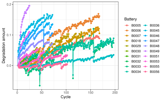
Figure 2: Degradation amount by cycle number and battery determined by $L^{1}$-norm of batteries’ voltage discharge curves.

This is a well-known dataset in the literature of battery health prognostics. The main focus of health prognostics is on studying the state of health (SOH) of batteries with the goal of predicting the remaining useful life (RUL). The RUL is determined by how close a battery’s capacity is to a preset threshold. As a standard measurement, the battery capacity at a cycle is closely related to the area under the corresponding VDC. Therefore, most existing methods have focused on direct modeling and predicting battery capacity along discharge cycles on the degradation path.

Among the earliest work, saha2009pf proposed to predict battery capacity under the particle filtering (PF) framework. They also developed a Rao-Blackwellized PF approach in saha2008rbpf to reduce uncertainty on capacity prediction. A comparison of their methods is available in saha2009comparison. Since then various statistical and machine learning methods have been proposed for the battery capacity prediction problem. Examples of statistical models include stochastic models using autoregressive processes liu2012nlar or Wiener processes (tang2014weiner, shen2018wiener), and Gaussian process regression (liu2012gpr, liu2013gpfr, he2015gpr, richardson2017gpr, tagade2020deep). Examples of machine learning techniques include naïve Bayes ng2014naive, support vector machine patil2015svm, relevance vector machine liu2015rvm, genetic algorithms yu2022ega, and neural networks (sbarufatti2017rbnn, nascimento2021hybrid). liu2014fusion provided a fusion method integrating regularized particle filtering and autoregressive models. A comprehensive review of these methods can be found in martin2022comparison.

However, none of the aforementioned work included all the 20 batteries in their analyses. Most work focuses only on the first four batteries (B0005, B0006, B0007, and B0018). These batteries shared the same experimental conditions of temperature and discharge current, although their stopping voltages were different. Other studies, such as tagade2020deep, ng2014naive, and patil2015svm, built up predictive models for more than these four batteries, but focused on only the prediction of battery capacity. sbarufatti2017rbnn considered the prediction within a cycle, that is, to predict the discharge voltages after a time point given the discharge voltage observations prior to the time point within the same discharge cycle. Recently, nascimento2021hybrid studied 12 out of the 20 batteries and combined recurrent neural networks with physics-based knowledge on battery aging to predict discharge curves for a battery. However, they did not take into account of the different experimental conditions that could affect the aging behaviors of batteries, which is also the common drawback in the other work mentioned above.

Our objective is to predict battery degradation in future discharge cycles for all 20 batteries taken into account their experimental conditions. Figure 2 depicts the degradation paths of all 20 batteries over recorded discharge cycles with degradation amount measured by the $L^{1}$-norm of voltage discharge curve. A majority of batteries have linear degradation pattern with some have slightly curved paths. Along the degradation paths, there are several jumps, adding to the complexity of the modeling. There are useful insights we can gain from the work above that could aid in our prediction approach. For example, saha2009pf mentioned the importance of considering the rest period between discharge cycles. This is denoted as $\Delta_{ic}$, which is the elapsed time between cycle $c$ and $c-1$ of battery $i$. The effect of $\Delta_{ic}$ is known as self-recharge, a phenomenon where battery capacity increases after resting. This is due to the dissipation of build-up materials around electrodes. The authors suggest accounting for $\Delta_{ic}$ in the form of an exponential process. Since an increase in battery capacity leads to a larger EOD, we use $\exp(-1/\Delta_{ic})$ as a covariate in modeling the EOD. saha2009pf, liu2012nlar, and liu2014fusion also considered autoregressive effects in their modeling of battery capacity and found that the inclusion of an order-one autoregressive term in the EOD model would significantly increase its prediction power.

In the next section, we describe the details of our functional degradation models. Instead of only relying on historical capacity measurements, we take full advantage of all the information contained in voltage curves from the past discharge cycles to make predictions of the entire voltage discharge curves in future discharge cycles. Predicted VDCs allow battery users the access of specific features that can be extracted from a complete VDC. For example, besides the EOD of a discharge cycle, the decomposition of a VDC curve into components for an impedance model can be useful for discharge performance evaluation and voltage unloading within the cycle luo2011study. Once voltage discharge curves are available, degradation measure can be calculated based on the chosen health indicator, leading to more versatile battery health prognostics as demonstrated in Section 5.

3 Functional Degradation Model

3.1 Notation

Suppose that there are $n$ batteries. For battery $i$, $n_{i}$ cycles are tested with each cycle producing a discharge curve. Let $y_{ic}(r)$ be the original discharge curve for battery $i$ at cycle $c$, $c=1,\cdots,n_{i}$, and $i=1,\cdots,n$. Here the discharge time $r\in[0,b_{ic}]$, with $b_{ic}$ being the end time for this cycle. The technical term for $b_{ic}$ in the context of battery discharge is end of discharge time (EOD). The experimental conditions are collectively represented by the covariate vector ${\boldsymbol{z}}_{i}$ of length $m$, which includes the temperature, the discharge current, and the stopping voltage.

To make the discharge curves comparable across different cycles, we first re-scale the discharge time by the end time to obtain a scaled curve. Namely, we consider the re-scaled time $t=r/b_{ic}$ such that $t\in[0,1]$. And the scaled curve is $x_{ic}(t)=y_{ic}(r)=y_{ic}(b_{ic}t)$. Now each of the original discharge curves is represented by the pair $(b_{ic},x_{ic}(\cdot))$, with $b_{ic}$ being the EOD. Then the observations for battery $i$ become $(b_{ic},x_{ic}(\cdot),{\boldsymbol{z}}_{i})$, a mix of a scalar component, a functional component and a vector component. The first three plots in Figure 3 provides an illustration of this data processing step.

Our goal is to model $y_{ic}(r)|{\boldsymbol{z}}_{i}$, that is, to model $(b_{ic},x_{ic}(t))|{\boldsymbol{z}}_{i}$, a response consisting of the scalar component $b_{ic}$ and the functional component $x_{ic}(t)$. Based on a conditional distribution argument, this is equivalent to modeling $b_{ic}|(x_{ic}(t),{\boldsymbol{z}}_{i})$ and $x_{ic}(t)|{\boldsymbol{z}}_{i}$.

Figure 3: Diagram of voltage discharge curve processing for a toy example of battery. Top left: VDCs $y_{ic}(r)$ from three example cycles ($c=1,50,100$) plotted on their original discharge time domain (solid curves). Top right: scaled VDCs $x_{ic}(t)$ with discharge time rescaled by the EODs. Dashed line is the predicted curve for cycle 120. Bottom left: EODs $b_{ic}$ plotted against the cycle index $c$. Dashed part is the predicted EOD after cycle 100. Bottom right: Predicted VDC for cycle 120 superimposed on the plot of observed VDCs on the discharge time domain.

3.2 Step 1: Predictive modeling of $x_{ic}(t)$

The first step is to develop a predictive model for the scaled curves $x_{ic}(\cdot)$ with the incorporation of the covariates ${\boldsymbol{z}}_{i}$. The model must have the ability to predict the scaled curve $x_{ic}(\cdot)$ at a future cycle $c$. This is achieved through performing a functional principal component analysis (FPCA) on $x_{ic}(\cdot)$ and then develop a linear regression model with the FPC scores as the responses against the cycle index number $c$ and experimental conditions ${\boldsymbol{z}}_{i}$.

Suppose $\Sigma(s,t)$ is the covariance function for the random functions $x_{ic}(t)$. Let $\lambda_{j}$ and $\phi_{j}(t)$, $j=1,2,\ldots$, be the eigenvalues and eigenfunctions of $\Sigma(s,t)$. Then $x_{ic}(t)$ admits the Karhunen-Loève expansion

$$x_{ic}(t)=\mu(t)+\sum_{j=1}^{\infty}\gamma_{ic,j}\phi_{j}(t),$$ (1)

where $\mu(t)$ is the mean function and $\gamma_{ic,j}=\int_{0}^{1}x_{ic}(t)\phi_{j}(t)dt$ are uncorrelated random coefficients with mean 0 and variance $\lambda_{j}$. In practice, a truncated expansion is often used such that

$$x_{ic}(t)\approx\mu(t)+\sum_{j=1}^{K}\gamma_{ic,j}\phi_{j}(t),$$ (2)

where $K$ is a pre-selected truncation point. Let $\boldsymbol{\gamma}_{ic}=(\gamma_{ic,1},\ldots,\gamma_{ic,K})^{\top}$. We consider the multivariate mixed-effects model for modeling the FPC scores of the scaled VDCs.

$$\boldsymbol{\gamma}_{ic}=\mathbf{v}_{0}+\mathbf{u}_{0i}+(\mathbf{v}_{1}+\mathbf{u}_{1i})c+\boldsymbol{P}{\boldsymbol{z}}_{i}+\boldsymbol{\delta}_{ic},$$ (3)

where $\mathbf{v}_{0}=(v_{01},\ldots,v_{0K})^{\top}$ is the vector of intercepts, $\mathbf{u}_{0i}=(u_{01i},\ldots,u_{0Ki})^{\top}$ is the vector of random intercepts for battery $i$, $\mathbf{v}_{1}=(v_{11},\ldots,v_{1K})^{\top}$ is the vector of slopes, $\mathbf{u}_{1i}=(u_{11i},\ldots,u_{1Ki})^{\top}$ is the vector of random slopes for battery $i$, $\boldsymbol{P}=(\mathbf{p}_{1},\dots,\mathbf{p}_{m})$ is a $K\times m$ matrix with column $h$ being $\mathbf{p}_{h}=(p_{h1},\dots,p_{hK})^{\top}$, the vector of slopes for covariate $h$, ${\boldsymbol{z}}_{i}=(z_{i1},\dots,z_{im})^{\top}$ is the vector of $m$ covariates for battery $i$, and $\boldsymbol{\delta}_{ic}=(\delta_{ic,1},\dots,\delta_{ic,K})^{\top}$ is the vector of random errors.

For the implementation of this part, we first perform the FPCA on all the scaled curves $x_{ic}(t)$, take the first $K$ FPCs $\{\hat{\phi}_{j}(t):j=1,\ldots,K\}$, then compute the $K$ FPC scores $\{\hat{\gamma}_{ic,j},j=1,\ldots,K\}$ corresponding to each curve $x_{ic}(t)$. These FPC scores are then fed into the multivariate mixed-effects model (3) as responses. The parameters to be estimated include the fixed-effects components, $\{\boldsymbol{v}_{0},\boldsymbol{v}_{1},\boldsymbol{P}\}$, and the distributional parameters of the random effects. Suppose $\boldsymbol{U}=(\mathbf{u}_{0i}^{\top},\mathbf{u}_{1i}^{\top})^{\top}\sim\mathcal{N}(\mathbf{0},\Sigma_{U})$ and $\boldsymbol{\delta}_{ic}\sim\mathcal{N}(\mathbf{0},\Sigma_{\delta})$. We can apply the standard tool for multivariate linear mixed-effects models (MLMMs) to estimate the fixed effects $\{\boldsymbol{v}_{0},\boldsymbol{v}_{1},\boldsymbol{P}\}$, and the covariance matrices $\Sigma_{U}$ and $\Sigma_{\delta}$ of the random effects. Let $\boldsymbol{\Gamma}_{i}=(\boldsymbol{\gamma}_{i\ldotp,1},\boldsymbol{\gamma}_{i\ldotp,2},\dots,\boldsymbol{\gamma}_{i\ldotp,K})$, where each $\boldsymbol{\gamma}_{i\ldotp,k}$ is the $n_{i}\times 1$ vector of the $k^{th}$ FPC scores for the $n_{i}$ cycles of battery $i$. Following the suggestions in shah1997random and thiebaut2002bivariate, we vectorize the response matrix into $\boldsymbol{y}_{i}=\mathbf{vec}(\Gamma_{i})=(\boldsymbol{\gamma}_{i\ldotp,1}^{\top},\boldsymbol{\gamma}_{i\ldotp,2}^{\top},\dots,\boldsymbol{\gamma}_{i\ldotp,K}^{\top})^{\top}$. Similarly, we rewrite $\boldsymbol{\delta}_{ic}$ as $\boldsymbol{e}_{i}=(\boldsymbol{\delta}_{i\ldotp,1}^{\top},\boldsymbol{\delta}_{i\ldotp,2}^{\top},\dots,\boldsymbol{\delta}_{i\ldotp,K}^{\top})^{\top}$ with $\boldsymbol{\delta}_{i\ldotp,j}=(\delta_{i1,j},\dots,\delta_{in_{i},j})^{\top}$. Then the model becomes

$$\boldsymbol{y}_{i}=\boldsymbol{X}^{*}_{i}{\boldsymbol{v}}+\boldsymbol{Z}^{*}_{i}{\boldsymbol{u}}_{i}+\boldsymbol{e}_{i}.$$ (4)

Here $\boldsymbol{X}^{*}_{i}$ is the ${Kn_{i}\times q^{*}}$ design matrix collecting all the predictors such as cycle number, experimental covariates ${\boldsymbol{z}}_{i}$, and indicator vector representing the membership, among the $K$ components, of the FPC score in the response. Matrix $\boldsymbol{Z}^{*}_{i}$ with dimension ($Kn_{i})\times r^{*}$ is the random design matrix. Vector ${\boldsymbol{v}}$ is the vectorized version of the fixed effect parameters $\{\boldsymbol{v}_{0},\boldsymbol{v}_{1},\boldsymbol{P}\}$, while ${\boldsymbol{u}}_{i}$ collects individual random effects. We then estimate model (4) via the maximum likelihood or restricted maximum likelihood (REML) approach.

3.3 Step 2: Modeling $b_{ic}|x_{ic}(t)$ and its parameter estimation

The EOD $b_{ic}$ is a scalar measurement with a longitudinal nature. We consider several versions of mixed-effects models here. The initial model is

$$b_{ic}=\alpha_{0}+w_{0i}+(\alpha_{1}+w_{1i})c+\epsilon_{ic},$$ (5)

where $\alpha_{0}$ and $\alpha_{1}$ are the intercept and slope in the fixed effects, $w_{0i}$ and $w_{1i}$ are the random intercept and slope for battery $i$, and $\epsilon_{ic}$ are random errors with mean 0 and variance $\sigma^{2}_{\epsilon}$. The random effects, ${\boldsymbol{w}}_{i}=(w_{0i},w_{1i})^{\top}$ are assumed to follow $\mathcal{N}(0,\sigma^{2}_{\epsilon}{\boldsymbol{\Psi}})$. ${\boldsymbol{\Psi}}$ is a $2\times 2$ matrix capturing the variance and covariance of $w_{0i}$ and $w_{1i}$ scaled by $\sigma^{2}_{\epsilon}$.

Next, we consider two models with the inclusion of covariates into model (5). Both of these models contain the experimental conditions ${\boldsymbol{z}}_{i}$. In addition, the second model also includes the VDC $x_{ic}(\cdot)$ as a functional covariate. That is,

$$b_{ic}=\alpha_{0}+w_{0i}+(\alpha_{1}+w_{1i})c+\boldsymbol{z}^{\top}_{i}\boldsymbol{\alpha}_{z}+\epsilon_{ic},$$ (6)

$$b_{ic}=\alpha_{0}+w_{0i}+(\alpha_{1}+w_{1i})c+\int_{0}^{1}\left(\beta(t)+b_{i}(t)\right)x_{ic}(t)dt+{\boldsymbol{z}}^{\top}_{i}\boldsymbol{\alpha}_{z}+\epsilon_{ic},$$ (7)

where $\boldsymbol{\alpha}_{\boldsymbol{z}}=(\alpha_{2},\alpha_{3},\dots,\alpha_{p})^{\top}$ is the coefficient vector for $p$ experimental conditions, and $\beta(t)$ is the unknown coefficient function modeling the fixed-effect of the scaled voltage discharge curve, and $b_{i}(t)$ is the random coefficient function for battery $i$, assumed to be a Gaussian process with mean 0 and covariance function $\gamma(s,t)$. In both $\eqref{eq:bic_lme}$ and $\eqref{eq:bic_flmm}$, we assume $\epsilon_{ic}$ is i.i.d random variable following a normal distribution with mean 0 and variance $\sigma^{2}_{\epsilon}$. Model (6) is a standard linear mixed-effects model, and can be estimated through standard software procedures for linear mixed-effects models.

Model (7) is a type of functional linear mixed-effects (FLMM) model. liu2017estimating suggested an expectation-maximization (EM) REML-based algorithm to fit a functional linear model that allows mixed-effects for both scalar and functional covariates. To fit this model, we can expand $\beta(t)$ and $b_{i}(t)$ as linear combinations of basis functions, e.g., B-spline basis functions. Suppose the expansions are respectively $\beta(t)=\sum_{j=1}^{R}m_{j}\phi_{j}(t)={\boldsymbol{\phi}}^{\top}(t)\mathbf{m}$ where $R$ is the number of basis functions chosen to represent $\beta(t)$ and $b_{i}(t)=\sum_{k=1}^{S}q_{ik}\psi_{k}(t)={\boldsymbol{\psi}}^{\top}(t)\mathbf{q}_{i}$ where $S$ is the number of basis functions chosen to represent each $b_{i}(t)$. Since $b_{i}(t)$ is a zero-mean Gaussian process, we can assume the coefficient vector $\mathbf{q}_{i}\sim\mathcal{N}(0,\sigma^{2}_{\epsilon}\mathbf{D})$ for some covariance matrix $\mathbf{D}$ such that $\gamma(s,t)=\sigma^{2}_{\epsilon}{\boldsymbol{\psi}}^{\top}(s)\mathbf{D}{\boldsymbol{\psi}}(t)$. Upon substituting the expansions of $\beta(t)$ and $b_{i}(t)$, We can rewrite (7) as

$$b_{ic}=\mathbf{G}_{ic}^{\top}\boldsymbol{\alpha}+\mathbf{H}_{ic}^{\top}\mathbf{w}_{i}+\mathbf{J}_{ic}^{\top}\mathbf{m}+\mathbf{K}_{ic}^{\top}\mathbf{q}_{i}+\epsilon_{ic},$$

where $\mathbf{G}_{ic}=(\mathbf{1}^{\top},c,{\boldsymbol{z}}^{\top}_{i})^{\top}$, $\mathbf{H}_{ic}$ is the matrix collecting the corresponding random components, $\mathbf{J}_{ic}=\int_{0}^{1}x_{ic}(t){\boldsymbol{\phi}}(t)dt$ and $\mathbf{K}_{ic}=\int_{0}^{1}x_{ic}(t){\boldsymbol{\psi}}(t)dt$. Then the task becomes estimating the basis expansion coefficients $\mathbf{m}=(m_{1},\dots,m_{R})^{\top}$ and $\mathbf{q}_{i}=(q_{i1},\dots,q_{iS})^{\top}$, the intercept and slopes $\boldsymbol{\alpha}=(\alpha_{0},\alpha_{1},\boldsymbol{\alpha}_{z}^{\top})^{\top}$ in the fixed effect, and the variance components $\sigma^{2}_{\epsilon}$, ${\boldsymbol{\Psi}}$ and $\mathbf{D}$. Given $\sigma^{2}_{\epsilon}$, ${\boldsymbol{\Psi}}$ and $\mathbf{D}$, the objective function for ${\boldsymbol{\theta}}=(\boldsymbol{\alpha}^{\top},\mathbf{m}^{\top})^{\top}$ and ${\boldsymbol{\vartheta}}_{i}=({\boldsymbol{w}}_{i}^{\top},\mathbf{q}_{i}^{\top})^{\top}$ is

$$\begin{split}M({\boldsymbol{\theta}},{\boldsymbol{\vartheta}}_{i})&=\sum_{i=1}^{n}\sum_{j=1}^{n_{i}}\frac{1}{2\sigma^{2}_{\epsilon}}\left(b_{ic}-\mathbf{G}_{ic}^{\top}\boldsymbol{\alpha}-\mathbf{H}_{ic}^{\top}\mathbf{w}_{i}-\mathbf{J}_{ic}^{\top}\mathbf{m}-\mathbf{K}_{ic}^{\top}\mathbf{q}_{i}\right)^{2}\\ &+\frac{\lambda_{\beta}}{2}\int_{0}^{1}\{\beta^{\prime\prime}(t)\}^{2}dt+\frac{\lambda_{b}}{2}\sum_{i=1}^{n}\int_{0}^{1}\{b_{i}^{\prime\prime}(t)\}^{2}dt\\ &+\frac{1}{2\sigma^{2}_{\epsilon}}\sum_{i=1}^{n}\mathbf{q}_{i}^{\top}\mathbf{D}^{-1}\mathbf{q}_{i}+\frac{1}{2\sigma^{2}_{\epsilon}}\sum_{i=1}^{n}{\boldsymbol{w}}_{i}^{\top}{\boldsymbol{\Psi}}^{-1}{\boldsymbol{w}}_{i}.\end{split}$$ (8)

This objective function comprises of a least squares component, the roughness penalties for $\beta(t)$ and $b_{i}(t)$ with $\lambda_{\beta}$ and $\lambda_{b}$ be the corresponding smoothing parameters, and the REML components for the random components $\mathbf{w}_{i}=(w_{0i},w_{1i})^{\top}$ and $\mathbf{q}_{i}$. Note that $\lambda_{b}$ actually absorbs a term of $\sigma_{\epsilon}^{-1}$ which is supposed to appear in the penalty for $b_{i}$. Let $\mathbf{b}_{i}=(b_{i1},\dots,b_{in_{i}})^{\top}$, $\tilde{\mathbf{G}}_{i}=(\tilde{\mathbf{G}}_{i1},\dots,\tilde{\mathbf{G}}_{in_{i}})^{\top}$ with $\tilde{\mathbf{G}}_{ic}=(\mathbf{G}_{ic}^{\top},\mathbf{J}_{ic}^{\top})^{\top}$, and $\tilde{\mathbf{H}}_{i}=(\tilde{\mathbf{H}}_{i1},\dots,\tilde{\mathbf{H}}_{in_{i}})^{\top}$ with $\tilde{\mathbf{H}}_{ic}=(\mathbf{H}_{ic}^{\top},\mathbf{K}_{ic}^{\top})^{\top}$. Define the matrices $G_{\phi}=\int^{1}_{0}\frac{d^{2}\phi(t)}{dt^{2}}\left(\frac{d^{2}\phi(t)}{dt^{2}}\right)^{\top}dt$ and $G_{\psi}=\int^{1}_{0}\frac{d^{2}\psi(t)}{dt^{2}}\left(\frac{d^{2}\psi(t)}{dt^{2}}\right)^{\top}dt$. Then a full matrix-vector form of the objective function $\eqref{eq:obj_element}$ is

$$\begin{split}M({\boldsymbol{\theta}},{\boldsymbol{\vartheta}}_{i})&=\sum_{i=1}^{n}\sum_{j=1}^{n_{i}}\frac{1}{2\sigma^{2}_{\epsilon}}\parallel\mathbf{b}_{i}-\tilde{\mathbf{G}}_{i}\boldsymbol{\alpha}-\tilde{\mathbf{H}}_{i}{\boldsymbol{\vartheta}}_{i}\parallel^{2}+\frac{\lambda_{\beta}}{2}\mathbf{m}^{\top}G_{\phi}\mathbf{m}+\frac{\lambda_{b}}{2}\sum_{i=1}^{n}\int_{0}^{1}\mathbf{q}_{i}^{\top}G_{\psi}\mathbf{q}_{i}\\ &+\frac{1}{2\sigma^{2}_{\epsilon}}\sum_{i=1}^{n}\mathbf{q}_{i}^{\top}\mathbf{D}^{-1}\mathbf{q}_{i}+\frac{1}{2\sigma^{2}_{\epsilon}}\sum_{i=1}^{n}{\boldsymbol{w}}_{i}^{\top}{\boldsymbol{\Psi}}^{-1}{\boldsymbol{w}}_{i}.\end{split}$$ (9)

Objective function (9) can be minimized with a closed-form solutions for $\boldsymbol{\alpha}$ and ${\boldsymbol{\vartheta}}_{i}$. To estimate $\sigma^{2}_{\epsilon}$ and $\mathbf{D}$, we can employ an iterative EM REML-based starting with some initial values for $\sigma^{2(0)}_{\epsilon}$ and $\mathbf{D}^{(0)}$. Then the M-step computes the estimates of $\boldsymbol{\alpha}^{(r)}$ and ${\boldsymbol{\vartheta}}_{i}^{(r)}$ as the minimizer of (9), followed by the E-step of updating $\sigma^{2(r)}_{\epsilon}$ and $\mathbf{D}^{(r)}$. The procedure is repeated until all estimators converge within a pre-specified tolerance level. We employ multi-fold cross validation for both the selection of smoothing parameters $\lambda_{\beta}$ and $\lambda_{b}$ and the selection of models and covariates to include in ${\boldsymbol{z}}_{i}$.

3.4 Step 3: Estimation, prediction, and degradation analysis of $y_{ic}(r)$

Once the scaled discharge curve $x_{ic}(t),t\in[0,1]$, and the EOD $b_{ic}$ are estimated through the two steps described above, the estimate for the standard discharge curve $y_{ic}(r)$ on its natural domain, $r\in[0,b_{ic}]$, can be constructed point-wisely by simply re-scaling the estimate $\hat{x}_{ic}(t)$ with the EOD estimate $\hat{b}_{ic}$. The prediction of the voltage discharge curve $\hat{y}_{i\tilde{c}}(r)$ for a future cycle $\tilde{c}$ can be obtained similarly through the predictions $\hat{x}_{i\tilde{c}}(t)$ and $b_{i\tilde{c}}$. Then $\hat{y}_{i\tilde{c}}(r)$ is used as a functional measurement prediction for the following degradation analysis.

One advantage of producing predicted VDCs in the fully functional form is the flexibility in performing degradation analysis according to the degradation definition set by practitioners. One can examine the full predicted VDCs and anticipate discharge voltage behavior within a future discharge cycle. We illustrate this approach in more details in Section 5.3. Another popular approach is to convert a full VDC into a scalar degradation measurement. As demonstrated in Section 4, existing methods construct degradation path models directly from a scalar degradation measurement $\Upsilon_{ic}$ calculated from the observed VDC, $y_{ic}(r)$. Such scalar measurement could be the $L^{p}$-norm of the $y_{ic}(r)$. That is,

$$\Upsilon_{ic}=||y_{ic}(r)||_{p}\equiv\left(\int_{0}^{b_{ic}}|y_{ic}(r)|^{p}dr\right)^{1/p}.$$ (10)

The power $p$ is pre-specified. When $p=1$, $\Upsilon_{ic}$ is the area under the discharge curve, which is directly related to battery capacity. To compare a battery’s degradation at cycle $c$ relative to its original state, i.e., the first discharge cycle, we can further compute the degradation amount

$$d_{ic}=\frac{\Upsilon_{ic}-\Upsilon_{i1}}{\Upsilon_{i1}}=\frac{||y_{i1}(r)||_{p}-||y_{ic}(r)||_{p}}{||y_{i1}(r)||_{p}}.$$ (11)

The degradation amount $d_{ic}$ in (11) can be interpreted as the difference between the $L^{p}$-norm of the discharge curve at cycle $c$ and the $L^{p}$-norm of the discharge curve at the first cycle for battery $i$. This measure can be compared to any soft failure threshold $D_{f}$ set by practitioners to represent the end of rechargeable battery usability. Figure 4 demonstrate the degradation analysis procedure on a toy example. We consider three hypothetical batteries or units (Panels 1 to 3). Each unit starts with some observed VDCs (solid curves), which yield a predicted VDC (dashed curve) based on a prediction model. We then computes a degradation amount for each VDC (observed or predicted). Then the degradation amounts for each battery are assembled to produce the degradation path in Panel 4. At last, the degradation path can be compared with the soft failure threshold to determine the status of the unit.

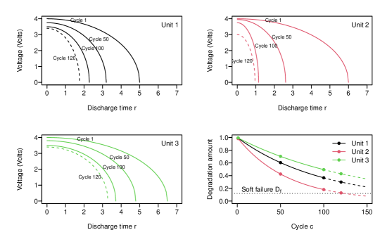
Figure 4: Degradation analysis diagram for multiple batteries. Panel 1 (top left), Panel 2 (top right), and Panel 3 (bottom left): Voltage discharge curves of each unit (battery). Solid curves are for modeling under procedure proposed in 3. Dashed curves are predictions based on final model. For each of these VDCs, degradation amount is measured according to equation (11). Panel 4 (bottom right): degradation paths for all units obtained from VDCs with observed (solid) and predicted (dashed) values overlayed with a soft failure threshold $D_{f}$.

4 Simulation Study

4.1 Existing degradation models

Current methods in degradation analysis of rechargeable batteries do not take into account the full functional form of VDCs. The observed VDCs are transformed into a scalar degradation measurement through equations (10) and (11). Then a general path model meeker2004degradation is constructed based on the observed degradation amount $d_{ic}$

$$d_{ic}=\mathcal{D}_{i}(c;{\boldsymbol{\beta}},\boldsymbol{\xi}_{i}|{\boldsymbol{z}}_{i})+\epsilon_{ic},$$ (12)

where ${\boldsymbol{z}}_{i}$ is the vector of covariates for battery $i$, $\mathcal{D}_{i}$ is a function of the cycle $c$ given ${\boldsymbol{z}}_{i}$ with parameters ${\boldsymbol{\beta}}$ and $\boldsymbol{\xi}$. In particular, ${\boldsymbol{\beta}}$ contains all the fixed parameters common across all batteries and $\mathbf{\xi}_{i}=(\xi_{1i},\dots,\xi_{i\ell})^{\top}$ collects $\ell$ random parameters representing battery-to-battery variations. In model (12), $\mathbf{\xi}_{i}$ is assumed to follow a multivariate normal distribution with mean $\mathbf{0}$ and covariance $\boldsymbol{\Sigma}$, and the random errors $\epsilon_{ic}$ are assumed to be independent and identically distributed, following a normal distribution with mean 0 and variance $\sigma^{2}_{\epsilon}$.

The first step in the degradation model (12) is specifying the functional form of $\mathcal{D}_{i}(c)$ based on the shape of the degradation path formed by the degradation amounts $d_{ic}$ along the cycles. Based on Figure 2, we use a linear degradation path of the form

$$\mathcal{D}_{i}(c)=\beta_{0}+(\beta_{1}+\xi_{i1})c+{\boldsymbol{z}}_{i}^{\top}\mathbf{\beta}_{z}.$$ (13)

By setting $\exp(\zeta_{i1})=|1+\xi_{i1}/\beta_{1}|$, we can see that model (13) has an equivalent form

$$\mathcal{D}_{i}(c)=\beta_{0}+\beta_{1}\exp(\zeta_{i1})c+{\boldsymbol{z}}_{i}^{\top}\mathbf{\beta}_{z},$$ (14)

where $\beta_{1}$ may differ from $\beta_{1}$ in (13) by a sign and the random effect $\zeta_{i1}$ now assumes a lognormal probability distribution. The goal is now to estimate parameters $\boldsymbol{\theta}=\{\boldsymbol{\beta}$, $\sigma^{2}_{\epsilon}$, $\boldsymbol{\Sigma}\}$. Note that in general model (12) is a nonlinear mixed-effects model, which can be estimated through standard methods such as maximum likelihood (ML) or REML. In practice, we apply the nlme and lme functions from the R package nlme pinheiro2017package.

4.2 Simulation settings

We conduct a numerical simulation study to compare degradation analysis performance between our functional data approach and existing methods. In numerical studies, we simulate data from a hypothetical experiment with $n$ number of units. For each $i=1,\ldots,n$, unit $i$ is set to go through $n_{i}$ cycles of action that result in its degradation. Within each cycle, a curve observation is simulated. This curve is assembled from two components: a curve on the standard $[0,1]$ domain and a domain end point that scales the standard curve to an individualized domain. In particular, the domain end point $b_{ic}$ for curve $c$ of unit $i$ is simulated from the following model

$$b_{ic}=\alpha_{0}+w_{0i}+(\alpha_{1}+w_{1i})c+\alpha_{2}x_{i}+\alpha_{3}b_{i,c-1}+\alpha_{4}\exp\left\{\frac{-1}{\Delta_{ic}}\right\}+\epsilon_{ic},$$ (15)

where $w_{0i}\sim\mathcal{N}(0,\sigma^{2}_{0})$, $w_{1i}\sim\mathcal{N}(0,\sigma^{2}_{1})$, $\epsilon_{ic}\sim\mathcal{N}(0,\sigma^{2}_{\epsilon})$. The covariate $x_{i}$ represents a testing condition for unit $i$, which is generated from a uniform distribution on $[0,1]$. The time lag $\Delta_{ic}$ between cycles $c-1$ and $c$ is set up as follows. When $c$ is divisible by 20, we set $\Delta_{ic}=100+\ell$ where $\ell\sim\mathcal{N}(0,2^{2})$. Otherwise, $\Delta_{ic}=5+\ell$, where $\ell\sim\mathcal{N}(0,1^{2})$. In this manner, we assume the hypothetical system has a long break every 20 cycles. Once $b_{ic}$ is generated, the curve $y_{ic}(r)$ with $r\in[0,b_{ic}]$ is obtained through $y_{ic}(r)=\sum_{j}^{3}\gamma_{ic,j}\phi_{ijc}(r)$, where $\phi_{ijc}(r)$ are the first three basis functions in the cubic B-spline basis system with 5 equally spaced knots on the interval $[0,b_{ic}]$. Models for the coefficients $\gamma_{ic,j},j=1,2,3$, are

$$\gamma_{ic,j}=(u_{01}+v_{0ij})+(u_{11}+v_{1ij})c+u_{2}x_{i}+\delta_{ic,j},$$ (16)

where $v_{0ij},v_{1ij}\sim\mathcal{N}(0,\sigma^{2}_{v})$ and $\delta_{icj}\sim\mathcal{N}(0,\sigma^{2}_{\delta})$.

With the guidance of the application, we choose our parameter values as follows. The fixed-effects coefficients in (15) are $\alpha_{0}=2500$, $\alpha_{1}=-5$, $\alpha_{2}=50$, $\alpha_{3}=0.5$, and $\alpha_{4}=150$. The variance of random effects and noise are $\sigma^{2}_{w0}=200^{2}$, $\sigma^{2}_{w1}=2^{2}$ and $\sigma^{2}_{\epsilon}=10^{2}$. In (16), the fixed effects are set as $(u_{01},u_{02},u_{03})^{\top}=(10,6,5)^{\top}$, $(u_{11},u_{12},u_{13})^{\top}=(-0.03,-0.02,-0.01)^{\top}$, and $(u_{21},u_{22},u_{23})^{\top}=(5,4,3)^{\top}$. The variances of random effects and noise are respectively $\sigma^{2}_{v}=0.01$ and $\sigma^{2}_{\delta}=1^{2}$. Figure 5 displays the data for a unit generated in this manner.

Figure 5: Example of simulated discharge curves through 100 discharge cycles for one unit. Colors ranging from blue to purple indicate increase in discharge cycle number. Left panel displays the curves in their original domain. Right panel is the scaled curves.

To test the efficacy of the proposed method on the simulated data, we build predictive models from the first $tr\%$ of the number of cycles of each unit. $tr\%$ is the chosen training data ratio. Predictions are done on the remaining $1-tr\%$. We choose the degradation measure of interest to be the normalized difference between the $L^{1}$-norms, or areas under the curves, of the VDCs at cycle $c$ and the first cycle, namely, $d_{ic}=\frac{\parallel y_{i1}(r)\parallel_{1}-\parallel y_{ic}(r)\parallel_{1}}{\parallel y_{i1}(r)\parallel_{1}}$. The accuracy in prediction is evaluated by the root mean squared prediction error $\textrm{RMSPE}=\sqrt{\sum_{i=1}^{n}\sum_{c=\tilde{n}_{i}}^{n_{i}}(\hat{d}_{ic}-d_{ic})^{2}}$ where $\tilde{n}_{i}=n_{i}\cdot tr\%+1$. We also evaluate the goodness of fit in estimating degradation amount using root mean squared error $\textrm{RMSE}=\sqrt{\sum_{i=1}^{n}\sum_{c=1}^{\tilde{n}_{i}-1}(\hat{d}_{ic}-d_{ic})^{2}}$.

Our simulation settings comprise of all the possible combinations of $n=\{20,50,100\}$, $n_{i}=\{50,100,150\}$, and train ratio $tr\%=\{50\%,80\%\}$. Each simulation setting contains 500 data replications. Model for general path modeling is fitted with the lme routine from the R package nlme. For the simulation study, we apply the linear degradation path in equation (13). For the proposed functional model approach, we apply the functional principal component decomposition from fdapace R package fdapace, then the multivariate linear mixed-effects model for FPC scores are constructed using lme on the vectorized form as demonstrated above. Two models of estimating EOD time are considered. The first is the linear mixed-effects model similar to (15). The second is the FLMM where we fit (15) with the covariate term $\alpha_{2}x_{i}$ replaced with the functional covariate $\int_{0}^{1}{\left(\beta(t)+b_{i}(t)\right)x_{ic}(t)dt}$. We customized the code provided in liu2017estimating to obtain the estimated parameters in the functional linear mixed model in model (7).

4.3 Simulation results

Figure 6 shows the boxplots of RMSPEs of the three methods grouped by simulation settings. Here, GPM stands for the general path model using the linear degradation path. Models using functional data approach are pre-fixed with FDM followed by the method of modeling EOD. From Figure 6, when the training ratio is $tr\%=80\%$ and number of cycles per battery at 50 and 100, the two FDM models, FDM-LME and FDM-FLMM, produce almost identical results and both are much better than the GPM method.

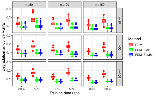
Figure 6: RMSPE over all simulation settings combinations from three degradation models.

We examine the goodness of fit for these models on the training data in Figure 7. It is not surprising that GPM has a better performance in fitting the training data compared to the two FDM models. The GPM directly models the degradation amounts. Although this yields better fit on training data, it also tends to overfit the data and thus leads to worse prediction performance as demonstrated above. On the other hand, the two FDM models deal with functional VDCs from two sources: the scaled VDCs and the EODs. Although the FDM approaches do not fit the training data as the direct GPM approach, they gain in the prediction performance which is more important in degradation analysis.

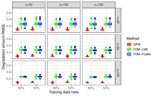
Figure 7: Boxplots of RMSE on observed data over all simulation settings combinations from three degradation models.

We examine the functional data models further by looking at the fit and prediction performance for scaled VDCs across different simulation settings in Figure 8. Using FPC scores to model scaled VDCs gives good fit based on pointwise MSE over all simulation settings. The discrepancy between fit and prediction MSE reduces as the number $n_{i}$ of cycles per battery increases. On the other hand, the increase in the number $n$ of batteries leads to smaller variances in prediction errors.

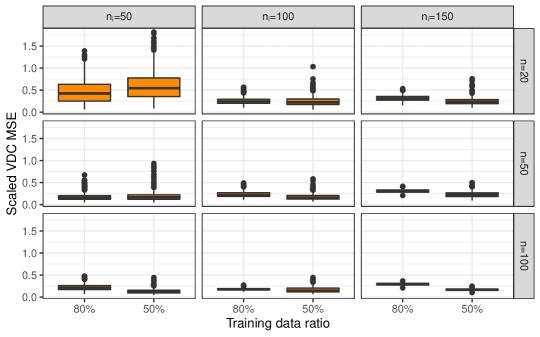
Figure 8: Boxplots of Point-wise MSE of scaled VDCs in training (Fit Type) and testing set (Pred. Type) over all simulation settings.

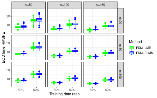
Figure 9: Boxplots of RMSPE of EOD time by FDM-LME and FDM-FLMM over all simulation settings.

Both FDM-LME and FDM-FLMM use the same method for modeling scaled VDCs through FPC scores. They differ in modeling the EOD time. Figure 9 displays boxplots of RMSPE for predicting EOD time by the two models. While the prediction performance of FDM-LME is slightly better for the case of small $n$ and $n_{i}$, the two methods produce almost identical results as the number of batteries and the number of cycles per battery increase. This explains the similarity in performance between the two models in Figure 6.

5 Data Analysis

5.1 Model construction

The dataset contains voltage discharge curves for $n=20$ batteries under various experimental conditions. The experimental conditions are respectively the testing temperature (temp) in Celsius degrees, discharge current (dc) in Amp, and the stopping voltage (sv) in volts. The number of cycles $n_{i}$ for a battery ranges from 60 to 200. For each discharge cycle, the end of discharge (EOD) $b_{ic}$ is defined to be the time elapsed from the beginning to the end of the cycle. To obtain the scaled curves $x_{ic}(t)$, we scale the timestamps on each voltage discharge curve (VDC) $y_{ic}(r)$ by the corresponding $b_{ic}$. Since the time grid for the scaled curve $x_{ic}(t)$ may differ between cycles and batteries, we interpolate each curve to obtain observations on a uniform grid. All the covariates are modeled as continuous variables. We apply the Arrhenius transformation for temperature using room temperature as the baseline level meeker2004degradation, that is

$$z_{1}=\frac{11604.52}{\text{\emph{temp}}^{\circ}\text{C}+273.15}-\frac{11604.52}{24^{\circ}\text{C}+273.15}.$$

For discharge current (dc) and stopping voltage sv, we use the following transformations,

$$z_{2}=\frac{\log(\text{\emph{dc}})}{2}\quad\mathrm{and}\quad z_{3}=\frac{\log(\emph{sv})}{2}.$$

This is called the power law transformation using 2 Amps as baseline level for discharge current and 2 Volts as baseline level for stopping voltage meeker2004degradation. These are standard transformations in battery studies and can enhance the numerical stability in model fitting. Furthermore, the baseline levels for the three experimental conditions have a covariate value of 0 under these transformations. This makes it easier to interpret the intercept of the model and compare the effects on the response between different levels of each covariate.

When performing the FPCA on the scaled VDCs, we find that the first three FPCs can already explain more than $99\%$ of the total variation in the curves. Therefore, we use $K=3$ here and represent each curve $x_{ic}(t)$ by the three corresponding FPC scores, $\gamma_{ic,j}$, $j=1,2,3$. We fit the multivariate linear mixed-effects model in (3) with ${\boldsymbol{z}}_{i}=(z_{1i},z_{2i},z_{3i})^{\top}$, using the procedure introduced in Section 3.

Once the model is fitted and the parameters are estimated, we apply

$$\hat{{\boldsymbol{\gamma}}}_{ic^{*}}=\hat{{\boldsymbol{v}}}_{0}+\hat{{\boldsymbol{u}}}_{0i}+(\hat{{\boldsymbol{v}}}_{1}+\hat{{\boldsymbol{u}}}_{1i})c^{*}+\hat{\mathbf{P}}{\boldsymbol{z}}_{i}$$ (17)

to obtain the predicted FPC scores of the scaled voltage discharge curves $x_{ic^{*}}(t)$ for a future cycle $c^{*}$. Combining these scores with the FPCs and the estimated mean discharge function $\hat{\mu}(t)$ yields the prediction of the scaled curve $x_{ic^{*}}(t)$ for cycle $c^{*}$.

The next step is to model the EOD time $b_{ic}$. Visual inspection in Figure 10 indicates that a linear trend in cycle number can capture well the trajectory of EOD time. To capture the variations between batteries, a reasonable model choice is the linear mixed-effects model with random terms for the intercept and slope for cycle number grouped by battery. Two additional covariates are introduced following the suggestion in saha2009pf. One is the EOD $b_{i,c-1}$ of the previous cycle, to capture the autoregressive nature of EODs found in their analysis. The other is a transformation of the waiting time $\Delta_{ic}$ between two cycles, namely, $\exp(-1/\Delta_{ic})$. Hence the first option to model $b_{ic}$ is the form of model (6) with ${\boldsymbol{z}}_{i}=(b_{i,c-1},\exp(-1/\Delta_{ic}),z_{1i},z_{2i},z_{3i})^{\top}$.

A second option is to take advantage of the information from scaled voltage discharge curve by fitting the functional linear mixed-effects model (7). Since the experimental conditions have already been incorporated into the model for $x_{ic}(t)$, we choose not to include them again in the models for the EOD time, and thus ${\boldsymbol{z}}_{i}$ in (7) becomes ${\boldsymbol{z}}_{i}=(b_{i,c-1},\exp(-1/\Delta_{ic}))^{\top}$. We first fit models (6) to (7) using the training data, that is, the first $tr\%$ of data for each battery. Based on the fitted models, we make predictions on the $1-tr\%$ held-out testing data.

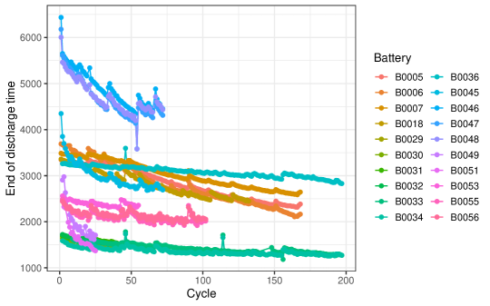
Figure 10: End of discharge (EOD) time per cycle by each battery.

After prediction of the scaled curve $x_{ic}(t)$ as well as domain end time $b_{ic}$, we reconstruct the curve on its natural domain $y_{ic}(s)$ and compute the degradation amount (11) using the $L^{p}$ norm with $p=1$. As done in simulations, we compare our degradation predictions to those from the general path model which is based only on the degradation amounts at the training cycles.

5.2 Model evaluation

We consider three levels for the train ratio, $tr\%\in\{50\%,75\%,90\%\}$. For illustrating purpose, we present the fitted and predicted degradation paths for the $75\%$ train ratio setting. Figure 11 displays the predicted degradation paths for 4 presenting batteries when $75\%$ of available data for each battery are used in modeling. Predictions from FDM-LME and FDM-FLMM are able to capture well the testing part trajectories of the degradation paths for most batteries while GPM tends to overestimate degradation amounts. Prediction for battery B0053 is an exception with all models perform badly. This is because of the big dip in the degradation path corresponding to a longer than normal resting period $\Delta_{ic}$. While all three models have built-in mechanism to capture this resting period, its effect is much more profound then the prediction from any model.

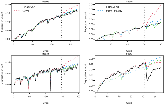
Figure 11: Degradation paths for 4 representing batteries (gray) overlayed with fitted and predicted paths by GPM (red), FDM-LME (green), and FDM-FLMM (blue). Dotted vertical line indicate the separation between train (first $75\%$ of discharge cycles from each battery) and test set (last $25\%$ of discharge cycles from each battery).

Figure 12 shows boxplots of absolute errors of the three methods when fitting and predicting degradation amount under the three train/test ratios. In contrast to the under-performance in fitting of the two FDM models versus the GPM in the simulation study, the fits on the training data from all three methods are quite consistent with one another. In prediction, both FDM models give better and more consistent performance than the GPM.

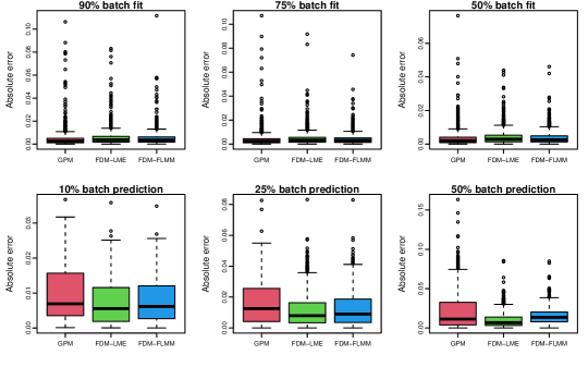
Figure 12: Boxplots of absolute error in degradation amount fit and prediction among three considered methods across three train/test split ratios.

5.3 Degradation prediction

Lastly, we perform functional degradation analysis using all the available data on the batteries, that is, we make prediction about the battery degradation beyond the discharge cycles available in the data. We use the results from the FDM-FLMM model as an example and predict the VDCs and degradation paths for the next 20 cycles of each battery assuming a 5-hour lag between cycles. Figure 13 visualizes the results for two batteries. This result illustrates the benefits of functional degradation model in producing both the predictions for VDCs and the degradation amount of interest.

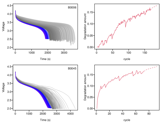
Figure 13: Predicted voltage discharge curves and degradation paths for two batteries in the next 20 discharge cycles based on FDM-FLMM model built on entire battery dataset.

6 Conclusion and Future Work

In this work, we propose a functional degradation model to analyze a battery life testing study, where voltage discharge curves form a longitudinal set of functional data observations showing a pattern of degradation. Instead of applying standard degradation models directly to degradation measures summarizing functional observations, our functional data approach take full advantage of the whole VDCs. Considering the heterogeneity in the supporting domains of the VDCs, we first re-scale each VDC to reside on the common domain $[0,1]$ and then simultaneously model the scaled curves and the EOD times through mixed-effects models. Simulations show that our functional degradation model can indeed yield better predictions than the standard general path model. Our detailed analysis of the battery life testing data further reveal the great potential of the functional degradation model for more accurate and more stable degradation prediction for Lithium-ion batteries. Another advantage of the functional approach is that its prediction is not only just a predicted value for the degradation amount but also a complete VDC. The availability of complete VDC predictions would allow the practitioners the flexibility of defining their own degradation measures based on the curves.

There are, however, potential assumptions in our models that may not be realistic and should be studied in a future work. First, we assume a linear effect from the experimental conditions. This might not be true from physical sciences especially with factors like temperature. Other aspects of variable selection should be an interesting topic to explore. The FLMM models also assume EOD time follows a normal distribution. While most EOD time is sufficiently far away from zero to safely be considered normal, it is still an assumption that needs to be examined in the future.

The degradation paths show interesting impact from resting period and accounting for the resting time helps improve local and overall prediction accuracy. Currently, in order to predict degradation in the future, resting time needs to be preset. This is not realistic. A better approach would be to account for randomness in resting amount. As seen in Figure 11, a long resting period in battery B0053 completely drive the data away from all models’ prediction. It would be beneficial to develop a guide on when to reset model training based on length of resting period. In addition, it will be interesting to consider time-varying covariates such as varying temperature, multiple current loading values, and stopping voltage levels that interchange across discharge cycles. The latter would be for a more realistic situation where batteries are discharge to half or a quarter of its voltage capacity instead of a full discharge like our current application.

Appendices

A.1 Interpretation of functional principal components for scaled discharge voltage curves

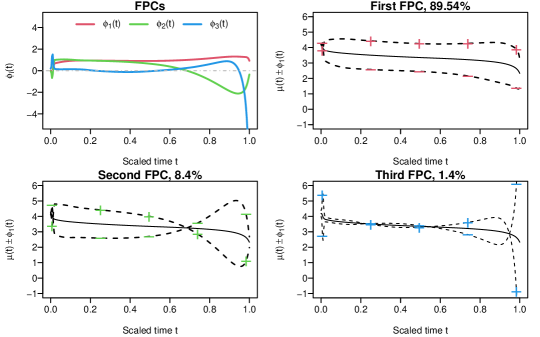
Figure 14: First three principal component functions with their proportion of total variation explained from FPC decomposition of scaled VDCs for available data from 20 batteries. Top left show the plots of the three principal components. Top right and the bottom two plots show the effect on the mean function (solid black) after adding and subtracting the FPCs.

Figure 14 visualizes the first three estimated functional principal components obtained from FPC decomposition of the scaled VDCs from all available discharge data. This decomposition result is used in Section 5.3. Visualizing the FPCs by adding and subtracting them from the mean curves helps illustrate their interpretation. The first FPC, accounting for $89.54\%$ of total variation in the data, is a positive function across the domain. Besides having values tapering toward 0 at the two ends, the first FPC is quite flat and its values consistent throughout the domain. The top right plot in Figure 14 suggests that scaled VDC with positive score for the first FPC have higher voltage than the average scaled VDC almost entirely throughout the domain or discharge cycle. On the other hand, scaled VDC with negative score has lower voltage level than the average scaled VDC on the entire domain. Hence, first FPC indicates the deviation from the mean scaled VDC. The sign and magnitude of the first FPC score quantify the direction and strength of this deviation.

The second FPC explains $8.4\%$ of total variation of the data. It has positive values approximately before $0.7$ mark and negative after that. It represents the difference in discharge voltage in the first $70\%$ of the cycle. This second FPC represents the contrast between voltage level in the first $70\%$ of the discharge cycle and the latter $30\%$. Scaled VDCs with high second FPC scores are those with higher than average voltage in the first $70\%$ of the discharge cycle but the voltage levels drop more significantly than the average in the remaining time of the cycle. Cycles with negative scores are those with lower voltage at the beginning of the cycle but the drop in later into the cycle is not as dramatic compared to the mean curve.

The third FPC shows close to 0 values for the majority of the cycle except for the beginning and end of the cycle. This represents the variation in the scaled VDCs in terms of the beginning voltage level and how voltage drop at the end of the discharge cycles.

A.2 Interpretation of estimates from functional linear mixed-effects model for EOD time

The model for end of discharge time $b_{ic}$ applied in Section 5.3 is

$$b_{ic}=\alpha_{0}+w_{0i}+(\alpha_{1}+w_{1i})c+\int_{0}^{1}\left(\beta(t)+b_{i}(t)\right)x_{ic}(t)dt+\alpha_{2}b_{i,c-1}+\alpha_{3}\exp(-1/\Delta_{ic})+\epsilon_{ic},$$ (18)

The estimations for fixed coefficients and their standard errors (se) are $\hat{\alpha}_{0}=-3845.733$ with se 931.087, $\hat{\alpha}_{1}=-1.687$ with se 0.38, $\hat{\alpha}_{2}=546.7246$ with se 25.2, and $\hat{\alpha}_{3}=0.59$ with se 0.014. Figure 15 illustrates the estimated coefficient function $\beta(t)$ of the effect of scaled VDCs on EOD plotted point-wise and Figure 16 shows the 20 battery-specific effect from scaled VDCs on EOD, $\beta(t)+b_{i}(t)$.

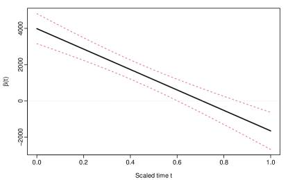
Figure 15: Point-wise estimated coefficient function of the effect from scaled VDC on EOD time, $\beta(t)$. Mean estimate is in the solid black curve and red dashed curves indicated the approximated $95\%$ confidence band.

Figure 16: Estimated functional coefficients of scaled VDC by battery from FLMM model predicting EOD time. Dashed curve represents overall coefficient function $\hat{\beta}(t)$. Battery-specific coefficient functions, $\hat{\beta}(t)+\hat{b}_{i}(t)$, are depicted by solid red curves

From the form of (18), the effect from the scaled VDCs is a weighted average of the scaled VDC with the weight set by the coefficient function $\beta(t)$ adjusted with $b_{i}(t)$ for each batter. The estimated $\beta(t)$ has the shape close to a straight line with negative slope and sign of values switch at around $0.7$. Recall the shape of a typical scaled VDCs (Figure 14), we can see that this term $\int_{0}^{1}\left(\beta(t)+b_{i}(t)\right)x_{ic}(t)dt$ acts as an adjustment to EOD based on a weighted average of scaled VDCs. Without battery specific effect $b_{i}(t)$, this adjustment is similar to an area under the curve. Depending on the battery, the variations in the shapes of scaled VDCs help set the weight to be $\beta(t)+b_{i}(t)$.

References

- [\citeauthoryearAneiros, Cao, Fraiman, Genest, and VieuAneiros et al.2019] Aneiros, G., R. Cao, R. Fraiman, C. Genest, and P. Vieu (2019). Recent advances in functional data analysis and high-dimensional statistics. Journal of Multivariate Analysis 170, 3–9.
- [\citeauthoryearBullBull2001] Bull, S. R. (2001). Renewable energy today and tomorrow. Proceedings of the IEEE 89(8), 1216–1226.
- [\citeauthoryearCarroll, Gajardo, Chen, Dai, Fan, Hadjipantelis, Han, Ji, Mueller, and WangCarroll et al.2021] Carroll, C., A. Gajardo, Y. Chen, X. Dai, J. Fan, P. Z. Hadjipantelis, K. Han, H. Ji, H.-G. Mueller, and J.-L. Wang (2021). fdapace: Functional Data Analysis and Empirical Dynamics. R package version 0.5.6.
- [\citeauthoryearCastelvecchi et al.Castelvecchi et al.2021] Castelvecchi, D. et al. (2021). Electric cars and batteries: how will the world produce enough? Nature 596(7872), 336–339.
- [\citeauthoryearDiouf and PodeDiouf and Pode2015] Diouf, B. and R. Pode (2015). Potential of lithium-ion batteries in renewable energy. Renewable Energy 76, 375–380.
- [\citeauthoryearHe, Shen, Shen, and MaHe et al.2015] He, Y.-J., J.-N. Shen, J.-F. Shen, and Z.-F. Ma (2015). State of health estimation of lithium-ion batteries: A multiscale gaussian process regression modeling approach. AIChE Journal 61(5), 1589–1600.
- [\citeauthoryearLi, Qiu, and XuLi et al.2022] Li, Y., Y. Qiu, and Y. Xu (2022). From multivariate to functional data analysis: Fundamentals, recent developments, and emerging areas. Journal of Multivariate Analysis 188, 104806. 50th Anniversary Jubilee Edition.
- [\citeauthoryearLiu, Wang, and CaoLiu et al.2017] Liu, B., L. Wang, and J. Cao (2017). Estimating functional linear mixed-effects regression models. Computational Statistics & Data Analysis 106, 153–164.
- [\citeauthoryearLiu, Luo, Liu, Peng, Guo, and PechtLiu et al.2014] Liu, D., Y. Luo, J. Liu, Y. Peng, L. Guo, and M. Pecht (2014). Lithium-ion battery remaining useful life estimation based on fusion nonlinear degradation ar model and rpf algorithm. Neural Computing and Applications 25(3), 557–572.
- [\citeauthoryearLiu, Luo, Peng, Peng, and PechtLiu et al.2012] Liu, D., Y. Luo, Y. Peng, X. Peng, and M. Pecht (2012). Lithium-ion battery remaining useful life estimation based on nonlinear ar model combined with degradation feature. In Annual Conference of the PHM Society, Volume 4.
- [\citeauthoryearLiu, Pang, Zhou, and PengLiu et al.2012] Liu, D., J. Pang, J. Zhou, and Y. Peng (2012). Data-driven prognostics for lithium-ion battery based on gaussian process regression. In Proceedings of the IEEE 2012 prognostics and system health management conference (PHM-2012 Beijing), pp. 1–5. IEEE.
- [\citeauthoryearLiu, Pang, Zhou, Peng, and PechtLiu et al.2013] Liu, D., J. Pang, J. Zhou, Y. Peng, and M. Pecht (2013). Prognostics for state of health estimation of lithium-ion batteries based on combination gaussian process functional regression. Microelectronics Reliability 53(6), 832–839.
- [\citeauthoryearLiu, Zhou, Pan, Peng, and PengLiu et al.2015] Liu, D., J. Zhou, D. Pan, Y. Peng, and X. Peng (2015). Lithium-ion battery remaining useful life estimation with an optimized relevance vector machine algorithm with incremental learning. Measurement 63, 143–151.
- [\citeauthoryearLuo, Lv, Wang, and LiuLuo et al.2011] Luo, W., C. Lv, L. Wang, and C. Liu (2011). Study on impedance model of li-ion battery. In 2011 6th IEEE Conference on Industrial Electronics and Applications, pp. 1943–1947. IEEE.
- [\citeauthoryearMartin, Ouwerkerk, Lamping, and CohenMartin et al.2022] Martin, J. A., J. N. Ouwerkerk, A. P. Lamping, and K. Cohen (2022). Comparison of battery modeling regression methods for application to unmanned aerial vehicles. Complex Engineering Systems.
- [\citeauthoryearMeeker, Hong, and EscobarMeeker et al.2004] Meeker, W., Y. Hong, and L. Escobar (2004). Degradation models and analyses. Encyclopedia of Statistical Sciences, 1–23.
- [\citeauthoryearNascimento, Corbetta, Kulkarni, and VianaNascimento et al.2021] Nascimento, R. G., M. Corbetta, C. S. Kulkarni, and F. A. Viana (2021). Hybrid physics-informed neural networks for lithium-ion battery modeling and prognosis. Journal of Power Sources 513, 230526.
- [\citeauthoryearNg, Xing, and TsuiNg et al.2014] Ng, S. S., Y. Xing, and K. L. Tsui (2014). A naive bayes model for robust remaining useful life prediction of lithium-ion battery. Applied Energy 118, 114–123.
- [\citeauthoryearOlabi and AbdelkareemOlabi and Abdelkareem2022] Olabi, A. and M. A. Abdelkareem (2022). Renewable energy and climate change. Renewable and Sustainable Energy Reviews 158, 112111.
- [\citeauthoryearPanwar, Kaushik, and KothariPanwar et al.2011] Panwar, N., S. Kaushik, and S. Kothari (2011). Role of renewable energy sources in environmental protection: A review. Renewable and sustainable energy reviews 15(3), 1513–1524.
- [\citeauthoryearPatil, Tagade, Hariharan, Kolake, Song, Yeo, and DooPatil et al.2015] Patil, M. A., P. Tagade, K. S. Hariharan, S. M. Kolake, T. Song, T. Yeo, and S. Doo (2015). A novel multistage support vector machine based approach for li ion battery remaining useful life estimation. Applied energy 159, 285–297.
- [\citeauthoryearPinheiro, Bates, DebRoy, Sarkar, Heisterkamp, Van Willigen, and MaintainerPinheiro et al.2017] Pinheiro, J., D. Bates, S. DebRoy, D. Sarkar, S. Heisterkamp, B. Van Willigen, and R. Maintainer (2017). Package ‘nlme’. Linear and nonlinear mixed effects models, version 3(1).
- [\citeauthoryearRamsay and SilvermanRamsay and Silverman1997] Ramsay, J. O. and B. W. Silverman (1997). Functional data analysis (1st Ed.). Springer Science Business Media.
- [\citeauthoryearRichardson, Osborne, and HoweyRichardson et al.2017] Richardson, R. R., M. A. Osborne, and D. A. Howey (2017). Gaussian process regression for forecasting battery state of health. Journal of Power Sources 357, 209–219.
- [\citeauthoryearSaha and GoebelSaha and Goebel2007] Saha, B. and K. Goebel (2007). Battery data set, nasa ames prognostics data repository (http://ti. arc. nasa. gov/project/prognostic-data-repository). NASA Ames Research Center, Moffett Field, CA. NASA AMES Prognostics Data Repository.
- [\citeauthoryearSaha and GoebelSaha and Goebel2009] Saha, B. and K. Goebel (2009). Modeling li-ion battery capacity depletion in a particle filtering framework. In Annual Conference of the PHM Society, Volume 1.
- [\citeauthoryearSaha, Goebel, and ChristophersenSaha et al.2009] Saha, B., K. Goebel, and J. Christophersen (2009). Comparison of prognostic algorithms for estimating remaining useful life of batteries. Transactions of the Institute of Measurement and Control 31(3-4), 293–308.
- [\citeauthoryearSaha, Goebel, Poll, and ChristophersenSaha et al.2008] Saha, B., K. Goebel, S. Poll, and J. Christophersen (2008). Prognostics methods for battery health monitoring using a bayesian framework. IEEE Transactions on instrumentation and measurement 58(2), 291–296.
- [\citeauthoryearSbarufatti, Corbetta, Giglio, and CadiniSbarufatti et al.2017] Sbarufatti, C., M. Corbetta, M. Giglio, and F. Cadini (2017). Adaptive prognosis of lithium-ion batteries based on the combination of particle filters and radial basis function neural networks. Journal of Power Sources 344, 128–140.
- [\citeauthoryearShah, Laird, and SchoenfeldShah et al.1997] Shah, A., N. Laird, and D. Schoenfeld (1997). A random-effects model for multiple characteristics with possibly missing data. Journal of the American Statistical Association 92(438), 775–779.
- [\citeauthoryearShen, Shen, and XuShen et al.2018] Shen, Y., L. Shen, and W. Xu (2018). A wiener-based degradation model with logistic distributed measurement errors and remaining useful life estimation. Quality and Reliability Engineering International 34(6), 1289–1303.
- [\citeauthoryearTagade, Hariharan, Ramachandran, Khandelwal, Naha, Kolake, and HanTagade et al.2020] Tagade, P., K. S. Hariharan, S. Ramachandran, A. Khandelwal, A. Naha, S. M. Kolake, and S. H. Han (2020). Deep gaussian process regression for lithium-ion battery health prognosis and degradation mode diagnosis. Journal of Power Sources 445, 227281.
- [\citeauthoryearTang, Yu, Wang, Guo, and SiTang et al.2014] Tang, S., C. Yu, X. Wang, X. Guo, and X. Si (2014). Remaining useful life prediction of lithium-ion batteries based on the wiener process with measurement error. energies 7(2), 520–547.
- [\citeauthoryearThiébaut, Jacqmin-Gadda, Chêne, Leport, and CommengesThiébaut et al.2002] Thiébaut, R., H. Jacqmin-Gadda, G. Chêne, C. Leport, and D. Commenges (2002). Bivariate linear mixed models using sas proc mixed. Computer methods and programs in biomedicine 69(3), 249–256.
- [\citeauthoryearWang, Chiou, and MüllerWang et al.2016] Wang, J.-L., J.-M. Chiou, and H.-G. Müller (2016). Functional Data Analysis. Annual Review of Statistics and Its Application 3(1), 257–295.
- [\citeauthoryearYu, Zhang, Qi, and LiYu et al.2022] Yu, Z., Y. Zhang, L. Qi, and R. Li (2022). Soh estimation method for lithium-ion battery based on discharge characteristics. International Journal of Electrochemical Science 17(220725), 2.