Correlation matrix of equi-correlated normal population: fluctuation of the largest eigenvalue, scaling of the bulk eigenvalues, and stock market

Abstract

Given an $N$-dimensional sample of size $T$ and form a sample correlation matrix $\mathbf{C}$. Suppose that $N$ and $T$ tend to infinity with $T/N$ converging to a fixed finite constant $Q>0$. If the population is a factor model, then the eigenvalue distribution of $\mathbf{C}$ almost surely converges weakly to Marčenko-Pastur distribution such that the index is $Q$ and the scale parameter is the limiting ratio of the specific variance to the $i$-th variable $(i\to\infty)$. For an $N$-dimensional normal population with equi-correlation coefficient $\rho$, which is a one-factor model, for the largest eigenvalue $\lambda$ of $\mathbf{C}$, we prove that $\lambda/N$ converges to the equi-correlation coefficient $\rho$ almost surely. These results suggest an important role of an equi-correlated normal population and a factor model in (Laloux et al. Random matrix theory and financial correlations, Int. J. Theor. Appl. Finance, 2000): the histogram of the eigenvalue of sample correlation matrix of the returns of stock prices fits the density of Marčenko-Pastur distribution of index $T/N$ and scale parameter $1-\lambda/N$. Moreover, we provide the limiting distribution of the largest eigenvalue of a sample covariance matrix of an equi-correlated normal population. We discuss the phase transition as to the decay rate of the equi-correlation coefficient in $N$.

1 Introduction

For risk management and asset allocation, a sample correlation matrix is essential. One of the pillars of Markowitz portfolio theory (Markowitz, 1959; Elton et al., 2014) is the study of correlation (or covariance) matrices, e.g., the optimal weight of each financial asset, given a set of assets with average returns and risks, so that the overall portfolio offers the best return for a fixed level of risk or, alternatively, the smallest risk for a given overall return. For these optimizations, the eigenvalues of covariance/correlating matrices are important. However, the eigenvalues of a sample covariance matrix/correlation matrix in finance are dispersed with noise, so various ways to eliminate noisy eigenvalues from them are studied by Laloux et al. (2000), El Karoui (2008), Ledoit & Wolf (2004, 2012), Ledoit & Péché (2011), Donoho et al. (2018), to cite a few. For this purpose, Laloux et al. (2000) proposed to approximate heuristically the distribution of noisy eigenvalues of a sample covariance/correlation matrix, with Marčenko-Pastur distribution (Marčenko & Pastur, 1967) of random matrix theory. Their idea influenced on the statistical methods on vaccine design (Quadeer et al., 2018). We will discuss the heuristic of Laloux et al. (2000) mathematically, with an equi-correlated normal population, which plays an important role in various risk models such as dynamic equicorrelation (Engle & Kelly, 2012) and constant correlation model (Elton et al., 2014).

First of all, we fix the notation. Let $\bm{X}_{1},\ldots,\bm{X}_{T}\in{{\mathbb{R}}}^{N}$ be a random sample. By the data matrix, we mean ${\mathbf{X}}=[\bm{X}_{1},\ldots,\bm{X}_{T}]\in{{\mathbb{R}}}^{N\times T}$. Let ${{1\leq i\leq N}}$ and ${{1\leq t\leq T}}$. The $it$-entry of ${\mathbf{X}}$ is denoted by $x_{it}$, and the $i$-th row by $\bm{x}_{i}\in{{\mathbb{R}}}^{1\times T}$. For the sample average of $\bm{x}_{i}$, write $\overline{x}_{i}=T^{-1}{\sum_{t=1}^{T}}x_{it}$. Let ${\overline{\bm{x}}}_{i}:=[\overline{x}_{i},\ldots,\overline{x}_{i}]\in{{\mathbb{R}}}^{1\times T}$ and $\overline{\mathbf{X}}:=[\overline{x}_{1},\ldots,\overline{x}_{N}]^{\top}[1,\ldots,1]\in{{\mathbb{R}}}^{N\times T}$. The sample correlation matrix is, by definition,

$$\mathbf{C} ={\mathbf{Y}}{\mathbf{Y}}^{\top}\in{{\mathbb{R}}}^{N\times N}\ \text{where}\ {\mathbf{Y}}^{\top}=\left[\frac{(\bm{x}_{1}-{\overline{\bm{x}}}_{1})^{\top}}{\lVert\bm{x}_{1}-{\overline{\bm{x}}}_{1}\rVert},\ldots,\frac{(\bm{x}_{N}-{\overline{\bm{x}}}_{N})^{\top}}{\lVert\bm{x}_{N}-{\overline{\bm{x}}}_{N}\rVert}\right].$$

Here, the notation $\lVert.\rVert$ is the Euclidean norm. The sample covariance matrix is denoted by $\mathbf{S}=T^{-1}{\mathbf{X}}{\mathbf{X}}^{\top}\in{{\mathbb{R}}}^{N\times N}$. By a distribution function, we mean a nondecreasing, right-continuous function $F:{{\mathbb{R}}}\to[0,1]$ such that $\lim_{x\to-\infty}F(x)=0$ and $\lim_{x\to+\infty}F(x)=1$.

We review the results on eigenvalue distributions from random matrix theory. The empirical spectral distribution of a symmetric matrix ${\mathbf{P}}\in{{\mathbb{R}}}^{N\times N}$ is, by definition,

$$F^{{\mathbf{P}}}(x)=\dfrac{1}{N}\#\Set{i\,\colon\,{{1\leq i\leq N}},\ \lambda_{i}({\mathbf{P}})\leq x}\quad(x\in{{\mathbb{R}}})$$

where $\lambda_{1}({\mathbf{P}}),\ldots,\lambda_{N}({\mathbf{P}})$ are the eigenvalues of ${\mathbf{P}}$, indexed in nonincreasing order. According to (Yao et al., 2015; Bai & Silverstein, 2010, p. 10), Marčenko-Pastur distribution with the sample size to dimension ratio index $Q>0$ and scale parameter $\sigma^{2}\in(0,\,\infty)$ has a density

$$\frac{Q}{2\pi\sigma^{2}x}\sqrt{(\sigma^{2}b_{Q}-x)(x-\sigma^{2}a_{Q})}1_{x\in[\sigma^{2}a_{Q},\,\sigma^{2}b_{Q}]}$$ (1)

and has a point mass of value $1-Q$ at the origin if $Q<1$. Here, $a_{Q}={(1-\sqrt{1/Q})^{2}}$,

$$b_{Q}={(1+\sqrt{1/Q})^{2}},$$

and $1_{\cdots}$ denotes the indicator function. Marčenko-Pastur distribution has expectation $\sigma^{2}$. The distribution function of Marčenko-Pastur distribution of the sample to dimension ratio index $Q$ and scale parameter $\sigma^{2}$ is denoted by $\mathrm{MP}_{Q,\sigma^{2}}$. We write $\mathrm{MP}_{Q}$ for $\mathrm{MP}_{Q,1}$. Clearly, $\mathrm{MP}_{Q,\sigma^{2}}(x)=\mathrm{MP}_{Q}(x/\sigma^{2})$ for all $x\in{{\mathbb{R}}}$. We say a sequence $(F_{i})_{i}$ of distribution functions converges weakly to a function $F$, if $F_{i}(x)\to F(x)$ for every $x\in{{\mathbb{R}}}$ where $F$ is continuous.

Proposition 1.1.

Let $\set{x_{it}\colon\,i,t\geq 1}$ be a double array of i.i.d. random variables with $\operatorname{E}|x_{11}|^{2}=\sigma^{2}\in(0,\,\infty)$. Suppose ${{N,T\to\infty,\ {T/N\to Q}}}\in(0,\,\infty)$. Then, almost surely,

1. $F^{\mathbf{S}}$ converges weakly to $\mathrm{MP}_{Q,\sigma^{2}}$. (Yao et al., 2015, p. 12)

2. $F^{\mathbf{C}}$ converges weakly to $\mathrm{MP}_{Q}$. (Jiang, 2004, Theorem 1.2)

However, the eigenvalues of financial correlation matrices distribute similarly as the random matrix theory suggests, but somehow differently. Laloux et al. (2000) considered a sample correlation matrix $\mathbf{C}$ “associated to the time series of the different stocks of the S&P500 (or other major markets)” where $N$ is the number of assets and $T$ is the number of observations. Laloux et al. (2000) found that the histogram of the eigenvalues of the financial, sample correlation matrix $\mathbf{C}$ fits not the density of $\mathrm{MP}_{T/N}$, but a scaled density, specifically, the density of

$$\mathrm{MP}_{\frac{T}{N},\,1-\frac{\lambda_{1}(\mathbf{C})}{N}}.$$ (2)

In addition to the fitting result, for the first eigenvalue $\lambda_{1}(\mathbf{C})$ of $\mathbf{C}$, Laloux et al. remarked the following:

The corresponding eigenvector is, as expected, the “market” itself, i.e., it has roughly equal components on all the $N$ stocks.

Laloux et al. (2000) interpreted the support of the density function of the fitting Marčenko-Pastur distribution, as the interval of noisy eigenvalues of the sample correlation matrix $\mathbf{C}$. Based on the findings of Laloux et al. (2000), in order to improve risk management, Bun et al. (2017) proposed “eigenvalue clipping: all eigenvalues in bulk of the fitting Marčenko-Pastur spectrum are deemed as noise and thus replaced by a constant value whereas the principal components outside of the bulk (the spikes) are left unaltered.” As portfolios of hundreds or thousands of assets becomes the target of research, many approaches have been proposed to deal with the problem of dimensionality. By the limiting regime ${{N,T\to\infty,\ {T/N\to Q}}}\in(0,\infty)$ of Proposition 1.1, we would like to understand mathematically why the heuristic of Laloux et al. (2000) is meaningful.

Let us hypothesize about the population of the stock prices Laloux et al. considered, from their remark on the eigenvector that “has roughly equal components on all the $N$ stocks.” It is comparable to an eigenvector $[1,\ldots,1]^{\top}$ corresponding to the largest eigenvalue $\lambda_{1}({\mathbf{\Sigma}}_{\rho})$ of an equi-correlation matrix

$${\mathbf{\Sigma}}_{\rho}=\begin{bmatrix}1&\rho&\cdots&\rho\\ \rho&1&\cdots&\rho\\ \vdots&\vdots&&\vdots\\ \rho&\rho&\cdots&1\end{bmatrix}\in{{\mathbb{R}}}^{N\times N}\qquad(0\leq\rho<1),$$

where

$$\lambda_{1}({\mathbf{\Sigma}}_{\rho})=(N-1)\rho+1\geq\lambda_{2}({\mathbf{\Sigma}}_{\rho})=\cdots=\lambda_{N}({\mathbf{\Sigma}}_{\rho})=1-\rho.$$ (3)

SenGupta (1988) studied hypothesis tests on $\rho=0$ vs. $\rho>0$. Ishii et al. (2021) developed nonparametric tests of the high-dimensional covariance structures such as a scaled identity matrix, a diagonal matrix and ${\mathbf{\Sigma}}_{\rho}$ for $N>T$ cases.

In particular, when $\rho>0$, $\lambda_{1}({\mathbf{\Sigma}}_{\rho})$ is unbounded with respect to $N$, and thus there is a ‘spectral gap’ between $\lambda_{1}({\mathbf{\Sigma}}_{\rho})=(N-1)\rho+1$ and $\lambda_{2}({\mathbf{\Sigma}}_{\rho})=1-\rho$. We presume that the population is a normal population with the population correlation matrix ${\mathbf{\Sigma}}_{\rho}$.

Then, for an equi-correlated normal population, we established the following scaling theorem for the limiting distribution of the bulk eigenvalues of the sample correlation matrix $\mathbf{C}$:

Proposition 1.2 (Akama & Husnaqilati (2022)).

Let $\mathbf{C}$ be a sample correlation matrix formed from an $N$-dimensional normal population such that the population correlation matrix is ${\mathbf{\Sigma}}_{\rho}$ with deterministic $\rho\in[0,\,1)$. Suppose ${{N,T\to\infty,\ {T/N\to Q}}}\in(0,\,\infty)$. Then, almost surely, the empirical spectral distribution $F^{\mathbf{C}}$ converges weakly to

$$\mathrm{MP}_{Q,\,1-\rho}.$$

It is worth noting that the limiting spectral distribution (LSD) $\mathrm{MP}_{Q,\,1-\rho}$ is similar to Marčenko-Pastur distribution (2) $\mathrm{MP}_{T/N,\,1-\lambda_{1}(\mathbf{C})/N}$ where the histogram of the eigenvalues of a financial correlation matrix fits to the density of (2). The index $Q$ and the scale parameter $1-\rho$ correspond to $T/N$ and $1-\lambda_{1}(\mathbf{C})/N$, respectively.

By comparing (2) to Proposition 1.2, we will show that the largest eigenvalue $\lambda_{1}(\mathbf{C})$ of the sample correlation matrix $\mathbf{C}$ divided by the order $N$ of $\mathbf{C}$ converges almost surely to the equi-correlation coefficient $\rho$, as follows. Hereafter, ${\stackrel{{\scriptstyle a.s.}}{{\to}}}$ and ${\stackrel{{\scriptstyle D}}{{\to}}}$ mean the almost sure convergence and the convergence in distribution respectively. Unless otherwise stated, the limiting regime is ${{N,T\to\infty,\ {T/N\to Q}}}\in(0,\,\infty)$.

Theorem 1.3.

Suppose the assumptions of Proposition 1.2. Then,

1. $\lambda_{1}(\mathbf{C})\big{/}{N}\mathrel{\stackrel{{\scriptstyle a.s.}}{{\to}}}\rho$.

2. If, moreover, the population is $\mathrm{N}_{N}(\bm{0},\ {\mathbf{\Sigma}}_{\rho})$ and $\rho>0$, then

   $$\frac{\lambda_{1}(\mathbf{S})-\tau}{\varsigma}\ {\stackrel{{\scriptstyle D}}{{\to}}}\ \mathrm{N}(0,1)$$

   where

   $$\tau=\frac{\left((N-1)\rho+1\right)\left(\left(1+(T-1)N\right)\rho+N-1\right)}{NT\rho},\quad\varsigma=\frac{(N-1)\rho+1}{\sqrt{2T}}.$$

From the first assertion, i.e., the consistency of $\lambda_{1}(\mathbf{C})/N$, of Theorem 1.3, Proposition 1.2 suggests that an equi-correlated normal population plays a role in Laloux et al.’s fitting result to the density of (2):

Corollary 1.4.

Assume the assumptions of Proposition 1.2. Then,

$$F^{\mathbf{C}}(x)-\mathrm{MP}_{\frac{T}{N},\,1-\frac{\lambda_{1}(\mathbf{C})}{N}}(x)\mathrel{\stackrel{{\scriptstyle a.s.}}{{\to}}}0\quad(x\neq 0).$$

Once the largest eigenvalue $\lambda_{1}(\mathbf{C})$ of $\mathbf{C}$ is found, Corollary 1.4 can suggest the support of the density of the fitting Marčenko-Pastur distribution to clean up (“eigenvalue clipping”), and then we can eliminate the eigenvalues in the support to let a small, but important eigenvalue (e.g., Markowitz solution) show up. Moreover, $\lambda_{1}(\mathbf{C})$ has been concerned by Friedman & Weisberg (1981).

The rest of the paper is organized as follows. In the next section, to generalize Proposition 1.2, we consider suitable factor models. Then, we establish the limiting spectral distribution of the sample correlation matrix $\mathbf{C}$ generated from such a factor model. In Section 3, for returns of S&P stock prices (2012-1-4/2021-12-31), we compute the largest eigenvalues of financial correlation matrices $\mathbf{C}$ divided by the order, and estimate the time average $\overline{\rho}$ of equi-correlation coefficient by GJR GARCH (Glosten et al., 1993) with the correlation structure being ‘equicorrelation’ (Engle & Kelly, 2012). We show that $\lambda_{1}(\mathbf{C})/N$ predicts very well $\overline{\rho}$. In Section 4, for a nonnormal population with equicorrelation coefficient $\rho=\rho_{N}$ decaying in $N$, we review the consistency and the asymptotic normality of $\lambda_{1}(\mathbf{S})$, by citing Yata & Aoshima (2009). Then, for the limiting distribution of an appropriate scaling of a translation of $\lambda_{1}(\mathbf{S})$ of equi-correlated normal population, we discuss the phase transition from the normal population to Tracy-Widom distribution (Baik et al., 2005), as to the decay rate of $\rho_{N}$. The proofs of Theorem 1.3, Corollary 1.4, and Theorem 2.3 are postponed in Section 5, Section 6, and Section 7, respectively, for the sake of the presentation.

2 From equi-correlated normal population to factor models in limit

Proposition 1.2 was proved by the following well-known fact (Fan & Jiang, 2019, (3.21)): Assume that $\bm{X}_{1},\ldots,\bm{X}_{T}\stackrel{{\scriptstyle\mbox{{i.\@i.\@d.\@}}}}{{\sim}}\mathrm{N}_{N}(\bm{0},\,{\mathbf{\Sigma}}_{\rho})$, $0\leq\rho<1$, and $[\bm{X}_{1},\ldots,\bm{X}_{T}]=[x_{it}]_{it}\in{{\mathbb{R}}}^{N\times T}$. Then, there are independent standard normal random variables ${{f}}_{t}$, $e_{it}$ $({{1\leq i\leq N}},\ {{1\leq t\leq T}})$ such that

$$x_{it}=\sqrt{\rho}{{f}}_{t}+\sqrt{1-\rho}e_{it}.$$ (4)

Actually, an equi-correlated normal population is a factor model (Bai, 2003; Mulaik, 2009) consisting of 1 factor. See Example 2.2. Beside this 1-factor model, a 3-factor model and a 5-factor model are employed by Fama & French (1993, 2015) to describe stock returns in asset pricing and portfolio management.

Bai (2003) studied an inferential theory for a general factor model of large dimensions to which classical factor analysis does not apply, by using limiting regime $N,T\to\infty,\sqrt{N}/T\to 0$. He derived the limiting distributions of the estimated factors and estimated factor loadings, the asymptotic normality of estimated common components, and their convergence rates. The convergence rate of the estimated factors and factor loadings can be faster than that of the estimated common components. These achievements are obtained under liberal conditions that allow for correlations and heteroskedasticities. Stronger results are obtained when the idiosyncratic errors are serially uncorrelated and homoskedastic. A necessary and sufficient condition for consistency of the estimated factors is derived for large $N$ but fixed $T$.

We will study a factor model in the limiting regime $N,T\to\infty,\ T/N\to Q$. First, we recall a factor model (Bai, 2003; Mulaik, 2009):

Definition 2.1.

For a nonnegative integer $K$, by a $K$-factor model, we mean a data matrix

$$\left[x_{it}\right]_{it}\in{{\mathbb{R}}}^{N\times T}$$

such that

$$x_{it}=\mu_{i}+\bm{\ell}_{i}{{\bm{f}}}_{t}+e_{it}\quad(1\leq i\leq N,\ 1\leq t\leq T),$$

$$\mbox{$\mu_{i}$ is a deterministic constant,}\qquad\qquad\qquad\qquad\qquad\ \qquad\qquad\qquad\qquad(\mbox{\emph{mean}})$$

$$\mbox{${\bm{\ell}}_{i}=[\ell_{i1},\ldots,\ell_{iK}]$ is a $K$-dimensional row vector,}\qquad\qquad\qquad(\mbox{\emph{factor loadings}})$$

$$\mbox{${{\bm{f}}}_{t}=[f_{t1},\ldots,f_{tk}]^{\top}$ is a $K$-dimensional column vector,}\qquad\quad(\mbox{\emph{common factors}})$$

$$\mbox{$f_{tk}$ $(1\leq t\leq T,\ 1\leq k\leq K)$ are centered, i.i.d. with $\operatorname{Var}f_{t1}=1$},$$

$$\mbox{$e_{it}$ $(1\leq t\leq T)$ are centered, i.i.d., for each $i$ $(1\leq i\leq N)$},$$

$$\mbox{$f_{tk}$ and $e_{it}$ $(1\leq i\leq p,\ 1\leq t\leq T,\ 1\leq k\leq K)$ are independent},\ \mbox{and}$$

$$\psi_{i}:=\operatorname{Var}e_{it}<\infty\quad\quad\quad\quad\quad\quad\quad\quad\quad\qquad\qquad\qquad\qquad\qquad(\mbox{\emph{specific variance}}).$$

$e_{it}$’s are called idiosyncratic components. $K$ is the number of factors.

Example 2.2.

The decomposition (4) is a factor model such that $K=1$, $\mu_{i}:=0$, $\ell_{i1}=\sqrt{\rho}$, $\psi_{i}:=1-\rho$, and both of $f_{t1}$ and $e_{it}$ are independent and normal.

$e_{it}$ $(i,t\geq 1)$ are i.i.d., and ${\bm{\ell}}_{i}\to\bm{\ell}$ for some $K$-dimensional row vector $\bm{\ell}$. In this case, define

$$\sigma_{\infty}^{2}:=\lim_{i\to\infty}\operatorname{Var}x_{it}=\lVert\bm{\ell}\rVert^{2}+\psi_{1}<\infty,\qquad\rho:=\frac{\lVert\bm{\ell}\rVert^{2}}{\lVert\bm{\ell}\rVert^{2}+\psi_{1}}.$$

Then, $1-\rho$ is the portion of the specific variance to the limiting total variance $\sigma_{\infty}^{2}$ of a variable $x_{it}$ $(i\to\infty)$.

The following generalizes Proposition 1.2. The LSD of a sample correlation matrix $\mathbf{C}$ generated from a factor model is as follows:

Theorem 2.3.

Given a factor model. Suppose ${{N,T\to\infty,\ {T/N\to Q}}}\in(0,\,\infty)$ and Assumption 2. Then, almost surely, $F^{\mathbf{C}}$ converges weakly to $\mathrm{MP}_{Q,\,1-\rho}$.

By Example 2.2, this generalizes Proposition 1.2. Theorem 2.3 is proved in Section 7.

3 The largest eigenvalue of financial correlation matrix

For a dataset of returns of $N$ S&P500 stocks (or other major markets) for $T$ trading days, Laloux et al. (2000) fitted the histogram of the eigenvalues of the correlation matrix $\mathbf{C}$, to the density function of a scaled Marčenko-Pastur distribution.

Naturally, the return of a stock is more correlated with the return of a stock of the same industry classification sector, than with the return of a stock of a different industry classification sector. We consider the 11 global industry classification standard (GICS) sectors of S&P500 stocks. For each GICS, for the dataset of the stock returns for the period 2012-01-04/2021-12-31, the time series of the equi-correlation coefficient is computed by GJR GARCH (Glosten et al., 1993) with the correlation structure being dynamic equicorrelation (Engle & Kelly, 2012) (We abbreviate this model to ‘GJR GARCH-DECO’). The program is due to Candila (2021).

However, the computation time of the time series of the equi-correlation coefficient by GJR GARCH-DECO is large, although we can quickly compute the estimator $\lambda_{1}(\mathbf{C})/N$ of the equi-correlation coefficient by a power method. For each dataset, we compare the time series to $\lambda_{1}(\mathbf{C})/N$ of the correlation matrix $\mathbf{C}$.

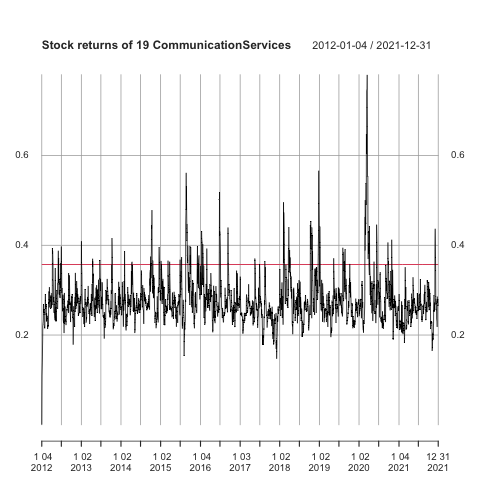
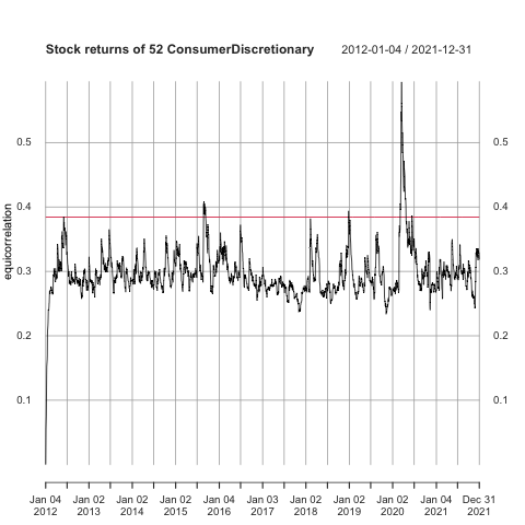
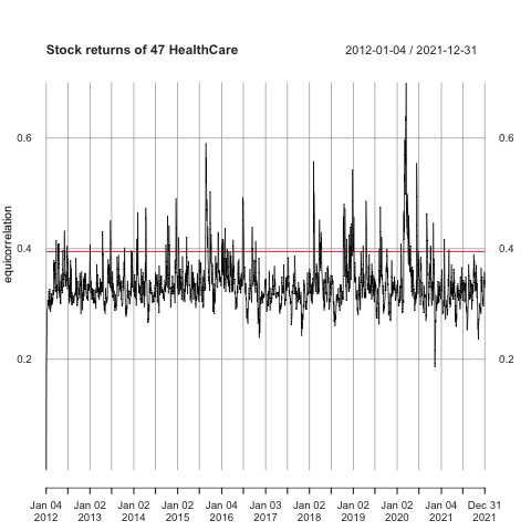
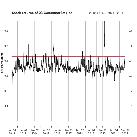
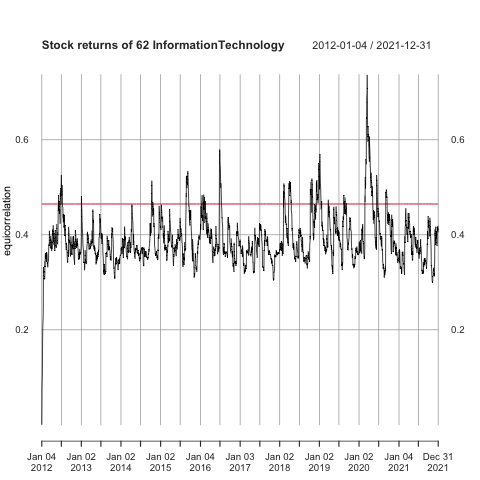
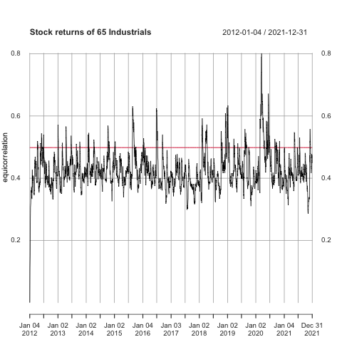
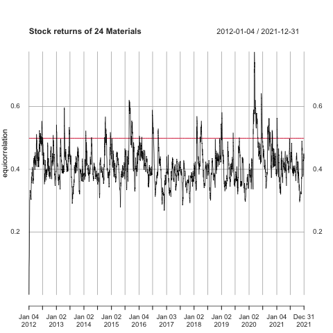
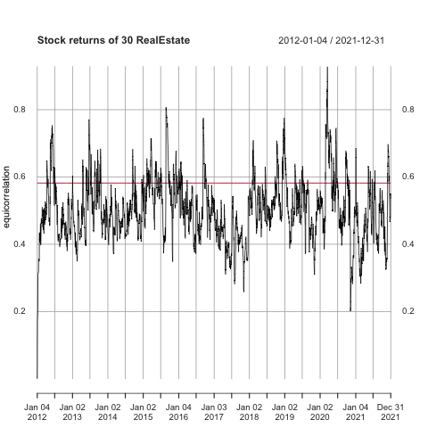
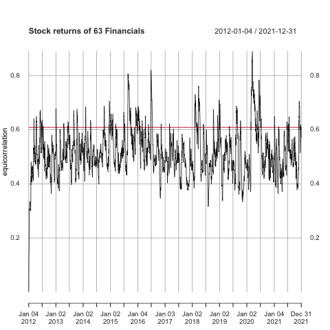
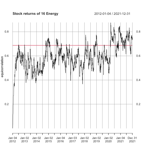
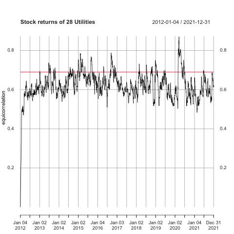
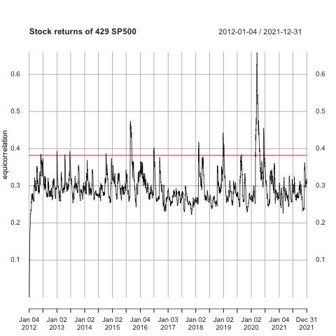
Figure 1: Time series of $\rho$ and $\lambda_{1}(\mathbf{C})/N$ (red line) of the stock returns of the 12 datasets of Table 1.

Figure 1 is the time series of equi-correlations for the 12 datasets. All the time series rise around March 2020, by the world-wide sudden crash after growing uncertainty due to the COVID-19 (Coronavirus disease 2019) pandemic. The time series of the equi-correlation coefficient of Energy sector kept high, even after the time series of the equi-correlation of the other 10 sectors of GICS as well as the total decrease. According to Figure 1, for each dataset, the time series is mostly smaller than $\lambda_{1}(\mathbf{C})/N$. Let us consider the time average $\overline{\rho}$ of equi-correlation coefficients estimated by GJR GARCH-DECO. Table 1 is the list of GICS, $N/T$, $\lambda_{1}(\mathbf{C})/N$, $N$, and $\overline{\rho}$, for the period 2012-01-04/2021-12-31 ($T=2516$=trading days $-1$). The rows of Table 1 are ordered in the increasing order of $\lambda_{1}(\mathbf{C})/N$.

No	GICS	$N/T$	$\lambda_{1}(\mathbf{C})/N$	$N$	$\overline{\rho}$
1	Communication Services	.0076	.3571	19	.2764
2	Consumer Discretionary	.0207	.3843	52	.2967
3	Health Care	.0187	.3948	47	.334
4	Consumer Staples	.0091	.4302	23	.3606
5	Information Technology	.0246	.4648	62	.3894
6	Industrials	.0258	.4985	65	.4241
7	Materials	.0095	.499	24	.4104
8	Real estate	.0119	.5819	30	.5016
9	Financials	.025	.6086	63	.5159
10	Energy	.0064	.6872	16	.5954
11	Utilities	.0111	.6897	28	.621
12	The total	.1705	.3819	429	.2939

Table 1: The stock return datasets of 11 GICS’s and the total (2012-01-04/2021-12-31), the largest eigenvalue of the correlation matrices and the time averages of equicorrelation coefficient. $N/T$, $\lambda_{1}(\mathbf{C})/N$ and $\overline{\rho}$ are rounded.

The last row of Table 1 is for the union dataset of the 11 GICS datasets. The union dataset is more ‘heterogeneous’ than the 11 GICS datasets. It has $\lambda_{1}(\mathbf{C})/N$ and $\overline{\rho}$ smaller than the corresponding $\lambda_{1}(\mathbf{C})/N$ and $\overline{\rho}$ for most of GICS. It means that correlations coefficients between different GICS’s are very small. Figure 2 are the heat maps with hierarchical clustering algorithms for the correlation matrices $\mathbf{C}$ of the 12 datasets. According to the last heat map of Figure 2, the correlation matrix of the returns of S&P500 stocks has diagonal block structures as well as an almost dominant background.

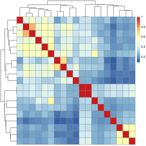
(a) Communication Services

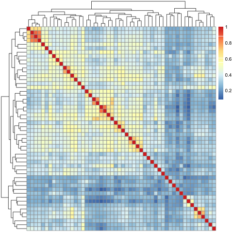
(b) Consumer Discretionary

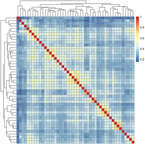
(c) Health Care

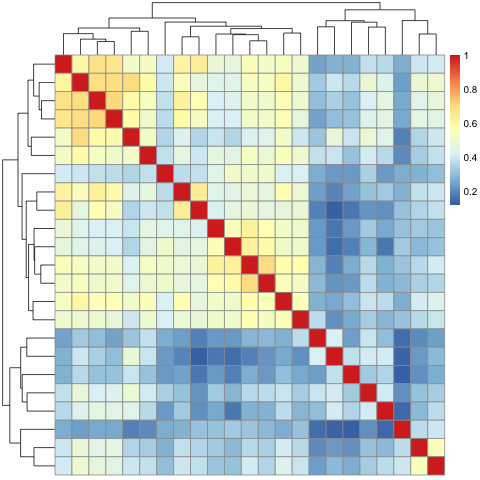
(d) Consumer Staples

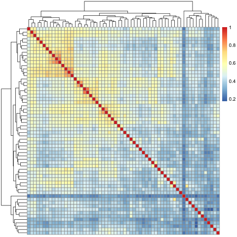
(e) Information Technology

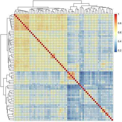
(f) Industrials

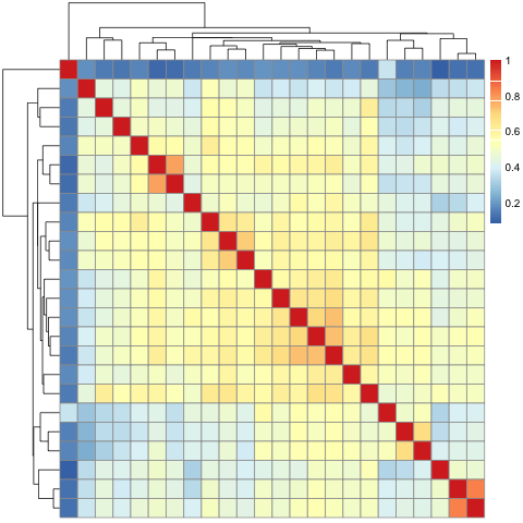
(g) Materials

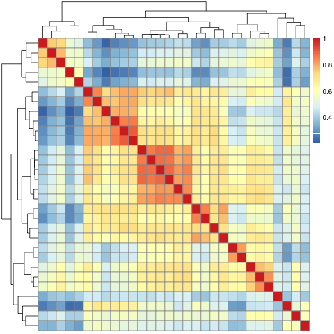
(h) Real Estate

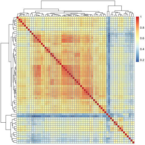
(i) Financials

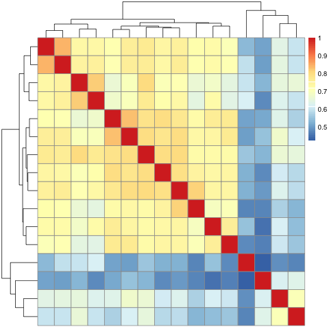
(j) Energy

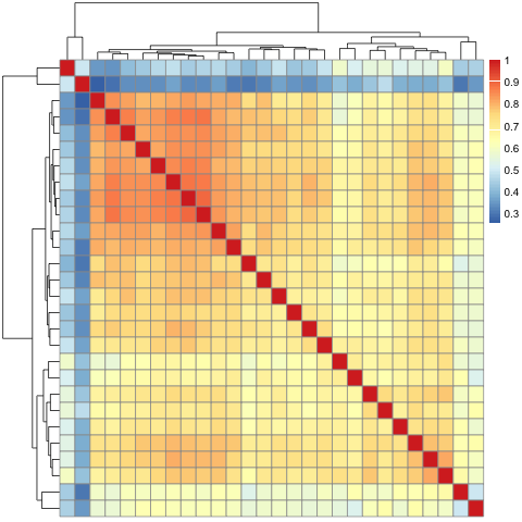
(k) Utilities

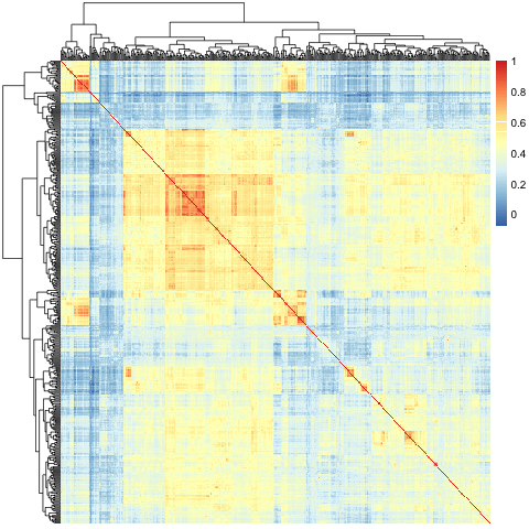
(l) The total

Figure 2: The correlation matrices of the stock returns of the 12 datasets of Table 1 and the total.

Although Figure 2 shows the various structures of $\mathbf{C}$ for the 12 datasets, $\lambda_{1}(\mathbf{C})/N$ predicts well the time average $\overline{\rho}$ of the time series of equi-correlation coefficients computed by GJR GARCH-DECO with much time. A regression analysis (Figure 3) for Table 1 shows:

$$\overline{\rho}\sim 0.98488\frac{\lambda_{1}(\mathbf{C})}{N}-0.07190\quad(\mbox{adjusted $R^{2}$ being 0.9916}).$$

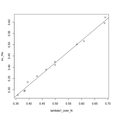
Figure 3: The regression analysis of $\overline{\rho}$ by $\lambda_{1}(\mathbf{C})/N$.

4 Phase transition of limiting distribution of largest eigenvalue

In our setting, all the correlation coefficients among $N$ variables being the positive constant $\rho$. It is, however, somehow unnatural in the limit $N\to\infty.$ We assume that

$$N>T$$

and the equi-correlation coefficient $\rho$ converges to 0 from above as $N\to\infty$.

For this setting with $N>T$, the consistency $\lambda_{1}(\mathbf{S})/N\to\rho$ of the largest eigenvalue $\lambda_{1}(\mathbf{S})$ and the asymptotic normality of $\lambda_{1}(\mathbf{S})$ for a nonnormal population follows from Yata & Aoshima (2009). Moreover, the limiting distribution of $\lambda_{1}(\mathbf{S})$ for an equi-correlated normal population seems to have a phase transition depending on the equi-correlation coefficient $\rho$, as the limiting distribution of the largest eigenvalue of $\mathbf{S}$ formed by a spiked population model does so with respect to the largest eigenvalue of the population covariance matrix (Baik et al., 2005).

4.1 Consistency and asymptotic normality of $\lambda_{1}(\mathbf{S})$ of nonnormal population

In (Yata & Aoshima, 2009), the consistency and the asymptotic normality of $\lambda_{1}(\mathbf{S})$ are proved without assuming the normality of the population.

Proposition 4.1.

Let a data matrix ${\mathbf{X}}\in{{\mathbb{R}}}^{N\times T}$ be $[\bm{X}_{1},\ldots,\bm{X}_{T}]$ where $\bm{X}_{t}$ $(1\leq t\leq T)$ are centered, i.i.d. and $N>T$. Suppose that the population covariance matrix ${\mathbf{\Sigma}}$ is $\mathbf{H}\operatorname{diag}(\lambda_{1},\ldots,\lambda_{N})\mathbf{H}^{\top}$ for some orthogonal matrix $\mathbf{H}$,

$$\lambda_{1}\geq\lambda_{2}\geq\cdots\geq\lambda_{N}\geq 0,$$

$$\lambda_{i}=c_{i}N^{\delta_{i}}\ (i=1,\ldots,m),\ \mbox{and}$$ (5)

$$\mbox{$\lambda_{j}$ are constants $(j=m+1,\ldots,N)$}.$$

Here $m$, $c_{i}(>0)$ and $\delta_{i}$ $(\delta_{1}\geq\cdots\geq\delta_{m}>0)$ are constants.

Let $\mathbf{Z}:=[\bm{Z}_{1},\ldots,\bm{Z}_{N}]:=\operatorname{diag}(\lambda_{1},\ldots,\lambda_{N})^{-1/2}\mathbf{H}^{\top}{\mathbf{X}}$. Assume that $\bm{Z}_{1},\ldots,\bm{Z}_{N}$ are independent, the fourth moments of the entries of $\mathbf{Z}$ are uniformly bounded, and no $\bm{Z}_{i}$ is $\bm{0}$. Moreover suppose

1. $N,T\to\infty$ for $i$ such that $\delta_{i}>1$; and

2. $N,T\to\infty$ and $N^{2-2\delta_{i}}/T\to 0$ for $i$ such that $\delta_{i}\in(0,\,1]$.

Then, we have

1. $\lambda_{1}(\mathbf{S})/\lambda_{1}=1+o_{p}(1)$. (Yata & Aoshima, 2009, Theorem 1)

2. Assume also that the largest $m$ eigenvalues of ${\mathbf{\Sigma}}$ are distinct and $\operatorname{Var}(z_{ij}^{2})=M_{i}\ (<\infty)$. Then, $\sqrt{T/M_{i}}(\lambda_{1}(\mathbf{S})/\lambda_{1}-1)\mathrel{\stackrel{{\scriptstyle D}}{{\to}}}\mathrm{N}(0,\,1)$. (Yata & Aoshima, 2009, Theorem 2)

The condition (ii) is relieved for (Yata & Aoshima, 2009, Theorem 2) if an independence condition is further assumed.

Proposition 4.2 ((Yata & Aoshima, 2009, Corollary 1)).

In the assertion (2) of Proposition 4.1, assume further that $z_{ij}$, $1\leq i\leq N(1\leq t\leq T)$ are independent. Then, it holds that $\lambda_{1}(\mathbf{S})/\lambda_{1}=1+o_{p}(1)$ if the condition (i) and

(iii)  $N,T\to\infty$ and $N^{1-2\delta_{i}}/T\to 0$ for $i$ such that $\delta_{i}\in(0,\,1]$.

By (3), ${\mathbf{\Sigma}}_{\rho}$ does not meet the condition (5). According to Kazuyoshi Yata, the conclusions of (Yata & Aoshima, 2009, Theorem 1) and (Yata & Aoshima, 2009, Theorem 2) indeed hold for ${\mathbf{\Sigma}}={\mathbf{\Sigma}}_{\rho}$. Therefore, we get the following:

Theorem 4.3.

Suppose that a population is possibly nonnormal, the population covariance matrix is ${\mathbf{\Sigma}}_{\rho}$ $(\rho>0)$, and $N,T\to\infty,{T/N\to Q}\in(0,\,\infty)$. Assume

1. the setting of (Yata & Aoshima, 2009, Theorem 1) and $\lim_{N\to\infty}N^{1/2}\rho=\infty$; or

2. the setting of (Yata & Aoshima, 2009, Corollary 1) and $\lim_{N\to\infty}N\rho=\infty$.

Then, we have ${\lambda_{1}(\mathbf{S})}/{N}\mathrel{\stackrel{{\scriptstyle P}}{{\to}}}\rho$ and the asymptotic normality of $\lambda_{1}(\mathbf{S})$.

4.2 Phase transition of limiting distribution of $\lambda_{1}(\mathbf{S})$ for normal population as to decay rate of equi-correlation coefficient

The limiting distribution of an appropriate scaling of a translation of the largest eigenvalue $\lambda_{1}(\mathbf{S})$ of a sample covariance matrix $\mathbf{S}$ is Tracy-Widom distribution if the equi-correlation coefficient $\rho$ is 0, by (Johnstone, 2001; Soshnikov, 2002), and a normal distribution if $\rho$ is a positive constant by Theorem 5.2. In view of Theorem 4.3 (2), we turn our attention to the case $\lim_{N\to\infty}N\rho<\infty$.

First, we recall (Baik et al., 2005, Theorem 1.1 and Corollary 1.1).

Proposition 4.4.

Assume $Q>1$ and the population is $\mathrm{N}_{N}(\bm{\mu},\,{\mathbf{\Sigma}})$, and $\lambda_{1}\geq\lambda_{2}\geq\lambda_{r}\geq\lambda_{r+1}=\cdots=\lambda_{N}=1$ be the eigenvalues of ${\mathbf{\Sigma}}$.

• Suppose $0\leq k\leq r$, $\lambda_{1}=\cdots=\lambda_{k}=1+1/\sqrt{Q}$, and $\set{\lambda_{k+1},\ldots,\lambda_{r}}\subset(0,\,1+1/\sqrt{Q})$. Then,

  $$\lambda_{1}(\mathbf{S})\mathrel{\stackrel{{\scriptstyle P}}{{\to}}}{(1+\sqrt{1/Q})^{2}},\ \mbox{and}$$

  $$\operatorname{P}\left(\left(\lambda_{1}(\mathbf{S})-{(1+\sqrt{1/Q})^{2}}\right)\cdot\frac{\sqrt{Q}}{(1+\sqrt{Q})^{4/3}}T^{2/3}\leq x\right)\to F_{\mathrm{TW},k}(x),$$ (6)

  where $F_{\mathrm{TW},k}(x)$ is the distribution function of a generalization of the Tracy-Widom distribution (Baik et al., 2005, Definition 1.1).

• Suppose $1\leq k\leq r$, $\lambda_{1}=\cdots=\lambda_{k}>1+1/\sqrt{Q}$, and $\set{\lambda_{k+1},\ldots,\lambda_{r}}\subset(0,\lambda_{1})$. Then,

  $$\lambda_{1}(\mathbf{S})\stackrel{{\scriptstyle P}}{{\to}}\lambda_{1}+\frac{Q^{-1}\lambda_{1}}{\lambda_{1}-1},\ \mbox{and}$$

  $$\operatorname{P}\left(\left(\lambda_{1}(\mathbf{S})-\left(\lambda_{1}+\frac{Q^{-1}\lambda_{1}}{\lambda_{1}-1}\right)\right)\cdot\frac{\sqrt{T}}{\sqrt{\lambda_{1}^{2}-Q^{-1}\lambda_{1}^{2}/(\lambda_{1}-1)^{2}}}\leq x\right)\to F_{\mathrm{G},k}(x),$$ (7)

  where $F_{\mathrm{G},k}(x)$ is the distribution function of a generalization of the Gaussian distribution (Baik et al., 2005, Definition 1.2).

This proposition suggests the following phase transition: For a normal population, if $\lim_{N\to\infty}N\rho>1/\sqrt{Q}$, then the largest eigenvalue $\lambda_{1}(\mathbf{S})$ satisfies the asymptotic normality in a sense of (6), and if $\lim_{N\to\infty}N\rho<1/\sqrt{Q}$, then an appropriate scaling of a translation of $\lambda_{1}(\mathbf{S})$ converges to the Tracy-Widom distribution $G_{1}$ in a sense of (7). This holds for $\lim_{N\to\infty}N\rho=\infty$ by Theorem 4.3.

The detail of this phase transition will be studied elsewhere.

5 Proof of Theorem 1.3

We also consider centered (noncentered, resp.) variant of the sample covariance matrix $\mathbf{S}\in{{\mathbb{R}}}^{N\times N}$ (the sample correlation matrix $\mathbf{C}\in{{\mathbb{R}}}^{N\times N}$, resp.):

Definition 5.1.

Let ${\mathbf{\tilde{Y}}}$ be $\operatorname{diag}\left(\lVert\bm{x}_{1}\rVert^{-1},\ldots,\lVert\bm{x}_{N}\rVert^{-1}\right){\mathbf{X}}\in{{\mathbb{R}}}^{N\times T}$. Define the following three matrices:

$${\mathbf{\tilde{C}}}\ \ :={\mathbf{\tilde{Y}}}{\mathbf{\tilde{Y}}}^{\top}\in{{\mathbb{R}}}^{N\times N} \mbox{(\emph{noncentered sample correlation matrix})},$$

$$\mathbf{E}\ \ :=T^{-1/2}({\mathbf{X}}-\overline{\mathbf{X}})\in{{\mathbb{R}}}^{N\times T},$$

$$\mathbf{S}^{\circ}\ :=\mathbf{E}\mathbf{E}^{\top}\in{{\mathbb{R}}}^{N\times N} \mbox{(\emph{centered sample covariance matrix})}.$$

To prove Theorem 1.3 (1), we will prove:

Theorem 5.2.

Assume that $\bm{X}_{1},\ldots,\bm{X}_{T}\mathrel{\stackrel{{\scriptstyle\mbox{\emph{i.\@i.\@d.\@}}}}{{\sim}}}\mathrm{N}_{N}(\bm{\mu},\,\bm{\Delta}{\mathbf{\Sigma}}_{\rho}\bm{\Delta})$, $\bm{\mu}\in{{\mathbb{R}}}^{N}$ is deterministic, $\bm{\Delta}$ is deterministic, nonsingular diagonal, and $\rho\in[0,\,1)$ is deterministic. Suppose $({\mathbf{P}}=\mathbf{S}$, $\bm{\mu}=\bm{0}$, $\bm{\Delta}=\mathbf{I})$, $({\mathbf{P}}=\mathbf{S}^{\circ}$, $\bm{\Delta}=\mathbf{I})$, $({\mathbf{P}}={\mathbf{\tilde{C}}}$, $\bm{\mu}=\bm{0})$, or ${\mathbf{P}}=\mathbf{C}$. Then, ${\lambda_{1}({\mathbf{P}})}/{N}\mathrel{\stackrel{{\scriptstyle a.s.}}{{\to}}}\rho$.

Proof 5.3.

First consider the case where ${\mathbf{P}}=\mathbf{S}$, $\bm{\mu}=\bm{0}$, and $\bm{\Delta}=\mathbf{I}$. Suppose $\rho=0$. Then, all the entries of ${\mathbf{X}}$ are standard normal, so they are independent and $\operatorname{E}|x_{11}|^{4}<\infty$. Thus,

$$\lim_{N,T\to\infty,{T/N\to Q}}\lambda_{1}(\mathbf{S})=b_{Q}\quad(a.s.)$$

by (Bai & Yin, 1993, Theorem 2). Hence, Theorem 5.2 (1) holds for this case when $\rho=0$.

Then, we prove $\lambda_{1}(\mathbf{S})/N\mathrel{\stackrel{{\scriptstyle a.s.}}{{\to}}}\rho$ for $\rho>0$. For this, we recall (Merlevède et al., 2019, Proposition 2.1), which is due to (Ledoit & Wolf, 2018, Proposition 7.3) and (Cai et al., 2017, Theorem 2.1) according to Merlevède et al. (2019). Following (Van der Vaart, 2000, p. 8), we say a sequence $(F_{N})_{N}$ of distribution functions is tight on ${{\mathbb{R}}}^{+}$, if for every $\epsilon\in(0,\,1]$, there is a constant $M\geq 0$ such that

$$\sup_{N}F_{N}(M)>1-\epsilon.$$

Proposition 5.4 (Merlevède et al. (2019, Proposition 2.1)).

Assume

1. $\mathbf{S}=T^{-1}{{\mathbf{\Sigma}}}^{1/2}{\mathbf{G}}{\mathbf{G}}^{\top}{{\mathbf{\Sigma}}}^{1/2}\in{{\mathbb{R}}}^{N\times N}$, the entries of ${\mathbf{G}}\in{{\mathbb{R}}}^{N\times T}$ are independent, standard normal, and ${{\mathbf{\Sigma}}}\in{{\mathbb{R}}}^{N\times N}$ is positive definite, symmetric, and deterministic.

2. A sequence $\left(F^{{{\mathbf{\Sigma}}}}\right)_{N}$ of empirical spectral distributions is tight on ${{\mathbb{R}}}^{+}$, and $\lim_{N\to\infty}\lambda_{1}({{\mathbf{\Sigma}}})=\infty$.

3. ${{N,T\to\infty,\ {T/N\to Q}}}\in(0,\infty)$.

Then, ${\lambda_{1}(\mathbf{S})}/{\lambda_{1}({{\mathbf{\Sigma}}})}\mathrel{\stackrel{{\scriptstyle a.s.}}{{\to}}}1.$

The sequence $\left(F^{{\mathbf{\Sigma}}_{\rho}}\right)_{N}$ of the empirical spectral distribution function of ${\mathbf{\Sigma}}_{\rho}\in{{\mathbb{R}}}^{N\times N}$ is a tight sequence on ${{\mathbb{R}}}^{+}$. To see it, consider $\epsilon\in(0,\,1]$ and $M=(\epsilon^{-1}-1)\rho+1>0$. For every integer $N>M$, $\lambda_{1}({\mathbf{\Sigma}}_{\rho})>M$, so $F^{{\mathbf{\Sigma}}_{\rho}}(M)=1$. Hence, $\sup_{N}F^{{\mathbf{\Sigma}}_{\rho}}(M)\geq 1-\epsilon$. Therefore, we have the tightness of the sequence.

Then, by Proposition 5.4 with ${{\mathbf{\Sigma}}}:={\mathbf{\Sigma}}_{\rho}\in{{\mathbb{R}}}^{N\times N}$, ${\lambda_{1}(\mathbf{S})}\big{/}\left((N-1)\rho+1\right)={\lambda_{1}(\mathbf{S})}\big{/}{\lambda_{1}({\mathbf{\Sigma}}_{\rho})}\mathrel{\stackrel{{\scriptstyle a.s.}}{{\to}}}1.$ Thus, we have established $\lambda_{1}(\mathbf{S})/N\mathrel{\stackrel{{\scriptstyle a.s.}}{{\to}}}\rho$ for every $\rho\geq 0$.

Now, we consider the case where ${\mathbf{P}}=\mathbf{S}^{\circ}$ and $\bm{\Delta}=\mathbf{I}$. We will derive ${\lambda_{1}(\mathbf{S}^{\circ})}/{N}\mathrel{\stackrel{{\scriptstyle a.s.}}{{\to}}}\rho$ for every $\rho\geq 0$, by using the following:

Proposition 5.5 (Bai & Yin (1993, Lemma 2)).

Let $\set{y_{kj}\colon\,k,j\geq 1}$ be a double array of i.i.d. random variables and let $\alpha>{1}/{2}$, $\beta\geq 0$ and $M>0$ be constants. Then,

$$\max_{j\leq MT^{\beta}}\left|\sum_{k=1}^{T}\frac{y_{kj}-m}{T^{\alpha}}\right|\mathrel{\stackrel{{\scriptstyle a.s.}}{{\to}}}0\quad(T\to\infty)$$

$$\iff \operatorname{E}|y_{11}|^{\frac{1+\beta}{\alpha}}<\infty\;\&\;m=\begin{cases}\displaystyle\operatorname{E}y_{11},&(\alpha\leq 1),\\ \displaystyle\text{\rm any},&(\alpha>1).\end{cases}$$

Proposition 5.5 is also used to prove Theorem 2.3 in Section 7.

The centered sample covariance matrix $\mathbf{S}^{\circ}$ is invariant with respect to the shifting of variables. By this invariance, we can assume $\bm{\mu}=\bm{0}.$ It suffices to assure

$$\lim_{{\begin{subarray}{c}N,T\to\infty\\ {T/N\to Q}\end{subarray}}}\left|\sqrt{\frac{\lambda_{1}(\mathbf{S}^{\circ})}{N}}-\sqrt{\frac{\lambda_{1}(\mathbf{S})}{N}}\right|=0\quad(a.s.).$$

By the triangle inequality for the spectral norm,

$$\left|\sqrt{\lambda_{1}(\mathbf{S}^{\circ})}-\sqrt{\lambda_{1}(\mathbf{S})}\right|=\left|\vvvert T^{-1/2}({\mathbf{X}}-\overline{\mathbf{X}})\vvvert-\vvvert T^{-1/2}{\mathbf{X}}\vvvert\right|\leq\vvvert T^{-1/2}\overline{\mathbf{X}}\vvvert.$$ (8)

The last term $\vvvert T^{-1/2}\overline{\mathbf{X}}\vvvert$ is $\sqrt{\sum_{i=1}^{N}\overline{x}_{i}^{2}}$ (a.s.). To see it, note that the $it$-entry of $T^{-1}\overline{\mathbf{X}}\,\overline{\mathbf{X}}^{\top}$ is $T^{-1}\sum_{k=1}^{T}\overline{x}_{i}\overline{x}_{t}=\overline{x}_{i}\overline{x}_{t}$. Therefore, $[\overline{x}_{1},\ldots,\overline{x}_{N}]^{\top}$ is an eigenvector of $T^{-1}\overline{\mathbf{X}}\,\overline{\mathbf{X}}^{\top}$, corresponding to an eigenvalue $\sum_{i=1}^{N}\overline{x}_{i}^{2}$. Clearly, $\operatorname{rank}\overline{\mathbf{X}}\leq 1$ and almost surely $\operatorname{rank}\overline{\mathbf{X}}=1$. Thus, it is also the case for $\operatorname{rank}T^{-1}\overline{\mathbf{X}}\,\overline{\mathbf{X}}^{\top}$. Considering the eigenvalue $\sum_{i=1}^{N}\overline{x}_{i}^{2}$ of $T^{-1}\overline{\mathbf{X}}\,\overline{\mathbf{X}}^{\top}$ is positive almost surely, the other $N-1$ eigenvalues are 0 almost surely.

By dividing (8) with $\sqrt{N}$, it holds almost surely that

$$\left|\sqrt{\frac{\lambda_{1}(\mathbf{S}^{\circ})}{N}}-\sqrt{\frac{\lambda_{1}(\mathbf{S})}{N}}\right|\leq\sqrt{\sum_{i=1}^{N}\frac{\overline{x}_{i}^{2}}{N}}\leq\sqrt{\max_{1\leq i\leq N}\left({\sum_{t=1}^{T}}\frac{x_{it}}{T}\right)^{2}}=\max_{1\leq i\leq N}\left|{\sum_{t=1}^{T}}\frac{x_{it}}{T}\right|.$$ (9)

By $\bm{\Delta}=\mathbf{I}$ and $\bm{\mu}=\bm{0}$, $x_{it}$ $(i,t\geq 1)$ are standard normal random variables equi-correlated with $\rho\in[0,1)$. By decomposition (4), there are independent standard normal random variables ${{f}}_{t},e_{it}$ $(i,t\geq 1)$ such that $x_{it}=\sqrt{\rho}{{f}}_{t}+\sqrt{1-\rho}e_{it}$. By the triangle inequality,

$$\max_{1\leq i\leq N}\left|{\sum_{t=1}^{T}}\frac{x_{it}}{T}\right|\leq\left|{\sum_{t=1}^{T}}\frac{\sqrt{\rho}{{f}}_{t}}{T}\right|+\max_{1\leq i\leq N}\left|{\sum_{t=1}^{T}}\frac{\sqrt{1-\rho}e_{it}}{T}\right|.$$

The first term of the right side tends to 0 in $T\to\infty$ almost surely, by the law of large numbers. The second term of the right side tends to 0 in $N,T\to\infty,\ {T/N\to Q}$ almost surely, by Proposition 5.5 with $\alpha=\beta=1$ and $M=Q$. Thus,

$$\max_{1\leq i\leq N}|\overline{x}_{i}|=\max_{1\leq i\leq N}\left|{\sum_{t=1}^{T}}\frac{x_{it}}{T}\right|{\stackrel{{\scriptstyle a.s.}}{{\to}}}0\quad({{N,T\to\infty,\ {T/N\to Q}}}).$$ (10)

Hence, $\eqref{qq}\mathrel{\stackrel{{\scriptstyle a.s.}}{{\to}}}0$. Since we have already established ${\lambda_{1}(\mathbf{S})}/{N}\mathrel{\stackrel{{\scriptstyle a.s.}}{{\to}}}\rho$ for every $\rho\geq 0$, we then derived ${\lambda_{1}(\mathbf{S}^{\circ})}/{N}\mathrel{\stackrel{{\scriptstyle a.s.}}{{\to}}}\rho$ for every $\rho\geq 0$.

We consider the case ${\mathbf{P}}={\mathbf{\tilde{C}}}$ and $\bm{\mu}=\bm{0}$. Because the noncentered sample correlation matrix ${\mathbf{\tilde{C}}}$ is invariant under the scaling, we can assume

$$\bm{\Delta}=\mathbf{I}.$$

From ${\lambda_{1}(\mathbf{S})}/{N}\mathrel{\stackrel{{\scriptstyle a.s.}}{{\to}}}\rho$ of Theorem 5.2, we will guarantee

$$\lim_{{\begin{subarray}{c}N,T\to\infty\\ {T/N\to Q}\end{subarray}}}\left|\sqrt{\frac{\lambda_{1}({\mathbf{\tilde{C}}})}{N}}-\sqrt{\frac{\lambda_{1}(\mathbf{S})}{N}}\right|=0\quad(a.s.).$$ (11)

For a diagonal matrix

$${{\tilde{\mathbf{D}}}}=\operatorname{diag}\left(\frac{\sqrt{T}}{\lVert{\bm{x}_{1}}\rVert},\ldots,\frac{\sqrt{T}}{\lVert{\bm{x}_{N}}\rVert}\right),\quad\lVert\bm{x}_{i}\rVert=\sqrt{{\sum_{t=1}^{T}}x_{it}^{2}}$$

we have ${\mathbf{\tilde{Y}}}=T^{-1/2}{{\tilde{\mathbf{D}}}}{\mathbf{X}}$.

Recall that the spectral norm of a matrix $\mathbf{M}\in{{\mathbb{R}}}^{m\times n}$ is

$$\vvvert\mathbf{M}\vvvert=\sup_{\bm{X}\in{{\mathbb{R}}}^{n},\lVert\bm{X}\rVert=1}\lVert\mathbf{M}\bm{X}\rVert.$$

Note $\vvvert\mathbf{M}\vvvert=\sqrt{\lambda_{1}(\mathbf{M}^{\top}\mathbf{M})}$. By the triangle inequality of the spectral norm and that $\vvvert\mathbf{M}_{1}\mathbf{M}_{2}\vvvert\leq\vvvert\mathbf{M}_{1}\vvvert\vvvert\mathbf{M}_{2}\vvvert$ for every $\mathbf{M}_{1}\in{{\mathbb{R}}}^{N\times N}$ and $\mathbf{M}_{2}\in{{\mathbb{R}}}^{N\times T}$,

$$\left|\sqrt{\frac{\lambda_{1}({\mathbf{\tilde{C}}})}{N}}-\sqrt{\frac{\lambda_{1}(\mathbf{S})}{N}}\right|\leq\left\vvvert\frac{1}{\sqrt{N}}{\mathbf{\tilde{Y}}}-\frac{1}{\sqrt{NT}}{\mathbf{X}}\right\vvvert=\vvvert(NT)^{-1/2}({{\tilde{\mathbf{D}}}}-\mathbf{I}){\mathbf{X}}\vvvert$$ (12)

$$\leq\vvvert{{\tilde{\mathbf{D}}}}-\mathbf{I}\vvvert\cdot\vvvert(NT)^{-1/2}{\mathbf{X}}\vvvert=\max_{{1\leq i\leq N}}\left|\frac{T^{1/2}}{\lVert\bm{x}_{i}\rVert}-1\right|\cdot\sqrt{\frac{\lambda_{1}(\mathbf{S})}{N}}.$$ (13)

Since we established ${\lambda_{1}(\mathbf{S})}/{N}\mathrel{\stackrel{{\scriptstyle a.s.}}{{\to}}}\rho$ from $\bm{\Delta}=\mathbf{I}$ and $\bm{\mu}=\bm{0}$, it suffices to verify

$$\lim_{{\begin{subarray}{c}N,T\to\infty\\ {T/N\to Q}\end{subarray}}}\max_{{{1\leq i\leq N}}}\left|\frac{\sqrt{T}}{\lVert\bm{x}_{i}\rVert}-1\right|=0\quad(a.s.).$$ (14)

By decomposition (4), there are independent standard normal random variables ${{f}}_{t},e_{it}$ $(i,t\geq 1)$ such that $x_{it}=\sqrt{\rho}{{f}}_{t}+\sqrt{1-\rho}e_{it}$. Hence,

$${\sum_{t=1}^{T}}\frac{x_{it}^{2}}{T}=\rho{\sum_{t=1}^{T}}\frac{{{f}}_{t}^{2}}{T}+2\sqrt{\rho(1-\rho)}{\sum_{t=1}^{T}}\frac{{{f}}_{t}e_{it}}{T}+(1-\rho){\sum_{t=1}^{T}}\frac{e_{it}^{2}}{T}.$$

Then

$$\max_{{{1\leq i\leq N}}}\left|\frac{\lVert\bm{x}_{i}\rVert^{2}}{T}-1\right|=\max_{{{1\leq i\leq N}}}\left|{\sum_{t=1}^{T}}\frac{x_{it}^{2}}{T}-1\right|$$

$$\leq \rho\max_{{{1\leq i\leq N}}}\left|{\sum_{t=1}^{T}}\frac{{{f}}_{t}^{2}}{T}-1\right|+2\sqrt{\rho(1-\rho)}\max_{{1\leq i\leq N}}\left|{\sum_{t=1}^{T}}\frac{{{f}}_{t}e_{it}}{T}\right|+(1-\rho)\max_{{{1\leq i\leq N}}}\left|{\sum_{t=1}^{T}}\frac{e_{it}^{2}}{T}-1\right|.$$

The right side converges almost surely to 0 by Proposition 5.5, because ${{f}}_{t}^{2}$ $(t\geq 1)$ are i.i.d. of unit mean, ${{f}}_{t}e_{it}$ $(i,t\geq 1)$ are centered i.i.d., and $e_{it}^{2}$ $(i,t\geq 1)$ are i.i.d. of unit mean. Hence,

$$\lim_{{\begin{subarray}{c}N,T\to\infty\\ {T/N\to Q}\end{subarray}}}\max_{{{1\leq i\leq N}}}\left|\frac{\lVert\bm{x}_{i}\rVert^{2}}{T}-1\right|=0\quad(a.s.),$$ (15)

from which $\left|{\lVert\bm{x}_{i}\rVert^{2}}/{T}-1\right|>\left|{\lVert\bm{x}_{i}\rVert}/{\sqrt{T}}-1\right|$ implies

$$\lim_{{\begin{subarray}{c}N,T\to\infty\\ {T/N\to Q}\end{subarray}}}\max_{{{1\leq i\leq N}}}\left|\frac{\lVert\bm{x}_{i}\rVert}{\sqrt{T}}-1\right|=0\quad(a.s.).$$ (16)

Suppose $\max_{1\leq i\leq N}\left|{\lVert\bm{x}_{i}\rVert}/{\sqrt{T}}-1\right|<\epsilon$ for sufficiently small $\epsilon>0$. Then, for all $i$ $(1\leq i\leq N)$, $1-\epsilon<{\lVert\bm{x}_{i}\rVert}/\sqrt{T}<1+\epsilon$, which implies $(1+\epsilon)^{-1}-1<\sqrt{T}/{\lVert\bm{x}_{i}\rVert}-1<(1-\epsilon)^{-1}-1$. Hence, for all $i$ $(1\leq i\leq N)$, $\left|\sqrt{T}/{\lVert\bm{x}_{i}\rVert}-1\right|<\max((1-\epsilon)^{-1}-1,\ \left|(1+\epsilon)^{-1}-1\right|)<\epsilon+\epsilon^{2}+\epsilon^{3}+\cdots<2\epsilon$, because $0<\epsilon\ll 1$. Thus, $\max_{1\leq i\leq N}\left|\sqrt{T}/{\lVert\bm{x}_{i}\rVert}-1\right|<2\epsilon$. Therefore, from (16), (14) follows.

Thus, (11) is guaranteed. Therefore, ${\lambda_{1}({\mathbf{\tilde{C}}})}/{N}\mathrel{\stackrel{{\scriptstyle a.s.}}{{\to}}}\rho$ follows because the assumption $\bm{\mu}=\bm{0}$ implies ${\lambda_{1}(\mathbf{S})}/{N}\mathrel{\stackrel{{\scriptstyle a.s.}}{{\to}}}\rho$.

At last, we will demonstrate ${\lambda_{1}(\mathbf{C})}/{N}\mathrel{\stackrel{{\scriptstyle a.s.}}{{\to}}}\rho$ of Theorem 5.2. Because the sample correlation matrix $\mathbf{C}$ is invariant under the shifting and scaling, we can assume $\bm{\Delta}=\mathbf{I}$ and $\bm{\mu}=\bm{0}$. For $\mathbf{C}={\mathbf{Y}}{\mathbf{Y}}^{\top}$, we have ${\mathbf{Y}}=T^{-1/2}\mathbf{D}({\mathbf{X}}-\overline{\mathbf{X}})$ where

$$\mathbf{D}=\operatorname{diag}\left({\sqrt{T}}/{\lVert{\bm{x}_{1}-{\overline{\bm{x}}}_{1}}\rVert},\ldots,{\sqrt{T}}/{\lVert{\bm{x}_{N}-{\overline{\bm{x}}}_{N}}\rVert}\right).$$

Recall $\mathbf{S}^{\circ}=T^{-1}({\mathbf{X}}-\overline{\mathbf{X}})({\mathbf{X}}-\overline{\mathbf{X}})^{\top}$. By the same arguments as in (13),

$$\left|\sqrt{\frac{\lambda_{1}(\mathbf{C})}{N}}-\sqrt{\frac{\lambda_{1}(\mathbf{S}^{\circ})}{N}}\right|\leq\max_{{1\leq i\leq N}}\left|\frac{\sqrt{T}}{\lVert{\bm{x}_{i}-{\overline{\bm{x}}}_{i}}\rVert}-1\right|\cdot\sqrt{\frac{\lambda_{1}(\mathbf{S}^{\circ})}{N}}.$$

Because ${\lambda_{1}(\mathbf{S}^{\circ})}/{N}\mathrel{\stackrel{{\scriptstyle a.s.}}{{\to}}}\rho$ follows from $\bm{\Delta}=\mathbf{I}$ we assumed, it suffices to show

$$\lim_{{\begin{subarray}{c}N,T\to\infty\\ {T/N\to Q}\end{subarray}}}\max_{{1\leq i\leq N}}\left|\frac{\sqrt{T}}{\lVert{\bm{x}_{i}-{\overline{\bm{x}}}_{i}}\rVert}-1\right|=0\quad(a.s.).$$ (17)

By $\lVert\bm{x}_{i}-{\overline{\bm{x}}}_{i}\rVert^{2}=\lVert\bm{x}_{i}\rVert^{2}-T\left|\overline{x}_{i}\right|^{2}$,

$$\max_{{{1\leq i\leq N}}}\left|\frac{\lVert\bm{x}_{i}-{\overline{\bm{x}}}_{i}\rVert^{2}}{T}-1\right|\leq\max_{{{1\leq i\leq N}}}\left|\frac{\lVert\bm{x}_{i}\rVert^{2}}{T}-1\right|+\max_{{{1\leq i\leq N}}}\left|\overline{x}_{i}\right|^{2}.$$

The first (second, resp.) term of the right side converges almost surely to 0, by (15) ((10), resp.). In a similar way as above, (17) is shown. Therefore, ${\lambda_{1}(\mathbf{C})}/{N}\mathrel{\stackrel{{\scriptstyle a.s.}}{{\to}}}\rho$ for every $\rho\geq 0$. This completes the proof of Theorem 5.2.

To prove Theorem 1.3 (2), we employ:

Proposition 5.6 (Merlevède et al. (2019, Theorem 2.2)).

Assume the three assumptions of Proposition 5.4. From a spectral gap condition on ${{\mathbf{\Sigma}}}$:

$$\limsup_{{\begin{subarray}{c}N,T\to\infty\\ {T/N\to Q}\end{subarray}}}\frac{\lambda_{2}({{\mathbf{\Sigma}}})}{\lambda_{1}({{\mathbf{\Sigma}}})}<1,$$ (18)

it follows that

$$\sqrt{T}\left(\frac{\lambda_{1}(\mathbf{S})}{\lambda_{1}({{\mathbf{\Sigma}}})}-1-\frac{1}{T}\sum_{k=2}^{N}\frac{\lambda_{k}({{\mathbf{\Sigma}}})}{\lambda_{1}({\mathbf{\Sigma}})-\lambda_{k}({\mathbf{\Sigma}})}\right)\mathrel{\stackrel{{\scriptstyle D}}{{\to}}}\mathrm{N}(0,\ 2).$$

The spectral gap condition (18) holds for ${\mathbf{\Sigma}}={\mathbf{\Sigma}}_{\rho}$ with $\rho>0$, because (3) implies

$$\limsup_{{\begin{subarray}{c}N,T\to\infty\\ {T/N\to Q}\end{subarray}}}\frac{\lambda_{2}({\mathbf{\Sigma}})}{\lambda_{1}({{\mathbf{\Sigma}}})}=\limsup_{{\begin{subarray}{c}N,T\to\infty\\ {T/N\to Q}\end{subarray}}}\frac{1-\rho}{(N-1)\rho+1}=0.$$

Then, ${T}^{-1}\sum_{k=2}^{N}{\lambda_{k}({{\mathbf{\Sigma}}})}/{\left(\lambda_{1}({{\mathbf{\Sigma}}})-\lambda_{k}({{\mathbf{\Sigma}}})\right)}={{(N-1)(1-\rho)}/{(NT\rho)}}$. This completes the proof of Theorem 1.3 (2).

6 Proof of Corollary 1.4

From Proposition 1.2, $F^{\mathbf{C}}(x)$ converges to $\mathrm{MP}_{Q,\,1-\rho}(x)$ almost surely for every $x\neq 0$. It suffices to prove that $\mathrm{MP}_{T/N,\,1-\lambda_{1}(\mathbf{C})/N}(x)$ converges almost surely to $\mathrm{MP}_{Q,\,1-\rho}(x)$ for any $x\neq 0$. By Theorem 1.3, $\lambda_{1}(\mathbf{C})/N\mathrel{\stackrel{{\scriptstyle a.s.}}{{\to}}}\rho$, so $x/(1-\lambda_{1}(\mathbf{C})/N))\mathrel{\stackrel{{\scriptstyle a.s.}}{{\to}}}x/(1-\rho)>0$. The distribution function $\mathrm{MP}_{Q}(t)$ of a Marčenko-Pastur distribution is continuous with respect to $t>0$. Thus,

$$\lim_{{\begin{subarray}{c}N,T\to\infty\\ {T/N\to Q}\end{subarray}}}\left|\mathrm{MP}_{T/N}\left(\frac{x}{1-\lambda_{1}(\mathbf{C})/N}\right)-\mathrm{MP}_{T/N}\left(\frac{x}{1-\rho}\right)\right|=0\quad(a.s.).$$ (19)

On the other hand, $\mathrm{MP}_{Q}(t)$ is continuous with respect to $Q\in(0,\infty)$ for each $t>0$, in view of the density function (1). Therefore,

$$\lim_{{\begin{subarray}{c}N,T\to\infty\\ {T/N\to Q}\end{subarray}}}\left|\mathrm{MP}_{T/N}\left(\frac{x}{1-\rho}\right)-\mathrm{MP}_{Q}\left(\frac{x}{1-\rho}\right)\right|=0\quad(a.s).$$

By this, (19), and the triangle inequality,

$$\lim_{{\begin{subarray}{c}N,T\to\infty\\ {T/N\to Q}\end{subarray}}}\left|\mathrm{MP}_{T/N}\left(\frac{x}{1-\lambda_{1}(\mathbf{C})/N}\right)-\mathrm{MP}_{Q}\left(\frac{x}{1-\rho}\right)\right|=0\quad(a.s.).$$

7 Proof of Theorem 2.3

7.1 LSD of sample covariance matrix generated from factor model

In this subsection, we provide the LSD of the sample covariance matrix $\mathbf{S}$ generated from a factor model (Definition 2.1) in $N,T\to\infty,{T/N\to Q}$ with Assumption 2. Let $F_{1}$ and $F_{2}$ be distribution functions. The Lévy distance between $F_{1}$ and $F_{2}$ is denoted by $\operatorname{d_{L}}(F_{1},F_{2})$. For the definition, see (Huber & Ronchetti, 2009, Definition 2.7). By (Huber & Ronchetti, 2009, Theorem 2.9),

Proposition 7.1.

For every sequence $(F_{n})_{n}$ of distribution functions, and every distribution function $F$, $F_{n}$ converges weakly to $F$ if and only if $\operatorname{d_{L}}(F_{n},F)\to 0$.

By Huber & Ronchetti (2009, p. 36), the Kolmogorov distance between two $F_{1}$ and $F_{2}$ is defined as $\operatorname{d_{K}}(F_{1},F_{2})=\sup_{x\in{{\mathbb{R}}}}\left|F_{1}(x)-F_{2}(x)\right|$, and satisfies

$$\operatorname{d_{L}}(F_{1},F_{2})\leq\operatorname{d_{K}}(F_{1},F_{2}).$$ (20)

Proposition 7.2 (Bai (1999, Lemma 2.6, the rank inequality)).

$$\operatorname{d_{K}}\left(F^{{\mathbf{A}}{\mathbf{A}}^{\top}},F^{\mathbf{B}\mathbf{B}^{\top}}\right)\leq\frac{1}{N}\;\operatorname{rank}({\mathbf{A}}-\mathbf{B}),\qquad\left({\mathbf{A}},\mathbf{B}\in{{\mathbb{R}}}^{N\times T}\right).$$

Theorem 7.3 (Scaling).

Given a factor model. Suppose ${{N,T\to\infty,\ {T/N\to Q}}}\in(0,\,\infty)$ and Assumption 2. Then, the following two hold almost surely:

1. $F^{\mathbf{S}}$ converges weakly almost surely to $\mathrm{MP}_{Q,\sigma_{\infty}^{2}(1-\rho)}$, if $\mu_{i}=0$ $(1\leq i\leq N)$.

2. $F^{\mathbf{E}\mathbf{E}^{\top}}$ converges weakly almost surely to $\mathrm{MP}_{Q,\sigma_{\infty}^{2}(1-\rho)}$.

Proof 7.4.

By Definition 2.1, the data matrix is written as

$${\mathbf{X}}={\sum_{k=1}^{K}}\left[\ell_{ik}f_{tk}\right]_{it}+\bm{\Psi},\quad\bm{\Psi}:=[e_{it}]_{it}\in{{\mathbb{R}}}^{N\times T}.$$ (21)

By Assumption 2 and Proposition 1.1 (1), the ESD of $T^{-1}\bm{\Psi}\bm{\Psi}^{\top}$ converges weakly to $\mathrm{MP}_{Q,\psi_{1}}$ almost surely. Then, Proposition 7.1 implies

$$\lim_{{\begin{subarray}{c}N,T\to\infty\\ {T/N\to Q}\end{subarray}}}\operatorname{d_{L}}\left(F^{{T}^{-1}\bm{\Psi}\bm{\Psi}^{\top}},\,\mathrm{MP}_{Q,\psi_{1}}\right)=0\quad(a.s.)$$ (22)

where $\psi_{1}=\sigma_{\infty}^{2}(1-\rho)$ by Assumption 2. Recall $\mathbf{S}=T^{-1}{\mathbf{X}}{\mathbf{X}}^{\top}$. Thus, by (20), Proposition 7.2, (21), and $\operatorname{rank}[\ell_{ik}f_{tk}]_{it}\leq 1$ $(1\leq k\leq K)$, it holds almost surely that

$$\operatorname{d_{L}}\left(F^{\mathbf{S}},\ F^{{T}^{-1}\bm{\Psi}\bm{\Psi}^{\top}}\right)\leq\operatorname{d_{K}}\left(F^{\mathbf{S}},\ F^{{T}^{-1}\bm{\Psi}\bm{\Psi}^{\top}}\right)\leq\frac{1}{N}\operatorname{rank}\left(\frac{1}{\sqrt{T}}{\mathbf{X}}-\frac{1}{\sqrt{T}}\bm{\Psi}\right)$$

$$=\frac{1}{N}\operatorname{rank}\left(\frac{1}{\sqrt{T}}{\sum_{k=1}^{K}}\left[\ell_{ik}f_{tk}\right]_{it}\right)\leq\frac{1}{N}{\sum_{k=1}^{K}}\operatorname{rank}\left(\left[\ell_{ik}f_{tk}\right]_{it}\right)\leq\frac{K}{N}\to 0\qquad(N\to\infty).$$

By this, (22), and the triangle inequality,

$$\lim_{{\begin{subarray}{c}N,T\to\infty\\ {T/N\to Q}\end{subarray}}}\operatorname{d_{L}}\left(F^{\mathbf{S}},\ \mathrm{MP}_{Q,\psi_{1}}\right)=0\quad(a.s.),$$ (23)

which implies the first assertion of this theorem through Proposition 7.1. By the same proposition, the second assertion of this theorem follows by the triangle inequality from (23) and

$$\lim_{{\begin{subarray}{c}N,T\to\infty\\ {T/N\to Q}\end{subarray}}}\operatorname{d_{L}}\left(F^{\mathbf{E}\mathbf{E}^{\top}},\ \mathrm{MP}_{Q,\psi_{1}}\right)=0\quad(a.s.).$$

The last is because by (20), Proposition 7.2, and $\operatorname{rank}(\overline{\mathbf{X}})\leq 1$, it holds almost surely that

$$\operatorname{d_{L}}(F^{\mathbf{E}\mathbf{E}^{\top}},\ F^{\mathbf{S}})\leq\operatorname{d_{K}}\left(F^{\mathbf{E}\mathbf{E}^{\top}},\ F^{{T}^{-1}{{\mathbf{X}}{\mathbf{X}}^{\top}}}\right)\leq\frac{\operatorname{rank}\left(\overline{\mathbf{X}}\right)}{N}\leq{1}/{N}\to 0\quad(N\to\infty).$$

This completes the proof of Theorem 7.3.

7.2 LSD of sample correlation matrix generated from factor model

In this subsection, we provide the LSD of $\mathbf{C}$ generated from a factor model (Definition 2.1) in $N,T\to\infty,{T/N\to Q}$ with Assumption 2. By Assumption 2,

$$L:=\sup\set{\left|\ell_{ik}\right|\colon{1\leq i,\ 1\leq k\leq K}}<\infty.$$ (24)

For $\mu_{i}=0$ $(1\leq i\leq N)$,

$${\sum_{t=1}^{T}}\frac{x_{it}^{2}}{T}=\frac{\operatorname{Tr}\left(\bm{\ell}_{i}^{\top}{\bm{\ell}}_{i}{\sum_{t=1}^{T}}{{\bm{f}}}_{t}{{\bm{f}}}_{t}^{\top}\right)}{T}+2{\sum_{t=1}^{T}}\frac{{\bm{\ell}}_{i}{{\bm{f}}}_{t}e_{it}}{T}+{\sum_{t=1}^{T}}\frac{e_{it}^{2}}{T}$$ (25)

because

$$\frac{1}{T}{\sum_{t=1}^{T}}{{\bm{f}}}_{t}^{\top}{\bm{\ell}}_{i}^{\top}{\bm{\ell}}_{i}{{\bm{f}}}_{t}=\operatorname{Tr}\left({\bm{\ell}}_{i}^{\top}{\bm{\ell}}_{i}\frac{{\sum_{t=1}^{T}}{{\bm{f}}}_{t}{{\bm{f}}}_{t}^{\top}}{T}\right).$$

Lemma 7.5.

For a factor model with $\mu_{i}=0$ $(1\leq i\leq N)$, if Assumption 2, then

$$\lim_{{{\begin{subarray}{c}N,T\to\infty\\ {T/N\to Q}\end{subarray}}}}\frac{1}{N}\operatorname{Tr}\mathbf{S}=\sigma_{\infty}^{2}\quad(a.s.).$$

Proof 7.6.

By (25), $\operatorname{Tr}\mathbf{S}/N=\sum_{i=1}^{N}{\sum_{t=1}^{T}}{x_{it}^{2}}/{(NT)}$ is equal to

$$\operatorname{Tr}\left(\frac{\sum_{i=1}^{N}{\bm{\ell}}_{i}^{\top}{\bm{\ell}}_{i}}{N}\frac{{\sum_{t=1}^{T}}{{\bm{f}}}_{t}{{\bm{f}}}_{t}^{\top}}{T}\right)+2\frac{\sum_{i=1}^{N}{\sum_{t=1}^{T}}{\bm{\ell}}_{i}{{\bm{f}}}_{t}e_{it}}{NT}+\frac{\sum_{i=1}^{N}{\sum_{t=1}^{T}}e_{it}^{2}}{NT}.$$ (26)

We will compute the almost sure limits of the three terms of (26), in $N,T\to\infty,{T/N\to Q}$.

By the continuous mapping theorem (Van der Vaart, 2000, Theorem 2.3) applied to the continuous function $\operatorname{Tr}$, the limit of the first term of (26) is

$$\operatorname{Tr}\left(\lim_{{{\begin{subarray}{c}N,T\to\infty\\ {T/N\to Q}\end{subarray}}}}\frac{\sum_{i=1}^{N}{\bm{\ell}}_{i}^{\top}{\bm{\ell}}_{i}}{N}\frac{{\sum_{t=1}^{T}}{{\bm{f}}}_{t}{{\bm{f}}}_{t}^{\top}}{T}\right)=\operatorname{Tr}\left(\lim_{N\to\infty}\frac{\sum_{i=1}^{N}{\bm{\ell}}_{i}^{\top}{\bm{\ell}}_{i}}{N}\lim_{T\to\infty}\frac{{\sum_{t=1}^{T}}{{\bm{f}}}_{t}{{\bm{f}}}_{t}^{\top}}{T}\right).$$ (27)

By Assumption 2, $\lim_{i\to\infty}{\bm{\ell}}_{i}^{\top}{\bm{\ell}}_{i}=\bm{\ell}^{\top}\bm{\ell}$, so the Cesàro sum (Abbott, 2015) satisfies $\lim_{N\to\infty}{\sum_{i=1}^{N}{\bm{\ell}}_{i}^{\top}{\bm{\ell}}_{i}}/{N}=\bm{\ell}^{\top}\bm{\ell}.$ On other hand, by Definition 2.1, $f_{tk}$ $(1\leq t\leq T,\ 1\leq k\leq K)$ are centered i.i.d. Thus, $f_{tk}f_{tl}$ $(t=1,2,\ldots)$ are i.i.d., for each $k,l\in\{1,\ldots,K\}$. Since $\operatorname{E}(f_{tk}f_{tl})=1\ (k=l);0\ (k\neq l)$, the strong law of large numbers implies that

$$\lim_{T\to\infty}\frac{{\sum_{t=1}^{T}}{{\bm{f}}}_{t}{{\bm{f}}}_{t}^{\top}}{T}=\operatorname{E}{{\bm{f}}}_{t}{{\bm{f}}}_{t}^{\top}=\mathbf{I}_{K}\quad(a.s.).$$ (28)

By this, the limit of the first term of (26) is:

$$\lim_{{{\begin{subarray}{c}N,T\to\infty\\ {T/N\to Q}\end{subarray}}}}\operatorname{Tr}\left(\frac{\sum_{i=1}^{N}{\bm{\ell}}_{i}^{\top}{\bm{\ell}}_{i}}{N}\frac{{\sum_{t=1}^{T}}{{\bm{f}}}_{t}{{\bm{f}}}_{t}^{\top}}{T}\right)=\operatorname{Tr}\left(\bm{\ell}^{\top}\bm{\ell}\mathbf{I}_{K}\right)=\lVert\bm{\ell}\rVert^{2}\quad(a.s.).$$ (29)

Next, we consider the second term of (26). We will verify:

$$\lim_{{\begin{subarray}{c}N,T\to\infty\\ {T/N\to Q}\end{subarray}}}2\frac{\sum_{i=1}^{N}{\sum_{t=1}^{T}}{\bm{\ell}}_{i}{{\bm{f}}}_{t}e_{it}}{NT}=0\quad(a.s.).$$ (30)

Let $(i_{j},\ t_{j})$ $(j=1,2,3,\ldots)$ be an enumeration of $\set{(i,t)\colon\,i,t\in\mathbb{Z}_{\geq 1}}$. Because $f_{t_{j},k}$ $(j\geq 1,\ 1\leq k\leq K)$ and $e_{i_{j},t_{j}}$ $(j\geq 1)$ are independent and centered, so are ${\bm{\ell}}_{i_{j}}{{\bm{f}}}_{t_{j}}$ and $e_{i_{j},t_{j}}$. Then, $\sum_{j=1}^{\infty}j^{-2}\operatorname{Var}\left({\bm{\ell}}_{i_{j}}{{\bm{f}}}_{t_{j}}e_{i_{j},t_{j}}\right)=\sum_{j=1}^{\infty}j^{-2}\operatorname{Var}\left({\bm{\ell}}_{i_{j}}{{\bm{f}}}_{t_{j}}\right)\operatorname{Var}e_{i_{j},t_{j}}=\sum_{j=1}^{\infty}j^{-2}\operatorname{Var}\left({\bm{\ell}}_{i_{j}}{{\bm{f}}}_{t_{j}}\right)\psi_{1}$. Because the $K$ entries of ${{\bm{f}}}_{t_{j}}=[f_{t_{j}1},\ldots,f_{t_{j}K}]^{\top}$ are independent random variables with unit variance for each $j$, (24) implies $\sum_{j=1}^{\infty}{\operatorname{Var}\left({\bm{\ell}}_{i_{j}}{{\bm{f}}}_{t_{j}}\right)}/{j^{2}}=\sum_{j=1}^{\infty}{\lVert{\bm{\ell}}_{i_{j}}\rVert^{2}}/{j^{2}}<\infty$. Moreover, $\operatorname{E}({\bm{\ell}}_{i}{{\bm{f}}}_{t}e_{it})=\operatorname{E}({\bm{\ell}}_{i}{{\bm{f}}}_{t})\operatorname{E}(e_{it})=0$. Hence, (30) follows from:

Proposition 7.7 (Kolmogorov sufficient condition (Gut, 2013, Theorem 6.5.4)).

Let $X_{1},X_{2},\ldots$ be centered, independent random variables with finite variance. Then $\sum_{j=1}^{\infty}{\operatorname{Var}X_{j}}/{j^{2}}<\infty$ implies $\lim_{n\to\infty}{\sum_{j=1}^{n}X_{j}}/{n}=0$ (a.s.).

The third term of (26) tends almost surely to $\psi_{1}$, by the strong law of large numbers. Thus, by (29) and (30), we get $\eqref{lem:weak}\mathrel{\stackrel{{\scriptstyle a.s.}}{{\to}}}\lVert\bm{\ell}\rVert^{2}+\psi_{1}=\sigma_{\infty}^{2}$. This completes the proof of Lemma 7.5.

Now, we prove Theorem 2.3.

Proof 7.8.

The sample correlation matrix $\mathbf{C}$ and the noncentered sample correlation matrix ${\mathbf{\tilde{C}}}$ (Definition 5.1) are invariant under scaling of variables. To the factor model, we can assume

$$\ell_{it}:=\frac{\ell_{it}}{\sigma_{\infty}},\quad\psi_{1}:=\frac{\psi_{1}}{\sigma_{\infty}^{2}}.$$ (31)

without loss of generality. Moreover, we can safely assume that $\mu_{i}=0$ $(1\leq i\leq N)$ to prove that $F^{\mathbf{C}}$ converges weakly to $\mathrm{MP}_{Q,1-\rho}$ almost surely, because $\mathbf{C}$ is invariant under shifting. It suffices to show that $\lim_{{\begin{subarray}{c}N,T\to\infty\\ {T/N\to Q}\end{subarray}}}\operatorname{d_{L}}\left(F^{\mathbf{C}},\ F^{\mathbf{E}\mathbf{E}^{\top}}\right)=0$ (a.s.), because Theorem 7.3 (2) implies $\lim_{{\begin{subarray}{c}N,T\to\infty\\ {T/N\to Q}\end{subarray}}}\operatorname{d_{L}}\left(F^{\mathbf{E}\mathbf{E}^{\top}},\,\mathrm{MP}_{Q,1-\rho}\right)=0$ (a.s.). By $\mathbf{C}={\mathbf{Y}}{\mathbf{Y}}^{\top}$, (Bai, 1999, Lemma 2.7) gives an upper bound on the fourth power of the Lévy distance

$$\operatorname{d_{L}}^{4}\left(F^{\mathbf{C}},\ F^{\mathbf{E}\mathbf{E}^{\top}}\right)\leq\frac{2}{N}\operatorname{Tr}\left({\mathbf{Y}}{\mathbf{Y}}^{\top}+\mathbf{E}\mathbf{E}^{\top}\right)\times\frac{1}{N}\operatorname{Tr}\left(\left({\mathbf{Y}}-\mathbf{E}\right)\left({\mathbf{Y}}-\mathbf{E}\right)^{\top}\right).$$ (32)

On the right side of (32), $\operatorname{Tr}({\mathbf{Y}}{\mathbf{Y}}^{\top})/N=\operatorname{Tr}\mathbf{C}/N=1$, and

$$\frac{\operatorname{Tr}(\mathbf{E}\mathbf{E}^{\top})}{N} =\sum_{i=1}^{N}{\sum_{t=1}^{T}}\frac{\left(x_{it}-\overline{x}_{i}\right)^{2}}{NT}=\sum_{i=1}^{N}{\sum_{t=1}^{T}}\frac{x_{it}^{2}}{NT}-\sum_{i=1}^{N}\frac{\overline{x}_{i}^{2}}{N}\leq\sum_{i=1}^{N}{\sum_{t=1}^{T}}\frac{x_{it}^{2}}{NT}.$$ (33)

Since the rightmost term of (33) converges almost surely to a finite deterministic value by Lemma 7.5, $\limsup_{{\begin{subarray}{c}N,T\to\infty\\ {T/N\to Q}\end{subarray}}}\left|\operatorname{Tr}(\mathbf{E}\mathbf{E}^{\top})/N\right|<\infty$ (a.s.). Therefore, for the right side of (32), we have only to assure the following:

$$\lim_{{\begin{subarray}{c}N,T\to\infty\\ {T/N\to Q}\end{subarray}}}\frac{1}{N}\operatorname{Tr}\left(\left({\mathbf{Y}}-\mathbf{E}\right)\left({\mathbf{Y}}-\mathbf{E}\right)^{\top}\right)=0\quad(a.s.).$$ (34)

On the other hand, by ${\mathbf{\tilde{C}}}=T^{-1}{\mathbf{X}}{\mathbf{X}}$ and (Bai, 1999, Lemma 2.7), $\operatorname{d_{L}}^{4}\left(F^{\mathbf{\tilde{C}}},\ F^{T^{-1}{\mathbf{X}}{\mathbf{X}}^{\top}}\right)$ is at most the product of ${2}N^{-1}\operatorname{Tr}\left({\mathbf{\tilde{Y}}}{\mathbf{\tilde{Y}}}^{\top}+T^{-1}{\mathbf{X}}{\mathbf{X}}^{\top}\right)$ and $N^{-1}\operatorname{Tr}\left(\left({\mathbf{\tilde{Y}}}-T^{-1/2}{\mathbf{X}}\right)\left({\mathbf{\tilde{Y}}}-T^{-1/2}{\mathbf{X}}\right)^{\top}\right)$. Here, $\operatorname{Tr}{\mathbf{\tilde{Y}}}{\mathbf{\tilde{Y}}}^{\top}/N=\operatorname{Tr}{\mathbf{\tilde{C}}}/N=1$ and $\left|\operatorname{Tr}\left((NT)^{-1}{\mathbf{X}}{\mathbf{X}}^{\top}\right)\right|<\infty$ (a.s.) by Lemma 7.5. Hence, to prove that $F^{{\mathbf{\tilde{C}}}}$ converges weakly to $\mathrm{MP}_{Q,1-\rho}$ almost surely, it suffices to guarantee

$$\lim_{{\begin{subarray}{c}N,T\to\infty\\ {T/N\to Q}\end{subarray}}}\frac{1}{N}\operatorname{Tr}\left(\left({\mathbf{\tilde{Y}}}-T^{-1/2}{\mathbf{X}}\right)\left({\mathbf{\tilde{Y}}}-T^{-1/2}{\mathbf{X}}\right)^{\top}\right)=0\quad(a.s.),$$ (35)

We will prove (35), and then derive (34) from it.

(a) The proof of (35). The left side of (35) is ${\tilde{d}}_{1}-2{\tilde{d}}_{2}$ where

$${\tilde{d}}_{1}=\frac{1}{NT}\sum_{i=1}^{N}{\sum_{t=1}^{T}}{x_{it}^{2}}-1,\quad{\tilde{d}}_{2}=\frac{1}{N}\sum_{i=1}^{N}\sqrt{\frac{1}{T}{\sum_{t=1}^{T}}x_{it}^{2}}-1,$$ (36)

because $\operatorname{Tr}({\mathbf{\tilde{Y}}}{\mathbf{\tilde{Y}}}^{\top})=\operatorname{Tr}({\mathbf{\tilde{C}}})=N$ by the definition of ${\mathbf{\tilde{C}}}$ and because $\operatorname{Tr}({\mathbf{X}}{\mathbf{\tilde{Y}}}^{\top})=\operatorname{Tr}\left(\left[{\mathbf{X}}{\bm{x}_{1}^{\top}}/{\lVert\bm{x}_{1}\rVert},\ldots,{\mathbf{X}}{\bm{x}^{\top}_{N}}/{\lVert\bm{x}_{N}\rVert}\right]\right)=\sum_{i=1}^{N}{\bm{x}_{i}\bm{x}_{i}^{\top}}/{\lVert\bm{x}_{i}\rVert}=\sum_{i=1}^{N}\lVert\bm{x}_{i}\rVert.$ Since Lemma 7.5 implies

$$\lim_{{\begin{subarray}{c}N,T\to\infty\\ {T/N\to Q}\end{subarray}}}{\tilde{d}}_{1}=0\quad(a.s.),$$ (37)

our goal (35) follows from $\lim_{{\begin{subarray}{c}N,T\to\infty\\ {T/N\to Q}\end{subarray}}}{\tilde{d}}_{2}=0$ (a.s.). Because of this, we will verify

$$\lim_{{\begin{subarray}{c}N,T\to\infty\\ {T/N\to Q}\end{subarray}}}\frac{1}{T}{\sum_{t=1}^{T}}x_{it}^{2}=1\quad(a.s.).$$ (38)

By (25), ${\sum_{t=1}^{T}}{x_{it}^{2}}/T$ is

$$\frac{\operatorname{Tr}\left({\bm{\ell}}_{i}^{\top}{\bm{\ell}}_{i}{\sum_{t=1}^{T}}{{\bm{f}}}_{t}{{\bm{f}}}_{t}^{\top}\right)}{T}+2{\sum_{t=1}^{T}}\frac{{\bm{\ell}}_{i}{{\bm{f}}}_{t}e_{it}}{T}+{\sum_{t=1}^{T}}\frac{e_{it}^{2}-\psi_{1}}{T}+\psi_{1}.$$ (39)

The first term of (39) tends almost surely to $\lVert\bm{\ell}_{i}\rVert^{2}$ in ${{N,T\to\infty,\ {T/N\to Q}}}$, by (28) and the continuous mapping theorem for the continuous function $\operatorname{Tr}$.

Next, we will verify that the second term of (39) converges almost surely to $0$, similarly as (30). Because $f_{tk}$ $(t\geq 1,\ 1\leq k\leq K)$ and $e_{it}$ $(t\geq 1)$ are independent and centered, so are ${\bm{\ell}}_{i}{{\bm{f}}}_{t}$ and $e_{it}$. By $\operatorname{Var}f_{tk}=1$ $(1\leq k\leq K)$, we then have $\sum_{t=1}^{\infty}t^{-2}\operatorname{Var}\left({\bm{\ell}}_{i}{{\bm{f}}}_{t}e_{i,t}\right)=\sum_{t=1}^{\infty}t^{-2}\operatorname{Var}\left({\bm{\ell}}_{i}{{\bm{f}}}_{t}\right)\operatorname{Var}e_{i,t}=\sum_{t=1}^{\infty}t^{-2}\lVert\bm{\ell}_{i}\rVert^{2}\psi_{1}<\infty$ by (24). Moreover, $\bm{\ell}_{i}\bm{f}_{t}e_{it}$ $(t=1,2,3,\ldots)$ are centered independent. Hence, by Proposition 7.7, the second term of (39) converges almost surely to 0:

$$\lim_{{\begin{subarray}{c}N,T\to\infty\\ {T/N\to Q}\end{subarray}}}2{\sum_{t=1}^{T}}\frac{{\bm{\ell}}_{i}{{\bm{f}}}_{t}e_{it}}{T}=2\operatorname{E}({\bm{\ell}}_{i}{{\bm{f}}}_{t}e_{it})=2\operatorname{E}({\bm{\ell}}_{i}{{\bm{f}}}_{t})\operatorname{E}(e_{it})=0\quad(a.s.).$$

For the third term of (39), we will verify

$$\lim_{{\begin{subarray}{c}N,T\to\infty\\ {T/N\to Q}\end{subarray}}}\max_{{1\leq i\leq N}}\left|T^{-1}{\sum_{t=1}^{T}}(e_{it}^{2}-\psi_{1})\right|=0\quad(a.s.).$$ (40)

Because we suppose ${{N,T\to\infty,\ {T/N\to Q}}}\in(0,\,\infty)$, there exists $T_{1}(m)$ such that for all $T$,

$$T>T_{1}(m)\implies(Q-1/m)N<T<(Q+1/m)N.$$ (41)

Since $e_{it}^{2}$ $(1\leq i\leq N,\ 1)$ are i.i.d. and $\operatorname{E}(e_{11}^{2})=\psi_{1}$, Proposition 5.5 implies: for every constant $M>0$, almost surely, there exists $T_{2}(m,M)$ such that for all $T\geq T_{2}(m,M)$ we have $\left|\max_{1\leq i\leq MT}{\sum_{t=1}^{T}}(e_{it}^{2}-\psi_{1})/T\right|<m^{-1}$. Hence, by (41), for all $T\geq\max(T_{1}(m),\,T_{2}(m,\,(Q-1/m)^{-1}))$, it holds

$$\max_{{1\leq i\leq\frac{T}{Q+1/m}}}\left|{\sum_{t=1}^{T}}\frac{e_{it}^{2}-\psi_{1}}{T}\right|\leq\max_{{1\leq i\leq N}}\left|{\sum_{t=1}^{T}}\frac{e_{it}^{2}-\psi_{1}}{T}\right|\leq\max_{{1\leq i\leq\frac{T}{Q-1/m}}}\left|{\sum_{t=1}^{T}}\frac{e_{it}^{2}-\psi_{1}}{T}\right|<\frac{1}{m}.$$

Consequently, (40) has verified.

To sum up, by (31) and $\psi=1$. Hence, (38) is verified. Thus

$$\lim_{{\begin{subarray}{c}N,T\to\infty\\ {T/N\to Q}\end{subarray}}}{\tilde{d}}_{2}=0\quad(a.s.).$$ (42)

Therefore (35) is concluded.

(b) The proof of (34). First, the left side of (34) is $d_{1}-2d_{2}$ where

$$d_{1}=\frac{1}{NT}\sum_{i=1}^{N}{\sum_{t=1}^{T}}{\left(x_{it}-\overline{x}_{i}\right)^{2}}-1,\quad d_{2}=\frac{1}{N}\sum_{i=1}^{N}\left(\frac{\lVert\bm{x}_{i}-{\overline{\bm{x}}}_{i}\rVert}{\sqrt{T}}-1\right).$$ (43)

It is proved in a similar way for (a) as follows: By the definition, $\operatorname{Tr}({\mathbf{Y}}{\mathbf{Y}}^{\top})=N$. By Definition 5.1, the $i$-th column of ${\mathbf{Y}}^{\top}$ is ${(\bm{x}_{i}-{\overline{\bm{x}}}_{i})^{\top}}/\lVert\bm{x}_{i}-{\overline{\bm{x}}}_{i}\rVert$, so that of $\mathbf{E}{\mathbf{Y}}^{\top}$ is $T^{-1/2}({\mathbf{X}}-\overline{\mathbf{X}})\ {(\bm{x}_{i}-{\overline{\bm{x}}}_{i})^{\top}}/\lVert\bm{x}_{i}-{\overline{\bm{x}}}_{i}\rVert$. Thus, $\operatorname{Tr}\left(\mathbf{E}{\mathbf{Y}}^{\top}\right)=\sum_{i=1}^{N}{(\bm{x}_{i}-{\overline{\bm{x}}}_{i})(\bm{x}_{i}-{\overline{\bm{x}}}_{i})^{\top}}/\left(\sqrt{T}\lVert\bm{x}_{i}-{\overline{\bm{x}}}_{i}\rVert\right)=\sum_{i=1}^{N}{\lVert\bm{x}_{i}-{\overline{\bm{x}}}_{i}\rVert}/{\sqrt{T}}.$

Secondly, we will show $d_{1}\mathrel{\stackrel{{\scriptstyle a.s.}}{{\to}}}0$ and $d_{2}\mathrel{\stackrel{{\scriptstyle a.s.}}{{\to}}}0$. From (36) and (43), it follows immediately

$$\left|d_{1}-{\tilde{d}}_{1}\right| =\frac{1}{NT}\left|\sum_{i=1}^{N}{\sum_{t=1}^{T}}{x_{it}^{2}}-\sum_{i=1}^{N}{\sum_{t=1}^{T}}{\left(x_{it}-\overline{x}_{i}\right)^{2}}\right|=\frac{1}{N}\sum_{i=1}^{N}{\left|\overline{x}_{i}\right|^{2}}$$ (44)

Thus,

$$\left|d_{1}-{\tilde{d}}_{1}\right|\leq\left(\max_{{1\leq i\leq N}}{\left|\overline{x}_{i}\right|}\right)^{2}\leq\left(\max_{{1\leq i\leq N}}\left|{\sum_{t=1}^{T}}\frac{{\bm{\ell}}_{i}{{\bm{f}}}_{t}}{T}\right|+\max_{{1\leq i\leq N}}\left|{\sum_{t=1}^{T}}\frac{e_{it}}{T}\right|\right)^{2}.$$ (45)

As for the first term inside the right side,

$$\max_{{1\leq i\leq N}}\left|{\sum_{t=1}^{T}}\frac{{\bm{\ell}}_{i}{{\bm{f}}}_{t}}{T}\right|\leq\max_{{1\leq i\leq N}}\left({\sum_{k=1}^{K}}\left|\ell_{ik}\right|\left|{\sum_{t=1}^{T}}{f_{tk}}/{T}\right|\right).$$

By (24),

$$\max_{{1\leq i\leq N}}\left|{\sum_{t=1}^{T}}\frac{{\bm{\ell}}_{i}{{\bm{f}}}_{t}}{T}\right|\leq KL\max_{1\leq k\leq K}\left|{\sum_{t=1}^{T}}\frac{f_{tk}}{T}\right|\mathrel{\stackrel{{\scriptstyle a.s.}}{{\to}}}0\quad\left({{N,T\to\infty,\ {T/N\to Q}}}\right),$$ (46)

by the strong law of large numbers, because for each $k$ $(1\leq k\leq K)$, $f_{tk}=0$ $(t\geq 1)$ are centered i.i.d.

Next, we consider the second term $\max_{{1\leq i\leq N}}\left|{\sum_{t=1}^{T}}e_{it}/{T}\right|$ inside the right side of (45). By Proposition 5.5, for every constant $M>0$, almost surely, there exists $T_{3}(m,M)$ such that for all $T\geq T_{3}(m,M)$ we have $\left|\max_{1\leq i\leq MT}{\sum_{t=1}^{T}}e_{it}/T\right|<m^{-1}$. Hence, by (41), for all $T\geq\max(T_{1}(m),\,T_{3}(m,\,(Q-1/m)^{-1}))$, it holds

$$\max_{{1\leq i\leq\frac{T}{Q+1/m}}}\left|{\sum_{t=1}^{T}}\frac{e_{it}}{T}\right|\leq\max_{{1\leq i\leq N}}\left|{\sum_{t=1}^{T}}\frac{e_{it}}{T}\right|\leq\max_{{1\leq i\leq\frac{T}{Q-1/m}}}\left|{\sum_{t=1}^{T}}\frac{e_{it}}{T}\right|<\frac{1}{m}.$$

Consequently, $\displaystyle\lim_{{\begin{subarray}{c}N,T\to\infty\\ {T/N\to Q}\end{subarray}}}\max_{{1\leq i\leq N}}\left|T^{-1}{\sum_{t=1}^{T}}e_{it}\right|=0$ (a.s.). By this and (46),

$$\left|d_{1}-{\tilde{d}}_{1}\right|\leq\left(\max_{{1\leq i\leq N}}\left|{\sum_{t=1}^{T}}\frac{{\bm{\ell}}_{i}{{\bm{f}}}_{t}}{T}\right|+\max_{{1\leq i\leq N}}\left|{\sum_{t=1}^{T}}\frac{e_{it}}{T}\right|\right)^{2}\mathrel{\stackrel{{\scriptstyle a.s.}}{{\to}}}0\quad({{N,T\to\infty,\ {T/N\to Q}}}).$$ (47)

Thus, $d_{1}\mathrel{\stackrel{{\scriptstyle a.s.}}{{\to}}}0$, by (37).

In contrast, by (38) and (43),

$$\left|d_{2}-{\tilde{d}}_{2}\right| \leq\frac{1}{N\sqrt{T}}\sum_{i=1}^{N}\left|\sqrt{{\sum_{t=1}^{T}}(x_{it}-\overline{x}_{i})^{2}}-\sqrt{{\sum_{t=1}^{T}}x_{it}^{2}}\right|.$$

Note $|\sqrt{r}-\sqrt{s}|\leq|r-s|/\sqrt{s}$ $(r,s\geq 0)$. Let $r={T}^{-1}{\sum_{t=1}^{T}}(x_{it}-\overline{x}_{i})^{2}$ and $s={T}^{-1}{\sum_{t=1}^{T}}x_{it}^{2}$. Then, $|r-s|=(\overline{x}_{i})^{2}$.

$$\left|d_{2}-{\tilde{d}}_{2}\right|\leq N^{-1}\sum_{i=1}^{N}\left|\overline{x}_{i}\right|^{2}\cdot\left({\sum_{t=1}^{T}}{x_{it}^{2}}/{T}\right)^{-1/2}.$$

On the right side, $N^{-1}\sum_{i=1}^{N}\left|\overline{x}_{i}\right|^{2}$ is $\left|d_{1}-{\tilde{d}}_{1}\right|$ by (44), which converges almost surely to 0 by (47). Thus, (38) implies $\left|d_{2}-{\tilde{d}}_{2}\right|\mathrel{\stackrel{{\scriptstyle a.s.}}{{\to}}}0$, from which $d_{2}\mathrel{\stackrel{{\scriptstyle a.s.}}{{\to}}}0$ follows by (42). Therefore, we have demonstrated (34). This completes the proof of Theorem 2.3.

References

- Abbott (2015) S. Abbott (2015) Understanding Analysis, 2nd edition. New York, NY: Springer.
- Akama & Husnaqilati (2022) Y. Akama & A. Husnaqilati (2022) A dichotomous behavior of Guttman-Kaiser criterion from equi-correlated normal population, J. Indones. Math. Soc. 28 (3), 272–303. See also arXiv:2210.12580.
- Bai (2003) J. Bai (2003) Inferential theory for factor models of large dimensions, Econometrica 71 (1), 135–171.
- Bai (1999) Z. D. Bai (1999) Methodologies in spectral analysis of large dimensional random matrices, a review, Stat. Sin. 9 (3), 611–662.
- Bai & Silverstein (2010) Z. D. Bai & J. W. Silverstein (2010) Spectral analysis of large dimensional random matrices, 2nd edition. New York, NY: Springer.
- Bai & Yin (1993) Z. D. Bai & Y. Q. Yin (1993) Limit of the smallest eigenvalue of a large dimensional sample covariance matrix, Ann Probab 21 (3), 1275–1294.
- Baik et al. (2005) J. Baik, G. Ben Arous & S. Péché (2005) Phase transition of the largest eigenvalue for nonnull complex sample covariance matrices, Ann Probab 33 (5), 1643–1697.
- Bun et al. (2017) J. Bun, J.-P. Bouchaud & M. Potters (2017) Cleaning large correlation matrices: Tools from random matrix theory, Phys. Rep. 666, 1–109.
- Cai et al. (2017) T. Cai, X. Han & G. Pan (2017) Limiting laws for divergent spiked eigenvalues and largest non-spiked eigenvalue of sample covariance matrices, arXiv:1711.00217.
- Candila (2021) V. Candila (2021) dccmidas: A package for estimating DCC-based models in R, R package version 0.1.0.
- Donoho et al. (2018) D. Donoho, M. Gavish & I. Johnstone (2018) Optimal shrinkage of eigenvalues in the spiked covariance model, Ann Stat 46 (4), 1742–1778.
- El Karoui (2008) N. El Karoui (2008) Operator norm consistent estimation of large-dimensional sparse covariance matrices, Ann Stat 36 (6), 2717–2756.
- Elton et al. (2014) E. J. Elton, M. J. Gruber, S. J. Brown & W. N. Goetzmann (2014) Modern portfolio theory and investment analysis, 9th edition. New York, NY: John Wiley & Sons.
- Engle & Kelly (2012) R. Engle & B. Kelly (2012) Dynamic equicorrelation, J Bus Econ Stat 30 (2), 212–228.
- Fama & French (1993) E. F. Fama & K. R. French (1993) Common risk factors in the returns on stocks and bonds, J. Financ. Econ. 33 (1), 3–56.
- Fama & French (2015) E. F. Fama & K. R. French (2015) A five-factor asset pricing model, J. Financ. Econ. 116 (1), 1–22.
- Fan & Jiang (2019) J. Fan & T. Jiang (2019) Largest entries of sample correlation matrices from equi-correlated normal populations, Ann Probab 47 (5), 3321–3374.
- Friedman & Weisberg (1981) S. Friedman & H. F. Weisberg (1981) Interpreting the first eigenvalue of a correlation matrix, Educ. Psychol. Meas. 41 (1), 11–21.
- Glosten et al. (1993) L. R. Glosten, R. Jagannathan & D. E. Runkle (1993) On the relation between the expected value and the volatility of the nominal excess return on stocks, J Finance 48 (5), 1779–1801.
- Gut (2013) A. Gut (2013) Probability: A Graduate Course. New York, NY: Springer.
- Huber & Ronchetti (2009) P. J. Huber & E. Ronchetti (2009) Robust statistics, 2nd edition. Hoboken, NJ: John Wiley & Sons.
- Ishii et al. (2021) A. Ishii, K. Yata & M. Aoshima (2021) Hypothesis tests for high-dimensional covariance structures, Annals of the Institute of Statistical Mathematics 73 (3), 599–622.
- Jiang (2004) T. Jiang (2004) The limiting distributions of eigenvalues of sample correlation matrices, Sankhyā: The Indian Journal of Statistics (2003–2007) 66 (1), 35–48.
- Johnstone (2001) I. M. Johnstone (2001) On the distribution of the largest eigenvalue in principal components analysis, Ann Stat 29 (2), 295–327.
- Laloux et al. (2000) L. Laloux, P. Cizeau, M. Potters & J.-P. Bouchaud (2000) Random matrix theory and financial correlations, Int. J. Theor. Appl. Finance 3 (3), 391–397.
- Ledoit & Péché (2011) O. Ledoit & S. Péché (2011) Eigenvectors of some large sample covariance matrix ensembles, Probab. Theory Relat. Fields 151 (1), 233–264.
- Ledoit & Wolf (2004) O. Ledoit & M. Wolf (2004) Honey, I shrunk the sample covariance matrix, J. Portf. Manag. 30 (4), 110–119.
- Ledoit & Wolf (2012) O. Ledoit & M. Wolf (2012) Nonlinear shrinkage estimation of large-dimensional covariance matrices, Ann Stat 40 (2), 1024–1060.
- Ledoit & Wolf (2018) O. Ledoit & M. Wolf (2018) Optimal estimation of a large-dimensional covariance matrix under Stein’s loss, Bernoulli 24 (4B), 3791–3832.
- Markowitz (1959) H. M. Markowitz (1959) Portfolio selection: efficient diversification of investments. New York, NY: John Wiley & Sons.
- Marčenko & Pastur (1967) V. A. Marčenko & L. A. Pastur (1967) Distribution of eigenvalues in certain sets of random matrices, Mat. Sb. 72, 507–536.
- Merlevède et al. (2019) F. Merlevède, J. Najim & P. Tian (2019) Unbounded largest eigenvalue of large sample covariance matrices: Asymptotics, fluctuations and applications, Linear Algebra Appl 577, 317–359.
- Mulaik (2009) S. A. Mulaik (2009) Foundations of factor analysis, 2nd edition. Boca Raton, FL: CRC press.
- Quadeer et al. (2018) A. A. Quadeer, D. Morales-Jimenez & M. R. McKay (2018) Co-evolution networks of HIV/HCV are modular with direct association to structure and function, PLoS Comput. Biol. 14 (9), 1–29.
- SenGupta (1988) A. SenGupta (1988) On loss of power under additional information: An example, Scand. J. Stat. 15 (1), 25–31.
- Soshnikov (2002) A. Soshnikov (2002) A note on universality of the distribution of the largest eigenvalues in certain sample covariance matrices, J. Stat. Phys. 108 (5), 1033–1056.
- Van der Vaart (2000) A. W. Van der Vaart (2000) Asymptotic statistics. Cambridge: Cambridge University Press.
- Yao et al. (2015) J. Yao, S. Zheng & Z. Bai (2015) Large sample covariance matrices and high-dimensional data analysis. New York, NY: Cambridge University Press.
- Yata & Aoshima (2009) K. Yata & M. Aoshima (2009) PCA consistency for non-gaussian data in high dimension, low sample size context, Commun. Stat. Theory Methods 38 (16).
- Yata & Aoshima (2010) K. Yata & M. Aoshima (2010) Effective PCA for high-dimension, low-sample-size data with singular value decomposition of cross data matrix, J. Multivar. Anal. 101 (9), 2060–2077.
- Yata & Aoshima (2012) K. Yata & M. Aoshima (2012) Effective PCA for high-dimension, low-sample-size data with noise reduction via geometric representations, J. Multivar. Anal. 105 (1), 193–215.