Numerical assessments of a nonintrusive surrogate model based on recurrent neural networks and proper orthogonal decomposition: Rayleigh Bénard convection

Abstract

Recent developments in diagnostic and computing technologies offer to leverage numerous forms of nonintrusive modeling approaches from data where machine learning can be used to build computationally cheap and accurate surrogate models. To this end, we present a nonlinear proper orthogonal decomposition (POD) framework, denoted as NLPOD, to forge a nonintrusive reduced-order model for the Boussinesq equations. In our NLPOD approach, we first employ the POD procedure to obtain a set of global modes to build a linear-fit latent space and utilize an autoencoder network to compress the projection of this latent space through a nonlinear unsupervised mapping of POD coefficients. Then, long short-term memory (LSTM) neural network architecture is utilized to discover temporal patterns in this low-rank manifold. While performing a detailed sensitivity analysis for hyperparameters of the LSTM model, the trade-off between accuracy and efficiency is systematically analyzed for solving a canonical Rayleigh-Bénard convection system.

1 Introduction

Within the area of computational sciences and engineering, there is always a trade-off between the available computational resources and the desired level of accuracy. In recent years, we have been steadily moving away from sparse data to rich data regimes in many disciplines, thanks to rapid advances in diagnostic and computing technologies. Consequently, various areas of science and engineering employ reduced order modeling (ROM) to overcome computational burden. For example, ROM attracts the attention of computational scientists in the fields of data assimilation, control systems, design optimization, uncertainty quantification, and sensitivity analysis as they all require a large number of simulations. In this regard, the area of fluid mechanics has access to a strong mathematical model through Navier-Stokes equations enabling researchers to build inexpensive projection-based surrogate models that can be used for multi-query tasks or performing simulations in a short amount of time to make near real-time decisions. These surrogate models are often considered as key enablers toward next-generation digital twins and computational workflows (Kapteyn ., 2021; San ., 2021; SE. Ahmed, Pawar ., 2021; Vinuesa ., 2020; Rasheed ., 2020; Brunton ., 2020).

Broadly speaking, ROMs aim at capturing the behaviour of complex physical phenomena with a low but acceptable resolution by observing available data, describing the physical features. In this regard, ROMs are the engines of such multi-query workflows in converting offline data collection, processing, and training time to online execution and inference as needed. We often seek for the temporal and spatial variations of the desired physical quantities while measuring and evaluating them, which is a crucial element to keep in mind when studying physical phenomena. Therefore, redundant data that barely affect dynamics cannot be regarded as descriptive. Instead, the measurement frame should be located at the times and locations where the most significant changes in the system take place, thus this data explains the nature of the physical phenomenon. This implies that not all data snapshots are valuable enough to keep, and this is the issue that needs to be taken into account while developing ROMs. ROMs are categorized as intrusive and nonintrusive based on their dependence on governing equations.

Intrusive ROMs often utilize the underlying partial differential equations (PDEs) to describe the dynamics in a reduced subspace. One of the most popular techniques is the Galerkin approach, where the underlying PDEs are projected onto a set of basis functions (Kalb  Deane, 2007; Bergmann ., 2009; Esfahanian ., 2015). On the other hand, a nonintrusive ROM (NIROM) does not depend on governing equations, and it gives scientists and engineers considerable flexibility when they deal with complex problems where the detailed governing equations might be out of reach, or some parts of which are not fully known. As a key enabler, proper orthogonal decomposition (POD), introduced by Lumley (1967), has been one of the most common linear model reduction approaches that can be combined with the Galerkin projection to make an intrusive model. Importantly, POD can be also used together with time series prediction tools to build nonintrusive models. The underlying idea of POD has received multiple revisits by Pearson (1901); Kosambi (1943); Karhunen (1946); Loeve (1948); Pugachev (1953); Obukhov (1954) to become mature before introducing to the fluid dynamics community. The snapshots based POD, established by Sirovich (1987), has become popular in the fluid dynamics field (Deane ., 1991; Aubry ., 1993; Berkooz ., 1993; Park  Lee, 1998; PJ. Holmes ., 1997; Kunisch  Volkwein, 1999; Christensen ., 1999; Ravindran, 2000; Volkwein, 2001; Kunisch  Volkwein, 2001; Rathinam  Petzold, 2003; Burkardt ., 20061, 20062; P. Holmes ., 2012). In this method, data is stored in a matrix whose number of columns is the number of temporal snapshots. Every column is a vector representing flow field data for the whole geometry, which might be flattened in case of geometries with more than one dimension, at specific times. Although POD has maintained superiority in building low dimensional subspace with the least possible bases, this superiority has been maintained only in linear spaces. High nonlinearity of convection-dominated flows, such as the Rayleigh-Benard convection (RBC), causes a considerable projection error between the reconstructed data and true solution. This limitation of linear-based methodologies in representing the underlying solution manifold is often denoted as the “Kolmogorov barrier” (Kolmogoroff, 1936; Greif  Urban, 2019; SE. Ahmed  San, 2020). Generally, POD is able to compress data with low number of modes for dissipative or time periodic flows, while it might face challenges for convection-dominated or irregular patterned flows.

To remove the projection error, either a large number of POD modes or breaking nonlinear correlations are required. Localization-based techniques have been employed to cross the Kolmogrov barrier by building multiple local subspaces in the parameter space (Eftang ., 2010, 2011; Haasdonk ., 2011; Eftang  Stamm, 2012), in time (Dihlmann ., 2011; Drohmann ., 2011; San  Borggaard, 2015; M. Ahmed  San, 2018), in solution features (Redeker  Haasdonk, 2015), or in state-spaces (Amsallem ., 2012; Washabaugh ., 2012; Peherstorfer ., 2014; Amsallem ., 2015; Wieland, 2015; Grimberg ., 2021) to reduce the projection error.

On the other hand, machine learning (ML) offers alternative nonlinear model reduction approaches. For instance, Kaiser . (2014); Amsallem  Haasdonk (2016); Shahbazi  Esfahanian (2019) have utilized k-mean algorithm, which is an unsupervised learning technique in classical ML, to cluster the snapshots and construct local subspaces. With the abundance of data acquired from numerical simulations and experiments, powerful computational resources, and user friendly libraries (e.g., PyTorch, TensorFlow), fluid dynamicists have found considerable interest in deep neural networks (DNNs) to tackle computational bottlenecks. Along these lines, Pawar . (2019) have built a surrogate model for complex fluid flow utilizing POD to compress data and DNN to forecast dynamics of the system. On the one hand, they have found that the POD-DNN technique delivers accurate and stable predictions while the solution of the Galerkin projection is unstable given small number of POD modes for a highly nonlinear convection-dominated fluid flow. On the other hand, the Kolmogorov barrier has not been lifted by their investigation. Srinivasan . (2019) have compared DNN and long short-term memory (LSTM) architectures for modeling turbulent shear flows. They have found that even though both are able to capture flow structures, LSTM prediction gives lower error for forecasting both turbulence statistics and dynamics.

In order to overcome POD limitations on advection dominated flows, M. Wang . (2016) have developed an autoencoder (AE) network for dimensionality reduction. Their method has had capability of reconstructing solution space with lower mean squared error than POD given the same number of modes. In other words, the nonlinear autoencoder technology is able to transform data to a lower dimensional space than POD with same reconstruction error. Eivazi . (2020) have combined a nonlinear multi-layer perceptron (MLP) based autoencoder model with the power of an LSTM neural network to compress high fidelity data to a latent space and forecast future states of low fidelity data. Since the MLP networks use one neuron for each computational node and all the neurons are fully connected in this network, the number of weights can quickly explode, and consequently, a large amount of memory is required to manage this network. Moreover, MLP architectures are not translation invariant and they are not able to extract features in a non-separable space. On the other hand, Maulik . (2021) have incorporated convolutional autoencoder (CAE) with LSTM and have employed the capability of preserving translation invariance and extracting features in a non-separable space of convolutional neural networks. Convolution operator causes a flow field to lose information in corners, so padding is employed to preserve information in the corners by adding extra nodes. Since the values of desired quantity are not known beyond the boundaries, CAE might face challenges in reconstructing correct values at the boundaries. In their recent work, SE. Ahmed, San . (2021) have developed nonlinear proper orthogonal decomposition (NLPOD) by combining POD and AE to reduce the number of degrees of freedom needed to represent the underlying dynamics. They have successfully used only two modes in latent space of AE to compress high fidelity data. Due to their modular nature, such POD-assisted deep neural network approaches have increased interest in a variety of fluid and solid dynamics applications (Kherad ., 2021; Cai ., 2021; SE. Ahmed ., 2020; Pawar ., 2019; San  Maulik, 2018; San ., 2019; Z. Wang ., 2018; Jacquier ., 2021; Huang ., 2020; Abadía-Heredia ., 2022; Ooi ., 2021; Deng ., 2019; Im ., 2021). The main idea utilized to construct the NLPOD model is to use two different reduction strategies. The first reduction strategy is the classical POD approach to generate a latent space. The second reduction strategy is to use an AE, followed by an LSTM architecture to learn the dynamics in the latent space. Hence, the utilization of both reduction strategies significantly decreases the ROM dimension and alleviates the Kolmogorov barrier.

In this work, our main contribution is a construction of a systematic study on the NLPOD approach, a hybrid POD-LSTM surrogate modeling approach recently introduced by SE. Ahmed, San . (2021). We extend the NLPOD method for the Rayleigh Bénard convection (RBC) problem to perform a detailed analysis on a variety of configurations with differing degrees of complexity. This problem introduces Rayleigh number, which controls the irregularity of underlying dynamics. Increasing Rayleigh number makes an increase in Kolmogorov n-width, and offers more challenging tests for model reduction studies. In addition, in our work, we have performed an uncertainly quantification study of the proposed NLPOD approach considering a wide range of hyperparameters such as the learning rate, initialization, optimization algorithm, activation function, number of LSTM blocks, and number of units in LSTM layers.

The rest of the paper is structured as follows. We describe governing equations of two-dimensional RBC in Section 2. Next, we introduce numerical methods used for generation of high fidelity data in Section 3.1. In Section 3.2, POD is introduced for the first phase of data compression, then, in Section 3.3, AE is utilized for the second phase of data compression. Next, we feed the latent space data into the LSTM networks for forecasting, which is explained in Section 3.4. Finally, our numerical results are discussed in Section 4 with concluding remarks drawn in Section 5.

2 Governing equations for two-dimensional Bousinessq flow

Atmospheric and oceanic circulations caused by temperature difference can be modeled with the Boussinesq approximation to capture geophysical waves (Majda, 2003). The two-dimensional (2D) dimensionless form of Navier-Stokes equations for incompressible flow with the Boussinesq approximation can be written as:

$$\frac{\partial u}{\partial x}+\frac{\partial v}{\partial y}=0,$$ (1)

$$\frac{\partial u}{\partial t}+u\frac{\partial u}{\partial x}+v\frac{\partial u}{\partial y}=-\frac{\partial p}{\partial x}+\Big{(}\frac{\text{Pr}}{\text{Ra}}\Big{)}^{0.5}\Big{(}\frac{\partial^{2}u}{\partial x^{2}}+\frac{\partial^{2}u}{\partial y^{2}}\Big{)},$$ (2)

$$\frac{\partial v}{\partial t}+u\frac{\partial v}{\partial x}+v\frac{\partial v}{\partial y}=-\frac{\partial p}{\partial y}+\Big{(}\frac{\text{Pr}}{\text{Ra}}\Big{)}^{0.5}\Big{(}\frac{\partial^{2}v}{\partial x^{2}}+\frac{\partial^{2}v}{\partial y^{2}}\Big{)}+\theta,$$ (3)

$$\frac{\partial\theta}{\partial t}+u\frac{\partial\theta}{\partial x}+v\frac{\partial\theta}{\partial y}+\Big{(}\frac{1}{\text{Ra}\,\text{Pr}}\Big{)}^{0.5}\Big{(}\frac{\partial^{2}\theta}{\partial x^{2}}+\frac{\partial^{2}\theta}{\partial y^{2}}\Big{)},$$ (4)

where $\theta$ and $p$ are the temperature and pressure, respectively. Since the flow is 2D, the velocity vector field $\boldsymbol{u}=(u,v)$ has horizontal and vertical components. Prandtl number (Pr), the ratio of kinematic viscosity to the thermal diffusivity, and Rayleigh number (Ra), the balance between the gravitational forces and viscous damping, are two dimensionless parameters.

By changing the aforementioned equations to a vorticity-streamfunction system utilizing the curl operator of the equations for Eq. 2 and Eq. 3, and the definition of the vorticity vector $\boldsymbol{\omega}$ as $\boldsymbol{\omega}=\nabla\times\boldsymbol{u}$, we may avoid the numerical instability that results from pressure checkerboarding. Dealing with a 2D flow problem, we only consider the z-component of the vorticity vector, denoted as $\omega$ henceforth. The relationship between velocity components and streamfunction $\psi$, which satisfies continuity equation, is defined as follows:

$$u=\frac{\partial\psi}{\partial y},\;\;\;\;\;v=-\frac{\partial\psi}{\partial x}.$$ (5)

Taking derivative of Eq. 5 yields Eq. 6 to link vorticity with streamfunction. The following equations represent the vorticity-streamfunction formulation of the fluid flow:

$$\frac{\partial^{2}\psi}{\partial x^{2}}+\frac{\partial^{2}\psi}{\partial y^{2}}=-\omega,$$ (6)

$$\frac{\partial\omega}{\partial t}+\frac{\partial\psi}{\partial y}\frac{\partial\omega}{\partial x}-\frac{\partial\psi}{\partial x}\frac{\partial\omega}{\partial y}=-\frac{\partial p}{\partial x}+\Big{(}\frac{\text{Pr}}{\text{Ra}}\Big{)}^{0.5}\Big{(}\frac{\partial^{2}\omega}{\partial x^{2}}+\frac{\partial^{2}\omega}{\partial y^{2}}\Big{)}+\frac{\partial\theta}{\partial x},$$ (7)

$$\frac{\partial\theta}{\partial t}+\frac{\partial\psi}{\partial y}\frac{\partial\theta}{\partial x}-\frac{\partial\psi}{\partial x}\frac{\partial\theta}{\partial y}+\Big{(}\frac{1}{\text{Ra}\,\text{Pr}}\Big{)}^{0.5}\Big{(}\frac{\partial^{2}\theta}{\partial x^{2}}+\frac{\partial^{2}\theta}{\partial y^{2}}\Big{)}.$$ (8)

3 Methodology

3.1 Numerical methods

We briefly describe the numerical methods used to acquire full order model (FOM) data for this study. We use the Padé scheme that has been explained in Lele (1992). A general Padé scheme for the first derivative is:

$$\alpha f^{\prime}_{i-1}+f^{\prime}_{i}+\alpha f^{\prime}_{i+1}=a\frac{f_{i+1}-f_{i-1}}{2h}+b\frac{f_{i+2}-f_{i-2}}{4h},$$ (9)

where $a=\frac{2}{3}(\alpha+2)$ and $b=\frac{1}{3}(4\alpha-1)$. Here, $h$ represents the spacing of the uniform spatial grid and the subscript $i$ is an index for nodes. We choose $\alpha=\frac{1}{4}$ to make $b=0$. Therefore, we have a three-point stencil scheme to provide a fourth-order truncation error as follows:

$$\frac{1}{4}f^{\prime}_{i-1}+f^{\prime}_{i}+\frac{1}{4}f^{\prime}_{i+1}=\frac{3}{4h}(f_{i+1}-f_{i-1}).$$ (10)

In addition, the general Padé scheme for the second derivative is:

$$\alpha f^{\prime\prime}_{i-1}+f^{\prime\prime}_{i}+\alpha f^{\prime\prime}_{i+1}=a\frac{f_{i+1}-2f_{i}+f_{i-1}}{2h^{2}}+b\frac{f_{i+2}-2f_{i}+f_{i-2}}{4h^{2}},$$ (11)

where $a=\frac{4}{3}(1-\alpha)$ and $b=\frac{1}{3}(10\alpha-1)$. Similarly, we set $\alpha=\frac{1}{10}$ to make $b=0$ and have a three-point stencil with the fourth-order truncation error for the second derivative that is given as:

$$\frac{1}{10}f^{\prime\prime}_{i-1}+f^{\prime\prime}_{i}+\frac{1}{10}f^{\prime\prime}_{i+1}=\frac{6}{5h^{2}}(f_{i+1}-2f_{i}+f_{i-1}).$$ (12)

A general high-order Padé method is written for the left boundary condition of the first derivative as follows:

$$f^{\prime}_{0}+\alpha f^{\prime}_{1}=\frac{1}{h}(af_{0}+bf_{1}+cf_{2}+df_{3}),$$ (13)

where $a=-\frac{11+2\alpha}{6}$, $b=\frac{6-\alpha}{2}$, $c=\frac{2\alpha-3}{2}$, and $d=\frac{2-\alpha}{6}$. We select $\alpha=2$ to make $d=0$ and have a three-point stencil for the first derivative at the boundary, which is given as:

$$f^{\prime}_{0}+2f^{\prime}_{1}=\frac{1}{2h}(-5f_{0}+4f_{1}+f_{2}).$$ (14)

A general high-order Padé method that is written for the left boundary condition of the second derivative follows:

$$f^{\prime\prime}_{0}+\alpha f^{\prime\prime}_{1}=\frac{1}{h^{2}}(af_{0}+bf_{1}+cf_{2}+df_{3}+ef_{4}),$$ (15)

where $a=\frac{11\alpha+35}{12}$, $b=-\frac{5\alpha+26}{3}$, $c=\frac{\alpha+19}{2}$, $d=\frac{\alpha-14}{3}$, and $e=\frac{11-\alpha}{12}$. We set $\alpha=11$ to make $e=0$ and have a four-point stencil for the second derivative at the boundary that is given as:

$$f^{\prime\prime}_{0}+11f^{\prime\prime}_{1}=\frac{1}{h^{2}}(13f_{0}-27f_{1}+15f_{2}-f_{3}).$$ (16)

The procedure for marching in time demands the solution of Eq. 6, $\nabla^{2}\psi=-\omega$, at each time step. The discrete Poisson equation can be written as follows (San, 2015):

$$\begin{split}a\psi_{i,j}+b(\psi_{i+1,j}+\psi_{i-1,j})+c(\psi_{i,j+1}+\psi_{i,j-1})+\\ d(\psi_{i+1,j+1}+\psi_{i+1,j-1}+\psi_{i-1,j+1}+\psi_{i-1,j-1})=\\ -(\frac{\Delta x^{2}}{2})(8\omega_{i,j}+\omega_{i+1,j}+\omega_{i-1,j}+\omega_{i,j+1}+\omega_{i,j-1}),\end{split}$$ (17)

where $a=-10(1+\mu^{2})$, $b=5-\mu^{2}$, $c=5\mu^{2}-1$, $d=\frac{1+\mu^{2}}{2}$, and $\mu=\frac{\Delta x}{\Delta y}$. To overcome computational challenge of solving the Poisson equation, we use the fast Fourier transform, which allows us to utilize the Thomas algorithm along $y$ direction:

$$\hat{\omega}_{k,j}=\frac{1}{N_{x}}\sum_{i=0}^{N_{x}-1}\omega_{i,j}\exp{(-I\frac{2\pi ki}{N_{x}})},$$ (18)

where $i=0,1,2,...,N_{x}$, $j=0,1,2,...,N_{y}$, and $I^{2}=-1$. The following system of algebraic equations is obtained by applying the transform to the above nine-point stencil:

$$\alpha_{k}\hat{\psi}_{k,j-1}+\beta_{k}\hat{\psi}_{k,j}+\alpha_{k}\hat{\psi}_{k,j+1}=\hat{R}_{k,j},$$ (19)

where

$$\begin{split}\alpha_{k}=c+2d\cos{(\frac{2\pi k}{N_{x}})},\\ \beta_{k}=a+2b\cos{(\frac{2\pi k}{N_{x}})},\\ \hat{R}=-(\frac{\Delta x^{2}}{2})(\hat{\omega}_{k,j-1}+(8+2\cos{(\frac{2\pi k}{N_{x}})})\hat{\omega}_{k,j}+\hat{\omega}_{k,j+1}).\end{split}$$ (20)

The inverse Fourier transform yields the solution in physical space as follows:

$$\psi_{i,j}=\sum_{k=\frac{-N_{x}}{2}}^{\frac{N_{x}}{2}-1}\hat{\psi}_{k,j}\exp{(I\frac{2\pi ki}{N_{x}})}.$$ (21)

While we assign periodic boundary conditions along $x$ direction, we use impermeability $\frac{\partial\psi}{\partial n}=0$ and no-slip condition $\psi=0$ on the top and bottom boundaries to set boundary condition for the vorticity and streamfunction variables. Details are available in Weinan  Liu (1996) and Briley (1971). Hence, the boundary condition for the vorticity reads as follows:

$$\omega_{0}=\frac{1}{h^{2}}(-6\psi_{1}+\frac{3}{2}\psi_{2}-\frac{2}{9}\psi_{3}).$$ (22)

After spatial discretization, we need to solve the semi-discrete ordinary differential equations (ODEs) along time with the third order Runge-Kutta method. In the following, we represent a semi-discrete system of ODEs:

$$z^{\prime}=\mathfrak{R}(z),$$ (23)

where $\mathfrak{R}(\cdot)$ denotes all the remaining terms with spatial derivatives. The third-order Runge-Kutta method is as follows:

$$z^{(1)}=z^{n}+\Delta t\,\mathfrak{R}(z^{n}),$$ (24)

$$z^{(2)}=\frac{3}{4}y^{n}+\frac{1}{4}z^{(1)}+\frac{1}{4}\Delta t\,\mathfrak{R}(z^{(1)}),$$ (25)

$$z^{n+1}=\frac{1}{3}y^{n}+\frac{2}{3}z^{(2)}+\frac{2}{3}\Delta t\,\mathfrak{R}(z^{(2)}).$$ (26)

3.2 Proper orthogonal decomposition

The primary goal of POD is to find a set of optimal linear low-dimensional basis that represents the high-dimensional data. The basis set is optimal because the error between projection and training data is minimized in the L2 norm. We form the matrix $\mathbf{A}$ with spatiotemporal temperature data acquired from FOM simulation as follows:

$$\mathbf{A}=\bigg{[}\boldsymbol{\theta}^{(1)},\boldsymbol{\theta}^{(2)},\dots,\boldsymbol{\theta}^{(N_{s})}\bigg{]}\in\mathbb{R}^{n\times N_{s}},$$ (27)

where $\theta^{(i)}$ refers to temperature field at $i$th time step. $N_{s}$ is the total number snapshots and $n$ is the number of spatial degrees of freedom. A singular value decomposition (SVD) of the matrix $\mathbf{A}$ can be carried-out as below:

$$\mathbf{A}=\mathbf{U}\boldsymbol{\Sigma}\mathbf{V}^{*},$$ (28)

where $\mathbf{U}\in\mathbb{R}^{n\times n}$ is a matrix filled with eigenvectors of the matrix $\mathbf{A}\mathbf{A}^{*}\in\mathbb{R}^{n\times n}$ and $\mathbf{V}^{*}\in\mathbb{R}^{N_{s}\times N_{s}}$ is a matrix filled with eigenvectors of the matrix $\mathbf{A}^{*}\mathbf{A}\in\mathbb{R}^{N_{s}\times N_{s}}$. The matrix $\boldsymbol{\Sigma}\in\mathbb{R}^{n\times N_{s}}$ is filled with the sorted square root $\sigma_{1}\geq\sigma_{2}\geq...\geq\sigma_{m}\geq 0$ of the eigenvalues of the matrices $\mathbf{A}\mathbf{A}^{*}$ or $\mathbf{A}^{*}\mathbf{A}$ where $m=\text{min}(n,N_{s})$.

Broadly speaking, taking full SVD is computationally intensive due to the fact that the number of the grid size in a 2D simulation is usually high. Therefore, we utilize the NumPy package “numpy.linalg.svd” with the option “full_matrices=False" to calculate the reduced or economy version of SVD.

Every eigenvalue points out the significance of its eigenfunction for reconstructing the high dimensional data. As a result, we keep only the first $N_{R}$ eigenvalues and the corresponding eigenfuncitons to reduce the data and have the most accurate estimate of high dimensional data in the low-rank subspace. POD basis functions are the retained eigenfunctions that are obtained by truncating $U$ matrix as below:

$$\boldsymbol{\Phi}=\bigg{[}\boldsymbol{U}^{(1)},\boldsymbol{U}^{(2)},\dots,\boldsymbol{U}^{(N_{R})}\bigg{]}\in\mathbb{R}^{n\times N_{R}}.$$ (29)

To choose the minimum $N_{R}$, we use the relative information content (RIC) in a given number of the POD modes as follows:

$$\text{RIC}(N_{R})=\dfrac{\sum_{k=1}^{N_{R}}\sigma_{k}^{2}}{\sum_{k=1}^{N_{s}}\sigma_{k}^{2}}\times 100\,\%.$$ (30)

When the POD bases are constructed, the low-dimensional temporal coefficients can be calculated as below:

$${\boldsymbol{\alpha}}=\boldsymbol{\Phi}^{T}\boldsymbol{\theta}.$$ (31)

Here, $\boldsymbol{\alpha}\in\mathbb{R}^{N_{R}\times N_{s}}$ denotes the vector of temporal POD coefficients. The optimal reconstruction of the temperature can be obtained as follows:

$$\hat{\boldsymbol{\theta}}~{}=~{}\boldsymbol{\Phi}{\boldsymbol{\alpha}}~{}=~{}\boldsymbol{\Phi}\boldsymbol{\Phi}^{T}\boldsymbol{\theta}.$$ (32)

3.3 Autoencoder network

Autoencoders are unsupervised networks trained to produce the input data along with latent space through learning nonlinear correlations among input features. The encoding layers map the inputs into a latent space with few number of neurons as can be seen in Figure 1 and the decoder layers reconstruct the input data given the latent space. The goal of the AE is to compress the input data into latent space and minimize reconstruction error. An AE with only one hidden layer with a linear activation function acts like the POD. Adding more layers with nonlinear activation functions to the hidden layers serves as nonlinear dimensionality reduction.

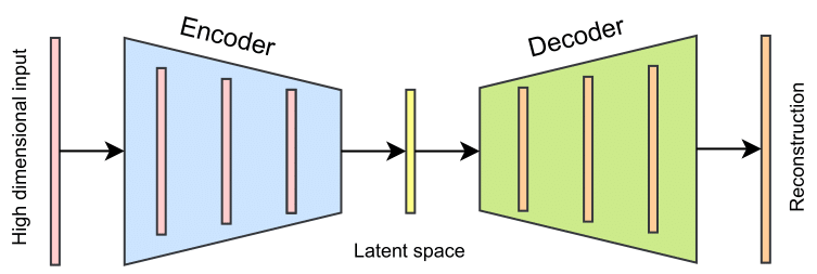
Figure 1: Illustration of an autoencoder network which encodes high dimensional inputs to latent space and decodes the latent space to reconstruct inputs.

3.4 Long short-term memory network

Recurrent neural networks (RNNs), designed to learn sequential data such as time series, address the stateless issue of classical MLP and CNN by allowing information to persist (Olah, 2015). Of particular interest, long short-term memory (LSTM) network, an advanced RNN architecture introduced by Hochreiter  Schmidhuber (1997), is able to handle vanishing and exploding gradients problem of RNN, and as a result, it accounts for long-term dependencies. An LSTM network is composed of multiple LSTM blocks consisting of LSTM layers. The LSTM layers are formed with interacting some LSTM units which are the smallest parts in the LSTM architecture.

3.4.1 LSTM unit

An LSTM unit shown in Figure 2 consists of a forget gate, an update gate, a cell state, and an output gate.

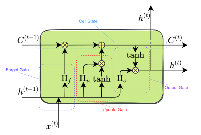
Figure 2: The architechture of an LSTM unit.

Forget gate

Input and hidden state data enter the forget gate $\mathbf{\Pi}_{f}$ of the LSTM cell. Forget gate is responsible for storing some information and discarding the rest by using a sigmoid function that is given as

$$\mathbf{\Pi}_{f}=\sigma(\mathbf{W}_{f}[\mathbf{h}^{(t-1)},\mathbf{x}^{(t)}]+\mathbf{b}_{f}).$$ (33)

Update gate

The second step is how much information is going to be kept in the cell state. Although $\mathbf{\Pi}_{u}$ in the update gate has the same mechanism as $\mathbf{\Pi}_{f}$ in the forget gate, their weights are different. The $\tanh$ normalizes data between -1 and 1 before sending it to $\mathbf{\Pi}_{u}$ for filtering and feature extraction as

$$\mathbf{\Pi}_{u}=\sigma(\mathbf{W}_{u}[\mathbf{h}^{(t-1)},\mathbf{x}^{(t)}]+\mathbf{b}_{u}),$$ (34)

$$\tilde{\mathbf{C}}^{(t)}=\text{tanh}(\mathbf{W}_{c}[\mathbf{h}^{(t-1)},\mathbf{x}^{(t)}]+\mathbf{b}_{c}).$$ (35)

Cell state

Insignificant information of the previous cell state entering into the LSTM unit is forgotten through the forget gate. Then, the important information of the cell state is updated through the update gate. As a result, forget and update gates extract features of the cell state that must be remembered. Cell state equation is as follows:

$$\mathbf{C}^{(t)}=\mathbf{\Pi}_{f}\odot\mathbf{C}^{(t-1)}+\mathbf{\Pi}_{u}\odot\tilde{\mathbf{C}}^{(t)},$$ (36)

where $\mathbf{C}^{(t)}$ shows current state of the cell. The gates regulate the LSTM unit to be able to remove or add information to the cell state, carefully regulated by structures called gates.

Output gate

Finally, the cell state for the next time step scaled with a $\tanh$ and filtered with $\mathbf{\Pi}_{o}$ makes the output. The output provides information that can be utilized for feeding the LSTM unit for the next time step and for the same time step in the next LSTM layer. The equations of the output gate and the next hidden state forecasting are given by:

$$\mathbf{\Pi}_{o}=\sigma(\mathbf{W}_{o}[\mathbf{h}^{(t-1)},\mathbf{x}^{(t)}]+\mathbf{b}_{o}),$$ (37)

$$\mathbf{h}^{(t)}=\mathbf{\Pi}_{o}\odot\text{tanh}(\mathbf{C}^{(t)}).$$ (38)

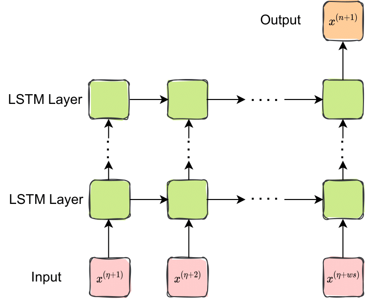
Figure 3: Input data $x$ is in red squares, output is in the orange square, and green squares represent hidden layers. The squares from left to right are in the same layer but in different times. The squares from below to up are at the same time but in different LSTM layers.

3.4.2 LSTM layers

The set of Eqs. 33–38 for the LSTM unit has the ability of predicting future state $x^{(n+1)}$ given $x^{(\eta+1)}$, $x^{(\eta+2)}$, $\dots$, $x^{(\eta+ws)}$, where $\eta=n-ws$. The $ws$ is referred to as the window size determining how many of previous time steps of the temporal information are required to accurately predict the future state of the system. As it can be seen in Figure 3, an LSTM network is built with many LSTM units in horizontal lines to create LSTM layers for complexity of the model and in vertical lines to keep information corresponding to a specific time step. Input data whose length is as same as the length of window size is fed to the first layer to predict the hidden state through a many-to-many layer. The following layer receives the hidden state and performs a similar operation. Finally, last layer, which is a many-to-one layer, forecasts the future state.

3.4.3 LSTM blocks

Instead of building an LSTM network by adding layers consecutively in series, we make the network with LSTM blocks. Figure 4 shows a network with one block, but we can connect multiple blocks to create a more complex LSTM network.

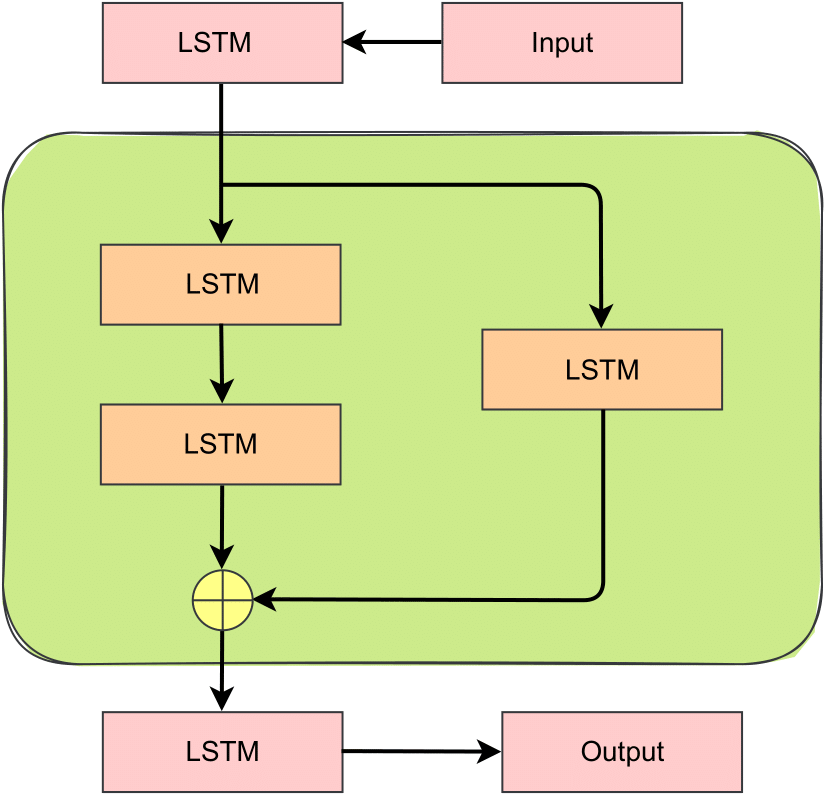
Figure 4: Building an LSTM network with LSTM blocks rather than stacking layers consecutively.

3.5 Nonlinear proper orthogonal decomposition

High dimensional data cannot be accurately reconstructed with limited number of POD modes. Consequently, we choose higher number of POD modes or RIC and remove further uncorrelated data with utilizing autoencoder technology to consider under-resolved flow and to reduce projection error - the error between true projection and NIROM. In this regard, POD temporal coefficients are fed into multi-layer perceptron AE network to learn much lower dimensional latent space than the number of POD modes. Then, the latent space data is used as input data for LSTM network for time evolution of the low-rank space. In order to reconstruct high dimensional data in the desired time, first we decode the latent space information after LSTM forecasting, and then, we multiply decoded data or POD temporal coefficients to basis functions.

4 Numerical results

We employ the NLPOD framework to forecast temperature in the 2D Rayleigh–Bénard convection flow. In order to simulate the flow field and acquire the FOM data, we first perform numerical simulations for the $\text{Ra}=2\times 10^{6}$, $\text{Ra}=9\times 10^{6}$, and $\text{Ra}=1\times 10^{7}$ cases on a computational domain covered by $512\times 256$ nodes. We collect the temperature field as the FOM data only after the initial transient region. After taking SVD from $131072$ nodes and keeping $99\%$ of the content, we get $N_{R}=8,\;28,\;45$ number of POD modes for the $\text{Ra}=2\times 10^{6},\;\text{Ra}=9\times 10^{6},\;\text{Ra}=1\times 10^{7}$, respectively. We encode the POD modes to reduce the dimension to only $N_{r}=4$ time series before feeding it to the LSTM network for learning time dependencies.

Training sets for all cases in this paper are from $t=0$ to $t=175$ s, which has colored background in our resulting figures. Out of sample data is illustrated with white background. We apply the SVD only on the training sets to get the basis functions and employ those basis functions to reconstruct extrapolated temperature field. We show results only starting from $t=150$ s to remove redundancy. For the rest of this study, we depict the FOM, true projection (TP), and mean values as a solid black line, dash-dot green line, and dashed red line, respectively. The forecasted solution with the AE network is shown by the solid blue line.

In order to thoroughly investigate LSTM performance combined with NLPOD, we train 64 models with different hyperparameters (see Table 1), such as learning rate, activation function, optimizer, initialization, number of LSTM units, and number of LSTM blocks. Our analysis also provides the mean $\mu$ and the two standard deviation (SD) bounds $\mu\mp 2\times\text{SD}$.

Table 1: Hyperparameters used in long short-term memory (LSTM) networks. We note that our analysis involves 64 different LSTM models.

Parameters	Range of consideration
Learning rate	[0.001, 0.0001]
Activation function	[tanh, relu]
Optimizer	[adam, rmsprop]
Initialization	[uniform, Glorot]
Number of LSTM units	[10, 20]
Number of LSTM block	[2, 3]

4.1 $Ra=2\times 10^{6}$Case

For almost periodic dynamics case with $\text{Ra}=2\times 10^{6}$, Figure 5 shows that $4$ POD modes are able to achieve $93.52\%$ of the RIC and $8$ modes are needed to capture $99\%$ of the content.

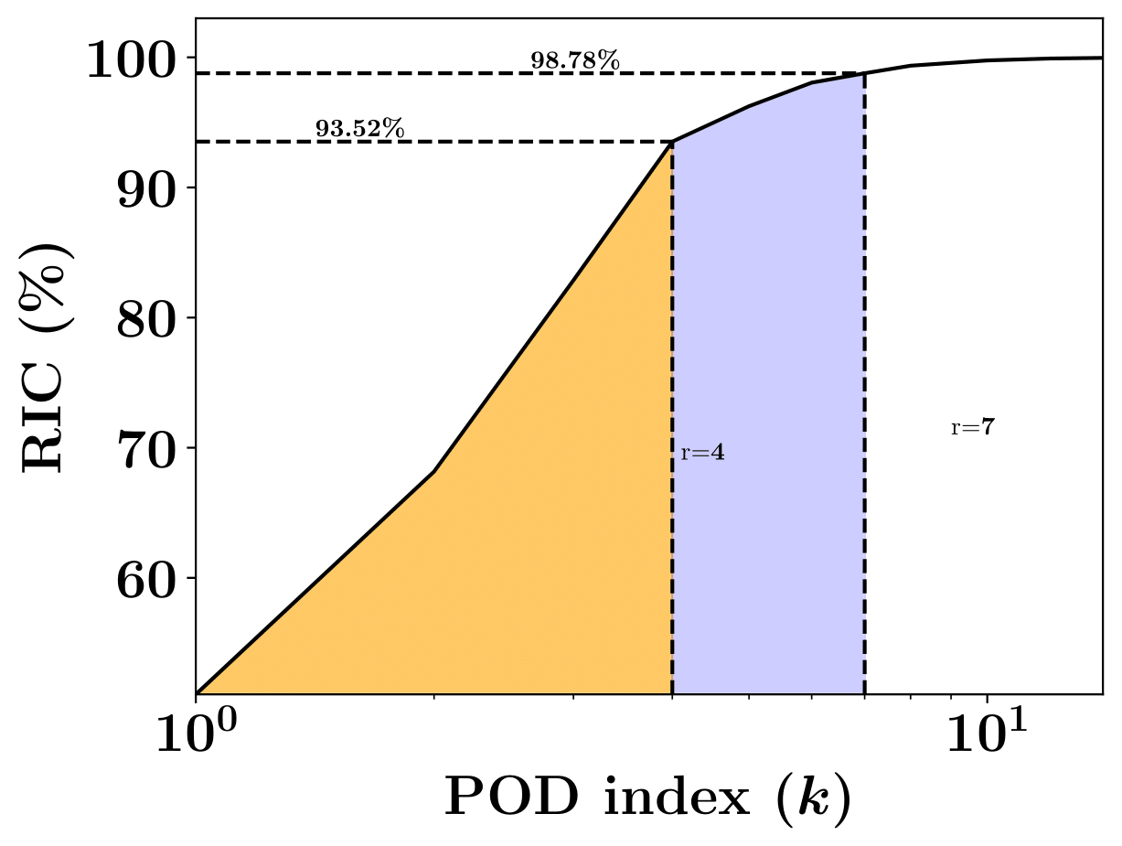
Figure 5: The relative information content based on number of retained modes for $\text{Ra}=2\times 10^{6}$. While the leading $4$ POD modes capture $93.52\%$, the first $8$ POD modes are able to capture more that $99\%$ of the relative information content of the high dimensional data. As a result, the suggested AE is constructed to learn a latent space from $8$ POD coefficients.

Figure 6 shows the time evolution of the first $4$ POD modes for $\text{Ra}=2\times 10^{6}$. It can be seen that the AE reconstruction is very accurate for an almost time periodic dynamical system. Therefore, $N_{r}=4$ is sufficient for this case to reconstruct the POD modes and finally the temperature from the latent space.

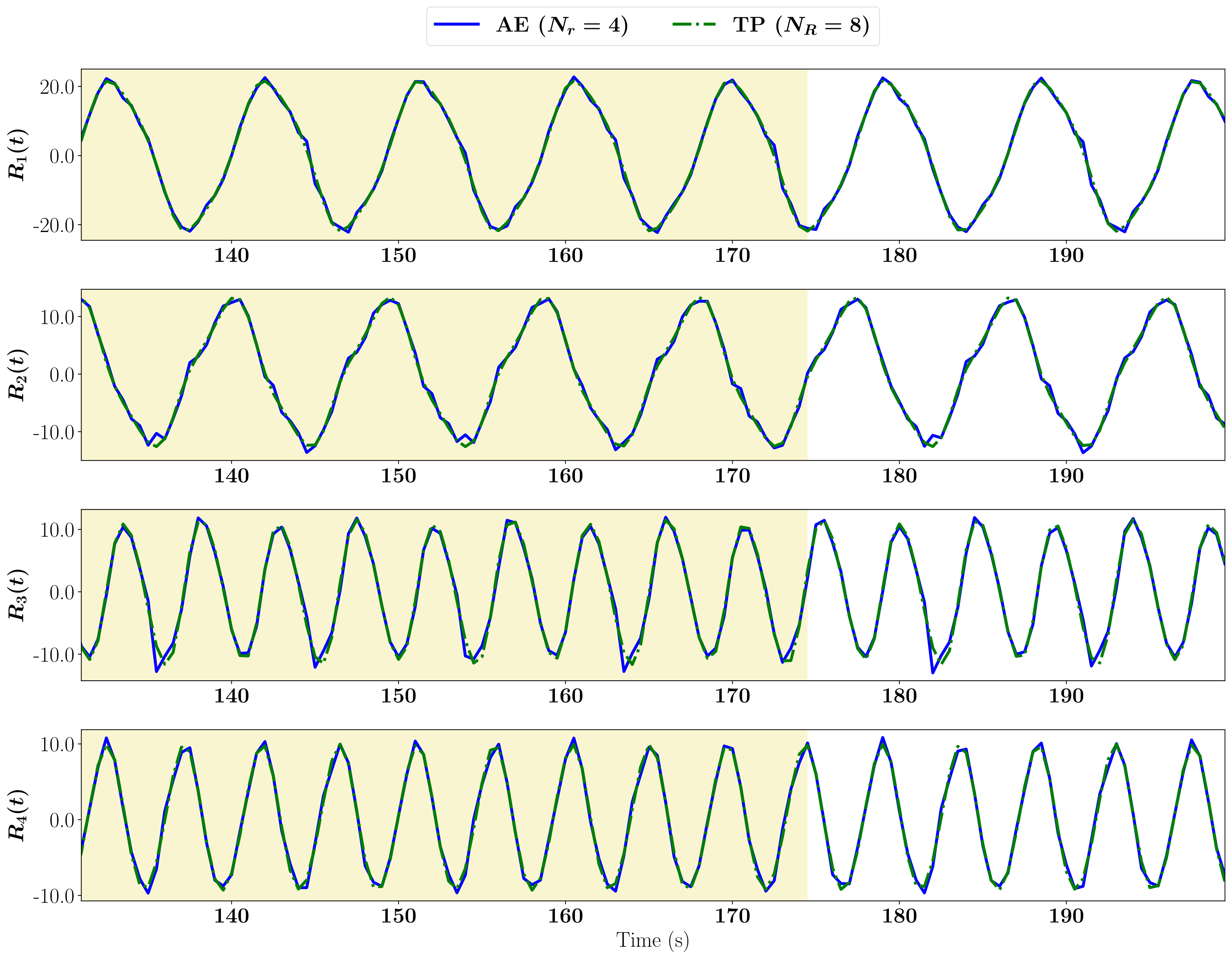
Figure 6: Evolution of the first four POD modal coefficients for $\text{Ra}=2\times 10^{6}$. The training set for the AE network is from $t=0$ to $t=175$ s.

Figure 7 presents the time evolution of four time series in the latent space of the AE network using the data for $\text{Ra}=2\times 10^{6}$. The purpose of this plot is to reveal how LSTM performs on predicting of the almost periodic time series. As it is illustrated in Figure 7, the SD bars are quite close to the mean value, meaning we do not need to spend resources for tuning the network to get accurate prediction as long as hyperparameters are in a reasonable range.

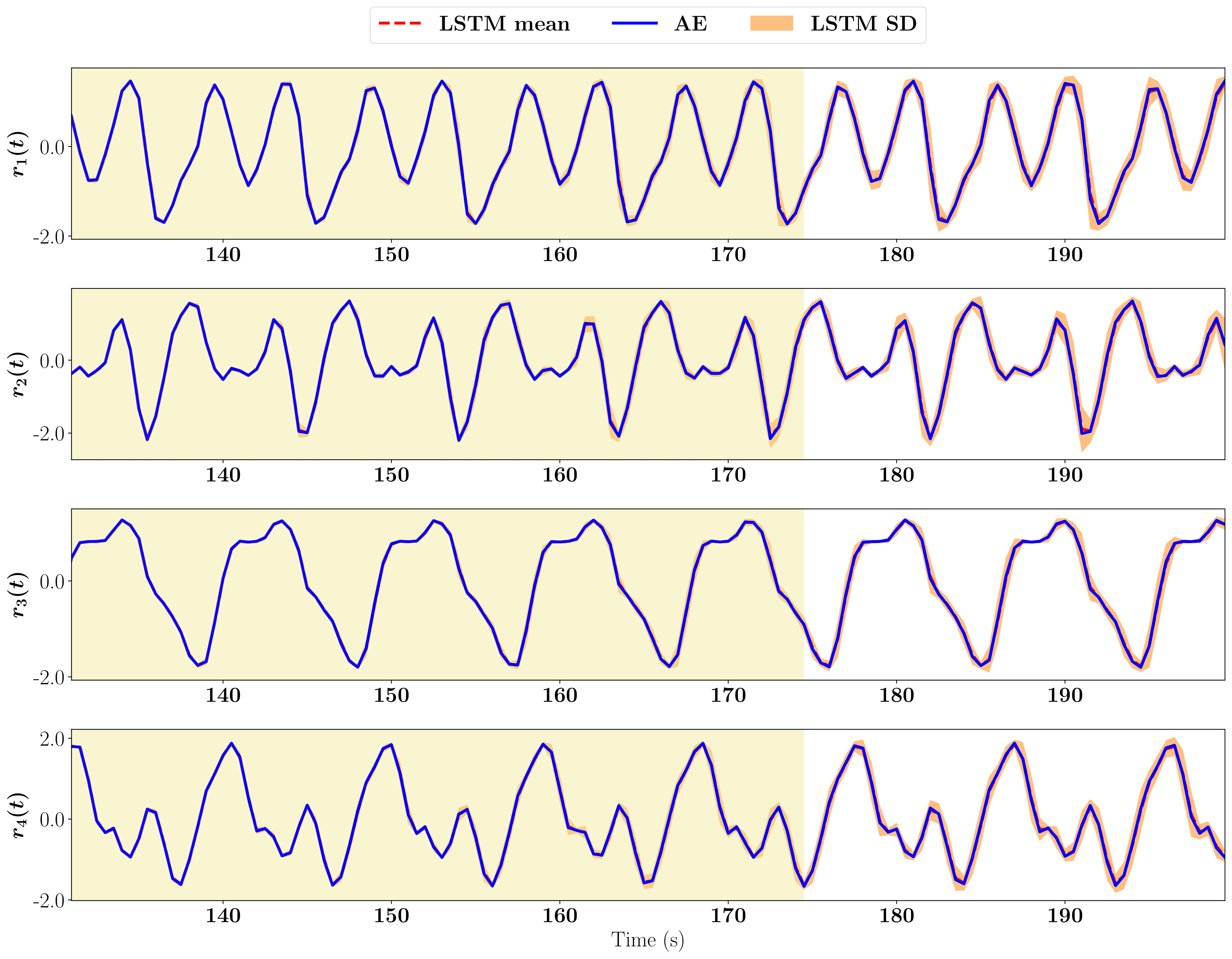
Figure 7: Evolution of autoencoder modes in latent space with the LSTM for $\text{Ra}=2\times 10^{6}$. The training set for the LSTM network is from $t=0$ to $t=175$ s.

Figure 8 plots reconstructed temperature on the four points. As we expect based on the performance of AE and LSTM, farecasted temperature with NLPOD is able to follow the TP curve which is quite close to the FOM solution. As a result, NLPOD is quite accurate for flows with almost periodic dynamics. This can also be seen from Figure 9 when we compare temperature fields for $\text{Ra}=2\times 10^{6}$ at two different times.

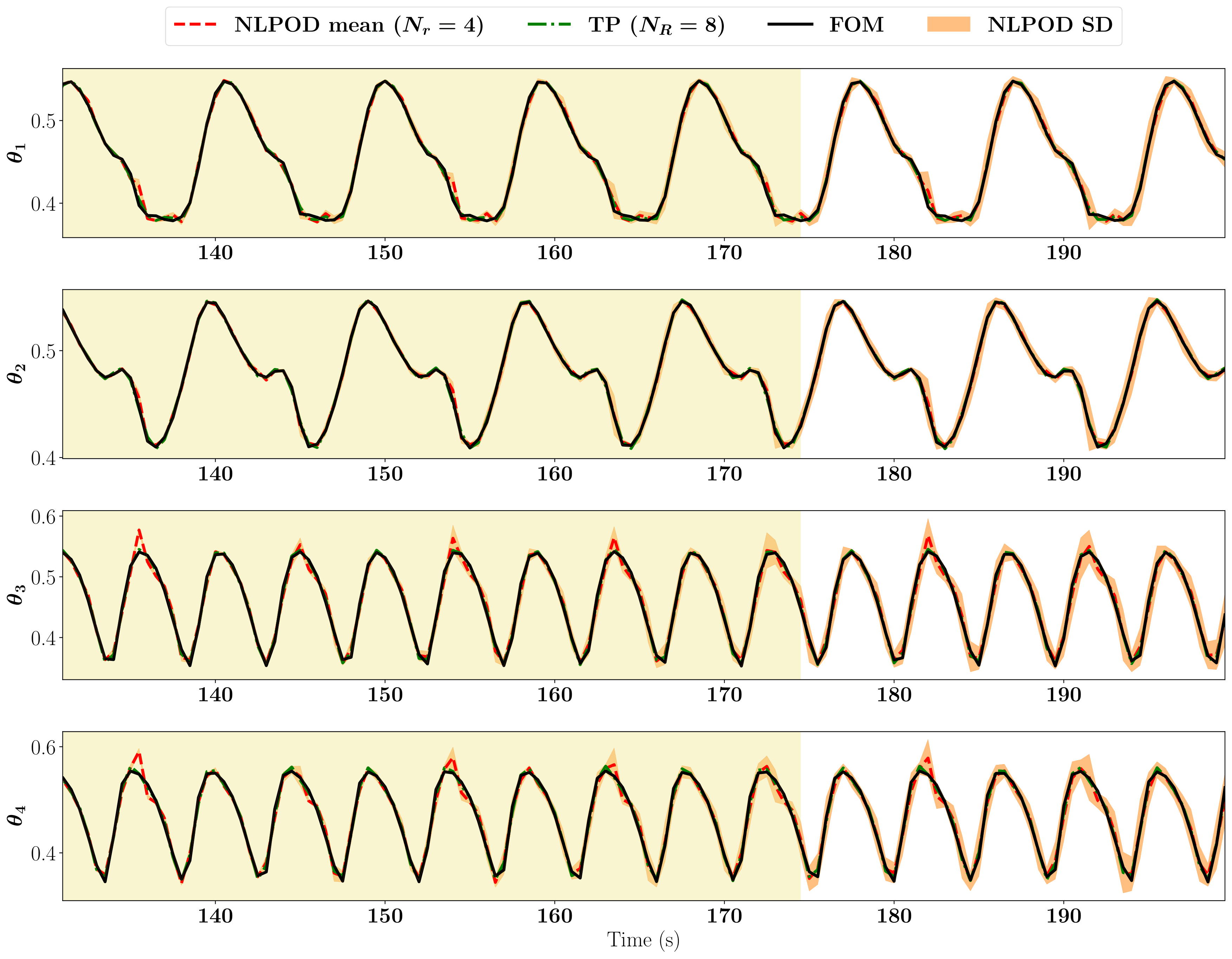
Figure 8: Temperature evolution in physical space for $\text{Ra}=2\times 10^{6}$ at four locations.

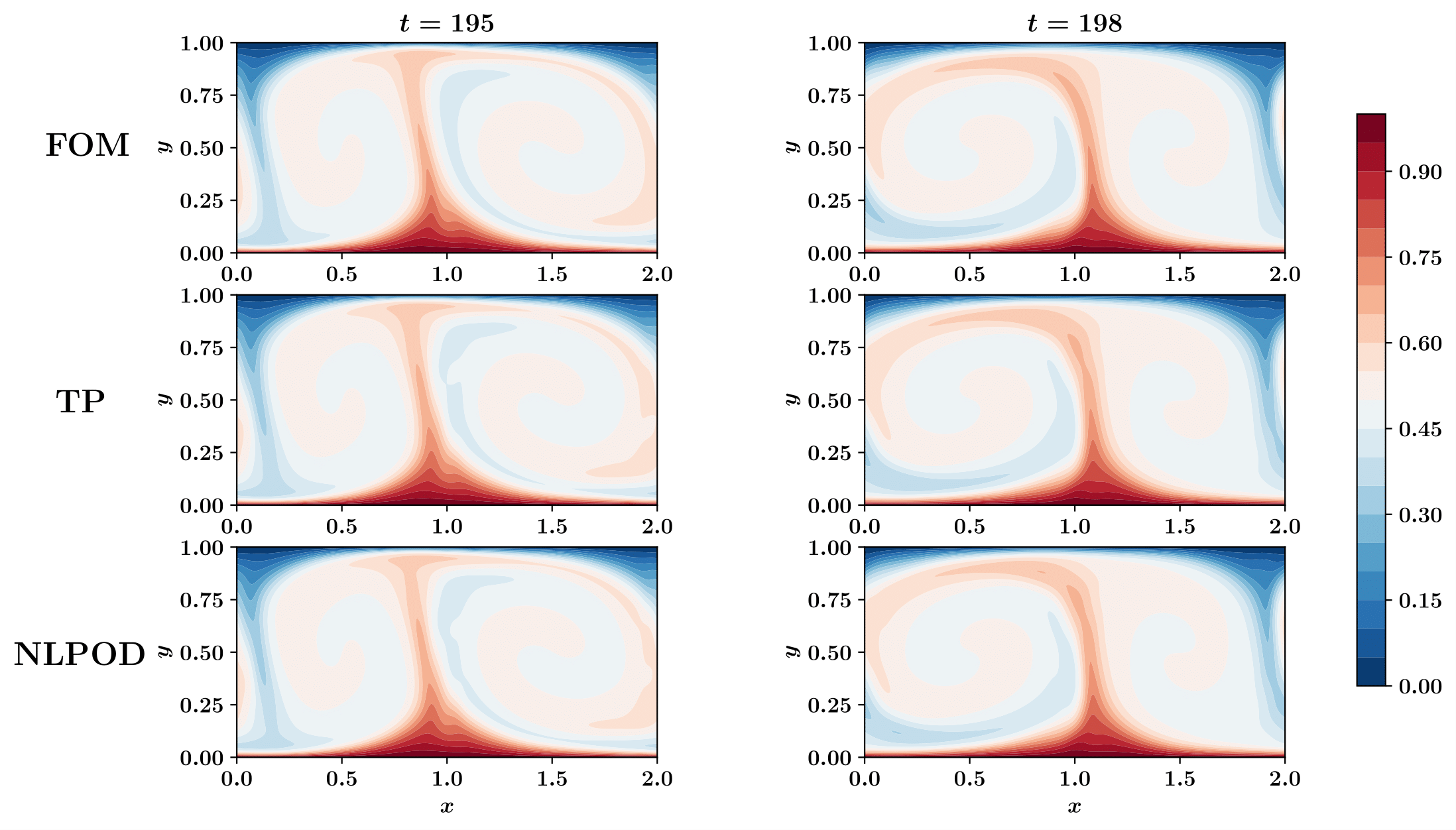
Figure 9: A comparison of temperature fields for $\text{Ra}=2\times 10^{6}$ at two different times.

4.2 $Ra=9\times 10^{6}$Case

For quasi-periodic dynamics with $\text{Ra}=9\times 10^{6}$, Figure 10 shows that $4$ POD modes have the ability to acheive $83.45\%$ of the RIC and $28$ modes are needed to capture more than $99\%$ of the content.

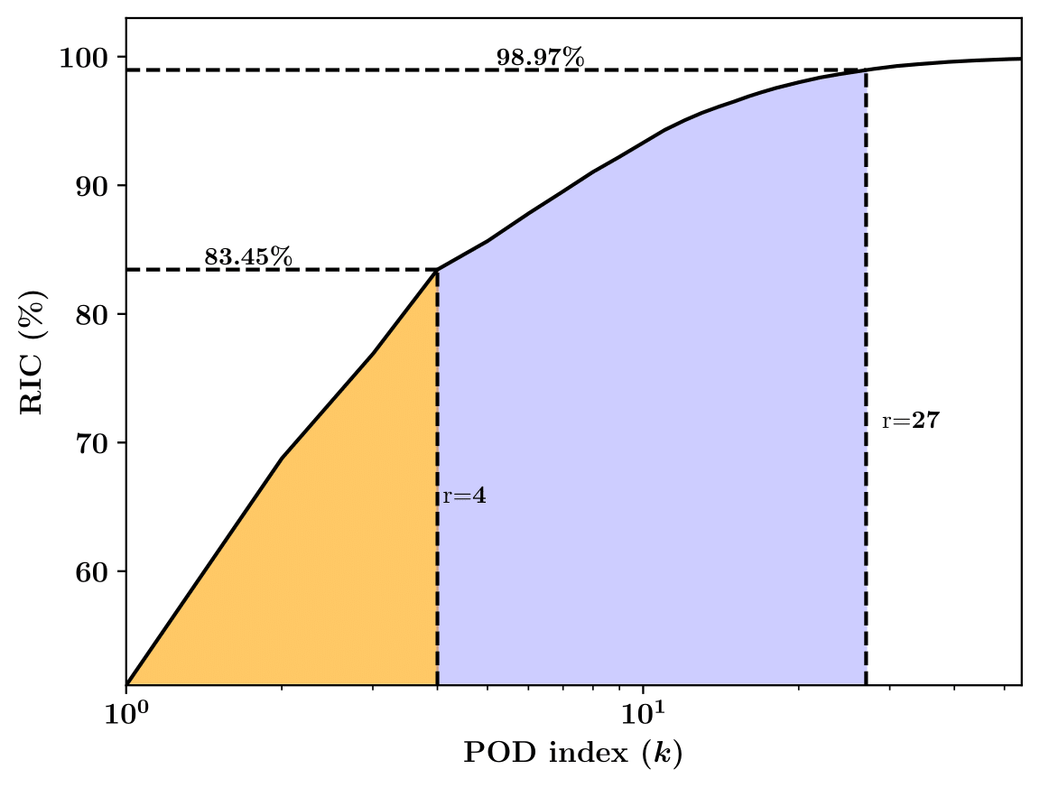
Figure 10: The relative information content based on number of retained modes for $\text{Ra}=9\times 10^{6}$. While the leading $4$ POD modes capture $83.45\%$, the first $28$ POD modes are able to capture more that $99\%$ of the relative information content of the high dimensional data. As a result, the suggested AE is constructed to learn a latent space from $28$ POD coefficients.

Figure 11 illustrates the time evolution of the first $4$ POD modes for $\text{Ra}=9\times 10^{6}$. It can still be seen that the AE reconstruction is pretty close for a quasi-periodic dynamical system, and as a result, the AE is not a bottleneck for this case with $\text{Ra}=9\times 10^{6}$.

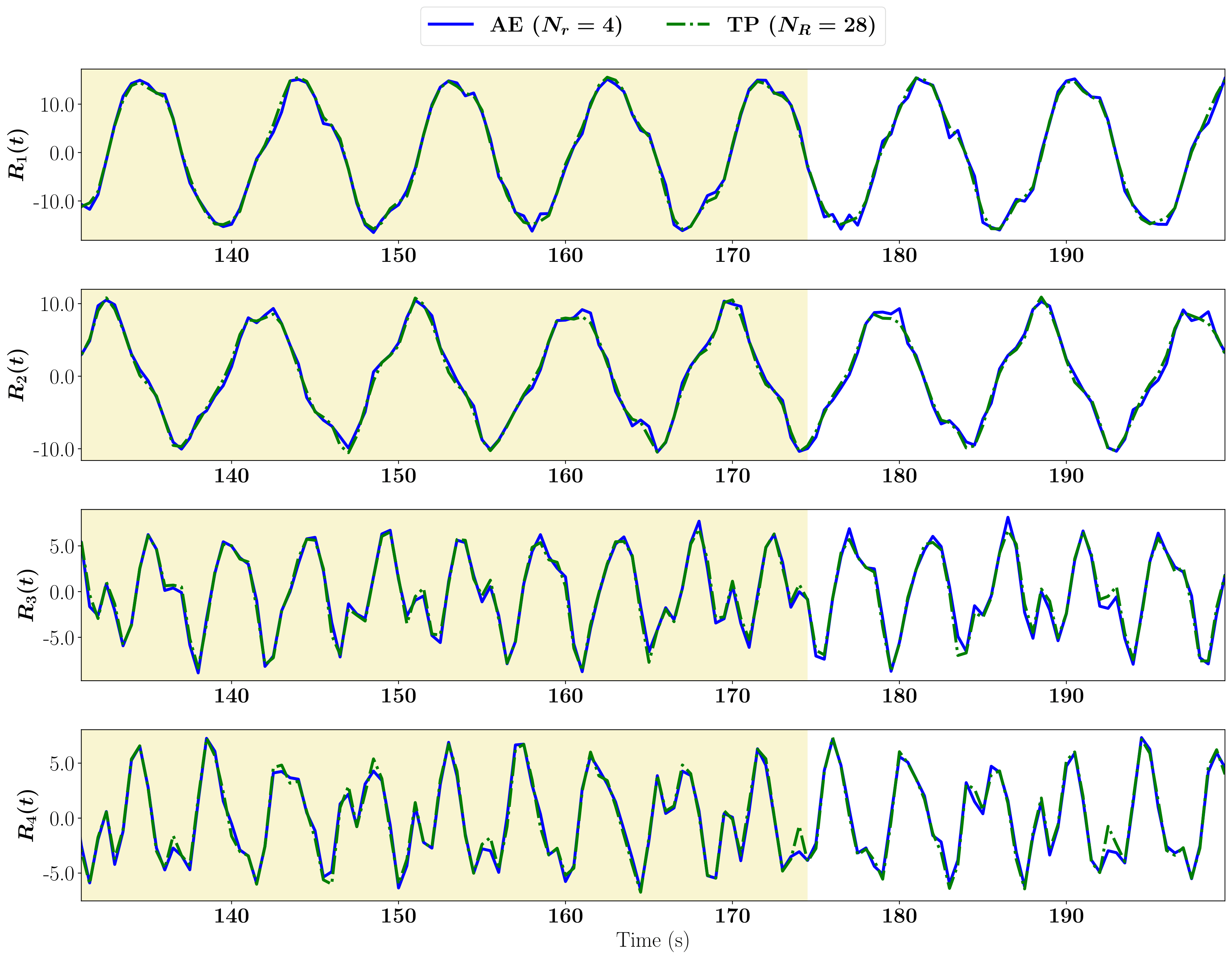
Figure 11: Variation of first four POD temporal coefficients for $\text{Ra}=9\times 10^{6}$. The training set for the AE network is from $t=0$ to $t=175$ s.

Figure 12 illustrates the time evolution in the latent space for four neurons of the AE network utilizing the data for $\text{Ra}=9\times 10^{6}$. Our aim of drawing this figure is to demonstrate the LSTM performance is accurate for quasi-periodic dynamics in the latent space of AE with some hyperparameter tuning. As it is shown in Figure 12 the SD bars are close to the mean value in the interpolatory region, but they have a little more width in the extrapolatory region.

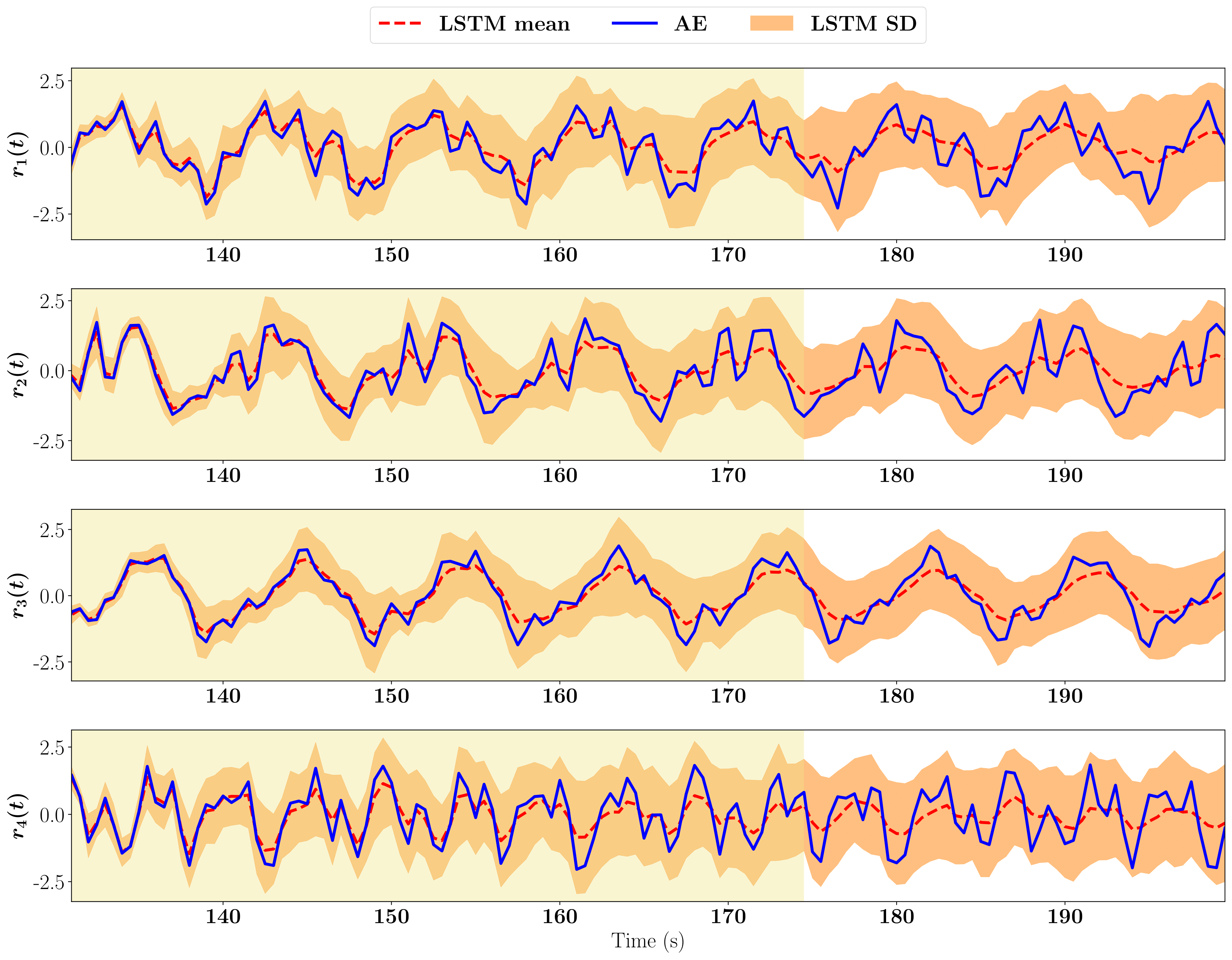
Figure 12: Evolution of autoencoder modes in latent space with the LSTM for $\text{Ra}=9\times 10^{6}$. The training set for the LSTM network is from $t=0$ to $t=175$ s.

Figure 13 compares the reconstructed temperature field of FOM, TP, and NLPOD at four locations. According to Figure 13, TP is close to FOM data because we retain $99\%$ of content by keeping $28$ POD modes. This is also verified in Figure 14 for the reconstruction of the temperature fields at two different times.

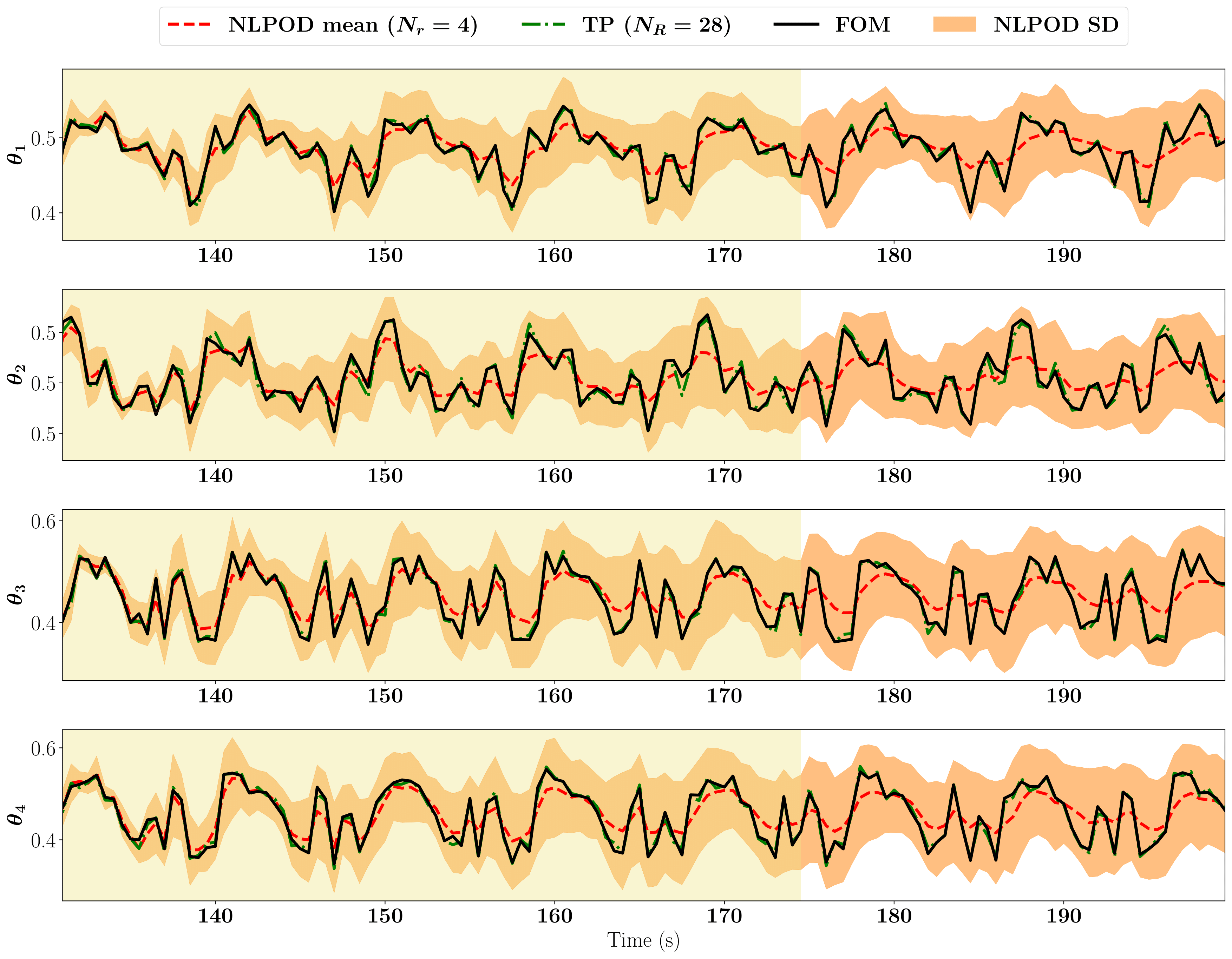
Figure 13: Temperature evolution in physical space for $\text{Ra}=9\times 10^{6}$ at four locations.

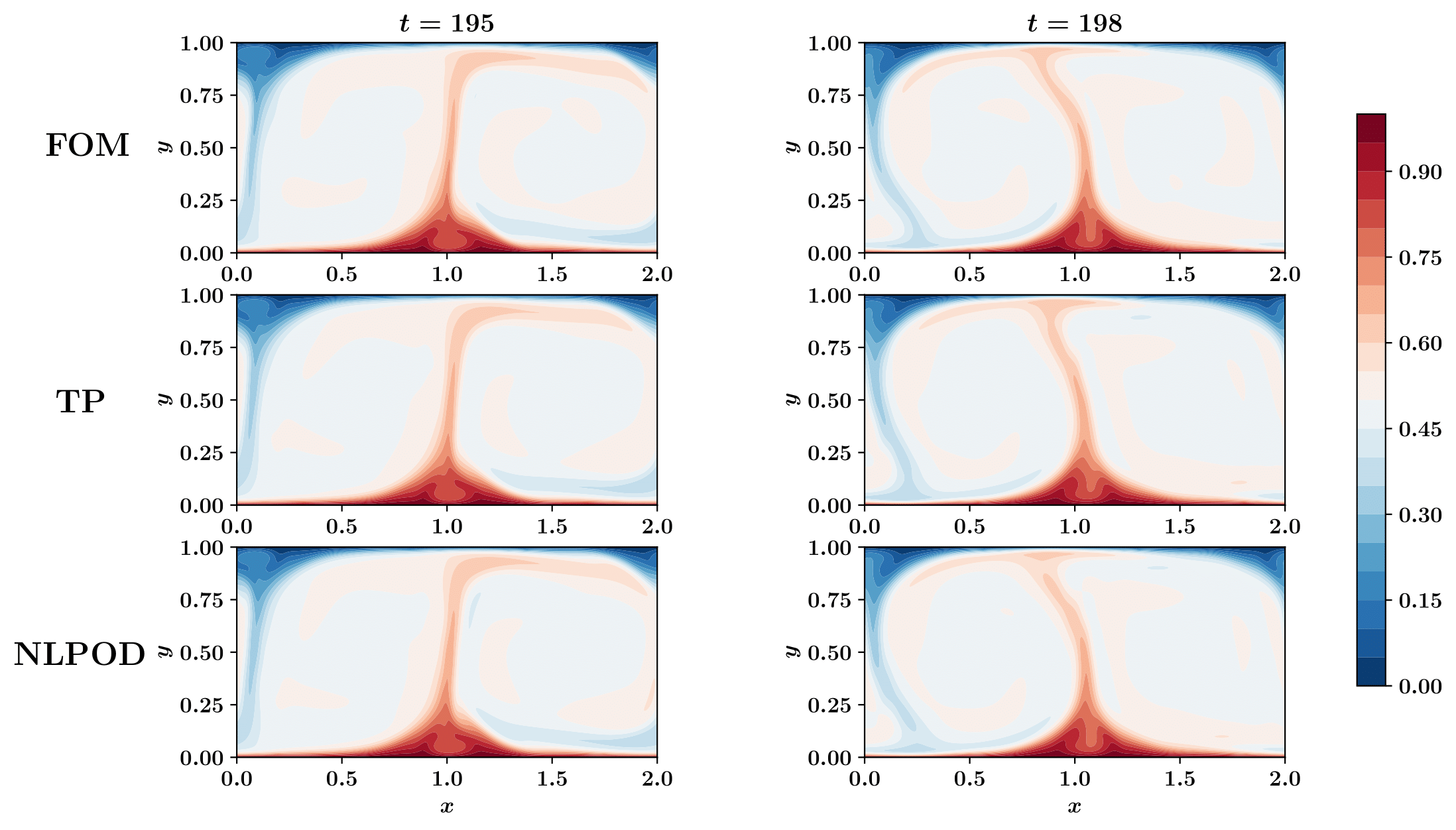
Figure 14: A comparison of temperature fields for $\text{Ra}=9\times 10^{6}$ at two different times.

4.3 $Ra=1\times 10^{7}$Case

For almost chaotic dynamics or irregular dynamics with $\text{Ra}=1\times 10^{7}$, Figure 15 illustrates that $4$ POD modes have the ability to attain $77.62\%$ of the RIC and $45$ modes are required to capture more than $99\%$ of the energy.

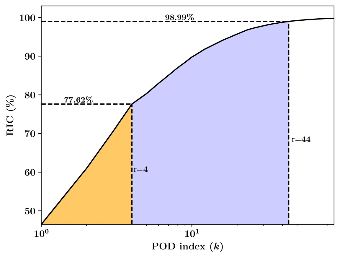
Figure 15: The relative information content based on number of retained modes for $\text{Ra}=1\times 10^{7}$. While the leading $4$ POD modes capture $77.62\%$, the first $45$ POD modes are able to capture more that $99\%$ of the relative information content of the high dimensional data. As a result, the suggested AE is constructed to learn a latent space from $45$ POD coefficients.

Figure 16 presents the time variation of the first $4$ POD modes for $\text{Ra}=1\times 10^{7}$. Although the AE is able to reconstruct the $45$ POD modes with $4$ neurons in the latent space, there is a little discrepancy between AE and TP curves. Besides, the LSTM network has to learn the curve that AE makes. Consequently, the more chaos curve AE makes the more arduous is for LSTM to follow the curve. Having said that, to build NLPOD models for higher Ra numbers we need to focus on AE network too as the AE is going to be a bottleneck. Otherwise, we are not going to reduce data to a few modes.

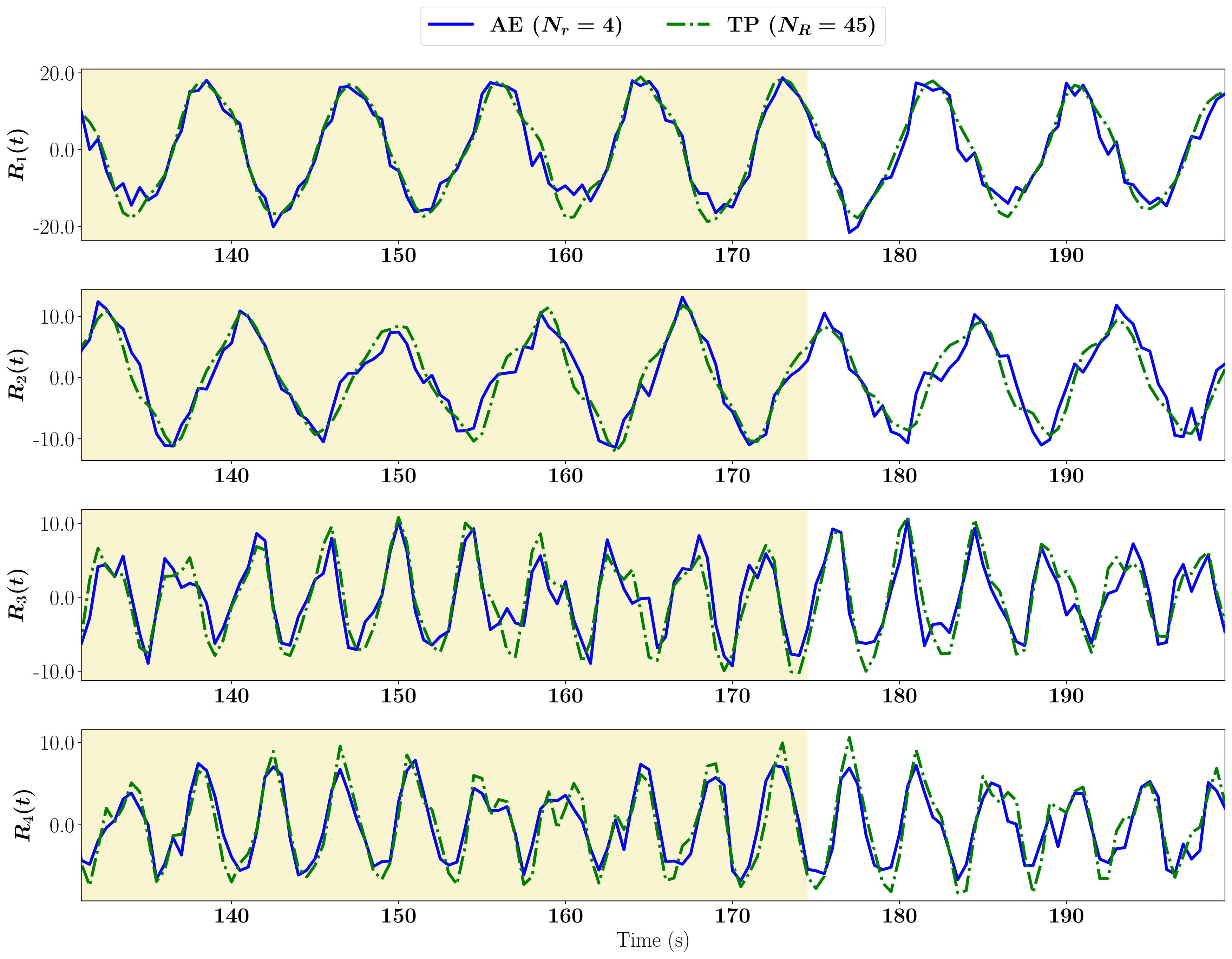
Figure 16: Variation of first four POD temporal coefficients for $\text{Ra}=1\times 10^{7}$. The training set for the AE network is from $t=0$ to $t=175$ s.

Figure 17 shows the time evolution of the first four AE modes for $\text{Ra}=1\times 10^{7}$. The aim of this plot is to show how LSTM performs on predicting of the almost chaotic dynamics or irregular dynamic time series. Although the LSTM can capture low frequency parts of the curve, its prediction is not able to exactly match the high frequency parts. It also shows that in the extrapolatory region, there is a shift between the LSTM prediction and the AE prediction. The SD bars cover the AE curve. In other words, our 64 LSTM models can provide us with a bound that we are certain it covers the true or AE curve.

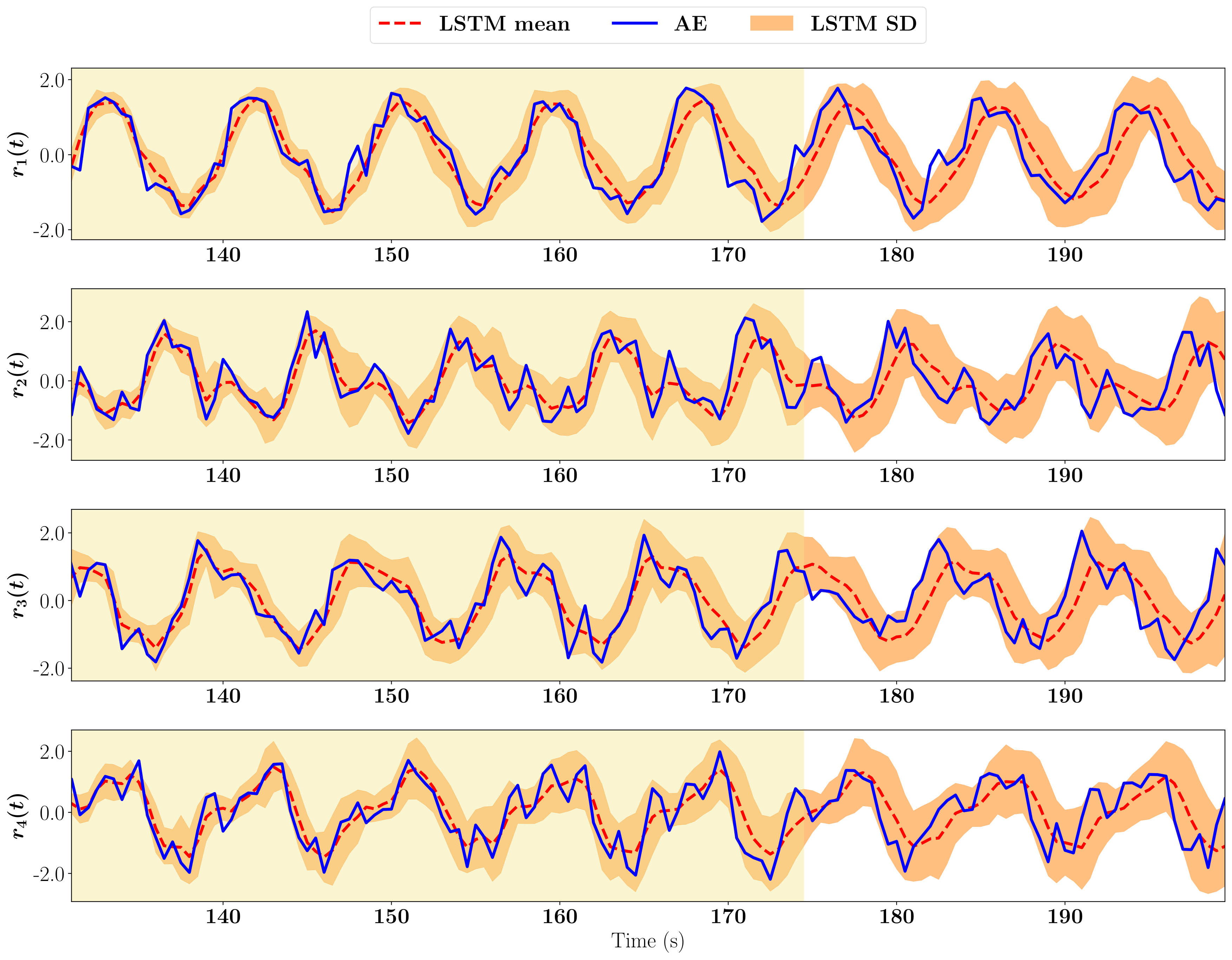
Figure 17: Evolution of autoencoder modes in latent space with the LSTM for $\text{Ra}=1\times 10^{7}$. The training set for the LSTM network is from $t=0$ to $t=175$ s.

In Figure 18, TP is still very close to FOM curve since we remove uncorrelated data in two steps employing POD and AE instead of cutting all the modes from the mesh size to $4$ with only POD. Figure 18 where we observe the capability of the NLPOD to reconstruct trends for temperature field in the physical space from few modes.

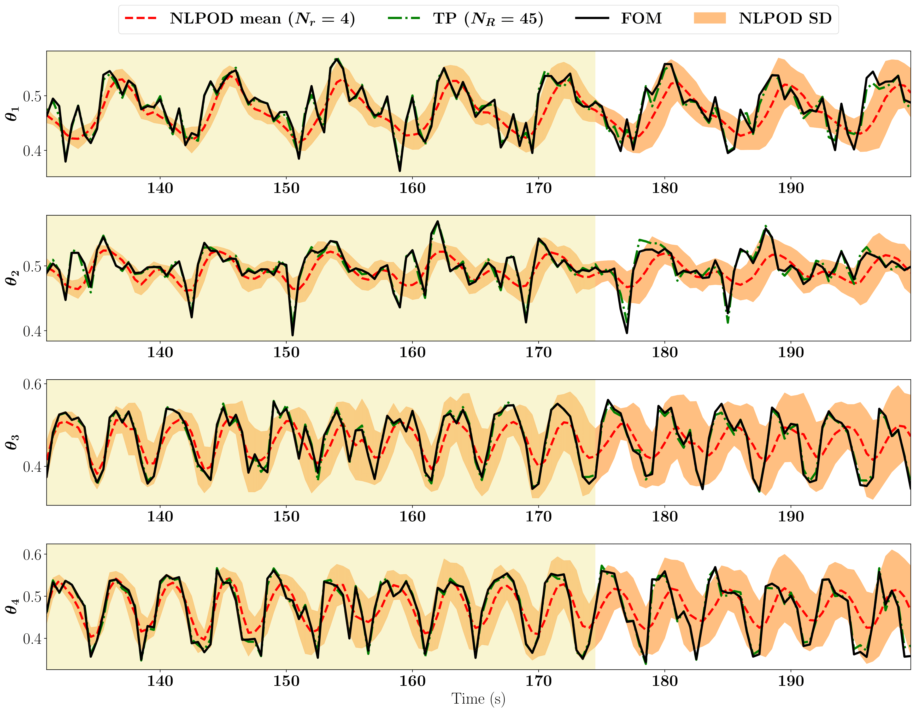
Figure 18: Temperature evolution in physical space for $\text{Ra}=1\times 10^{7}$ at four locations.

Figure 19 shows temperature contours at two different times. The coherent structures of the temperature fields are reconstructed by the NLPOD compared with both TP and FOM.

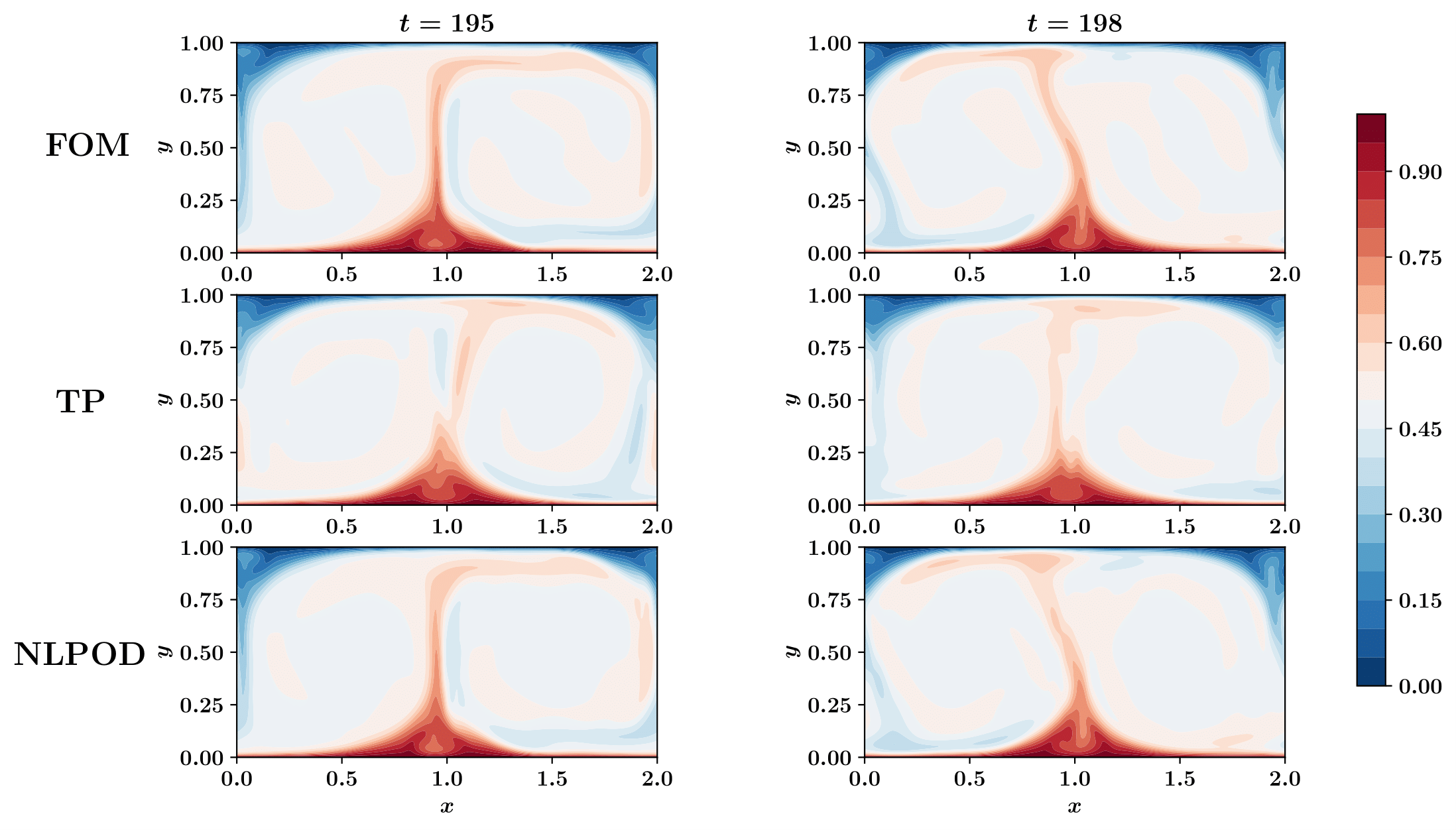
Figure 19: A comparison of temperature fields for $\text{Ra}=1\times 10^{7}$ at two different times.

5 Concluding remarks

In this study, we investigate a nonintrusive reduced order model (ROM) for convection-dominated fluid flows that can be used for other nonlinear continuum phenomena. Our ROM, nonlinear proper orthogonal decomposition (NLPOD), is based on a proper orthogonal decomposition to recognize dominant but linear patterns from the data and to utilize an autoencoder technology with perceptron layers for further reduction and nonlinear pattern identification. Then, we use a long short term memory architecture to learn the dynamics of low fidelity data in latent space. This data-driven modeling approach relies on only stored data and can be applied without having access to the governing equations.

While the approach does not completely lift the Kolmogorov barrier, based on our analysis we found that the NLPOD significantly reduces the number of degrees of freedom needed to represent the underlying dynamics. Indeed, the degree of irregularity increases as the Rayleigh number rises, producing a more chaotic or turbulent spatiotemporal dynamics. We also highlight that the full order model dimension can be on the order of billions (and even higher) for three-dimensional turbulent industrial or geophysical flows. In those cases, the NLPOD approach might still reduce the ROM dimension to a handful of latent variables if there are spatiotemporal structures. However, while the Kolmogorov n-width increases, the models’ uncertainty grows as shown in our results. By defining feasible maps between the observation space and the latent variables, a viable method for minimizing the uncertainty of such ROM solutions might be to use nonlinear filtering or dynamic data assimilation techniques, a topic we plan to address in a subsequent paper.

Data availability

The data that support the findings of this study are available within the article. The datasets used and/or analysed during the current study are available from the corresponding author on reasonable request. The implementation and open-source Python codes are available at https://github.com/Saeed-Akbari/POD-AE-LSTM.

Disclosure statement

We declare we have no competing interests.

Funding

This material is based upon work supported by the U.S. Department of Energy, Office of Science, Office of Advanced Scientific Computing Research under Award Number DE-SC0019290. O.S. gratefully acknowledges their support.

Disclaimer: This report was prepared as an account of work sponsored by an agency of the United States Government. Neither the United States Government nor any agency thereof, nor any of their employees, makes any warranty, express or implied, or assumes any legal liability or responsibility for the accuracy, completeness, or usefulness of any information, apparatus, product, or process disclosed, or represents that its use would not infringe privately owned rights. Reference herein to any specific commercial product, process, or service by trade name, trademark, manufacturer, or otherwise does not necessarily constitute or imply its endorsement, recommendation, or favoring by the United States Government or any agency thereof. The views and opinions of authors expressed herein do not necessarily state or reflect those of the United States Government or any agency thereof.

References

- Abadía-Heredia \BOthers. (\APACyear2022) \APACinsertmetastarabadia2022predictive{APACrefauthors}Abadía-Heredia, R., López-Martín, M., Carro, B., Arribas, J\BPBII., Pérez, J\BPBIM.\BCBL \BBA Le Clainche, S. \APACrefYearMonthDay2022. \BBOQ\APACrefatitleA predictive hybrid reduced order model based on proper orthogonal decomposition combined with deep learning architectures A predictive hybrid reduced order model based on proper orthogonal decomposition combined with deep learning architectures.\BBCQ \APACjournalVolNumPagesExpert Systems with Applications187115910. \PrintBackRefs\CurrentBib
- M. Ahmed \BBA San (\APACyear2018) \APACinsertmetastarahmed2018stabilized{APACrefauthors}Ahmed, M.\BCBT \BBA San, O. \APACrefYearMonthDay2018. \BBOQ\APACrefatitleStabilized principal interval decomposition method for model reduction of nonlinear convective systems with moving shocks Stabilized principal interval decomposition method for model reduction of nonlinear convective systems with moving shocks.\BBCQ \APACjournalVolNumPagesComputational and Applied Mathematics3756870–6902. \PrintBackRefs\CurrentBib
- S\BPBIE. Ahmed, Pawar\BCBL \BOthers. (\APACyear2021) \APACinsertmetastarahmed2021closures{APACrefauthors}Ahmed, S\BPBIE., Pawar, S., San, O., Rasheed, A., Iliescu, T.\BCBL \BBA Noack, B\BPBIR. \APACrefYearMonthDay2021. \BBOQ\APACrefatitleOn closures for reduced order models—A spectrum of first-principle to machine-learned avenues On closures for reduced order models—a spectrum of first-principle to machine-learned avenues.\BBCQ \APACjournalVolNumPagesPhysics of Fluids339091301. \PrintBackRefs\CurrentBib
- S\BPBIE. Ahmed \BBA San (\APACyear2020) \APACinsertmetastarahmed2020breaking{APACrefauthors}Ahmed, S\BPBIE.\BCBT \BBA San, O. \APACrefYearMonthDay2020. \BBOQ\APACrefatitleBreaking the Kolmogorov barrier in model reduction of fluid flows Breaking the Kolmogorov barrier in model reduction of fluid flows.\BBCQ \APACjournalVolNumPagesFluids5126. \PrintBackRefs\CurrentBib
- S\BPBIE. Ahmed \BOthers. (\APACyear2020) \APACinsertmetastarahmed2020long{APACrefauthors}Ahmed, S\BPBIE., San, O., Rasheed, A.\BCBL \BBA Iliescu, T. \APACrefYearMonthDay2020. \BBOQ\APACrefatitleA long short-term memory embedding for hybrid uplifted reduced order models A long short-term memory embedding for hybrid uplifted reduced order models.\BBCQ \APACjournalVolNumPagesPhysica D: Nonlinear Phenomena409132471. \PrintBackRefs\CurrentBib
- S\BPBIE. Ahmed, San\BCBL \BOthers. (\APACyear2021) \APACinsertmetastarahmed2021nonlinear{APACrefauthors}Ahmed, S\BPBIE., San, O., Rasheed, A.\BCBL \BBA Iliescu, T. \APACrefYearMonthDay2021. \BBOQ\APACrefatitleNonlinear proper orthogonal decomposition for convection-dominated flows Nonlinear proper orthogonal decomposition for convection-dominated flows.\BBCQ \APACjournalVolNumPagesPhysics of Fluids3312121702. \PrintBackRefs\CurrentBib
- Amsallem \BBA Haasdonk (\APACyear2016) \APACinsertmetastaramsallem2016pebl{APACrefauthors}Amsallem, D.\BCBT \BBA Haasdonk, B. \APACrefYearMonthDay2016. \BBOQ\APACrefatitlePEBL-ROM: Projection-error based local reduced-order models Pebl-rom: Projection-error based local reduced-order models.\BBCQ \APACjournalVolNumPagesAdvanced Modeling and Simulation in Engineering Sciences311–25. \PrintBackRefs\CurrentBib
- Amsallem \BOthers. (\APACyear2012) \APACinsertmetastaramsallem2012nonlinear{APACrefauthors}Amsallem, D., Zahr, M\BPBIJ.\BCBL \BBA Farhat, C. \APACrefYearMonthDay2012. \BBOQ\APACrefatitleNonlinear model order reduction based on local reduced-order bases Nonlinear model order reduction based on local reduced-order bases.\BBCQ \APACjournalVolNumPagesInternational Journal for Numerical Methods in Engineering9210891–916. \PrintBackRefs\CurrentBib
- Amsallem \BOthers. (\APACyear2015) \APACinsertmetastaramsallem2015fast{APACrefauthors}Amsallem, D., Zahr, M\BPBIJ.\BCBL \BBA Washabaugh, K. \APACrefYearMonthDay2015. \BBOQ\APACrefatitleFast local reduced basis updates for the efficient reduction of nonlinear systems with hyper-reduction Fast local reduced basis updates for the efficient reduction of nonlinear systems with hyper-reduction.\BBCQ \APACjournalVolNumPagesAdvances in Computational Mathematics4151187–1230. \PrintBackRefs\CurrentBib
- Aubry \BOthers. (\APACyear1993) \APACinsertmetastaraubry1993preserving{APACrefauthors}Aubry, N., Lian, W\BHBIY.\BCBL \BBA Titi, E\BPBIS. \APACrefYearMonthDay1993. \BBOQ\APACrefatitlePreserving symmetries in the proper orthogonal decomposition Preserving symmetries in the proper orthogonal decomposition.\BBCQ \APACjournalVolNumPagesSIAM Journal on Scientific Computing142483–505. \PrintBackRefs\CurrentBib
- Bergmann \BOthers. (\APACyear2009) \APACinsertmetastarbergmann2009enablers{APACrefauthors}Bergmann, M., Bruneau, C\BHBIH.\BCBL \BBA Iollo, A. \APACrefYearMonthDay2009. \BBOQ\APACrefatitleEnablers for robust POD models Enablers for robust pod models.\BBCQ \APACjournalVolNumPagesJournal of Computational Physics2282516–538. \PrintBackRefs\CurrentBib
- Berkooz \BOthers. (\APACyear1993) \APACinsertmetastarberkooz1993proper{APACrefauthors}Berkooz, G., Holmes, P.\BCBL \BBA Lumley, J\BPBIL. \APACrefYearMonthDay1993. \BBOQ\APACrefatitleThe proper orthogonal decomposition in the analysis of turbulent flows The proper orthogonal decomposition in the analysis of turbulent flows.\BBCQ \APACjournalVolNumPagesAnnual review of fluid mechanics251539–575. \PrintBackRefs\CurrentBib
- Briley (\APACyear1971) \APACinsertmetastarbriley1971numerical{APACrefauthors}Briley, W\BPBIR. \APACrefYearMonthDay1971. \BBOQ\APACrefatitleA numerical study of laminar separation bubbles using the Navier-Stokes equations A numerical study of laminar separation bubbles using the navier-stokes equations.\BBCQ \APACjournalVolNumPagesJournal of Fluid Mechanics474713–736. \PrintBackRefs\CurrentBib
- Brunton \BOthers. (\APACyear2020) \APACinsertmetastarbrunton2020machine{APACrefauthors}Brunton, S\BPBIL., Noack, B\BPBIR.\BCBL \BBA Koumoutsakos, P. \APACrefYearMonthDay2020. \BBOQ\APACrefatitleMachine learning for fluid mechanics Machine learning for fluid mechanics.\BBCQ \APACjournalVolNumPagesAnnual Review of Fluid Mechanics52477–508. \PrintBackRefs\CurrentBib
- Burkardt \BOthers. (\APACyear2006\APACexlab\BCnt1) \APACinsertmetastarburkardt2006centroidal{APACrefauthors}Burkardt, J., Gunzburger, M.\BCBL \BBA Lee, H\BHBIC. \APACrefYearMonthDay2006\BCnt1. \BBOQ\APACrefatitleCentroidal Voronoi tessellation-based reduced-order modeling of complex systems Centroidal voronoi tessellation-based reduced-order modeling of complex systems.\BBCQ \APACjournalVolNumPagesSIAM Journal on Scientific Computing282459–484. \PrintBackRefs\CurrentBib
- Burkardt \BOthers. (\APACyear2006\APACexlab\BCnt2) \APACinsertmetastarburkardt2006pod{APACrefauthors}Burkardt, J., Gunzburger, M.\BCBL \BBA Lee, H\BHBIC. \APACrefYearMonthDay2006\BCnt2. \BBOQ\APACrefatitlePOD and CVT-based reduced-order modeling of Navier–Stokes flows Pod and cvt-based reduced-order modeling of navier–stokes flows.\BBCQ \APACjournalVolNumPagesComputer methods in applied mechanics and engineering1961-3337–355. \PrintBackRefs\CurrentBib
- Cai \BOthers. (\APACyear2021) \APACinsertmetastarcai2021acquisition{APACrefauthors}Cai, T., Deng, Z., Park, Y., Mohammadshahi, S., Liu, Y.\BCBL \BBA Kim, K\BPBIC. \APACrefYearMonthDay2021. \BBOQ\APACrefatitleAcquisition of kHz-frequency two-dimensional surface temperature field using phosphor thermometry and proper orthogonal decomposition assisted long short-term memory neural networks Acquisition of khz-frequency two-dimensional surface temperature field using phosphor thermometry and proper orthogonal decomposition assisted long short-term memory neural networks.\BBCQ \APACjournalVolNumPagesInternational Journal of Heat and Mass Transfer165120662. \PrintBackRefs\CurrentBib
- Christensen \BOthers. (\APACyear1999) \APACinsertmetastarchristensen1999evaluation{APACrefauthors}Christensen, E\BPBIA., Brøns, M.\BCBL \BBA Sørensen, J\BPBIN. \APACrefYearMonthDay1999. \BBOQ\APACrefatitleEvaluation of proper orthogonal decomposition–based decomposition techniques applied to parameter-dependent nonturbulent flows Evaluation of proper orthogonal decomposition–based decomposition techniques applied to parameter-dependent nonturbulent flows.\BBCQ \APACjournalVolNumPagesSIAM Journal on Scientific Computing2141419–1434. \PrintBackRefs\CurrentBib
- Deane \BOthers. (\APACyear1991) \APACinsertmetastardeane1991low{APACrefauthors}Deane, A., Kevrekidis, I., Karniadakis, G\BPBIE.\BCBL \BBA Orszag, S. \APACrefYearMonthDay1991. \BBOQ\APACrefatitleLow-dimensional models for complex geometry flows: application to grooved channels and circular cylinders Low-dimensional models for complex geometry flows: application to grooved channels and circular cylinders.\BBCQ \APACjournalVolNumPagesPhysics of Fluids A: Fluid Dynamics3102337–2354. \PrintBackRefs\CurrentBib
- Deng \BOthers. (\APACyear2019) \APACinsertmetastardeng2019time{APACrefauthors}Deng, Z., Chen, Y., Liu, Y.\BCBL \BBA Kim, K\BPBIC. \APACrefYearMonthDay2019. \BBOQ\APACrefatitleTime-resolved turbulent velocity field reconstruction using a long short-term memory (LSTM)-based artificial intelligence framework Time-resolved turbulent velocity field reconstruction using a long short-term memory (lstm)-based artificial intelligence framework.\BBCQ \APACjournalVolNumPagesPhysics of Fluids317075108. \PrintBackRefs\CurrentBib
- Dihlmann \BOthers. (\APACyear2011) \APACinsertmetastardihlmann2011model{APACrefauthors}Dihlmann, M., Drohmann, M.\BCBL \BBA Haasdonk, B. \APACrefYearMonthDay2011. \BBOQ\APACrefatitleModel reduction of parametrized evolution problems using the reduced basis method with adaptive time-partitioning Model reduction of parametrized evolution problems using the reduced basis method with adaptive time-partitioning.\BBCQ \APACjournalVolNumPagesProc. of ADMOS201164. \PrintBackRefs\CurrentBib
- Drohmann \BOthers. (\APACyear2011) \APACinsertmetastardrohmann2011adaptive{APACrefauthors}Drohmann, M., Haasdonk, B.\BCBL \BBA Ohlberger, M. \APACrefYearMonthDay2011. \BBOQ\APACrefatitleAdaptive reduced basis methods for nonlinear convection–diffusion equations Adaptive reduced basis methods for nonlinear convection–diffusion equations.\BBCQ \BIn \APACrefbtitleFinite Volumes for Complex Applications VI Problems & Perspectives Finite volumes for complex applications vi problems & perspectives (\BPGS 369–377). \APACaddressPublisherSpringer. \PrintBackRefs\CurrentBib
- Eftang \BOthers. (\APACyear2011) \APACinsertmetastareftang2011hp{APACrefauthors}Eftang, J\BPBIL., Knezevic, D\BPBIJ.\BCBL \BBA Patera, A\BPBIT. \APACrefYearMonthDay2011. \BBOQ\APACrefatitleAn hp certified reduced basis method for parametrized parabolic partial differential equations An hp certified reduced basis method for parametrized parabolic partial differential equations.\BBCQ \APACjournalVolNumPagesMathematical and Computer Modelling of Dynamical Systems174395–422. \PrintBackRefs\CurrentBib
- Eftang \BOthers. (\APACyear2010) \APACinsertmetastareftang2010hp{APACrefauthors}Eftang, J\BPBIL., Patera, A\BPBIT.\BCBL \BBA Rønquist, E\BPBIM. \APACrefYearMonthDay2010. \BBOQ\APACrefatitleAn” hp” certified reduced basis method for parametrized elliptic partial differential equations An” hp” certified reduced basis method for parametrized elliptic partial differential equations.\BBCQ \APACjournalVolNumPagesSIAM Journal on Scientific Computing3263170–3200. \PrintBackRefs\CurrentBib
- Eftang \BBA Stamm (\APACyear2012) \APACinsertmetastareftang2012parameter{APACrefauthors}Eftang, J\BPBIL.\BCBT \BBA Stamm, B. \APACrefYearMonthDay2012. \BBOQ\APACrefatitleParameter multi-domain ‘hp’empirical interpolation Parameter multi-domain ‘hp’empirical interpolation.\BBCQ \APACjournalVolNumPagesInternational Journal for Numerical Methods in Engineering904412–428. \PrintBackRefs\CurrentBib
- Eivazi \BOthers. (\APACyear2020) \APACinsertmetastareivazi2020deep{APACrefauthors}Eivazi, H., Veisi, H., Naderi, M\BPBIH.\BCBL \BBA Esfahanian, V. \APACrefYearMonthDay2020. \BBOQ\APACrefatitleDeep neural networks for nonlinear model order reduction of unsteady flows Deep neural networks for nonlinear model order reduction of unsteady flows.\BBCQ \APACjournalVolNumPagesPhysics of Fluids3210105104. \PrintBackRefs\CurrentBib
- Esfahanian \BOthers. (\APACyear2015) \APACinsertmetastaresfahanian2015simulation{APACrefauthors}Esfahanian, V., Ansari, A\BPBIB.\BCBL \BBA Torabi, F. \APACrefYearMonthDay2015. \BBOQ\APACrefatitleSimulation of lead-acid battery using model order reduction Simulation of lead-acid battery using model order reduction.\BBCQ \APACjournalVolNumPagesJournal of Power Sources279294–305. \PrintBackRefs\CurrentBib
- Greif \BBA Urban (\APACyear2019) \APACinsertmetastargreif2019decay{APACrefauthors}Greif, C.\BCBT \BBA Urban, K. \APACrefYearMonthDay2019. \BBOQ\APACrefatitleDecay of the Kolmogorov N-width for wave problems Decay of the kolmogorov n-width for wave problems.\BBCQ \APACjournalVolNumPagesApplied Mathematics Letters96216–222. \PrintBackRefs\CurrentBib
- Grimberg \BOthers. (\APACyear2021) \APACinsertmetastargrimberg2021mesh{APACrefauthors}Grimberg, S., Farhat, C., Tezaur, R.\BCBL \BBA Bou-Mosleh, C. \APACrefYearMonthDay2021. \BBOQ\APACrefatitleMesh sampling and weighting for the hyperreduction of nonlinear Petrov–Galerkin reduced-order models with local reduced-order bases Mesh sampling and weighting for the hyperreduction of nonlinear petrov–galerkin reduced-order models with local reduced-order bases.\BBCQ \APACjournalVolNumPagesInternational Journal for Numerical Methods in Engineering12271846–1874. \PrintBackRefs\CurrentBib
- Haasdonk \BOthers. (\APACyear2011) \APACinsertmetastarhaasdonk2011training{APACrefauthors}Haasdonk, B., Dihlmann, M.\BCBL \BBA Ohlberger, M. \APACrefYearMonthDay2011. \BBOQ\APACrefatitleA training set and multiple bases generation approach for parameterized model reduction based on adaptive grids in parameter space A training set and multiple bases generation approach for parameterized model reduction based on adaptive grids in parameter space.\BBCQ \APACjournalVolNumPagesMathematical and Computer Modelling of Dynamical Systems174423–442. \PrintBackRefs\CurrentBib
- Hochreiter \BBA Schmidhuber (\APACyear1997) \APACinsertmetastarhochreiter1997long{APACrefauthors}Hochreiter, S.\BCBT \BBA Schmidhuber, J. \APACrefYearMonthDay1997. \BBOQ\APACrefatitleLong short-term memory Long short-term memory.\BBCQ \APACjournalVolNumPagesNeural computation981735–1780. \PrintBackRefs\CurrentBib
- P. Holmes \BOthers. (\APACyear2012) \APACinsertmetastarholmes2012turbulence{APACrefauthors}Holmes, P., Lumley, J\BPBIL., Berkooz, G.\BCBL \BBA Rowley, C\BPBIW. \APACrefYear2012. \APACrefbtitleTurbulence, coherent structures, dynamical systems and symmetry Turbulence, coherent structures, dynamical systems and symmetry. \APACaddressPublisherCambridge university press. \PrintBackRefs\CurrentBib
- P\BPBIJ. Holmes \BOthers. (\APACyear1997) \APACinsertmetastarholmes1997low{APACrefauthors}Holmes, P\BPBIJ., Lumley, J\BPBIL., Berkooz, G., Mattingly, J\BPBIC.\BCBL \BBA Wittenberg, R\BPBIW. \APACrefYearMonthDay1997. \BBOQ\APACrefatitleLow-dimensional models of coherent structures in turbulence Low-dimensional models of coherent structures in turbulence.\BBCQ \APACjournalVolNumPagesPhysics Reports2874337–384. \PrintBackRefs\CurrentBib
- Huang \BOthers. (\APACyear2020) \APACinsertmetastarhuang2020machine{APACrefauthors}Huang, D., Fuhg, J\BPBIN., Weißenfels, C.\BCBL \BBA Wriggers, P. \APACrefYearMonthDay2020. \BBOQ\APACrefatitleA machine learning based plasticity model using proper orthogonal decomposition A machine learning based plasticity model using proper orthogonal decomposition.\BBCQ \APACjournalVolNumPagesComputer Methods in Applied Mechanics and Engineering365113008. \PrintBackRefs\CurrentBib
- Im \BOthers. (\APACyear2021) \APACinsertmetastarim2021surrogate{APACrefauthors}Im, S., Lee, J.\BCBL \BBA Cho, M. \APACrefYearMonthDay2021. \BBOQ\APACrefatitleSurrogate modeling of elasto-plastic problems via long short-term memory neural networks and proper orthogonal decomposition Surrogate modeling of elasto-plastic problems via long short-term memory neural networks and proper orthogonal decomposition.\BBCQ \APACjournalVolNumPagesComputer Methods in Applied Mechanics and Engineering385114030. \PrintBackRefs\CurrentBib
- Jacquier \BOthers. (\APACyear2021) \APACinsertmetastarjacquier2021non{APACrefauthors}Jacquier, P., Abdedou, A., Delmas, V.\BCBL \BBA Soulaïmani, A. \APACrefYearMonthDay2021. \BBOQ\APACrefatitleNon-intrusive reduced-order modeling using uncertainty-aware deep neural networks and proper orthogonal decomposition: application to flood modeling Non-intrusive reduced-order modeling using uncertainty-aware deep neural networks and proper orthogonal decomposition: application to flood modeling.\BBCQ \APACjournalVolNumPagesJournal of Computational Physics424109854. \PrintBackRefs\CurrentBib
- Kaiser \BOthers. (\APACyear2014) \APACinsertmetastarkaiser2014cluster{APACrefauthors}Kaiser, E., Noack, B\BPBIR., Cordier, L., Spohn, A., Segond, M., Abel, M.\BDBLNiven, R\BPBIK. \APACrefYearMonthDay2014. \BBOQ\APACrefatitleCluster-based reduced-order modelling of a mixing layer Cluster-based reduced-order modelling of a mixing layer.\BBCQ \APACjournalVolNumPagesJournal of Fluid Mechanics754365–414. \PrintBackRefs\CurrentBib
- Kalb \BBA Deane (\APACyear2007) \APACinsertmetastarkalb2007intrinsic{APACrefauthors}Kalb, V\BPBIL.\BCBT \BBA Deane, A\BPBIE. \APACrefYearMonthDay2007. \BBOQ\APACrefatitleAn intrinsic stabilization scheme for proper orthogonal decomposition based low-dimensional models An intrinsic stabilization scheme for proper orthogonal decomposition based low-dimensional models.\BBCQ \APACjournalVolNumPagesPhysics of fluids195054106. \PrintBackRefs\CurrentBib
- Kapteyn \BOthers. (\APACyear2021) \APACinsertmetastarkapteyn2021probabilistic{APACrefauthors}Kapteyn, M\BPBIG., Pretorius, J\BPBIV.\BCBL \BBA Willcox, K\BPBIE. \APACrefYearMonthDay2021. \BBOQ\APACrefatitleA probabilistic graphical model foundation for enabling predictive digital twins at scale A probabilistic graphical model foundation for enabling predictive digital twins at scale.\BBCQ \APACjournalVolNumPagesNature Computational Science15337–347. \PrintBackRefs\CurrentBib
- Karhunen (\APACyear1946) \APACinsertmetastarkarhunen1946spektraltheorie{APACrefauthors}Karhunen, K. \APACrefYearMonthDay1946. \BBOQ\APACrefatitleZur spektraltheorie stochastischer prozesse Zur spektraltheorie stochastischer prozesse.\BBCQ \APACjournalVolNumPagesAnn. Acad. Sci. Fennicae, AI34. \PrintBackRefs\CurrentBib
- Kherad \BOthers. (\APACyear2021) \APACinsertmetastarkherad2021reduced{APACrefauthors}Kherad, M., Moayyedi, M\BPBIK.\BCBL \BBA Fotouhi, F. \APACrefYearMonthDay2021. \BBOQ\APACrefatitleReduced order framework for convection dominant and pure diffusive problems based on combination of deep long short-term memory and proper orthogonal decomposition/dynamic mode decomposition methods Reduced order framework for convection dominant and pure diffusive problems based on combination of deep long short-term memory and proper orthogonal decomposition/dynamic mode decomposition methods.\BBCQ \APACjournalVolNumPagesInternational Journal for Numerical Methods in Fluids933853–873. \PrintBackRefs\CurrentBib
- Kolmogoroff (\APACyear1936) \APACinsertmetastarkolmogoroff1936uber{APACrefauthors}Kolmogoroff, A. \APACrefYearMonthDay1936. \BBOQ\APACrefatitleUber die beste Annaherung von Funktionen einer gegebenen Funktionenklasse Uber die beste annaherung von funktionen einer gegebenen funktionenklasse.\BBCQ \APACjournalVolNumPagesAnnals of Mathematics107–110. \PrintBackRefs\CurrentBib
- Kosambi (\APACyear1943) \APACinsertmetastarkosambi1943statistics{APACrefauthors}Kosambi, D. \APACrefYearMonthDay1943. \BBOQ\APACrefatitleStatistics in function space Statistics in function space.\BBCQ \APACjournalVolNumPagesJournal of the Indian Mathematical Society776–88. \PrintBackRefs\CurrentBib
- Kunisch \BBA Volkwein (\APACyear1999) \APACinsertmetastarkunisch1999control{APACrefauthors}Kunisch, K.\BCBT \BBA Volkwein, S. \APACrefYearMonthDay1999. \BBOQ\APACrefatitleControl of the Burgers equation by a reduced-order approach using proper orthogonal decomposition Control of the burgers equation by a reduced-order approach using proper orthogonal decomposition.\BBCQ \APACjournalVolNumPagesJournal of optimization theory and applications1022345–371. \PrintBackRefs\CurrentBib
- Kunisch \BBA Volkwein (\APACyear2001) \APACinsertmetastarkunisch2001galerkin{APACrefauthors}Kunisch, K.\BCBT \BBA Volkwein, S. \APACrefYearMonthDay2001. \BBOQ\APACrefatitleGalerkin proper orthogonal decomposition methods for parabolic problems Galerkin proper orthogonal decomposition methods for parabolic problems.\BBCQ \APACjournalVolNumPagesNumerische mathematik901117–148. \PrintBackRefs\CurrentBib
- Lele (\APACyear1992) \APACinsertmetastarlele1992compact{APACrefauthors}Lele, S\BPBIK. \APACrefYearMonthDay1992. \BBOQ\APACrefatitleCompact finite difference schemes with spectral-like resolution Compact finite difference schemes with spectral-like resolution.\BBCQ \APACjournalVolNumPagesJournal of computational physics103116–42. \PrintBackRefs\CurrentBib
- Loeve (\APACyear1948) \APACinsertmetastarloeve1948functions{APACrefauthors}Loeve, M. \APACrefYearMonthDay1948. \BBOQ\APACrefatitleFunctions aleatoires du second ordre Functions aleatoires du second ordre.\BBCQ \APACjournalVolNumPagesProcessus stochastique et mouvement Brownien366–420. \PrintBackRefs\CurrentBib
- Lumley (\APACyear1967) \APACinsertmetastarlumley1967structure{APACrefauthors}Lumley, J\BPBIL. \APACrefYearMonthDay1967. \BBOQ\APACrefatitleThe structure of inhomogeneous turbulent flows The structure of inhomogeneous turbulent flows.\BBCQ \APACjournalVolNumPagesAtmospheric turbulence and radio wave propagation166–178. \PrintBackRefs\CurrentBib
- Majda (\APACyear2003) \APACinsertmetastarmajda2003introduction{APACrefauthors}Majda, A. \APACrefYear2003. \APACrefbtitleIntroduction to PDEs and Waves for the Atmosphere and Ocean Introduction to pdes and waves for the atmosphere and ocean (\BVOL 9). \APACaddressPublisherAmerican Mathematical Soc. \PrintBackRefs\CurrentBib
- Maulik \BOthers. (\APACyear2021) \APACinsertmetastarmaulik2021reduced{APACrefauthors}Maulik, R., Lusch, B.\BCBL \BBA Balaprakash, P. \APACrefYearMonthDay2021. \BBOQ\APACrefatitleReduced-order modeling of advection-dominated systems with recurrent neural networks and convolutional autoencoders Reduced-order modeling of advection-dominated systems with recurrent neural networks and convolutional autoencoders.\BBCQ \APACjournalVolNumPagesPhysics of Fluids333037106. \PrintBackRefs\CurrentBib
- Obukhov (\APACyear1954) \APACinsertmetastarobukhov1954statistical{APACrefauthors}Obukhov, A. \APACrefYearMonthDay1954. \BBOQ\APACrefatitleStatistical description of continuous fields Statistical description of continuous fields.\BBCQ \APACjournalVolNumPagesTransactions of the Geophysical International Academy Nauk USSR24243–42. \PrintBackRefs\CurrentBib
- Olah (\APACyear2015) \APACinsertmetastar45500{APACrefauthors}Olah, C. \APACrefYearMonthDay2015. \APACrefbtitleUnderstanding LSTM Networks. Understanding lstm networks. {APACrefURL} \urlhttp://colah.github.io/posts/2015-08-Understanding-LSTMs/ \PrintBackRefs\CurrentBib
- Ooi \BOthers. (\APACyear2021) \APACinsertmetastarooi2021modeling{APACrefauthors}Ooi, C., Le, Q\BPBIT., Dao, M\BPBIH., Nguyen, V\BPBIB., Nguyen, H\BPBIH.\BCBL \BBA Ba, T. \APACrefYearMonthDay2021. \BBOQ\APACrefatitleModeling transient fluid simulations with proper orthogonal decomposition and machine learning Modeling transient fluid simulations with proper orthogonal decomposition and machine learning.\BBCQ \APACjournalVolNumPagesInternational Journal for Numerical Methods in Fluids932396–410. \PrintBackRefs\CurrentBib
- Park \BBA Lee (\APACyear1998) \APACinsertmetastarpark1998efficient{APACrefauthors}Park, H.\BCBT \BBA Lee, M. \APACrefYearMonthDay1998. \BBOQ\APACrefatitleAn efficient method of solving the Navier–Stokes equations for flow control An efficient method of solving the navier–stokes equations for flow control.\BBCQ \APACjournalVolNumPagesInternational Journal for Numerical Methods in Engineering4161133–1151. \PrintBackRefs\CurrentBib
- Pawar \BOthers. (\APACyear2019) \APACinsertmetastarpawar2019deep{APACrefauthors}Pawar, S., Rahman, S., Vaddireddy, H., San, O., Rasheed, A.\BCBL \BBA Vedula, P. \APACrefYearMonthDay2019. \BBOQ\APACrefatitleA deep learning enabler for nonintrusive reduced order modeling of fluid flows A deep learning enabler for nonintrusive reduced order modeling of fluid flows.\BBCQ \APACjournalVolNumPagesPhysics of Fluids318085101. \PrintBackRefs\CurrentBib
- Pearson (\APACyear1901) \APACinsertmetastarpearson1901liii{APACrefauthors}Pearson, K. \APACrefYearMonthDay1901. \BBOQ\APACrefatitleLIII. On lines and planes of closest fit to systems of points in space Liii. on lines and planes of closest fit to systems of points in space.\BBCQ \APACjournalVolNumPagesThe London, Edinburgh, and Dublin philosophical magazine and journal of science211559–572. \PrintBackRefs\CurrentBib
- Peherstorfer \BOthers. (\APACyear2014) \APACinsertmetastarpeherstorfer2014localized{APACrefauthors}Peherstorfer, B., Butnaru, D., Willcox, K.\BCBL \BBA Bungartz, H\BHBIJ. \APACrefYearMonthDay2014. \BBOQ\APACrefatitleLocalized discrete empirical interpolation method Localized discrete empirical interpolation method.\BBCQ \APACjournalVolNumPagesSIAM Journal on Scientific Computing361A168–A192. \PrintBackRefs\CurrentBib
- Pugachev (\APACyear1953) \APACinsertmetastarpugachev1953general{APACrefauthors}Pugachev, V\BPBIS. \APACrefYearMonthDay1953. \BBOQ\APACrefatitleThe general theory of correlation of random functions The general theory of correlation of random functions.\BBCQ \APACjournalVolNumPagesIzvestiya Rossiiskoi Akademii Nauk. Seriya Matematicheskaya175401–420. \PrintBackRefs\CurrentBib
- Rasheed \BOthers. (\APACyear2020) \APACinsertmetastarrasheed2020digital{APACrefauthors}Rasheed, A., San, O.\BCBL \BBA Kvamsdal, T. \APACrefYearMonthDay2020. \BBOQ\APACrefatitleDigital twin: Values, challenges and enablers from a modeling perspective Digital twin: Values, challenges and enablers from a modeling perspective.\BBCQ \APACjournalVolNumPagesIEEE Access821980–22012. \PrintBackRefs\CurrentBib
- Rathinam \BBA Petzold (\APACyear2003) \APACinsertmetastarrathinam2003new{APACrefauthors}Rathinam, M.\BCBT \BBA Petzold, L\BPBIR. \APACrefYearMonthDay2003. \BBOQ\APACrefatitleA new look at proper orthogonal decomposition A new look at proper orthogonal decomposition.\BBCQ \APACjournalVolNumPagesSIAM Journal on Numerical Analysis4151893–1925. \PrintBackRefs\CurrentBib
- Ravindran (\APACyear2000) \APACinsertmetastarravindran2000reduced{APACrefauthors}Ravindran, S. \APACrefYearMonthDay2000. \BBOQ\APACrefatitleReduced-order adaptive controllers for fluid flows using POD Reduced-order adaptive controllers for fluid flows using pod.\BBCQ \APACjournalVolNumPagesJournal of scientific computing154457–478. \PrintBackRefs\CurrentBib
- Redeker \BBA Haasdonk (\APACyear2015) \APACinsertmetastarredeker2015pod{APACrefauthors}Redeker, M.\BCBT \BBA Haasdonk, B. \APACrefYearMonthDay2015. \BBOQ\APACrefatitleA POD-EIM reduced two-scale model for crystal growth A pod-eim reduced two-scale model for crystal growth.\BBCQ \APACjournalVolNumPagesAdvances in Computational Mathematics415987–1013. \PrintBackRefs\CurrentBib
- San (\APACyear2015) \APACinsertmetastarsan2015novel{APACrefauthors}San, O. \APACrefYearMonthDay2015. \BBOQ\APACrefatitleA novel high-order accurate compact stencil Poisson solver: Application to cavity flows A novel high-order accurate compact stencil Poisson solver: Application to cavity flows.\BBCQ \APACjournalVolNumPagesInternational Journal of Applied Mechanics7011550006. \PrintBackRefs\CurrentBib
- San \BBA Borggaard (\APACyear2015) \APACinsertmetastarsan2015principal{APACrefauthors}San, O.\BCBT \BBA Borggaard, J. \APACrefYearMonthDay2015. \BBOQ\APACrefatitlePrincipal interval decomposition framework for POD reduced-order modeling of convective Boussinesq flows Principal interval decomposition framework for pod reduced-order modeling of convective boussinesq flows.\BBCQ \APACjournalVolNumPagesInternational Journal for Numerical Methods in Fluids78137–62. \PrintBackRefs\CurrentBib
- San \BBA Maulik (\APACyear2018) \APACinsertmetastarsan2018neural{APACrefauthors}San, O.\BCBT \BBA Maulik, R. \APACrefYearMonthDay2018. \BBOQ\APACrefatitleNeural network closures for nonlinear model order reduction Neural network closures for nonlinear model order reduction.\BBCQ \APACjournalVolNumPagesAdvances in Computational Mathematics4461717–1750. \PrintBackRefs\CurrentBib
- San \BOthers. (\APACyear2019) \APACinsertmetastarsan2019artificial{APACrefauthors}San, O., Maulik, R.\BCBL \BBA Ahmed, M. \APACrefYearMonthDay2019. \BBOQ\APACrefatitleAn artificial neural network framework for reduced order modeling of transient flows An artificial neural network framework for reduced order modeling of transient flows.\BBCQ \APACjournalVolNumPagesCommunications in Nonlinear Science and Numerical Simulation77271–287. \PrintBackRefs\CurrentBib
- San \BOthers. (\APACyear2021) \APACinsertmetastarsan2021hybrid{APACrefauthors}San, O., Rasheed, A.\BCBL \BBA Kvamsdal, T. \APACrefYearMonthDay2021. \BBOQ\APACrefatitleHybrid analysis and modeling, eclecticism, and multifidelity computing toward digital twin revolution Hybrid analysis and modeling, eclecticism, and multifidelity computing toward digital twin revolution.\BBCQ \APACjournalVolNumPagesGAMM-Mitteilungen – Surveys for Applied Mathematics and Mechanics44e202100007. \PrintBackRefs\CurrentBib
- Shahbazi \BBA Esfahanian (\APACyear2019) \APACinsertmetastarshahbazi2019reduced{APACrefauthors}Shahbazi, A\BPBIA.\BCBT \BBA Esfahanian, V. \APACrefYearMonthDay2019. \BBOQ\APACrefatitleReduced-order modeling of lead-acid battery using cluster analysis and orthogonal cluster analysis method Reduced-order modeling of lead-acid battery using cluster analysis and orthogonal cluster analysis method.\BBCQ \APACjournalVolNumPagesInternational Journal of Energy Research43136779–6798. \PrintBackRefs\CurrentBib
- Sirovich (\APACyear1987) \APACinsertmetastarsirovich1987turbulence{APACrefauthors}Sirovich, L. \APACrefYearMonthDay1987. \BBOQ\APACrefatitleTurbulence and the dynamics of coherent structures. I. Coherent structures Turbulence and the dynamics of coherent structures. i. coherent structures.\BBCQ \APACjournalVolNumPagesQuarterly of applied mathematics453561–571. \PrintBackRefs\CurrentBib
- Srinivasan \BOthers. (\APACyear2019) \APACinsertmetastarsrinivasan2019predictions{APACrefauthors}Srinivasan, P\BPBIA., Guastoni, L., Azizpour, H., Schlatter, P.\BCBL \BBA Vinuesa, R. \APACrefYearMonthDay2019. \BBOQ\APACrefatitlePredictions of turbulent shear flows using deep neural networks Predictions of turbulent shear flows using deep neural networks.\BBCQ \APACjournalVolNumPagesPhysical Review Fluids45054603. \PrintBackRefs\CurrentBib
- Vinuesa \BOthers. (\APACyear2020) \APACinsertmetastarvinuesa2020role{APACrefauthors}Vinuesa, R., Azizpour, H., Leite, I., Balaam, M., Dignum, V., Domisch, S.\BDBLNerini, F\BPBIF. \APACrefYearMonthDay2020. \BBOQ\APACrefatitleThe role of artificial intelligence in achieving the Sustainable Development Goals The role of artificial intelligence in achieving the sustainable development goals.\BBCQ \APACjournalVolNumPagesNature Communications1111–10. \PrintBackRefs\CurrentBib
- Volkwein (\APACyear2001) \APACinsertmetastarvolkwein2001optimal{APACrefauthors}Volkwein, S. \APACrefYearMonthDay2001. \BBOQ\APACrefatitleOptimal Control of a Phase-Field Model Using Proper Orthogonal Decomposition Optimal control of a phase-field model using proper orthogonal decomposition.\BBCQ \APACjournalVolNumPagesZAMM-Journal of Applied Mathematics and Mechanics/Zeitschrift für Angewandte Mathematik und Mechanik: Applied Mathematics and Mechanics81283–97. \PrintBackRefs\CurrentBib
- M. Wang \BOthers. (\APACyear2016) \APACinsertmetastarwang2016deep{APACrefauthors}Wang, M., Li, H\BHBIX., Chen, X.\BCBL \BBA Chen, Y. \APACrefYearMonthDay2016. \BBOQ\APACrefatitleDeep learning-based model reduction for distributed parameter systems Deep learning-based model reduction for distributed parameter systems.\BBCQ \APACjournalVolNumPagesIEEE Transactions on Systems, Man, and Cybernetics: Systems46121664–1674. \PrintBackRefs\CurrentBib
- Z. Wang \BOthers. (\APACyear2018) \APACinsertmetastarwang2018model{APACrefauthors}Wang, Z., Xiao, D., Fang, F., Govindan, R., Pain, C\BPBIC.\BCBL \BBA Guo, Y. \APACrefYearMonthDay2018. \BBOQ\APACrefatitleModel identification of reduced order fluid dynamics systems using deep learning Model identification of reduced order fluid dynamics systems using deep learning.\BBCQ \APACjournalVolNumPagesInternational Journal for Numerical Methods in Fluids864255–268. \PrintBackRefs\CurrentBib
- Washabaugh \BOthers. (\APACyear2012) \APACinsertmetastarwashabaugh2012nonlinear{APACrefauthors}Washabaugh, K., Amsallem, D., Zahr, M.\BCBL \BBA Farhat, C. \APACrefYearMonthDay2012. \BBOQ\APACrefatitleNonlinear model reduction for CFD problems using local reduced-order bases Nonlinear model reduction for cfd problems using local reduced-order bases.\BBCQ \BIn \APACrefbtitle42nd AIAA Fluid Dynamics Conference and Exhibit 42nd aiaa fluid dynamics conference and exhibit (\BPG 2686). \PrintBackRefs\CurrentBib
- Weinan \BBA Liu (\APACyear1996) \APACinsertmetastarweinan1996essentially{APACrefauthors}Weinan, E.\BCBT \BBA Liu, J\BHBIG. \APACrefYearMonthDay1996. \BBOQ\APACrefatitleEssentially compact schemes for unsteady viscous incompressible flows Essentially compact schemes for unsteady viscous incompressible flows.\BBCQ \APACjournalVolNumPagesJournal of Computational Physics1261122–138. \PrintBackRefs\CurrentBib
- Wieland (\APACyear2015) \APACinsertmetastarwieland2015implicit{APACrefauthors}Wieland, B. \APACrefYearMonthDay2015. \BBOQ\APACrefatitleImplicit partitioning methods for unknown parameter sets Implicit partitioning methods for unknown parameter sets.\BBCQ \APACjournalVolNumPagesAdvances in Computational Mathematics4151159–1186. \PrintBackRefs\CurrentBib