Space-time virtual elements for the heat equation

Abstract

We propose and analyze a space-time virtual element method for the discretization of the heat equation in a space-time cylinder, based on a standard Petrov-Galerkin formulation. Local discrete functions are solutions to a heat equation problem with polynomial data. Global virtual element spaces are nonconforming in space, so that the analysis and the design of the method are independent of the spatial dimension. The information between time slabs is transmitted by means of upwind terms involving polynomial projections of the discrete functions. We prove well posedness and optimal error estimates for the scheme, and validate them with several numerical tests.

AMS subject classification: 35K05; 65M12; 65M15.

Keywords: virtual element methods; heat equation; space-time methods; polytopic meshes.

March 1, 2024

1 Introduction

The virtual element method (VEM) was introduced in [3] as an extension of the finite element method to general polytopic meshes for the approximation of solutions to the Poisson equation. Trial and test spaces consist of functions that are solutions to local problems related to the PDE problem to be approximated. Moreover, they typically contain polynomials of a given maximum degree, together with nonpolynomial functions allowing for the enforcement of the desired type of conformity in the global spaces. Such functions are not required to be explicitly known. Suitable sets of degrees of freedom ($\operatorname{DoFs}$) are chosen so that projections from local VE spaces onto polynomial spaces can be computed out of them. Such polynomial projectors and certain stabilizing bilinear form are used to define the discrete bilinear forms. A nonconforming version of the VEM was proposed in [2]. Unlike its conforming counterpart, the nonconforming VEM can be presented in a unified framework for any dimension, which significantly simplifies its analysis and implementation.

In the VEM literature, time dependent problems have always been tackled by combining a VE discretization in space with a time-stepping scheme for the solution to the resulting ODE system. The prototypical example is [21], where the heat equation was considered. On the other hand, space-time Galerkin methods are based on discretizing the space and time variables of a PDE at once. These methods provide a natural framework where high-order accuracy can be obtained in both space and time, and an approximate solution is available on the whole space-time domain.

In this paper, we design and analyze the first space-time VEM for the solution to a time-dependent PDE, namely, the heat equation; we can consider spatial domains in one, two, and three dimensions. We employ prismatic-type elements. This allows us to distinguish two types of mesh facets: space-like facets, i.e., facets lying on hyperplanes in space-time that are perpendicular to the time axis; time-like facets, i.e., facets whose normals are perpendicular to the time axis. The method we propose is based on a standard space-time variational formulation of the heat equation in the space-time cylinder $Q_{T}=\Omega\times(0,T)$ with trial space $L^{2}(0,T;H^{1}_{0}(\Omega))\cap H^{1}(0,T;H^{-1}(\Omega)$ and test space $L^{2}(0,T;H_{0}^{1}(\Omega))$; see [7, Ch. XVIII, Sec. 4.1].

For a recent survey of space-time discretizations of parabolic problems, we refer to [13]. In particular, a continuous finite element discretization of the standard Petrov-Galerkin variational formulation is presented and analyzed in [18]. Additionally, we refer to [1], [17], and [20] for wavelet- or finite element-type discretizations based on a minimal residual Petrov-Galerkin formulation, and to [15] and [6] for discontinuous Galerkin approaches. Motivated by the boundary integral operator analysis, a continuous finite element method based on a fractional-order-in-time variational formulation was studied in [19]. Recently, the space-time first order system least squares (FOSLS) formulation of [4] has been revisited and analyzed; see [8], [9], and [10].

We summarize the main features of the proposed VEM.

• Local VE spaces consist of functions that solve a heat equation with polynomial data on each space-time element; this makes the method particularly suitable for further extensions, e.g., to its Trefftz variant.

• We consider tensor-product in time (prismatic) meshes but the VE spaces are not of tensor-product type. Even for prismatic elements with simplicial bases, the proposed VE spaces do not coincide with their standard tensor-product finite element counterparts.

• Global VE spaces involve approximating continuity constraints across mesh facets. More precisely, we impose nonconformity conditions on time-like facets analogous to those in [2] for the Poisson problem, and allow for discontinuous functions in time. Across space-like facets, we transmit the information between consecutive time slabs by upwinding. In the present VEM context, the upwind terms are defined by means of a polynomial projection.

• To keep the presentation and the analysis of the method as simple as possible, the details are presented for the particular case of space-time tensor-product meshes. However, as discussed in Subsection 2.6 below, the method can handle nonmatching time-like or space-like facets, which is greatly advantageous for space-time adaptivity.

We summarize the advantages of the proposed space-time VEM over standard space-time conforming finite element methods.

• The nonconforming VEM setting is of arbitrary order and its design is independent of the spatial dimension.

• Nonmatching space-like and time-like facets, which naturally stem from mesh adaptive procedures, can be handled easily.

• As the discrete spaces are discontinuous in time, we can solve the global (expensive) problem as a sequence of local (cheaper) problems on time slabs.

• The definition of the local spaces allows for the construction of space-time discrete Trefftz spaces.

The main advancements of this paper are the following.

• We design a novel space-time VEM for the heat equation in any spatial dimension.

• We prove its well posedness and optimal a priori error estimates.

• We validate numerically the theoretical results on some test cases.

Notation

We denote the first and second partial derivatives with respect to the time variable $t$ by $\partial_{t}{}$ and $\partial_{tt}{}$, respectively, and the spatial gradient and Laplacian operators by $\nabla_{\mathbf{x}}{},\ \Delta_{\mathbf{x}}{}$, respectively. Throughout the paper, standard notation for Sobolev spaces will be employed. For a given bounded Lipschitz domain $D\subset\mathbb{R}^{d}$ ($d\in\mathbb{N}$), $H^{s}(D)$ represents the standard Sobolev space of order $s\in\mathbb{N}$, endowed with the standard inner product $(\cdot,\cdot)_{s,D}$, the seminorm ${\left|{\cdot}\right|}_{s,D}$, and the norm ${\left\|{\cdot}\right\|}_{s,D}$. In particular, $H^{0}(D):=L^{2}(D)$, where $L^{2}(D)$ is the space of Lebesgue square integrable functions over $D$ and $H_{0}^{1}(D)$ is the closure of $C_{0}^{\infty}(D)$ in the $H^{1}(D)$ norm. Whenever $s$ is a fractional or negative number, the Sobolev space $H^{s}(D)$ is defined by means of interpolation and duality. The Sobolev spaces on $\partial D$ are defined analogously and denoted by $H^{s}(\partial D)$, $s<1$.

As common in space-time variational problems, we shall also use Bochner spaces of functions mapping a time interval $(a,b)$ into a Banach space $(Z,{\left\|{\cdot}\right\|}_{Z})$, which we denote by $H^{s}(a,b;Z)$, $s\in\mathbb{N}$.

Structure of the paper

In the remainder of this introduction, we introduce the model problem (Subsection 1.1), and regular sequences of meshes (Subsection 1.2). The new space-time VEM method is presented in Section 2. Section 3 is dedicated to the well-posedness of the method, while in Section 4 we present an a priori error analysis and prove quasi-optimal estimates for the $h$-version of the method. We conclude this work with some numerical experiments in Section 5 and some concluding remarks in Section 6.

1.1 The model problem and its weak formulation

We are interested in the approximation of solutions to heat equation initial-boundary value problems on the space-time domain $Q_{T}:=\Omega\times(0,T)$, where $\Omega\subset\mathbb{R}^{d}\ (d=1,\ 2,\ 3)$ and $T>0$ denote a bounded Lipschitz spatial domain and a final time, respectively.

Let $f:Q_{T}\to\mathbb{R}$ denote the prescribed right-hand side. We consider a positive constant volumetric heat capacity $c_{H}$ and a positive constant scalar-valued thermal conductivity $\nu$. The strong formulation of the initial-boundary value problem for the heat equation reads: Find a function $u:Q_{T}\to\mathbb{R}$ (temperature) such that

$$\begin{cases}c_{H}\partial_{t}{u}-\nu\Delta_{\mathbf{x}}u=f\quad\text{ in }Q_{T};\\ u=0\quad\text{ on }\Omega\times\left\{0\right\};\qquad u=0\quad\text{ on }\partial\Omega\times(0,T).\end{cases}$$ (1.1)

See Remark 1 below for more general initial and boundary conditions.

Introduce the function spaces

$$Y:=L^{2}\left(0,T;H_{0}^{1}(\Omega)\right),\quad X:=\left\{v\in Y\cap H^{1}\left(0,T;H^{-1}(\Omega)\right)\mid v=0\ \text{in}\ \Omega\times\{0\}\right\},$$ (1.2)

endowed with the norms

$${\left\|{v}\right\|}_{Y}^{2}:={\left\|{\nu^{1/2}\nabla_{\mathbf{x}}v}\right\|}_{0,Q_{T}}^{2},\qquad\qquad{\left\|{v}\right\|}_{X}^{2}:={\left\|{c_{H}\partial_{t}{v}}\right\|}_{L^{2}(0,T;H^{-1}(\Omega))}^{2}+{\left\|{v}\right\|}_{Y}^{2},$$

respectively. Here, we have used the following definition:

$$\text{for any $\phi$ in ${L^{2}}(0,T;H^{-1}(\Omega))$,}\qquad{\left\|{\phi}\right\|}_{L^{2}(0,T;H^{-1}(\Omega))}:=\sup_{0\neq v\in Y}\frac{\int_{0}^{T}\langle\phi,v\rangle\mbox{dt}}{{\left\|{v}\right\|}_{Y}},$$

where $\langle\cdot,\cdot\rangle$ denotes the duality between $H^{1}_{0}(\Omega)$ and $H^{-1}(\Omega)$. Next, we define the space-time bilinear form $b(\cdot,\cdot):X\times Y\to\mathbb{R}$ as

$$b(u,v):=\int_{0}^{T}\left(\langle c_{H}\partial_{t}{u},v\rangle+\int_{\Omega}\nu\nabla_{\mathbf{x}}u\cdot\nabla_{\mathbf{x}}v\ \mbox{d}\mathbf{x}\ \right)\mbox{dt}.$$ (1.3)

The weak formulation of (1.1), see, e.g., [7], reads as follows:

$$\text{Find }u\in X\text{ such that }b(u,v)=\int_{0}^{T}\langle f,v\rangle\mbox{dt}\quad\quad\forall v\in Y.$$ (1.4)

The following well-posedness result is valid; see e.g., [18, Cor. 2.3].

Proposition 1.1.

If $f$ belongs to $L^{2}(0,T;H^{-1}(\Omega))$, then the variational formulation (1.4) is well posed with the a priori bound

$${\left\|{u}\right\|}_{X}\leq 2\sqrt{2}{\left\|{f}\right\|}_{L^{2}(0,T;H^{-1}(\Omega))}.$$

Remark 1 (Inhomogeneous initial and boundary conditions).

Given $(f,u_{0})$ in $L^{2}(0,T;H^{-1}(\Omega))\times L^{2}(\Omega)$, consider the following problem: find $u\in Y\cap H^{1}(0,T;H^{-1}(\Omega))$ such that

$$\begin{cases}\displaystyle{\int_{0}^{T}\left(\langle c_{H}\partial_{t}{u},v\rangle+\int_{\Omega}\nu\nabla_{\mathbf{x}}u\cdot\nabla_{\mathbf{x}}v\ \mbox{d}\mathbf{x}\ \right)\mbox{dt}=\int_{0}^{T}\langle f,v\rangle\mbox{dt}}&\forall v\in L^{2}(0,T;H^{-1}(\Omega))\\[5.69046pt] \displaystyle{\int_{\Omega}u(\cdot,0)w\,dx=\int_{\Omega}u_{0}w\,dx}&\forall w\in L^{2}(\Omega).\end{cases}$$ (1.5)

The well-posedness of problem (1.5) is discussed, e.g., in [17, Sect. 5].

The case of inhomogeneous Dirichlet boundary conditions $u=g$ on $\partial\Omega\times(0,T)$ can be dealt with assuming $g$ in $H^{1}(0,T;H^{1/2}(\partial\Omega))$. Denote by $G:Q_{T}\to\mathbb{R}$ the solution to the family of elliptic problems $-\nu\Delta_{\mathbf{x}}G(\cdot,t)=0$ in $\Omega$ with $G(\cdot,t)=g(\cdot,t)$ on $\partial\Omega$ for all $0\leq t\leq T$. The function $G$ belongs to $H^{1}(0,T;H^{1}(\Omega))$, since $\partial_{t}G$ solves a similar family of elliptic problems with boundary data $\partial_{t}g$ in $L^{2}(0,T;H^{1/2}(\partial\Omega))$).

For the case of inhomogeneous initial and boundary conditions, denote by $w$ the solution to problem (1.5) with source term $f-c_{H}\partial_{t}G$ and initial condition $u_{0}-g(\cdot,0)$. Then, $u=G+w$ solves the inhomogeneous initial-boundary value problem with data $(f,u_{0},g)$. In particular, $u$ belongs to $L^{2}(0,T;H^{1}(\Omega))\cap H^{1}(0,T;H^{-1}(\Omega))$.  

1.2 Mesh assumptions

For the sake of presentation, we stick to tensor-product-in-time meshes. We postpone possible generalization to Subsection 2.6 below, which are important, e.g., for an adaptive version of the scheme.

We consider a sequence of polytopic meshes $\{\mathcal{T}_{h}\}_{h}$ of $Q_{T}$. We require that

• the space domain $\Omega$ is split into a mesh $\mathcal{T}_{h}^{\mathbf{x}}$ of non-overlapping $d$-dimensional polytopes with straight facets; the time interval $(0,T)$ is split into $N$ subintervals $I_{n}:=(t_{n-1},t_{n})$ with knots $0=t_{0}<t_{1}<\dots<t_{N}=T$; each element $K$ in $\mathcal{T}_{h}$ can be written as $K_{\mathbf{x}}\times I_{n}$, for some $K_{\mathbf{x}}$ in $\mathcal{T}_{h}^{\mathbf{x}}$ and $1\leq n\leq N$.

Essentially, assumption (G1) states that (i) each element is the tensor-product of a $d$-dimensional polytope with a time interval; (ii) each element belongs to a time slab out of the $N$ identified by the partition $\{t_{n}\}_{n=0}^{N}$; (iii) each time slab is partitioned by the same space mesh; (iv) all elements within the same time slab have the same extent in time.

Given an element $K$ in $\mathcal{T}_{h}$, $K=K_{\mathbf{x}}\times I_{n}$, we denote its diameter by $h_{K}$ and the diameter of $K_{\mathbf{x}}$ by $h_{K_{\mathbf{x}}}$, and set $h_{I_{n}}:=t_{n}-t_{n-1}$. We let $h:=\max_{K\in\mathcal{T}_{h}}h_{K}$ and $h_{\mathbf{x}}:=\max_{K\in\mathcal{T}_{h}^{\mathbf{x}}}h_{K_{\mathbf{x}}}$. Furthermore, the set of all $(d-1)$-dimensional facets of $K_{\mathbf{x}}$ is denoted by $\mathcal{F}^{K_{\mathbf{x}}}$, and for any $F_{\mathbf{x}}\in\mathcal{F}^{K_{\mathbf{x}}}$ we define

$$h_{F_{\mathbf{x}}}:=\begin{cases}\min\{h_{K_{\mathbf{x}}},h_{\widetilde{K}_{\mathbf{x}}}\}&\text{if}\leavevmode\nobreak\ F_{\mathbf{x}}=K_{\mathbf{x}}\cap\widetilde{K}_{\mathbf{x}}\ \text{for some }\widetilde{K}_{\mathbf{x}}\in\mathcal{T}_{h}^{\mathbf{x}},\\ h_{K_{\mathbf{x}}}&\text{if}\leavevmode\nobreak\ F_{\mathbf{x}}\subset\partial\Omega.\end{cases}$$

For $d=1$, $F_{\mathbf{x}}$ is a point and $\int_{F_{\mathbf{x}}}v(x,t)\mbox{d}S$ is equal to $v(F_{\mathbf{x}},t)$. For each spatial facet $F_{\mathbf{x}}$ in $\mathcal{F}^{K_{\mathbf{x}}}$, we introduce the time-like facet $F:=F_{\mathbf{x}}\times I_{n}$; we collect all these time-like facets into the set $\mathcal{F}^{K}$.

We fix one of the two unit normal $d$-dimensional vectors associated with $F_{\mathbf{x}}$ and denote it by $\mathbf{n}_{F_{\mathbf{x}}}$. For $d\geq 1$, each time-like facet $F=F_{\mathbf{x}}\times I_{n}$ lies in a $d$-dimensional hyperplane with unit normal vector $\mathbf{n}_{F}:=(\mathbf{n}_{F_{\mathbf{x}}},0)$.

Next, we require further assumptions on the spatial mesh: there exists $\gamma>0$ independent of the meshsize such that

• each spatial element $K_{\mathbf{x}}$ in $\mathcal{T}_{h}^{\mathbf{x}}$ is star-shaped with respect to a ball of radius $\rho_{K_{\mathbf{x}}}$ with $h_{K_{\mathbf{x}}}\leq\gamma\rho_{K_{\mathbf{x}}}$ and the number of ($d-1$)-dimensional facets of $K_{\mathbf{x}}$ is uniformly bounded with respect to the meshsize;

• given two neighbouring elements $K_{\mathbf{x}}$ and $\widetilde{K}_{\mathbf{x}}$ of $\mathcal{T}_{h}^{\mathbf{x}}$, we have that $\gamma^{-1}h_{\widetilde{K}_{\mathbf{x}}}\leq h_{K_{\mathbf{x}}}\leq\gamma h_{\widetilde{K}_{\mathbf{x}}}$.

For a given space-time element $K\subset\mathbb{R}^{d+1}$ and any space-like or time-like facet $F\subset\partial K$, we denote the space of polynomials of total degree at most $p\in\mathbb{N}$ on $K$ and $F$ by $\mathbb{P}_{p}\left(K\right)$ and $\mathbb{P}_{p}\left(F\right)$, respectively. For a given time interval $I$, $\mathbb{P}_{p}\left(I\right)$ denotes the space of polynomials in $I$ of total degree at most $p$ in $\mathbb{N}$.

Henceforth, for a positive natural number $k$, we define the spaces of broken $H^{k}$ functions over $\mathcal{T}_{h}^{\mathbf{x}}$ and $\mathcal{T}_{h}$, respectively, by

$$\begin{split}H^{k}(\mathcal{T}_{h}^{\mathbf{x}})&:=\left\{v\in L^{2}(Q_{T})\mid v_{|K_{\mathbf{x}}}\in H^{k}(K_{\mathbf{x}})\ \;\forall K_{\mathbf{x}}\in\mathcal{T}_{h}^{\mathbf{x}}\right\};\\ H^{k}(\mathcal{T}_{h})&:=\left\{v\in L^{2}(Q_{T})\mid\ v_{|K}\in H^{k}(K)\ \;\forall K\in\mathcal{T}_{h}\right\}.\end{split}$$

We denote the broken Sobolev $k$ seminorm on $\mathcal{T}_{h}$ by ${\left|{\cdot}\right|}_{k,\mathcal{T}_{h}}$ and the space of piecewise polynomials of degree at most $\ell$ in $\mathbb{N}$ on $\mathcal{T}_{h}$ by $\mathcal{S}_{\ell}(\mathcal{T}_{h})$.

2 The virtual element method

In this section, we introduce a VEM for the discretization of problem (1.4) based on the regular meshes introduced in Subsection 1.2. First, local VE spaces are introduced in Subsection 2.1 together with their degrees of freedom ($\operatorname{DoFs}$). Based on the choice of such $\operatorname{DoFs}$, in Subsection 2.2, we show that we can compute different polynomial projections of the VE functions. Such polynomial projections are instrumental in the design of the global VE spaces; see Subsection 2.3. Likewise, in Subsection 2.4, we design computable discrete bilinear forms and require sufficient properties that will allow us to prove the well posedness of the scheme, introduced in Subsection 2.5, as well as convergence estimates. Finally, in Subsection 2.6, we present more general types of meshes that can be used, e.g., in an adaptive framework.

2.1 Local virtual element spaces

We present a VE discretization of the infinite dimensional spaces $X$ and $Y$ introduced in (1.2).

Given an approximation degree $p\in\mathbb{N}$ and an element $K=K_{\mathbf{x}}\times I_{n}$ in $\mathcal{T}_{h}$, we define the following local VE spaces:

$$\begin{split}V_{h}(K):=&\Big{\{}v_{h}\in L^{2}(K)\mid\widetilde{c}_{H}^{K}\partial_{t}{v_{h}}-\widetilde{\nu}^{K}\Delta_{\mathbf{x}}v_{h}\in\mathbb{P}_{p-1}\left(K\right),\quad v_{h}{}_{|K_{\mathbf{x}}\times\{t_{n-1}\}}\in\mathbb{P}_{p}\left(K_{\mathbf{x}}\right);\\[1.99997pt] &\qquad\qquad\mathbf{n}_{F_{\mathbf{x}}}\cdot\nabla_{\mathbf{x}}v_{h}{}_{|F}\in\mathbb{P}_{p}\left(F\right)\,\forall F:=F_{\mathbf{x}}\times I_{n}\text{ with }F_{\mathbf{x}}\in\mathcal{F}^{K_{\mathbf{x}}}\Big{\}},\end{split}$$ (2.1)

where $\widetilde{c}_{H}^{K}:=h_{I_{n}}$ and $\widetilde{\nu}^{K}:=h_{K_{\mathbf{x}}}^{2}$.

The space $V_{h}(K)$ contains $\mathbb{P}_{p}\left(K\right)$. The degree $p$ in the Neumann boundary conditions is not necessary for this inclusion to be valid, as $p-1$ would be sufficient. Nevertheless, the degree $p$ is crucial in the proof of the Poincaré-type inequality in Proposition 2.5 below.

Remark 2.

Functions in $V_{h}(K)$ solve a heat equation problem with polynomial source, initial condition, and Neumann boundary conditions. For this reason, $V_{h}(K)\subset L^{2}(I_{n};H^{1}(K_{\mathbf{x}}))$; see [14, Thm. $4.1$ and Sect. $4.7.2$ in Ch. $3$] with standard modifications to deal with the inhomogeneous Neumann data.  

Remark 3.

As opposite to the standard VE setting [3], in definition (2.1) we consider solutions to local problems involving some scaling factors ($\widetilde{c}_{H}^{K}$ and $\widetilde{\nu}^{K}$). The reason is that these local problems involve differential operators of different orders. By using a scaling argument and mapping the element $K$ into a “reference” element $\widehat{K}=\widehat{I}\times\widehat{K}_{\widehat{\mathbf{x}}}$, with $|\widehat{I}_{n}|=\text{diam}(\widehat{K}_{\widehat{\mathbf{x}}})=1$, the resulting reference space consists of solutions to a heat equation with both coefficients equal to $1$. This allows us to use equivalence of norms results when proving the stability of the scheme.  

Let $\{m_{\alpha}^{K}\}_{\alpha=1}^{\dim(\mathbb{P}_{p-1}(K))}$, $\{m_{\beta}^{F}{}\}_{\beta=1}^{\dim(\mathbb{P}_{p}(F))}$, and $\{m_{\gamma}^{K_{\mathbf{x}}}\}_{\gamma=1}^{\dim(\mathbb{P}_{p}(K_{\mathbf{x}}))}$ be any bases of $\mathbb{P}_{p-1}(K)$, $\mathbb{P}_{p}(F)$, and $\mathbb{P}_{p}(K_{\mathbf{x}})$. We introduce the following set of linear functionals on $V_{h}(K)$:

• the bulk moments

  $$\frac{1}{|K|}\int_{I_{n}}\int_{K_{\mathbf{x}}}v_{h}\ m_{\alpha}^{K}\mbox{d}\mathbf{x}\ \mbox{dt}\qquad\forall\alpha=1,\dots,\dim(\mathbb{P}_{p-1}(K));$$ (2.2)

• for all space-time facets $F_{\mathbf{x}}\times I_{n}=F\in\mathcal{F}^{K}$, the time-like moments

  $$\frac{1}{|F|}\int_{I_{n}}\int_{F_{\mathbf{x}}}v_{h}\ m_{\beta}^{F}\mbox{d}S\ \mbox{dt}\qquad\forall\beta=1,\dots,\dim(\mathbb{P}_{p}(F));$$ (2.3)

• the space-like moments

  $$\frac{1}{|K_{\mathbf{x}}|}\int_{K_{\mathbf{x}}}v_{h}(\cdot,t_{n-1})m_{\gamma}^{K_{\mathbf{x}}}\mbox{d}\mathbf{x}\ \qquad\forall\gamma=1,\dots,\dim(\mathbb{P}_{p}(K_{\mathbf{x}})).$$ (2.4)

Since functions $v_{h}\in V_{h}(K)$ are polynomials at time $t_{n-1}$, then the integrals in (2.4) are well defined. Moreover, the inclusion $V_{h}(K)\subset L^{2}(I_{n};H^{1}(K_{\mathbf{x}}))$, see Remark 2, implies that the integrals in (2.2) and (2.3) are well defined as well.

We introduce the number of the functionals in (2.2)–(2.4) as

$$\#\operatorname{DoFs}:=\dim(\mathbb{P}_{p-1}(K))+\sum_{F\in\mathcal{F}^{K}}\dim(\mathbb{P}_{p}(F))+\dim(\mathbb{P}_{p}(K_{\mathbf{x}})).$$

In the following lemma, we prove that the linear functionals (2.2)–(2.4) actually define a set of $\operatorname{DoFs}$ for $V_{h}(K)$. For convenience, we denote the set of these linear functionals by $\{\operatorname{DoF}_{i}\}_{i=1}^{\#\operatorname{DoFs}}$.

Lemma 2.1.

The linear functionals (2.2)–(2.4) are a set of unisolvent $\operatorname{DoFs}$ for the space $V_{h}(K)$.

Proof.

Since the right-hand side and the initial and Neumann boundary conditions in (2.1) are independent of each other, the dimension of $V_{h}(K)$ is equal to the number of the linear functionals (2.2)–(2.4). Thus, it suffices to prove that the set of these linear functionals is unisolvent. In other words, we prove that, whenever $v_{h}\in V_{h}(K)$ satisfies $\operatorname{DoF}_{i}(v_{h})=0$ for all $i=1,\dots,\#\operatorname{DoFs}$, then $v_{h}=0$.

Thanks to the definition of the $\operatorname{DoFs}$ (2.2) and (2.3), we have

$$\begin{split}0&=\int_{I_{n}}\int_{K_{\mathbf{x}}}v_{h}\underbrace{\left(\widetilde{c}_{H}^{K}\partial_{t}{v_{h}}-\widetilde{\nu}^{K}\Delta_{\mathbf{x}}v_{h}\right)}_{\in\mathbb{P}_{p-1}\left(K\right)}\mbox{d}\mathbf{x}\ \ \mbox{dt}+\widetilde{\nu}^{K}\sum_{F_{\mathbf{x}}\in\mathcal{F}^{K_{\mathbf{x}}}}\int_{I_{n}}\int_{F_{\mathbf{x}}}v_{h}\underbrace{\mathbf{n}_{F_{\mathbf{x}}}\cdot\nabla_{\mathbf{x}}v_{h}}_{\in\mathbb{P}_{p}\left(F\right)}\mbox{d}S\ \mbox{dt}\\ &=\frac{\widetilde{c}_{H}^{K}}{2}\left({\left\|{v_{h}(\cdot,t_{n})}\right\|}_{0,K_{\mathbf{x}}}^{2}-{\left\|{v_{h}(\cdot,t_{n-1})}\right\|}_{0,K_{\mathbf{x}}}^{2}\right)+\widetilde{\nu}^{K}{\left\|{\nabla_{\mathbf{x}}v_{h}}\right\|}_{0,K}^{2}.\end{split}$$

Furthermore, using the definition of the $\operatorname{DoFs}$ (2.4), we have ${\left\|{v_{h}(\cdot,t_{n-1})}\right\|}_{0,K_{\mathbf{x}}}^{2}=0$ and deduce

$$\widetilde{\nu}^{K}{\left\|{\nabla_{\mathbf{x}}v_{h}}\right\|}_{0,K}^{2}=0\quad\Rightarrow\quad\nabla_{\mathbf{x}}v_{h}=0\text{ in }K\quad\Rightarrow\quad v_{h}=v_{h}(t).$$

From the definition of the space $V_{h}(K)$, this implies that $\partial_{t}v_{h}$ belongs to $\mathbb{P}_{p-1}(I_{n})$; equivalently, $v_{h}$ belongs to $\mathbb{P}_{p}(I_{n})$. On the other hand, we know that the moments (2.3) are zero, in particular when they are taken with respect to monomials up to degree $p$ in time only. This implies $v_{h}=0$. ∎

2.2 Polynomial projections

Functions in the local VE space $V_{h}(K)$ are not known in closed form. However, if we have at our disposal the $\operatorname{DoFs}$ of a function $v_{h}$ in $V_{h}(K)$, then we can compute projections onto polynomial spaces with given maximum degree.

First, for all $K=K_{\mathbf{x}}\times I_{n}$ in $\mathcal{T}_{h}$ and $\varepsilon>0$, we define the operator $\Pi^{N}_{p}:H^{\frac{1}{2}+\varepsilon}(I_{n};L^{2}(K_{\mathbf{x}}))\cap L^{2}(I_{n};H^{1}(K_{\mathbf{x}}))\to\mathbb{P}_{p}(K)$ as follows: for any $v$ in $H^{\frac{1}{2}+\varepsilon}(I_{n};L^{2}(K_{\mathbf{x}}))\cap L^{2}(I_{n};H^{1}(K_{\mathbf{x}}))$,

$$\int_{I_{n}}\int_{K_{\mathbf{x}}}\nabla_{\mathbf{x}}q_{p}^{K}\cdot\nabla_{\mathbf{x}}\left(\Pi^{N}_{p}{v}-v\right)\ \mbox{d}\mathbf{x}\ \mbox{dt} =0\quad\forall q_{p}^{K}\in\mathbb{P}_{p}\left(K\right);$$ (2.5a)

$$\int_{I_{n}}\int_{K_{\mathbf{x}}}q_{p-1}(t)\left(\Pi^{N}_{p}{v}-v\right)\mbox{d}\mathbf{x}\ \mbox{dt} =0\quad\forall q_{p-1}\in\mathbb{P}_{p-1}\left(I_{n}\right);$$ (2.5b)

$$\int_{K_{\mathbf{x}}}\left(\Pi^{N}_{p}{v}(\mathbf{x},t_{n-1})-v(\mathbf{x},t_{n-1})\right)\mbox{d}\mathbf{x}\ =0.$$ (2.5c)

We have $V_{h}(K)\subset L^{2}(I_{n};H^{1}(K_{\mathbf{x}}))$; see Remark 2. This and the fact that functions in $V_{h}(K)$ restricted to the time $t_{n-1}$ are polynomials entail that we can define $\Pi^{N}_{p}v$ also for $v$ in $V_{h}(K)$.

Lemma 2.2.

The operator $\Pi^{N}_{p}$ is well defined. Moreover, for any $v_{h}$ in $V_{h}(K)$, $\Pi^{N}_{p}{v_{h}}$ is computable via the $\operatorname{DoFs}$ (2.2)–(2.4).

Proof.

In order to prove that $\Pi^{N}_{p}$ is well defined, we need to show that the number of (linear) conditions in (2.5a)–(2.5c) is equal to $\dim(\mathbb{P}_{p}(K))$. As (2.5a) is void for all $q_{p}^{K}\in\mathbb{P}_{p}\left(I_{n}\right)$, we have that the number of conditions in (2.5a)–(2.5c) is equal to $\dim(\mathbb{P}_{p}(K))$. We only need to show that they are linearly independent.

To this aim, assume that $v=0$. Conditions (2.5a) imply that $\nabla_{\mathbf{x}}\Pi^{N}_{p}v=0$, i.e., $\Pi^{N}_{p}v$ belongs to $\mathbb{P}_{p}(I_{n})$. Let $L_{p}(\cdot)$ be the Legendre polynomial of degree $p$ over $[-1,1]$. Using conditions (2.5b), we deduce that there exists a constant $c$ such that

$$\Pi^{N}_{p}v=cL_{p}\left(\frac{2t-t_{n-1}-t_{n}}{t_{n}-t_{n-1}}\right).$$

Since condition (2.5c) entails $\Pi^{N}_{p}v(\cdot,t_{n-1})=0$ and $L_{p}(-1)\neq 0$, we deduce $c=0$, whence $\Pi^{N}_{p}v=0$. Therefore, the conditions are linearly independent and so $\Pi^{N}_{p}$ is well defined.

As for the computability of $\Pi^{N}_{p}v_{h}$ for $v_{h}$ in $V_{h}(K)$, conditions (2.5a) and (2.5b) are available via the bulk moments (2.2) (up to order $p-2$) and the time-like moments (2.3) (up to order $p-1$); condition (2.5c) is available via the lowest-order space-like moment in (2.4). ∎

Next, for all $K$ in $\mathcal{T}_{h}$, we define the operator $\Pi^{\star}_{p}:\mathcal{C}^{0}(I_{n};L^{2}(K_{\mathbf{x}}))\to\mathbb{P}_{p}(K)$ as follows: for any $v$ in $\mathcal{C}^{0}(I_{n};L^{2}(K_{\mathbf{x}}))$,

$$\int_{I_{n}}\int_{K_{\mathbf{x}}}q_{p-1}^{K}\left(\Pi^{\star}_{p}{v}-v\right)\mbox{d}\mathbf{x}\ \mbox{dt} =0\quad\forall q_{p-1}^{K}\in\mathbb{P}_{p-1}\left(K\right);$$ (2.6a)

$$\int_{K_{\mathbf{x}}}q_{p}^{K_{\mathbf{x}}}\left(\Pi^{\star}_{p}{v}(\mathbf{x},t_{n-1})-v(\mathbf{x},t_{n-1})\right)\mbox{d}\mathbf{x}\ =0\quad\forall q_{p}^{K_{\mathbf{x}}}\in\mathbb{P}_{p}\left(K_{\mathbf{x}}\right).$$ (2.6b)

Again, we have $V_{h}(K)\subset L^{2}(I_{n};H^{1}(K_{\mathbf{x}}))$; see Remark 2. This and the fact that functions in $V_{h}(K)$ restricted to the time $t_{n-1}$ are polynomials entail that we can define $\Pi^{N}_{p}v$ also for $v$ in $V_{h}(K)$.

Lemma 2.3.

The operator $\Pi^{\star}_{p}$ is well defined. Moreover, for any $v_{h}$ in $V_{h}(K)$, $\Pi^{\star}_{p}{v_{h}}$ is computable via the $\operatorname{DoFs}$ (2.2)–(2.4).

Proof.

As in the proof of Lemma 2.2, we observe that the number of (linear) conditions in (2.6a)–(2.6b) is equal to $\dim(\mathbb{P}_{p}(K))$. Thus, it suffices to show that they are linearly independent.

Assume that $v=0$. Then, taking $q_{p}^{K_{\mathbf{x}}}=\Pi^{\star}_{p}v(\mathbf{x},t_{n-1})$ in (2.6b), we get $\Pi^{\star}_{p}v(\mathbf{x},t_{n-1})=0$. On the other hand, taking $q_{p-1}^{K}=\partial_{t}{\Pi^{\star}_{p}v}$ in (2.6a), we get

$$0=\frac{1}{2}\left({\left\|{\Pi^{\star}_{p}v(\cdot,t_{n})}\right\|}_{0,K_{\mathbf{x}}}^{2}-{\left\|{\Pi^{\star}_{p}v(\cdot,t_{n-1})}\right\|}_{0,K_{\mathbf{x}}}^{2}\right)=\frac{1}{2}{\left\|{\Pi^{\star}_{p}v(\cdot,t_{n})}\right\|}_{0,K_{\mathbf{x}}}^{2}.$$

In addition, we observe that

$${\left\|{\partial_{t}{\Pi^{\star}_{p}v}}\right\|}_{0,K}^{2}=\int_{K_{\mathbf{x}}}\Pi^{\star}_{p}v(\mathbf{x},t)\,\partial_{t}{\Pi^{\star}_{p}v}(\mathbf{x},t)\mbox{d}\mathbf{x}\ \Big{|}_{t=t_{n-1}}^{t_{n}}-\int_{I_{n}}\int_{K_{\mathbf{x}}}\Pi^{\star}_{p}v\underbrace{\partial_{tt}{\Pi^{\star}_{p}v}}_{\in\mathbb{P}_{p-2}\left(K\right)}\mbox{d}\mathbf{x}\ \mbox{dt}=0.$$

This implies that $\partial_{t}{\Pi^{\star}_{p}v}=0$, which, together with $\Pi^{\star}_{p}v(\cdot,t_{n})=0$, gives that $\Pi^{\star}_{p}v=0$. Therefore, the conditions are linearly independent and so $\Pi^{\star}_{p}$ is well defined.

As for the computability of $\Pi^{\star}_{p}v_{h}$ for $v_{h}\in V_{h}(K)$, conditions (2.6a) are available via the bulk $\operatorname{DoFs}$ (2.2), and conditions (2.6b) are at disposal via the bottom space-like $\operatorname{DoFs}$ (2.4). ∎

We introduce other polynomial projectors: for all $K$ in $\mathcal{T}_{h}$ and $v$ in $L^{2}(K)$,

$$\Pi^{0,K}_{p-1}:L^{2}(K)\to\mathbb{P}_{p-1}(K),\qquad(q_{p-1}^{K},v-\Pi^{0,K}_{p-1}v)_{0,K}=0\quad\forall q_{p-1}^{K}\in\mathbb{P}_{p-1}(K);$$

for each temporal interval $I_{n}$ and $v\in L^{2}(I_{n})$,

$$\Pi^{0,I_{n}}_{p-1}:L^{2}(I_{n})\to\mathbb{P}_{p-1}(I_{n}),\qquad(q_{p-1}^{I_{n}},v-\Pi^{0,I_{n}}_{p-1}v)_{0,I_{n}}=0\quad\forall q_{p-1}^{I_{n}}\in\mathbb{P}_{p-1}(I_{n});$$

for each spatial element $K_{\mathbf{x}}$ and $v\in L^{2}(K_{\mathbf{x}})$,

$$\Pi^{0,K_{\mathbf{x}}}_{0}:L^{2}(K_{\mathbf{x}})\to\mathbb{R},\qquad(q_{0},v-\Pi^{0,K_{\mathbf{x}}}_{0}v)_{0,K_{\mathbf{x}}}=0\quad\forall q_{0}\in\mathbb{R};$$

for all time-like facet $F$ and $v$ in $L^{2}(F)$,

$$\Pi^{0,F}_{p}:L^{2}(F)\to\mathbb{P}_{p}(F),\qquad(q_{p}^{F},v-\Pi^{0,F}_{p}v)_{0,F}=0\quad\forall q_{p}^{F}\in\mathbb{P}_{p}(F).$$

Given $v_{h}$ in $V_{h}(K)$, the computability of the above projectors applied to $v_{h}$ follows from the definition of the $\operatorname{DoFs}$ (2.2)–(2.4). The projector $\Pi^{0,K}_{p-1}$ induces the global piecewise $L^{2}$ projector $\Pi^{0,Q_{T}}_{p-1}$ over $\mathcal{T}_{h}$.

The following polynomial inverse inequalities are valid.

Lemma 2.4.

For any $p\in\mathbb{N}$, there exist positive constants $c_{\Pi^{N}_{p}}$ and $c_{\Pi^{\star}_{p}}$ independent of $h_{I_{n}}$ and $h_{K_{\mathbf{x}}}$ such that, for all $q_{p}$ in $\mathbb{P}_{p}(K)$,

$$\begin{split}&{\left\|{q_{p}}\right\|}_{0,K}^{2}+h_{K_{\mathbf{x}}}^{2}{\left\|{\nabla_{\mathbf{x}}q_{p}}\right\|}_{0,K}^{2}+h_{I_{n}}^{2}{\left\|{\partial_{t}{q_{p}}}\right\|}_{0,K}^{2}\\ &\leq c_{\Pi^{N}_{p}}\left(h_{K_{\mathbf{x}}}^{2}{\left\|{\nabla_{\mathbf{x}}q_{p}}\right\|}_{0,K}^{2}+{\left\|{\Pi^{0,I_{n}}_{p-1}q_{p}}\right\|}_{0,K}^{2}+h_{I_{n}}{\left\|{\Pi^{0,K_{\mathbf{x}}}_{0}q_{p}(\cdot,t_{n-1})}\right\|}_{0,K_{\mathbf{x}}}^{2}\right)\end{split}$$ (2.7)

and

$$\begin{split}&{\left\|{q_{p}}\right\|}_{0,K}^{2}+h_{K_{\mathbf{x}}}^{2}{\left\|{\nabla_{\mathbf{x}}q_{p}}\right\|}_{0,K}^{2}+h_{I_{n}}^{2}{\left\|{\partial_{t}{q_{p}}}\right\|}_{0,K}^{2}\leq c_{\Pi^{\star}_{p}}\left({\left\|{\Pi^{0,K}_{p-1}q_{p}}\right\|}_{0,K}^{2}+h_{I_{n}}{\left\|{q_{p}(\cdot,t_{n-1})}\right\|}_{0,K_{\mathbf{x}}}^{2}\right).\end{split}$$ (2.8)

Proof.

The assertion follows from the regularity of the spatial mesh in assumption (G2), the fact that the functionals on the right-hand side of (2.7) and (2.8) are norms for $\mathbb{P}_{p}(K)$, and the equivalence of norms for spaces of polynomials with fixed maximum degree. ∎

The presence of the subscripts appearing in the inverse estimate constants $c_{\Pi^{N}_{p}}$ and $c_{\Pi^{\star}_{p}}$ is to remind that the norms on the right-hand side of (2.7) and (2.8) are induced by the definition of the operators $\Pi^{N}_{p}$ and $\Pi^{\star}_{p}$.

2.3 Global virtual element spaces

We construct the global VE spaces in a nonconforming fashion. To this aim, we introduce a jump operator on the time-like facets. Each internal time-like facet $F$ is shared by two elements $K_{1}$ and $K_{2}$ with outward pointing unit normal vectors $\mathbf{n}_{K_{1}}$ and $\mathbf{n}_{K_{2}}$, whereas each boundary time-like facet belongs to the boundary of a single element $K_{3}$ with outward pointing unit normal vector $\mathbf{n}_{K_{3}}$. We denote the $d$-dimensional vector containing the spatial components of the restriction of $\mathbf{n}_{K_{j}}$ to the time-like facet $F$ by $\mathbf{n}_{K_{j}}^{F}$. Then, the normal jump on each time-like facet $F$ is defined as

$$\left[\!\left[v\right]\!\right]_{F}:=\begin{cases}v_{|K_{1}}\mathbf{n}_{K_{1}}^{F}+v_{|K_{2}}\mathbf{n}_{K_{2}}^{F}&\text{if }F\text{ is an internal face};\\ v_{|K_{3}}\mathbf{n}_{K_{3}}^{F}&\text{if }F\text{ is a boundary face}.\end{cases}$$ (2.9)

On each time slab $I_{n}$, we introduce the nonconforming Sobolev space of order $p$ associated with the mesh $\mathcal{T}_{h}^{\mathbf{x}}$:

$$H^{1,nc}(\mathcal{T}_{h}^{\mathbf{x}};I_{n}):=\Big{\{}v\in L_{2}\left(I_{n};H^{1}(\mathcal{T}_{h}^{\mathbf{x}})\right)\Big{|}\int_{I_{n}}\int_{F_{\mathbf{x}}}q_{p}^{F}\left[\!\left[v\right]\!\right]_{F}\cdot\mathbf{n}_{F_{\mathbf{x}}}\mbox{d}S\ \mbox{dt}=0\quad\forall q_{p}^{F}\in\mathbb{P}_{p}\left(F\right)\Big{\}}.$$ (2.10)

This allows us to define the VE discretization $Y_{h}$ of the space $Y$ in (1.2) as the space of functions that are possibly discontinuous in time across space-like facets and nonconforming as above in space:

$$\begin{split}Y_{h}:=\Big{\{}v_{h}\in L^{2}(Q_{T})\mid v_{h}{}_{|K}\in V_{h}(K)\ \forall K\in\mathcal{T}_{h},\ v_{h}{}_{|\mathcal{T}_{h}^{\mathbf{x}}\times I_{n}}\in H^{1,nc}(\mathcal{T}_{h}^{\mathbf{x}};I_{n})\ \forall n=1,\dots,N\Big{\}}.\end{split}$$

The functions in the space $X$ in (1.2) are continuous in time, namely,

$$X\hookrightarrow\mathcal{C}^{0}([0,T];L^{2}(\Omega));$$ (2.11)

see e.g, [22, Thm. 25.5]. Nevertheless, we discretize it with $Y_{h}$ as well, and impose the time continuity weakly through upwinding. As functions in the local VE space $V_{h}(K)$ are not known at the local final time $t_{n}$, the upwind fluxes are defined in terms of the traces of their polynomial projections $\Pi^{\star}_{p}$; see (2.22) below.

Remark 4.

Due to the choice of the $\operatorname{DoFs}$, one cannot define a continuous-in-time discretization of $X$ with the local spaces $V_{h}(K)$. If this were possible, then each VE function on $K=K_{\mathbf{x}}\times I_{n}$ would be a polynomial of degree $p$ at the local final time $t_{n}$. For general choices of the right-hand side, initial condition, and boundary conditions in (2.1), this cannot be true.  

2.4 Discrete bilinear forms

On each element $K$, define the local continuous bilinear form in $V_{h}(K)\times V_{h}(K)$ and seminorm

$$a^{K}(u_{h},v_{h}):=\nu(\nabla_{\mathbf{x}}u_{h},\nabla_{\mathbf{x}}v_{h})_{0,K},\qquad\qquad{\left|{v_{h}}\right|}_{Y(K)}^{2}:=a^{K}(v_{h},v_{h}).$$

Next, we prove a local Poincaré-type inequality.

Proposition 2.5.

If $v_{h}$ belongs to $V_{h}(K)$, $K=K_{\mathbf{x}}\times I_{n}$, then ${\left|{v_{h}}\right|}_{Y(K)}=0$ if and only if $v_{h}=v_{h}(t)$ belongs to $\mathbb{P}_{p}(I_{n})$. Moreover, there exists a positive constant $C_{P}^{K}$ independent of $h_{I_{n}}$ and $h_{K_{\mathbf{x}}}$ such that

$$\inf_{q_{p}^{t}\in\mathbb{P}_{p}(I_{n})}{\left\|{v_{h}-q_{p}^{t}}\right\|}_{0,K}\leq C_{P}^{K}h_{K_{\mathbf{x}}}{\left\|{\nabla_{\mathbf{x}}v_{h}}\right\|}_{0,K}\qquad\forall v_{h}\in V_{h}(K).$$ (2.12)

Proof.

If $v_{h}$ belongs to $V_{h}(K)$ with ${\left\|{\nabla_{\mathbf{x}}v_{h}}\right\|}_{Y(K)}=0$, then $v_{h}=v_{h}(t)$. The definition of $V_{h}(K)$ in (2.1) implies that $\partial_{t}v_{h}$ belongs to $\mathbb{P}_{p-1}(I_{n})$ or, equivalently, that $v_{h}$ belongs to $\mathbb{P}_{p}(I_{n})$. The converse is obviously true.

Inequality (2.12) follows from the equivalence of seminorms with the same kernel on finite dimensional spaces and the scaling argument in Remark 3. ∎

We define $Y(\mathcal{T}_{h}):=L^{2}(0,T;H^{1}(\mathcal{T}_{h}^{\mathbf{x}}))$ and introduce the global broken seminorms

$$\begin{split}&\text{ for almost all }t,\quad{\left|{v(\cdot,t)}\right|}_{1,\mathcal{T}_{h}^{\mathbf{x}}}^{2}:=\sum_{K_{\mathbf{x}}\in\mathcal{T}_{h}^{\mathbf{x}}}{\left\|{\nabla_{\mathbf{x}}v(\cdot,t)}\right\|}_{0,K_{\mathbf{x}}}^{2};\\ &{\left|{v}\right|}_{Y(\mathcal{T}_{h})}^{2}:=\int_{0}^{T}\nu{\left|{v(\cdot,t)}\right|}_{1,\mathcal{T}_{h}^{\mathbf{x}}}^{2}\mbox{dt}=\sum_{K\in\mathcal{T}_{h}}{\left|{v}\right|}_{Y(K)}^{2}.\end{split}$$

Proposition 2.6.

The seminorm ${\left|{\cdot}\right|}_{Y(\mathcal{T}_{h})}$ is a norm in $Y_{h}$.

Proof.

Given $v_{h}$ in $Y_{h}$, we only have to prove that ${\left|{v_{h}}\right|}_{Y(\mathcal{T}_{h})}=0$ implies $v_{h}=0$. The identity ${\left|{v_{h}}\right|}_{Y(\mathcal{T}_{h})}=0$ implies that ${\left|{v_{h}}\right|}_{Y(K)}=0$ for all elements $K=K_{\mathbf{x}}\times I_{n}$. Using Proposition 2.5, we deduce that $v_{h}{}_{|K}$ only depends on time and belongs to $\mathbb{P}_{p}(I_{n})$. The assertion follows using the spatial nonconformity of the space $Y_{h}$, see (2.10), which is up to order $p$. ∎

On each element $K$ in $\mathcal{T}_{h}$, $K=K_{\mathbf{x}}\times I_{n}$, let

$$S^{K}:[V_{h}(K)+L^{2}(I_{n};H^{1}(K_{\mathbf{x}}))\cap\mathcal{C}^{0}(I_{n};L^{2}(K_{\mathbf{x}}))]^{2}\to\mathbb{R}$$

be any symmetric positive semidefinite bilinear form that is computable via the $\operatorname{DoFs}$ and satisfies the following properties:

• for any $v_{h}$ in $V_{h}(K)\cap\ker(\Pi^{N}_{p})$, we have that

  $$S^{K}(v_{h},v_{h})=0\qquad\Longrightarrow\qquad v_{h}=0;$$ (2.13)

• the following bound is valid with a positive constant $\widetilde{c}^{*}>0$ independent of $h_{I_{n}}$, $h_{K_{\mathbf{x}}}$, and $K$:

  $$S^{K}(v,v)\leq\widetilde{c}^{*}\left(h_{K_{\mathbf{x}}}^{-2}{\left\|{v}\right\|}_{0,K}^{2}+{\left\|{\nabla_{\mathbf{x}}v}\right\|}_{0,K}^{2}+h_{K_{\mathbf{x}}}^{-2}h_{I_{n}}^{2}{\left\|{\partial_{t}{v}}\right\|}_{0,K}^{2}\right)\qquad\forall v\in H^{1}(K).$$ (2.14)

Property (2.13) implies that $S^{K}(\cdot,\cdot)$ induces a norm in $V_{h}(K)\cap\ker(\Pi^{N}_{p})$. Another consequence of (2.13) and the scaling argument in Remark 3, is that there exist two constants $0<c_{*}<c^{*}$ independent of $K$ such that

$$c_{*}{\left|{v_{h}}\right|}_{Y(K)}^{2}\leq\nu S^{K}(v_{h},v_{h})\leq c^{*}{\left|{v_{h}}\right|}_{Y(K)}^{2}\qquad\forall v_{h}\in V_{h}(K)\cap\ker(\Pi^{N}_{p}).$$ (2.15)

In fact, the functional ${\left|{\cdot}\right|}_{Y(K)}$ is a norm on $V_{h}(K)\cap\ker(\Pi^{N}_{p})$.

We define the discrete counterpart of the local bilinear forms $a^{K}(\cdot,\cdot)$:

$$a_{h}^{K}(u_{h},v_{h}):=a^{K}(\Pi^{N}_{p}u_{h},\Pi^{N}_{p}v_{h})+\nu S^{K}((I-\Pi^{N}_{p})u_{h},(I-\Pi^{N}_{p})v_{h}).$$ (2.16)

Lemma 2.7.

Property (2.15) implies that there exist two constants $0<\alpha_{*}<\alpha^{*}$ independent of $K$ such that the following local stability bounds are valid:

$$\alpha_{*}{\left|{v_{h}}\right|}_{Y(K)}^{2}\leq a_{h}^{K}(v_{h},v_{h})\leq\alpha^{*}{\left|{v_{h}}\right|}_{Y(K)}^{2}\qquad\forall v_{h}\in V_{h}(K).$$ (2.17)

Proof.

We only show the upper bound as the lower bound follows analogously leading to $\alpha_{*}:=\min(1,c_{*})$. We have

$$\begin{split}a_{h}^{K}(v_{h},v_{h})&=\nu{\left\|{\nabla_{\mathbf{x}}\Pi^{N}_{p}v_{h}}\right\|}_{0,K}^{2}+\nu S^{K}((I-\Pi^{N}_{p})v_{h},(I-\Pi^{N}_{p})v_{h})\\ &\leq{\left|{\Pi^{N}_{p}v_{h}}\right|}_{Y(K)}^{2}+c^{*}{\left|{(I-\Pi^{N}_{p})v_{h}}\right|}_{Y(K)}^{2}\leq\max(1,c^{*})\left({\left|{\Pi^{N}_{p}v_{h}}\right|}_{Y(K)}^{2}+{\left|{(I-\Pi^{N}_{p})v_{h}}\right|}_{Y(K)}^{2}\right).\end{split}$$

Pythagoras’ theorem implies

$$a_{h}^{K}(v_{h},v_{h})\leq\max(1,c^{*}){\left|{v_{h}}\right|}_{Y(K)}^{2}.$$

This proves the upper bound in (2.17) with $\alpha^{*}=\max(1,c^{*})$. ∎

The global discrete bilinear form associated with the spatial Laplace operator reads

$$a_{h}(u_{h},v_{h}):=\sum_{K\in\mathcal{T}_{h}}a_{h}^{K}(u_{h},v_{h})\qquad\forall u_{h},\ v_{h}\in Y_{h}.$$

Taking into account Proposition 2.6, an immediate consequence of (2.17) are the global stability bounds

$$\alpha_{*}{\left\|{v_{h}}\right\|}_{Y(\mathcal{T}_{h})}^{2}\leq a_{h}(v_{h},v_{h})\leq\alpha^{*}{\left\|{v_{h}}\right\|}_{Y(\mathcal{T}_{h})}^{2}\qquad\forall v_{h}\in Y_{h}.$$ (2.18)

For sufficiently smooth functions, we have the following upper bounds.

Proposition 2.8.

For all $v$ in $H^{1}(\mathcal{T}_{h})$, the following local and global bounds are valid: for all $K$ in $\mathcal{T}_{h}$,

$$a_{h}^{K}(v,v)\leq 3\max(1,\widetilde{c}^{*})\nu\left(1+(1+c_{tr})c_{\Pi^{N}_{p}}\right)\left(h_{K_{\mathbf{x}}}^{-2}{\left\|{v}\right\|}_{0,K}^{2}+{\left\|{\nabla_{\mathbf{x}}v}\right\|}_{0,K}^{2}+h_{K_{\mathbf{x}}}^{-2}h_{I_{n}}^{2}{\left\|{\partial_{t}{v}}\right\|}_{0,K}^{2}\right)$$ (2.19)

and

$$a_{h}(v,v)\!\leq\!3\max(1,\widetilde{c}^{*})\nu\left(1\!+\!(1\!+\!c_{tr})c_{\Pi^{N}_{p}}\right)\!\!\sum_{K\in\mathcal{T}_{h}}\!\left(h_{K_{\mathbf{x}}}^{-2}{\left\|{v}\right\|}_{0,K}^{2}\!+\!{\left\|{\nabla_{\mathbf{x}}v}\right\|}_{0,K}^{2}\!+\!h_{K_{\mathbf{x}}}^{-2}h_{I_{n}}^{2}{\left\|{\partial_{t}{v}}\right\|}_{0,K}^{2}\right),$$ (2.20)

where $\widetilde{c}^{*}$ is the stability constant in (2.14), $\nu$ is the thermal conductivity, $c_{tr}$ is the constant appearing in the elemental trace (in time) inequality, and $c_{\Pi^{N}_{p}}$ is the inverse estimate constant in (2.8).

Proof.

The stability of the $\Pi^{N}_{p}$ projector entails

$$a^{K}(\Pi^{N}_{p}v,\Pi^{N}_{p}v)=\nu{\left\|{\nabla_{\mathbf{x}}\Pi^{N}_{p}v}\right\|}_{0,K}^{2}\leq\nu{\left\|{\nabla_{\mathbf{x}}v}\right\|}_{0,K}^{2}.$$

Using definition (2.16) and bound (2.14), we deduce

$$a_{h}^{K}(v,v)=a^{K}(\Pi^{N}_{p}v,\Pi^{N}_{p}v)+\nu S^{K}((I-\Pi^{N}_{p})v,(I-\Pi^{N}_{p})v)\leq\max(1,\widetilde{c}^{*})\nu$$ (2.21)

$$\times\Big{(}{\left\|{\nabla_{\mathbf{x}}v}\right\|}_{0,K}^{2}+h_{K_{\mathbf{x}}}^{-2}{\left\|{(I-\Pi^{N}_{p})v}\right\|}_{0,K}^{2}+{\left\|{\nabla_{\mathbf{x}}(I-\Pi^{N}_{p})v}\right\|}_{0,K}^{2}+h_{K_{\mathbf{x}}}^{-2}h_{I_{n}}^{2}{\left\|{\partial_{t}{(}I-\Pi^{N}_{p})v}\right\|}_{0,K}^{2}\Big{)}.$$

Using the polynomial inverse estimate (2.7) with $q_{p}=\Pi^{N}_{p}v$, we can write

$$\begin{split}&h_{K_{\mathbf{x}}}^{-2}{\left\|{\Pi^{N}_{p}v}\right\|}_{0,K}^{2}+{\left\|{\nabla_{\mathbf{x}}\Pi^{N}_{p}v}\right\|}_{0,K}^{2}+h_{K_{\mathbf{x}}}^{-2}h_{I_{n}}^{2}{\left\|{\partial_{t}{\Pi^{N}_{p}}v}\right\|}_{0,K}^{2}\\ &=h_{K_{\mathbf{x}}}^{-2}\left({\left\|{\Pi^{N}_{p}v}\right\|}_{0,K}^{2}+h_{K_{\mathbf{x}}}^{2}{\left\|{\nabla_{\mathbf{x}}\Pi^{N}_{p}v}\right\|}_{0,K}^{2}+h_{I_{n}}^{2}{\left\|{\partial_{t}{\Pi^{N}_{p}}v}\right\|}_{0,K}^{2}\right)\\ &\leq c_{\Pi^{N}_{p}}h_{K_{\mathbf{x}}}^{-2}\left(h_{K_{\mathbf{x}}}^{2}{\left\|{\nabla_{\mathbf{x}}\Pi^{N}_{p}v}\right\|}_{0,K}^{2}+{\left\|{\Pi^{0,K}_{p-1}\Pi^{N}_{p}v}\right\|}_{0,K}^{2}+h_{I_{n}}{\left\|{\Pi^{0,K_{\mathbf{x}}}_{0}\Pi^{N}_{p}v(\cdot,t_{n-1})}\right\|}_{0,K}^{2}\right).\end{split}$$

The definition of $\Pi^{N}_{p}$, and the stability of the $L^{2}$ and $\Pi^{N}_{p}$ projectors entail

$$\begin{split}&h_{K_{\mathbf{x}}}^{-2}{\left\|{\Pi^{N}_{p}v}\right\|}_{0,K}^{2}+{\left\|{\nabla_{\mathbf{x}}\Pi^{N}_{p}v}\right\|}_{0,K}^{2}+h_{K_{\mathbf{x}}}^{-2}h_{I_{n}}^{2}{\left\|{\partial_{t}{\Pi^{N}_{p}}v}\right\|}_{0,K}^{2}\\ &\leq c_{\Pi^{N}_{p}}h_{K_{\mathbf{x}}}^{-2}\left(h_{K_{\mathbf{x}}}^{2}{\left\|{\nabla_{\mathbf{x}}v}\right\|}_{0,K}^{2}+{\left\|{v}\right\|}_{0,K}^{2}+h_{I_{n}}{\left\|{v(\cdot,t_{n-1})}\right\|}_{0,K}^{2}\right).\end{split}$$

Applying a trace inequality along the time variable (with constant $c_{tr}$) on the last term yields

$$\begin{split}&h_{K_{\mathbf{x}}}^{-2}{\left\|{\Pi^{N}_{p}v}\right\|}_{0,K}^{2}+{\left\|{\nabla_{\mathbf{x}}\Pi^{N}_{p}v}\right\|}_{0,K}^{2}+h_{K_{\mathbf{x}}}^{-2}h_{I_{n}}^{2}{\left\|{\partial_{t}{\Pi^{N}_{p}}v}\right\|}_{0,K}^{2}\\ &\leq(1+c_{tr})c_{\Pi^{N}_{p}}\left(h_{K_{\mathbf{x}}}^{-2}{\left\|{v}\right\|}_{0,K}^{2}+{\left\|{\nabla_{\mathbf{x}}v}\right\|}_{0,K}^{2}+h_{K_{\mathbf{x}}}^{-2}h_{I_{n}}^{2}{\left\|{\partial_{t}{v}}\right\|}_{0,K}^{2}\right).\end{split}$$

We insert this bound into (2.21) after applying the triangle inequality and obtain (2.19). Adding over all elements gives (2.20). ∎

Here and in the following, for a given $v$ in $L^{2}(Q_{T})$, we shall write

$$v^{(n)}:=v{}_{|_{\Omega\times I_{n}}}\qquad\text{for all }n=1,\dots,N.$$

For all $u_{h},\,v_{h}$ in $Y_{h}$ and $K$ in $\mathcal{T}_{h}$, $K=K_{\mathbf{x}}\times I_{n}$, we set

$$b_{h}^{K}(u_{h},v_{h}):=\begin{cases}&\!\!\!\!\!c_{H}(\partial_{t}{\Pi^{\star}_{p}}u_{h},v_{h})_{0,K}+a_{h}^{K}(u_{h},v_{h})+c_{H}\left(\Pi^{\star}_{p}u_{h}^{(1)}(\cdot,0),v_{h}^{(1)}(\cdot,0)\right)_{0,K_{\mathbf{x}}}\hfill\text{if}\ n=1;\\[5.69046pt] &\!\!\!\!\!c_{H}(\partial_{t}{\Pi^{\star}_{p}}u_{h},v_{h})_{0,K}+a_{h}^{K}(u_{h},v_{h})\\[5.69046pt] &+c_{H}\left(\Pi^{\star}_{p}u_{h}^{(n)}(\cdot,t_{n-1})-\Pi^{\star}_{p}u_{h}^{(n-1)}(\cdot,t_{n-1}),v_{h}^{(n)}(\cdot,t_{n-1})\right)_{0,K_{\mathbf{x}}}\quad\hfill\text{if}\ 2\leq n\leq N.\end{cases}$$ (2.22)

The bilinear form $b_{h}^{K}(\cdot,\cdot)$ is computable through the $\operatorname{DoFs}$. Actually, $\Pi^{\star}_{p}u_{h}^{(n)}(\cdot,t_{n-1})=u_{h}^{(n)}(\cdot,t_{n-1})$ for $1\leq n\leq N$ by the definition of $\Pi^{\star}_{p}$ in (2.6) and the definition of the local VE spaces.

We define the discrete counterpart of the global bilinear form $b(\cdot,\cdot)$ introduced in (1.3) as follows:

$$b_{h}(u_{h},v_{h}):=\sum_{K\in\mathcal{T}_{h}}b_{h}^{K}(u_{h},v_{h})\qquad\forall u_{h},\ v_{h}\in Y_{h}.$$ (2.23)

The third terms in the definition of $b_{h}^{K}(u_{h},v_{h})$ in (2.22) stand for upwind fluxes for the weak imposition of the zero initial condition for $n=1$, or of time continuity for $2\leq n\leq N$.

2.4.1 An admissible stabilization

Consider the following stabilization, for $K=K_{\mathbf{x}}\times I_{n}$:

$$\begin{split}S^{K}(u_{h},v_{h})&:=h_{K_{\mathbf{x}}}^{-2}(\Pi^{0,K}_{p-1}u_{h},\Pi^{0,K}_{p-1}v_{h})_{0,K}+h_{K_{\mathbf{x}}}^{-1}\sum_{F\in\mathcal{F}^{K}}(\Pi^{0,F}_{p}u_{h},\Pi^{0,F}_{p}v_{h})_{0,F}\\ &\quad+h_{K_{\mathbf{x}}}^{-2}h_{I_{n}}\left(u_{h}(\cdot,t_{n-1}),v_{h}(\cdot,t_{n-1})\right)_{0,K_{\mathbf{x}}}.\end{split}$$ (2.24)

This bilinear form is computable via the $\operatorname{DoFs}$.

Proposition 2.9.

The stabilization in (2.24) satisfies properties (2.13) and (2.14).

Proof.

Property (2.13) follows from the fact that $S^{K}(v_{h},v_{h})$ involves the squares of all the $\operatorname{DoFs}$. Furthermore, property (2.14) follows from the stability of the $L^{2}$ projectors and the trace inequality applied to the time-like and space-like facet terms. ∎

As pointed out in Subsection 2.4, property (2.13) and the scaling argument in Remark 3 imply that property (2.15) is satisfied as well.

2.5 The method

The VEM that we propose reads as follows:

$$\text{Find }u_{h}\in Y_{h}\text{ such that }b_{h}(u_{h},v_{h})=(f,\Pi^{0,Q_{T}}_{p-1}v_{h})_{0,Q_{T}}\qquad\forall v_{h}\in Y_{h}.$$ (2.25)

The projector $\Pi^{0,Q_{T}}_{p-1}$ makes the right-hand side computable and is $L^{2}$ stable, which is used in the proof of the well posedness of (2.25) in Theorem 3.3 below.

Under assumption (G1), the method can be solved in a time-marching fashion by solving the counterpart of (2.25) restricted to the time-slab $I_{n}$, for $n=1,\ldots,N-1$, and then transmitting the information to the subsequent time-slab $I_{n+1}$ through upwinding.

2.6 A glimpse on more general meshes

The reasons why we required assumption (G1) is that it is easier to present the construction of the VE spaces. We refer to Figure 1 (a) for an example of an admissible mesh in the sense of (G1). We can weaken this assumption along two different avenues: we can allow for

• nonmatching time-like facets, see Figure 1 (b);

• nonmatching space-like facets, see Figure 1 (c).

Figure 1: (a) Left panel: a mesh satisfying assumption (G1). (b) Central panel: a mesh with nonmatching time-like facets. (c) Right panel: a mesh with nonmatching space-like facets.

These generalizations are particularly convenient for space-time adaptivity, where nonmatching time-like and space-like facets typically occur. In the definition of the corresponding VE spaces, a few modifications would take place. In the case of nonmatching time-like facets (as in Figure 1(b)), VE functions have piecewise polynomial Neumann traces. Nonmatching space-like facets (as in Figure 1(c)) have no effect in the definition of the local VE spaces, see [12] for more details.

3 Well posedness of the virtual element method

In this section, we prove well posedness of the method in (2.25). To this aim, we endow the trial space with a suitable norm, which is defined by means of a VE Newton potential, see Subsection 3.1. In Subsection 3.2, we prove a discrete inf-sup condition. This proof extends that of [18, Theorem $2.1$] to our setting, where multiple variational crimes have to be taken into account.

Before that, we prove a global Poincaré-type inequality for functions in the space $Y_{h}$.

Proposition 3.1.

Let assumptions (G1)-(G2) be valid. Then, there exists a positive constant $C_{P}$ independent of the mesh size $h$ such that

$${\left\|{v_{h}}\right\|}_{0,Q_{T}}\leq C_{P}{\left\|{v_{h}}\right\|}_{Y(\mathcal{T}_{h})}\qquad\forall v_{h}\in Y_{h}.$$ (3.1)

Proof.

It suffices to prove the counterpart of (3.1) over each time slab $I_{n}$. On any time-like face $F$, we define the scalar jump $\left[\!\left[v_{h}\right]\!\right]$ as $\left[\!\left[v_{h}\right]\!\right]_{F}\cdot\mathbf{n}_{F}$. We start from the spatial Poincaré inequality in [5, Eqn. (1.3) for $d\geq 2$ and Sect. 8 for $d=1$] with constant $c_{PB}$ and integrate it in time over the time slab $I_{n}$:

$${\left\|{v_{h}}\right\|}_{0,\Omega\times I_{n}}^{2}\leq c_{PB}\Big{(}\sum_{K\in\mathcal{T}_{h},K\subset\Omega\times I_{n}}{\left\|{\nabla_{\mathbf{x}}v_{h}}\right\|}_{0,K}^{2}+\sum_{F_{\mathbf{x}}\in\mathcal{F}^{\mathbf{x}}_{h}}h_{F_{\mathbf{x}}}^{-1}\int_{I_{n}}\Big{(}\int_{F_{\mathbf{x}}}\llbracket v_{h}\rrbracket\mbox{d}S\Big{)}^{2}\mbox{dt}\Big{)}.$$

For $d=1$, the integral over the point $F_{\mathbf{x}}$ is the evaluation at $F_{\mathbf{x}}$.

To conclude, we have to estimate the second term on the right-hand side. To this aim, we prove estimates on each time-like facet and then collect them together. For simplicity, we further assume that $F=F_{\mathbf{x}}\times I_{n}$ is an internal (time-like) facet shared by two elements $K_{1}={K_{\mathbf{x}}}_{,1}\times I_{n}$ and $K_{2}={K_{\mathbf{x}}}_{,2}\times I_{n}$. The case of a boundary time-like facet can be dealt with similarly. Recall from the nonconformity of the space $Y_{h}$, see (2.10), that $\Pi^{0,F}_{p}\llbracket v_{h}\rrbracket=0$.

Using Jensen’s inequality, we write

$$h_{F_{\mathbf{x}}}^{-1}\int_{I_{n}}\Big{(}\int_{F_{\mathbf{x}}}\llbracket v_{h}\rrbracket\mbox{d}S\Big{)}^{2}\mbox{dt}\leq\int_{I_{n}}\int_{F_{\mathbf{x}}}\llbracket v_{h}\rrbracket^{2}\mbox{d}S\ \mbox{dt}={\left\|{\llbracket v_{h}\rrbracket-\Pi^{0,F}_{p}\llbracket v_{h}\rrbracket}\right\|}_{0,F}^{2}.$$

Denote the $L^{2}$ projection onto $\mathbb{P}_{p}(I_{n})$ of the restriction of $v_{h}$ to $K_{j}$ by $q_{p}^{t,j}$, $j=1,2$. Let $q_{p}^{t}$ be defined on $K_{1}\cup K_{2}$ piecewise as ${q_{p}^{t}}_{|_{K_{j}}}=q_{p}^{t,j}$, $j=1,2$. A standard trace inequality in space with constant $c_{tr}$, and the local Poincaré inequality (2.12) give

$$\begin{split}&h_{F_{\mathbf{x}}}^{-1}\int_{I_{n}}\Big{(}\int_{F_{\mathbf{x}}}\llbracket v_{h}\rrbracket\mbox{d}S\Big{)}^{2}\mbox{dt}\leq c_{tr}\left(h_{K_{1,\mathbf{x}}}^{-1}{\left\|{v_{h}-q_{p}^{t}}\right\|}_{0,K_{1}}^{2}+h_{K_{1,\mathbf{x}}}{\left\|{\nabla_{\mathbf{x}}(v_{h}-q_{p}^{t})}\right\|}_{0,K_{1}}^{2}\right.\\ &\qquad\qquad\quad\qquad\quad\qquad\quad\qquad\quad\;\left.+h_{K_{2,\mathbf{x}}}^{-1}{\left\|{v_{h}-q_{p}^{t}}\right\|}_{0,K_{2}}^{2}+h_{K_{2,\mathbf{x}}}{\left\|{\nabla_{\mathbf{x}}(v_{h}-q_{p}^{t})}\right\|}_{0,K_{2}}^{2}\right)\\ &\leq 2c_{tr}(\max_{K\in\mathcal{T}_{h}}C_{P}^{K})^{2}\left(h_{K_{1,\mathbf{x}}}{\left\|{\nabla_{\mathbf{x}}(v_{h}-q_{p}^{t})}\right\|}_{0,K_{1}}^{2}+h_{K_{2,\mathbf{x}}}{\left\|{\nabla_{\mathbf{x}}(v_{h}-q_{p}^{t})}\right\|}_{0,K_{2}}^{2}\right)\\ &\leq 2c_{tr}(\max_{K\in\mathcal{T}_{h}}C_{P}^{K})^{2}\max(h_{K_{1,\mathbf{x}}},h_{K_{2,\mathbf{x}}})\sum_{j=1}^{2}{\left\|{\nabla_{\mathbf{x}}v_{h}}\right\|}_{0,K_{j}}^{2}.\end{split}$$

Summing over all the time-like facets of the $n$-th time slab and recalling that the number of ($d-1$)-dimensional facets of each $K_{\mathbf{x}}$ is uniformly bounded with respect to the meshsize, see assumption (G2), we get the assertion. ∎

3.1 A virtual element Newton potential

We define a VE Newton potential $\mathfrak{N}_{h}:\mathcal{S}_{p}(\mathcal{T}_{h})\to Y_{h}$ as follows: for any $\phi_{h}$ in $\mathcal{S}_{p}(\mathcal{T}_{h})$, $\mathfrak{N}_{h}\phi_{h}$ in $Y_{h}$ solves

$$\begin{split}a_{h}(\mathfrak{N}_{h}\phi_{h},v_{h})&=b_{h}(\phi_{h},v_{h})-a_{h}(\phi_{h},v_{h})\\ &=c_{H}\Big{[}(\partial_{t}\phi_{h},v_{h})_{0,Q_{T}}+\left(\phi_{h}^{(1)}(\cdot,0),v_{h}^{(1)}(\cdot,0)\right)_{0,\Omega}\\ &\qquad+\sum_{n=2}^{N}\left(\phi_{h}^{(n)}(\cdot,t_{n-1})-\phi_{h}^{(n-1)}(\cdot,t_{n-1}),v_{h}^{(n)}(\cdot,t_{n-1})\right)_{0,\Omega}\Big{]}\qquad\forall v_{h}\in Y_{h}.\end{split}$$ (3.2)

Thanks to the stability bounds (2.18), the bilinear form $a_{h}(\cdot,\cdot)$ is continuous and coercive, and the continuity in the $Y(\mathcal{T}_{h})$ norm of the functional on the right-hand side of (3.2) follows from Proposition 3.1. Therefore, the VE Newton potential is well defined.

We introduce the following norm on the sum space $X+Y_{h}$: for all $v$ in $X+Y_{h}$,

$$\begin{split}{\left\|{v}\right\|}_{X(\mathcal{T}_{h})}^{2}&:={\left\|{v}\right\|}_{Y(\mathcal{T}_{h})}^{2}+{\left\|{\mathfrak{N}_{h}(\Pi^{\star}_{p}v)}\right\|}_{Y(\mathcal{T}_{h})}^{2}+\frac{c_{H}}{2}\Big{(}{\left\|{\Pi^{\star}_{p}v^{(1)}(\cdot,0)}\right\|}_{0,\Omega}^{2}\\ &\quad+\sum_{n=2}^{N}{\left\|{\Pi^{\star}_{p}v^{(n)}(\cdot,t_{n-1})-\Pi^{\star}_{p}v^{(n-1)}(\cdot,t_{n-1})}\right\|}_{0,\Omega}^{2}+{\left\|{\Pi^{\star}_{p}v^{(N)}(\cdot,T)}\right\|}_{0,\Omega}^{2}\Big{)}.\end{split}$$ (3.3)

Recalling the embedding $X\hookrightarrow\mathcal{C}^{0}(0,T;L^{2}(\Omega))$ in (2.11), we have that $\Pi^{\star}_{p}$ in (2.6) is well-defined for functions in $X$. In Section 4 below, we shall present the convergence analysis of the method with respect to the ${\left\|{\cdot}\right\|}_{X(\mathcal{T}_{h})}$ norm.

3.2 A discrete inf-sup condition and well posedness of the method

In this section, we prove a discrete inf-sup condition in the spaces $(Y_{h},{\left\|{\cdot}\right\|}_{X(\mathcal{T}_{h})})$ for the trial functions and $(Y_{h},{\left\|{\cdot}\right\|}_{Y(\mathcal{T}_{h})})$ for the test functions.

Proposition 3.2.

There exists a positive constant $\gamma_{I}$ independent of $\mathcal{T}_{h}$ such that

$$\sup_{0\neq v_{h}\in Y_{h}}\frac{b_{h}(u_{h},v_{h})}{{\left\|{v_{h}}\right\|}_{Y(\mathcal{T}_{h})}}\geq\gamma_{I}{\left\|{u_{h}}\right\|}_{X(\mathcal{T}_{h})}\qquad\forall u_{h}\in Y_{h}.$$ (3.4)

Proof.

For any $u_{h}$ in $Y_{h}$, define $w_{h}:=\mathfrak{N}_{h}(\Pi^{\star}_{p}u_{h})$ in $Y_{h}$. It suffices to prove that

$$\frac{b_{h}(u_{h},u_{h}+\delta w_{h})}{{\left\|{u_{h}+\delta w_{h}}\right\|}_{Y(\mathcal{T}_{h})}}\geq\gamma_{I}{\left\|{u_{h}}\right\|}_{X(\mathcal{T}_{h})}$$

for a suitable real parameter $\delta>0$, which will be fixed below.

The triangle inequality and the definition of the norm ${\left\|{\cdot}\right\|}_{X(\mathcal{T}_{h})}$ in (3.3) imply

$${\left\|{u_{h}+\delta w_{h}}\right\|}_{Y(\mathcal{T}_{h})}^{2}\leq 2\left({\left\|{u_{h}}\right\|}_{Y(\mathcal{T}_{h})}^{2}\!+\!\delta^{2}{\left\|{w_{h}}\right\|}_{Y(\mathcal{T}_{h})}^{2}\right)\leq 2\max(1,\delta^{2}){\left\|{u_{h}}\right\|}_{X(\mathcal{T}_{h})}^{2},$$

whence we deduce

$${\left\|{u_{h}+\delta w_{h}}\right\|}_{Y(\mathcal{T}_{h})}\leq\sqrt{2}\max(1,\delta){\left\|{u_{h}}\right\|}_{X(\mathcal{T}_{h})}.$$ (3.5)

Next, recalling (2.23) and (2.22), we write

$$\begin{split}b_{h}(u_{h},u_{h})=&\sum_{K\in\mathcal{T}_{h}}\left(c_{H}(\partial_{t}{\Pi^{\star}_{p}}u_{h},u_{h})_{0,K}+a_{h}^{K}(u_{h},u_{h})\right)+c_{H}{\left\|{\Pi^{\star}_{p}u_{h}^{(1)}(\cdot,0)}\right\|}_{0,\Omega}^{2}\\ &+c_{H}\sum_{n=2}^{N}\left(\Pi^{\star}_{p}u_{h}^{(n)}(\cdot,t_{n-1})-\Pi^{\star}_{p}u_{h}^{(n-1)}(\cdot,t_{n-1}),u_{h}^{(n)}(\cdot,t_{n-1})\right)_{0,\Omega}.\end{split}$$ (3.6)

For $K=K_{\mathbf{x}}\times I_{n}$, we have

$$(\partial_{t}{\Pi^{\star}_{p}}u_{h},u_{h})_{0,K}\stackrel{{\scriptstyle\eqref{Pistar-1}}}{{=}}(\partial_{t}{\Pi^{\star}_{p}}u_{h},\Pi^{\star}_{p}u_{h})_{0,K}=\frac{1}{2}\left({\left\|{\Pi^{\star}_{p}u_{h}^{(n)}(\cdot,t_{n})}\right\|}_{0,K_{\mathbf{x}}}^{2}-{\left\|{\Pi^{\star}_{p}u_{h}^{(n)}(\cdot,t_{n-1})}\right\|}_{0,K_{\mathbf{x}}}^{2}\right).$$

By (2.6b), we have $u_{h}^{(n)}(\cdot,t_{n-1})=\Pi^{\star}_{p}u_{h}^{(n)}(\cdot,t_{n-1})$. Simple calculations give

$$\begin{split}&\sum_{K\in\mathcal{T}_{h}}(\partial_{t}{\Pi^{\star}_{p}}u_{h},u_{h})_{0,K}+{\left\|{\Pi^{\star}_{p}u_{h}^{(1)}(\cdot,0)}\right\|}_{0,\Omega}^{2}\!\!\!+\sum_{n=2}^{N}\left(\Pi^{\star}_{p}u_{h}^{(n)}(\cdot,t_{n-1})-\Pi^{\star}_{p}u_{h}^{(n-1)}(\cdot,t_{n-1}),u_{h}^{(n)}(\cdot,t_{n-1})\right)_{0,\Omega}\\ &=\sum_{n=1}^{N}\left(\frac{1}{2}{\left\|{\Pi^{\star}_{p}u_{h}^{(n)}(\cdot,t_{n})}\right\|}_{0,\Omega}^{2}-\frac{1}{2}{\left\|{\Pi^{\star}_{p}u_{h}^{(n)}(\cdot,t_{n-1})}\right\|}_{0,\Omega}^{2}\right)+{\left\|{\Pi^{\star}_{p}u_{h}^{(1)}(\cdot,0)}\right\|}_{0,\Omega}^{2}\\ &\qquad+\sum_{n=2}^{N}\left({\left\|{\Pi^{\star}_{p}u_{h}^{(n)}(\cdot,t_{n-1})}\right\|}_{0,\Omega}^{2}-\left(\Pi^{\star}_{p}u_{h}^{(n-1)}(\cdot,t_{n-1}),\Pi^{\star}_{p}u_{h}^{(n)}(\cdot,t_{n-1})\right)_{0,\Omega}\right)\\ &=\frac{1}{2}{\left\|{\Pi^{\star}_{p}u_{h}^{(1)}(\cdot,0)}\right\|}_{0,\Omega}^{2}+\sum_{n=2}^{N}\frac{1}{2}{\left\|{\Pi^{\star}_{p}u_{h}^{(n)}(\cdot,t_{n-1})-\Pi^{\star}_{p}u_{h}^{(n-1)}(\cdot,t_{n-1})}\right\|}_{0,\Omega}^{2}+\frac{1}{2}{\left\|{\Pi^{\star}_{p}u_{h}^{(N)}(\cdot,T)}\right\|}_{0,\Omega}^{2}.\end{split}$$

Therefore, from (3.6) and (2.18), we get

$$\begin{split}b_{h}(u_{h},u_{h})\geq&\alpha_{*}{\left\|{u_{h}}\right\|}_{Y(\mathcal{T}_{h})}^{2}+\frac{c_{H}}{2}\Big{(}{\left\|{\Pi^{\star}_{p}u_{h}^{(1)}(\cdot,0)}\right\|}_{0,\Omega}^{2}\\ &+\sum_{n=2}^{N}{\left\|{\Pi^{\star}_{p}u_{h}^{(n)}(\cdot,t_{n-1})-\Pi^{\star}_{p}u_{h}^{(n-1)}(\cdot,t_{n-1})}\right\|}^{2}_{0,\Omega}+{\left\|{\Pi^{\star}_{p}u_{h}^{(N)}(\cdot,T)}\right\|}_{0,\Omega}^{2}\Big{)}.\end{split}$$ (3.7)

Moreover, the definition of $b_{h}(\cdot,\cdot)$ in (2.22) and (2.23), and the definition of the VE Newton potential in (3.2) imply

$$b_{h}(u_{h},\delta w_{h})=\delta\left(a_{h}(w_{h},w_{h})+a_{h}(u_{h},w_{h})\right).$$ (3.8)

Since (2.18) gives $a_{h}(w_{h},w_{h})\geq\alpha_{*}{\left\|{w_{h}}\right\|}_{Y(\mathcal{T}_{h})}^{2}$, then Young’s inequality entails, for all positive $\varepsilon$,

$$\begin{split}a_{h}(u_{h},w_{h})&\geq-\left(a_{h}(u_{h},u_{h})\right)^{\frac{1}{2}}\left(a_{h}(w_{h},w_{h})\right)^{\frac{1}{2}}\geq-\alpha^{*}{\left\|{u_{h}}\right\|}_{Y(\mathcal{T}_{h})}{\left\|{w_{h}}\right\|}_{Y(\mathcal{T}_{h})}\\ &\geq-\frac{\alpha^{*}}{2\varepsilon}{\left\|{u_{h}}\right\|}_{Y(\mathcal{T}_{h})}^{2}-\frac{\alpha^{*}\varepsilon}{2}{\left\|{w_{h}}\right\|}_{Y(\mathcal{T}_{h})}^{2}.\end{split}$$

Inserting the two above inequalities into (3.8) yields

$$b_{h}(u_{h},\delta w_{h})\geq\delta\left(\alpha_{*}-\frac{\alpha^{*}\varepsilon}{2}\right){\left\|{w_{h}}\right\|}_{Y(\mathcal{T}_{h})}^{2}-\frac{\alpha^{*}\delta}{2\varepsilon}{\left\|{u_{h}}\right\|}_{Y(\mathcal{T}_{h})}^{2}.$$ (3.9)

As a final step, we sum (3.7) and (3.9):

$$\begin{split}b_{h}(u_{h},u_{h}+\delta w_{h})\geq&\left(\alpha_{*}-\frac{\alpha^{*}\delta}{2\varepsilon}\right){\left\|{u_{h}}\right\|}_{Y(\mathcal{T}_{h})}^{2}+\delta\left(\alpha_{*}-\frac{\alpha^{*}\varepsilon}{2}\right){\left\|{w_{h}}\right\|}_{Y(\mathcal{T}_{h})}^{2}+\frac{c_{H}}{2}\Big{(}{\left\|{\Pi^{\star}_{p}u_{h}^{(1)}(\cdot,0)}\right\|}_{0,\Omega}^{2}\\ &+\sum_{n=2}^{N}{\left\|{\Pi^{\star}_{p}u_{h}^{(n)}(\cdot,t_{n-1})-\Pi^{\star}_{p}u_{h}^{(n-1)}(\cdot,t_{n-1})}\right\|}_{0,\Omega}^{2}+{\left\|{\Pi^{\star}_{p}u_{h}^{(N)}(\cdot,T)}\right\|}_{0,\Omega}^{2}\Big{)}.\end{split}$$

Taking $0<\varepsilon<(2\alpha_{*})/\alpha^{*}$ and $0<\delta<(2\varepsilon\alpha_{*})/\alpha^{*}$, defining

$$\beta:=\min\left(\alpha_{*}-\frac{\alpha^{*}\delta}{2\varepsilon},\delta\left(\alpha_{*}-\frac{\alpha^{*}\varepsilon}{2}\right)\right)>0,$$

and recalling (3.3) and (3.5), we can write

$$\begin{split}b_{h}(u_{h},&u_{h}+\delta w_{h})\geq\beta\left({\left\|{u_{h}}\right\|}_{Y(\mathcal{T}_{h})}^{2}+{\left\|{w_{h}}\right\|}_{Y(\mathcal{T}_{h})}^{2}\right)+\frac{c_{H}}{2}\Big{(}{\left\|{\Pi^{\star}_{p}u_{h}^{(1)}(\cdot,0)}\right\|}_{0,\Omega}^{2}\\ &\qquad+\sum_{n=2}^{N}{\left\|{\Pi^{\star}_{p}u_{h}^{(n)}(\cdot,t_{n-1})-\Pi^{\star}_{p}u_{h}^{(n-1)}(\cdot,t_{n-1})}\right\|}_{0,\Omega}^{2}+{\left\|{\Pi^{\star}_{p}u_{h}^{(N)}(\cdot,T)}\right\|}_{0,\Omega}^{2}\Big{)}\\ &\geq\min\left(1,\beta\right){\left\|{u_{h}}\right\|}_{X(\mathcal{T}_{h})}^{2}\geq\frac{\min\left(1,\beta\right)}{\sqrt{2}\max(1,\delta)}{\left\|{u_{h}}\right\|}_{X(\mathcal{T}_{h})}{\left\|{u_{h}+\delta w_{h}}\right\|}_{Y(\mathcal{T}_{h})}.\end{split}$$

The assertion follows with $\gamma_{I}:=\min\left(1,\beta\right)/(\sqrt{2}\max(1,\delta)).$ ∎

We are in a position to prove the well posedness of the method in (2.25).

Theorem 3.3.

There exists a unique solution $u_{h}$ to the method in (2.25) with the following continuous dependence on the data:

$${\left\|{u_{h}}\right\|}_{X(\mathcal{T}_{h})}\leq\gamma_{I}^{-1}C_{P}\nu^{-1}{\left\|{f}\right\|}_{0,Q_{T}},$$

where $\gamma_{I}$ is the discrete inf-sup constant in (3.4), $C_{P}$ is the Poincaré-type inequality constant in (3.1) and $\nu$ is the thermal conductivity.

Proof.

The discrete inf-sup condition (3.4) implies uniqueness of the solution. The existence follows from the uniqueness, owing to the finite dimensionality of $Y_{h}$. As for the stability bound, we apply again the inf-sup condition (3.4) and recall the definition (2.25) of the method:

$${\left\|{u_{h}}\right\|}_{X(\mathcal{T}_{h})}\leq\frac{1}{\gamma_{I}}\sup_{0\neq v_{h}\in Y_{h}}\frac{b_{h}(u_{h},v_{h})}{{\left\|{v_{h}}\right\|}_{Y(\mathcal{T}_{h})}}=\frac{1}{\gamma_{I}}\sup_{0\neq v_{h}\in Y_{h}}\frac{(f,\Pi^{0,Q_{T}}_{p-1}v_{h})_{0,Q_{T}}}{{\left\|{v_{h}}\right\|}_{Y(\mathcal{T}_{h})}}.$$

The Cauchy-Schwarz inequality, the $L^{2}$ stability of $\Pi^{0,Q_{T}}_{p-1}$, and the global Poincaré-type inequality (3.1) give the assertion. ∎

4 Convergence analysis

In this section, we analyze the convergence of the method in (2.25). We start by introducing further technical tools in Subsection 4.1, which are typical of the nonconforming framework. Then, in Subsection LABEL:subsection:Strang,subsection:convergence, we develop an a priori error analysis in two steps: first, we prove a convergence result à la Strang; next, we derive optimal convergence rates, by using interpolation and polynomial approximation results, assuming sufficient regularity on the solution.

4.1 Technical results

Introduce the bilinear form $\mathcal{N}_{h}:L^{2}\big{(}0,T;H^{\frac{3}{2}+\varepsilon}(\Omega)\big{)}\times Y_{h}\to\mathbb{R}$ given by

$$\mathcal{N}_{h}(u,v_{h}):=\nu\sum_{n=1}^{N}\int_{I_{n}}\sum_{F_{\mathbf{x}}\in\mathcal{F}^{\mathbf{x}}_{h}}\int_{F_{\mathbf{x}}}\!\!\!\nabla_{\mathbf{x}}u\cdot\left[\!\left[v_{h}\right]\!\right]_{F}\mbox{d}S\ \mbox{dt}.$$ (4.1)

This bilinear form encodes information on the nonconformity of the space $Y_{h}$ across time-like facets.

On $K=I_{n}\times K_{\mathbf{x}}$, define the local bilinear form

$$b^{K}(w,v):=\int_{I_{n}}\int_{K_{\mathbf{x}}}\left(c_{H}\partial_{t}{}wv+\nu\nabla_{\mathbf{x}}w\cdot\nabla_{\mathbf{x}}v\right)\mbox{d}\mathbf{x}\ \mbox{dt}.$$

Lemma 4.1.

Assume that the solution $u$ to the continuous problem $\eqref{continuous-weak}$ belongs to $L^{2}(0,T;H^{\frac{3}{2}+\varepsilon}(\Omega))$. Then, for all $v_{h}$ in $Y_{h}$,

$$\sum_{K\in\mathcal{T}_{h}}b^{K}(u,v_{h})=(f,v_{h})_{0,Q_{T}}+\mathcal{N}_{h}(u,v_{h}).$$ (4.2)

Proof.

Integrating by parts in space and recalling the definition of $\mathcal{N}_{h}$ in (4.1), we can write

$$\begin{split}\sum_{K\in\mathcal{T}_{h}}b^{K}(u,v_{h})&=\sum_{K\in\mathcal{T}_{h}}\int_{I_{n}}\Big{(}\int_{K_{\mathbf{x}}}(c_{H}\partial_{t}{u}-\nu\Delta_{\mathbf{x}}u)v_{h}\mbox{d}\mathbf{x}\ +\nu\sum_{F_{\mathbf{x}}\in\mathcal{F}^{K_{\mathbf{x}}}}\int_{F_{\mathbf{x}}}v_{h}(\mathbf{n}_{F_{\mathbf{x}}}\cdot\nabla_{\mathbf{x}}u)\mbox{d}S\Big{)}\mbox{dt}\\ &=(f,v_{h})_{0,Q_{T}}+\mathcal{N}_{h}(u,v_{h}),\end{split}$$

which proves (4.2). ∎

We introduce another preliminary result, which characterizes the polynomial inconsistency of the method in (2.25). To this aim, we define the bilinear form $\mathcal{J}^{K}:H^{1}(\mathcal{T}_{h})\times Y_{h}\to\mathbb{R}$ given on each $K=K_{\mathbf{x}}\times I_{n}$ in $\mathcal{T}_{h}$ as follows: for all $w$ in $H^{1}(\mathcal{T}_{h})$, $v_{h}$ in $Y_{h}$,

$$\begin{split}&\mathcal{J}^{K}(w,v_{h}):=\begin{cases}c_{H}\left(\Pi^{\star}_{p}w^{(1)}(\cdot,0),v_{h}^{(1)}(\cdot,0)\right)_{0,K_{\mathbf{x}}}&\text{if $n=1$};\\[5.69046pt] c_{H}\left(\Pi^{\star}_{p}w^{(n)}(\cdot,t_{n-1})-\Pi^{\star}_{p}w^{(n-1)}(\cdot,t_{n-1}),v_{h}^{(n)}(\cdot,t_{n-1})\right)_{0,K_{\mathbf{x}}}&\text{if $2\leq n\leq N$}.\\ \end{cases}\end{split}$$ (4.3)

This bilinear form encodes the polynomial inconsistency of the method at space-like facets, as stated in the following lemma.

Lemma 4.2.

The local bilinear forms $b_{h}^{K}(\cdot,\cdot)$ satisfy

$$\begin{split}&b_{h}^{K}(q_{p},v_{h})=b^{K}(q_{p},v_{h})+\mathcal{J}^{K}(q_{p},v_{h})\qquad\forall q_{p}\in\mathcal{S}_{p}(\mathcal{T}_{h}),\;\forall v_{h}\in V_{h}(K),\;\forall K\in\mathcal{T}_{h}.\end{split}$$ (4.4)

Proof.

Thanks to the definition of the bilinear form $a^{K}(\cdot,\cdot)$, the orthogonality properties of the projector $\Pi^{N}_{p}$, and the fact that the projectors $\Pi^{\star}_{p}$ and $\Pi^{N}_{p}$ preserve polynomials of degree $p$, we have

$$\begin{split}b_{h}^{K}(q_{p},v_{h})&=c_{H}(\partial_{t}{\Pi^{\star}_{p}}q_{p},v_{h})_{0,K}+a^{K}(\Pi^{N}_{p}q_{p},\Pi^{N}_{p}v_{h})+\nu S^{K}((I\!-\!\Pi^{N}_{p})q_{p},(I\!-\!\Pi^{N}_{p})v_{h})+\mathcal{J}^{K}(\Pi^{\star}_{p}q_{p},v_{h})\\ &=c_{H}(\partial_{t}{\Pi^{\star}_{p}}q_{p},v_{h})_{0,K}+a^{K}(q_{p},\Pi^{N}_{p}v_{h})+\mathcal{J}^{K}(q_{p},v_{h})\\ &=c_{H}(\partial_{t}{q_{p}},v_{h})_{0,K}+a^{K}(q_{p},v_{h})+\mathcal{J}^{K}(q_{p},v_{h})=b^{K}(q_{p},v_{h})+\mathcal{J}^{K}(q_{p},v_{h}).\end{split}$$

This completes the proof. ∎

4.2 A Strang-type result

We prove an a priori estimate for the method in (2.25).

Theorem 4.3.

Let $u$ and $u_{h}$ be the solutions to (1.4) and (2.25), $u$ belong to $X\cap L^{2}(0,T,H^{\frac{3}{2}+\varepsilon}(\Omega))$ for some $\varepsilon>0$, $u_{I}$ in $Y_{h}$ be the $\operatorname{DoF}$ interpolant of $u$ in $Y_{h}$, and $\gamma_{I}$ be the discrete inf-sup constant appearing in (3.4). Then, we have

$$\begin{split}{\left\|{u-u_{h}}\right\|}_{X(\mathcal{T}_{h})}&\leq{\left\|{u-u_{I}}\right\|}_{Y(\mathcal{T}_{h})}+\gamma_{I}^{-1}\sup_{0\neq v_{h}\in Y_{h}}\Bigg{[}\frac{|(f-\Pi^{0,Q_{T}}_{p-1}f,v_{h})_{0,Q_{T}}|}{{\left\|{v_{h}}\right\|}_{Y(\mathcal{T}_{h})}}+\frac{|\mathcal{N}_{h}(u,v_{h})|}{{\left\|{v_{h}}\right\|}_{Y(\mathcal{T}_{h})}}\\ &\quad+\inf_{q_{p}\in\mathcal{S}_{p}(\mathcal{T}_{h})}\frac{\sum_{K\in\mathcal{T}_{h}}\left(b_{h}^{K}(u-q_{p},v_{h})-b^{K}(u-q_{p},v_{h})+\mathcal{J}^{K}(q_{p},v_{h})\right)}{{\left\|{v_{h}}\right\|}_{Y(\mathcal{T}_{h})}}\Bigg{]}.\end{split}$$ (4.5)

Proof.

By the triangle inequality, we have

$${\left\|{u-u_{h}}\right\|}_{X(\mathcal{T}_{h})}\leq{\left\|{u-u_{I}}\right\|}_{X(\mathcal{T}_{h})}+{\left\|{u_{I}-u_{h}}\right\|}_{X(\mathcal{T}_{h})}=:T_{1}+T_{2}.$$

Since $\Pi^{\star}_{p}$ is computable from the $\operatorname{DoFs}$, we have that $\Pi^{\star}_{p}(u-u_{I})=0$ in each element. Taking into account (3.3), this yields

$$\begin{split}T_{1}^{2}&={\left\|{u-u_{I}}\right\|}_{Y(\mathcal{T}_{h})}^{2}+{\left\|{\mathfrak{N}_{h}\left(\Pi^{\star}_{p}(u-u_{I})\right)}\right\|}_{Y(\mathcal{T}_{h})}^{2}+\frac{c_{H}}{2}\Big{(}{\left\|{\Pi^{\star}_{p}(u-u_{I})(\cdot,0)}\right\|}_{0,\Omega}^{2}\\ &\qquad+\sum_{n=2}^{N}{\left\|{\Pi^{\star}_{p}(u-u_{I}^{(n)})(\cdot,t_{n-1})-\Pi^{\star}_{p}(u-u_{I}^{(n-1)})(\cdot,t_{n-1})}\right\|}_{0,\Omega}^{2}+{\left\|{\Pi^{\star}_{p}(u-u_{I})(\cdot,T)}\right\|}_{0,\Omega}^{2}\Big{)}\\ &={\left\|{u-u_{I}}\right\|}_{Y(\mathcal{T}_{h})}^{2}.\end{split}$$

The rest of this proof is devoted to estimate the term $T_{2}$. The definition of $u_{I}$ implies

$$b_{h}(u_{I},v_{h})=b_{h}(u,v_{h})\qquad\forall v_{h}\in Y_{h}.$$

Using this property and the discrete inf-sup condition (3.4), we get

$${\left\|{u_{I}-u_{h}}\right\|}_{X(\mathcal{T}_{h})}\leq\gamma_{I}^{-1}\sup_{0\neq v_{h}\in Y_{h}}\frac{b_{h}(u_{I}-u_{h},v_{h})}{{\left\|{v_{h}}\right\|}_{Y(\mathcal{T}_{h})}}=\gamma_{I}^{-1}\sup_{0\neq v_{h}\in Y_{h}}\frac{b_{h}(u-u_{h},v_{h})}{{\left\|{v_{h}}\right\|}_{Y(\mathcal{T}_{h})}}.$$

We recall (2.25), add and subtract any $q_{p}$ in $\mathcal{S}_{p}(\mathcal{T}_{h})$, use the inconsistency property (4.4), add and subtract $u$, recall the property of the nonconformity bilinear form $\mathcal{N}_{h}(\cdot,\cdot)$ in (4.2), and deduce

$$\begin{split}&b_{h}(u-u_{h},v_{h})=\sum_{K\in\mathcal{T}_{h}}b_{h}^{K}(u,v_{h})-(f,\Pi^{0,Q_{T}}_{p-1}v_{h})_{0,Q_{T}}\\ &=\sum_{K\in\mathcal{T}_{h}}\left(b_{h}^{K}(u-q_{p},v_{h})+b_{h}^{K}(q_{p},v_{h})\right)-(f,\Pi^{0,Q_{T}}_{p-1}v_{h})_{0,Q_{T}}\\ &=\sum_{K\in\mathcal{T}_{h}}\left(b_{h}^{K}(u-q_{p},v_{h})+b^{K}(q_{p},v_{h})+\mathcal{J}^{K}(q_{p},v_{h})\right)-(f,\Pi^{0,Q_{T}}_{p-1}v_{h})_{0,Q_{T}}\\ &=\sum_{K\in\mathcal{T}_{h}}\left(b_{h}^{K}(u-q_{p},v_{h})+b^{K}(q_{p}-u,v_{h})+b^{K}(u,v_{h})+\mathcal{J}^{K}(q_{p},v_{h})\right)-(f,\Pi^{0,Q_{T}}_{p-1}v_{h})_{0,Q_{T}}\\ &=\sum_{K\in\mathcal{T}_{h}}\left(b_{h}^{K}(u-q_{p},v_{h})-b^{K}(u-q_{p},v_{h})+\mathcal{J}^{K}(q_{p},v_{h})\right)+(f-\Pi^{0,Q_{T}}_{p-1}f,v_{h})_{0,Q_{T}}+\mathcal{N}_{h}(u,v_{h}).\end{split}$$

The assertion follows from taking the infimum over all $q_{p}$ in $\mathcal{S}_{p}(\mathcal{T}_{h})$ and then the supremum over all $v_{h}$ in $Y_{h}$. ∎

4.3 A priori error estimate

The aim of this section is to prove optimal convergence rates for the method in (2.25). So far, we derived all estimates with explicit constants, so as to track the use of different type of inequalities (Poincaré, trace, inverse estimates, $\dots$). Furthermore, we kept separated the contributions of $h_{K_{\mathbf{x}}}$ and $h_{I_{n}}$. In this section, we shall not keep this level of detail. As a matter of notation, we henceforth write $a\lesssim b$ meaning that there exists a positive constant $c$ independent of the meshsize, such that $a\leq cb$. We also write $a\simeq b$ if $a\lesssim b$ and $b\lesssim a$ at once.

We prove error estimates under some regularity assumptions on the exact solution and focus on the case of isotropic space-time meshes, i.e., assume that

$$h_{K_{\mathbf{x}}}\simeq h_{I_{n}}\simeq h_{K}\qquad\forall K=K_{\mathbf{x}}\times I_{n}\in\mathcal{T}_{h}.$$ (4.6)

In Theorem 4.3, we proved that the error of the method in (2.25) is bounded by the sum of four terms of different flavour: i) a VE interpolation error; ii) a term involving the discretization of the right-hand side $f$; iii) a term measuring the spatial nonconformity of the discrete space; iv) a term involving polynomial error estimates, which appears because of the temporal nonconformity and the polynomial inconsistency of the discrete bilinear form. Based on that result, we prove the following theorem.

Theorem 4.4.

Let assumptions (G1)-(G3) be valid, and $\mathcal{T}_{h}$ be isotropic in the sense of (4.6). Let $u$, the solution of (1.4), and $f$, the right-hand side of (1.4), belong to $H^{p+1}(\mathcal{T}_{h})$ and $H^{p}(\mathcal{T}_{h})$, respectively, where $p\geq 1$ denotes the degree of approximation of the method in (2.25). Let $u_{h}$ be the solution to (2.25). Then,

$${\left\|{u-u_{h}}\right\|}_{X(\mathcal{T}_{h})}\lesssim h^{p}({\left|{u}\right|}_{p+1,\mathcal{T}_{h}}+{\left|{f}\right|}_{p,\mathcal{T}_{h}}).$$ (4.7)

Proof.

We estimate the four terms on the right-hand side of (4.5) separately. The assertion then follows by combining the four bounds we provide below.

Part i) VE interpolation error. For any $q_{p}$ in $\mathcal{S}_{p}(\mathcal{T}_{h})$, the triangle inequality implies

$${\left\|{u-u_{I}}\right\|}_{Y(\mathcal{T}_{h})}\leq{\left|{u-q_{p}}\right|}_{Y(\mathcal{T}_{h})}+{\left|{q_{p}-u_{I}}\right|}_{Y(\mathcal{T}_{h})}.$$ (4.8)

We focus on the second term on the right-hand side. For any $K$ in $\mathcal{T}_{h}$, $(q_{p}-u_{I}){}_{|_{K}}$ belongs to $V_{h}(K)$. Therefore, the stability bounds (2.17) entail

$${\left|{q_{p}-u_{I}}\right|}_{Y(K)}^{2}\lesssim a_{h}^{K}(q_{p}-u_{I},q_{p}-u_{I})\qquad\forall K\in\mathcal{T}_{h}.$$

Since $u_{I}$ is the $\operatorname{DoFs}$ interpolant of $u$ and $a_{h}(\cdot,\cdot)$ is computed via the $\operatorname{DoFs}$, the above inequality also implies

$${\left|{q_{p}-u_{I}}\right|}_{Y(\mathcal{T}_{h})}^{2}\lesssim a_{h}(q_{p}-u_{I},q_{p}-u_{I})=a_{h}(q_{p}-u,q_{p}-u).$$

Furthermore, using the discrete continuity property (2.20), we arrive at

$${\left|{q_{p}-u_{I}}\right|}_{Y(\mathcal{T}_{h})}^{2}\lesssim\sum_{K\in\mathcal{T}_{h}}\left(h_{K}^{-2}{\left\|{u-q_{p}}\right\|}_{0,K}^{2}+{\left|{u-q_{p}}\right|}_{1,K}^{2}\right).$$

Inserting this into (4.8) and using standard polynomial approximation results yield

$${\left\|{u-u_{I}}\right\|}_{Y(\mathcal{T}_{h})}\lesssim h^{p}{\left|{u}\right|}_{p+1,\mathcal{T}_{h}}.$$

Part ii) Handling the variational crime on the right-hand side $f$. Using the definition of $\Pi^{0,Q_{T}}_{p-1}$, standard polynomial approximation estimates, and the global discrete Poincaré inequality (3.1) entail

$$\begin{split}&(f-\Pi^{0,Q_{T}}_{p-1}f,v_{h})_{0,Q_{T}}\leq\sum_{K\in\mathcal{T}_{h}}{\left\|{f-\Pi^{0,K}_{p-1}f}\right\|}_{0,K}{\left\|{v_{h}}\right\|}_{0,K}\lesssim h^{p}{\left|{f}\right|}_{p,\mathcal{T}_{h}}{\left\|{v_{h}}\right\|}_{0,Q_{T}}\lesssim h^{p}{\left|{f}\right|}_{p,\mathcal{T}_{h}}{\left\|{v_{h}}\right\|}_{Y(\mathcal{T}_{h})}.\end{split}$$

Part iii) Handling the variational crime of the time-like nonconformity. We estimate

$$\sup_{0\neq v_{h}\in Y_{h}}\frac{|\mathcal{N}_{h}(u,v_{h})|}{{\left\|{v_{h}}\right\|}_{Y(\mathcal{T}_{h})}}=\sup_{0\neq v_{h}\in Y_{h}}\frac{|\nu\sum_{F\in\mathcal{F}_{h}}\int_{I_{n}}\int_{F_{\mathbf{x}}}\nabla_{\mathbf{x}}u\cdot\llbracket v_{h}\rrbracket_{F}\mbox{d}S\,\mbox{dt}|}{{\left\|{v_{h}}\right\|}_{Y(\mathcal{T}_{h})}}.$$

We present estimates on a single facet $F=F_{\mathbf{x}}\times I_{n}$. For the sake of simplicity, we assume that $F$ is an internal time-like facet shared by the elements $K_{1}$ and $K_{2}$. Using the definition of the spatial nonconformity of the space $Y_{h}$, see (2.10), and the properties of $L^{2}$ projectors, for all $q_{p}^{t,1}$, $q_{p}^{t,2}$ in $\mathbb{P}_{p}(I_{n})$, we write

$$\begin{split}&\left|\int_{I_{n}}\int_{F_{\mathbf{x}}}\nabla_{\mathbf{x}}u\cdot\llbracket v_{h}\rrbracket_{F}\mbox{d}S\,\mbox{dt}\right|=\left|\int_{I_{n}}\int_{F_{\mathbf{x}}}\nabla_{\mathbf{x}}u\cdot\mathbf{n}_{F_{\mathbf{x}}}\llbracket v_{h}\rrbracket\mbox{d}S\,\mbox{dt}\right|\\ &=\left|\int_{I_{n}}\int_{F_{\mathbf{x}}}\left(\nabla_{\mathbf{x}}u\cdot\mathbf{n}_{F_{\mathbf{x}}}-\Pi^{0,F}_{p}\left(\nabla_{\mathbf{x}}u\cdot\mathbf{n}_{F_{\mathbf{x}}}\right)\right)\llbracket v_{h}\rrbracket\mbox{d}S\,\mbox{dt}\right|\\ &=\left|\int_{I_{n}}\int_{F_{\mathbf{x}}}\left(\nabla_{\mathbf{x}}u\cdot\mathbf{n}_{F_{\mathbf{x}}}-\Pi^{0,F}_{p}\left(\nabla_{\mathbf{x}}u\cdot\mathbf{n}_{F_{\mathbf{x}}}\right)\right)\left((v_{h}{}_{|_{K_{2}}}-q_{p}^{t,2})-(v_{h}{}_{|_{K_{1}}}-q_{p}^{t,1})\right)\mbox{d}S\,\mbox{dt}\right|.\end{split}$$

Next, use the Cauchy-Schwarz inequality, the triangle inequality, standard properties of the $L^{2}$ projector, a trace inequality, the local quasi-uniformity of the space-time mesh, and arrive at

$$\begin{split}&\left|\int_{I_{n}}\int_{F_{\mathbf{x}}}\nabla_{\mathbf{x}}u\cdot\llbracket v_{h}\rrbracket_{F}\mbox{d}S\,\mbox{dt}\right|\\ &\leq{\left\|{\nabla_{\mathbf{x}}u\cdot\mathbf{n}_{F_{\mathbf{x}}}-\Pi^{0,F}_{p}\left(\nabla_{\mathbf{x}}u\cdot\mathbf{n}_{F_{\mathbf{x}}}\right)}\right\|}_{L^{2}(F)}\left({\left\|{v_{h}{}_{|_{K_{2}}}-q_{p}^{t,2}}\right\|}_{L^{2}(F)}+{\left\|{v_{h}{}_{|_{K_{1}}}-q_{p}^{t,1}}\right\|}_{L^{2}(F)}\right)\\ &\leq{\left\|{\nabla_{\mathbf{x}}\left(u-\Pi_{p+1}^{0,K_{1}}u\right)\cdot\mathbf{n}_{F_{\mathbf{x}}}}\right\|}_{L^{2}(F)}\left({\left\|{v_{h}{}_{|_{K_{2}}}-q_{p}^{t,2}}\right\|}_{L^{2}(F)}+{\left\|{v_{h}{}_{|_{K_{1}}}-q_{p}^{t,1}}\right\|}_{L^{2}(F)}\right)\\ &\lesssim\Big{(}h_{K_{1}}^{-\frac{1}{2}}{\left|{u-\Pi_{p+1}^{0,K_{1}}u}\right|}_{Y(K_{1})}+h_{K_{1}}^{\epsilon}{\left|{u-\Pi_{p+1}^{0,K_{1}}u}\right|}_{\frac{3}{2}+\varepsilon,K_{1}}\Big{)}\\ &\quad\times\Big{(}\sum_{j=1,2}\Big{(}h_{K_{j}}^{-\frac{1}{2}}{\left\|{v_{h}-q_{p}^{t,j}}\right\|}_{0,K_{j}}+h_{K_{j}}^{\frac{1}{2}}{\left|{v_{h}}\right|}_{Y(K_{j})}\Big{)}\Big{)}.\end{split}$$

An application of (2.12) yields

$$\begin{split}&\left|\int_{I_{n}}\int_{F_{\mathbf{x}}}\nabla_{\mathbf{x}}u\cdot\llbracket v_{h}\rrbracket_{F}\mbox{d}S\,\mbox{dt}\right|\lesssim\left({\left|{u-\Pi_{p+1}^{0,K_{1}}u}\right|}_{Y(K_{1})}+h_{K_{1}}^{\epsilon+\frac{1}{2}}{\left|{u-\Pi_{p+1}^{0,K_{1}}u}\right|}_{\frac{3}{2}+\varepsilon,K_{1}}\right)\sum_{j=1,2}{\left|{v_{h}}\right|}_{Y(K_{j})}.\end{split}$$

Summing up over all the elements and using approximation properties of the $L^{2}$ projector, we eventually get

$$\sup_{0\neq v_{h}\in Y_{h}}\frac{|\mathcal{N}_{h}(u,v_{h})|}{{\left\|{v_{h}}\right\|}_{Y(\mathcal{T}_{h})}}\lesssim h^{p}{\left|{u}\right|}_{p+1,\mathcal{T}_{h}}.$$

Part iv.a) Polynomial approximation error of $b^{K}(\cdot,\cdot)$ type. Let $q_{p}$ be in $\mathcal{S}_{p}(\mathcal{T}_{h})$. Using the Cauchy-Schwarz inequality twice and the definition of the bilinear form $b^{K}(\cdot,\cdot)$ give

$$b^{K}(u\!-\!q_{p},v_{h})=c_{H}\left(\partial_{t}{(}u\!-\!q_{p}),v_{h}\right)_{0,K}+\nu\left(\nabla_{\mathbf{x}}(u\!-\!q_{p}),\nabla_{\mathbf{x}}v_{h}\right)_{0,K}\lesssim{\left|{u\!-\!q_{p}}\right|}_{1,K}({\left\|{v_{h}}\right\|}_{0,K}+{\left|{v_{h}}\right|}_{Y(K)}).$$

Summing up over all the elements, using an $\ell^{2}$ Cauchy-Schwarz inequality, and recalling the global Poincaré-type inequality (3.1), we can write

$$\sum_{K\in\mathcal{T}_{h}}b^{K}(u-q_{p},v_{h})\lesssim{\left|{u-q_{p}}\right|}_{1,\mathcal{T}_{h}}{\left\|{v_{h}}\right\|}_{Y(\mathcal{T}_{h})}.$$ (4.9)

Part iv.b) Polynomial approximation error of $b_{h}^{K}(\cdot,\cdot)+\mathcal{J}^{K}(\cdot,\cdot)$ type. Thanks to definitions (2.22) and (4.3) on each element $K=K_{\mathbf{x}}\times I_{n}$ in $\mathcal{T}_{h}$, for all $v_{h}$ in $Y_{h}$, we have

$$b_{h}^{K}(u-q_{p},v_{h})+\mathcal{J}^{K}(q_{p},v_{h})=c_{H}(\partial_{t}{\Pi^{\star}_{p}}(u-q_{p}),v_{h})_{0,K}+a_{h}^{K}(u-q_{p},v_{h})+\mathcal{J}^{K}(u,v_{h}),$$ (4.10)

where $q_{p}$ is the same as in Part iv.a). We first focus on the second term. Using the stability bound (2.17) and the continuity property (2.19) with $h_{K_{\mathbf{x}}}\simeq h_{I_{n}}$, we arrive at

$$a_{h}^{K}(u-q_{p},v_{h})\leq a_{h}^{K}(u-q_{p},u-q_{p})^{\frac{1}{2}}a_{h}^{K}(v_{h},v_{h})^{\frac{1}{2}}\lesssim\left(h_{K}^{-1}{\left\|{u-q_{p}}\right\|}_{0,K}+{\left|{u-q_{p}}\right|}_{1,K}\right){\left|{v_{h}}\right|}_{Y(K)}.$$

Next, we deal with the first term on the right-hand side of (4.10). The Cauchy-Schwarz inequality yields

$$(\partial_{t}{\Pi^{\star}_{p}}(u-q_{p}),v_{h})_{0,K}\leq{\left\|{\partial_{t}{\Pi^{\star}_{p}}(u-q_{p})}\right\|}_{0,K}{\left\|{v_{h}}\right\|}_{0,K}.$$

A polynomial inverse inequality gives

$${\left\|{\partial_{t}{\Pi^{\star}_{p}}(u-q_{p})}\right\|}_{0,K}\lesssim h_{K}^{-1}{\left\|{\Pi^{\star}_{p}(u-q_{p})}\right\|}_{0,K}.$$ (4.11)

By using (2.8), the definition of $\Pi^{\star}_{p}$, the stability of the $L^{2}$ orthogonal projection, and the trace inequality, we arrive at

$$\begin{split}{\left\|{\Pi^{\star}_{p}(u-q_{p})}\right\|}_{0,K}&\lesssim{\left\|{\Pi^{0,K}_{p-1}\Pi^{\star}_{p}(u-q_{p})}\right\|}_{0,K}+h_{K}^{\frac{1}{2}}{\left\|{\Pi^{0,K_{\mathbf{x}}}_{p}\Pi^{\star}_{p}(u-q_{p})(\cdot,t_{n-1})}\right\|}_{0,K_{\mathbf{x}}}\\ &={\left\|{\Pi^{0,K}_{p-1}(u-q_{p})}\right\|}_{0,K}+h_{K}^{\frac{1}{2}}{\left\|{\Pi^{0,K_{\mathbf{x}}}_{p}(u-q_{p})(\cdot,t_{n-1})}\right\|}_{0,K_{\mathbf{x}}}\\ &\leq{\left\|{u-q_{p}}\right\|}_{0,K}+h_{K}^{\frac{1}{2}}{\left\|{(u-q_{p})(\cdot,t_{n-1})}\right\|}_{0,K_{\mathbf{x}}}\lesssim{\left\|{u-q_{p}}\right\|}_{0,K}+h_{K}{\left|{u-q_{p}}\right|}_{1,K}.\end{split}$$ (4.12)

Therefore, we obtain

$$(\partial_{t}{\Pi^{\star}_{p}}(u-q_{p}),v_{h})_{0,K}\lesssim\left(h_{K}^{-1}{\left\|{u-q_{p}}\right\|}_{0,K}+{\left|{u-q_{p}}\right|}_{1,K}\right){\left\|{v_{h}}\right\|}_{0,K}.$$

Finally, we estimate the third term on the right-hand side of (4.10). Since the initial condition $u(\cdot,0)$ is zero, $\mathcal{J}^{K}(u,v_{h})=0$ if $n=1$. So, we consider the case $n\geq 2$:

$$\begin{split}&\mathcal{J}^{K}(u,v_{h})=c_{H}(\Pi^{\star}_{p}u^{(n)}(\cdot,t_{n-1})-\Pi^{\star}_{p}u^{(n-1)}(\cdot,t_{n-1}),v_{h}^{(n)}(\cdot,t_{n-1}))_{0,K_{\mathbf{x}}}\\ &\!\lesssim h_{K}^{\frac{1}{2}}\!\!\left({\left\|{u(\cdot,t_{n-1})\!-\!\Pi^{\star}_{p}u^{(n)}(\cdot,t_{n-1})}\right\|}_{0,K_{\mathbf{x}}}\!\!\!\!\!\!+{\left\|{u(\cdot,t_{n-1})\!-\!\Pi^{\star}_{p}u^{(n-1)}(\cdot,t_{n-1})}\right\|}_{0,K_{\mathbf{x}}}\right)h_{K}^{-\frac{1}{2}}{\left\|{v_{h}^{(n)}(\cdot,t_{n-1})}\right\|}_{0,K_{\mathbf{x}}}\!\!.\end{split}$$

Proceeding as in Proposition 2.9, it is possible to show that

$$h_{K}^{-\frac{1}{2}}{\left\|{v_{h}^{(n)}(\cdot,t_{n-1})}\right\|}_{0,K_{\mathbf{x}}}\lesssim{\left|{v_{h}}\right|}_{Y(K)}.$$

Thus, we can focus on the two terms involving $u$. As for the first one, we use a trace inequality along the time direction, add and subtract the same $q_{p}$ as above, recall that $\Pi^{\star}_{p}$ preserves polynomials of degree at most $p$, use the triangle inequality, apply the polynomial inverse estimate (4.11), and get

$$\begin{split}&h_{K}^{\frac{1}{2}}{\left\|{u(\cdot,t_{n-1})-\Pi^{\star}_{p}u^{(n)}(\cdot,t_{n-1})}\right\|}_{0,K_{\mathbf{x}}}\lesssim{\left\|{u-\Pi^{\star}_{p}u}\right\|}_{0,K}+h_{K}{\left\|{\partial_{t}{(}u-\Pi^{\star}_{p}u)}\right\|}_{0,K}\\ &\leq{\left\|{u-q_{p}}\right\|}_{0,K}+h_{K}{\left\|{\partial_{t}{(}u-q_{p})}\right\|}_{0,K}+{\left\|{\Pi^{\star}_{p}(u-q_{p})}\right\|}_{0,K}+h_{K}{\left\|{\partial_{t}{(}\Pi^{\star}_{p}(u-q_{p})}\right\|}_{0,K}\\ &\leq{\left\|{u-q_{p}}\right\|}_{0,K}+h_{K}{\left\|{\partial_{t}{(}u-q_{p})}\right\|}_{0,K}+{\left\|{\Pi^{\star}_{p}(u-q_{p})}\right\|}_{0,K}.\end{split}$$

Next, we apply estimate (4.12) and get

$$h_{K}^{\frac{1}{2}}{\left\|{u(\cdot,t_{n-1})-\Pi^{\star}_{p}u^{(n)}(\cdot,t_{n-1})}\right\|}_{0,K_{\mathbf{x}}}\lesssim{\left\|{u-q_{p}}\right\|}_{0,K}+h_{K}{\left|{u-q_{p}}\right|}_{1,K}.$$

For the second term involving $u$, we proceed analogously. Setting $K^{\prime}:=K_{\mathbf{x}}\times I_{n-1}$ and using the local quasi-uniformity of the space-time mesh, we get

$$h_{K}^{\frac{1}{2}}{\left\|{u(\cdot,t_{n-1})-\Pi^{\star}_{p}u^{(n-1)}(\cdot,t_{n-1})}\right\|}_{0,K_{\mathbf{x}}}\lesssim{\left\|{u-q_{p}}\right\|}_{0,K^{\prime}}+h_{K^{\prime}}{\left|{u-q_{p}}\right|}_{1,K^{\prime}}.$$

Summing over all the elements, using standard manipulations (including $\ell^{2}$ Cauchy-Schwarz inequalities), and applying the global Poincaré type inequality (3.1) give

$$\sum_{K\in\mathcal{T}_{h}}\left(b_{h}^{K}(u-q_{p},v_{h})+\mathcal{J}^{K}(q_{p},v_{h})\right)\lesssim\sum_{K\in\mathcal{T}_{h}}\left(h_{K}^{-2}{\left\|{u-q_{p}}\right\|}_{L^{2}(K)}^{2}+{\left|{u-q_{p}}\right|}_{1,K}^{2}\right)^{\frac{1}{2}}{\left\|{v_{h}}\right\|}_{Y(\mathcal{T}_{h})}.$$ (4.13)

Conclusion of Part iv) From (4.9) and (4.13), which are valid for any $q_{p}\in V_{h}(K)$, and standard polynomial approximation results, we obtain

$$\sup_{0\neq v_{h}\in Y_{h}}\inf_{q_{p}\in\mathcal{S}_{p}(\mathcal{T}_{h})}\frac{\sum_{K\in\mathcal{T}_{h}}\left(b_{h}^{K}(u-q_{p},v_{h})-b^{K}(u-q_{p},v_{h})+\mathcal{J}^{K}(q_{p},v_{h})\right)}{{\left\|{v_{h}}\right\|}_{Y(\mathcal{T}_{h})}}\lesssim h^{p}{\left|{u}\right|}_{p+1,\mathcal{T}_{h}}.$$

This concludes Part iv) and completes the whole proof. ∎

5 Numerical results

In this section, we assess the error estimates proven in Theorem 4.4. We developed an object-oriented MATLAB implementation to obtain high-order approximations of space-time $(1+1)$- and $(2+1)$-dimensional problems. We briefly mention some relevant computational aspects regarding the numerical results below.

• In case of inhomogeneous initial and/or boundary conditions, we set moments at $\Omega\times\{0\}$ and/or at $\partial\Omega\times(0,T)$ accordingly and modify the right-hand side. This corresponds to a standard lifting procedure, where the lifting has all the remaining moments equal to zero. In this way, in the presence of incompatible initial and boundary data, no artificial compatibility condition is enforced on the discrete solutions.

• In Theorem 4.4, error bounds are provided in the ${\left\|{\cdot}\right\|}_{X(\mathcal{T}_{h})}$ norm. Since the virtual element solution $u_{h}$ to (2.25) is not known in closed form and the error in the $X(\mathcal{T}_{h})$ norm is not computable, we report the following associated error quantities:

  $$\begin{split}\mathcal{E}^{Y}&:={\left\|{u-\Pi^{N}_{p}u_{h}}\right\|}_{Y(\mathcal{T}_{h})},\quad\mathcal{E}^{N}:={\left\|{\Pi^{N}_{p}(\mathfrak{N}_{h}\Pi^{\star}_{p}(u-u_{h}))}\right\|}_{Y(\mathcal{T}_{h})},\\ (\mathcal{E}^{U})^{2}&:=\frac{c_{H}}{2}\Bigg{(}{\left\|{\Pi^{\star}_{p}(u-u_{h})(\cdot,0)}\right\|}_{L^{2}(\Omega)}^{2}+{\left\|{\Pi^{\star}_{p}(u-u_{h})(\cdot,T)}\right\|}_{L^{2}(\Omega)}^{2}\\ &\quad+\sum_{n=2}^{N}{\left\|{\Pi^{\star}_{p}(u-u_{h})^{(n)}(\cdot,t_{n-1})-\Pi^{\star}_{p}(u-u_{h})^{(n-1)}(\cdot,t_{n-1})}\right\|}_{L^{2}(\Omega)}^{2}\Bigg{)}.\end{split}$$ (5.1a)

  The $$X(\mathcal{T}_{h}) \mathcal{E}^{Y} \mathcal{E}^{N} \mathcal{E}^{U} L^{2}(Q_{T})$$ norm is related to the sum of , , and . We also show the error in the  norm, namely

  $$\mathcal{E}^{L}:={\left\|{u-\Pi^{\star}_{p}u_{h}}\right\|}_{L^{2}(Q_{T})},$$ (5.1b)

  which is not covered by our theory.

• In all experiments, we take $c_{H}=\nu=1$ and employ the stabilization in (2.24).

5.1 Results in (1+1)-dimension

We use tensor-product meshes and uniform partitions along the space and time directions.

5.1.1 Patch test

The discrete bilinear form $b_{h}(\cdot,\cdot)$ in (2.23) is polynomial inconsistent; see Lemma 4.2. However, thanks to the error estimates (4.7), the method in (2.25) passes the patch test, i.e., up to round-off errors, polynomial solutions of order $p$ are approximated exactly.

We consider the following family of exact solutions on $Q_{T}=(0,1)\times(0,1)$:

$$u_{p}(x,t)=\begin{cases}t^{p/2}x^{p/2}&\text{if $p$ is even};\\ t^{(p-1)/2}x^{(p+1)/2}+t^{(p+1)/2}x^{(p-1)/2}&\text{if $p$ is odd}.\end{cases}$$ (5.2)

For any $p\in\mathbb{N}$, $u_{p}$ belongs to $\mathbb{P}_{p}\left(Q_{T}\right)$. In Figure 2, for $p=1,\ldots,5,$ we show the errors in the approximation of $u_{p}$ obtained using a sequence of meshes with $h_{K_{\mathbf{x}}}=h_{I_{n}}=5\times 10^{-2}/2^{i-1}$, $i=1,\ldots,4$, and approximation degree $p$. The scale of $10^{-10}$ in the figures validates the patch test. The growth of the error observed while decreasing the mesh size represents the actual effect of the condition number when solving the linear systems stemming from (2.25).

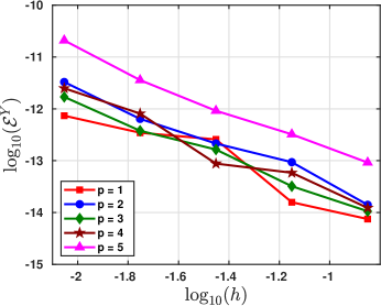
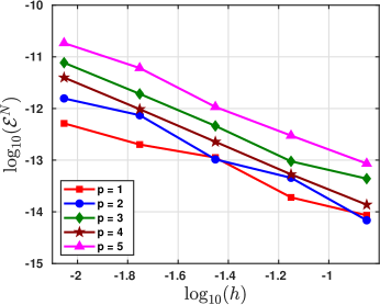
Figure 2: $h$-dependence of the errors in (5.1) for the patch tests with solution $u_{p}$ in (5.2).

5.1.2 Smooth solution

On the space-time domain $Q_{T}=(0,1)\times(0,1)$, we consider the problem with exact smooth solution

$$u(x,t)=\sin(t)\sin(3\pi x).$$ (5.3)

In Figure 3, we show the rates of convergence of the errors in (5.1) obtained using a sequence of meshes with $h_{K_{\mathbf{x}}}=h_{I_{n}}=0.2\times 2^{-i}$, for $i=1,\ldots,5$, and different approximation degrees $p$. We observe convergence of order $\mathcal{O}(h^{p})$ for the error $\mathcal{E}^{Y}$, of order $\mathcal{O}(h^{p+\frac{1}{2}})$ for the error $\mathcal{E}^{U}$, and of order $\mathcal{O}(h^{p+1})$ for the errors $\mathcal{E}^{N}$ and $\mathcal{E}^{L}$. Such rates of convergence are in agreement with estimate (4.7) and the approximation rates that might be expected from the norms in (5.1).

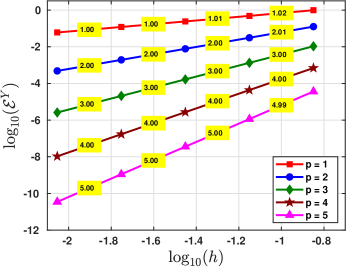
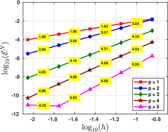
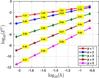
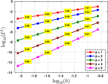
Figure 3: $h$-convergence of the errors in (5.1) for the test case with smooth solution (5.3). The numbers in the yellow rectangles denote the experimental orders of convergence.

5.1.3 Singular solutions

We assess the convergence of the method for solutions with finite Sobolev regularity. We use same sequence of meshes as in Subsection 5.1.1. For $Q_{T}=(0,1)\times(0,1)$ and $\alpha>-1/2$, we consider the singular solutions

$$u_{\alpha}(x,t)=t^{\alpha}\sin(\pi x).$$ (5.4)

We have that $u_{\alpha}$ and $\partial_{x}u_{\alpha}$ belong to $H^{\alpha+1/2-\epsilon}(0,1;\mathcal{C}^{\infty}(0,1))$ for any $\epsilon>0$. The singularity occurs at the initial time. The errors in (5.1) are depicted in Figures 4 and 5 for $\alpha=0.55$ and $\alpha=0.75$. We observe convergence of order $\mathcal{O}\left(h^{\min\{p,\alpha+1/2\}}\right)$ for the error $\mathcal{E}^{Y}$, of order $\mathcal{O}(h^{\alpha-\frac{1}{2}})$ for the error $\mathcal{E}^{N}$, of order $\mathcal{O}(h^{\alpha})$ for the error $\mathcal{E}^{U}$, and of order $\mathcal{O}(h^{\alpha+\frac{1}{2}})$ for the error $\mathcal{E}^{L}$.

For a continuous finite element discretization of formulation (1.4), lower rates of convergence are obtained; see [11, Sect. 7.5.3].

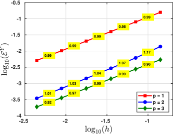
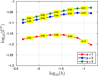
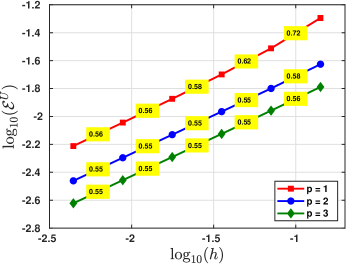
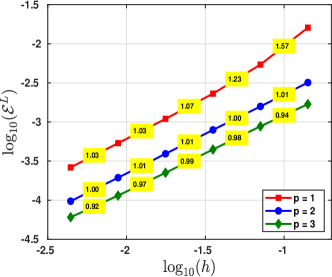
Figure 4: $h$-convergence of the errors in (5.1) for the test case with

singular solution $u_{\alpha}$ (5.4) with $\alpha=0.55$.

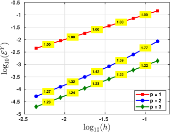
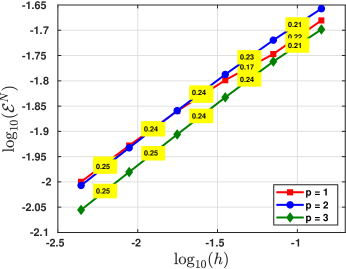
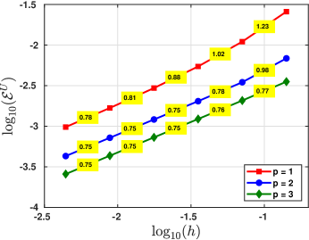
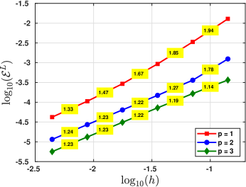
Figure 5: $h$-convergence of the errors in (5.1) for the test case with singular solution $u_{\alpha}$ (5.4) with $\alpha=0.75$.

5.1.4 Incompatible initial and boundary conditions

On the space-time domain $Q_{T}=(0,1)\times(0,1)$, we consider the heat equation problem (1.1) with zero source term $(f=0)$, homogeneous Dirichlet boundary conditions ($u=0$ on $\partial\Omega\times(0,T)$), and constant initial condition ($u=1$ on $\Omega\times\{0\}$). The corresponding exact solution is given by the Fourier series

$$u(x,t)=\sum_{n=0}^{\infty}\frac{4}{(2n+1)\pi}\sin\left((2n+1)\pi x\right)\exp\left(-(2n+1)^{2}\pi^{2}t\right).$$ (5.5)

Due to the incompatibility of the initial and boundary conditions, $u$ is discontinuous at $(0,0)$ and $(1,0)$, and does not belong to $H^{1}(Q_{T})$ but belongs to $H^{s}\left(0,1;H^{1}_{0}(0,1)\right)$ for any $s<1/4$; see [16, Sect. 7.1]. Therefore, the rates of convergence obtained cannot be predicted by Theorem 4.4.

In Figure 6, we show the errors obtained with $p=1,2$ on a sequence of uniform Cartesian meshes for the proposed VEM and on a sequence of structured triangular meshes for the continuous finite element method in [18]. The continuous finite element method does not converge in the $Y$-norm, while the error $\mathcal{E}^{Y}$ of the proposed VEM converges with order $\mathcal{O}(h^{1/4})$. For the computation of the error, we truncate the series (5.5) at $n=250$.

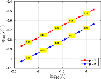
(a)

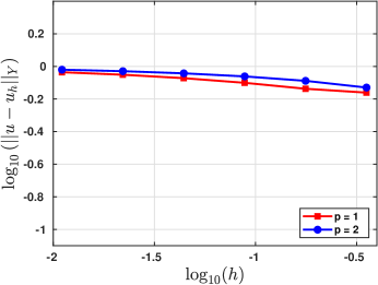
(b)

Figure 6: $h$-convergence for the test case with exact solution (5.5) with incompatible initial and boundary conditions.

5.1.5 Increasing the degree of approximation

We are also interested in the performance of the $p$-version of the method, i.e., we fix a mesh and increase the degree of approximation. This is worth investigating also in view of the design of $hp$ refinements. We consider the smooth solution test case from Figure 5.1.2 with a fixed mesh with $h_{I_{n}}=h_{K_{\mathbf{x}}}=0.1$. The results shown in Figure 7 in semilogy scale. We observe the expected exponential convergence in terms of the square root of $N_{DoFs}$ for all the VEM errors.

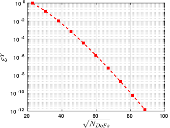
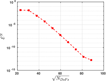
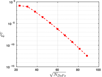
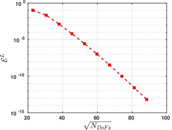
Figure 7: $p$-convergence of the errors in (5.1) for the test case with smooth solution in (5.3).

5.2 Results in (2+1)-dimension

We use tensor-product-in-time meshes and uniform partitions of the time interval $(0,T)$, and discretize the spatial domain $\Omega$ with sequences of quadrilateral meshes such as that in Figure 8 (left panel). We checked that the method passes the patch test also in the (2+1) dimensional case. We do not report the results for the sake of brevity.

On $Q_{T}=(0,1)^{2}\times(0,1)$, we consider

$$u(\mathbf{x},t)=\exp(-t)\sin(\pi x_{1})\sin(\pi x_{2}).$$ (5.6)

In Figure 8 (right panel), we display the rates of convergence using different values of $p$ and observe the expected rates of convergence for the error $\mathcal{E}^{Y}$.

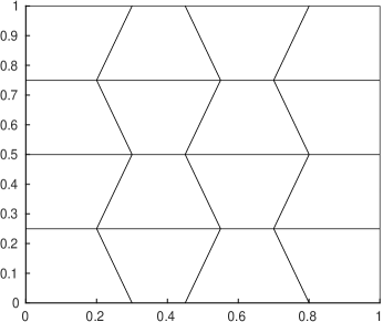
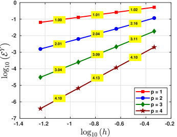
Figure 8: Left panel: example of mesh for the 2-dimensional spatial domain used in the numerical experiments. Right panel: $h$-convergence for the test case with smooth solution (5.6).

6 Conclusions

We designed and analyzed a space-time virtual element method for the heat equation based on a standard Petrov-Galerkin variational formulation. The advantages of using the proposed space-time VEM over standard space-time finite element methods are that it allows for decomposing the linear system stemming from the method into smaller systems associated with different time slabs; can be modified into a Trefftz variant; permits the treatment of incompatible initial and boundary data. We proved well posedness of the method and optimal a priori error estimates. Numerical results validate the expected rates of convergence.

In [12], the method introduced in this paper has been extended to more general prismatic meshes with hanging facets and variable degrees of accuracy, enabling the implementation of $hp$-adaptive mesh refinements. Tests of an adaptive procedure driven by a residual-type error indicator are also presented there.

References

- [1] R. Andreev. Stability of sparse space-time finite element discretizations of linear parabolic evolution equations. IMA J. Numer. Anal., 33(1):242–260, 2013.
- [2] B. P. Ayuso de Dios, K. Lipnikov, and G. Manzini. The nonconforming virtual element method. ESAIM Math. Model. Numer. Anal., 50(3):879–904, 2016.
- [3] L. Beirão da Veiga, F. Brezzi, A. Cangiani, G. Manzini, L.D. Marini, and A. Russo. Basic principles of virtual element methods. Math. Models Methods Appl. Sci., 23(01):199–214, 2013.
- [4] P. B. Bochev and M. D. Gunzburger. Least-squares finite element methods, volume 166 of Applied Mathematical Sciences. Springer, New York, 2009.
- [5] S. C. Brenner. Poincaré–Friedrichs inequalities for piecewise functions. SIAM J. Numer. Anal., 41(1):306–324, 2003.
- [6] A. Cangiani, Z. Dong, and E. H. Georgoulis. -version space-time discontinuous Galerkin methods for parabolic problems on prismatic meshes. SIAM J. Sci. Comput., 39(4):A1251–A1279, 2017.
- [7] R. Dautray and J.-L. Lions. Mathematical Analysis and Numerical Methods for Science and Technology, volume 5, Evolution Problems I. Springer-Verlag, 1992.
- [8] T. Führer and M. Karkulik. Space-time least-squares finite elements for parabolic equations. Comput. Math. Appl., 92:27–36, 2021.
- [9] G. Gantner and R. Stevenson. Further results on a space-time FOSLS formulation of parabolic PDEs. ESAIM Math. Model. Numer. Anal., 55(1):283–299, 2021.
- [10] G. Gantner and R. Stevenson. Improved rates for a space-time FOSLS of parabolic PDEs. 2022.
- [11] S. Gómez. Nonconforming space–time methods for evolution PDEs. PhD thesis, University of Pavia, in preparation, 2023.
- [12] S. Gómez, L. Mascotto, and I Perugia. Design and performance of a space-time virtual element method for the heat equation on prismatic meshes. https://arxiv.org/abs/2306.09191, 2023.
- [13] U. Langer and O. Steinbach. Space-Time Methods: Applications to Partial Differential Equations, volume 25. Walter de Gruyter GmbH & Co KG, 2019.
- [14] J.-L. Lions and E. Magenes. Non-homogeneous boundary value problems and applications. Vol. I. Die Grundlehren der mathematischen Wissenschaften, Band 181. Springer-Verlag, New York-Heidelberg, 1972.
- [15] M. Neumüller. Space-Time Methods: Fast Solvers and Applications. PhD thesis, TU Graz, 2013.
- [16] D. Schötzau and Ch. Schwab. Time discretization of parabolic problems by the -version of the discontinuous Galerkin finite element method. SIAM J. Numer. Anal., 38(3):837–875, 2000.
- [17] Ch. Schwab and R. Stevenson. Space-time adaptive wavelet methods for parabolic evolution problems. Math. Comp., 78(267):1293–1318, 2009.
- [18] O. Steinbach. Space-time finite element methods for parabolic problems. Comput. Methods Appl. Math., 15(4):551–566, 2015.
- [19] O. Steinbach and M. Zank. Coercive space-time finite element methods for initial boundary value problems. Electron. Trans. Numer. Anal., 52:154–194, 2020.
- [20] R. Stevenson and J. Westerdiep. Minimal residual space-time discretizations of parabolic equations: asymmetric spatial operators. Comput. Math. Appl., 101:107–118, 2021.
- [21] G. Vacca and L. Beirão da Veiga. Virtual element methods for parabolic problems on polygonal meshes. Numer. Methods Partial Differential Equations, 31(6):2110–2134, 2015.
- [22] J. Wloka. Partial differential equations. Cambridge University Press, Cambridge, 1987.