Targeted Adversarial Attacks on Deep Reinforcement Learning Policies via Model Checking

Abstract

Deep Reinforcement Learning (RL) agents are susceptible to adversarial noise in their observations that can mislead their policies and decrease their performance. However, an adversary may be interested not only in decreasing the reward, but also in modifying specific temporal logic properties of the policy. This paper presents a metric that measures the exact impact of adversarial attacks against such properties. We use this metric to craft optimal adversarial attacks. Furthermore, we introduce a model checking method that allows us to verify the robustness of RL policies against adversarial attacks. Our empirical analysis confirms (1) the quality of our metric to craft adversarial attacks against temporal logic properties, and (2) that we are able to concisely assess a system’s robustness against attacks.

1 INTRODUCTION

Deep reinforcement learning (RL) has changed how we build agents for sequential decision-making problems (Mnih et al.,, 2015; Levine et al.,, 2016). It has triggered applications in critical domains like energy, transportation, and defense (Farazi et al.,, 2021; Nakabi and Toivanen,, 2021; Boron and Darken,, 2020). An RL agent learns a near-optimal policy (based on a given objective) by making observations and gaining rewards through interacting with the environment (Sutton and Barto,, 2018). Despite the success of RL, potential security risks limit its usage in real-life applications. The so-called adversarial attacks introduce noise into the observations and mislead the RL decision-making to drop the cumulative reward, which may lead to unsafe behaviour (Huang et al., 2017a, ; Chen et al.,, 2019; Ilahi et al.,, 2022; Moos et al.,, 2022; Amodei et al.,, 2016).

Generally, rewards lack the expressiveness to encode complex safety requirements (Vamplew et al.,, 2022; Hasanbeig et al.,, 2020). Therefore, for an adversary, capturing how much the cumulative reward is reduced may be too generic for attacks targeting specific safety requirements. For instance, an RL taxi agent may be optimized to transport passengers to their destinations. With the already existing adversarial attacks, the attacker can prevent the agent from transporting the passenger. However, the attacker cannot create controlled adversarial attacks that may increase the probability that the passenger never gets picked up or that the passenger gets picked up but never arrives at its destination. More generally, current adversary attacks are not able to control temporal logic properties.

This paper aims to combine adversarial RL with rigorous model checking (Baier and Katoen,, 2008), which allows the adversary to create so-called property impact attacks (PIAs) that can influence specific RL policy properties. These PIAs are not limited by properties that can be expressed by rewards (Littman et al.,, 2017; Hahn et al.,, 2019; Hasanbeig et al.,, 2020; Vamplew et al.,, 2022), but support a broader range of properties that can be expressed by probabilistic computation tree logic (PCTL; Hansson and Jonsson,, 1994). Our experiments show that for PCTL properties, it is possible to create targeted adversarial attacks that influence them specifically. Furthermore, the combination of model checking and adversarial RL allows us to verify via permissive policies (Dräger et al.,, 2015) how vulnerable trained policies are against PIAs. Our main contributions are:

• a metric to measure the impact of adversarial attacks on a broad range of RL policy properties,

• a property impact attack (PIA) to target specific properties of a trained RL policy, and

• a method that checks the robustness of RL policies against adversarial attacks.

The empirical analysis shows that the method to attack RL policies can effectively modify PCTL properties. Furthermore, the results support the theoretical claim that it is possible to model check the robustness of RL policies against property impact attacks.

The paper is structured in the following way. First, we summarize the related work and position our paper in it. Second, we explain the fundamentals of our technique. Then, we present the adversarial attack setting, define our property impact attack, and show a way to model check policy robustness against such adversarial attacks. After that, we evaluate our methods in multiple environments.

2 RELATED WORK

We now summarize the related work and position our paper in between adversarial RL and model checking.

There exist a variety of adversarial attack methods to attack RL policies with the goal of dropping their total expected reward (Chan et al.,, 2020; Lin et al., 2017b, ; Ilahi et al.,, 2022; Lin et al., 2017a, ; Clark et al.,, 2018; Yu and Sun,, 2022). The first proposed adversarial attack on deep RL policies (Huang et al., 2017a, ) uses a modified version of the fast gradient sign method (FGSM), developed by Goodfellow et al., (2015), to force the RL policy to make malicious decisions (for more details, see Section 3.2). However, none of the previous work let the attacker target temporal logic properties of RL policies. Chan et al., (2020) create more effective attacks that modify only one feature (if the smallest sliding window is used) of the observation of the agent, their approach empirically measures the impact of each feature in the reward, then it modifies the feature with the highest impact. We build upon this idea and measure the impact of changing each feature in a given temporal logic property instead of the reward.

There exist a large body of work that combines RL with model checking (Wang et al.,, 2020; Hasanbeig et al.,, 2020; Hahn et al.,, 2019; Hasanbeig et al.,, 2019; Fulton and Platzer,, 2019; Sadigh et al.,, 2014; Bouton et al.,, 2019; Chatterjee et al.,, 2017) but no work that uses model checking to create adversarial attacks for RL policies (Chen et al.,, 2019; Ilahi et al.,, 2022; Moos et al.,, 2022). Most work about the formal robustness checking of deep learning models focuses on supervised learning (Katz et al.,, 2017, 2019; Gehr et al.,, 2018; Huang et al., 2017b, ; Ruan et al.,, 2018). In the RL setting, Zhang et al., (2020) introduce a formal approach to check the robustness against adversarial attacks with respect to the reward. They formulate the perturbation on state observations as a modified Markov decision process (MDP). Furthermore, they can obtain certain robustness certificates under attack. For environments like Pong, they can guarantee actions do not change for all frames during policy execution, thus guaranteeing the cumulative rewards under attack. We, on the other hand, focus on the robustness of temporal PCTL properties against attacks.

3 BACKGROUND

In this section, we introduce the necessary foundations. First, we summarize the modeling and analysis of probabilistic systems. Second, we introduce a method to attack deep RL policies and a method that increases the robustness of trained RL policies.

3.1 Probabilistic Systems

A probability distribution over a set $X$ is a function $\mu:X\rightarrow[0,1]$ with $\sum_{x\in X}\mu(x)=1$. The set of all distributions over $X$ is denoted by $Distr(X)$.

Definition 3.1 (Markov Decision Process).

A Markov decision process (MDP) is a tuple $M=(S,s_{0},Act,T,rew)$ where $S$ is a finite, nonempty set of states, $s_{0}\in S$ is an initial state, $Act$ is a finite set of actions, $T\colon S\times Act\rightarrow Distr(S)$ is a probability transition function. We employ a factored state representation $S\subseteq\mathbb{Z}^{n}$, where each state $s\in\mathbb{Z}^{n}$ is an $n$-dimensional vector of features $(f_{1},f_{2},...,f_{n})$ such that $f_{i}\in\mathbb{Z}$ for $1\leq i\leq n$. We define $rew\colon S\times Act\rightarrow\mathbb{R}$ as a reward function.

The available actions in $s\in S$ are $Act(s)=\{a\in Act\mid T(s,a)\neq\bot\}$. An MDP with only one action per state ($\forall s\in S\colon|Act(s)|=1$) is a discrete-time Markov chain (DTMC). Note that features do not necessarily have to have the same domain size. We define $\mathcal{F}$ as the set of all features $f_{i}$ in state $s\in S$.

A path of an MDP $M$ is an (in)finite sequence $\tau=s_{0}\xrightarrow[\text{}]{\text{$a_{0},r_{0}$}}s_{1}\xrightarrow[\text{}]{\text{$a_{1},r_{1}$}}...$, where $s_{i}\in S$, $a_{i}\in Act(s_{i})$, $r_{i}\vcentcolon=rew(s_{i},a_{i})$, and $T(s_{i},a_{i})(s_{i+1})\neq 0$. A state $s^{\prime}$ is reachable from state $s$ if there exists a path $\tau$ from state $s$ to state $s^{\prime}$. We say a state $s$ is reachable if $s$ is reachable from $s_{0}$.

Definition 3.2 (Policy).

A memoryless deterministic policy for an MDP $M{=}(S,s_{0},Act,T,rew)$ is a function $\pi\colon S\rightarrow Act$ that maps a state $s\in S$ to an action $a\in Act(s)$.

Applying a policy $\pi$ to an MDP $M$ yields an induced DTMC, denoted as $D$, where all non-determinism is resolved. This way, we say a state $s$ is reachable by a policy $\pi$ if $s$ is reachable in the DTMC induced by $\pi$. $\Lambda$ is the set of all possible memoryless policies.

To analyze the properties of an induced DTMC, it is necessary to specify the properties via a specification language like probabilistic computation tree logic PCTL (Hansson and Jonsson,, 1994).

Definition 3.3 (PCTL Syntax).

Let $AP$ be a set of atomic propositions. The following grammar defines a state formula: $\Phi\coloneqq\text{ true }|\text{ a }|\text{ }\Phi_{1}\land\Phi_{2}\text{ }|\text{ }\lnot\Phi\text{ }|P_{\bowtie p}|P^{max}_{\bowtie p}(\phi)\text{ }|\text{ }P^{min}_{\bowtie p}(\phi)$ where $a\in AP,\bowtie\in\{<,>,\leq,\geq\}$, $p\in[0,1]$ is a threshold, and $\phi$ is a path formula which is formed according to the following grammar $\phi\coloneqq X\Phi\text{ }|\text{ }\phi_{1}\text{ }U\text{ }\phi_{2}\text{ }|\text{ }\phi_{1}\text{ }F_{\theta t}\text{ }\phi_{2}\text{ }|G\text{ }\Phi$ with $\theta=\{<,\leq\}$.

PCTL formulae are interpreted over the states of an induced DTMC. In a slight abuse of notation, we use PCTL state formulas to denote probability values. That is, we sometimes write $P_{\bowtie p}(\phi)$ where we omit the threshold $p$. For instance, $P(F_{\leq 100}collision)$ denotes the reachability probability of eventually running into a collision within the first $100$ time steps.

There is a variety of model checking algorithms for verifying PCTL properties (Courcoubetis and Yannakakis,, 1988, 1995), and PRISM and Storm offer efficient and mature tool support (Kwiatkowska et al.,, 2011; Hensel et al.,, 2022). COOL-MC (Gross et al.,, 2022) allows model checking of a trained RL policy against a PCTL property and MDP. The tool builds the induced DTMC on the fly via an incremental building process (Cassez et al.,, 2005; David et al.,, 2015).

3.2 Adversarial Attacks on Deep RL Policies

The standard learning goal for RL is to find a policy $\pi$ in a MDP such that $\pi$ maximizes the expected accumulated discounted rewards, that is, $\mathbb{E}[\sum^{L}_{t=0}\gamma^{t}R_{t}]$, where $\gamma$ with $0\leq\gamma\leq 1$ is the discount factor, $R_{t}$ is the reward at time $t$, and $L$ is the total number of steps. Deep RL uses neural networks to train policies. A neural network is a function parameterized by weights $\theta$. In deep RL, the policy $\pi$ is encoded using a neural network which can be trained by minimizing a sequence of loss functions $J(\theta,s,a)$ (Mnih et al.,, 2013).

An adversary is a malicious actor that seeks to harm or undermine the performance of an RL system. For instance, an adversary may try to decrease the expected discounted reward by attacking the RL policy via adversarial attacks.

Definition 3.4 (Adversarial Attack).

An adversarial attack $\delta\colon S\rightarrow S$ maps a state $s$ to an adversarial state $s_{adv}$ (see Figure 1). A successful adversarial attack at a given state $s$ leads to a misjudgment of the RL policy ($\pi(s)~{}\neq~{}\pi(\delta(s))$) and an attack is $\epsilon$-bounded if $\lVert\delta(s)-s\rVert_{\infty}\leq\epsilon$ with $l_{\infty}$-norm defined as $\lVert\delta(s)-s\rVert_{\infty}=max_{\delta_{i}\in\delta}|\delta_{i}-s_{i}|$.

Recall that states are $n$-dimensional vectors of features from $\mathbb{Z}^{n}$. Executing a policy $\pi$ on an MDP $M$ and attacking the policy $\pi$ at each reachable state $s$ by $\delta$ yields an adversarial-induced DTMC $D_{adv}$. There exist a variety of adversarial attack methods to create adversarial attacks $\delta$ (Ilahi et al.,, 2022; Gleave et al.,, 2020; Lee et al.,, 2020, 2021; Rakhsha et al.,, 2020; Carlini and Wagner,, 2017).

(a) RL policy interaction with the environment.

(b) An adversary manipulates with $\delta$ the observations of the RL policy $\pi$ and its interaction with the environment.

Figure 1: RL (a) vs. adversarial RL (b).

Our work builds upon the FGSM attack and the work of Chan et al., (2020). Given the weights $\theta$ of the neural network policy $\pi$ and a loss $J(\theta,s,a)$ with state $s$ and $a\coloneqq\pi(s)$, the FGSM, denoted as $\delta_{\text{FGSM}}\colon S\rightarrow S$, adds noise whose direction is the same as the gradient of the loss $J(\theta,s,a)$ w.r.t the state $s$ to the state $s$ (Huang et al., 2017a, ) and the noise is scaled by $\epsilon\in\mathbb{Z}$ (see Equation 1). Note that we are dealing with integer $\epsilon$-values because our states are comprised of integer features. We specify the $\bigtriangledown$-operator as a vector differential operator. Depending on the gradient, we either add or subtract $\epsilon$.

$$\delta_{\text{FGSM}}(s)=s+\epsilon\cdot sign(\bigtriangledown_{s}J(\theta,s,a))$$ (1)

A FGSM for feature $f_{i}$, denoted as $\delta_{\text{FGSM}}^{(f_{i})}(s)$, modifies only the feature $f_{i}$ in state $s$.

$$\delta_{\text{FGSM}}^{(f_{i})}(s)=s+\epsilon\cdot sign(\bigtriangledown_{s_{f_{i}}}J(\theta,s,a))$$ (2)

We denote the set of all possible $\epsilon$-bounded attacks at state $s$ via feature $f_{i}$, including $\delta^{(f_{i})}(s)=s$ for no attack, as $\Delta^{(f_{i})}_{\epsilon}(s)$.

Chan et al., (2020) first generate for all features a static reward impact (SRI) map by attacking each feature (in the case of the smallest sliding window) with the FGSM attack to measure its impact (the drop of the expected reward) offline. A feature $f_{i}$ with a more significant impact indicates that changing this feature $f_{i}$ via $\delta_{\text{FGSM}}^{(f_{i})}$ will influence the expected discounted reward more than via another feature $f_{k}$ with a less significant impact. For each feature $f_{i}$, this is done multiple times $N$, where each iteration executes the RL policy on the environment and attacks at every state the feature $f_{i}$ via the FGSM attack $\delta_{\text{FGSM}}^{(f_{i})}$. After calculating the SRI, they use all the SRI values of the features $f_{i}$ to select the most vulnerable feature to attack the deployed RL policy.

Adversarial training retrains the already trained RL policy by using adversarial attacks during training (see Figure 1(b)) to increase the RL policy robustness (Pinto et al.,, 2017; Liu et al.,, 2022; Korkmaz, 2021b, ).

4 METHODOLOGY

We introduce the general adversarial setting, the property impact (PI), the property impact attack (PIA), and bounded robustness.

4.1 Attack Setting

We first describe our method’s adversarial attack setting (adversary’s goals, knowledge, and capabilities).

Goal. The adversary aims to modify the property value of the target RL policy $\pi$ in its environment (modeled as an MDP). For instance, the adversary may try to increase the probability that the agent collides with another object (i.e. $\max_{\delta}P(F\text{ }\mathit{collision})$ in the adversarial-induced DTMC).

Knowledge. The adversary that knows the weights $\theta$ of the trained policy (for the FGSM attack) and knows the MDP of the environment. Note that we can replace the FGSM attack with any other attack. Therefore, knowing the weights of the trained policy should not be a strict constraint.

Capabilities. The adversary can attack the trained policy $\pi$ at every visited state $s$ during the incremental building process for the model checking of the adversarial-induced DTMC and after the RL policy got deployed.

4.2 Property Impact Attack (PIA)

Combining adversarial RL with model checking allows us to craft adversarial property impact attacks (PIAs) that target temporal logic properties. Our work builds upon the research of Chan et al., (2020). Instead of calculating SRIs (see Section 3.2), we calculate property impacts (PIs). The PI values are used to select the feature $f_{i}$ with the most significant $PI$-value to attack the deployed RL policy in its environment ($f_{i}=\operatorname*{argmax}_{f_{i}\in\mathcal{F}}PI(\pi,P(\phi),f_{i},\epsilon)$).

Definition 4.1 (Property Impact).

The property impact $PI\colon\Lambda\times\Theta\times\mathcal{F}\times\mathbb{Q}\rightarrow\mathbb{Q}$ quantifies the impact of an adversarial attack $\delta_{\text{FGSM}}^{(f_{i})}\in\Delta^{(f_{i})}_{\epsilon}(s)$ via a feature $f_{i}\in\mathcal{F}$ on a given RL policy property $P(\phi)\in\Theta$ with $\Theta$ as the set of all possible PCTL properties for the MDP $M$.

A feature $f_{i}$ with a more significant PI-value indicates that changing this feature $f_{i}$ via $\delta_{\text{FGSM}}^{(f_{i})}$ will influence the property (expressed by the property query $P(\phi)$) more than via another feature $f_{k}$ with a less significant PI-value.

Algorithm 1 Calculate the property impact (PI) for a given MDP $M$, policy $\pi$, property query $P(\phi)$, feature $f_{i}$, and FGSM attack strength $\epsilon$.

1:procedure PI($\pi,P(\phi),f_{i},\epsilon$)

2:     $r\leftarrow property\_result(M,\pi,P(\phi))$

3:     $r_{adv}\leftarrow adv\_property\_result(M,\pi,P(\phi),f_{i},\epsilon)$

4:     return $|r-r_{adv}|$

5:end procedure

In Algorithm 1, we explain how to calculate the PI-value for a given MDP $M$, policy $\pi$, PCTL property query $P(\phi)$, feature $f_{i}$, and FGSM attack $\delta_{\text{FGSM}}^{(f_{i})}$. First, we incrementally build the induced DTMC of the policy $\pi$ and the MDP $M$ to check the property value $r$ of the policy $\pi$ via the function property_result. The function property_result uses COOL-MC and inputs the MDP $M$, policy $\pi$, and PCTL property query $P(\phi)$ into it to calculate the probability $r$. Second, we incrementally build the adversarial-induced DTMC $D_{adv}$ of the policy $\pi$ and the MDP $M$ with the $\epsilon$-bounded FGSM attack $\delta_{\text{FGSM}}^{(f_{i})}$ to check its probability $r_{adv}$ via the function $adv\_property\_result$. To support the building and model checking of adversarial-induced DTMCs via $adv\_property\_result$, we extend the incremental building process of COOL-MC in the following way. For every reachable state $s$ by the policy $\pi$, the policy $\pi$ is queried for an action $a=\pi(s)$. In the underlying MDP, only states $s$ that may be reached via that action $a$ are expanded. The resulting model is fully probabilistic, as no action choices are left open. It is, in fact, the Markov chain induced by the original MDP $M$ and the policy $\pi$. An adversary can now inject adversarial attacks $\delta(s)$ at every state $s$ that gets passed to the policy $\pi$ during the incrementally building process (Zhang et al.,, 2020). This may lead to the effect that the policy $\pi$ makes a misjudgment $(\pi(s)\neq\pi(\delta(s))$ and results into an adversarial-induced DTMC $D_{adv}$. This allows us to model check the adversarial-induced DTMCs $D_{adv}$ to gain the adversarial probability $r_{adv}$. Finally, we measure the property impact value by measuring the absolute difference between $r$ and $r_{adv}$.

Figure 2: ($\epsilon,\alpha$)-robustness checking for an MDP with the state set $S=\{x\in[0,4]\}$, action set $Act=\{a,b.c\}$, trained policy $\pi$, adversarial attack strength $\epsilon=1$ ($\Delta_{\epsilon=1}(s)=\{s+1,s-1,s\}$), and property $P(F\text{ }x=2)=0$ (for original blue policy $\pi$). The blue induced DTMC is the original one, and the MDP (blue and red) is the adversarial MDP representing the permissive policy $\Omega$. For the permissive policy $\Omega$, we get $P^{max}(F\text{ }x=2)=1$ which results in a $P^{max}(F\text{ }x=2)-P(Fx=2)=1$ and indicate that $\pi$ is not robust for, for example, $\alpha=0$ and $\epsilon=1$. We can extract the optimal attack set $\{\delta(s)=s+1\text{ at state }x=1\}$.

4.3 RL Policy Robustness

A trained RL policy $\pi$ can be robust against an $\epsilon$-bounded PIA that attacks a temporal logic property $P(\phi)$ via feature $f_{i}$ ($PI(\pi,P(\phi),f_{i},\epsilon)=0$). However, this is a weak statement about robustness since there still exist multiple adversarial attacks $\delta^{(f_{i})}(s)$ with $\lVert\delta^{(f_{i})}(s)-s\rVert_{\infty}\leq\epsilon$ generated by other attacks, such as the method from Carlini and Wagner, (2017).

Given a fixed policy $\pi$ and a set of attacks $\Delta^{(f_{i})}_{\epsilon}(s)$, we generate a permissive policy $\Omega$. Applying this policy $\pi$ in the original MDP $M$ generates a new MDP $M^{\prime}$ that describes all potential behavior of the agent under the attack.

Definition 4.2 (Behavior under attack).

A permissive policy $\Omega\colon S\rightarrow 2^{\textsf{Act}}$ selects, at every state $s$, all actions that can be queried via $\Delta^{(f_{i})}_{s}(s)$. We consider $\Omega(s)=\bigcup_{\delta^{(f_{i})}_{i}\in\Delta^{(f_{i})}_{s}(s)}\pi(\delta^{(f_{i})}_{i}(s))$ with $\pi(\delta^{(f_{i})}_{i}(s))\in Act(s)$.

Applying a permissive policy to an MDP does not necessarily resolve all nondeterminism, since more than one action may be selected in some state(s). The induced model is then (again) an MDP. We are able to apply model checking, which typically results in best- and worst-case probability bounds $P^{max}(\phi)$ and $P^{min}(\phi)$ for a given property query $P(\phi)$.

We use the induced MDP to model check the robustness (see Definition 4.3) against every possible $\epsilon$-bounded attack $\delta^{(f_{i})}(s)$ for a trained RL policy $\pi$ in its environment and bound the robustness to an $\alpha$-threshold (property impacts below a given threshold $\alpha$ may be acceptable).

Definition 4.3 (Bounded robustness).

A policy $\pi$ is called robustly bounded by $\epsilon$ and $\alpha$ ($\epsilon,\alpha$-robust) for property query $\phi$ if it holds that

$$|P^{*}(\phi)-P(\phi)|\leq\alpha$$ (3)

for all possible $\epsilon$-bounded adversarial attacks $\Delta^{(f_{i})}_{\epsilon}(s)$ at every reachable state $s$ by the permissive policy $\Omega$. We define $\alpha\in\mathbb{Q}$ as a threshold (in this paper, we focus on probabilities and therefore $\alpha\in[0,1]$). $|P^{*}(\phi)-P(\phi)|$ stands for the largest impact of a possible attack. We denote $P^{*}$ as $P^{max}$ or $P^{min}$ depending if the attack should increase ($P^{max}$) or decrease ($P^{min}$) the probability.

By model checking the robustness of the trained RL policies (see Figure 2), it is possible to extract for each state $s$ the adversarial attack $\delta^{(f_{i})}$ that is part of the most impactful attack and use the corresponding attack as soon as the state gets observed by the adversary. This is possible because the underlying model of the induced MDP allows the extraction of the state and action pairs ($s,a_{adv}$) that lead to the wanted property value modification ($a_{adv}\coloneqq\pi(\delta^{(f_{i})}(s))$).

5 EXPERIMENTS

We now evaluate our PI method, property impact attack (PIA), and robustness checker method in multiple environments. The experiments are performed by initially training the RL policies using the deep Q-learning algorithm (Mnih et al.,, 2013), then using the trained policies to answer our research questions. First, we compare our PI-method with the SRI-method (Chan et al.,, 2020). Second, we use PIAs to attack policy properties. Third, we discuss the limitations of PIAs. Last but not least, we show that it is possible to make trained policies more robust against PIAs by using adversarial training.

5.1 Setup

We now explain the setup of our experiments.

Environments. We used our proposed methods in a variety of environments (see Figure 3, Figure 5, and Table 2). We use the Freeway (for a fair comparison between the SRI and PI method) and the Taxi. Additionally, we use the environments Collision Avoidance, Stock Market, and Smart Grid (see Appendix A for more details).

Freeway is an action video game for the Atari 2600. A player controls a chicken (up, down, no operation) who must run across a highway filled with traffic to get to the other side. Every time the chicken gets across the highway, it earns a reward of one. An episode ends if the chicken gets hit by a car or reaches the other side. Each state is an image of the game’s state. Note that we use an abstraction of the original game (see Figure 3), which sets the chicken into the middle column of the screen and contains fewer pixels than the original game, but uses the same reward function and actions.

The taxi agent has to pick up passengers and transport them to their destination without running out of fuel. The environment terminates as soon as the taxi agent does the predefined number of jobs or runs out of fuel. After the job is done, a new guest spawns randomly at one of the predefined locations. We define the maximal taxi fuel level as ten and the maximal number of jobs as two. To refuel the taxi, the agent needs to drive to the gas station cell ($x=1,y=2$). The problem is formalized as follows:

$$S =\{(x,y,Xloc,Yloc,Xdest,Ydest,$$

$$\qquad\qquad fuel,done,pass,jobs,done),...\}$$

$$Act =\{north,east,south,west,pick\_up,drop\}$$

$$rew =\begin{cases}0\text{, if passenger successfully dropped.}\\ 21\text{, if passenger got picked up.}\\ 21+|x-Xdest|+\\ \quad|y-Ydest|\text{, if passenger on board.}\\ 21+|x-Xloc|+|y-Yloc|\text{, otherwise.}\end{cases}$$

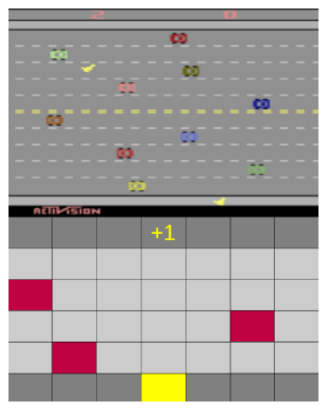
Figure 3: A comparison between the Atari 2600 Freeway game (top) and our abstracted version (bottom).

Properties. Table 1 presents the property queries of the policy trained by an RL agent achieves in these properties without the attack ($=$). For example, $pass\_empty$ describes the probability of the taxi agent running out of fuel while having a passenger on board, which is $0$ for the policy without an attack.

Trained RL policies. We trained deep Q-learning policies for the environments. See Appendix B for a more detailed description of the RL training.

Env.	Label	PCTL Property Query ($P(\phi)$)	$=$
Fr	crossed	$P(F\text{ }crossed)$	$1.0$
Taxi	deadlock1	$P(fuel\geq 4\text{ }U\text{ }(G(jobs=1\land\lnot empty\text{ }\land pass)))$	$0.0$
	deadlock2	$P(fuel\geq 4\text{ }U\text{ }(G(jobs=1\land\lnot empty\land\lnot pass)))$	$0.0$
	station_empty	$P((((jobs{=}0$ $U$ $x{=}1\land y{=}2)$ $U$ $(jobs{=}0\land\lnot(x{=}1\land y{=}2)))$ $U$ $empty\land jobs{=}0))$	$0.0$
	$\overline{\textrm{station}}$_empty	$P(F\text{ }(empty\land jobs=0)\land G\lnot(x\neq 1\land y\neq 2))$	$0.0$
	pass_empty	$P(F\text{ }(empty\land pass))$	$0.0$
	$\overline{\textrm{pass}}$_empty	$P(F\text{ }(empty\land\lnot pass))$	$0.0$
Coll.	collision	$P(F_{\leq 100}\text{ }collision)$	$0.1$
SG	blackout	$P(F_{\leq 100}\text{ }blackout)$	$0.2$
SM	bankruptcy	$P(F\text{ }bankruptcy)$	$0.0$

Table 1: PCTL property queries, with their labels and the original result of the property query without an attack ($=$). $Fr$ stands for Freeway, $Coll.$ stands for Collision Avoidance, $SG$ for Smart Grid, and $SM$ for Stock Market.

Technical setup. All experiments were executed on an NVIDIA GeForce GTX 1060 Mobile GPU, 16 GB RAM, and an Intel(R) Core(TM) i7-8750H CPU @ 2.20GHz x 12. For model checking, we use Storm 1.7.1 (dev).

5.2 Analysis

We now answer our research questions.

Does the PI method have the same behavior as the related SRI method? We showcase that our PI approach yields similar results to the empirical SRI approach (Chan et al.,, 2020) in the Freeway environment. We chose the Freeway environment since this environment was also used by  Chan et al., (2020).

To compare both approaches, we can use the reward function (a reward of one if the player crosses the street) to express the expected reachability probability of crossing the street (see label crossed in Table 1). We then sampled for each feature the SRI value multiple times ($N=300$) to generate the SRI map (see Figure 4). The PI-values are calculated by Algorithm 1 with the property query crossed and are used to generate the PI map (see Figure 4). In both cases, we used an $\epsilon=1$.

Figure 4 shows both approaches’ feature impact maps (for each game pixel, a value). In both maps, the most impactful features (pixels) concerning the total expected reward lie on the chicken’s path, which is also the result of  Chan et al., (2020).

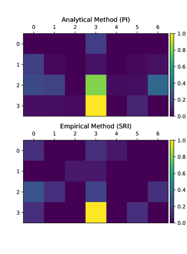
Figure 4: This plot contains the feature impacts (normalized between $0$ and $1$) for the PI, and SRI concerning the total expected reward (sample size $N=300$) approaches with $\epsilon=1$ of the policy $\pi_{A}$ in the Freeway environment (street pixels without the sidewalks).

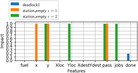
Figure 5: Taxi environment. This diagram plots different advanced property impacts of different PIAs. The original property values (without an attack) are all zero.

Can the PI method generate different property impacts for different advanced property queries? We now show that PI is suited to measure the property impact for properties that can not be expressed by rewards which we call here advanced property queries (see Figure 5).

To make the interpretation of advanced properties more straightforward, we focus on the Taxi environment instead of the Freeway environment and use the advanced property queries deadlock1 and station_empty. Advanced property queries contain, for example, the U-operator (Definition 3.3), which allows the adversary to make sure that certain events happen before other events.

Figure 5 shows the property impact of each attack on the policy and different $\epsilon$-bounded attacks. By attacking the done feature via an PIA (with $\epsilon=1$), it is possible to drive the taxi around without running out of fuel and not finishing jobs while having a passenger on board (deadlock1). Figure 5 also shows that it is possible to let the taxi drive first to the gas station and let it run out of fuel afterwards (station_empty). We observe that for different $\epsilon$-bounds, PIAs have different impacts via features on the temporal logic properties (see station_empty in Figure 5).

Setup					Robustness Checker					PIA			Baseline (FGSM)
Env.	Features	$\epsilon$	Property Query		$P^{max}$	$P$	Impact*	Time		$Impact$	Time		$Impact$	Time
Taxi	done	1	deadlock1		0.44	0.0	0.44	9		0.19	20		0.00	6
	done	1	deadlock2		0.00	0.0	0.00	9		0.00	20		0.00	6
	fuel	2	pass_empty		1.00	0.0	1.00	25		0.25	20		0.00	6
	y	2	$\overline{\textrm{pass}}$_empty		1.00	0.0	1.00	27		1.00	20		1.00	6
	x	1	station_empty		1.00	0.0	1.00	24		1.00	6		1.00	6
	x	1	$\overline{\textrm{station}}$_empty		1.00	0.0	1.00	30		1.00	6		1.00	6
C	obs1_x	1	collision		0.87	0.1	0.86	65		0.46	213		0.87	211
SG	non_renewable	1	blackout		0.97	0.2	0.95	2		0.39	2		0.98	2
SM	sell_price	1	bankruptcy		0.81	0.0	0.81	15		0.08	20		0.00	4

Table 2: Impact* stands for the optimal adversarial attack impact ($|P^{max}-P|$) via the feature specified in Features, $P^{max}$ for the maximal probability $P^{max}(\phi)$ with an attack, $P$ for the original probability $P(\phi)$ (without an attack), Time in seconds, C for Collision Avoidance, SG for Smart Grid, SM for Stock Market, Baseline is a standard FGSM attack on the whole observation. We observe that PIAs perform similarly to FGSM attacks for advanced properties. Our robustness checker shows that our generated PIAs are not necessarily optimal but that they can still modify the targeted property. All our attacks are $\epsilon$-bounded for a fair comparison.

What are the limitations of PIAs? We now analyze the limitations of PIAs and compare them with the FGSM attack (baseline) and the robustness checker. For each experiment, we $\epsilon$-bounded all the generated attacks for a fair comparison. We mainly focus on selected properties from the taxi environment but also include other environments (see Table 2).

Table 2 shows that PIAs, in comparison to FGSM attacks, have similar impacts on temporal logic properties (compare impact columns of PIA and FGSM). For temporal logic properties where some correct decision-making is still needed, PIAs perform better than the FGSM attack (for instance, pass_empty). However, PIAs do not necessarily create a maximal impact on the property values like the robustness checker method (compare PIA impact with Impact*).

After observing the results of the three methods (PIA, FGSM, robustness checker), we can summarize. By verifying the robustness of the trained RL policies, the adversary can already extract for each state the optimal adversarial attack that is part of the most impactful attack. Since PIAs build induced DTMCs and the robustness checker induced MDPs, PIAs are suited for MDPs with more states and transitions before running out of memory (see Gross et al.,, 2022, for more details about the limitations of model checking RL policies) .

Does adversarial training make trained RL policies more robust against PIAs? Figure 5 shows that an adversarial attack (bounded by $\epsilon=1$) on feature $done$ can bring the taxi agent into a deadlock and lets it drive around after the first job is done ($deadlock1=0.19$). To protect the RL agent from this attack, we trained the RL taxi policy over 5000 additional episodes via adversarial training by using our method PIA on the done feature to make the policy more robust against this deadlock attack. The adversarial training improves the feature robustness for the done feature ($0$) but deteriorates the robustness for the other features (all other feature PI-values: $1$). That agrees with the observation that adversarially trained RL policies may be less robust to other types of adversarial attacks (Zhang et al.,, 2020; Korkmaz, 2021a, ; Korkmaz,, 2022). To summarize, adversarial training can improve the RL policy robustness against specific PIAs but may also deteriorate the robustness against other PIAs.

6 CONCLUSION

We presented an analytical method to measure the adversarial attack impact on RL policy properties. This knowledge can be used to craft fine-grained property impact attacks (PIAs) to modify specific values of temporal RL policy properties. Our model checking method allows us to verify if a trained policy is robust against $\epsilon$-bounded PIAs. A learner can use adversarial training in combination with the PIA to obtain more robust policies against specific PIAs.

For future work, it would make sense to combine the current research with countermeasures (Lin et al., 2017b, ; Xiang et al.,, 2018; Havens et al.,, 2018). Furthermore, it would be interesting to analyze adversarial multi-agent reinforcement learning (Figura et al.,, 2021; Zeng et al.,, 2022) in combination with model checking. Interpretable Reinforcement Learning (Davoodi and Komeili,, 2021) can further use the impact results to interpret trained RL policies.

Policy	Env.	Layers	Neurons	LR	Batch	Episodes	Reward
$\pi_{A}$	Freeway	4	512	0.0001	100	10000	0.96
$\pi_{B}$	Taxi	4	512	0.0001	100	60000	-1220.49
$\pi_{C}$	Collision Avoidance	4	512	0.0001	100	5000	9817.00
$\pi_{D}$	Smart Grid	4	512	0.0001	100	5000	-1000.10
$\pi_{E}$	Stock Market	4	512	0.0001	100	10000	326.00

Table 3: $Reward$ specifies the best reward sliding window over $100$ episodes while training, $LR$ for learning rate, $Batch$ for batch size.

Appendix A Additional Environments

Collision avoidance. This is an environment that contains one agent and two moving obstacles in a two-dimensional grid world. The environment terminates as soon as a collision between the agent and obstacle 1 happens. The environment contains a slickness parameter, which defines the probability that the agent stays in the same cell.

$$S=\{(x,y,obs1\_x,obs1\_y,obs2\_x,obs2\_y,done),...\}$$

$$Act=\{north,east,south,west\}$$

$$rew=\begin{cases}0\text{, if collision with obstacle 1}\\ 100\text{, otherwise}\end{cases}$$

Smart grid. In this environment, a controller controls renewable and non-renewable energy production distribution. The objective is to minimize non-renewable energy production by using renewable technologies. If the energy consumption exceeds production, it leads to a blackout. Furthermore, if there is too much energy in the electricity network, the energy production shuts down.

$$S=\{(energy,blackout,renewable,$$

$$non\_renewable,consumption),...\}$$

$$Act=\{increase\_non\_renewable,$$

$$increase\_non\_renewable,$$

$$decrease\_renewable,decrease\_both\}$$

$$rew=\begin{cases}-max(no\_renewable-renewable,0),\\ \text{if no blackout.}\\ -1000\text{, otherwise}\end{cases}$$

Stock market. This environment is a simplified version of a stock market simulation. The agent starts with an initial capital and has to increase it through buying and selling stocks without running into bankruptcy.

$$S=\{(buy\_price,sell\_price,capital,stocks,$$

$$last\_action\_price),...\}$$

$$Act=\{buy,hold,sell\}$$

$$rew=\begin{cases}\text{max(capital - initial capital, 0), if hold.}\\ max(floor(\frac{capital}{buy\_price}),0)\text{, if buy.}\\ max(capital+\text{number of stocks}\\ \text{times sell\_price - initial capital, 0), if sell.}\\ \end{cases}$$

Appendix B Deep RL Training

The training parameters of our trained policies can be found in Table 3. For all training runs we set the seed of numpy, PyTorch and Storm to 128. All RL policies were trained with the standard deep Q-learning algorithm (Mnih et al.,, 2013). With $\epsilon=1$, $\epsilon_{decay}=0.99999$ ($\epsilon_{decay}=0.9999$ for freeway and Collision Avoidance), $\epsilon_{min}=0.1$, $\gamma=0.99$, and a target network replacement of 100.

Appendix C New COOL-MC Extensions

COOL-MC (Gross et al.,, 2022) provides a framework for connecting state-of-the-art (deep) reinforcement learning (RL) with modern model checking. In particular, COOL-MC extends the OpenAI Gym to support RL training on PRISM environments and allows verification of the trained RL policies via the Storm model checker (Hensel et al.,, 2022). COOL-MC is available on GitHub (https://github.com/LAVA-LAB/COOL-MC).

We extended COOL-MC with an adversarial RL that allows the impact measurement of adversarial attacks on RL policy properties. Furthermore, we extended COOL-MC to support our proposed robustness checker. Both extensions can be found in the branch mc_pia in the GitHub Repository (https://github.com/LAVA-LAB/MC˙PIA).

REFERENCES

- Amodei et al., (2016) Amodei, D., Olah, C., Steinhardt, J., Christiano, P. F., Schulman, J., and Mané, D. (2016). Concrete problems in AI safety. CoRR, abs/1606.06565.
- Baier and Katoen, (2008) Baier, C. and Katoen, J. (2008). Principles of model checking. MIT Press.
- Boron and Darken, (2020) Boron, J. and Darken, C. (2020). Developing combat behavior through reinforcement learning in wargames and simulations. In 2020 IEEE Conference on Games (CoG), pages 728–731. IEEE.
- Bouton et al., (2019) Bouton, M., Karlsson, J., Nakhaei, A., Fujimura, K., Kochenderfer, M. J., and Tumova, J. (2019). Reinforcement learning with probabilistic guarantees for autonomous driving. CoRR, abs/1904.07189.
- Carlini and Wagner, (2017) Carlini, N. and Wagner, D. A. (2017). Towards evaluating the robustness of neural networks. In IEEE Symposium on Security and Privacy, pages 39–57. IEEE Computer Society.
- Cassez et al., (2005) Cassez, F., David, A., Fleury, E., Larsen, K. G., and Lime, D. (2005). Efficient on-the-fly algorithms for the analysis of timed games. In CONCUR, volume 3653 of Lecture Notes in Computer Science, pages 66–80. Springer.
- Chan et al., (2020) Chan, P. P. K., Wang, Y., and Yeung, D. S. (2020). Adversarial attack against deep reinforcement learning with static reward impact map. In AsiaCCS, pages 334–343. ACM.
- Chatterjee et al., (2017) Chatterjee, K., Novotný, P., Pérez, G. A., Raskin, J., and Zikelic, D. (2017). Optimizing expectation with guarantees in pomdps. In AAAI, pages 3725–3732. AAAI Press.
- Chen et al., (2019) Chen, T., Liu, J., Xiang, Y., Niu, W., Tong, E., and Han, Z. (2019). Adversarial attack and defense in reinforcement learning-from AI security view. Cybersecur., 2(1):11.
- Clark et al., (2018) Clark, G. W., Doran, M. V., and Glisson, W. (2018). A malicious attack on the machine learning policy of a robotic system. In TrustCom/BigDataSE, pages 516–521. IEEE.
- Courcoubetis and Yannakakis, (1988) Courcoubetis, C. and Yannakakis, M. (1988). Verifying temporal properties of finite-state probabilistic programs. In FOCS, pages 338–345. IEEE Computer Society.
- Courcoubetis and Yannakakis, (1995) Courcoubetis, C. and Yannakakis, M. (1995). The complexity of probabilistic verification. J. ACM, 42(4):857–907.
- David et al., (2015) David, A., Jensen, P. G., Larsen, K. G., Mikucionis, M., and Taankvist, J. H. (2015). Uppaal stratego. In TACAS, volume 9035 of Lecture Notes in Computer Science, pages 206–211. Springer.
- Davoodi and Komeili, (2021) Davoodi, O. and Komeili, M. (2021). Feature-based interpretable reinforcement learning based on state-transition models. In SMC, pages 301–308. IEEE.
- Dräger et al., (2015) Dräger, K., Forejt, V., Kwiatkowska, M. Z., Parker, D., and Ujma, M. (2015). Permissive controller synthesis for probabilistic systems. Log. Methods Comput. Sci., 11(2).
- Farazi et al., (2021) Farazi, N. P., Zou, B., Ahamed, T., and Barua, L. (2021). Deep reinforcement learning in transportation research: A review. Transportation Research Interdisciplinary Perspectives, 11:100425.
- Figura et al., (2021) Figura, M., Kosaraju, K. C., and Gupta, V. (2021). Adversarial attacks in consensus-based multi-agent reinforcement learning. In ACC, pages 3050–3055. IEEE.
- Fulton and Platzer, (2019) Fulton, N. and Platzer, A. (2019). Verifiably safe off-model reinforcement learning. In TACAS (1), volume 11427 of Lecture Notes in Computer Science, pages 413–430. Springer.
- Gehr et al., (2018) Gehr, T., Mirman, M., Drachsler-Cohen, D., Tsankov, P., Chaudhuri, S., and Vechev, M. T. (2018). AI2: safety and robustness certification of neural networks with abstract interpretation. In IEEE Symposium on Security and Privacy, pages 3–18. IEEE Computer Society.
- Gleave et al., (2020) Gleave, A., Dennis, M., Wild, C., Kant, N., Levine, S., and Russell, S. (2020). Adversarial policies: Attacking deep reinforcement learning. In ICLR. OpenReview.net.
- Goodfellow et al., (2015) Goodfellow, I. J., Shlens, J., and Szegedy, C. (2015). Explaining and harnessing adversarial examples. In ICLR.
- Gross et al., (2022) Gross, D., Jansen, N., Junges, S., and Pérez, G. A. (2022). Cool-mc: A comprehensive tool for reinforcement learning and model checking. In SETTA. Springer.
- Hahn et al., (2019) Hahn, E. M., Perez, M., Schewe, S., Somenzi, F., Trivedi, A., and Wojtczak, D. (2019). Omega-regular objectives in model-free reinforcement learning. In TACAS (1), volume 11427 of LNCS, pages 395–412. Springer.
- Hansson and Jonsson, (1994) Hansson, H. and Jonsson, B. (1994). A logic for reasoning about time and reliability. Formal Aspects Comput., 6(5):512–535.
- Hasanbeig et al., (2019) Hasanbeig, M., Kroening, D., and Abate, A. (2019). Towards verifiable and safe model-free reinforcement learning. In OVERLAY@AI*IA, volume 2509 of CEUR Workshop Proceedings, page 1. CEUR-WS.org.
- Hasanbeig et al., (2020) Hasanbeig, M., Kroening, D., and Abate, A. (2020). Deep reinforcement learning with temporal logics. In FORMATS, volume 12288 of LNCS, pages 1–22. Springer.
- Havens et al., (2018) Havens, A. J., Jiang, Z., and Sarkar, S. (2018). Online robust policy learning in the presence of unknown adversaries. In NeurIPS, pages 9938–9948.
- Hensel et al., (2022) Hensel, C., Junges, S., Katoen, J., Quatmann, T., and Volk, M. (2022). The probabilistic model checker storm. Int. J. Softw. Tools Technol. Transf., 24(4):589–610.
- (29) Huang, S. H., Papernot, N., Goodfellow, I. J., Duan, Y., and Abbeel, P. (2017a). Adversarial attacks on neural network policies. In ICLR. OpenReview.net.
- (30) Huang, X., Kwiatkowska, M., Wang, S., and Wu, M. (2017b). Safety verification of deep neural networks. In CAV (1), volume 10426 of Lecture Notes in Computer Science, pages 3–29. Springer.
- Ilahi et al., (2022) Ilahi, I., Usama, M., Qadir, J., Janjua, M. U., Al-Fuqaha, A. I., Hoang, D. T., and Niyato, D. (2022). Challenges and countermeasures for adversarial attacks on deep reinforcement learning. IEEE Trans. Artif. Intell., 3(2):90–109.
- Katz et al., (2017) Katz, G., Barrett, C. W., Dill, D. L., Julian, K., and Kochenderfer, M. J. (2017). Reluplex: An efficient SMT solver for verifying deep neural networks. In CAV (1), volume 10426 of Lecture Notes in Computer Science, pages 97–117. Springer.
- Katz et al., (2019) Katz, G., Huang, D. A., Ibeling, D., Julian, K., Lazarus, C., Lim, R., Shah, P., Thakoor, S., Wu, H., Zeljic, A., Dill, D. L., Kochenderfer, M. J., and Barrett, C. W. (2019). The marabou framework for verification and analysis of deep neural networks. In CAV (1), volume 11561 of Lecture Notes in Computer Science, pages 443–452. Springer.
- (34) Korkmaz, E. (2021a). Adversarial training blocks generalization in neural policies. In NeurIPS 2021 Workshop on Distribution Shifts: Connecting Methods and Applications.
- (35) Korkmaz, E. (2021b). Investigating vulnerabilities of deep neural policies. In UAI, volume 161 of Proceedings of Machine Learning Research, pages 1661–1670. AUAI Press.
- Korkmaz, (2022) Korkmaz, E. (2022). Deep reinforcement learning policies learn shared adversarial features across mdps. In AAAI, pages 7229–7238. AAAI Press.
- Kwiatkowska et al., (2011) Kwiatkowska, M. Z., Norman, G., and Parker, D. (2011). PRISM 4.0: Verification of probabilistic real-time systems. In CAV, volume 6806 of Lecture Notes in Computer Science, pages 585–591. Springer.
- Lee et al., (2021) Lee, X. Y., Esfandiari, Y., Tan, K. L., and Sarkar, S. (2021). Query-based targeted action-space adversarial policies on deep reinforcement learning agents. In ICCPS, pages 87–97. ACM.
- Lee et al., (2020) Lee, X. Y., Ghadai, S., Tan, K. L., Hegde, C., and Sarkar, S. (2020). Spatiotemporally constrained action space attacks on deep reinforcement learning agents. In AAAI, pages 4577–4584. AAAI Press.
- Levine et al., (2016) Levine, S., Finn, C., Darrell, T., and Abbeel, P. (2016). End-to-end training of deep visuomotor policies. J. Mach. Learn. Res., 17:39:1–39:40.
- (41) Lin, Y., Hong, Z., Liao, Y., Shih, M., Liu, M., and Sun, M. (2017a). Tactics of adversarial attack on deep reinforcement learning agents. In ICLR (Workshop). OpenReview.net.
- (42) Lin, Y., Liu, M., Sun, M., and Huang, J. (2017b). Detecting adversarial attacks on neural network policies with visual foresight. CoRR, abs/1710.00814.
- Littman et al., (2017) Littman, M. L., Topcu, U., Fu, J., Isbell, C., Wen, M., and MacGlashan, J. (2017). Environment-independent task specifications via GLTL. arXiv preprint 1704.04341.
- Liu et al., (2022) Liu, Z., Guo, Z., Cen, Z., Zhang, H., Tan, J., Li, B., and Zhao, D. (2022). On the robustness of safe reinforcement learning under observational perturbations. CoRR, abs/2205.14691.
- Mnih et al., (2013) Mnih, V., Kavukcuoglu, K., Silver, D., Graves, A., Antonoglou, I., Wierstra, D., and Riedmiller, M. A. (2013). Playing atari with deep reinforcement learning. CoRR, abs/1312.5602.
- Mnih et al., (2015) Mnih, V., Kavukcuoglu, K., Silver, D., Rusu, A. A., Veness, J., Bellemare, M. G., Graves, A., Riedmiller, M. A., Fidjeland, A., Ostrovski, G., Petersen, S., Beattie, C., Sadik, A., Antonoglou, I., King, H., Kumaran, D., Wierstra, D., Legg, S., and Hassabis, D. (2015). Human-level control through deep reinforcement learning. Nat., 518(7540):529–533.
- Moos et al., (2022) Moos, J., Hansel, K., Abdulsamad, H., Stark, S., Clever, D., and Peters, J. (2022). Robust reinforcement learning: A review of foundations and recent advances. Machine Learning and Knowledge Extraction, 4(1):276–315.
- Nakabi and Toivanen, (2021) Nakabi, T. A. and Toivanen, P. (2021). Deep reinforcement learning for energy management in a microgrid with flexible demand. Sustainable Energy, Grids and Networks, 25:100413.
- Pinto et al., (2017) Pinto, L., Davidson, J., Sukthankar, R., and Gupta, A. (2017). Robust adversarial reinforcement learning. In ICML, volume 70 of Proceedings of Machine Learning Research, pages 2817–2826. PMLR.
- Rakhsha et al., (2020) Rakhsha, A., Radanovic, G., Devidze, R., Zhu, X., and Singla, A. (2020). Policy teaching via environment poisoning: Training-time adversarial attacks against reinforcement learning. In ICML, volume 119 of Proceedings of Machine Learning Research, pages 7974–7984. PMLR.
- Ruan et al., (2018) Ruan, W., Huang, X., and Kwiatkowska, M. (2018). Reachability analysis of deep neural networks with provable guarantees. In IJCAI, pages 2651–2659. ijcai.org.
- Sadigh et al., (2014) Sadigh, D., Kim, E. S., Coogan, S., Sastry, S. S., and Seshia, S. A. (2014). A learning based approach to control synthesis of markov decision processes for linear temporal logic specifications. In CDC, pages 1091–1096. IEEE.
- Sutton and Barto, (2018) Sutton, R. S. and Barto, A. G. (2018). Reinforcement learning: An introduction. MIT press.
- Vamplew et al., (2022) Vamplew, P., Smith, B. J., Källström, J., de Oliveira Ramos, G., Radulescu, R., Roijers, D. M., Hayes, C. F., Heintz, F., Mannion, P., Libin, P. J. K., Dazeley, R., and Foale, C. (2022). Scalar reward is not enough: a response to silver, singh, precup and sutton (2021). Auton. Agents Multi Agent Syst., 36(2):41.
- Wang et al., (2020) Wang, Y., Roohi, N., West, M., Viswanathan, M., and Dullerud, G. E. (2020). Statistically model checking PCTL specifications on markov decision processes via reinforcement learning. In CDC, pages 1392–1397. IEEE.
- Xiang et al., (2018) Xiang, Y., Niu, W., Liu, J., Chen, T., and Han, Z. (2018). A pca-based model to predict adversarial examples on q-learning of path finding. In DSC, pages 773–780. IEEE.
- Yu and Sun, (2022) Yu, M. and Sun, S. (2022). Natural black-box adversarial examples against deep reinforcement learning. In AAAI, pages 8936–8944. AAAI Press.
- Zeng et al., (2022) Zeng, L., Qiu, D., and Sun, M. (2022). Resilience enhancement of multi-agent reinforcement learning-based demand response against adversarial attacks. Applied Energy, 324:119688.
- Zhang et al., (2020) Zhang, H., Chen, H., Xiao, C., Li, B., Liu, M., Boning, D. S., and Hsieh, C. (2020). Robust deep reinforcement learning against adversarial perturbations on state observations. In NeurIPS.