Protocol selection for second-order consensus against disturbance

Abstract

Noticing that both the absolute and relative velocity protocols can solve the second-order consensus of multi-agent systems, this paper aims to investigate which of the above two protocols has better anti-disturbance capability, in which the anti-disturbance capability is measured by the ${\mathcal{L}}_{2}\$gain from the disturbance to the consensus error. More specifically, by the orthogonal transformation technique, the analytic expression of the ${\mathcal{L}}_{2}\$gain of the second-order multi-agent system with absolute velocity protocol is firstly derived, followed by the counterpart with relative velocity protocol. It is shown that both the ${\mathcal{L}}_{2}\$gains for absolute and relative velocity protocols are determined only by the minimum non-zero eigenvalue of Laplacian matrix and the tunable gains of the state and velocity. Then, we establish the graph conditions to tell which protocol has better anti-disturbance capability. Moreover, we propose a two-step scheme to improve the anti-disturbance capability of second-order multi-agent systems. Finally, simulations are given to illustrate the effectiveness of our findings.

[1] organization=Shaanxi Key Laboratory of Space Solar Power Station System, School of Mechano-electronic Engineering, Xidian University, city=Xi’an, postcode=710071, country=China [2] organization=School of Astronautics, Northwestern Polytechnical University, city=Xi’an, postcode=710072, country=China

1 Introduction

Over the past decades, the distributed coordination of multi-agent systems (MASs) has been extensively investigated in control community. As a fundamental issue in multi-agent coordination, consensus problem has attracted tremendous attention. Roughly speaking, consensus means that a group of agents reaches an agreement regarding a common quantity of interest by designing appropriate communication protocol [1].

In retrospect, for the consensus problem, agents are assumed to took first-order dynamics in early seminal works [2, 3, 4]. However, the first-order dynamics model is hardly capable of describing many mechanical systems. Therefore, numerous researchers started to investigate the consensus protocols for second-order MASs to overcome this shortcoming. Subsequently, two classic second-order consensus protocols emerged which employed different treatments to velocity information. One protocol proposed in [5] introduced the absolute velocity information of the agent itself as the local feedback. Another protocol devised in [6] required each agent to use the relative velocity measurements with respect to its neighbors. Then a series of researches on second-order consensus sprang up. More general forms of second-order consensus protocols were studied in [7, 8, 9]. Some results took the communication delay into consideration [10, 11, 12]. The authors in [13] addressed the consensus of second-order MASs with limited agent interaction ranges. In order to reduce the resource consumption, the event-based consensus protocol was developed for second-order MASs in [14]. The resilient consensus was studied in [15] for second-order MASs with faulty or malicious agents. The authors in [16, 17, 18, 19] investigated the consensus of heterogeneous and hybrid MASs, in which agents have different dynamics behaviours.

Since the disturbance is rife in reality, it is of great significance to investigate the anti-disturbance capability for second-order MASs with absolute or relative velocity protocol. In literature, the ${\mathcal{L}}_{2}\$gain is popular in MAS community to characterize the influence of disturbance on the consensus. For example, by LMIs technique, the ${\mathcal{L}}_{2}\$gain optimal consensus is considered in [20, 21, 22, 23, 24, 25, 26, 27]. In a separate direction, some studies tapped into the role of networks on the ${\mathcal{L}}_{2}\$gain of MASs [28, 29, 30, 31]. In [28], the authors built the relation between the ${\mathcal{L}}_{2}\$gain of first-order MASs and the minimum non-zero eigenvalue of the Laplacian matrix associated with the undirected graph. As pointed out in [29], the ${\mathcal{L}}_{2}\$gain of first-order leader-follower MASs on undirected graphs relies on the minimum eigenvalue of the grounded Laplacian matrix. For first-order leader-follower MASs on directed graphs, it was shown in [30] that the ${\mathcal{L}}_{2}\$gain of first-order leader-follower MASs on directed graphs depends on the minimum singular value of the grounded Laplacian matrix. Besides, the authors in [31] analyzed the ${\mathcal{L}}_{2}\$gain of second-order leader-follower MASs with the relative velocity protocol in the presence of communication errors and measurement errors, and derived the analytic expressions of ${\mathcal{L}}_{2}\$gain for a class of special directed networks in which the in-degree of each node was assumed to be the same. Note that the second-order consensus protocols in all aforementioned literature were founded on the basic structures of two classic absolute velocity protocol [5] and relative velocity protocol [6]. Therefore, it is of great significance to study the analytic expressions of ${\mathcal{L}}_{2}\$gains for the second-order MASs with general absolute and relative velocity protocols and develop the graph conditions to tell which one of the above two protocols has better anti-disturbance capability for the second-order consensus. As far as we known, no previous study has investigated these issues.

Motivated by the above observations, this paper aims to investigate which one of the absolute and relative velocity protocols has better anti-disturbance capability for consensus of second-order MASs. The considered problem is challenging as the general communication topology results in difficulty to establish the quantitative relations between weighted adjacency matrix, tunable gains and the anti-disturbance capability. In this paper, the anti-disturbance capability is measured by the ${\mathcal{L}}_{2}\$gain from the disturbance to the consensus error, and we intend to establish the quantitative relations between weighted adjacency matrix, tunable gains and anti-disturbance capability for the second-order MASs with absolute and relative velocity protocols, respectively. Furthermore, on the basis of the established quantitative relations, we give the graph conditions of protocol selection for better anti-disturbance capability. Our contributions are summarized as follows:

• By the orthogonal transformation technique, we establish the quantitative relations between weighted adjacency matrix, tunable gains and the ${\mathcal{L}}_{2}\$gains for the second-order MASs with absolute and relative velocity protocols, respectively. It is shown that the ${\mathcal{L}}_{2}\$gains are inversely proportional to both the minimum non-zero eigenvalue of the Laplacian matrix and the tunable gains.

• The protocol selection criteria are developed for the second-order MASs. We give the graph conditions to tell which one of the absolute and relative velocity protocols has better anti-disturbance capability.

• For any given connected undirected graph, we present a two-step scheme to improve the anti-disturbance capability of second-order MASs. It is tractable and highly effecient when the network is unable to rearrange or expand.

The rest of this paper is organized as follows. In Section 2, we give some preliminaries and state the problem. The quantitative relations between weighted adjacency matrix, tunable gains and the ${\mathcal{L}}_{2}\$gains, and the graph conditions for better anti-disturbance capability are given in Section 3. In Section 4, simulations are given to illustrate the effectiveness of theoretical results. We conclude our work in Section 5.

Notations: Throughout this paper, $\mathbb{N}$ indicates the set of nonnegative integers, $\mathbb{R}$ denotes the set of real numbers, $\mathbb{R}^{+}$ is the set of positive real numbers, $\mathbb{R}^{n}$ is the $n$-dimensional real column vector space, $\mathbb{R}^{m\times n}$ represents the $m\times n$ real matrix space. Denote the all-one and all-zero matrices with appropriate dimensions by $\mathbf{1}$ and $\mathbf{0}$, respectively. Specifically, $\mathbf{1}_{n}$ and $\mathbf{0}_{n}$ refer to the $n\times 1$ all ones and all zeros column vectors, respectively. Let $I_{n}$ be the $n$-dimensional identity matrix. $\mathbf{j}$ stands for the imaginary unit. For a matrix $X$, $X^{\top}$ labels its transpose, $X^{H}$ denotes its conjugate transpose, and $\sigma_{max}(X)$ represents its maximum singular value. For a Hermitian matrix $X$, $\lambda_{max}(X)$ denotes its maximum eigenvalue. $X\in\mathbb{R}^{n\times n}$ is orthogonal if $X^{\top}X=XX^{\top}=I_{n}$. $\text{diag}\{a_{1},a_{2},\dots,a_{n}\}$ designates a diagonal matrix, where $a_{i}$ is the $i_{\text{th}}$ diagonal element. Define a set $\mathcal{I}_{n}=\{1,2,\dots,n\}$. Null set is represented by $\emptyset$. For the given set $\mathcal{R}_{1}$ and $\mathcal{R}_{2}$, $\mathcal{R}_{1}\cup\mathcal{R}_{2}$ and $\mathcal{R}_{1}\cap\mathcal{R}_{2}$ indicate the set union and set intersection, respectively. $\mathcal{L}_{2}\left[0,\infty\right)$ dictates the space of square-integrable vector functions, i.e., $f(t)\in\mathcal{L}_{2}\left[0,\infty\right)$ if and only if $\int_{0}^{\infty}f^{\top}(t)f(t)\,\mathrm{d}t<\infty$.

2 Preliminaries and problem statement

2.1 Preliminaries

Let $\mathcal{G}=(\mathcal{V},\mathcal{E},\mathcal{A})$ be a weighted undirected graph with $n$ vertices, where $\mathcal{V}=\{s_{1},s_{2},\dots,s_{n}\}$ is the set of vertices, $\mathcal{E}\subseteq\mathcal{V}\times\mathcal{V}$ is the set of edges, and $\mathcal{A}=[a_{ij}]_{n\times n}$ is the weighted adjacency matrix with $a_{ij}=a_{ji}\geq 0$. $\varepsilon_{ij}=(s_{i},s_{j})\in\mathcal{E}$ if and only if there exist information exchanges between vertices $s_{i}$ and $s_{j}$. The adjacency element associated with the edge $\varepsilon_{ij}$ is $a_{ij}$, and $a_{ij}>0$ if and only if $\varepsilon_{ij}\in\mathcal{E}$. Moreover, suppose that $\mathcal{G}$ has no self-cycles for every node, i.e., $a_{ii}=0$. A path between two distinct vertices $v_{i}$ and $v_{j}$ is a finite-ordered sequence of distinct edges in $\mathcal{G}$ with the form $(v_{i},v_{k_{1}}),(v_{k_{1}},v_{k_{2}}),\dots,(v_{k_{l}},v_{j})$. An undirected graph is called connected if there exists a path between any two distinct vertices of the graph. The Laplacian matrix $L=[l_{ij}]\in\mathbb{R}^{n\times n}$ associated with graph $\mathcal{G}$ is defined as $l_{ii}=\sum_{j=1,j\neq i}^{n}a_{ij}$ and $l_{ij}=-a_{ij}$, $j\neq i$.

The following definitions and lemmas will be utilized to establish the main results.

Definition 1 ([32]).

For an undirected graph $\mathcal{G}$ with $n$ vertices, the network density $d$ is defined as

$$d=\frac{\epsilon}{\dfrac{1}{2}n(n-1)},$$

where $\epsilon$ represents the total number of undirected edges in the graph $\mathcal{G}$ and $\frac{1}{2}n(n-1)$ is the maximum theoretical number of undirected edges between the $n$ vertices.

Lemma 1 ([2]).

For the Laplacian matrix $L$ associated with the undirected graph $\mathcal{G}$, $L$ possesses a simple zero eigenvalue associated with eigenvector $\mathbf{1}_{n}$ if and only if $\mathcal{G}$ is connected. In addition, all the other non-zero eigenvalues are positive.

Denote the eigenvalues of Laplacian matrix $L$ associated with graph $\mathcal{G}$ by $\lambda_{i}$, $i\in\mathcal{I}_{n}$. For convenience, if $\mathcal{G}$ is undirected and connected, suppose that $0=\lambda_{1}<\lambda_{2}\leq\cdots\leq\lambda_{n}$ and let $\Gamma=\{\lambda_{2},\dots,\lambda_{n}\}$ be the set of all non-zero eigenvalues of $L$.

Lemma 2 ([26]).

Let $\mathcal{G}$ be a connected undirected graph with a Laplacian matrix $L\in\mathbb{R}^{n\times n}$ and $\Phi_{n}=[\varphi_{ij}]\in\mathbb{R}^{n\times n}$ be a symmetric matrix whose elements are given as

$$\varphi_{ij}=\begin{dcases}\frac{n-1}{n},&i=j,\\ -\frac{1}{n},&i\neq j.\end{dcases}$$

Then, there exists an orthogonal matrix $Q\in\mathbb{R}^{n\times n}$ with the last column being $\frac{\mathbf{1}_{n}}{\sqrt{n}}$ such that

$$Q^{\top}\Phi_{n}Q=\bar{\Phi}_{n}=\begin{bmatrix}I_{n-1}&\mathbf{0}_{n-1}\\ \mathbf{0}_{n-1}^{\top}&0\end{bmatrix}$$ (1)

and

$$Q^{\top}LQ=\bar{L}=\begin{bmatrix}\bar{L}_{1}&\mathbf{0}_{n-1}\\ \mathbf{0}_{n-1}^{\top}&0\end{bmatrix},$$ (2)

where $\bar{L}_{1}\in\mathbb{R}^{(n-1)\times(n-1)}$ is positive definite.

Definition 2 ([33]).

The $H_{\infty}$ norm of an asymptotically stable continuous-time transfer matrix $T(s)$ is defined as

$$\|T(s)\|_{\infty}=\sup_{\upsilon\in\mathbb{R}}\sigma_{max}\big{[}T(\mathbf{j}\upsilon)\big{]}.$$

2.2 Problem statement

In this paper, we consider a MAS consisting of $n$ agents with double-integrator dynamics

$$\dot{x}_{i}(t) =v_{i}(t),$$ (3)

$$\dot{v}_{i}(t) =u_{i}(t)+\omega_{i}(t),i\in\mathcal{I}_{n},$$

where $x_{i}(t)\in\mathbb{R}$, $v_{i}(t)\in\mathbb{R}$, $u_{i}(t)\in\mathbb{R}$, and $\omega_{i}(t)\in\mathbb{R}$ are the position-like, velocity-like, control input and external disturbance of the $i_{\text{th}}$ agent, respectively. In addition, we suppose that $\omega_{i}(t)\in\mathcal{L}_{2}\left[0,\infty\right)$.

The following definition of second-order consensus given in [8] is useful.

Definition 3 ([8]).

The second-order MAS (3) is said to reach consensus if

$$\begin{gathered}\lim_{t\to\infty}\|x_{i}(t)-x_{j}(t)\|=0,\forall i,j\in\mathcal{I}_{n},\\ \lim_{t\to\infty}\|v_{i}(t)-v_{j}(t)\|=0,\forall i,j\in\mathcal{I}_{n},\end{gathered}$$

for any initial condition.

In the absence of disturbance, i.e., $\omega_{i}(t)=0$, as one can observe from [7] and [8], both the general absolute and relative velocity protocols (4) and (5) can solve the second-order consensus under the condition that $\mathcal{G}$ is a connected undirected graph.

$$u_{i}(t)=\alpha\sum_{j=1}^{n}{a_{ij}\big{[}x_{j}(t)-x_{i}(t)\big{]}}-\beta v_{i}(t),$$ (4)

$$u_{i}(t)=\alpha\sum_{j=1}^{n}{a_{ij}\big{[}x_{j}(t)-x_{i}(t)\big{]}}+\beta\sum_{j=1}^{n}{a_{ij}\big{[}v_{j}(t)-v_{i}(t)\big{]}},$$ (5)

where $a_{ij}$ is the $(i,j)_{\text{th}}$ entry of the weighted adjacency matrix $\mathcal{A}$ associated with undirected graph $\mathcal{G}$, and the positive constant $\alpha$ and $\beta$ are tunable gains.

Different from existing works, we restrict our attention to investigate which one of the above protocols has better anti-disturbance capability. And we aim to bring forward simple graph conditions for protocol selection.

Define

$$y_{i}^{x}(t)=x_{i}(t)-\frac{1}{n}\sum_{j=1}^{n}x_{j}(t),~{}i\in\mathcal{I}_{n},$$ (6)

and

$$y_{i}^{v}(t)=v_{i}(t)-\frac{1}{n}\sum_{j=1}^{n}v_{j}(t),~{}i\in\mathcal{I}_{n},$$ (7)

for each agent to measure the consensus error of position and velocity, respectively. Aggregating the outputs of all agents into a vector $y(t)\in\mathbb{R}^{2n}$ gives rise to

$$y(t)=\begin{bmatrix}y^{x}(t)\\ y^{v}(t)\end{bmatrix},$$ (8)

where the agglomerate vector $y^{x}(t)=\big{[}y_{1}^{x}(t),\dots,y_{n}^{x}(t)\big{]}^{\top}$ and $y^{v}(t)=\big{[}y_{1}^{v}(t),\dots,y_{n}^{v}(t)\big{]}^{\top}$ denote the collective position error and collective velocity error, respectively. Substituting the protocols (4) and (5) into (3), respectively, and taking (8) into consideration yield the closed-loop systems (9) and (10), respectively. Here, the nominal output $y(t)$ is termed as collective consensus error.

$$\begin{dcases}\begin{bmatrix}\dot{x}(t)\\ \dot{v}(t)\end{bmatrix}=\begin{bmatrix}\mathbf{0}&I_{n}\\ -\alpha L&-\beta I_{n}\end{bmatrix}\begin{bmatrix}x(t)\\ v(t)\end{bmatrix}+\begin{bmatrix}\mathbf{0}\\ I_{n}\end{bmatrix}\omega(t),\\ y(t)=\begin{bmatrix}\Phi_{n}&\mathbf{0}\\ \mathbf{0}&\Phi_{n}\end{bmatrix}\begin{bmatrix}x(t)\\ v(t)\end{bmatrix},\end{dcases}$$ (9)

$$\begin{dcases}\begin{bmatrix}\dot{x}(t)\\ \dot{v}(t)\end{bmatrix}=\begin{bmatrix}\mathbf{0}&I_{n}\\ -\alpha L&-\beta L\end{bmatrix}\begin{bmatrix}x(t)\\ v(t)\end{bmatrix}+\begin{bmatrix}\mathbf{0}\\ I_{n}\end{bmatrix}\omega(t),\\ y(t)=\begin{bmatrix}\Phi_{n}&\mathbf{0}\\ \mathbf{0}&\Phi_{n}\end{bmatrix}\begin{bmatrix}x(t)\\ v(t)\end{bmatrix},\end{dcases}$$ (10)

where $x(t)=\big{[}x_{1}(t),\dots,x_{n}(t)\big{]}^{\top}$, $v(t)=\big{[}v_{1}(t),\dots,v_{n}(t)\big{]}^{\top}$, $\omega(t)=\big{[}\omega_{1}(t),\dots,\omega_{n}(t)\big{]}^{\top}$, and $L$ is the Laplacian matrix associated with graph $\mathcal{G}$.

In this paper, we respectively use the $\mathcal{L}_{2}$ gains from the disturbance $\omega(t)$ to collective consensus error $y(t)$ of systems (9) and (10) to measure the anti-disturbance capabilities of the MASs (3)-(4) and (3)-(5). As shown in [34], the $\mathcal{L}_{2}$ gains of systems (9) and (10) are defined by

$$\sup_{\begin{subarray}{c}\omega(t)\neq 0\\ \omega(t)\in\mathcal{L}_{2}\left[0,\infty\right)\end{subarray}}\sqrt{\frac{\int_{0}^{\infty}y^{\top}(t)y(t)\,\mathrm{d}t}{\int_{0}^{\infty}\omega^{\top}(t)\omega(t)\,\mathrm{d}t}}.$$

However, it is difficult to directly use $\mathcal{L}_{2}$ gain to analyze the anti-disturbance capability of the considered MASs. Let $T_{1}(s)$ and $T_{2}(s)$ be the transfer matrices from disturbance $\omega(t)$ to collective consensus error $y(t)$ of the systems (9) and (10), respectively. It follows from [33] that the $\mathcal{L}_{2}$ gains of systems (9) and (10) are equal to $\|T_{1}(s)\|_{\infty}$ and $\|T_{2}(s)\|_{\infty}$, respectively, where $\|T_{i}(s)\|_{\infty}$ refers to the ${H}_{\infty}\$norm of $T_{i}(s)$ $(i=1,2)$. Clearly, smaller ${H}_{\infty}\$norm of transfer matrix means better anti-disturbance capability.

Note that $\|T_{1}(s)\|_{\infty}$ and $\|T_{2}(s)\|_{\infty}$ are easy to tackle. In the following, for connected undirected graph $\mathcal{G}$, we directly use $\|T_{1}(s)\|_{\infty}$ and $\|T_{2}(s)\|_{\infty}$ to characterize the anti-disturbance capabilities of MASs (3)-(4) and (3)-(5), respectively. For convenience, we introduce the following definitions.

Definition 4.

For the second-order MAS (3), assume that $G$ is a connected undirected graph.

• The protocol (4) is said to outperform the protocol (5) if the anti-disturbance capability of MAS (3)-(4) outperforms that of MAS (3)-(5), i.e., $\|T_{1}(s)\|_{\infty}\leq\|T_{2}(s)\|_{\infty}$;

• The protocol (5) is said to outperform the protocol (4) if the anti-disturbance capability of MAS (3)-(5) outperforms that of MAS (3)-(4), i.e., $\|T_{2}(s)\|_{\infty}\leq\|T_{1}(s)\|_{\infty}$;

• The protocol (4) is said to perform as well as the protocol (5) if the MASs (3)-(5) and (3)-(4) have the same anti-disturbance capability, i.e., $\|T_{2}(s)\|_{\infty}\equiv\|T_{1}(s)\|_{\infty}$.

3 Main results

In this section, we will establish the graph conditions to tell which protocol has better anti-disturbance for MAS (3). Prior to stating the main results, we propose a useful lemma.

Lemma 3.

Let $g_{1}(t)=\dfrac{1}{(\alpha t)^{2}}$, $g_{2}(t)=\dfrac{1}{(\alpha t)^{2}-(\sqrt{\Delta}-1)^{2}}$, and $g_{3}(t)=\dfrac{1}{(\alpha t)^{2}-(\sqrt{\Theta}-1)^{2}}$, where $\Delta=(\alpha t+1)^{2}-\beta^{2}$, $\Theta=(\alpha t+1)^{2}-(\beta t)^{2}$, and the constants $\alpha$ and $\beta$ are positive. Then the following statements hold$:$

• $g_{1}(t)$ is decreasing on $(0,+\infty)$;

• $g_{2}(t)$ is decreasing on $(\frac{\beta-1}{\alpha},+\infty)$;

• $g_{3}(t)$ is decreasing on $(0,+\infty)$ if $\beta\leq\alpha$;

• $g_{3}(t)$ is decreasing on $(0,\frac{2\alpha}{\beta^{2}-\alpha^{2}})$ if $\beta>\alpha$.

Proof 1.

Clearly, $g_{1}(t)$ is decreasing with $t$ on $(0,+\infty)$. Let $h_{1}(t)=(\alpha t)^{2}-(\sqrt{\Delta}-1)^{2}$, then it is inferred from $t\in(\frac{\beta-1}{\alpha},+\infty)$ that

$$\frac{\mathrm{d}h_{1}(t)}{\mathrm{d}t} =\frac{2\alpha^{2}t+2\alpha}{\sqrt{(\alpha t+1)^{2}-\beta^{2}}}-2\alpha$$

$$=2\alpha\sqrt{\frac{(\alpha t+1)^{2}}{(\alpha t+1)^{2}-\beta^{2}}}-2\alpha>0.$$

It follows from

$$\frac{\mathrm{d}g_{2}(t)}{\mathrm{d}t}=-\frac{\frac{\mathrm{d}h_{1}(t)}{\mathrm{d}t}}{h_{1}^{2}(t)}<0$$

that $g_{2}(t)$ is a decreasing function of $t$ on $(\frac{\beta-1}{\alpha},+\infty)$.

Likewise, let $h_{2}(t)=(\alpha t)^{2}-(\sqrt{\Theta}-1)^{2}$, then we have

$$\frac{\mathrm{d}h_{2}(t)}{\mathrm{d}t}=\frac{2\alpha(\alpha t+1)-2\beta^{2}t}{\sqrt{(\alpha t+1)^{2}-(\beta t)^{2}}}+2\beta^{2}t-2\alpha.$$

The second derivative of $h_{2}(t)$ turns out to be

$$\frac{\mathrm{d}^{2}h_{2}(t)}{\mathrm{d}t^{2}} =\frac{(2\alpha^{2}-2\beta^{2})\sqrt{\Theta}-\dfrac{2\big{[}\alpha(\alpha t+1)-\beta^{2}t\big{]}^{2}}{\sqrt{\Theta}}}{\Theta}+2\beta^{2}$$

$$=\frac{(2\alpha^{2}-2\beta^{2})\Theta-2\big{[}\alpha(\alpha t+1)-\beta^{2}t\big{]}^{2}}{\Theta^{\frac{3}{2}}}+2\beta^{2}$$

$$=\frac{-2\beta^{2}}{\Theta^{\frac{3}{2}}}+2\beta^{2}.$$

If $\beta\leq\alpha$, we get $\Theta>1,\forall t\in(0,+\infty)$ which means that $\frac{\mathrm{d}^{2}h_{2}(t)}{\mathrm{d}t^{2}}>0,\forall t\in(0,+\infty)$. Combining with the fact $\frac{\mathrm{d}h_{2}(t)}{\mathrm{d}t}\big{|}_{t=0}=0$ gives rise to $\frac{\mathrm{d}h_{2}(t)}{\mathrm{d}t}>0,\forall t\in(0,+\infty)$. Then

$$\frac{\mathrm{d}g_{3}(t)}{\mathrm{d}t}=-\frac{\frac{\mathrm{d}h_{2}(t)}{\mathrm{d}t}}{h_{2}^{2}(t)}<0$$ (11)

holds for any $t\in(0,+\infty)$. Thus, $g_{3}(t)$ is decreasing on $(0,+\infty)$.

Provided that $\beta>\alpha$, we have $\Theta>1,\forall t\in(0,\frac{2\alpha}{\beta^{2}-\alpha^{2}})$ which implies that $\frac{\mathrm{d}^{2}h_{2}(t)}{\mathrm{d}t^{2}}>0,\forall t\in(0,\frac{2\alpha}{\beta^{2}-\alpha^{2}})$. Combining with $\frac{\mathrm{d}h_{2}(t)}{\mathrm{d}t}\big{|}_{t=0}=0$ derives that $\frac{\mathrm{d}h_{2}(t)}{\mathrm{d}t}>0,\forall t\in(0,\frac{2\alpha}{\beta^{2}-\alpha^{2}})$. Then (11) holds for any $t\in(0,\frac{2\alpha}{\beta^{2}-\alpha^{2}})$. Therefore, $g_{3}(t)$ is decreasing on $(0,\frac{2\alpha}{\beta^{2}-\alpha^{2}})$. $\square$

3.1 Anti-disturbance capability of the second-order MAS using absolute velocity information

Theorem 1 gives the analytic expression of the anti-disturbance capability of second-order MAS (3) with absolute velocity protocol (4).

Theorem 1.

Consider MAS (3)-(4) in which $\mathcal{G}$ is a connected undirected graph with Laplacian matrix $L$. Then, we obtain

$$\|T_{1}(s)\|_{\infty}=\begin{dcases}\frac{1}{\sqrt{(\alpha\lambda_{2})^{2}-\Big{[}\sqrt{(\alpha\lambda_{2}+1)^{2}-\beta^{2}}-1\Big{]}^{2}}},&\text{if}~{}~{}0<\beta<\sqrt{(\alpha\lambda_{2})^{2}+2\alpha\lambda_{2}},\\ \frac{1}{\alpha\lambda_{2}},&\text{if}~{}~{}\beta\geq\sqrt{(\alpha\lambda_{2})^{2}+2\alpha\lambda_{2}}.\end{dcases}$$ (12)

Proof 2.

Since the undirected graph $\mathcal{G}$ is connected, it follows from Lemma 2 that there exists an orthogonal matrix $Q\in\mathbb{R}^{n\times n}$ such that (1) and (2) hold. Then introducing the following orthogonal transformation

$$\begin{bmatrix}\hat{x}(t)\\ \hat{v}(t)\end{bmatrix} =\begin{bmatrix}Q^{\top}&\mathbf{0}\\ \mathbf{0}&Q^{\top}\end{bmatrix}\begin{bmatrix}x(t)\\ v(t)\end{bmatrix},$$ (13)

$$\hat{y}(t) =\begin{bmatrix}Q^{\top}&\mathbf{0}\\ \mathbf{0}&Q^{\top}\end{bmatrix}y(t),$$

$$\hat{\omega}(t) =Q^{\top}\omega(t),$$

for system (9) gives rise to

$$\begin{dcases}\begin{bmatrix}\dot{\hat{x}}(t)\\ \dot{\hat{v}}(t)\end{bmatrix}=\begin{bmatrix}\mathbf{0}&I_{n}\\ -\alpha\bar{L}&-\beta I_{n}\end{bmatrix}\begin{bmatrix}\hat{x}(t)\\ \hat{v}(t)\end{bmatrix}+\begin{bmatrix}\mathbf{0}\\ I_{n}\end{bmatrix}\hat{\omega}(t),\\ \hat{y}(t)=\begin{bmatrix}\bar{\Phi}_{n}&\mathbf{0}\\ \mathbf{0}&\bar{\Phi}_{n}\end{bmatrix}\begin{bmatrix}\hat{x}(t)\\ \hat{v}(t)\end{bmatrix},\end{dcases}$$ (14)

where

$$\bar{L}=\begin{bmatrix}\bar{L}_{1}&\mathbf{0}_{n-1}\\ \mathbf{0}_{n-1}^{\top}&0\end{bmatrix}.$$

As evidenced from Lemma 1 and (2), positive definite matrix $\bar{L}_{1}$ possesses the same non-zero eigenvalues of $L$ which implies that $-\bar{L}_{1}$ is Hurwitz stable. Clearly, system (14) is composed of an asymptotically stable subsystem of order $2n-2$ and a marginally stable subsystem of order $2$. Since the asymptotically stable subsystem is observable and the marginally stable subsystem is unobservable, according to [35], $\|T_{1}(s)\|_{\infty}$ is still well-difined and completely determined by the asymptotically stable subsystem. Consider the asymptotically stable subsystem of (14) taking the form of

$$\begin{dcases}\begin{bmatrix}\dot{\hat{x}}^{1}(t)\\ \dot{\hat{v}}^{1}(t)\end{bmatrix}=\begin{bmatrix}\mathbf{0}&I_{n-1}\\ -\alpha\bar{L}_{1}&-\beta I_{n-1}\end{bmatrix}\begin{bmatrix}\hat{x}^{1}(t)\\ \hat{v}^{1}(t)\end{bmatrix}+\begin{bmatrix}\mathbf{0}\\ I_{n-1}\end{bmatrix}\hat{\omega}^{1}(t),\\ \hat{y}^{1}(t)=\begin{bmatrix}I_{n-1}&\mathbf{0}\\ \mathbf{0}&I_{n-1}\end{bmatrix}\begin{bmatrix}\hat{x}^{1}(t)\\ \hat{v}^{1}(t)\end{bmatrix},\end{dcases}$$ (15)

where $\hat{x}^{1}(t)=\begin{bmatrix}I_{n-1}&\mathbf{0}_{n-1}\end{bmatrix}\hat{x}(t)$, $\hat{v}^{1}(t)=\begin{bmatrix}I_{n-1}&\mathbf{0}_{n-1}\end{bmatrix}$   $\hat{v}(t)$ and $\hat{\omega}^{1}(t)=\begin{bmatrix}I_{n-1}&\mathbf{0}_{n-1}\end{bmatrix}\hat{\omega}(t).$ Since $\bar{L}_{1}$ is positive definite, there exists an orthogonal matrix $V\in\mathbb{R}^{(n-1)\times(n-1)}$ such that $V^{\top}\bar{L}_{1}V=\varLambda$, where $\varLambda=\text{diag}\{\lambda_{2},\lambda_{3},\dots,\lambda_{n}\}$ is composed of the non-zero eigenvalues of $L$. Then performing the following orthogonal transformation

$$\begin{bmatrix}\tilde{x}(t)\\ \tilde{v}(t)\end{bmatrix} =\begin{bmatrix}V^{\top}&\mathbf{0}\\ \mathbf{0}&V^{\top}\end{bmatrix}\begin{bmatrix}\hat{x}^{1}(t)\\ \hat{v}^{1}(t)\end{bmatrix},$$ (16)

$$\tilde{y}(t) =\begin{bmatrix}V^{\top}&\mathbf{0}\\ \mathbf{0}&V^{\top}\end{bmatrix}\hat{y}^{1}(t),$$

$$\tilde{\omega}(t) =V^{\top}\hat{\omega}^{1}(t),$$

for the system (15) provides

$$\begin{dcases}\begin{bmatrix}\dot{\tilde{x}}(t)\\ \dot{\tilde{v}}(t)\end{bmatrix}=\begin{bmatrix}\mathbf{0}&I_{n-1}\\ -\alpha\varLambda&-\beta I_{n-1}\end{bmatrix}\begin{bmatrix}\tilde{x}(t)\\ \tilde{v}(t)\end{bmatrix}+\begin{bmatrix}\mathbf{0}\\ I_{n-1}\end{bmatrix}\tilde{\omega}(t),\\ \tilde{y}(t)=\begin{bmatrix}I_{n-1}&\mathbf{0}\\ \mathbf{0}&I_{n-1}\end{bmatrix}\begin{bmatrix}\tilde{x}(t)\\ \tilde{v}(t)\end{bmatrix}.\end{dcases}$$ (17)

Denote the transfer matrix of the system (14), (15) and (17) by $T_{3}(s)$, $T_{4}(s)$ and $T_{5}(s)$, respectively. Through simple calculation, it is easy to verify that

$$\|T_{1}(s)\|_{\infty}=\|T_{3}(s)\|_{\infty}=\|T_{4}(s)\|_{\infty}=\|T_{5}(s)\|_{\infty}.$$ (18)

Then we turn to compute $\|T_{5}(s)\|_{\infty}$.

The transfer matrix $T_{5}(s)$ is shown as

$$T_{5}(s)=\left[\begin{array}[]{ccc}\Xi_{2}&&\\ &\ddots&\\ &&\Xi_{n}\\ \hdashline\Upsilon_{2}&&\\ &\ddots&\\ &&\Upsilon_{n}\end{array}\right],$$

where $\Xi_{i}=\dfrac{1}{s^{2}+\beta s+\alpha\lambda_{i}}$ and $\Upsilon_{i}=\dfrac{s}{s^{2}+\beta s+\alpha\lambda_{i}}$, $i=2,\dots,n$. It can be readily obtained that

$$T_{5}^{H}(\mathbf{j}\upsilon)T_{5}(\mathbf{j}\upsilon)=\begin{bmatrix}\delta_{2}(\upsilon)&&\\ &\ddots&\\ &&\delta_{n}(\upsilon)\end{bmatrix}$$

is diagonal, where

$$\delta_{i}(\upsilon)=\frac{1+\upsilon^{2}}{(\alpha\lambda_{i}-\upsilon^{2})^{2}+(\beta\upsilon)^{2}}>0,~{}i=2,\dots,n,~{}\upsilon\in\mathbb{R}.$$

According to Definition 2 and (18), $\|T_{1}(s)\|_{\infty}$ can be treated as

$$\begin{split}\|T_{1}(s)\|_{\infty}&=\|T_{5}(s)\|_{\infty}\\ &=\sup_{\upsilon\in\mathbb{R}}\sqrt{\lambda_{max}\big{[}T_{5}^{H}(\mathbf{j}\upsilon)T_{5}(\mathbf{j}\upsilon)\big{]}}\\ &=\max_{i=2,\dots,n}\sqrt{\sup_{\upsilon\in\mathbb{R}}\delta_{i}(\upsilon)}.\end{split}$$ (19)

It is inferred from

$$\frac{\mathrm{d}\delta_{i}(\upsilon)}{\mathrm{d}\upsilon}=\frac{-2\upsilon\big{[}\upsilon^{4}+2\upsilon^{2}+\beta^{2}-(\alpha\lambda_{i})^{2}-2\alpha\lambda_{i}\big{]}}{\big{[}\upsilon^{4}+(\beta^{2}-2\alpha\lambda_{i})\upsilon^{2}+(\alpha\lambda_{i})^{2}\big{]}^{2}}=0$$ (20)

that

$$\upsilon\big{[}\upsilon^{4}+2\upsilon^{2}+\beta^{2}-(\alpha\lambda_{i})^{2}-2\alpha\lambda_{i}\big{]}=0.$$ (21)

Obviously, $\sup_{\upsilon\in\mathbb{R}}\delta_{i}(\upsilon)$ depends on $\beta^{2}-(\alpha\lambda_{i})^{2}-2\alpha\lambda_{i}$. If $\beta\geq\sqrt{(\alpha\lambda_{i})^{2}+2\alpha\lambda_{i}}$, by solving (21), it is easy to obtain

$$\sup_{\upsilon\in\mathbb{R}}\delta_{i}(\upsilon)=\delta_{i}(\upsilon^{*}_{i,1})=g_{1}(\lambda_{i})=\frac{1}{(\alpha\lambda_{i})^{2}},$$

where $\upsilon^{*}_{i,1}=0$. If $\beta<\sqrt{(\alpha\lambda_{i})^{2}+2\alpha\lambda_{i}}$, by solving (21), it can be readily concluded that

$$\begin{split}\sup_{\upsilon\in\mathbb{R}}\delta_{i}(\upsilon)=&\delta_{i}(\upsilon^{*}_{i,2})=\delta_{i}(\upsilon^{*}_{i,3})=g_{2}(\lambda_{i})\\ =&\frac{1}{(\alpha\lambda_{i})^{2}-(\sqrt{\Delta_{i}}-1)^{2}}\end{split}$$

where $\upsilon^{*}_{i,2},\upsilon^{*}_{i,3}=\pm\sqrt{\sqrt{\Delta_{i}}-1}$, and $\Delta_{i}=(\alpha\lambda_{i}+1)^{2}-\beta^{2}$. The trajectories of the function $\delta_{i}(\upsilon)$ under the conditions $\beta\geq\sqrt{(\alpha\lambda_{i})^{2}+2\alpha\lambda_{i}}$ and $\beta<\sqrt{(\alpha\lambda_{i})^{2}+2\alpha\lambda_{i}}$ are displayed in Fig. 1.

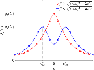
Figure 1: Trajectories of $\delta_{i}(\upsilon)$ under different conditions.

Building on these preliminary observations, we refer to

$$\mathcal{R}_{1}=\Big{\{}r\in\Gamma~{}\big{|}~{}\beta\geq\sqrt{(\alpha r)^{2}+2\alpha r}\Big{\}}$$

and

$$\mathcal{R}_{2}=\Big{\{}r\in\Gamma~{}\big{|}~{}\beta<\sqrt{(\alpha r)^{2}+2\alpha r}\Big{\}}$$

as two sets of non-zero eigenvalues of $L$. Obviously, $\mathcal{R}_{1}\cup\mathcal{R}_{2}=\Gamma$ and $\mathcal{R}_{1}\cap\mathcal{R}_{2}=\emptyset$ hold. We will complete the proof by enumeration.

(I) $\mathcal{R}_{1}=\Gamma$ and $\mathcal{R}_{2}=\emptyset$;

In this case, we have $\beta\geq\sqrt{(\alpha\lambda_{i})^{2}+2\alpha\lambda_{i}},\forall i\in\{2,\dots,n\}$ which leads to $\sup_{\upsilon\in\mathbb{R}}\delta_{i}(\upsilon)=g_{1}{(\lambda_{i})},\forall i\in\{2,\dots,n\}$. Because $0<\lambda_{2}\leq\cdots\leq\lambda_{n}$ and $g_{1}{(t)}$ is decreasing on $(0,+\infty)$, one can deduce that $\max_{i=2,\dots,n}g_{1}{(\lambda_{i})}=g_{1}(\lambda_{2})$. Therefore, (19) can be written as

$$\|T_{1}(s)\|_{\infty}=\max_{i=2,\dots,n}\sqrt{g_{1}{(\lambda_{i})}}=\sqrt{g_{1}(\lambda_{2})}=\frac{1}{\alpha\lambda_{2}}.$$

(II) $\mathcal{R}_{1}=\emptyset$ and $\mathcal{R}_{2}=\Gamma$;

Under this circumstance, we can obtain that $\beta<\sqrt{(\alpha\lambda_{i})^{2}+2\alpha\lambda_{i}},\forall i\in\{2,\dots,n\}$ which leads to

$$\lambda_{i}>\frac{\sqrt{1+\beta^{2}}-1}{\alpha}>\frac{\beta-1}{\alpha},\forall i\in\{2,\dots,n\}$$

and $\sup_{\upsilon\in\mathbb{R}}\delta_{i}(\upsilon)=g_{2}{(\lambda_{i})},\forall i\in\{2,\dots,n\}$. Due to $\frac{\beta-1}{\alpha}<\lambda_{2}\leq\cdots\leq\lambda_{n}$ and $g_{2}(t)$ is decreasing on $(\frac{\beta-1}{\alpha},+\infty)$, we have $\max_{i=2,\dots,n}g_{2}{(\lambda_{i})}=g_{2}(\lambda_{2})$. Thus, (19) becomes

$$\begin{split}\|T_{1}(s)\|_{\infty}&=\max_{i=2,\dots,n}\sqrt{g_{2}{(\lambda_{i})}}\\ &=\sqrt{g_{2}(\lambda_{2})}\\ &=\frac{1}{\sqrt{(\alpha\lambda_{2})^{2}-\Big{[}\sqrt{(\alpha\lambda_{2}+1)^{2}-\beta^{2}}-1\Big{]}^{2}}}.\end{split}$$

(III) $\mathcal{R}_{1}\neq\emptyset$ and $\mathcal{R}_{2}\neq\emptyset$;

In this case, there must exists an eigenvalue $\lambda_{l}~{}(2\leq l\leq n-1)$ of $L$ such that $\mathcal{R}_{1}=\{\lambda_{2},\dots,\lambda_{l}\}$ and $\mathcal{R}_{2}=\{\lambda_{l+1},\dots,\lambda_{n}\}$. Thus, we can get $\beta\geq\sqrt{(\alpha\lambda_{i})^{2}+2\alpha\lambda_{i}},\forall i\in\{2,\dots,l\}$ and $\beta<\sqrt{(\alpha\lambda_{i})^{2}+2\alpha\lambda_{i}},\forall i\in\{l+1,\dots,n\}$ which respectively imply that $\sup_{\upsilon\in\mathbb{R}}\delta_{i}(\upsilon)=g_{1}{(\lambda_{i})},\forall i\in\{2,\dots,l\}$ and $\sup_{\upsilon\in\mathbb{R}}\delta_{i}(\upsilon)=g_{2}{(\lambda_{i})},\forall i\in\{l+1,\dots,n\}$. Moreover, it is inferred from $\beta<\sqrt{(\alpha\lambda_{i})^{2}+2\alpha\lambda_{i}},\forall i\in\{l+1,\dots,n\}$ that

$$\lambda_{i}>\frac{\sqrt{1+\beta^{2}}-1}{\alpha}>\frac{\beta-1}{\alpha},\forall i\in\{l+1,\dots,n\}.$$

Since $0<\lambda_{2}\leq\cdots\leq\lambda_{l}$ and $\frac{\beta-1}{\alpha}<\lambda_{l+1}\leq\cdots\leq\lambda_{n}$, it follows from Lemma 3 that $\max_{i=2,\dots,l}g_{1}{(\lambda_{i})}=g_{1}(\lambda_{2})$ and $\max_{i=l+1,\dots,n}g_{2}{(\lambda_{i})}=g_{2}(\lambda_{l+1})$. Therefore, based on above facts, (19) can be written as

$$\|T_{1}(s)\|_{\infty}= \max\bigg{\{}\max_{i=2,\dots,l}\sqrt{g_{1}{(\lambda_{i})}},\max_{i=l+1,\dots,n}\sqrt{g_{2}{(\lambda_{i})}}\bigg{\}}$$

$$= \max\Big{\{}\sqrt{g_{1}(\lambda_{2})},\sqrt{g_{2}(\lambda_{l+1})}\Big{\}}$$

Since $\beta\geq\sqrt{(\alpha\lambda_{2})^{2}+2\alpha\lambda_{2}}$ and $\lambda_{l+1}\geq\lambda_{2}$, it can be readily concluded that

$$\begin{split}&g_{2}(\lambda_{l+1})=\frac{1}{(\alpha\lambda_{l+1})^{2}-\Big{[}\sqrt{(\alpha\lambda_{l+1}+1)^{2}-\beta^{2}}-1\Big{]}^{2}}\\ &\leq\frac{1}{(\alpha\lambda_{l+1})^{2}-\Big{[}\sqrt{(\alpha\lambda_{l+1}+1)^{2}-(\alpha\lambda_{2}+1)^{2}+1}-1\Big{]}^{2}}\\ &=\frac{1}{(\alpha\lambda_{2}+1)^{2}-2+2\sqrt{(\alpha\lambda_{l+1}+1)^{2}-(\alpha\lambda_{2}+1)^{2}+1}}\\ &\leq\frac{1}{(\alpha\lambda_{2}+1)^{2}}\\ &<\frac{1}{(\alpha\lambda_{2})^{2}}=g_{1}(\lambda_{2}).\end{split}$$

Therefore, we can obtain $\|T_{1}(s)\|_{\infty}=\sqrt{g_{1}(\lambda_{2})}=\frac{1}{\alpha\lambda_{2}}$.

To sum up above cases, we have $\|T_{1}(s)\|_{\infty}=\frac{1}{\alpha\lambda_{2}}$ as long as $\lambda_{2}\in\mathcal{R}_{1}$, i.e., $\beta\geq\sqrt{(\alpha\lambda_{2})^{2}+2\alpha\lambda_{2}}$. Otherwise,

$$\|T_{1}(s)\|_{\infty}=\frac{1}{\sqrt{(\alpha\lambda_{2})^{2}-\Big{[}\sqrt{(\alpha\lambda_{2}+1)^{2}-\beta^{2}}-1\Big{]}^{2}}}.$$

Namely, (12) is derived. $\square$

For a connected undirected graph $\mathcal{G}$, $\|T_{1}(s)\|_{\infty}$ can be considered as a continuous function of the two variables $\alpha$ and $\beta$. Fig. 2 roughly depicts the two-dimensional surface $\Pi_{1}:=\Big{\{}(\alpha,\beta,\rho)\in\mathbb{R}^{3}~{}\big{|}~{}\alpha\in\mathbb{R}^{+},\beta\in\mathbb{R}^{+},\rho=\|T_{1}(s)\|_{\infty}\Big{\}}$ of $\|T_{1}(s)\|_{\infty}$ with respect to $\alpha$ and $\beta$. We use the red solid curve $\Omega_{1}:=\Big{\{}(\alpha,\beta,\rho)\in\Pi_{1}~{}\big{|}~{}\beta=\sqrt{(\alpha\lambda_{2})^{2}+2\alpha\lambda_{2}}\Big{\}}$ on $\Pi_{1}$ to stress the critical condition in (12).

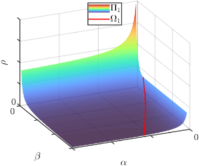
Figure 2: The trends of $\|T_{1}(s)\|_{\infty}$ with respect to $\alpha$ and $\beta$.

3.2 Anti-disturbance capability of the second-order MAS using relative velocity information

The following theorem gives the analytic expression of the anti-capability of second-order MAS (3) with relative velocity protocol (5).

Theorem 2.

Consider MAS (3)-(5) in which $G$ is a connected undirected graph with $L$ being its Laplacian matrix. Then, we obtain

$$\|T_{2}(s)\|_{\infty}=\begin{dcases}\frac{1}{\sqrt{(\alpha\lambda_{2})^{2}-\Big{[}\sqrt{(\alpha\lambda_{2}+1)^{2}-(\beta\lambda_{2})^{2}}-1\Big{]}^{2}}},&\text{if}~{}~{}0<\beta<\sqrt{\alpha^{2}+\frac{2\alpha}{\lambda_{2}}},\\ \frac{1}{\alpha\lambda_{2}},&\text{if}~{}~{}\beta\geq\sqrt{\alpha^{2}+\frac{2\alpha}{\lambda_{2}}}.\end{dcases}$$ (22)

Proof 3.

Since the undirected graph $\mathcal{G}$ is connected, it follows from Lemma 2 that there exists an orthogonal matrix $Q\in\mathbb{R}^{n\times n}$ such that (1) and (2) hold. Then performing the orthogonal transformation (13) for the system (10) yields

$$\begin{dcases}\begin{bmatrix}\dot{\hat{x}}(t)\\ \dot{\hat{v}}(t)\end{bmatrix}=\begin{bmatrix}\mathbf{0}&I_{n}\\ -\alpha\bar{L}&-\beta\bar{L}\end{bmatrix}\begin{bmatrix}\hat{x}(t)\\ \hat{v}(t)\end{bmatrix}+\begin{bmatrix}\mathbf{0}\\ I_{n}\end{bmatrix}\hat{\omega}(t),\\ \hat{y}(t)=\begin{bmatrix}\bar{\Phi}_{n}&\mathbf{0}\\ \mathbf{0}&\bar{\Phi}_{n}\end{bmatrix}\begin{bmatrix}\hat{x}(t)\\ \hat{v}(t)\end{bmatrix},\end{dcases}$$ (23)

where

$$\bar{L}=\begin{bmatrix}\bar{L}_{1}&\mathbf{0}_{n-1}\\ \mathbf{0}_{n-1}^{\top}&0\end{bmatrix}.$$

It is observed from Lemma 1 and (2) that positive definite matrix $\bar{L}_{1}$ owns the same non-zero eigenvalues of $L$ which implies that $-\bar{L}_{1}$ is Hurwitz stable. Obviously, the system (23) is decomposed into an observable asymptotically stable subsystem of order $2n-2$ and an unobservable marginally stable subsystem of order $2$. According to [35], $\|T_{2}(s)\|_{\infty}$ is well-defined and completely reliant on the asymptotically stable subsystem. Thus we turn to analyze the asymptotically stable subsystem of (23) which is given as follows

$$\begin{dcases}\begin{bmatrix}\dot{\hat{x}}^{1}(t)\\ \dot{\hat{v}}^{1}(t)\end{bmatrix}=\begin{bmatrix}\mathbf{0}&I_{n-1}\\ -\alpha\bar{L}_{1}&-\beta\bar{L}_{1}\end{bmatrix}\begin{bmatrix}\hat{x}^{1}(t)\\ \hat{v}^{1}(t)\end{bmatrix}+\begin{bmatrix}\mathbf{0}\\ I_{n-1}\end{bmatrix}\hat{\omega}^{1}(t),\\ \hat{y}^{1}(t)=\begin{bmatrix}I_{n-1}&\mathbf{0}\\ \mathbf{0}&I_{n-1}\end{bmatrix}\begin{bmatrix}\hat{x}^{1}(t)\\ \hat{v}^{1}(t)\end{bmatrix},\end{dcases}$$ (24)

where $\hat{x}^{1}(t)=\begin{bmatrix}I_{n-1}&\mathbf{0}_{n-1}\end{bmatrix}\hat{x}(t)$, $\hat{v}^{1}(t)=\begin{bmatrix}I_{n-1}&\mathbf{0}_{n-1}\end{bmatrix}$   $\hat{v}(t)$ and $\hat{\omega}^{1}(t)=\begin{bmatrix}I_{n-1}&\mathbf{0}_{n-1}\end{bmatrix}\hat{\omega}(t).$ Since $\bar{L}_{1}$ is positive definite, there must exists an orthogonal matrix $V\in\mathbb{R}^{(n-1)\times(n-1)}$ such that $V^{\top}\bar{L}_{1}V=\varLambda$, where $\varLambda=\text{diag}\{\lambda_{2},\lambda_{3},\dots,\lambda_{n}\}$. Then applying the orthogonal transformation (16) for system (24) elicits the following system

$$\begin{dcases}\begin{bmatrix}\dot{\tilde{x}}(t)\\ \dot{\tilde{v}}(t)\end{bmatrix}=\begin{bmatrix}\mathbf{0}&I_{n-1}\\ -\alpha\varLambda&-\beta\varLambda\end{bmatrix}\begin{bmatrix}\tilde{x}(t)\\ \tilde{v}(t)\end{bmatrix}+\begin{bmatrix}\mathbf{0}\\ I_{n-1}\end{bmatrix}\tilde{\omega}(t),\\ \tilde{y}(t)=\begin{bmatrix}I_{n-1}&\mathbf{0}\\ \mathbf{0}&I_{n-1}\end{bmatrix}\begin{bmatrix}\tilde{x}(t)\\ \tilde{v}(t)\end{bmatrix}.\end{dcases}$$ (25)

We indicate the transfer matrix of the system (23), (24) and (25) by $T_{6}(s)$, $T_{7}(s)$ and $T_{8}(s)$, respectively. A simple calculation gives rise to

$$\|T_{2}(s)\|_{\infty}=\|T_{6}(s)\|_{\infty}=\|T_{7}(s)\|_{\infty}=\|T_{8}(s)\|_{\infty}.$$ (26)

Next, we intend to compute $\|T_{8}(s)\|_{\infty}$.

The transfer matrix $T_{8}(s)$ is given as

$$T_{8}(s)=\left[\begin{array}[]{ccc}\Psi_{2}&&\\ &\ddots&\\ &&\Psi_{n}\\ \hdashline\Omega_{2}&&\\ &\ddots&\\ &&\Omega_{n}\end{array}\right],$$

where $\Psi_{i}=\dfrac{1}{s^{2}+\beta\lambda_{i}s+\alpha\lambda_{i}}$ and $\Omega_{i}=\dfrac{s}{s^{2}+\beta\lambda_{i}s+\alpha\lambda_{i}}$, $i=2,\dots,n$. We can obtain that

$$T_{8}^{H}(\mathbf{j}\upsilon)T_{8}(\mathbf{j}\upsilon)=\begin{bmatrix}\theta_{2}(\upsilon)&&\\ &\ddots&\\ &&\theta_{n}(\upsilon)\end{bmatrix}$$

is diagonal, where

$$\theta_{i}(\upsilon)=\frac{1+\upsilon^{2}}{(\alpha\lambda_{i}-\upsilon^{2})^{2}+(\beta\lambda_{i}\upsilon)^{2}}>0,~{}i=2,\dots,n,~{}\upsilon\in\mathbb{R}.$$

By inspecting Definition 2 and (26), $\|T_{2}(s)\|_{\infty}$ can be written as

$$\begin{split}\|T_{2}(s)\|_{\infty}&=\|T_{8}(s)\|_{\infty}\\ &=\sup_{\upsilon\in\mathbb{R}}\sqrt{\lambda_{max}\big{[}T_{8}^{H}(\mathbf{j}\upsilon)T_{8}(\mathbf{j}\upsilon)\big{]}}\\ &=\max_{i=2,\dots,n}\sqrt{\sup_{\upsilon\in\mathbb{R}}\theta_{i}(\upsilon)}.\end{split}$$ (27)

It follows from

$$\frac{\mathrm{d}\theta_{i}(\upsilon)}{\mathrm{d}\upsilon}=\frac{-2\upsilon\big{[}\upsilon^{4}+2\upsilon^{2}+\beta^{2}\lambda_{i}^{2}-(\alpha\lambda_{i})^{2}-2\alpha\lambda_{i}\big{]}}{\big{[}\upsilon^{4}+(\beta^{2}\lambda_{i}^{2}-2\alpha\lambda_{i})\upsilon^{2}+(\alpha\lambda_{i})^{2}\big{]}^{2}}=0$$ (28)

that

$$\upsilon\big{[}\upsilon^{4}+2\upsilon^{2}+\beta^{2}\lambda_{i}^{2}-(\alpha\lambda_{i})^{2}-2\alpha\lambda_{i}\big{]}=0.$$ (29)

Obviously, $\sup_{\upsilon\in\mathbb{R}}\theta_{i}(\upsilon)$ is determined by $\beta^{2}\lambda_{i}^{2}-2\alpha\lambda_{i}-\alpha^{2}\lambda_{i}^{2}$. If $\beta\geq\sqrt{\alpha^{2}+\frac{2\alpha}{\lambda_{i}}}$, by solving (29), we get

$$\sup_{\upsilon\in\mathbb{R}}\theta_{i}(\upsilon)=\theta_{i}(\upsilon^{*}_{i,1})=g_{1}{(\lambda_{i})}=\frac{1}{(\alpha\lambda_{i})^{2}},$$

where $\upsilon^{*}_{i,1}=0$. If $\beta<\sqrt{\alpha^{2}+\frac{2\alpha}{\lambda_{i}}}$, by solving (29), we obtain

$$\sup_{\upsilon\in\mathbb{R}}\theta_{i}(\upsilon) =\theta_{i}(\upsilon^{*}_{i,2})=\theta_{i}(\upsilon^{*}_{i,3})=g_{3}{(\lambda_{i})}$$

$$=\frac{1}{(\alpha\lambda_{i})^{2}-(\sqrt{\Theta_{i}}-1)^{2}},$$

where $\upsilon^{*}_{i,2},\upsilon^{*}_{i,3}=\pm\sqrt{\sqrt{\Theta_{i}}-1}$, and $\Theta_{i}=(\alpha\lambda_{i}+1)^{2}-(\beta\lambda_{i})^{2}$. The trends of the function $\theta_{i}(\upsilon)$ under the conditions $\beta\geq\sqrt{\alpha^{2}+\frac{2\alpha}{\lambda_{i}}}$ and $\beta<\sqrt{\alpha^{2}+\frac{2\alpha}{\lambda_{i}}}$ resemble the Fig. 1. For saving space, we omit it here.

Aforementioned analysis prompts us to dictate two sets of non-zero eigenvalues of $L$, which are given as

$$\mathcal{K}_{1}=\Bigg{\{}k\in\Gamma~{}\bigg{|}~{}\beta\geq\sqrt{\alpha^{2}+\frac{2\alpha}{k}}\Bigg{\}}$$

and

$$\mathcal{K}_{2}=\Bigg{\{}k\in\Gamma~{}\bigg{|}~{}\beta<\sqrt{\alpha^{2}+\frac{2\alpha}{k}}\Bigg{\}}.$$

Obviously, we can get $\mathcal{K}_{1}\cup\mathcal{K}_{2}=\Gamma$ and $\mathcal{K}_{1}\cap\mathcal{K}_{2}=\emptyset$. We will complete the proof by enumeration.

(I) $\mathcal{K}_{1}=\Gamma$ and $\mathcal{K}_{2}=\emptyset$;

In this case, we have $\beta\geq\sqrt{\alpha^{2}+\frac{2\alpha}{\lambda_{i}}},\forall i\in\{2,\dots,n\}$ which implies that $\sup_{\upsilon\in\mathbb{R}}\theta_{i}(\upsilon)=g_{1}{(\lambda_{i})},\forall i\in\{2,\dots,n\}$. Because $0<\lambda_{2}\leq\cdots\leq\lambda_{n}$ and $g_{1}{(t)}$ is decreasing on $(0,+\infty)$, one can obtain that $\max_{i=2,\dots,n}g_{1}{(\lambda_{i})}=g_{1}(\lambda_{2})$. Then (27) becomes

$$\|T_{2}(s)\|_{\infty}=\max_{i=2,\dots,n}\sqrt{g_{1}{(\lambda_{i})}}=\sqrt{g_{1}(\lambda_{2})}=\frac{1}{\alpha\lambda_{2}}.$$

(II) $\mathcal{K}_{1}=\emptyset$ and $\mathcal{K}_{2}=\Gamma$;

In this case, we get $\beta<\sqrt{\alpha^{2}+\frac{2\alpha}{\lambda_{i}}},\forall i\in\{2,\dots,n\}$ which leads to $\sup_{\upsilon\in\mathbb{R}}\theta_{i}(\upsilon)=g_{3}{(\lambda_{i})},\forall i\in\{2,\dots,n\}$. If $\beta\leq\alpha$, it is inferred from $0<\lambda_{2}\leq\cdots\leq\lambda_{n}$ and Lemma 3 that

$$\max_{i=2,\dots,n}g_{3}{(\lambda_{i})}=g_{3}(\lambda_{2}).$$ (30)

If $\beta>\alpha$, it follows from $0<\lambda_{2}\leq\cdots\leq\lambda_{n}$ and $\beta<\sqrt{\alpha^{2}+\frac{2\alpha}{\lambda_{i}}},\forall i\in\{2,\dots,n\}$ that $0<\lambda_{2}\leq\cdots\leq\lambda_{n}<\frac{2\alpha}{\beta^{2}-\alpha^{2}}$. Then according to Lemma 3, equation (30) still holds. Building on above analysis, no matter $\beta\leq\alpha$ or $\beta>\alpha$, (27) can be written as

$$\begin{split}\|T_{2}(s)\|_{\infty}&=\max_{i=2,\dots,n}\sqrt{g_{3}{(\lambda_{i})}}\\ &=\sqrt{g_{3}(\lambda_{2})}\\ &=\frac{1}{\sqrt{(\alpha\lambda_{2})^{2}-\Big{[}\sqrt{(\alpha\lambda_{2}+1)^{2}-(\beta\lambda_{2})^{2}}-1\Big{]}^{2}}}.\end{split}$$

(III) $\mathcal{K}_{1}\neq\emptyset$ and $\mathcal{K}_{2}\neq\emptyset$.

Under this circumstance, there must exists an eigenvalue $\lambda_{m}$ $(2\leq m\leq n-1)$ of $L$ such that $\mathcal{K}_{1}=\{\lambda_{m+1},\dots,\lambda_{n}\}$ and $\mathcal{K}_{2}=\{\lambda_{2},\dots,\lambda_{m}\}$. Then we have $\beta\geq\sqrt{\alpha^{2}+\frac{2\alpha}{\lambda_{i}}},\forall i\in\{m+1,\dots,n\}$ and $\beta<\sqrt{\alpha^{2}+\frac{2\alpha}{\lambda_{i}}},\forall i\in\{2,\dots,m\}$ which respectively lead to $\sup_{\upsilon\in\mathbb{R}}\theta_{i}(\upsilon)=g_{1}{(\lambda_{i})},\forall i\in\{m+1,\dots,n\}$ and $\sup_{\upsilon\in\mathbb{R}}\theta_{i}(\upsilon)=g_{3}{(\lambda_{i})},\forall i\in\{2,\dots,m\}$. Since $0<\lambda_{m+1}\leq\cdots\leq\lambda_{n}$ and $g_{1}{(t)}$ is decreasing on $(0,+\infty)$, one can obtain that $\max_{i=m+1,\dots,n}g_{1}{(\lambda_{i})}=g_{1}(\lambda_{m+1})$. Furthermore, it can be readily concluded that

$$\alpha<\sqrt{\alpha^{2}+\dfrac{2\alpha}{\lambda_{n}}}\leq\dots\leq\sqrt{\alpha^{2}+\dfrac{2\alpha}{\lambda_{m+1}}}\leq\beta.$$

Since $\alpha<\beta$, it follows from $0<\lambda_{2}\leq\cdots\leq\lambda_{m}$ and $\beta<\sqrt{\alpha^{2}+\frac{2\alpha}{\lambda_{i}}},\forall i\in\{2,\dots,m\}$ that $0<\lambda_{2}\leq\cdots\leq\lambda_{m}<\frac{2\alpha}{\beta^{2}-\alpha^{2}}$. According to Lemma 3, we can obtain $\max_{i=2,\dots,m}g_{3}{(\lambda_{i})}=g_{3}(\lambda_{2})$.

Based on above analysis, (27) can be written as

$$\|T_{2}(s)\|_{\infty}= \max\bigg{\{}\max_{i=m+1,\dots,n}\sqrt{g_{1}{(\lambda_{i})}},\max_{i=2,\dots,m}\sqrt{g_{3}{(\lambda_{i})}}\bigg{\}}$$

$$= \max\Big{\{}\sqrt{g_{1}(\lambda_{m+1})},\sqrt{g_{3}(\lambda_{2})}\Big{\}}$$

It follows from $\beta<\sqrt{\alpha^{2}+\frac{2\alpha}{\lambda_{2}}}$ and $\lambda_{m+1}\geq\lambda_{2}$ that

$$\begin{split}g_{3}(\lambda_{2})=&\frac{1}{(\alpha\lambda_{2})^{2}-\Big{[}\sqrt{(\alpha\lambda_{2}+1)^{2}-(\beta\lambda_{2})^{2}}-1\Big{]}^{2}}\\ >&\frac{1}{(\alpha\lambda_{2})^{2}}\geq\frac{1}{(\alpha\lambda_{m+1})^{2}}=g_{1}(\lambda_{m+1}).\end{split}$$

Therefore, we can obtain

$$\|T_{2}(s)\|_{\infty}=\sqrt{g_{3}(\lambda_{2})}=\frac{1}{\sqrt{(\alpha\lambda_{2})^{2}-\Big{[}\sqrt{(\alpha\lambda_{2}+1)^{2}-(\beta\lambda_{2})^{2}}-1\Big{]}^{2}}}$$

To summarize above cases, we can conclude that

$$\|T_{2}(s)\|_{\infty}=\frac{1}{\sqrt{(\alpha\lambda_{2})^{2}-\Big{[}\sqrt{(\alpha\lambda_{2}+1)^{2}-(\beta\lambda_{2})^{2}}-1\Big{]}^{2}}}$$

as long as $\lambda_{2}\in\mathcal{K}_{2}$, i.e., $\beta<\sqrt{\alpha^{2}+\frac{2\alpha}{\lambda_{2}}}$. Otherwise, $\|T_{2}(s)\|_{\infty}=\frac{1}{\alpha\lambda_{2}}$. That is to say, (22) is obtained. $\square$

In fact, $\|T_{2}(s)\|_{\infty}$ can be deemed as a continuous function of the two variables $\alpha\in\mathbb{R}^{+}$ and $\beta\in\mathbb{R}^{+}$ on a given connected undirected graph $\mathcal{G}$. We roughly portray the two-dimensional surface $\Pi_{2}:=\Big{\{}(\alpha,\beta,\rho)\in\mathbb{R}^{3}~{}\big{|}~{}\alpha\in\mathbb{R}^{+},\beta\in\mathbb{R}^{+},\rho=\|T_{2}(s)\|_{\infty}\Big{\}}$ of $\|T_{2}(s)\|_{\infty}$ with respect to $\alpha$ and $\beta$ in Fig. 3. As one can see from Fig. 3, $\Pi_{2}$ is seperated into two regions by the yellow solid curve

$$\Omega_{2}:=\Bigg{\{}(\alpha,\beta,\rho)\in\Pi_{2}~{}\bigg{|}~{}\beta=\sqrt{\alpha^{2}+\dfrac{2\alpha}{\lambda_{2}}}\Bigg{\}},$$

which refers to the critical condition in (22).

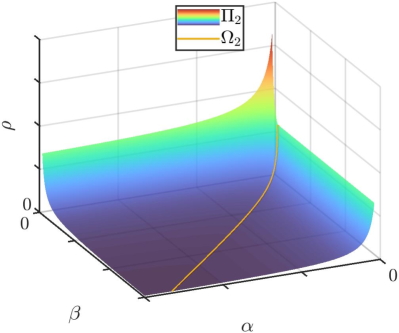
Figure 3: The trends of $\|T_{2}(s)\|_{\infty}$ with respect to $\alpha$ and $\beta$.

Remark 1.

It is observed from Theorem 1 and Theorem 2 that $\|T_{1}(s)\|_{\infty}$ and $\|T_{2}(s)\|_{\infty}$ are both inversely proportional to $\lambda_{2}$ for any given tunable gains, which is consistent with the result for first-order MASs [28]. In other words, optimizing networks to generate a larger $\lambda_{2}$ is still valid to improve the anti-disturbance capability for second-order MASs.

3.3 Protocol selection for better anti-disturbance capability

According to the analytic expressions presented in Theorems 1 and 2, in Theorem 3 we will establish the graph conditions of protocol selection for better anti-disturbance capability.

Theorem 3.

Consider the second-order MAS (3) on a connected undirected graph $\mathcal{G}$ with Laplacian matrix $L$. Then, we conclude that

• The protocol (4) outperforms the protocol (5) if $\lambda_{2}<1$;

• The protocol (5) outperforms the protocol (4) if $\lambda_{2}>1$;

• The protocol (4) performs as well as the protocol (5) if $\lambda_{2}=1$.

Proof 4.

Firstly, we intend to prove the conclusion 3). By substituting $\lambda_{2}=1$ into (12) and (22), respectively, it is easy to verify that $\|T_{1}(s)\|_{\infty}\equiv\|T_{2}(s)\|_{\infty}$ for any $\alpha>0$ and $\beta>0$. Therefore, according to Definition 4, we can say that the protocol (4) performs as well as the protocol (5).

Next, we will prove the conclusion 1). Let $p=\sqrt{(\alpha\lambda_{2})^{2}+2\alpha\lambda_{2}}$ and $q=\sqrt{\alpha^{2}+\frac{2\alpha}{\lambda_{2}}}$. Note that $p=\lambda_{2}q$. Recall that $\Delta_{2}=(\alpha\lambda_{2}+1)^{2}-\beta^{2}$ and $\Theta_{2}=(\alpha\lambda_{2}+1)^{2}-(\beta\lambda_{2})^{2}$. It follows from $\lambda_{2}<1$ that $p<q$ and $\Delta_{2}<\Theta_{2}$. We will complete the proof of conclusion 1) by enumeration.

(I) $\beta<p<q$;

As seen in Theorem 1 and Theorem 2, we can obtain

$$\|T_{1}(s)\|_{\infty}=\frac{1}{\sqrt{(\alpha\lambda_{2})^{2}-(\sqrt{\Delta_{2}}-1)^{2}}}$$

and

$$\|T_{2}(s)\|_{\infty}=\frac{1}{\sqrt{(\alpha\lambda_{2})^{2}-(\sqrt{\Theta_{2}}-1)^{2}}}.$$

Since $\beta<p$ and $\Delta_{2}<\Theta_{2}$, we have $1<\Delta_{2}<\Theta_{2}$. It follows that

$$\sqrt{(\alpha\lambda_{2})^{2}-(\sqrt{\Theta_{2}}-1)^{2}}<\sqrt{(\alpha\lambda_{2})^{2}-(\sqrt{\Delta_{2}}-1)^{2}}$$

which means that $\|T_{1}(s)\|_{\infty}<\|T_{2}(s)\|_{\infty}$.

(II) $p\leq\beta<q$;

In terms of Theorem 1 and Theorem 2, one can obtain that $\|T_{1}(s)\|_{\infty}=\frac{1}{\alpha\lambda_{2}}$ and

$$\|T_{2}(s)\|_{\infty}=\frac{1}{\sqrt{(\alpha\lambda_{2})^{2}-(\sqrt{\Theta_{2}}-1)^{2}}}.$$

It is inferred from

$$\sqrt{(\alpha\lambda_{2})^{2}-(\sqrt{\Theta_{2}}-1)^{2}}<\sqrt{(\alpha\lambda_{2})^{2}}$$

that $\|T_{1}(s)\|_{\infty}<\|T_{2}(s)\|_{\infty}$.

(III) $p<q\leq\beta$.

It follows from Theorem 1 and Theorem 2 that $\|T_{1}(s)\|_{\infty}=\|T_{2}(s)\|_{\infty}=\frac{1}{\alpha\lambda_{2}}$.

In summary, $\|T_{1}(s)\|_{\infty}\leq\|T_{2}(s)\|_{\infty}$ holds for any $\alpha>0$ and $\beta>0$ when $\lambda_{2}<1$. Therefore, as stated in Definition 4, we can say that the protocol (4) outperforms the protocol (5) if $\lambda_{2}<1$. Similarly, if $\lambda_{2}>1$, we can also conclude that the protocol (5) outperforms the protocol (4). For saving space, we omit it. $\square$

As one can see, the protocol selection for better anti-disturbance capability exclusively relies on the graph-theoretic feature $\lambda_{2}$. It means that we do not have to execute complicated calculation and comparison on $\|T_{1}(s)\|_{\infty}$ and $\|T_{2}(s)\|_{\infty}$ for all positive tunable gains $\alpha$ and $\beta$ as Definition 4, the graph conditions about $\lambda_{2}$ are more consice and tractable.

Additionally, our results embody a twofold approach for improving the anti-disturbance capability of MAS (3). In a fixed communication network scenario, we can first opt for a better communication protocol in terms of Theorem 3. Then the importance of the tunable gains $\alpha$ and $\beta$ now comes to the fore. As shown in (12) and (22), $\|T_{1}(s)\|_{\infty}$ and $\|T_{2}(s)\|_{\infty}$ can be viewed as the functions of tunable gains $\alpha$ and $\beta$. Note that the partial derivatives $\frac{\partial\|T_{1}(s)\|_{\infty}}{\partial\alpha}$, $\frac{\partial\|T_{1}(s)\|_{\infty}}{\partial\beta}$, $\frac{\partial\|T_{2}(s)\|_{\infty}}{\partial\alpha}$ and $\frac{\partial\|T_{2}(s)\|_{\infty}}{\partial\beta}$ are all continuous, and we have

$$\begin{dcases}\dfrac{\partial\|T_{1}(s)\|_{\infty}}{\partial\alpha}<0,\dfrac{\partial\|T_{2}(s)\|_{\infty}}{\partial\alpha}<0,\\ \dfrac{\partial\|T_{1}(s)\|_{\infty}}{\partial\beta}\leq 0,\dfrac{\partial\|T_{2}(s)\|_{\infty}}{\partial\beta}\leq 0,\end{dcases}$$

where the equations $\frac{\partial\|T_{1}(s)\|_{\infty}}{\partial\beta}=0$ and $\frac{\partial\|T_{2}(s)\|_{\infty}}{\partial\beta}=0$ hold if and only if $\beta\geq\sqrt{(\alpha\lambda_{2})^{2}+2\alpha\lambda_{2}}$ and $\beta\geq\sqrt{\alpha^{2}+\frac{2\alpha}{\lambda_{2}}}$, respectively. Therefore, we are able to further improve the anti-disturbance capability by increasing the tunable gain $\alpha$ or $\beta$, which is also illustrated in Fig. 2 and Fig. 3. Nevertheless, on account of

$$\begin{gathered}\lim\limits_{\alpha\to\infty}\|T_{1}(s)\|_{\infty}=\dfrac{1}{\beta},\lim\limits_{\beta\to\infty}\|T_{1}(s)\|_{\infty}=\dfrac{1}{\alpha\lambda_{2}},\\ \lim\limits_{\alpha\to\infty}\|T_{2}(s)\|_{\infty}=\dfrac{1}{\beta\lambda_{2}},\lim\limits_{\beta\to\infty}\|T_{2}(s)\|_{\infty}=\dfrac{1}{\alpha\lambda_{2}},\end{gathered}$$

adjusting single tunable gain to improve anti-disturbance capability is limited. Consequently, the optimal anti-disturbance capability is obtained when both tunable gains are sufficiently large.

Remark 2.

The protocol selection approach embodies potential advantages in practical applications. Specifically, if the network is unable to rearrange or expand which means that modifying the network to improve the anti-disturbance capability is impracticable, we can still optimize the anti-disturbance capability by manipulating every agents to follow the identical optimal communication protocol. Moreover, for a certain control task of a MAS, selecting from existing practicable protocols rather than designing a new protocol is more tractable and highly efficient in the distributed scenario.

4 Simlulations

We provide simulations to illustrate the effectiveness of our theoretical results.

Consider the following well-known graphs with $n\geq 2$ vertices and $0$-$1$ edge weights, which include undirected complete graphs $K_{n}$, undirected star graphs $S_{n}$, undirected path graphs $P_{n}$, and undirected $2k$-regular ring lattices $C_{k,n}$. It should be stressed that $C_{k,n}$ $(n\geq 2k+1)$ are highly structured networks with nodes placed on a ring, each connecting to its $2k$ nearest neighbors. For more details about those networks, one can refer to [36, 37]. For above networks, Table 1 gives the analytic expressions of the minimum non-zero eigenvalue and the network density.

(a) $P_{4}$ with $\lambda_{2}=0.5858$

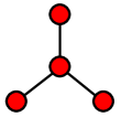
(b) $S_{4}$ with $\lambda_{2}=1$

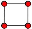
(c) $C_{1,4}$ with $\lambda_{2}=2$

Figure 4: Diagrams of $P_{4}$, $S_{4}$, and $C_{1,4}$.

Table 1: The analytic expressions of the minimum non-zero eigenvalue and the network density.

Graph	Value of $\lambda_{2}$	Network density $d$	$\lambda_{2}<1$	$\lambda_{2}=1$	$\lambda_{2}>1$
$K_{n}$	$\lambda_{2}=n$	$d=1$	✗	✗	$n\geq 2$
$S_{n}$	$\lambda_{2}=1~{}(n\geq 3)$	$d=\frac{2}{n}$	✗	$n\geq 3$	$n=2$
	$\lambda_{2}=2~{}(n=2)$
$P_{n}$	$\lambda_{2}=4\sin^{2}(\dfrac{\pi}{2n})$	$d=\frac{2}{n}$	$n>3$	$n=3$	$n=2$
$C_{1,n}$	$\lambda_{2}=3-\dfrac{\sin\frac{3\pi}{n}}{\sin\frac{\pi}{n}}$	$d=\frac{2}{n-1}$	$n\geq 7$	$n=6$	$n\leq 5$
$C_{2,n}$	$\lambda_{2}=5-\dfrac{\sin\frac{5\pi}{n}}{\sin\frac{\pi}{n}}$	$d=\frac{4}{n-1}$	$n\geq 14$	✗	$n\leq 13$
$C_{3,n}$	$\lambda_{2}=7-\dfrac{\sin\frac{7\pi}{n}}{\sin\frac{\pi}{n}}$	$d=\frac{6}{n-1}$	$n\geq 24$	✗	$n\leq 23$

In simulations, we will use three graphs $P_{4}$, $S_{4}$ and $C_{1,4}$, whose diagrams are depicted in Fig. 4, to illustrate our findings. For each network in Fig. 4, the two-dimensional surface $\Pi:=\Big{\{}(\alpha,\beta,\rho)\in\mathbb{R}^{3}~{}\big{|}~{}\alpha\in\mathbb{R}^{+},\beta\in\mathbb{R}^{+},\rho=\|T_{1}(s)\|_{\infty}-\|T_{2}(s)\|_{\infty}\Big{\}}$ is displayed in Fig. 5, which denotes the trends of difference between $\|T_{1}(s)\|_{\infty}$ and $\|T_{2}(s)\|_{\infty}$ with respect to tunable gains $\alpha$ and $\beta$. We respectively depict the red solid curve

$$\Sigma_{1}:=\Big{\{}(\alpha,\beta,\rho)\in\Pi~{}\big{|}~{}\beta=\sqrt{(\alpha\lambda_{2})^{2}+2\alpha\lambda_{2}}\Big{\}}$$

and the yellow dash curve

$$\Sigma_{2}:=\Bigg{\{}(\alpha,\beta,\rho)\in\Pi~{}\bigg{|}~{}\beta=\sqrt{\alpha^{2}+\dfrac{2\alpha}{\lambda_{2}}}\Bigg{\}}.$$

on $\Pi$ to emphasize the critical conditions in (12) and (22).

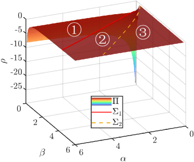
(a) The trends of $\|T_{1}(s)\|_{\infty}-\|T_{2}(s)\|_{\infty}$ for graph $P_{4}$

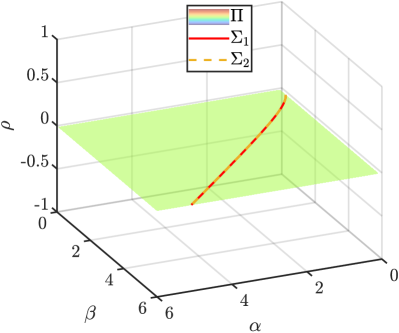
(b) The trends of $\|T_{1}(s)\|_{\infty}-\|T_{2}(s)\|_{\infty}$ for graph $S_{4}$

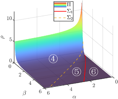
(c) The trends of $\|T_{1}(s)\|_{\infty}-\|T_{2}(s)\|_{\infty}$ for graph $C_{1,4}$

Figure 5: The trends of $\|T_{1}(s)\|_{\infty}-\|T_{2}(s)\|_{\infty}$ with respect to tunable gains $\alpha$ and $\beta$ for the graphs $P_{4}$, $S_{4}$ and $C_{1,4}$.

As one can see from Fig. 5a, the surface $\Pi$ is divided into three regions ①, ② and ③ by curves $\Sigma_{1}$ and $\Sigma_{2}$, which correspond to the three cases (I), (II) and (III) in the proof of Theorem 3, respectively. Obviously, the two regions ① and ② are always below the plane $\rho=0$ which means that $\|T_{1}(s)\|_{\infty}<\|T_{2}(s)\|_{\infty}$. While the region ③ completely overlaps the plane $\rho=0$ which implies that $\|T_{1}(s)\|_{\infty}=\|T_{2}(s)\|_{\infty}$. According to Definition 4, these observations tells that the absolute velocity protocol (4) is superior to the relative velocity protocol (5) when $\lambda_{2}<1$, which are in accordance with the conclusion 1) in Theorem 3. Likewise, as shown in Fig. 5c, the surface $\Pi$ is separated into three regions ④, ⑤ and ⑥ by curves $\Sigma_{1}$ and $\Sigma_{2}$. Obviously, bounded by the red solid line, the two regions ④ and ⑤ are always above the plane $\rho=0$ which means that $\|T_{1}(s)\|_{\infty}>\|T_{2}(s)\|_{\infty}$. While the region ⑥ completely overlaps the plane $\rho=0$ which implies that $\|T_{1}(s)\|_{\infty}=\|T_{2}(s)\|_{\infty}$. Therefore, it follows from Definition 4 that the relative velocity protocol (5) surpasses the absolute velocity protocol (4) when $\lambda_{2}>1$, which is consistent with the conclusion 2) in Theorem 3. It is observed from Fig. 5b that when $\lambda_{2}=1$, then $\|T_{1}(s)\|_{\infty}\equiv\|T_{2}(s)\|_{\infty}$ because the surface $\Pi$ completely overlaps the plane $\rho=0$. In other words, the absolute velocity protocol (4) performs as well as the relative velocity protocol (5) when $\lambda_{2}=1$, which is consistent with the finding presented in Theorem 3.

Furthermore, according to Theorem 3 and Table 1, for the undirected complete graph with any number of nodes, the relative velocity protocol is preferable to the absolute velocity protocol. For the path graph with the number of nodes greater than 3, the absolute velocity protocol is superior to the relative one. When the star graph whose number of nodes is not less than 3 is considered, both the two protocols have the same anti-disturbance capability. For the $2$-regular ring lattice, $4$-regular ring lattice and $6$-regular ring lattice, the absolute velocity protocol outperforms the relative velocity protocol when the number of nodes is not less than 7, 14 and 24, respectively, and the relative velocity protocol is superior to the absolute one when the number of nodes is note greater than 5, 13 and 23, respectively. Particularly, for the $2$-regular ring lattice with 6 nodes, both the two protocols own the same anti-disturbance capability. Based on these observations, our graph conditions seem to be consistent with the variation of network density $d$ whose trends as increasing number of nodes $n$ is shown in Fig. 6.

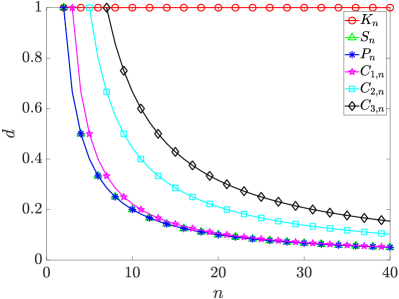
Figure 6: Trends of network density $d$ on various graphs.

In Fig. 6, the network density $d$ is diminishing with the growth in number of nodes except the complete graph which retains the highest density all through. Combining Fig. 6 with Theorem 3 and Table 1 obtains that the absolute velocity protocol (4) can be viewed as the optimal selection when the network density $d$ is not higher than a certain threshold, otherwise the relative velocity protocol (5) is always the best. And the threshold varies from different families of graphs.

5 Conclusion

In this paper, we investigated the anti-disturbance capability for the second-order MASs with absolute and relative velocity protocols, respectively, and gave the graph conditions to show which protocol owns better anti-disturbance capability. The anti-disturbance capability was characterized by the ${\mathcal{L}}_{2}\$gain from the disturbance to the consensus error. Firstly, we built the analytic expression of the ${\mathcal{L}}_{2}\$gain of the MAS with absolute velocity protocol. Then the analytic expression of the ${\mathcal{L}}_{2}\$gain of the MAS with relative velocity protocol was also established. It was shown that both the ${\mathcal{L}}_{2}\$gains for absolute and relative velocity protocols only depend on the minimum non-zero eigenvalue $\lambda_{2}$ of Laplacian matrix $L$ and the tunable gains $\alpha$ and $\beta$. Secondly, based on the analytic expressions of the ${\mathcal{L}}_{2}\$gain, we put forward the graph conditions for protocol selection for better anti-disturbance capability. It was proved that the absolute velocity protocol is superior to the relative velocity protocol if $\lambda_{2}<1$, and the relative velocity protocol outperforms the absolute one if $\lambda_{2}>1$. Especially, both the two protocols have the same anti-disturbance capability if $\lambda_{2}=1$. Moreover, we presented a two-step method for improving anti-disturbance capability. Finally, simulations illustrated the effectiveness of our findings. Although it might be intuitively true that the network density is associated with protocol selection, this fact deserves to be further verified in future works.

References

- [1] R. Olfati-Saber, J. A. Fax, R. M. Murray, Consensus and cooperation in networked multi-agent systems, Proceedings of the IEEE 95 (1) (2007) 215–233.
- [2] A. Jadbabaie, J. Lin, A. S. Morse, Coordination of groups of mobile autonomous agents using nearest neighbor rules, IEEE Transactions on Automatic Control 48 (6) (2003) 988–1001.
- [3] R. Olfati-Saber, R. Murray, Consensus problems in networks of agents with switching topology and time-delays, IEEE Transactions on Automatic Control 49 (9) (2004) 1520–1533.
- [4] W. Ren, R. W. Beard, Consensus seeking in multiagent systems under dynamically changing interaction topologies, IEEE Transactions on Automatic Control 50 (5) (2005) 655–661.
- [5] G. Xie, L. Wang, Consensus control for a class of networks of dynamic agents, International Journal of Robust and Nonlinear Control 17 (10-11) (2007) 941–959.
- [6] W. Ren, E. Atkins, Distributed multi-vehicle coordinated control via local information exchange, International Journal of Robust and Nonlinear Control 17 (10-11) (2007) 1002–1033.
- [7] J. Zhu, Y.-P. Tian, J. Kuang, On the general consensus protocol of multi-agent systems with double-integrator dynamics, Linear Algebra and its Applications 431 (5-7) (2009) 701–715.
- [8] W. Yu, G. Chen, M. Cao, Some necessary and sufficient conditions for second-order consensus in multi-agent dynamical systems, Automatica 46 (6) (2010) 1089–1095.
- [9] J. Mei, W. Ren, J. Chen, Distributed consensus of second-order multi-agent systems with heterogeneous unknown inertias and control gains under a directed graph, IEEE Transactions on Automatic Control 61 (8) (2015) 2019–2034.
- [10] P. Lin, Y. Jia, Consensus of second-order discrete-time multi-agent systems with nonuniform time-delays and dynamically changing topologies, Automatica 45 (9) (2009) 2154–2158.
- [11] J. Qin, H. Gao, W. X. Zheng, Second-order consensus for multi-agent systems with switching topology and communication delay, Systems & Control Letters 60 (6) (2011) 390–397.
- [12] W. Hou, M. Fu, H. Zhang, Z. Wu, Consensus conditions for general second-order multi-agent systems with communication delay, Automatica 75 (2017) 293–298.
- [13] X. Ai, S. Song, K. You, Second-order consensus of multi-agent systems under limited interaction ranges, Automatica 68 (2016) 329–333.
- [14] W. Zhu, H. Pu, D. Wang, H. Li, Event-based consensus of second-order multi-agent systems with discrete time, Automatica 79 (2017) 78–83.
- [15] S. M. Dibaji, H. Ishii, Resilient consensus of second-order agent networks: Asynchronous update rules with delays, Automatica 81 (2017) 123–132.
- [16] Y. Zheng, Y. Zhu, L. Wang, Consensus of heterogeneous multi-agent systems, IET Control Theory & Applications 5 (16) (2011) 1881–1888.
- [17] Y. Zheng, Q. Zhao, J. Ma, L. Wang, Second-order consensus of hybrid multi-agent systems, Systems & Control Letters 125 (2019) 51–58.
- [18] Q. Zhao, Y. Zheng, Y. Zhu, Consensus of hybrid multi-agent systems with heterogeneous dynamics, International Journal of Control 93 (12) (2020) 2848–2858.
- [19] Y. Zhu, L. Zhou, Y. Zheng, J. Liu, S. Chen, Sampled-data based resilient consensus of heterogeneous multiagent systems, International Journal of Robust and Nonlinear Control 30 (17) (2020) 7370–7381.
- [20] P. Lin, Y. Jia, Robust consensus analysis of a class of second-order multi-agent systems with uncertainty, IET control theory & applications 3 (4) (2010) 487–498.
- [21] P. Li, K. Qin, M. Shi, Distributed robust rotating consensus control for directed networks of second-order agents with mixed uncertainties and time-delay, Neurocomputing 148 (2015) 332–339.
- [22] J. Han, H. Zhang, H. Jiang, Event-based consensus control for second-order leader-following multi-agent systems, Journal of the Franklin Institute 353 (18) (2016) 5081–5098.
- [23] W. Huang, Y. Huang, S. Chen, Robust consensus control for a class of second-order multi-agent systems with uncertain topology and disturbances, Neurocomputing 313 (2018) 426–435.
- [24] P. Lin, Y. Jia, L. Li, Distributed robust consensus control in directed networks of agents with time-delay, Systems & Control Letters 57 (8) (2008) 643–653.
- [25] Z. Li, Z. Duan, G. Chen, On and performance regions of multi-agent systems, Automatica 47 (4) (2011) 797–803.
- [26] Y. Liu, Y. Jia, consensus control for multi-agent systems with linear coupling dynamics and communication delays, International Journal of Systems Science 43 (1) (2012) 50–62.
- [27] J. Wang, Z. Duan, Z. Li, G. Wen, Distributed and consensus control in directed networks, IET Control Theory & Applications 8 (3) (2014) 193–201.
- [28] M. Siami, N. Motee, Systemic measures for performance and robustness of large-scale interconnected dynamical networks, in: 53rd IEEE Conference on Decision and Control (CDC), 2014, pp. 5119–5124.
- [29] M. Pirani, E. M. Shahrivar, B. Fidan, S. Sundaram, Robustness of leader–follower networked dynamical systems, IEEE Transactions on Control of Network Systems 5 (4) (2018) 1752–1763.
- [30] M. Pirani, H. Sandberg, K. H. Johansson, A graph-theoretic approach to the performance of leader–follower consensus on directed networks, IEEE Control Systems Letters 3 (4) (2019) 954–959.
- [31] X. Yang, J. Wang, Y. Tan, Robustness analysis of leader-follower consensus for multi-agent systems characterized by double integrators, Systems & Control Letters 61 (11) (2012) 1103–1115.
- [32] T. C. Silva, L. Zhao, Machine Learning in Complex Networks, Springer International Publishing Switzerland, 2016.
- [33] B. M. Chen, Robust and Control, Springer-Veriag London, 2000.
- [34] M. Pirani, E. Nekouei, H. Sandberg, K. H. Johansson, A game-theoretic framework for security-aware sensor placement problem in networked control systems, IEEE Transactions on Automatic Control 67 (7) (2022) 3699–3706.
- [35] M. Siami, N. Motee, Network sparsification with guaranteed systemic performance measures, IFAC-PapersOnLine 48 (22) (2015) 246–251.
- [36] F. L. Lewis, H. Zhang, K. Hengster-Movric, A. Das, Cooperative Control of Multi-Agent Systems: Optimal and Adaptive Design Approaches, Springer-Verlag London, 2014.
- [37] C. W. Wu, Synchronization in Complex Networks of Nonlinear Dynamical Systems, World Scientific Publishing Co. Pte. Ltd, 2007.