Abstract

We revisit the domain of off-policy policy optimization in RL from the perspective of coordinate ascent. One commonly-used approach is to leverage the off-policy policy gradient to optimize a surrogate objective – the total discounted in expectation return of the target policy with respect to the state distribution of the behavior policy. However, this approach has been shown to suffer from the distribution mismatch issue, and therefore significant efforts are needed for correcting this mismatch either via state distribution correction or a counterfactual method. In this paper, we rethink off-policy learning via Coordinate Ascent Policy Optimization (CAPO), an off-policy actor-critic algorithm that decouples policy improvement from the state distribution of the behavior policy without using the policy gradient. This design obviates the need for distribution correction or importance sampling in the policy improvement step of off-policy policy gradient. We establish the global convergence of CAPO with general coordinate selection and then further quantify the convergence rates of several instances of CAPO with popular coordinate selection rules, including the cyclic and the randomized variants of CAPO. We then extend CAPO to neural policies for a more practical implementation. Through experiments, we demonstrate that CAPO provides a competitive approach to RL in practice.

1 Introduction

Policy gradient (PG) has served as one fundamental principle of a plethora of benchmark reinforcement learning algorithms (Degris et al., 2012; Lillicrap et al., 2016; Gu et al., 2017a; Mnih et al., 2016). In addition to the empirical success, PG algorithms have recently been shown to enjoy provably global convergence guarantees in the on-policy settings, including the true gradient settings (Agarwal et al., 2019; Bhandari and Russo, 2019; Mei et al., 2020; Cen et al., 2022) and the Monte-Carlo stochastic gradient settings (Liu et al., 2020a; Mei et al., 2021). However, on-policy PG is known to suffer from data inefficiency and lack of exploration due to the tight coupling between the learned target policy and the sampled trajectories. As a result, in many cases, off-policy learning is preferred to achieve better exploration with an aim to either increase sample efficiency or address the committal behavior in the on-policy learning scenarios (Mei et al., 2021; Chung et al., 2021). To address this, the off-policy PG theorem (Degris et al., 2012; Imani et al., 2018; Maei, 2018) and the corresponding off-policy actor-critic methods, which are established to optimize a surrogate objective defined as the total discounted return of the target policy in expectation with respect to the state distribution of the behavior policy, has been proposed and widely adopted to decouple policy learning from trajectory sampling (Wang et al., 2017; Gu et al., 2017b; Chung et al., 2021; Ciosek and Whiteson, 2018; Espeholt et al., 2018).

Despite the better exploration capability, off-policy PG methods are subject to the following fundamental issues: (i) Correction for distribution mismatch: The standard off-policy PG methods resort to a surrogate objective, which ignores the mismatch between on-policy and the off-policy state distributions. Notably, it has been shown that such mismatch could lead to sub-optimal policies as well as poor empirical performance (Liu et al., 2020b). As a result, substantial efforts are needed to correct this distribution mismatch (Imani et al., 2018; Liu et al., 2020b; Zhang et al., 2020). (ii) Fixed behavior policy and importance sampling: The formulation of off-policy PG presumes the use of a static behavior policy throughout training as it is designed to optimize a surrogate objective with respect to the behavior policy. However, in many cases, we do prefer that the behavior policy varies with the target policy (e.g., epsilon-greedy exploration) as it is widely known that importance sampling could lead to significant variance in gradient estimation, especially when the behavior policy substantially deviates from the current policy. As a result, one fundamental research question that we would like to answer is: “How to achieve off-policy policy optimization with global convergence guarantees, but without the above limitations of off-policy PG?”

To answer this question, in this paper we take a different approach and propose an alternative off-policy policy optimization framework termed Coordinate Ascent Policy Optimization (CAPO), which revisits the policy optimization problem through the lens of coordinate ascent. Our key insight is that the distribution mismatch and the fixed behavior policy issues in off-policy PG both result from the tight coupling between the behavior policy and the objective function in policy optimization. To address this issue, we propose to still adopt the original objective of standard on-policy PG, but from the perspective of coordinate ascent with the update coordinates determined by the behavior policy. Through this design, we can completely decouple the objective function from the behavior policy while still enabling off-policy policy updates. Under the canonical tabular softmax parameterization, where each “coordinate" corresponds to a parameter specific to each state-action pair, CAPO iteratively updates the policy by performing coordinate ascent for those state-action pairs in the mini-batch, without resorting to the full gradient information or any gradient estimation. While being a rather simple method in the optimization literature, coordinate ascent and the resulting CAPO enjoy two salient features that appear rather useful in the context of RL:

• With the simple coordinate update, CAPO is capable of improving the policy by following any policy under a mild condition, directly enabling off-policy policy updates with an adaptive behavior policy. This feature addresses the issue of fixed behavior policy.

• Unlike PG, which requires having either full gradient information (the true PG setting) or an unbiased estimate of the gradient (the stochastic PG setting), updating the policy in a coordinate-wise manner allows CAPO to obviate the need for true gradient or unbiasedness while still retaining strict policy improvement in each update. As a result, this feature also obviates the need for distribution correction or importance sampling in the policy update.

To establish the global convergence of CAPO, we need to tackle the following main challenges: (i) In the coordinate descent literature, one common property is that the coordinates selected for the update are either determined according to a deterministic sequence (e.g., cyclic coordinate descent) or drawn independently from some distribution (e.g., randomized block coordinate descent) (Nesterov, 2012). By contrast, given the highly stochastic and non-i.i.d. nature of RL environments, in the general update scheme of CAPO, we impose no assumption on the data collection process, except for the standard condition of infinite visitation to each state-action pair (Singh et al., 2000; Munos et al., 2016). (ii) The function of total discounted expected return is in general non-concave, and the coordinate ascent methods could only converge to a stationary point under the general non-concave functions. Despite the above, we are able to show that the proposed CAPO algorithm attains a globally optimal policy with properly-designed step sizes under the canonical softmax parameterization. (iii) In the optimization literature, it is known that the coordinate ascent methods can typically converge slowly compared to the gradient counterpart. Somewhat surprisingly, we show that CAPO achieves comparable convergence rates as the true on-policy PG (Mei et al., 2020). Through our convergence analysis, we found that this can be attributed to the design of the state-action-dependent variable step sizes.

Built on the above results, we further generalize CAPO to the case of neural policy parameterization for practical implementation. Specifically, Neural CAPO (NCAPO) proceeds by the following two steps: (i) Given a mini-batch of state-action pairs, we leverage the tabular CAPO as a subroutine to obtain a collection of reference action distributions for those states in the mini-batch. (ii) By constructing a loss function (e.g., Kullback-Leibler divergence), we guide the policy network to update its parameters towards the state-wise reference action distributions. Such update can also be interpreted as solving a distributional regression problem.

Our Contributions. In this work, we revisit off-policy policy optimization and propose a novel policy-based learning algorithm from the perspective of coordinate ascent. The main contributions can be summarized as follows:

• We propose CAPO, a simple yet practical off-policy actor-critic framework with global convergence, and naturally enables direct off-policy policy updates with more flexible use of adaptive behavior policies, without the need for distribution correction or importance sampling correction to the policy gradient.

• We show that the proposed CAPO converges to a globally optimal policy under tabular softmax parameterization for general coordinate selection rules and further characterize the convergence rates of CAPO under multiple popular variants of coordinate ascent. We then extend the idea of CAPO to learning general neural policies to address practical RL settings.

• Through experiments, we demonstrate that NCAPO achieves comparable or better empirical performance than various popular benchmark methods in the MinAtar environment (Young and Tian, 2019).

Notations. Throughout the paper, we use $[n]$ to denote the set of integers $\{1,\cdots,n\}$. For any $x\in\mathbb{R}\backslash\{0\}$, we use $\operatorname{sign}(x)$ to denote $\frac{x}{\lvert x\rvert}$ and set $\operatorname{sign}(0)=0$. We use $\mathbb{I}\{\cdot\}$ to denote the indicator function.

2 Preliminaries

Markov Decision Processes. We consider an infinite-horizon Markov decision process (MDP) characterized by a tuple $(\operatorname{\mathcal{S}},\operatorname{\mathcal{A}},\mathcal{P},r,\gamma,\rho)$, where (i) $\mathcal{S}$ denotes the state space, (ii) $\operatorname{\mathcal{A}}$ denotes a finite action space, (iii) $\operatorname{\mathcal{P}}:\operatorname{\mathcal{S}}\times\operatorname{\mathcal{A}}\rightarrow\Delta(\operatorname{\mathcal{S}})$ is the transition kernel determining the transition probability $\mathcal{P}(s^{\prime}\rvert s,a)$ from each state-action pair $(s,a)$ to a next state $s^{\prime}$, where $\Delta(\operatorname{\mathcal{S}})$ is a probability simplex over $\operatorname{\mathcal{S}}$, (iv) $r:\mathcal{S}\times\mathcal{A}\rightarrow[0,1]$ is the reward function, (v) $\gamma\in(0,1)$ is the discount factor, and (vi) $\rho$ is the initial state distribution. In this paper, we consider learning a stationary parametric stochastic policy denoted as $\pi_{\theta}:\operatorname{\mathcal{S}}\rightarrow\Delta(\operatorname{\mathcal{A}})$, which specifies through a parameter vector $\theta$ the action distribution from a probability simplex $\Delta(\operatorname{\mathcal{A}})$ over $\operatorname{\mathcal{A}}$ for each state. For a policy $\pi_{\theta}$, the value function $V^{\pi_{\theta}}:\mathcal{S}\rightarrow\mathbb{R}$ is defined as the sum of discounted expected future rewards obtained by starting from state $s$ and following $\pi_{\theta}$, i.e.,

$$V^{\pi_{\theta}}(s):=\mathbb{E}\bigg{[}\sum_{t=0}^{\infty}\gamma^{t}r(s_{t},a_{t})\bigg{|}\pi_{\theta},s_{0}=s\bigg{]},$$ (1)

where $t$ represents the timestep of the trajectory $\{(s_{t},a_{t})\}^{\infty}_{t=0}$ induced by the policy $\pi_{\theta}$ with the initial state $s_{0}=s$. The goal of the learner is to search for a policy that maximizes the following objective function as

$$V^{\pi_{\theta}}(\rho):=\mathbb{E}_{s\sim\rho}[V^{\pi_{\mathbf{\theta}}}(s)].$$ (2)

For ease of exposition, we use $\pi^{*}$ to denote an optimal policy and let $V^{*}(s)$ be a shorthand notation for $V^{\pi^{*}}(s)$. Moreover, for any given policy $\pi_{\theta}$, we define the $Q$-function $Q^{\pi_{\theta}}:\mathcal{S}\times\mathcal{A}\rightarrow\mathbb{R}$ as

$$Q^{\pi_{\theta}}(s,a):=\mathbb{E}\bigg{[}\sum_{t=0}^{\infty}\gamma^{t}r(s_{t},a_{t})\bigg{|}\pi,s_{0}=s,a_{0}=a\bigg{]}.$$ (3)

We also define the advantage function $A^{\pi_{\theta}}:\mathcal{S}\times\mathcal{A}\rightarrow\mathbb{R}$ as

$$A^{\pi_{\theta}}(s,a):=Q^{\pi_{\theta}}(s,a)-V^{\pi_{\theta}}(s),$$ (4)

which reflects the relative benefit of taking the action $a$ at state $s$ under policy $\pi_{\theta}$. Moreover, throughout this paper, we use $m$ as the index of the training iterations and use $\pi_{m}$ and $\pi_{\theta_{m}}$ interchangeably to denote the parameterized policy at iteration $m$.

Policy Gradients. The policy gradient is a popular policy optimization method that updates the parameterized policy $\pi_{\theta}$ by applying gradient ascent with respect to an objective function $V^{\pi_{\theta}}(\mu)$, where $\mu$ is some starting state distribution. The standard stochastic policy gradient theorem states that the policy gradient $\nabla_{\theta}V^{\pi_{\theta}}({\mu})$ takes the form as (Sutton et al., 1999)

$$\nabla_{\theta}V^{\pi_{\theta}}({\mu})$$

$$=\frac{1}{1-\gamma}\mathbb{E}_{s\sim d_{\mu}^{\pi_{\theta}},a\sim\pi_{\theta}(\cdot\mid s)}\big{[}\nabla_{\theta}\log\pi_{\theta}(a\rvert s)A^{\pi_{\theta}}(s,a)\big{]},$$ (5)

where the outer expectation is taken over the discounted state visitation distribution under $\mu$ as

$$d_{\mu}^{\pi_{\theta}}(s):=\mathbb{E}_{s_{0}\sim\mu}\bigg{[}(1-\gamma)\sum_{t=0}^{\infty}\gamma^{t}\operatorname{\mathbb{P}}\big{(}s_{t}=s\rvert s_{0},{\pi_{\theta}}\big{)}\bigg{]}.$$ (6)

Note that $d_{\mu}^{\pi_{\theta}}(s)$ reflects how frequently the learner would visit the state $s$ under $\pi_{\theta}$.

Regarding PG for off-policy learning, the learner’s goal is to learn an optimal policy $\pi^{*}$ by following a behavior policy. Degris et al. (2012) proposed to optimize the following surrogate objective defined as

$$J^{\pi_{\theta}}(\beta):=\sum_{s\in\operatorname{\mathcal{S}}}\bar{d}^{\beta}(s)V^{\pi_{\theta}}(s),$$ (7)

where $\beta:\operatorname{\mathcal{S}}\rightarrow\Delta(\operatorname{\mathcal{A}})$ is a fixed behavior policy and $\bar{d}^{\beta}(s)$ is the stationary state distribution under $\beta$ (which is assumed to exist in (Degris et al., 2012)). The resulting off-policy PG enjoys a closed-form expression as

$$\nabla_{\theta}J^{\pi_{\theta}}(\beta)=\mathbb{E}_{s\sim\bar{d}^{\beta}(s)}\Big{[} \sum_{a\in\operatorname{\mathcal{A}}}\Big{(}\nabla_{\theta}\pi_{\theta}(a\rvert s)Q^{\pi_{\theta}}(a\rvert s)$$

$$+\pi_{\theta}(a\rvert s)\nabla_{\theta}Q^{\pi_{\theta}}(s,a)\Big{)}\Big{]}.$$ (8)

Moreover, Degris et al. (2012) showed that one can ignore the term $\pi_{\theta}(a\rvert s)\nabla_{\theta}Q^{\pi_{\theta}}(s,a)$ in (8) under tabular parameterization without introducing any bias and proposed the corresponding Off-Policy Actor-Critic algorithm (Off-PAC)

$$\theta_{m+1}=\theta_{m}+\eta\cdot\omega_{m}(s,a)Q^{\pi_{m}}(s,a)\nabla_{\theta}\log\pi_{\theta_{m}}(s,a),$$ (9)

where $s$ is drawn from $\bar{d}^{\beta}$, $a$ is sampled from $\beta(\cdot\rvert s)$, and $\omega_{m}(s,a):=\frac{\pi_{m}(a\rvert s)}{\beta(a\rvert s)}$ denotes the importance ratio. Subsequently, the off-policy PG has been generalized by incorporating state-dependent emphatic weightings (Imani et al., 2018) and introducing a counterfactual objective (Zhang et al., 2019).

Coordinate Ascent. Coordinate ascent (CA) methods optimize a parameterized objective function $f(\theta):\mathbb{R}^{n}\rightarrow\mathbb{R}$ by iteratively updating the parameters along coordinate directions or coordinate hyperplanes. Specifically, in the $m$-th iteration, the CA update along the $i_{m}$-th coordinate is

$$\theta_{m+1}=\theta_{m}+\eta\cdot[\nabla_{\theta}f(\theta)]_{i_{m}}e_{i_{m}},$$ (10)

where $e_{i_{m}}$ denotes the one-hot vector of the $i_{m}$-th coordinate and $\eta$ denotes the step size. The main difference among the CA methods mainly lies in the selection of coordinates for updates. Popular variants of CA methods include:

• Cyclic CA: The choice of coordinate proceeds in a predetermined cyclic order (Saha and Tewari, 2013). For example, one possible configuration is $i_{m}\leftarrow m\bmod n$.

• Randomized CA: In each iteration, one coordinate is drawn randomly from some distribution with support $[n]$ (Nesterov, 2012).

Moreover, the CA updates can be extended to the blockwise scheme (Tseng, 2001; Beck and Tetruashvili, 2013), where multiple coordinates are selected in each iteration. Despite the simplicity, the CA methods have been widely used in variational inference (Jordan et al., 1999) and large-scale machine learning (Nesterov, 2012) due to its parallelization capability. To the best of our knowledge, CA has remained largely unexplored in the context of policy optimization.

3 Methodology

In this section, we present the proposed CAPO algorithm, which improves the policy through coordinate ascent updates. Throughout this section, we consider the class of tabular softmax policies. Specifically, for each state-action pair $(s,a)$, let $\theta(s,a)$ denote the corresponding parameter. The probability of selecting action $a$ given state $s$ is given by $\pi_{\theta}(a\rvert s)=\frac{\exp({\theta(s,a)})}{\sum_{a^{\prime}\in\mathcal{A}}\exp({\theta(s,a^{\prime})})}$.

3.1 Coordinate Ascent Policy Optimization

To begin with, we present the general policy update scheme of CAPO. The discussion about the specific instances of CAPO along with their convergence rates will be provided subsequently in Section 3.3. To motivate the policy improvement scheme of CAPO, we first state the following lemma (Agarwal et al., 2019; Mei et al., 2020).

Lemma 1.

Under tabular softmax policies, the standard policy gradient with respect to $\theta$ is given by

$$\frac{\partial V^{\pi_{\theta}}(\mu)}{\partial\theta(s,a)}=\frac{1}{1-\gamma}d^{\pi_{\theta}}_{\mu}(s)\cdot\pi_{\theta}(a\rvert s)\cdot A^{\pi_{\theta}}(s,a).$$ (11)

Based on Lemma 1, we see that the update direction of each coordinate is completely determined by the sign of the advantage function. Accordingly, the proposed general CAPO update scheme is as follows: In each update iteration $m$, let ${B}_{m}$ denote the mini-batch of state-action pairs sampled by the behavior policy. The batch ${B}_{m}$ determines the coordinates of the policy parameter to be updated. Specifically, the policy is updated by

$$\theta_{m+1}(s,a)$$

$$=\theta_{m}(s,a)+\alpha_{m}(s,a)\mathbb{I}\{(s,a)\in{B}_{m}\}\cdot\operatorname{sign}\left(A^{\pi_{\theta_{m}}}(s,a)\right),$$ (12)

where $\alpha_{m}:\operatorname{\mathcal{S}}\times\operatorname{\mathcal{A}}\rightarrow\operatorname{\mathbb{R}}_{+}$ is the function that controls the magnitude of the update and plays the role of the learning rate, the term $\operatorname{sign}(A^{\pi_{\theta_{m}}}(s,a))$ controls the update direction, and ${B}_{m}$ is the sampled batch of state-action pairs in the $m$-th iteration and determines the coordinate selection. Under CAPO, only those parameters associated with the sampled state-action pairs will be updated accordingly, as suggested by (3.1). Based on this, we could reinterpret $B_{m}$ as produced by a coordinate generator, which could be induced by the behavior policies.

Remark 1.

Note that under the general CAPO update, the learning rate $\alpha$ is state-action-dependent. This is one salient difference from the learning rates of conventional coordinate ascent methods in the optimization literature (Nesterov, 2012; Saha and Tewari, 2013). As will be shown momentarily in Section 3.2, this design allows CAPO to attain global optimality without statistical assumptions about the samples (i.e., the selected coordinates). On the other hand, while it appears that the update rule in (3.1) only involves the sign of the advantage function, the magnitude of the advantage $\lvert A(s,a)\rvert$ could also be taken into account if needed through $\alpha(s,a)$, which is also state-action-dependent. As a result, (3.1) indeed provides a flexible expression that separates the effect of the sign and magnitude of the advantage. Interestingly, as will be shown in the next subsections, we establish that CAPO can achieve global convergence without the knowledge of the magnitude of the advantage.

Remark 2.

Compared to the off-policy PG methods (Degris et al., 2012; Wang et al., 2017; Imani et al., 2018), one salient property of CAPO is that it allows off-policy learning through coordinate ascent on the original on-policy total expected reward $\mathbb{E}_{s\sim\rho}[V^{\pi}(s)]$, instead of the off-policy total expected reward over the discounted state visitation distribution induced by the behavior policy. On the other hand, regarding the learning of a critic, similar to the off-policy PG methods, CAPO can be integrated with any off-policy policy evaluation algorithm, such as Retrace (Munos et al., 2016) or V-trace (Espeholt et al., 2018).

3.2 Asymptotic Global Convergence of CAPO With General Coordinate Selection

In this section we discuss the convergence result of CAPO under softmax parameterization. In the subsequent analysis, we assume that the following 1 is satisfied.

Condition 1.

$\lim_{M\rightarrow\infty}\sum^{M}_{m=1}\operatorname{\mathbb{I}}\{(s,a)\in{B}_{m}\}\rightarrow\infty$

Note that 1 is rather mild as it could be met by exploratory behavior policies (e.g., $\epsilon$-greedy policies) given the off-policy capability of CAPO. Moreover, Condition 1 is similar to the standard condition of infinite visitation required by various RL methods (Singh et al., 2000; Munos et al., 2016). Notably, 1 indicates that under CAPO the coordinates are not required to be selected by following a specific policy, as long as infinite visitation to every state-action pair is satisfied. This feature naturally enables flexible off-policy learning, justifies the use of a replay buffer, and enables the flexibility to decouple policy improvement from value estimation.

We first show that CAPO guarantees strict improvement under tabular softmax parameterization.

Lemma 2 (Strict Policy Improvement).

Under the CAPO update given by (3.1), we have $V^{\pi_{m+1}}(s)\geq V^{\pi_{m}}(s)$, for all $s\in S$, for all $m\in\mathbb{N}$.

Proof.

The proof can be found in Appendix Lemma. ∎

We proceed to substantiate the benefit of the state-action-dependent learning rate used in the general CAPO update in (3.1) by showing that CAPO can attain a globally optimal policy with a properly designed learning rate $\alpha(\cdot,\cdot)$.

Theorem 1.

Consider a tabular softmax parameterized policy $\pi_{\theta}$. Under (3.1) with ${\alpha_{m}(s,a)\geq\log(\frac{1}{\pi_{\theta_{m}(a\rvert s)}})}$, if Condition 1 is satisfied, then we have $V^{\pi_{m}}(s)\rightarrow V^{*}(s)$ as $m\rightarrow\infty$, for all $s\in\operatorname{\mathcal{S}}$.

Proof Sketch.

The detailed proof can be found in Appendix Theorem. To highlight the main ideas of the analysis, we provide a sketch of the proof as follows: (i) Since the expected total reward is bounded above, with the strict policy improvement property of CAPO update (cf. Lemma 2), the sequence of value functions is guaranteed to converge, i.e., the limit of $V^{\pi_{m}}(s)$ exists. (ii) The proof proceeds by contradiction. We suppose that CAPO converges to a sub-optimal policy, which implies that there exists at least one state-action pair $(s^{\prime},a^{\prime})$ such that $A^{(\infty)}(s^{\prime},a^{\prime})>0$ and $\pi_{\infty}(a^{\prime\prime}\rvert s^{\prime\prime})=0$ for all state-action pair $(s^{\prime\prime},a^{\prime\prime})$ satisfying $A^{(\infty)}(s^{\prime\prime},a^{\prime\prime})>0$. As a result, this implies that for any $\epsilon>0$, there must exist a time $M^{{\epsilon}}$ such that $\pi_{m}(a^{\prime\prime}\rvert s^{\prime\prime})<{\epsilon}$, $\forall m>M^{{\epsilon}}$. (iii) However, under CAPO update, we show that the policy weight of the state-action pair which has the greatest advantage value shall approach $1$, and this leads to a contradiction. ∎

Remark 3.

The proof of Theorem 1 is inspired by (Agarwal et al., 2019). Nevertheless, the analysis of CAPO presents its own salient challenge: Under true PG, the policy updates in all the iterations can be fully determined once the initial policy and the step size are specified. By contrast, under CAPO, the policy obtained in each iteration depends on the selected coordinates, which can be almost arbitrary under Condition 1. This makes it challenging to establish a contradiction under CAPO, compared to the argument of directly deriving the policy parameters in the limit in true PG (Agarwal et al., 2019). Despite this, we address the challenge by using a novel induction argument based on the action ordering w.r.t. the $Q$ values in the limit.

Remark 4.

Notably, the condition of the learning rate $\alpha$ in Theorem 1 does not depend on the advantage, but only on the action probability $\pi_{\theta}(a\rvert s)$. As a result, the CAPO update only requires the sign of the advantage function, without the knowledge of the magnitude of the advantage. Therefore, CAPO can still converge even under a low-fidelity critic that merely learns the sign of the advantage function.

3.3 Convergence Rates of CAPO With Specific Coordinate Selection Rules

In this section, we proceed to characterize the convergence rates of CAPO under softmax parameterization and the three specific coordinate generators, namely, Cyclic, Batch, and Randomized CAPO.

• Cyclic CAPO: Under Cyclic CAPO, every state action pair $(s,a)\in\mathcal{S}\times\mathcal{A}$ will be chosen for policy update by the coordinate generator cyclically. Specifically, Cyclic CAPO sets $\lvert B_{m}\rvert=1$ and $\bigcup_{i=1}^{|\mathcal{S}||\mathcal{A}|}B_{m\cdot|\mathcal{S}||\mathcal{A}|+i}=\mathcal{S}\times\mathcal{A}$.

• Randomized CAPO: Under Randomized CAPO, in each iteration, one state-action pair $(s,a)\in\mathcal{S}\times\mathcal{A}$ is chosen randomly from some coordinate generator distribution $d_{\text{gen}}$ with support $\operatorname{\mathcal{S}}\times\operatorname{\mathcal{A}}$ for policy update, where $d_{\text{gen}}(s,a)>0$ for all $(s,a)$. For ease of exposition, we focus on the case of a fixed $d_{\text{gen}}$. Our convergence analysis can be readily extended to the case of time-varying $d_{\text{gen}}$.

• Batch CAPO: Under Batch CAPO, we let each batch contain all of the state-action pairs, i.e., $B_{m}=\left\{(s,a):(s,a)\in\mathcal{S}\times\mathcal{A}\right\}$, in each iteration. Despite that Batch CAPO may not be a very practical choice, we use this variant to further highlight the difference in convergence rate between CAPO and the true PG.

We proceed to state the convergence rates of the above three instances of CAPO as follows.

Theorem 2 (Cyclic CAPO).

Consider a tabular softmax policy $\pi_{\theta}$. Under Cyclic CAPO with ${\alpha_{m}(s,a)\geq\log(\frac{1}{\pi_{\theta_{m}(a\rvert s)}})}$ and $|B_{m}|=1$, $\bigcup_{i=1}^{|\mathcal{S}||\mathcal{A}|}B_{m\cdot|\mathcal{S}||\mathcal{A}|+i}=\mathcal{S}\times\mathcal{A}$, we have:

$$V^{*}(\rho)-V^{\pi_{m}}(\rho)\leq\frac{|\mathcal{S}||\mathcal{A}|}{c}\cdot\frac{1}{m},\quad\text{for all $m\geq 1$}$$ (13)

where $c=\frac{(1-\gamma)^{4}}{2}\cdot\left\|\frac{1}{\mu}\right\|_{\infty}^{-1}\cdot{\min}\left\{\frac{\min_{s}{\mu(s)}}{2},\frac{(1-\gamma)}{|\mathcal{S}||\mathcal{A}|}\right\}>0$.

Proof Sketch.

The detailed proof and the upper bound of the partial sum can be found in Appendix B. To highlight the main ideas of the analysis, we provide a sketch of the proof as follows: (i) We first write the one-step improvement of the performance $V^{\pi_{m+1}}(s)-V^{\pi_{m}}(s)$ in state visitation distribution, policy weight, and advantage value, and also construct the lower bound of it. (ii) We then construct the upper bound of the performance difference $V^{*}(s)-V^{\pi_{m}}(s)$. (iii) Since the bound in (i) and (ii) both include advantage value, we can connect them and construct the upper bound of the performance difference using one-step improvement of the performance. (iv) Finally, we can get the desired convergence rate by induction. ∎

Notably, it is somewhat surprising that Theorem 2 holds under Cyclic CAPO without any further requirement on the specific cyclic ordering. This indicates that Cyclic CAPO is rather flexible in the sense that it provably attains $\operatorname{\mathcal{O}}(\frac{1}{m})$ convergence rate under any cyclic ordering or even cyclic orderings that vary across cycles. On the flip side, such a flexible coordinate selection rule also imposes significant challenges on the analysis: (i) While Lemma 2 ensures strict improvement in each iteration, it remains unclear how much improvement each Cyclic CAPO update can actually achieve, especially under an arbitrary cyclic ordering. This is one salient difference compared to the analysis of the true PG (Mei et al., 2020). (ii) Moreover, an update along one coordinate can already significantly change the advantage value (and its sign as well) of other state-action pairs. Therefore, it appears possible that there might exist a well-crafted cyclic ordering that leads to only minimal improvement in each coordinate update within a cycle.

Despite the above, we tackle the challenges by arguing that in each cycle, under a properly-designed variable step size $\alpha$, there must exist at least one state-action pair such that the one-step improvement is sufficiently large, regardless of the cyclic ordering. Moreover, by the same proof technique, Theorem 2 can be readily extended to CAPO with almost-cyclic coordinate selection, where the cycle length is greater than $\lvert S\rvert\lvert A\rvert$ and each coordinate appears at least once.

We extend the proof technique of Theorem 2 to establish the convergence rates of the Batch and Randomized CAPO.

Theorem 3 (Batch CAPO).

Consider a tabular softmax policy $\pi_{\theta}$. Under Batch CAPO with ${\alpha_{m}(s,a)=\log(\frac{1}{\pi_{\theta_{m}(a\rvert s)}})}$ and $B_{m}=\left\{(s,a):(s,a)\in\mathcal{S}\times\mathcal{A}\right\}$, we have :

$$V^{*}(\rho)-V^{\pi_{m}}(\rho)\leq\frac{1}{c}\cdot\frac{1}{m},\quad\text{for all $m\geq 1$}$$ (14)

where $c=\frac{(1-\gamma)^{4}}{|\mathcal{A}|}\cdot\left\|\frac{1}{\mu}\right\|_{\infty}^{-1}\cdot\underset{s}{\min}\left\{\mu(s)\right\}>0$.

Proof.

The proof and the upper bound of the partial sum can be found in Appendix Theorem. ∎

Theorem 4 (Randomized CAPO).

Consider a tabular softmax policy $\pi_{\theta}$. Under Randomized CAPO with ${\alpha_{m}(s,a)\geq\log(\frac{1}{\pi_{\theta_{m}(a\rvert s)}})}$, we have :

$$\underset{({s_{m}},{a_{m}})\sim d_{\text{gen}}}{\mathbb{E}}\left[V^{*}(\rho)-V^{\pi_{m}}(\rho)\right]\leq\frac{1}{c}\cdot\frac{1}{m},\quad\text{for all $m\geq 1$}$$ (15)

where $c=\frac{(1-\gamma)^{4}}{2}\cdot\left\|\frac{1}{\mu}\right\|_{\infty}^{-1}\cdot\underset{(s,a)}{\min}\left\{d_{\text{gen}}(s,a)\cdot\mu(s)\right\}>0$ and $d_{\text{gen}}:\mathcal{S}\times\mathcal{A}\rightarrow(0,1)$, $d_{\text{gen}}(s,a)=\mathbb{P}((s,a)\in B_{m})$.

Proof.

The proof and the upper bound of the partial sum can be found in Appendix Theorem. ∎

Remark 5.

The above three specific instances of CAPO all converge to a globally optimal policy at a rate $\operatorname{\mathcal{O}}(\frac{1}{m})$ and attains a better pre-constant than the standard policy gradient (Mei et al., 2020) under tabular softmax parameterization. Moreover, as the CAPO update can be combined with a variety of coordinate selection rules, one interesting future direction is to design coordinate generators that improve over the convergence rates of the above three instances.

Table 1: A summary of convergence rates under tabular softmax parameterization under different algorithms.

Algorithm	Convergence Rate
Policy Gradient (Mei et al., 2020)	$V^{*}(\rho)-V^{\pi_{m}}(\rho)\leq\frac{16\cdot|\mathcal{S}|}{\inf_{m\geq 1}\pi_{m}(a^{*}|s)^{2}\cdot(1-\gamma)^{6}}\cdot\left\|\frac{d^{\pi^{*}}_{\mu}}{\mu}\right\|_{\infty}^{2}\cdot\left\|\frac{1}{\mu}\right\|_{\infty}\cdot\frac{1}{m}$
Cyclic CAPO (Theorem 2)	$V^{*}(\rho)-V^{\pi_{m}}(\rho)\leq\frac{2\cdot|\mathcal{S}||\mathcal{A}|}{(1-\gamma)^{4}}\cdot\left\|\frac{1}{\mu}\right\|_{\infty}\cdot{\max}\left\{\frac{2}{\min_{s}{\mu(s)}},\frac{|\mathcal{S}||\mathcal{A}|}{(1-\gamma)}\right\}\cdot\frac{1}{m}$
Batch CAPO (Theorem 3)	$V^{*}(\rho)-V^{\pi_{m}}(\rho)\leq\frac{|\mathcal{A}|}{(1-\gamma)^{4}}\cdot\left\|\frac{1}{\mu}\right\|_{\infty}\cdot\frac{1}{\underset{s}{\min}\left\{\mu(s)\right\}}\cdot\frac{1}{m}$
Randomized CAPO (Theorem 4)	$\underset{({s_{m}},{a_{m}})\sim d_{\text{gen}}}{\mathbb{E}}\left[V^{*}(\rho)-V^{\pi_{m}}(\rho)\right]\leq\frac{2}{(1-\gamma)^{4}}\cdot\left\|\frac{1}{\mu}\right\|_{\infty}\cdot\frac{1}{\underset{(s,a)}{\min}\left\{d_{\text{gen}}(s,a)\cdot\mu(s)\right\}}\cdot\frac{1}{m}$

4 Discussions

In this section, we describe the connection between CAPO and the existing policy optimization methods and present additional useful features of CAPO.

Batch CAPO and True PG. We use Batch CAPO to highlight the fundamental difference in convergence rate between CAPO and the true PG as they both take all the state-action pairs into account in one policy update. Compared to the rate of true PG (Mei et al., 2020), Batch CAPO removes the dependency on the size of state space $\lvert\operatorname{\mathcal{S}}\rvert$ and $\inf_{m\geq 1}\pi_{m}(a^{*}|s)^{2}$. In true PG, these two terms arise in the construction of the Łojasiewicz inequality, which quantifies the amount of policy improvement with the help of an optimal policy $\pi^{*}$, which explains why $\inf_{m\geq 1}\pi_{m}(a^{*}|s)^{2}$ appears in the convergence rate. By contrast, in Batch CAPO, we quantify the amount of policy improvement based on the coordinate with the largest advantage, and this proof technique contributes to the improved rate of Batch CAPO compared to true PG. Moreover, we emphasize that this technique is feasible in Batch CAPO but not in true PG mainly due to the properly-designed learning rate of CAPO.

Connecting CAPO With Natural Policy Gradient. The natural policy gradient (NPG) (Kakade, 2001) exploits the landscape of the parameter space and updates the policy by:

$$\theta_{m+1}=\theta_{m}+\eta\left(F_{\rho}^{\theta_{m}}\right)^{\dagger}\nabla_{\theta}J^{\pi_{\theta}}(\rho),$$ (16)

where $\eta$ is the step size and $\left(F_{\rho}^{\theta_{m}}\right)^{\dagger}$ is the Moore-Penrose pseudo inverse of the Fisher information matrix $F_{\rho}^{\theta_{m}}:={\mathbb{E}}_{s\sim d_{\rho}^{\pi_{\theta_{m}}},a\sim\pi_{\theta_{m}}(\cdot\mid s)}[(\nabla_{\theta}\log\pi_{\theta_{m}}(a\rvert s))(\nabla_{\theta}\log\pi_{\theta_{m}}(a\rvert s))^{\top}]$. Moreover, under softmax parameterization, the true NPG update takes the following form (Agarwal et al., 2019):

$$\theta_{m+1}=\theta_{m}+\frac{\eta}{1-\gamma}A^{\pi_{\theta_{m}}},$$ (17)

where $A^{\pi_{\theta_{m}}}$ denotes the $\lvert S\rvert\lvert A\rvert$-dimensional vector of all the advantage values of ${\pi_{\theta_{m}}}$. It has been shown that the true NPG can attain linear convergence (Mei et al., 2021; Khodadadian et al., 2021a). Given the expression in (17), CAPO can be interpreted as adapting NPG to the mini-batch or stochastic settings. That said, compared to true NPG, CAPO only requires the sign of the advantage function, not the magnitude of the advantage. On the other hand, it has recently been shown that some variants of on-policy stochastic NPG could exhibit committal behavior and thereby suffer from convergence to sub-optimal policies (Mei et al., 2021). The analysis of CAPO could also provide useful insights into the design of stochastic NPG methods. Interestingly, in the context of variational inference, a theoretical connection between coordinate ascent and the natural gradient has also been recently discovered (Ji et al., 2021).

CAPO for Low-Fidelity RL Tasks. One salient feature of CAPO is that it requires only the sign of the advantage function, instead of the exact advantage value. It has been shown that accurate estimation of the advantage value could be rather challenging under benchmark RL algorithms (Ilyas et al., 2019). As a result, CAPO could serve as a promising candidate solution for RL tasks with low-fidelity or multi-fidelity value estimation (Cutler et al., 2014; Kandasamy et al., 2016; Khairy and Balaprakash, 2022).

CAPO for On-Policy Learning. The original motivation of CAPO is to achieve off-policy policy updates without the issues of distribution mismatch and fixed behavior policy. Despite this, the CAPO scheme in (3.1) can also be used in an on-policy manner. Notably, the design of on-policy CAPO is subject to a similar challenge of committal behavior in on-policy stochastic PG and stochastic NPG (Chung et al., 2021; Mei et al., 2021). Specifically: (i) We show that on-policy CAPO with a fixed step size could converge to sub-optimal policies through a multi-armed bandit example similar to that in (Chung et al., 2021). (ii) We design a proper step size for on-policy CAPO and establish asymptotic global convergence. Through a simple bandit experiment, we show that this variant of on-policy CAPO can avoid the committal behavior. Due to space limitation, all the above results are provided in Appendix C.

5 Practical Implementation of CAPO

To address the large state and action spaces of the practical RL problems, we proceed to parameterize the policy for CAPO by a neural network and make use of its powerful representation ability. As presented in Section 4, the coordinate update and variable learning rate are two salient features of CAPO. These features are difficult to preserve if the policy is trained in a completely end-to-end manner. Instead, we take a two-step approach by first leveraging the tabular CAPO to derive target action distributions and then design a loss function that moves the output of the neural network towards the target distribution. Specifically, we designed a neural version of CAPO, called Neural Coordinate Ascent Policy Optimization (NCAPO): Let $f_{\theta}(s,a)$ denote the output of the policy network parameterized by $\theta$, for each $(s,a)$. In NCAPO, we use neural softmax policies, i.e., ${\pi}_{\theta}(a\rvert s)=\frac{\exp({f_{\theta}\left(s,a\right)})}{\sum_{a^{\prime}\in\mathcal{A}}\exp({f_{\theta}\left(s,a^{\prime}\right)})}$.

• Inspired by the tabular CAPO, we compute a target softmax policy $\pi_{\hat{\theta}}(s,a)$ by following the CAPO update (3.1)

  $$\tilde{\theta}(s,a)=f_{\theta}(s,a)+\alpha(s,a)\mathbb{I}\{(s,a)\in{B}\}\cdot\operatorname{sign}\left(A^{\pi_{\theta}}\left(s,a\right)\right).$$ (18)

  The target action distribution is then computed w.r.t. $\tilde{\theta}$ as $\tilde{\pi}(a\rvert s)=\frac{\exp({\tilde{\theta}\left(s,a\right)})}{\sum_{a^{\prime}\in\mathcal{A}}\exp({\tilde{\theta}\left(s,a^{\prime}\right)})}$.

• Finally, we learn $f_{\theta}$ by minimizing the NCAPO loss, which is the KL-divergence loss between the current policy and the target policy:

  $$\mathcal{L}(\theta)=\sum_{s\in B}D_{\text{KL}}\left(\pi_{\theta}(\cdot\rvert s)\|\tilde{\pi}(\cdot\rvert s)\right).$$ (19)

6 Experimental Results

In this section, we empirically evaluate the performance of CAPO on several benchmark RL tasks. We evaluate NCAPO in MinAtar (Young and Tian, 2019), a simplified Arcade Learning Environment (ALE), and consider a variety of environments, including Seaquest, Breakout, Asterix, and Space Invaders. Each environment is associated with $10\times 10\times n$ binary state representation, which corresponds to the $10\times 10$ grid and $n$ channels (the value $n$ depends on the game).

Benchmark Methods. We select several benchmark methods for comparison, including Rainbow (Hessel et al., 2018; Obando-Ceron and Castro, 2021), PPO (Schulman et al., 2017), Off-PAC (Degris et al., 2012), and Advantage Actor-Critic (A2C) (Mnih et al., 2016), to demonstrate the effectiveness of NCAPO. For Rainbow, we use the code provided by (Obando-Ceron and Castro, 2021) without any change. For the other methods, we use the open-source implementation provided by Stable Baselines3 (Raffin et al., 2019).

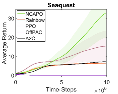
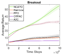
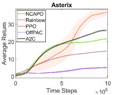
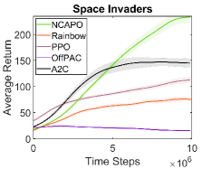
Figure 1: A comparison between the performance of NCAPO and other benchmark methods algorithms in MinAtar. All the results are averaged over 10 random seeds (with the shaded area showing the range of $\text{mean}\pm 0.5\cdot\text{std}$).

Empirical Evaluation. The detailed implementation of NCAPO is provided in Appendix G. From Figure 1, we can observe that NCAPO has the best performance in Seaquest, Breakout, Space Invaders. We also see that NCAPO is more robust across tasks than PPO and Rainbow. For example, Rainbow performs especially well in Asterix, while relatively poorly in Space Invaders. PPO performs relatively strong in Breakout and Seaquest, but converges rather slowly in Asterix. Off-PAC with a uniform behavior policy has very little improvement throughout training in all the tasks due to the issue of fixed behavior policy, which could hardly find sufficiently long trajectories with high scores. By contrast, NCAPO outperforms all the benchmark methods in three out of four environments, while being on par with other methods in the remaining environment.

7 Related Work

Off-Policy Policy Gradients. Off-policy learning via PG has been an on-going research topic. Built on the off-policy PG theorem (Degris et al., 2012; Silver et al., 2014; Zhang et al., 2019; Imani et al., 2018), various off-policy actor-critic algorithms have been developed with an aim to achieve more sample-efficient RL (Wang et al., 2017; Gu et al., 2017a; Chung et al., 2021; Ciosek and Whiteson, 2018; Espeholt et al., 2018; Schmitt et al., 2020). In the standard off-policy PG formulation, the main idea lies in the use of a surrogate objective, which is the expected total return with expectation taken over the stationary distribution induced by the behavior policy. While this design avoids the issue of an exponentially-growing importance sampling ratio, it has been shown that this surrogate objective can suffer from convergence to sub-optimal policies due to distribution mismatch, and distribution correction is therefore needed, either via a learned density correction ratio (Liu et al., 2020b) or emphatic weighting (Maei, 2018; Zhang et al., 2019, 2020). On the other hand, off-policy actor-critic based on NPG has been recently shown to achieve provable sample complexity guarantees in both tabular (Khodadadian et al., 2021b) and linear function approximation setting (Chen and Maguluri, 2022; Chen et al., 2022). Another line of research is on characterizing the convergence of off-policy actor-critic methods in the offline setting, where the learner is given only a fixed dataset of samples (Xu et al., 2021; Huang and Jiang, 2022). Some recent attempts propose to enable off-policy learning beyond the use of policy gradient. For example, (Laroche and Tachet des Combes, 2021) extends the on-policy PG to an off-policy policy update by generalizing the role of the discounted state visitation distribution. (Laroche and Des Combes, 2022) proposes to use the gradient of the cross-entropy loss with respect to the action with maximum Q. Both approaches are shown to attain similar convergence rates as the on-policy true PG. Different from all the above, CAPO serves as the first attempt to address off-policy policy optimization through the lens of coordinate ascent, without using the policy gradient.

Exploiting the Sign of Advantage Function. As pointed out in Section 2, the sign of the advantage function (or temporal difference (TD) residual as a surrogate) can serve as an indicator of policy improvement. For example, (Van Hasselt and Wiering, 2007) proposed Actor Critic Learning Automaton (ACLA), which is designed to reinforce only those state-action pairs with positive TD residual and ignore those pairs with non-positive TD residual. The idea of ACLA is later extended by (Zimmer et al., 2016) to Neural Fitted Actor Critic (NFAC) , which learns neural policies for continuous control, and penalized version of NFAC for improved empirical performance (Zimmer and Weng, 2019). On the other hand, (Tessler et al., 2019) proposes generative actor critic (GAC), a distributional policy optimization approach that leverages the actions with positive advantage to construct a target distribution. By contrast, CAPO takes the first step towards understanding the use of coordinate ascent with convergence guarantees for off-policy RL.

8 Conclusion

We propose CAPO, which takes the first step towards addressing off-policy policy optimization by exploring the use of coordinate ascent in RL. Through CAPO, we enable off-policy learning without the need for importance sampling or distribution correction. We show that the general CAPO can attain asymptotic global convergence and establish the convergence rates of CAPO with several popular coordinate selection rules. Moreover, through experiments, we show that the neural implementation of CAPO can serve as a competitive solution compared to the benchmark RL methods and thereby demonstrates the future potential of CAPO.

Appendix

Appendix A Proofs of the Theoretical Results in Section 3.2

A.1 Proof of Lemma 2

Lemma 3 (Performance Difference Lemma in (Kakade and Langford, 2002)).

For each state $s_{0}$, the difference in the value of $s_{0}$ between two policies $\pi$ and $\pi^{\prime}$ can be characterized as:

$$V^{\pi}\left(s_{0}\right)-V^{\pi^{\prime}}\left(s_{0}\right)=\frac{1}{1-\gamma}\mathbb{E}_{s\sim d_{s_{0}}^{\pi}}\mathbb{E}_{a\sim\pi(\cdot\rvert s)}\left[A^{\pi^{\prime}}(s,a)\right]$$ (20)

Now we are ready to prove Lemma 2. For ease of exposition, we restate Lemma 2 as follows.

Lemma.

Under the CAPO update given by (3.1), we have $V^{\pi_{m+1}}(s)\geq V^{\pi_{m}}(s)$, for all $s\in S$, for all $m\in\mathbb{N}$.

Proof of Lemma 2.

Note that by the definition of $A(s,a)$, we have

$$\sum_{a\in\mathcal{A}}\pi_{m}(a|s)A^{m}(s,a)=0,\quad\forall s\in\mathcal{S}$$ (21)

To simplify notation, let $Z_{m}(s):=\sum_{a\in\mathcal{A}}\exp({\theta_{m}(s,a)})$. Then, $\pi_{m}(a|s)$ and $\pi_{m+1}(a|s)$ can be simplified as:

$$\pi_{m}(a|s)=\frac{\exp({\theta_{m}(s,a)})}{Z_{m}(s)},\quad\pi_{m+1}(a|s)=\frac{\exp({\theta_{m+1}(s,a)})}{Z_{m+1}(s)}.$$ (22)

By Lemma 3, in order to show that $V^{\pi_{m+1}}(s)\geq V^{\pi_{m}}(s),\forall s\in S$, it is sufficient to show that

$$\sum_{a\in\operatorname{\mathcal{A}}}\pi_{m+1}(a|s)A^{m}(s,a)>0,\quad\forall s\in\mathcal{S}.$$ (23)

For ease of notation, we define ${B}_{m}(s):=\{a\rvert(s,a)\in{B}_{m}\}$. To establish (22), we have that for all $s\in\mathcal{S}$,

$$\sum_{a\in\mathcal{A}}\pi_{m+1}(a|s)A^{m}(s,a) =\sum_{a\in\mathcal{A}}\frac{\exp({\theta_{m+1}(s,a)})}{Z_{m+1}(s)}A^{m}(s,a)$$ (24)

$$=\frac{Z_{m}(s)}{Z_{m+1}(s)}\sum_{a\in\mathcal{A}}\frac{\exp({\theta_{m+1}(s,a)})}{Z_{m}(s)}A^{m}(s,a)$$ (25)

$$=\frac{Z_{m}(s)}{Z_{m+1}(s)}\left[\sum_{a\in{B}_{m}(s)}\frac{\exp({\theta_{m+1}(s,a)})}{Z_{m}(s)}A^{m}(s,a)+\sum_{a\not\in{B}_{m}(s)}\frac{\exp({\theta_{m}(s,a)})}{Z_{m}(s)}A^{m}(s,a)\right]$$ (26)

$$>\frac{Z_{m}(s)}{Z_{m+1}(s)}\left[\sum_{a\in{B}_{m}(s)}\frac{\exp({\theta_{m}(s,a)})}{Z_{m}(s)}A^{m}(s,a)+\sum_{a\not\in{B}_{m}(s)}\frac{\exp({\theta_{m}(s,a)})}{Z_{m}(s)}A^{m}(s,a)\right]$$ (27)

$$=\frac{Z_{m}(s)}{Z_{m+1}(s)}\sum_{a\in\mathcal{A}}\pi_{m}(a|s)A^{m}(s,a)$$ (28)

$$=0,$$ (29)

where (27) holds by the CAPO update given by (3.1). ∎

A.2 Proof of Theorem 1

Since $\{V^{m}\}$ is bounded above and enjoys strict improvement by Lemma 2. By the monotone convergence theorem, the limit of $\{V^{m}\}$ is guaranteed to exist. Similarly, we know that the limit of $\{Q^{m}\}$ also exists. We use $V^{(\infty)}(s)$ and $Q^{(\infty)}(s,a)$ to denote the limits of $\{V^{(m)}(s)\}$ and $\{Q^{(m)}(s,a)\}$, respectively. We also define $A^{(\infty)}(s,a):=Q^{(\infty)}(s,a)-V^{(\infty)}(s)$. Our concern is whether the corresponding policy $\pi_{\infty}$ is optimal. Inspired by (Agarwal et al., 2019), we first define the following three sets as

$$I_{0}^{s} :=\left\{a\rvert Q^{(\infty)}(s,a)=V^{(\infty)}(s)\right\},$$ (30)

$$I_{+}^{s} :=\left\{a\rvert Q^{(\infty)}(s,a)>V^{(\infty)}(s)\right\},$$ (31)

$$I_{-}^{s} :=\left\{a\rvert Q^{(\infty)}(s,a)<V^{(\infty)}(s)\right\}.$$ (32)

By definition, $V^{(\infty)}$ is optimal if and only if $I_{+}^{s}$ is empty, for all $s$. We prove by contradiction that $V^{(\infty)}$ is optimal by showing $I_{+}^{s}=\emptyset$.

Main steps of the proof. The proof procedure can be summarized as follows:

• Step 1: We first assume $V^{(\infty)}$ is not optimal so that by definition $\exists s\in\mathcal{S},I_{+}^{s}\neq\emptyset$.

• Step 2: We then show in Lemma 5, $\forall s\in\mathcal{S}$, actions $a_{-}\in I_{-}^{s}$ have zero weights in policy (i.e. $\pi_{\infty}(a_{-}|s)=0$, $\forall a_{-}\in I_{-}^{s}$).

• Step 3: Since the actions in $I_{-}^{s}$ have zero probability, by (21), this directly implies Lemma 6: $\forall I_{+}^{s}\neq\emptyset$, $a\in I_{+}^{s}$ must also have zero probability (i.e. $\pi_{\infty}(a_{+}|s)=0$, $\forall a_{+}\in I_{+}^{s}$).

• Step 4: Moreover, under CAPO, in the sequel we can show 1, which states that as long as 1 is satisfied, there must exist one action $a_{+}\in I_{+}^{s}$ such that $\lim_{m\rightarrow\infty}\pi_{m}(a_{+}|s)=1$. This contradicts the assumption that $\exists s\in\mathcal{S},I_{+}^{s}\neq\emptyset$, proving that $I_{+}^{s}=\emptyset,\forall s\in\mathcal{S}$.

Lemma 4.

Under CAPO, there exists $M_{1}$ such that for all $m>M_{1},s\in\mathcal{S},a\in\mathcal{A}$, we have :

$$A^{(m)}(s,a)<-\frac{\Delta}{4}, \quad\text{ for }a\in I_{-}^{s},$$ (33)

$$A^{(m)}(s,a)>\frac{\Delta}{4}, \quad\text{ for }a\in I_{+}^{s},$$ (34)

where $\Delta:=\min_{\left\{s,a\rvert A^{(\infty)}(s,a)\neq 0\right\}}\left|A^{(\infty)}(s,a)\right|$.

Proof of Lemma 4.

Given the strict policy improvement property of CAPO in Lemma 2, this can be shown by applying Lemma C.4 in (Agarwal et al., 2019). ∎

Lemma 5.

Under CAPO, $\pi_{\infty}(a_{-}|s)=0,\forall s\in\mathcal{S},a_{-}\in I^{s}_{-}$.

Proof of Lemma 5.

Lemma 4 shows that for all $m>M_{1}$, the sign of $A^{(m)}(s,a)$ is fixed. Moreover, we know that under CAPO update, $\theta_{m}(s,a_{-})$ is non-increasing, $\forall a_{-}\in I^{s}_{-},\forall m>M_{1}$. Similarly, $\forall a_{+}\in I^{s}_{+},m>M_{1}$, $\theta_{m}(s,a_{+})$ is non-decreasing. By 1, all the state-action pairs with negative advantage are guaranteed to be sampled for infinitely many times as $m\rightarrow\infty$. Under the CAPO update in (3.1), we have

$$\theta_{m+1}(s,a_{-})-\theta_{m}(a_{-}\rvert s)\leq-\log(\frac{1}{\pi_{m}(a_{-}\rvert s)})<0.$$ (35)

Given the infinite visitation, we know that $\lim_{m\rightarrow\infty}\theta_{m}(s,a_{-})=-\infty$. ∎

We now show in Lemma 6 that Lemma 5 implies $\sum_{a_{+}\in I_{+}^{s}}\pi_{\infty}(a_{+}\rvert s)=0$.

Lemma 6.

If $I_{+}^{s}\neq\emptyset$ is true, then Lemma 5 implies $\sum_{a_{+}\in I_{+}^{s}}\pi_{\infty}(a_{+}|s)=0$.

Proof of Lemma 6.

Recall from (21) that $\sum_{a\in\mathcal{A}}\pi_{m}(a\rvert s)A^{m}(s,a)=0,\forall s\in\mathcal{S},m>0$. By definition, $\sum_{a_{0}\in I_{0}^{s}}\pi_{\infty}(a_{0}|s)A^{\infty}(s,a_{0})=0$, which directly implies that

$$\sum_{a_{+}\in I_{+}^{s}}\pi_{\infty}(a_{+}|s)A^{\infty}(s,a_{+}) =\sum_{a\in\mathcal{A}}\pi_{\infty}(a\rvert s)A^{\infty}(s,a)-\sum_{a_{0}\in I_{0}^{s}}\pi_{\infty}(a_{0}\rvert s)A^{\infty}(s,a)-\sum_{a_{-}\in I_{-}^{s}}\pi_{\infty}(a_{-}\rvert s)A^{\infty}(s,a)$$ (36)

$$=0-0-0=0,$$ (37)

where the second equality holds by Lemma 5. Since $A^{\infty}(s,a_{+})>0$ and $\pi_{\infty}(a_{+}\rvert s)\geq 0$, we have $\sum_{a_{+}\in I_{+}^{s}}\pi_{\infty}(a_{+}\rvert s)=0$. This completes the proof of Lemma 6. ∎

In Lemma 6, we have that if $I_{+}^{s}\neq\emptyset$ is true, then $\pi_{m}(a_{+}\rvert s)\rightarrow 0$ as $m\rightarrow\infty$. To establish contradiction, we proceed to show in the following 1 that there must exist one action $a\in I_{+}^{s}$ such that $\lim_{m\rightarrow\infty}\pi_{m}(a|s)=1$, which contradicts Lemma 6 and hence implies the desired result that $I_{+}^{s}=\emptyset$.

If $I_{+}^{s}\neq\emptyset$ is true, then there exist $K$ such that $\forall m>K,s\in\mathcal{S}$, we have:

$$Q^{m}(s,a^{+})>Q^{m}(s,a^{0})>Q^{m}(s,a^{-}),\quad\text{for all $a^{+}\in I^{s}_{+}$, $a^{0}\in I^{s}_{0}$, $a^{-}\in I^{s}_{-}$}.$$ (38)

Without loss of generality, assume that the order of $Q^{m}$, $\forall m>K$, can be written as

$$Q^{m}(s,\tilde{a}^{+})>Q^{m}(s,a_{1})>Q^{m}(s,a_{2})>\dots>Q^{m}(s,a_{|\mathcal{A}|-1}),\quad\text{provided that $I_{+}^{s}\neq\emptyset$},$$ (39)

where $\tilde{a}^{+}:=\operatorname*{argmax}_{a^{+}\in I^{s}_{+}}Q^{(\infty)}(s,a^{+})$. Note that we simplify the case above by considering "strictly greater than" instead of "greater than or equal to", but the simplification can be relaxed with a little extra work.

Claim 1.

If $I_{+}^{s}\neq\emptyset$ is true, then there must exist one action $a_{+}\in I_{+}^{s}$ such that $\lim_{m\rightarrow\infty}\pi_{m}(a_{+}|s)=1$ under (3.1) with $\alpha_{m}(s,a)\geq\log\frac{1}{\pi_{m}(a|s)}$.

To establish 1, we show that if $I_{+}^{s}\neq\emptyset$, then $\lim_{m\rightarrow\infty}\pi_{m}(a|s)=0$ for all $a\neq\tilde{a}^{+}$ by induction. For ease of exposition, we first present the following propositions.

Proposition 1.

For any $m\geq 1,s\in\mathcal{S},a\in\mathcal{A}$, if $A^{m}(s,a)\leq 0$ and $\exists\enspace a^{\prime}\neq a$, $a^{\prime}\in{B}_{m}(s)$, satisfying $A^{m}(s,a^{\prime})>0$, then $\pi_{m+1}(a|s)\leq\frac{1}{2}$, regardless of whether $a\in{B}_{m}(s)$ or not.

Proof of 1.

Since $A^{m}(s,a)\leq 0$, we have $\operatorname{sign}(A^{m}(s,a))\cdot\alpha_{m}(s,a)\leq 0$. As a result, we have:

$$\begin{cases}\pi_{m+1}(a|s)=\frac{\exp({\theta_{m}(s,a)+\operatorname{sign}(A^{m}(s,a))\cdot\alpha_{m}(s,a)})}{Z_{m+1}(s)}\leq\frac{\exp({\theta_{m}(s,a)})}{Z_{m+1}(s)}\leq\frac{Z_{m}(s)}{Z_{m+1}(s)}\\ \pi_{m+1}(a^{{}^{\prime}}|s)=\frac{\exp({\theta_{m}(s,a^{\prime})+\alpha_{m}(s,a^{\prime})})}{Z_{m+1}(s)}\geq\frac{\exp({\theta_{m}(s,a^{\prime})+\log(\frac{1}{\pi_{m}(a^{\prime}|s)})})}{Z_{m+1}(s)}=\frac{Z_{m}(s)}{Z_{m+1}(s)}\end{cases}$$ (40)

Hence, we have $\pi_{m+1}(a^{{}^{\prime}}|s)\geq\pi_{m+1}(a|s)$. Since $\pi_{m+1}(a^{{}^{\prime}}|s)+\pi_{m+1}(a|s)\leq 1$, we get $\pi_{m+1}(a|s)\leq\frac{1}{2}$.

∎

Proposition 2.

For any $s\in\mathcal{S},a\in\mathcal{A}\setminus\left\{\tilde{a}^{+}\right\}$, if $\exists\enspace T\in\mathbb{N}$ such that $\forall m>T$, $A^{m}(s,a)\leq 0$, then $\exists\enspace n\in\mathbb{N}$, $\bar{K}\in\mathbb{N}$ such that $A^{m+n+1}(s,a)<0\text{, }\forall\enspace m>\bar{K}$.

Proof of 2.

By Condition 1 and $I_{+}^{s}\neq\emptyset$, there exist some finite $n\in\mathbb{N}$ such that $\exists\enspace a^{\prime}\neq a$, $a^{\prime}\in{B}_{m+n}(s)$, satisfying $A^{m+n+1}(s,a^{\prime})>0$. Then, by 1, we have

$$\pi_{m+n+1}(a|s)\leq\frac{1}{2},\quad\text{$\forall m\geq T$}.$$ (41)

Hence, we have

$$V^{m+n+1}(s)=\sum_{a\in\mathcal{A}}\pi_{m+n+1}(a|s)\cdot Q^{m+n+1}(s,a)\geq\frac{1}{2}\cdot\left(Q^{m+n+1}(s,a)+Q^{m+n+1}(s,a^{\prime})\right)$$ (42)

where $$a^{\prime}=\underset{\begin{subarray}{c}a^{\prime\prime}\in\mathcal{A}\\ Q^{\infty}(s,a^{\prime\prime})>Q^{\infty}(s,a)\end{subarray}}{\mathrm{argmin}}Q^{\infty}(s,a^{\prime\prime})$$ (43)

Moreover, by the ordering of $Q^{m}$ and that $\lim_{m\rightarrow\infty}Q^{m}(s,a)=Q^{\infty}(s,a)$, for $\epsilon=\frac{1}{4}\cdot\left(Q^{\infty}(s,a^{\prime})-Q^{\infty}(s,a)\right)>0$, $\exists\enspace\bar{T}$ such that for all $m>\bar{T}$:

$$\begin{cases}Q^{m}(s,a)\in\left(Q^{\infty}(s,a)-\epsilon,Q^{\infty}(s,a)+\epsilon\right)\\ Q^{m}(s,a^{\prime})\in\left(Q^{\infty}(s,a^{\prime})-\epsilon,Q^{\infty}(s,a^{\prime})+\epsilon\right)\end{cases}$$ (44)

Finally, we have that for all $m>\max\left\{T,\bar{T}\right\}$:

$$V^{m+n+1}(s) \geq\frac{1}{2}\cdot\left(Q^{m+n+1}(s,a)+Q^{m+n+1}(s,a^{\prime})\right)$$ (45)

$$>\frac{1}{2}\cdot\left((Q^{\infty}(s,a))+(Q^{\infty}(s,a^{\prime}))\right)$$ (46)

$$>\frac{1}{2}\cdot\left(Q^{\infty}(s,a)+Q^{\infty}(s,a^{\prime})\right)-\epsilon$$ (47)

$$=Q^{\infty}(s,a)+\epsilon>Q^{m+n+1}(s,a).$$ (48)

The above is equivalent to $A^{m+n+1}(s,a)<0\enspace\forall\enspace m>\bar{K}$, where $\bar{K}=\max\left\{T,\bar{T}\right\}$. ∎

Proposition 3.

If $V^{m}(s)\in\left(Q^{m}(s,a_{|\mathcal{A}|-k}),Q^{m}(s,a_{|\mathcal{A}|-(k+2)})\right)$, then $\exists\enspace T^{\prime}\in\mathbb{N}$ such that for all $m>T^{\prime}$:

$$\frac{\sum_{\begin{subarray}{c}a\in\mathcal{A}\\ Q^{\infty}(s,a)>Q^{\infty}(s,a_{|\mathcal{A}|-(k+1)})\end{subarray}}\pi_{m}(a|s)}{\sum_{\begin{subarray}{c}a\in\mathcal{A}\\ Q^{\infty}(s,a)<Q^{\infty}(s,a_{|\mathcal{A}|-(k+1)})\end{subarray}}\pi_{m}(a|s)}\geq\frac{Q^{m}(s,a_{|\mathcal{A}|-(k+1)})-Q^{m}(s,a_{|\mathcal{A}|-1})}{Q^{m}(s,a_{|\mathcal{A}|-(k+2)})-Q^{m}(s,a_{|\mathcal{A}|-(k+1)})}$$ (49)

provided $$V^{m}(s)\in\left(Q^{m}(s,a_{|\mathcal{A}|-k}),Q^{m}(s,a_{|\mathcal{A}|-(k+2)})\right)$$ (50)

Proof of 3.

Since $V^{m}(s)\in\left(Q^{m}(s,a_{|\mathcal{A}|-k}),Q^{m}(s,a_{|\mathcal{A}|-(k+2)})\right)$, we have $A^{m}(s,a_{|\mathcal{A}|-j})<0,\enspace\forall\enspace j=1,2,\dots,k$. By Condition 1, there exists some finite $n\in\mathbb{N}$ such that $\bar{a}^{+}\in\mathcal{B}_{m+n}(s)$ for some $\bar{a}^{+}\in\left\{\tilde{a}^{+},a_{1},a_{2},\dots,a_{|\mathcal{A}|-(k+2)}\right\}$.
Hence, we have that for all $\bar{a}^{-}\in\left\{a_{|\mathcal{A}|-k},a_{|\mathcal{A}|-(k-1)},\dots,a_{|\mathcal{A}|-1}\right\}$,

$$\frac{\pi_{m+n+1}(\bar{a}^{+}|s)}{\pi_{m+n+1}(\bar{a}^{-}|s)}\geq\frac{\frac{e^{\theta_{m+n}(s,\bar{a}^{+})+\log{\frac{1}{\pi_{m+n}(\bar{a}^{+}|s)}}}}{Z_{m+n+1}(s)}}{\frac{e^{\theta_{m+n}(s,\bar{a}^{-})}}{Z_{m+n+1}(s)}}=\frac{Z_{m+n}(s)}{e^{\theta_{m+n}(s,\bar{a}^{-})}}=\frac{1}{\pi_{m+n}(\bar{a}^{-}|s)}.$$ (51)

Since $\lim_{m\rightarrow\infty}\pi_{m}(s,a)=0$, we have $\forall z\in\mathbb{Z}$, $\exists\enspace T\in\mathbb{N}$ such that $\frac{\pi_{m+n+1}(\bar{a}^{+}|s)}{\pi_{m+n+1}(\bar{a}^{-}|s)}\geq z,\enspace\forall m>T$. For $m>K$, we have $Q^{m}(s,a_{|\mathcal{A}|-(k+2)})-Q^{m}(s,a_{|\mathcal{A}|-(k+1)})>0$. Hence, by simply choosing $z=\frac{1}{\mathcal{A}}\cdot\frac{Q^{m}(s,a_{|\mathcal{A}|-(k+1)})-Q^{m}(s,a_{|\mathcal{A}|-1})}{Q^{m}(s,a_{|\mathcal{A}|-(k+2)})-Q^{m}(s,a_{|\mathcal{A}|-(k+1)})}$ and taking the summation of the ratio over $\bar{a}^{+}$ and $\bar{a}^{-}$, we can reach the desired result with $T^{\prime}=\max\left\{K,T\right\}$. ∎

Now, we are ready to prove 1 by an induction argument.

Proof of 1.

• Show that if $I_{+}^{s}\neq\emptyset$, then $\lim_{m\rightarrow\infty}\pi_{m}(a_{|\mathcal{A}|-1}|s)=0$:
  By the ordering of $Q^{m}$, we have:

  $$V^{m}(s)=\sum_{a\in\mathcal{A}}\pi_{m}(a|s)\cdot Q^{m}(s,a)\geq 1\cdot Q^{m}(s,a_{|\mathcal{A}|-1})\text{, \quad$\forall m>K$ }.$$ (52)

  Hence, for all $m>K$, we have:

  $$A^{m}(s,a_{|\mathcal{A}|-1})=Q^{m}(s,a_{|\mathcal{A}|-1})-V^{m}(s)\leq Q^{m}(s,a_{|\mathcal{A}|-1})-Q^{m}(s,a_{|\mathcal{A}|-1})=0.$$ (53)

  Therefore, by 2, we have $\exists\enspace n_{|\mathcal{A}|-1}\in\mathbb{N}$, $K_{|\mathcal{A}|-1}\in\mathbb{N}$ such that:

  $$A^{m+n_{|\mathcal{A}|-1}+1}(s,a_{|\mathcal{A}|-1})<0\text{, \quad$\forall m>K_{|\mathcal{A}|-1}$ }.$$ (54)

  Moreover,

  $$\operatorname{sign}(A^{m}(s,a_{|\mathcal{A}|-1}))\cdot\alpha_{m}\left(s,a_{|\mathcal{A}|-1}\right)<0\text{, \quad$\forall m>K_{|\mathcal{A}|-1}$. }$$ (55)

  With the monotone-decreasing property and the infinite visitation condition, it is guaranteed that $\lim_{m\rightarrow\infty}\theta_{m}(s,a_{|\mathcal{A}|-1})=-\infty$. Hence, we have $\lim_{m\rightarrow\infty}\pi_{m}(s,a_{|\mathcal{A}|-1})=0$.

• Suppose that $\lim_{m\rightarrow\infty}\pi_{m}(a_{|\mathcal{A}|-1}|s)=\lim_{m\rightarrow\infty}\pi_{m}(a_{|\mathcal{A}|-2}|s)=\dots=\lim_{m\rightarrow\infty}\pi_{m}(a_{|\mathcal{A}|-k}|s)=0$, where $k\in\left[1,(|\mathcal{A}|-2)\right]$. Then we would like to derive $\lim_{m\rightarrow\infty}\pi_{m}(a_{|\mathcal{A}|-(k+1)}|s)$:
  By the above assumption, we have:

  $$\lim_{m\rightarrow\infty}\sum_{\begin{subarray}{c}a\in\mathcal{A}\\ Q^{\infty}(s,a)<Q^{\infty}(s,a_{|\mathcal{A}|-(k+1)})\end{subarray}}\pi_{m}(a|s)=0$$ (56)

  By 3, $\exists\enspace K^{\prime}_{|\mathcal{A}|-(k+1)}\in\mathbb{N}$ such that $\forall\enspace m>K^{\prime}_{|\mathcal{A}|-(k+1)}$, we can establish the ratio between the summation of policy weight of the policy worse than $a_{|\mathcal{A}|-(k+1)}$ and the policy better than $a_{|\mathcal{A}|-(k+1)}$:

  $$\frac{\sum_{\begin{subarray}{c}a\in\mathcal{A}\\ Q^{\infty}(s,a)>Q^{\infty}(s,a_{|\mathcal{A}|-(k+1)})\end{subarray}}\pi_{m}(a|s)}{\sum_{\begin{subarray}{c}a\in\mathcal{A}\\ Q^{\infty}(s,a)<Q^{\infty}(s,a_{|\mathcal{A}|-(k+1)})\end{subarray}}\pi_{m}(a|s)}\geq\frac{Q^{m}(s,a_{|\mathcal{A}|-(k+1)})-Q^{m}(s,a_{|\mathcal{A}|-1})}{Q^{m}(s,a_{|\mathcal{A}|-(k+2)})-Q^{m}(s,a_{|\mathcal{A}|-(k+1)})}$$ (57)

  provided $$V^{m}(s)\in\left(Q^{m}(s,a_{|\mathcal{A}|-k}),Q^{m}(s,a_{|\mathcal{A}|-(k+2)})\right)$$ (58)

  And by the ordering of $Q^{m}$, we have:

  $$V^{m}(s) =\sum_{a\in\mathcal{A}}\pi_{m}(a|s)\cdot Q^{m}(s,a)$$ (59)

  $$=\left[\sum_{\begin{subarray}{c}a\in\mathcal{A}\\ Q^{\infty}(s,a)>Q^{\infty}(s,a_{|\mathcal{A}|-(k+1)})\end{subarray}}\pi_{m}(a|s)\cdot Q^{m}(s,a)+Q^{m}(s,a_{|\mathcal{A}|-(k+1)})\cdot\pi_{m}(a_{|\mathcal{A}|-(k+1)}|s)\right.$$ (60)

  $$\left.\quad+\sum_{\begin{subarray}{c}a\in\mathcal{A}\\ Q^{\infty}(s,a)<Q^{\infty}(s,a_{|\mathcal{A}|-(k+1)})\end{subarray}}\pi_{m}(a|s)\cdot Q^{m}(s,a)\right]$$ (61)

  $$\geq\left[Q^{m}(s,a_{|\mathcal{A}|-(k+2)})\cdot\sum_{\begin{subarray}{c}a\in\mathcal{A}\\ Q^{\infty}(s,a)>Q^{\infty}(s,a_{|\mathcal{A}|-(k+1)})\end{subarray}}\pi_{m}(a|s)+Q^{m}(s,a_{|\mathcal{A}|-(k+1)})\cdot\pi_{m}(a_{|\mathcal{A}|-(k+1)}|s)\right.$$ (62)

  $$\left.\quad+Q^{m}(s,a_{|\mathcal{A}|-1})\cdot\sum_{\begin{subarray}{c}a\in\mathcal{A}\\ Q^{\infty}(s,a)<Q^{\infty}(s,a_{|\mathcal{A}|-(k+1)})\end{subarray}}\pi_{m}(a|s)\right]\text{, \quad$\forall m>K$ }.$$ (63)

  Hence, for all $m>K^{\prime}_{|\mathcal{A}|-(k+1)}$, we have:

  $$A^{m}(s,a_{|\mathcal{A}|-(k+1)}) =Q^{m}(s,a_{|\mathcal{A}|-(k+1)})-V^{m}(s)$$ (64)

  $$\leq Q^{m}(s,a_{|\mathcal{A}|-(k+1)})-\left[Q^{m}(s,a_{|\mathcal{A}|-(k+2)})\cdot\sum_{\begin{subarray}{c}a\in\mathcal{A}\\ Q^{\infty}(s,a)>Q^{\infty}(s,a_{|\mathcal{A}|-(k+1)})\end{subarray}}\pi_{m}(a|s)\right.$$ (65)

  $$\left.\qquad\qquad\qquad\qquad\qquad\quad+Q^{m}(s,a_{|\mathcal{A}|-(k+1)})\cdot\pi_{m}(a_{|\mathcal{A}|-(k+1)}|s)\right.$$ (66)

  $$\left.\qquad\qquad\qquad\qquad\qquad\quad+Q^{m}(s,a_{|\mathcal{A}|-1})\cdot\sum_{\begin{subarray}{c}a\in\mathcal{A}\\ Q^{\infty}(s,a)<Q^{\infty}(s,a_{|\mathcal{A}|-(k+1)})\end{subarray}}\pi_{m}(a|s)\right]$$ (67)

  $$=\left(Q^{m}(s,a_{|\mathcal{A}|-(k+1)})-Q^{m}(s,a_{|\mathcal{A}|-(k+2)})\right)\cdot\sum_{\begin{subarray}{c}a\in\mathcal{A}\\ Q^{\infty}(s,a)>Q^{\infty}(s,a_{|\mathcal{A}|-(k+1)})\end{subarray}}\pi_{m}(a|s)$$ (69)

  $$\quad+\left(Q^{m}(s,a_{|\mathcal{A}|-(k+1)})-Q^{m}(s,a_{|\mathcal{A}|-1})\right)\cdot\sum_{\begin{subarray}{c}a\in\mathcal{A}\\ Q^{\infty}(s,a)<Q^{\infty}(s,a_{|\mathcal{A}|-(k+1)})\end{subarray}}\pi_{m}(a|s)$$ (70)

  $$\leq\left(Q^{m}(s,a_{|\mathcal{A}|-(k+1)})-Q^{m}(s,a_{|\mathcal{A}|-(k+2)})\right)\cdot\sum_{\begin{subarray}{c}a\in\mathcal{A}\\ Q^{\infty}(s,a)>Q^{\infty}(s,a_{|\mathcal{A}|-(k+1)})\end{subarray}}\pi_{m}(a|s)$$ (71)

  $$\quad+\left(Q^{m}(s,a_{|\mathcal{A}|-(k+1)})-Q^{m}(s,a_{|\mathcal{A}|-1})\right)\cdot\frac{Q^{m}(s,a_{|\mathcal{A}|-(k+2)})-Q^{m}(s,a_{|\mathcal{A}|-(k+1)})}{Q^{m}(s,a_{|\mathcal{A}|-(k+1)})-Q^{m}(s,a_{|\mathcal{A}|-1})}$$ (72)

  $$\qquad\cdot\sum_{\begin{subarray}{c}a\in\mathcal{A}\\ Q^{\infty}(s,a)>Q^{\infty}(s,a_{|\mathcal{A}|-(k+1)})\end{subarray}}\pi_{m}(a|s)$$ (73)

  $$=0$$ (74)

  By 2, we have $\exists\enspace n_{|\mathcal{A}|-(k+1)}\in\mathbb{N}$, $K_{|\mathcal{A}|-(k+1)}\in\mathbb{N}$ such that:

  $$A^{m+n_{|\mathcal{A}|-(k+1)}+1}(s,a_{|\mathcal{A}|-(k+1)})<0\text{, \quad$\forall m>K_{|\mathcal{A}|-(k+1)}$ }$$ (75)

  Moreover,

  $$\operatorname{sign}(A^{m}(s,a_{|\mathcal{A}|-1}))\cdot\alpha_{m}\left(s,a_{|\mathcal{A}|-(k+1)}\right)<0\text{, \quad$\forall m>K_{|\mathcal{A}|-(k+1)}$ }$$ (76)

  With the monotone-decreasing property and the infinite visitation, it is guaranteed that $\lim_{m\rightarrow\infty}\theta_{m}(s,a_{|\mathcal{A}|-(k+1)})=-\infty$. Hence we have $\lim_{m\rightarrow\infty}\pi_{m}(s,a_{|\mathcal{A}|-(k+1)})=0$.
  

  Finally we complete the induction and so we conclude that $\forall a\neq\tilde{a^{+}}$, $\lim_{m\rightarrow\infty}\pi_{m}(s,a)=0$, which is equivalent to $\lim_{m\rightarrow\infty}\pi_{m}(s,\tilde{a^{+}})=1$. This completes the proof of 1.

∎

Now we are ready to put everything together and prove Theorem 1. For ease of exposition, we restate Theorem 1 as follows.

Theorem.

Consider a tabular softmax parameterized policy $\pi_{\theta}$, under (3.1) with ${\alpha_{m}(s,a)\geq\log(\frac{1}{\pi_{\theta_{m}}(a\rvert s)})}$, if Condition 1 is satisfied, then we have $V^{\pi_{m}}(s)\rightarrow V^{*}(s)$ as $m\rightarrow\infty$, for all $s\in\mathcal{S}$.

Proof of Theorem 1.

In 1, we have that if $I_{+}^{s}\neq\emptyset$ is true, then there must exist one action $a\in I_{+}^{s}$ such that $\lim_{m\rightarrow\infty}\pi_{m}(a|s)=1$. This leads to the contradiction with Lemma 6, and finally we get the desired result that $I_{+}^{s}=\emptyset$, implying that $V^{(\infty)}$ is optimal. ∎

Appendix B Proofs of the Convergence Rates of CAPO in Section 3.3

Lemma 7.

$|A^{m}(s,a)|\leq\frac{1}{1-\gamma}\cdot(1-\pi_{m}(a|s))$,  for all $(s,a)\in\mathcal{S}\times\mathcal{A}$.

Proof of Lemma 7.

If $A^{m}(s,a)>0$ :

$$|A^{m}(s,a)| =Q^{\pi_{m}}(s,a)-V^{\pi_{m}}(s)$$ (77)

$$=Q^{\pi_{m}}(s,a)-\sum_{a^{\prime}\in\mathcal{A}}\pi_{m}(a^{\prime}|s)\cdot Q^{\pi_{m}}(s,a^{\prime})$$ (78)

$$\leq Q^{\pi_{m}}(s,a)-\pi_{m}(a|s)\cdot Q^{\pi_{m}}(s,a)$$ (79)

$$=Q^{\pi_{m}}(s,a)\cdot(1-\pi_{m}(a|s))$$ (80)

$$\leq\frac{1}{1-\gamma}\cdot(1-\pi_{m}(a|s))$$ (81)

If $A^{m}(s,a)\leq 0$ :

$$|A^{m}(s,a)| =V^{\pi_{m}}(s)-Q^{\pi_{m}}(s,a)$$ (82)

$$=\sum_{a^{\prime}\in\mathcal{A}}\pi_{m}(a^{\prime}|s)\cdot Q^{\pi_{m}}(s,a^{\prime})-Q^{\pi_{m}}(s,a)$$ (83)

$$=\sum_{a^{\prime}\neq a}\pi_{m}(a^{\prime}|s)\cdot Q^{\pi_{m}}(s,a^{\prime})-(1-\pi_{m}(a|s))\cdot Q^{\pi_{m}}(s,a)$$ (84)

$$\leq\sum_{a^{\prime}\neq a}\pi_{m}(a^{\prime}|s)\cdot Q^{\pi_{m}}(s,a^{\prime})$$ (85)

$$\leq\frac{1}{1-\gamma}\cdot\sum_{a^{\prime}\neq a}\pi_{m}(a^{\prime}|s)$$ (86)

$$=\frac{1}{1-\gamma}\cdot(1-\pi_{m}(a|s))$$ (87)

∎

Lemma 8.

$\left(V^{*}(s)-V^{\pi_{m}}(s)\right)^{2}\leq\left(\frac{1}{1-\gamma}\cdot A^{m}(\tilde{s_{m}},\tilde{a_{m}})\right)^{2}$, for all $m\geq 1$ where $(\tilde{s_{m}},\tilde{a_{m}})=\underset{(s,a)\in\mathcal{S}\times\mathcal{A}}{\operatorname*{argmax}}A^{m}(s,a)$.

Proof of Lemma 8.

$$\left(V^{*}(s)-V^{\pi_{m}}(s)\right)^{2} =\left(\frac{1}{1-\gamma}\cdot\sum_{s^{\prime}\in\mathcal{S}}d^{\pi^{*}}_{s}(s^{\prime})\sum_{a^{\prime}\in\mathcal{A}}\pi^{*}(a^{\prime}|s^{\prime})\cdot A^{m}(s^{\prime},a^{\prime})\right)^{2}$$ (88)

$$\leq\left(\frac{1}{1-\gamma}\cdot\sum_{s^{\prime}\in\mathcal{S}}d^{\pi^{*}}_{s}(s^{\prime})\cdot\underset{a^{\prime}\in\mathcal{A}}{\max}A^{m}(s^{\prime},a^{\prime})\right)^{2}$$ (89)

$$\leq\left(\frac{1}{1-\gamma}\cdot\underset{(s^{\prime},a^{\prime})\in\mathcal{S}\times\mathcal{A}}{\max}A^{m}(s^{\prime},a^{\prime})\right)^{2}$$ (90)

$$=\left(\frac{1}{1-\gamma}\cdot A^{m}(\tilde{s_{m}},\tilde{a_{m}})\right)^{2}$$ (91)

The first equation holds by Lemma 3.
The first and the second inequality hold since the value inside the quadratic term is non-negative.

∎

Lemma 9.

$V^{*}(\rho)-V^{\pi_{m}}(\rho)\leq\frac{1}{1-\gamma}\cdot\left\|\frac{1}{\mu}\right\|_{\infty}\cdot\left(V^{*}(\mu)-V^{\pi_{m}}(\mu)\right)$

Proof of Lemma 9.

$$V^{*}(\rho)-V^{\pi_{m}}(\rho) =\frac{1}{1-\gamma}\cdot\sum_{s\in\mathcal{S}}d^{\pi^{*}}_{\rho}(s)\sum_{a\in\mathcal{A}}\pi^{*}(a|s)\cdot A^{m}(s,a)$$ (92)

$$=\frac{1}{1-\gamma}\cdot\sum_{s\in\mathcal{S}}d^{\pi^{*}}_{\mu}(s)\cdot\frac{d^{\pi^{*}}_{\rho}(s)}{d^{\pi^{*}}_{\mu}(s)}\sum_{a^{\prime}\in\mathcal{A}}\pi^{*}(a|s)\cdot A^{m}(s,a)$$ (93)

$$\leq\frac{1}{1-\gamma}\cdot\left\|\frac{1}{d^{\pi^{*}}_{\mu}}\right\|_{\infty}\cdot\sum_{s\in\mathcal{S}}d^{\pi^{*}}_{\mu}(s)\sum_{a^{\prime}\in\mathcal{A}}\pi^{*}(a|s)\cdot A^{m}(s,a)$$ (94)

$$\leq\frac{1}{(1-\gamma)^{2}}\cdot\left\|\frac{1}{\mu}\right\|_{\infty}\cdot\sum_{s\in\mathcal{S}}d^{\pi^{*}}_{\mu}(s)\sum_{a^{\prime}\in\mathcal{A}}\pi^{*}(a|s)\cdot A^{m}(s,a)$$ (95)

$$=\frac{1}{1-\gamma}\cdot\left\|\frac{1}{\mu}\right\|_{\infty}\cdot\left(V^{*}(\mu)-V^{\pi_{m}}(\mu)\right)$$ (96)

The first and the last equation holds by the performance difference lemma in Lemma 3.
The first and second inequality holds since the value inside the summation is non-negative.

∎

Lemma 10.

$d^{\pi}_{\mu}(s)\geq(1-\gamma)\cdot\mu(s)$,  for any $\pi,s\in\mathcal{S}$ where $\mu(s)$ is some starting state distribution of the MDP.

Proof of Lemma 10.

$$d^{\pi}_{\mu}(s) =\underset{s_{0}\sim\mu}{\mathbb{E}}\left[d^{\pi}_{\mu}(s)\right]$$ (97)

$$=\underset{s_{0}\sim\mu}{\mathbb{E}}\left[(1-\gamma)\cdot\sum_{t=0}^{\infty}\gamma^{t}\cdot\mathbb{P}(s_{t}=s\>|\>s_{0},\pi)\right]$$ (98)

$$\geq\underset{s_{0}\sim\mu}{\mathbb{E}}\left[(1-\gamma)\cdot\mathbb{P}(s_{0}=s\>|\>s_{0},\pi)\right]$$ (99)

$$=(1-\gamma)\cdot\mu(s)$$ (100)

The first equation holds by the performance difference lemma in Lemma 3.
The second and the third equation hold since the value inside quadratic term is non-negative.

∎

Lemma 11.

Given $\delta_{m+1}\leq\delta_{m}-c\cdot\delta_{m}^{2}$ where $\delta_{m}\leq\frac{1}{1-\gamma}$ for all $m\geq 1$ and $c\leq\frac{1-\gamma}{2}$, then $\delta_{m}\leq\frac{1}{c}\cdot\frac{1}{m}$ and $\sum_{m=1}^{M}\delta_{m}\leq\min{\left\{\sqrt{\frac{M}{c\cdot(1-\gamma)}},\frac{\log M+1}{c}\right\}}$ for all $m\geq 1$.

Proof of Lemma 11.

We prove this lemma by induction. For $m\leq 2$, $\delta_{m}\leq\frac{1}{c}\cdot\frac{1}{m}$ directly holds since $c\leq\frac{1-\gamma}{2}$ and $\delta_{m}\leq\frac{1}{1-\gamma}$.
Let $f_{t}(x)=x-c\cdot x^{2}=-c(x-\frac{1}{2c})^{2}+\frac{1}{4c}$. Then $f_{t}(x)$ is monotonically increasing in $[0,\frac{1}{2c}]$. And so we have :

$$\delta_{m+1} \leq f_{t}(\delta_{m})$$ (101)

$$\leq f_{t}(\frac{1}{c}\cdot\frac{1}{m})$$ (102)

$$=\frac{1}{c}\cdot(\frac{1}{m}-\frac{1}{m^{2}})$$ (103)

$$\leq\frac{1}{c}\cdot\frac{1}{m+1}$$ (104)

and by summing up $\delta_{m}$, we have :

$$\sum_{m=1}^{M}\delta_{m} \leq\sum_{m=1}^{M}\frac{1}{c}\cdot\frac{1}{m}$$ (105)

$$=\frac{1}{c}\cdot\sum_{m=1}^{M}\frac{1}{m}$$ (106)

$$\leq\frac{1}{c}\cdot(\ln{M}+1)$$ (107)

On the other hand, we also have :

$$\sum_{m=1}^{M}\delta_{m}^{2} \leq\frac{1}{c}\cdot\sum_{m=1}^{M}(\delta_{m}-\delta_{m+1})$$ (108)

$$\leq\frac{1}{c}\cdot(\delta_{1}-\delta_{M+1})$$ (109)

$$\leq\frac{1}{c}\cdot\frac{1}{1-\gamma}$$ (110)

Therefore, by Cauchy-Schwarz,

$$\sum_{m=1}^{M}\delta_{m} \leq\sqrt{M}\cdot\sqrt{\sum_{m=1}^{M}\delta_{m}^{2}}$$ (111)

$$\leq\sqrt{M}\cdot\sqrt{\frac{1}{c}\cdot\frac{1}{1-\gamma}}$$ (112)

$$=\sqrt{\frac{M}{c\cdot(1-\gamma)}}$$ (113)

∎

Lemma 12.

Under the CAPO update (3.1) with ${\alpha_{m}(s,a)=\log(\frac{1}{\pi_{\theta_{m}}(a\rvert s)})}$, if $B_{m}=\left\{(s_{m},a_{m})\right\}$ and $A^{m}(s_{m},a_{m})>0$, then the policy weight difference $\pi_{m+1}(a|s)-\pi_{m}(a|s)$ can be written as :

$$\pi_{m+1}(a|s)-\pi_{m}(a|s)=\begin{cases}\frac{(1-\pi_{m}(a_{m}|s_{m}))^{2}}{2-\pi_{m}(a_{m}|s_{m})}&\text{, if }s=s_{m},a=a_{m}\\ -\frac{1-\pi_{m}(a_{m}|s_{m})}{2-\pi_{m}(a_{m}|s_{m})}\cdot\pi_{m}(a|s)&\text{, if }s=s_{m},a\neq a_{m}\\ 0&\text{, else }\end{cases}$$ (114)

Proof of Lemma 12.

For $s=s_{m},a=a_{m}$:

$$\pi_{m+1}(a_{m}|s_{m})-\pi_{m}(a_{m}|s_{m}) =\frac{e^{\theta_{m+1}(s_{m},a_{m})}}{\sum\limits_{a\in\mathcal{A}}e^{\theta_{m+1}(s_{m},a)}}-\pi_{m}(a_{m}|s_{m})$$ (115)

$$=\frac{e^{\theta_{m}(s_{m},a_{m})+ln(\frac{1}{\pi_{m}(a_{m}|s_{m})})\cdot sign(A^{m}(s_{m},a_{m})}}{e^{\theta_{m}(s_{m},a_{m})+ln(\frac{1}{\pi_{m}(a_{m}|s_{m})})\cdot sign(A^{m}(s_{m},a_{m})}+\sum\limits_{a\neq a_{m}}e^{\theta_{m}(s_{m},a)}}-\pi_{m}(a_{m}|s_{m})$$ (116)

$$=\frac{e^{\theta_{m}(s_{m},a_{m})+ln(\frac{\sum_{a}e^{\theta_{m}}(a)}{e^{\theta_{m}}(a_{m})})}}{e^{\theta_{m}(s_{m},a_{m})+ln(\frac{\sum_{a}e^{\theta_{m}}(a)}{e^{\theta_{m}}(s_{m},a_{m})})}+\sum\limits_{a\neq a_{m}}e^{\theta_{m}(s_{m},a)}}-\pi_{m}(a_{m}|s_{m})$$ (117)

$$=\frac{\frac{e^{\theta_{m}}(s_{m},a_{m})}{\pi_{m}(a_{m}|s_{m})}}{\frac{e^{\theta_{m}}(s_{m},a_{m})}{\pi_{m}(a_{m}|s_{m})}+\sum\limits_{a\neq a_{m}}e^{\theta_{m}(s_{m},a)}}-\pi_{m}(a_{m}|s_{m})$$ (118)

$$=\frac{\frac{e^{\theta_{m}}(s_{m},a_{m})}{\pi_{m}(a_{m}|s_{m})}}{\frac{e^{\theta_{m}}(s_{m},a_{m})}{\pi_{m}(a_{m}|s_{m})}+(\frac{1}{\pi_{m}(a_{m}|s_{m})}-1)\cdot e^{\theta_{m}}(s_{m},a_{m})}-\pi_{m}(a_{m}|s_{m})$$ (119)

$$=\frac{\frac{1}{\pi_{m}(a_{m}|s_{m})}}{\frac{2}{\pi_{m}(a_{m}|s_{m})}-1}-\pi_{m}(a_{m}|s_{m})$$ (120)

$$=\frac{(1-\pi_{m}(a_{m}|s_{m}))^{2}}{2-\pi_{m}(a_{m}|s_{m})}$$ (121)

For $s=s_{m},a\neq a_{m}$:

$$\pi_{m+1}(a|s_{m})-\pi_{m}(a|s_{m}) =\frac{e^{\theta_{m+1}(s_{m},a)}}{\sum\limits_{a\in\mathcal{A}}e^{\theta_{m+1}(s_{m},a)}}-\pi_{m}(a|s_{m})$$ (122)

$$=\frac{e^{\theta_{m}(s_{m},a)}}{e^{\theta_{m}(s_{m},a_{m})+ln(\frac{1}{\pi_{m}(a_{m}|s_{m})})\cdot sign(A^{m}(s_{m},a_{m})}+\sum\limits_{a\neq a_{m}}e^{\theta_{m}(s_{m},a)}}-\pi_{m}(a|s_{m})$$ (123)

$$=\frac{e^{\theta_{m}(s_{m},a)}}{e^{\theta_{m}(s_{m},a_{m})+ln(\frac{\sum_{a}e^{\theta_{m}}(a)}{e^{\theta_{m}}(s_{m},a_{m})})}+\sum\limits_{a\neq a_{m}}e^{\theta_{m}(s_{m},a)}}-\pi_{m}(a|s_{m})$$ (124)

$$=\frac{e^{\theta_{m}(s_{m},a)}}{\frac{e^{\theta_{m}}(s_{m},a_{m})}{\pi_{m}(a_{m}|s_{m})}+\sum\limits_{a\neq a_{m}}e^{\theta_{m}(s_{m},a)}}-\pi_{m}(a|s_{m})$$ (125)

$$=\frac{e^{\theta_{m}(s_{m},a)}}{\frac{e^{\theta_{m}}(s_{m},a_{m})}{\pi_{m}(a_{m}|s_{m})}+(\frac{1}{\pi_{m}(a_{m}|s_{m})}-1)\cdot e^{\theta_{m}}(s_{m},a_{m})}-\pi_{m}(a|s_{m})$$ (126)

$$=\left(\frac{e^{\theta_{m}(s_{m},a)}}{(\frac{2}{\pi_{m}(a_{m}|s_{m})}-1)\cdot e^{\theta_{m}}(s_{m},a_{m})}{\div}\pi_{m}(a|s_{m})-1\right)\cdot\pi_{m}(a|s_{m})$$ (127)

$$=\left(\frac{\frac{1}{\pi_{m}(a_{m}|s_{m})}}{(\frac{2}{\pi_{m}(a_{m}|s_{m})}-1)}-1\right)\cdot\pi_{m}(a|s_{m})$$ (128)

$$=-\frac{1-\pi_{m}(a_{m}|s_{m})}{2-\pi_{m}(a_{m}|s_{m})}\cdot\pi_{m}(a|s)$$ (129)

∎

Lemma 13.

Under the CAPO update (3.1) with ${\alpha_{m}(s,a)=\log(\frac{1}{\pi_{\theta_{m}}(a\rvert s)})}$, if $B_{m}=\left\{(s_{m},a_{m})\right\}$ and $A^{m}(s_{m},a_{m})<0$, then the policy weight difference $\pi_{m+1}(a|s)-\pi_{m}(a|s)$ can be written as :

$$\pi_{m+1}(a|s)-\pi_{m}(a|s)=\begin{cases}\frac{-\pi_{m}(a_{m}|s_{m})\cdot(1-\pi_{m}(a_{m}|s_{m}))^{2}}{\pi_{m}(a_{m}|s_{m})^{2}-\pi_{m}(a_{m}|s_{m})+1}&\text{, if }s=s_{m},a=a_{m}\\ \frac{\pi_{m}(a_{m}|s_{m})\cdot(1-\pi_{m}(a_{m}|s_{m}))}{\pi_{m}(a_{m}|s_{m})^{2}-\pi_{m}(a_{m}|s_{m})+1}\cdot\pi_{m}(a|s)&\text{, if }s=s_{m},a\neq a_{m}\\ 0&\text{, else }\end{cases}$$ (130)

Proof of Lemma 13.

For $s=s_{m},a=a_{m}$ :

$$\pi_{m+1}(a_{m}|s_{m})-\pi_{m}(a_{m}|s_{m}) =\frac{e^{\theta_{m+1}(s_{m},a_{m})}}{\sum\limits_{a\in\mathcal{A}}e^{\theta_{m+1}(s_{m},a)}}-\pi_{m}(a_{m}|s_{m})$$ (131)

$$=\frac{e^{\theta_{m}(s_{m},a_{m})+ln(\frac{1}{\pi_{m}(a_{m}|s_{m})})\cdot sign(A^{m}(s_{m},a_{m})}}{e^{\theta_{m}(s_{m},a_{m})+ln(\frac{1}{\pi_{m}(a_{m}|s_{m})})\cdot sign(A^{m}(s_{m},a_{m})}+\sum\limits_{a\neq a_{m}}e^{\theta_{m}(s_{m},a)}}-\pi_{m}(a_{m}|s_{m})$$ (132)

$$=\frac{e^{\theta_{m}(s_{m},a_{m})-ln(\frac{\sum_{a}e^{\theta_{m}}(a)}{e^{\theta_{m}}(a_{m})})}}{e^{\theta_{m}(s_{m},a_{m})-ln(\frac{\sum_{a}e^{\theta_{m}}(a)}{e^{\theta_{m}}(s_{m},a_{m})})}+\sum\limits_{a\neq a_{m}}e^{\theta_{m}(s_{m},a)}}-\pi_{m}(a_{m}|s_{m})$$ (133)

$$=\frac{e^{\theta_{m}}(s_{m},a_{m})\cdot\pi_{m}(a_{m}|s_{m})}{e^{\theta_{m}}(s_{m},a_{m})\cdot\pi_{m}(a_{m}|s_{m})+\sum\limits_{a\neq a_{m}}e^{\theta_{m}(s_{m},a)}}-\pi_{m}(a_{m}|s_{m})$$ (134)

$$=\frac{e^{\theta_{m}}(s_{m},a_{m})\cdot\pi_{m}(a_{m}|s_{m})}{e^{\theta_{m}}(s_{m},a_{m})\cdot\pi_{m}(a_{m}|s_{m})+(\frac{1}{\pi_{m}(a_{m}|s_{m})}-1)\cdot e^{\theta_{m}}(s_{m},a_{m})}-\pi_{m}(a_{m}|s_{m})$$ (135)

$$=\frac{\pi_{m}(a_{m}|s_{m})}{\pi_{m}(a_{m}|s_{m})-1+\frac{1}{\pi_{m}(a_{m}|s_{m})}}-\pi_{m}(a_{m}|s_{m})$$ (136)

$$=\frac{-\pi_{m}(a_{m}|s_{m})\cdot(1-\pi_{m}(a_{m}|s_{m}))^{2}}{\pi_{m}(a_{m}|s_{m})^{2}-\pi_{m}(a_{m}|s_{m})+1}$$ (137)

For $s=s_{m},a\neq a_{m}$ :

$$\pi_{m+1}(a|s_{m})-\pi_{m}(a|s_{m}) =\frac{e^{\theta_{m+1}(s_{m},a)}}{\sum\limits_{a\in\mathcal{A}}e^{\theta_{m+1}(s_{m},a)}}-\pi_{m}(a|s_{m})$$ (138)

$$=\frac{e^{\theta_{m}(s_{m},a)}}{e^{\theta_{m}(s_{m},a_{m})+ln(\frac{1}{\pi_{m}(a_{m}|s_{m})})\cdot sign(A^{m}(s_{m},a_{m})}+\sum\limits_{a\neq a_{m}}e^{\theta_{m}(s_{m},a)}}-\pi_{m}(a|s_{m})$$ (139)

$$=\frac{e^{\theta_{m}(s_{m},a)}}{e^{\theta_{m}(s_{m},a_{m})-ln(\frac{\sum_{a}e^{\theta_{m}}(a)}{e^{\theta_{m}}(s_{m},a_{m})})}+\sum\limits_{a\neq a_{m}}e^{\theta_{m}(s_{m},a)}}-\pi_{m}(a|s_{m})$$ (140)

$$=\frac{e^{\theta_{m}(s_{m},a)}}{\pi_{m}(a_{m}|s_{m})\cdot e^{\theta_{m}}(s_{m},a_{m})+\sum\limits_{a\neq a_{m}}e^{\theta_{m}(s_{m},a)}}-\pi_{m}(a|s_{m})$$ (141)

$$=\frac{e^{\theta_{m}(s_{m},a)}}{\pi_{m}(a_{m}|s_{m})\cdot e^{\theta_{m}}(s_{m},a_{m})+(\frac{1}{\pi_{m}(a_{m}|s_{m})}-1)\cdot e^{\theta_{m}}(s_{m},a_{m})}-\pi_{m}(a|s_{m})$$ (142)

$$=\left(\frac{e^{\theta_{m}(s_{m},a)}}{(\pi_{m}(a_{m}|s_{m})-1+\frac{1}{\pi_{m}(a_{m}|s_{m})})\cdot e^{\theta_{m}}(s_{m},a_{m})}{\div}\pi_{m}(a|s_{m})-1\right)\cdot\pi_{m}(a|s_{m})$$ (143)

$$=\left(\frac{\frac{1}{\pi_{m}(a_{m}|s_{m})}}{(\pi_{m}(a_{m}|s_{m})-1+\frac{1}{\pi_{m}(a_{m}|s_{m})})}-1\right)\cdot\pi_{m}(a|s_{m})$$ (144)

$$=\frac{\pi_{m}(a_{m}|s_{m})\cdot(1-\pi_{m}(a_{m}|s_{m}))}{\pi_{m}(a_{m}|s_{m})^{2}-\pi_{m}(a_{m}|s_{m})+1}\cdot\pi_{m}(a|s)$$ (145)

∎

Lemma 14.

Under the CAPO update (3.1) with ${\alpha_{m}(s,a)\geq\log(\frac{1}{\pi_{\theta_{m}}(a\rvert s)})}$, if $B_{m}=\left\{(s_{m},a_{m})\right\}$ and $A^{m}(s_{m},a_{m})>0$, then the policy weight difference $\pi_{m+1}(a|s)-\pi_{m}(a|s)$ can be written as :

$$\pi_{m+1}(a|s)-\pi_{m}(a|s)=\begin{cases}W^{+}&\text{, if }s=s_{m},a=a_{m}\\ -W^{+}\cdot\frac{\pi_{m}(a|s)}{1-\pi_{m}(a_{m}|s_{m})}&\text{, if }s=s_{m},a\neq a_{m}\\ 0&\text{, else }\end{cases}$$ (146)

where $$(1-\pi_{m}(a_{m}|s_{m}))\geq W^{+}\geq\frac{(1-\pi_{m}(a_{m}|s_{m}))^{2}}{2-\pi_{m}(a_{m}|s_{m})}$$ (147)

Proof of Lemma 14.

By Lemma 12, we have $W^{+}=\frac{(1-\pi_{m}(a_{m}|s_{m}))^{2}}{2-\pi_{m}(a_{m}|s_{m})}$ under ${\alpha_{m}(s,a)=\log(\frac{1}{\pi_{\theta_{m}}(a\rvert s)})}$. Since $\pi_{m+1}(a|s)$ is proportional to the learning rate $\alpha_{m}(s,a)$, we establish the lower bound of $W^{+}$ directly. The upper bound of $W^{+}$ is constructed by the maximum value of improvement.
Also, for $s=s_{m},a\neq a_{m}$, we have:

$$\frac{\pi_{m+1}(a|s)}{\pi_{m}(a|s)}=\frac{\frac{e^{\theta_{m}(s,a)}}{Z_{m}(s)}}{\frac{e^{\theta_{m+1}(s,a)}}{Z_{m+1}(s)}}=\frac{\frac{e^{\theta_{m}(s,a)}}{Z_{m}(s)}}{\frac{e^{\theta_{m}(s,a)}}{Z_{m+1}(s)}}=\frac{Z_{m}(s)}{Z_{m+1}(s)}$$ (148)

Since $\sum_{a\neq a_{m}}\left(\pi_{m+1}(a|s)-\pi_{m}(a|s)\right)=-W^{+}$, we have:

$$\sum_{a\neq a_{m}}\left(\pi_{m+1}(a|s)-\pi_{m}(a|s)\right)=\sum_{a\neq a_{m}}\left(\frac{Z_{m}(s)}{Z_{m+1}(s)}-1\right)\cdot\pi_{m}(a|s)=\left(\frac{Z_{m}(s)}{Z_{m+1}(s)}-1\right)\cdot(1-\pi_{m}(a_{m}|s))=-W^{+}$$ (149)

Hence, for $s=s_{m},a\neq a_{m}$, we get:

$$\pi_{m+1}(a|s)-\pi_{m}(a|s)=\frac{Z_{m}(s)\cdot\pi_{m}{(a|s)}}{Z_{m+1}(s)}-\pi_{m}(a|s)=\left(\frac{Z_{m}(s)}{Z_{m+1}(s)}-1\right)\cdot\pi_{m}(a|s)=\frac{-W^{+}}{1-\pi_{m}(a_{m}|s)}\cdot\pi_{m}(a|s)$$ (150)

∎

Lemma 15.

Under the CAPO update (3.1) with ${\alpha_{m}(s,a)\geq\log(\frac{1}{\pi_{\theta_{m}}(a\rvert s)})}$, if $B_{m}=\left\{(s_{m},a_{m})\right\}$ and $A^{m}(s_{m},a_{m})<0$, then the policy weight difference $\pi_{m+1}(a|s)-\pi_{m}(a|s)$ can be written as :

$$\pi_{m+1}(a|s)-\pi_{m}(a|s)=\begin{cases}-W^{-}&\text{, if }s=s_{m},a=a_{m}\\ W^{-}\cdot\frac{\pi_{m}(a|s)}{1-\pi_{m}(a_{m}|s_{m})}&\text{, if }s=s_{m},a\neq a_{m}\\ 0&\text{, else }\end{cases}$$

where $$\pi_{m}(a_{m}|s_{m})\geq W^{-}\geq\frac{\pi_{m}(a_{m}|s_{m})\cdot(1-\pi_{m}(a_{m}|s_{m}))^{2}}{\pi_{m}(a_{m}|s_{m})^{2}-\pi_{m}(a_{m}|s_{m})+1}$$

Proof of Lemma 15.

By Lemma 13, we have $W^{-}=\frac{\pi_{m}(a_{m}|s_{m})\cdot(1-\pi_{m}(a_{m}|s_{m}))^{2}}{\pi_{m}(a_{m}|s_{m})^{2}-\pi_{m}(a_{m}|s_{m})+1}$ under ${\alpha_{m}(s,a)=\log(\frac{1}{\pi_{\theta_{m}}(a\rvert s)})}$. Since $\pi_{m+1}(a|s)$ is proportional to the learning rate $\alpha_{m}(s,a)$, we establish the lower bound of $W^{-}$ directly. The upper bound of $W^{-}$ is constructed by the maximum value of improvement.
Also, for $s=s_{m},a\neq a_{m}$, we have:

$$\frac{\pi_{m+1}(a|s)}{\pi_{m}(a|s)}=\frac{\frac{e^{\theta_{m}(s,a)}}{Z_{m}(s)}}{\frac{e^{\theta_{m+1}(s,a)}}{Z_{m+1}(s)}}=\frac{\frac{e^{\theta_{m}(s,a)}}{Z_{m}(s)}}{\frac{e^{\theta_{m}(s,a)}}{Z_{m+1}(s)}}=\frac{Z_{m}(s)}{Z_{m+1}(s)}$$ (151)

Moreover, since $\sum_{a\neq a_{m}}\left(\pi_{m+1}(a|s)-\pi_{m}(a|s)\right)=W^{-}$, we have:

$$\sum_{a\neq a_{m}}\left(\pi_{m+1}(a|s)-\pi_{m}(a|s)\right)=\sum_{a\neq a_{m}}\left(\frac{Z_{m}(s)}{Z_{m+1}(s)}-1\right)\cdot\pi_{m}(a|s)=\left(\frac{Z_{m}(s)}{Z_{m+1}(s)}-1\right)\cdot(1-\pi_{m}(a_{m}|s))=W^{-}$$ (152)

Hence, for $s=s_{m},a\neq a_{m}$, we get:

$$\pi_{m+1}(a|s)-\pi_{m}(a|s)=\frac{Z_{m}(s)\cdot\pi_{m}{(a|s)}}{Z_{m+1}(s)}-\pi_{m}(a|s)=\left(\frac{Z_{m}(s)}{Z_{m+1}(s)}-1\right)\cdot\pi_{m}(a|s)=\frac{W^{-}}{1-\pi_{m}(a_{m}|s)}\cdot\pi_{m}(a|s)$$ (153)

∎

Lemma 16.

Under the CAPO update (3.1) with ${\alpha_{m}(s,a)\geq\log(\frac{1}{\pi_{\theta_{m}}(a\rvert s)})}$, if $B_{m}=\left\{(s_{m},a_{m})\right\}$ then the improvement of the performance $V^{\pi_{m+1}}(s)-V^{\pi_{m}}(s)$ can be written as :

$$V^{\pi_{m+1}}(s)-V^{\pi_{m}}(s)=\begin{cases}\frac{d^{\pi_{m+1}}_{s}(s_{m})}{1-\gamma}\cdot\frac{W^{+}}{1-\pi_{m}(a_{m}|s_{m})}\cdot A^{m}(s_{m},a_{m})&\text{, if }A^{m}(s_{m},a_{m})>0\\ \frac{d^{\pi_{m+1}}_{s}(s_{m})}{1-\gamma}\cdot\frac{W^{-}}{1-\pi_{m}(a_{m}|s_{m})}\cdot(-A^{m}(s_{m},a_{m}))&\text{, if }A^{m}(s_{m},a_{m})<0\\ \end{cases}$$ (154)

$$\text{where }\begin{cases}(1-\pi_{m}(a_{m}|s_{m}))\geq W^{+}\geq\frac{(1-\pi_{m}(a_{m}|s_{m}))^{2}}{2-\pi_{m}(a_{m}|s_{m})}\\ \pi_{m}(a_{m}|s_{m})\geq W^{-}\geq\frac{\pi_{m}(a_{m}|s_{m})\cdot(1-\pi_{m}(a_{m}|s_{m}))^{2}}{\pi_{m}(a_{m}|s_{m})^{2}-\pi_{m}(a_{m}|s_{m})+1}\end{cases}$$ (155)

and it can also be lower bounded by :

$$V^{\pi_{m+1}}(s)-V^{\pi_{m}}(s)\geq\begin{cases}\frac{d^{\pi_{m+1}}_{s}(s_{m})}{2}\cdot A^{m}(s_{m},a_{m})^{2}&\text{, if }A^{m}(s_{m},a_{m})>0\\ d^{\pi_{m+1}}_{s}(s_{m})\cdot\pi_{m}(a_{m}|s_{m})\cdot A^{m}(s_{m},a_{m})^{2}&\text{, if }A^{m}(s_{m},a_{m})<0\\ \end{cases}$$ (156)

Proof of Lemma 16.

If $A^{m}(s,a)>0$, then :

$$V^{\pi_{m+1}}(s)-V^{\pi_{m}}(s) =\frac{1}{1-\gamma}\cdot\sum_{s\in\mathcal{S}}d^{\pi_{m+1}}_{s}(s)\sum_{a\in\mathcal{A}}\pi_{m+1}(a|s)\cdot A^{m}(s,a)$$ (157)

$$=\frac{1}{1-\gamma}\sum_{s\in\mathcal{S}}d^{\pi_{m+1}}_{s}(s)\sum_{a\in\mathcal{A}}\left(\pi_{m+1}(a|s)-\pi_{m}(a|s)\right)\cdot A^{m}(s,a)$$ (158)

$$=\frac{d^{\pi_{m+1}}_{s}(s_{m})}{1-\gamma}\cdot\sum_{a\in\mathcal{A}}\left(\pi_{m+1}(a|s_{m})-\pi_{m}(a|s_{m})\right)\cdot A^{m}(s_{m},a)$$ (159)

$$=\frac{d^{\pi_{m+1}}_{s}(s_{m})}{1-\gamma}\cdot\left[W^{+}\cdot A^{m}(s_{m},a_{m})-\sum_{a\neq a_{m}}\frac{W^{+}}{1-\pi_{m}(a_{m}|s_{m})}\cdot\pi_{m}(a|s_{m})\cdot A^{m}(s_{m},a)\right]$$ (160)

$$=\frac{d^{\pi_{m+1}}_{s}(s_{m})}{1-\gamma}\cdot\left[W^{+}\cdot A^{m}(s_{m},a_{m})-\frac{W^{+}}{1-\pi_{m}(a_{m}|s_{m})}\cdot\sum_{a\neq a_{m}}\pi_{m}(a|s_{m})\cdot A^{m}(s_{m},a)\right]$$ (161)

$$=\frac{d^{\pi_{m+1}}_{s}(s_{m})}{1-\gamma}\cdot\left[W^{+}\cdot A^{m}(s_{m},a_{m})+\frac{W^{+}}{1-\pi_{m}(a_{m}|s_{m})}\cdot\pi_{m}(a_{m}|s_{m})\cdot A^{m}(s_{m},a_{m})\right]$$ (162)

$$=\frac{d^{\pi_{m+1}}_{s}(s_{m})}{1-\gamma}\cdot\frac{W^{+}}{1-\pi_{m}(a_{m}|s_{m})}\cdot A^{m}(s_{m},a_{m})$$ (163)

$$\geq\frac{d^{\pi_{m+1}}_{s}(s_{m})}{2}\cdot A^{m}(s_{m},a_{m})^{2}$$ (164)

The first equation holds by the performance difference lemma in Lemma 3.
The second equation holds by the definition of $A(s,a)$.
The third equation holds since $\pi_{m+1}(a|s)=\pi_{m}(a|s)$, $\quad\forall s\neq s_{m}$.
The fourth equation holds by the difference of the updated policy weight that we have shown in Lemma 12 and Lemma 14.
The last inequality holds by the bound of $A(s,a)$ in Lemma 7.

If $A^{m}(s,a)<0$, then :

$$V^{\pi_{m+1}}(s)-V^{\pi_{m}}(s) =\frac{1}{1-\gamma}\cdot\sum_{s\in\mathcal{S}}d^{\pi_{m+1}}_{s}(s)\sum_{a\in\mathcal{A}}\pi_{m+1}(a|s)\cdot A^{m}(s,a)$$ (165)

$$=\frac{1}{1-\gamma}\sum_{s\in\mathcal{S}}d^{\pi_{m+1}}_{s}(s)\sum_{a\in\mathcal{A}}\left(\pi_{m+1}(a|s)-\pi_{m}(a|s)\right)\cdot A^{m}(s,a)$$ (166)

$$=\frac{d^{\pi_{m+1}}_{s}(s_{m})}{1-\gamma}\cdot\sum_{a\in\mathcal{A}}\left(\pi_{m+1}(a|s_{m})-\pi_{m}(a|s_{m})\right)\cdot A^{m}(s_{m},a)$$ (167)

$$=\frac{d^{\pi_{m+1}}_{s}(s_{m})}{1-\gamma}\cdot\left[-W^{-}\cdot A^{m}(s_{m},a_{m})+\sum_{a\neq a_{m}}\frac{W^{-}}{1-\pi_{m}(a_{m}|s_{m})}\cdot\pi_{m}(a|s_{m})\cdot A^{m}(s_{m},a)\right]$$ (168)

$$=\frac{d^{\pi_{m+1}}_{s}(s_{m})}{1-\gamma}\cdot\left[-W^{-}\cdot A^{m}(s_{m},a_{m})+\frac{W^{-}}{1-\pi_{m}(a_{m}|s_{m})}\cdot\sum_{a\neq a_{m}}\pi_{m}(a|s_{m})\cdot A^{m}(s_{m},a)\right]$$ (169)

$$=\frac{d^{\pi_{m+1}}_{s}(s_{m})}{1-\gamma}\cdot\left[-W^{-}\cdot A^{m}(s_{m},a_{m})-\frac{W^{-}}{1-\pi_{m}(a_{m}|s_{m})}\cdot\pi_{m}(a_{m}|s_{m})\cdot A^{m}(s_{m},a_{m})\right]$$ (170)

$$=\frac{d^{\pi_{m+1}}_{s}(s_{m})}{1-\gamma}\cdot\frac{W^{-}}{1-\pi_{m}(a_{m}|s_{m})}\cdot(-A^{m}(s_{m},a_{m}))$$ (171)

$$\geq d^{\pi_{m+1}}_{s}(s_{m})\cdot\pi_{m}(a_{m}|s_{m})\cdot A^{m}(s_{m},a_{m})^{2}$$ (172)

The first equation holds by the performance difference lemma in Lemma 3.
The second equation holds by the definition of $A(s,a)$.
The third equation holds since $\pi_{m+1}(a|s)=\pi_{m}(a|s)$, $\quad\forall s\neq s_{m}$.
The fourth equation holds by the difference of the updated policy weight that we have shown in Lemma 13 and Lemma 15.
The last inequality holds by the bound of $A(s,a)$ in Lemma 7.

∎

B.1 Convergence Rate of Cyclic CAPO

For ease of exposition, we restate Theorem 2 as follows.

Theorem.

Consider a tabular softmax parameterized policy $\pi_{\theta}$. Under Cyclic CAPO with ${\alpha_{m}(s,a)\geq\log(\frac{1}{\pi_{\theta_{m}}(a\rvert s)})}$ and $|B_{m}|=1$, $\bigcup_{i=1}^{|\mathcal{S}||\mathcal{A}|}B_{m\cdot|\mathcal{S}||\mathcal{A}|+i}=\mathcal{S}\times\mathcal{A}$, we have :

$$V^{*}(\rho)-V^{\pi_{m}}(\rho)\leq\frac{|\mathcal{S}||\mathcal{A}|}{c}\cdot\frac{1}{m},\quad\text{for all $m\geq 1$}$$ (173)

$$\sum_{m=1}^{M}V^{*}(\rho)-V^{\pi_{m}}(\rho)\leq|\mathcal{S}||\mathcal{A}|\cdot\min{\left\{\sqrt{\frac{M}{c\cdot(1-\gamma)}},\frac{\log M+1}{c}\right\}},\quad\text{for all $m\geq 1$}$$ (174)

where $c=\frac{(1-\gamma)^{4}}{2}\cdot\left\|\frac{1}{\mu}\right\|_{\infty}^{-1}\cdot{\min}\left\{\frac{\min_{s}{\mu(s)}}{2},\frac{(1-\gamma)}{|\mathcal{S}||\mathcal{A}|}\right\}>0$.

Proof of Theorem 2.

The proof can be summarized as:

1. We first write the improvement of the performance $V^{\pi_{m+1}}(s)-V^{\pi_{m}}(s)$ in state visitation distribution, policy weight, and advantage value in Lemma 16, and also construct the lower bound of it.

2. We then construct the upper bound of the performance difference $V^{*}(s)-V^{\pi_{m}}(s)$ using $V^{\pi_{m+|\mathcal{S}||\mathcal{A}|}}(s)-V^{\pi_{m}}(s)$.

3. Finally, we can show the desired result inductively by Lemma 11.

By Lemma 16, we have for all $m\geq 1$:

$$V^{\pi_{m+1}}(s)-V^{\pi_{m}}(s)=\begin{cases}\frac{d^{\pi_{m+1}}_{s}(s_{m})}{1-\gamma}\cdot\frac{W^{+}}{1-\pi_{m}(a_{m}|s_{m})}\cdot A^{m}(s_{m},a_{m})&\text{, if }A^{m}(s_{m},a_{m})>0\\ \frac{d^{\pi_{m+1}}_{s}(s_{m})}{1-\gamma}\cdot\frac{W^{-}}{1-\pi_{m}(a_{m}|s_{m})}\cdot(-A^{m}(s_{m},a_{m}))&\text{, if }A^{m}(s_{m},a_{m})<0\\ \end{cases}$$ (175)

$$\text{where }\begin{cases}(1-\pi_{m}(a_{m}|s_{m}))\geq W^{+}\geq\frac{(1-\pi_{m}(a_{m}|s_{m}))^{2}}{2-\pi_{m}(a_{m}|s_{m})}\\ \pi_{m}(a_{m}|s_{m})\geq W^{-}\geq\frac{\pi_{m}(a_{m}|s_{m})\cdot(1-\pi_{m}(a_{m}|s_{m}))^{2}}{\pi_{m}(a_{m}|s_{m})^{2}-\pi_{m}(a_{m}|s_{m})+1}\end{cases}$$ (176)

and it can also be lower bounded by:

$$V^{\pi_{m+1}}(s)-V^{\pi_{m}}(s)\geq\begin{cases}\frac{d^{\pi_{m+1}}_{s}(s_{m})}{2}\cdot A^{m}(s_{m},a_{m})^{2}&\text{, if }A^{m}(s_{m},a_{m})>0\\ d^{\pi_{m+1}}_{s}(s_{m})\cdot\pi_{m}(a_{m}|s_{m})\cdot A^{m}(s_{m},a_{m})^{2}&\text{, if }A^{m}(s_{m},a_{m})<0\end{cases}$$ (177)

Now, we’re going to construct the upper bound of the performance difference $V^{*}(s)-V^{\pi_{m}}(s)$ using $V^{\pi_{m+|\mathcal{S}||\mathcal{A}|}}(s)-V^{\pi_{m}}(s)$. Note that by Lemma 8, there exists $(\tilde{s_{m}},\tilde{a_{m}})$ such that $\left(V^{*}(s)-V^{\pi_{m}}(s)\right)^{2}\leq\left(\frac{1}{1-\gamma}\cdot A^{m}(\tilde{s_{m}},\tilde{a_{m}})\right)^{2}$ for all $m\geq 1$.

Hence, if we construct the upper bound of $A^{m}(\tilde{s_{m}},\tilde{a_{m}})^{2}$ using $V^{\pi_{m+|\mathcal{S}||\mathcal{A}|}}(s)-V^{\pi_{m}}(s)$, which is the improvement of the performance during the whole cycle, then we can get the the upper bound of the performance difference $V^{*}(s)-V^{\pi_{m}}(s)$ using $V^{\pi_{m+|\mathcal{S}||\mathcal{A}|}}(s)-V^{\pi_{m}}(s)$ for all $m\equiv 0\pmod{|\mathcal{S}||\mathcal{A}|}$.

Without loss of generality, Assume we update $(\tilde{s_{m}},\tilde{a_{m}})$ at episode $(m+T)$, where $T\in\left[0,|\mathcal{S}||\mathcal{A}|\right)\bigcap\mathbb{N}$, $m\equiv 0\pmod{|\mathcal{S}||\mathcal{A}|}$. We discuss two possible cases as follows:

• Case 1: $V^{\pi_{m+T}}(s)-V^{\pi_{m}}(s)\geq A^{m}(\tilde{s_{m}},\tilde{a_{m}})$:
  

  $$A^{m}(\tilde{s_{m}},\tilde{a_{m}})^{2} \leq\left(V^{\pi_{m+T}}(s)-V^{\pi_{m}}(s)\right)^{2}$$ (178)

  $$=\left(\sum_{k=m}^{m+T-1}\left(V^{\pi_{k+1}}(s)-V^{\pi_{k}}(s)\right)\right)^{2}$$ (179)

  $$=\left(\sum\limits_{\begin{subarray}{c}k\in[m,m+T-1]\\ A^{k}(s_{k},a_{k})>0\end{subarray}}(V^{\pi_{k+1}}(s)-V^{\pi_{k}}(s))+\sum\limits_{\begin{subarray}{c}k\in[m,m+T-1]\\ A^{k}(s_{k},a_{k})<0\end{subarray}}(V^{\pi_{k+1}}(s)-V^{\pi_{k}}(s))\right)^{2}$$ (180)

  $$=\left(\sum\limits_{\begin{subarray}{c}k\in[m,m+T-1]\\ A^{k}(s_{k},a_{k})>0\end{subarray}}\frac{d^{\pi_{k+1}}_{s}(s_{k})}{1-\gamma}\cdot\frac{W^{k+}}{1-\pi_{k}(a_{k}|s_{k})}\cdot A^{k}(s_{k},a_{k})\right.$$ (181)

  $$\left.\quad\quad+\sum\limits_{\begin{subarray}{c}k\in[m,m+T-1]\\ A^{k}(s_{k},a_{k})<0\end{subarray}}\frac{d^{\pi_{k+1}}_{s}(s_{k})}{1-\gamma}\cdot\frac{W^{k-}}{1-\pi_{k}(a_{k}|s_{k})}\cdot(-A^{k}(s_{k},a_{k}))\right)^{2}$$ (182)

  $$\leq T\cdot\left(\sum\limits_{\begin{subarray}{c}k\in[m,m+T-1]\\ A^{k}(s_{k},a_{k})>0\end{subarray}}\left(\frac{d^{\pi_{k+1}}_{s}(s_{k})}{1-\gamma}\cdot\frac{W^{k+}}{1-\pi_{k}(a_{k}|s_{k})}\cdot A^{k}(s_{k},a_{k})\right)^{2}\right.$$ (183)

  $$\left.\quad\quad\enspace+\sum\limits_{\begin{subarray}{c}k\in[m,m+T-1]\\ A^{k}(s_{k},a_{k})<0\end{subarray}}\left(\frac{d^{\pi_{k+1}}_{s}(s_{k})}{1-\gamma}\cdot\frac{W^{k-}}{1-\pi_{k}(a_{k}|s_{k})}\cdot A^{k}(s_{k},a_{k})\right)^{2}\right)$$ (184)

  $$=T\cdot\left(\sum\limits_{\begin{subarray}{c}k\in[m,m+T-1]\\ A^{k}(s_{k},a_{k})>0\end{subarray}}\left(\frac{d^{\pi_{k+1}}_{s}(s_{k})}{1-\gamma}\cdot\frac{W^{k+}}{1-\pi_{k}(a_{k}|s_{k})}\right)^{2}\cdot A^{k}(s_{k},a_{k})^{2}\right.$$ (185)

  $$\left.\quad\quad\enspace+\sum\limits_{\begin{subarray}{c}k\in[m,m+T-1]\\ A^{k}(s_{k},a_{k})<0\end{subarray}}\left(\frac{d^{\pi_{k+1}}_{s}(s_{k})}{1-\gamma}\cdot\frac{W^{k-}}{1-\pi_{k}(a_{k}|s_{k})}\right)^{2}\cdot A^{k}(s_{k},a_{k})^{2}\right)$$ (186)

  $$=T\cdot\left(\sum\limits_{\begin{subarray}{c}k\in[m,m+T-1]\\ A^{k}(s_{k},a_{k})>0\end{subarray}}\left(\frac{d^{\pi_{k+1}}_{s}(s_{k})\cdot W^{k+}}{1-\gamma}\right)^{2}\cdot\frac{|A^{k}(s_{k},a_{k})|}{1-\pi_{k}(a_{k}|s_{k})}\cdot\frac{|A^{k}(s_{k},a_{k})|}{1-\pi_{k}(a_{k}|s_{k})}\right.$$ (187)

  $$\left.\quad\quad\quad+\sum\limits_{\begin{subarray}{c}k\in[m,m+T-1]\\ A^{k}(s_{k},a_{k})<0\end{subarray}}\left(\frac{d^{\pi_{k+1}}_{s}(s_{k})\cdot W^{k-}}{1-\gamma}\right)^{2}\cdot\frac{|A^{k}(s_{k},a_{k})|}{1-\pi_{k}(a_{k}|s_{k})}\cdot\frac{|A^{k}(s_{k},a_{k})|}{1-\pi_{k}(a_{k}|s_{k})}\right)$$ (188)

  $$\leq T\cdot\left(\sum\limits_{\begin{subarray}{c}k\in[m,m+T-1]\\ A^{k}(s_{k},a_{k})>0\end{subarray}}\left(\frac{d^{\pi_{k+1}}_{s}(s_{k})\cdot W^{k+}}{1-\gamma}\right)^{2}\cdot\frac{1}{1-\gamma}\cdot\frac{1-\gamma}{d^{\pi_{k+1}}_{s}(s_{k})\cdot W^{k+}}\cdot\left(V^{\pi_{k+1}}(s)-V^{\pi_{k}}(s)\right)\right.$$ (189)

  $$\left.\quad\quad\quad+\sum\limits_{\begin{subarray}{c}k\in[m,m+T-1]\\ A^{k}(s_{k},a_{k})<0\end{subarray}}\left(\frac{d^{\pi_{k+1}}_{s}(s_{k})\cdot W^{k-}}{1-\gamma}\right)^{2}\cdot\frac{1}{1-\gamma}\cdot\frac{1-\gamma}{d^{\pi_{k+1}}_{s}(s_{k})\cdot W^{k-}}\cdot\left(V^{\pi_{k+1}}(s)-V^{\pi_{k}}(s)\right)\right)$$ (190)

  $$=\frac{T}{(1-\gamma)^{2}}\cdot\left(\sum\limits_{\begin{subarray}{c}k\in[m,m+T-1]\\ A^{k}(s_{k},a_{k})>0\end{subarray}}d^{\pi_{k+1}}_{s}(s_{k})\cdot W^{k+}\cdot\left(V^{\pi_{k+1}}(s)-V^{\pi_{k}}(s)\right)\right.$$ (191)

  $$\left.\qquad\qquad\qquad+\sum\limits_{\begin{subarray}{c}k\in[m,m+T-1]\\ A^{k}(s_{k},a_{k})<0\end{subarray}}d^{\pi_{k+1}}_{s}(s_{k})\cdot W^{k-}\cdot\left(V^{\pi_{k+1}}(s)-V^{\pi_{k}}(s)\right)\right)$$ (192)

  $$\leq\frac{T}{(1-\gamma)^{2}}\cdot\underset{k\in[m,m+T-1]}{\max}\left\{\mathbbm{1}\left\{A^{k}(s_{k},a_{k})>0\right\}\cdot d^{\pi_{k+1}}_{s}(s_{k})\cdot W^{k+}+\mathbbm{1}\left\{A^{k}(s_{k},a_{k})<0\right\}\cdot d^{\pi_{k+1}}_{s}(s_{k})\cdot W^{k-}\right\}$$ (193)

  $$\quad\cdot\left(\sum_{k=m}^{m+T-1}V^{\pi_{k+1}}(s)-V^{\pi_{k}}(s)\right)$$ (194)

  $$\leq c_{m}\cdot\frac{T}{(1-\gamma)^{2}}\cdot\left(V^{\pi_{m+T}}(s)-V^{\pi_{m}}(s)\right)$$ (195)

  $$\leq c_{m}\cdot\frac{T}{(1-\gamma)^{2}}\cdot\left(V^{\pi_{m+T+1}}(s)-V^{\pi_{m}}(s)\right)$$ (196)

  $$\leq 2\cdot{\max}\left\{\frac{2}{d^{\pi_{m+T+1}}_{s}(s_{m+T})},\frac{c_{m}\cdot T}{(1-\gamma)^{2}}\right\}\cdot\left(V^{\pi_{m+T+1}}(s)-V^{\pi_{m}}(s)\right)$$ (197)

  where $c_{m}=\underset{k\in[m,m+T-1]}{\max}\left\{c_{k1},c_{k2}\right\}\in[0,1]$
  and $c_{k1}=\mathbbm{1}\left\{A^{k}(s_{k},a_{k})>0\right\}\cdot d^{\pi_{k+1}}_{s}(s_{k})\cdot W^{k+}$, $c_{k2}=\mathbbm{1}\left\{A^{k}(s_{k},a_{k})<0\right\}\cdot d^{\pi_{k+1}}_{s}(s_{k})\cdot W^{k-}$.
  

  The third equation holds by Lemma 16.
  The second inequality holds by Cauchy-Schwarz.
  The third inequality holds by Lemma 7 and Lemma 16.
  

• Case 2: $V^{\pi_{m+T}}(s)-V^{\pi_{m}}(s)<A^{m}(\tilde{s_{m}},\tilde{a_{m}})$:
  

  $$A^{m}(\tilde{s_{m}},\tilde{a_{m}})^{2} =\left(\left(Q^{\pi_{m}}(\tilde{s_{m}},\tilde{a_{m}})-V^{\pi_{m+T}}(s)\right)+\left(V^{\pi_{m+T}}(s)-V^{\pi_{m}}(s)\right)\right)^{2}$$ (198)

  $$\leq\left(\left(Q^{\pi_{m+T}}(\tilde{s_{m}},\tilde{a_{m}})-V^{\pi_{m+T}}(s)\right)+\left(V^{\pi_{m+T}}(s)-V^{\pi_{m}}(s)\right)\right)^{2}$$ (199)

  $$=\left(A^{m+T}(\tilde{s_{m}},\tilde{a_{m}})+\left(V^{\pi_{m+T}}(s)-V^{\pi_{m}}(s)\right)\right)^{2}$$ (200)

  $$\leq\left(A^{m+T}(\tilde{s_{m}},\tilde{a_{m}})^{2}+\left(V^{\pi_{m+T}}(s)-V^{\pi_{m}}(s)\right)^{2}\right)\cdot(1^{2}+1^{2})$$ (201)

  $$\leq 2\cdot\left(\frac{2}{d^{\pi_{m+T+1}}_{s}(s_{m+T})}\cdot\left(V^{\pi_{m+T+1}}(s)-V^{\pi_{m+T}}(s)\right)\right.$$ (202)

  $$\left.\quad\quad\enspace+c_{m}\cdot\frac{T}{(1-\gamma)^{2}}\cdot\left(V^{\pi_{m+T}}(s)-V^{\pi_{m}}(s)\right)\right)$$ (203)

  $$\leq 2\cdot{\max}\left\{\frac{2}{d^{\pi_{m+T+1}}_{s}(s_{m+T})},\frac{c_{m}\cdot T}{(1-\gamma)^{2}}\right\}\cdot\left(V^{\pi_{m+T+1}}(s)-V^{\pi_{m}}(s)\right)$$ (204)

  The first inequality holds by the strict improvement of $V^{\pi}(s)$ Lemma, leading to the strict improvement of $Q^{\pi}(s,a)$.
  The second inequality holds by Cauchy-Schwarz.
  The third inequality holds by the result of Case 1 and Lemma 16

Hence, in both case we get:

$$V^{\pi_{m+|\mathcal{S}||\mathcal{A}|}}(s)-V^{\pi_{m}}(s)\geq V^{\pi_{m+T+1}}(s)-V^{\pi_{m}}(s)\geq\frac{1}{2}\cdot\frac{1}{{\max}\left\{\frac{2}{d^{\pi_{m+T+1}}_{s}(s_{m+T})},\frac{c_{m}\cdot T}{(1-\gamma)^{2}}\right\}}\cdot A^{m}(\tilde{s_{m}},\tilde{a_{m}})^{2}$$ (205)

for all $m\equiv 0\pmod{|\mathcal{S}||\mathcal{A}|}$.

Combining Lemma 8, we can construct the upper bound of the performance difference $V^{*}(s)-V^{\pi_{m}}(s)$ using $V^{\pi_{m+|\mathcal{S}||\mathcal{A}|}}(s)-V^{\pi_{m}}(s)$:

$$V^{\pi_{m+|\mathcal{S}||\mathcal{A}|}}(s)-V^{\pi_{m}}(s) \geq\frac{(1-\gamma)^{2}}{2}\cdot\frac{1}{{\max}\left\{\frac{2}{d^{\pi_{m+T+1}}_{s}(s_{m+T})},\frac{c_{m}\cdot T}{(1-\gamma)^{2}}\right\}}\cdot\left(V^{*}(s)-V^{\pi_{m}}(s)\right)^{2}$$ (206)

$$=\frac{(1-\gamma)^{2}}{2}\cdot{\min}\left\{\frac{d^{\pi_{m+T+1}}_{s}(s_{m+T})}{2},\frac{(1-\gamma)^{2}}{c_{m}\cdot T}\right\}\cdot\left(V^{*}(s)-V^{\pi_{m}}(s)\right)^{2}$$ (207)

and if we consider the whole initial state distribution, $\mu$, we have :

$$V^{\pi_{m+|\mathcal{S}||\mathcal{A}|}}(\mu)-V^{\pi_{m}}(\mu) \geq\frac{(1-\gamma)^{2}}{2}\cdot\frac{1}{{\max}\left\{\frac{2}{d^{\pi_{m+T+1}}_{\mu}(s_{m+T})},\frac{c_{m}\cdot T}{(1-\gamma)^{2}}\right\}}\cdot\left(V^{*}(\mu)-V^{\pi_{m}}(\mu)\right)^{2}$$ (208)

$$=\frac{(1-\gamma)^{2}}{2}\cdot{\min}\left\{\frac{d^{\pi_{m+T+1}}_{\mu}(s_{m+T})}{2},\frac{(1-\gamma)^{2}}{c_{m}\cdot T}\right\}\cdot\left(V^{*}(s)-V^{\pi_{m}}(s)\right)^{2}$$ (209)

$$\geq\frac{(1-\gamma)^{2}}{2}\cdot{\min}\left\{\frac{(1-\gamma)\cdot\min_{s}{\mu(s)}}{2},\frac{(1-\gamma)^{2}}{|\mathcal{S}||\mathcal{A}|}\right\}\cdot\left(V^{*}(\mu)-V^{\pi_{m}}(\mu)\right)^{2}$$ (210)

$$\geq\underbrace{\frac{(1-\gamma)^{3}}{2}\cdot{\min}\left\{\frac{\min_{s}{\mu(s)}}{2},\frac{(1-\gamma)}{|\mathcal{S}||\mathcal{A}|}\right\}}_{:=c^{\prime}>0}\cdot\left(V^{*}(\mu)-V^{\pi_{m}}(\mu)\right)^{2}$$ (211)

The second inequality holds since $d^{\pi}_{\mu}(s)\geq(1-\gamma)\cdot\mu(s)$ 10.

And since $V^{\pi_{m+|\mathcal{S}||\mathcal{A}|}}(\mu)-V^{\pi_{m}}(\mu)=(V^{\pi^{*}}(\mu)-V^{\pi_{m}}(\mu))-(V^{\pi^{*}}(\mu)-V^{\pi_{m+|\mathcal{S}||\mathcal{A}|}}(\mu))$, by rearranging the inequality above, we have :

$$\delta_{m+|\mathcal{S}||\mathcal{A}|}\leq\delta_{m}-c^{\prime}\cdot\delta_{m}^{2}\quad\text{where $\delta_{m}=V^{\pi^{*}}(\mu)-V^{\pi_{m}}(\mu)$ for all $m\equiv 0\pmod{|\mathcal{S}||\mathcal{A}|}$}$$ (212)

Then, we can get the following result by induction 11 :

$$V^{*}(\mu)-V^{\pi_{m}}(\mu)\leq\frac{1}{c^{\prime}}\cdot\frac{1}{\max\left\{\left\lfloor\frac{m}{|\mathcal{S}||\mathcal{A}|}\right\rfloor,1\right\}}\leq\frac{1}{c^{\prime}}\cdot\min\left\{\frac{|\mathcal{S}||\mathcal{A}|}{m},1\right\}\leq\frac{|\mathcal{S}||\mathcal{A}|}{c^{\prime}}\cdot\frac{1}{m},\quad\text{for all $m\geq 1$}$$ (213)

$$\sum_{m=1}^{M}V^{*}(\mu)-V^{\pi_{m}}(\mu)\leq|\mathcal{S}||\mathcal{A}|\cdot\min{\left\{\sqrt{\frac{M}{c^{\prime}\cdot(1-\gamma)}},\frac{\log M+1}{c^{\prime}}\right\}},\quad\text{for all $m\geq 1$}$$ (214)

where $c^{\prime}=\frac{(1-\gamma)^{3}}{2}\cdot{\min}\left\{\frac{\min_{s}{\mu(s)}}{2},\frac{(1-\gamma)}{|\mathcal{S}||\mathcal{A}|}\right\}>0$.

Finally, we get the desired result by Lemma 9:

$$V^{*}(\rho)-V^{\pi_{m}}(\rho)\leq\frac{1}{1-\gamma}\cdot\left\|\frac{1}{\mu}\right\|_{\infty}\cdot\left(V^{*}(\mu)-V^{\pi_{m}}(\mu)\right)\leq\frac{|\mathcal{S}||\mathcal{A}|}{c}\cdot\frac{1}{m},\quad\text{for all $m\geq 1$}$$ (215)

$$\sum_{m=1}^{M}V^{*}(\rho)-V^{\pi_{m}}(\rho)\leq|\mathcal{S}||\mathcal{A}|\cdot\min{\left\{\sqrt{\frac{M}{c\cdot(1-\gamma)}},\frac{\log M+1}{c}\right\}},\quad\text{for all $m\geq 1$}$$ (216)

where $c=\frac{(1-\gamma)^{4}}{2}\cdot\left\|\frac{1}{\mu}\right\|_{\infty}^{-1}\cdot{\min}\left\{\frac{\min_{s}{\mu(s)}}{2},\frac{(1-\gamma)}{|\mathcal{S}||\mathcal{A}|}\right\}>0$. ∎

B.2 Convergence Rate of Batch CAPO

For ease of exposition, we restate Theorem 3 as follows.

Theorem.

Consider a tabular softmax parameterized policy $\pi_{\theta}$. Under Batch CAPO with ${\alpha_{m}(s,a)=\log(\frac{1}{\pi_{\theta_{m}}(a\rvert s)})}$ and $B_{m}=\left\{(s,a):(s,a)\in\mathcal{S}\times\mathcal{A}\right\}$, we have :

$$V^{*}(\rho)-V^{\pi_{m}}(\rho)\leq\frac{1}{c}\cdot\frac{1}{m},\quad\text{for all $m\geq 1$}$$ (217)

$$\sum_{m=1}^{M}V^{*}(\rho)-V^{\pi_{m}}(\rho)\leq\min{\left\{\sqrt{\frac{M}{c\cdot(1-\gamma)}},\frac{\log M+1}{c}\right\}},\quad\text{for all $m\geq 1$}$$ (218)

where $c=\frac{(1-\gamma)^{4}}{|\mathcal{A}|}\cdot\left\|\frac{1}{\mu}\right\|_{\infty}^{-1}\cdot\underset{s}{min}\left\{\mu(s)\right\}>0$.

Proof of Theorem 3.

The proof can be summarized as follows:

1. We first construct the lower bound of the improvement of the performance $V^{\pi_{m+1}}(s)-V^{\pi_{m}}(s)$ in state visitation distribution, number of actions, and advantage value in Lemma 16.

2. We then construct the upper bound of the performance difference $V^{*}(s)-V^{\pi_{m}}(s)$ using $V^{\pi_{m+1}}(s)-V^{\pi_{m}}(s)$.

3. Finally, we can show the desired result inductively 11.

Lemma 17.

Under (3.1) with ${\alpha_{m}(s,a)=\log(\frac{1}{\pi_{\theta_{m}}(a\rvert s)})}$, if $B_{m}=\left\{(s,a):(s,a)\in\mathcal{S}\times\mathcal{A}\right\}$, then the updated policy weight $\pi_{m+1}(a|s)$ can be written as :

$$\pi_{m+1}(a|s)=\begin{cases}\frac{1}{|s_{m}^{+}|+\underset{A^{m}(s,a)=0}{\sum}\pi_{m}(a|s)+\underset{A^{m}(s,a)<0}{\sum}\pi_{m}(a|s)^{2}}&\text{, if }A^{m}(s,a)>0\\ \frac{\pi_{m}(a)}{|s_{m}^{+}|+\underset{A^{m}(s,a)=0}{\sum}\pi_{m}(a|s)+\underset{A^{m}(s,a)<0}{\sum}\pi_{m}(a|s)^{2}}&\text{, if }A^{m}(s,a)=0\\ \frac{\pi_{m}(a)^{2}}{|s_{m}^{+}|+\underset{A^{m}(s,a)=0}{\sum}\pi_{m}(a|s)+\underset{A^{m}(s,a)<0}{\sum}\pi_{m}(a|s)^{2}}&\text{, if }A^{m}(s,a)<0\end{cases}$$

where $s_{m}^{+}:=\left\{a\in\mathcal{S}\>|\>A^{m}(s,a)>0\right\}$

Proof of Lemma 17.

For $A^{m}(s,a)>0$ :

$$\pi_{m+1}(a|s)=\frac{e^{\theta_{m}(s,a)+\ln\frac{1}{\pi_{m}(a|s)}}}{\underset{a\in\mathcal{A}}{\sum}e^{\theta_{m+1}(s,a)}}=\frac{e^{\theta_{m}(s,a)+\ln\frac{\underset{a\in\mathcal{A}}{\sum}e^{\theta_{m}(s,a)}}{e^{\theta_{m}(s,a)}}}}{\underset{a\in\mathcal{A}}{\sum}e^{\theta_{m+1}(s,a)}}=\frac{\underset{a\in\mathcal{A}}{\sum}e^{\theta_{m}(s,a)}}{\underset{a\in\mathcal{A}}{\sum}e^{\theta_{m+1}(s,a)}}$$ (220)

For $A^{m}(s,a)=0$ :

$$\pi_{m+1}(a|s)=\frac{e^{\theta_{m}(s,a)}}{\underset{a\in\mathcal{A}}{\sum}e^{\theta_{m+1}(s,a)}}=\frac{e^{\theta_{m}(s,a)}\cdot\underset{a\in\mathcal{A}}{\sum}e^{\theta_{m}(s,a)}}{\underset{a\in\mathcal{A}}{\sum}e^{\theta_{m}(s,a)}\underset{a\in\mathcal{A}}{\sum}e^{\theta_{m+1}(s,a)}}=\pi_{m}(a|s)\cdot\frac{\underset{a\in\mathcal{A}}{\sum}e^{\theta_{m}(s,a)}}{\underset{a\in\mathcal{A}}{\sum}e^{\theta_{m+1}(s,a)}}$$ (221)

For $A^{m}(s,a)<0$ :

$$\pi_{m+1}(a|s)=\frac{e^{\theta_{m}(s,a)-\ln\frac{1}{\pi_{m}(a|s)}}}{\underset{a\in\mathcal{A}}{\sum}e^{\theta_{m+1}(s,a)}}=\frac{e^{2\cdot\theta_{m}(s,a)}}{\underset{a\in\mathcal{A}}{\sum}e^{\theta_{m}(s,a)}\underset{a\in\mathcal{A}}{\sum}e^{\theta_{m+1}(s,a)}}=\pi_{m}(a|s)^{2}\cdot\frac{\underset{a\in\mathcal{A}}{\sum}e^{\theta_{m}(s,a)}}{\underset{a\in\mathcal{A}}{\sum}e^{\theta_{m+1}(s,a)}}$$ (222)

Moreover, since $\underset{a\in\mathcal{A}}{\sum}\pi_{m+1}(a|s)=1$, we have:

$$\underset{A^{m}(s,a)>0}{\sum}\pi_{m+1}(a|s)+\underset{A^{m}(s,a)=0}{\sum}\pi_{m+1}(a|s)+\underset{A^{m}(s,a)<0}{\sum}\pi_{m+1}(a|s)$$ (223)

$$=|s_{m}^{+}|\cdot\frac{\underset{a\in\mathcal{A}}{\sum}e^{\theta_{m}(s,a)}}{\underset{a\in\mathcal{A}}{\sum}e^{\theta_{m+1}(s,a)}}+\underset{A^{m}(s,a)=0}{\sum}\pi_{m}(a|s)\cdot\frac{\underset{a\in\mathcal{A}}{\sum}e^{\theta_{m}(s,a)}}{\underset{a\in\mathcal{A}}{\sum}e^{\theta_{m+1}(s,a)}}+\underset{A^{m}(s,a)<0}{\sum}\pi_{m}(a|s)^{2}\cdot\frac{\underset{a\in\mathcal{A}}{\sum}e^{\theta_{m}(s,a)}}{\underset{a\in\mathcal{A}}{\sum}e^{\theta_{m+1}(s,a)}}$$ (224)

$$=\left(|s_{m}^{+}|+\underset{A^{m}(s,a)=0}{\sum}\pi_{m}(a|s)+\underset{A^{m}(s,a)<0}{\sum}\pi_{m}(a|s)^{2}\right)\cdot\frac{\underset{a\in\mathcal{A}}{\sum}e^{\theta_{m}(s,a)}}{\underset{a\in\mathcal{A}}{\sum}e^{\theta_{m+1}(s,a)}}=1,$$ (225)

where $s_{m}^{+}:=\left\{a\in\mathcal{S}\>|\>A^{m}(s,a)>0\right\}$

Hence, we get:

$$\frac{\underset{a\in\mathcal{A}}{\sum}e^{\theta_{m}(s,a)}}{\underset{a\in\mathcal{A}}{\sum}e^{\theta_{m+1}(s,a)}}=\frac{1}{|s_{m}^{+}|+\underset{A^{m}(s,a)=0}{\sum}\pi_{m}(a|s)+\underset{A^{m}(s,a)<0}{\sum}\pi_{m}(a|s)^{2}}.$$ (226)

Finally, we get the desired result by substitution.

∎

Lemma 18.

Under (3.1) with ${\alpha_{m}(s,a)=\log(\frac{1}{\pi_{\theta_{m}}(a\rvert s)})}$, if $B_{m}=\left\{(s,a):(s,a)\in\mathcal{S}\times\mathcal{A}\right\}$ then the improvement of the performance $V^{\pi_{m+1}}(s)-V^{\pi_{m}}(s)$ can be bounded by :

$$V^{\pi_{m+1}}(s)-V^{\pi_{m}}(s)\geq\frac{1}{|\mathcal{A}|}\cdot\sum_{s^{\prime}\in\mathcal{S}}d^{\pi_{m}}_{s}(s^{\prime})\sum_{a\in s_{m}^{{}^{\prime}+}}A^{m}(s^{\prime},a)^{2}$$ (227)

where $s_{m}^{{}^{\prime}+}:=\left\{a\in\mathcal{S}\>|\>A^{m}(s^{\prime},a)>0\right\}$

Proof of Lemma 18.

$$V^{\pi_{m+1}}(s)-V^{\pi_{m}}(s) =\frac{1}{1-\gamma}\cdot\sum_{s^{\prime}\in\mathcal{S}}d^{\pi_{m+1}}_{s}(s^{\prime})\sum_{a\in\mathcal{A}}\pi_{m+1}(a|s^{\prime})\cdot A^{m}(s^{\prime},a)$$ (228)

$$=\frac{1}{1-\gamma}\cdot\sum_{s^{\prime}\in\mathcal{S}}d^{\pi_{m+1}}_{s}(s^{\prime})\cdot\frac{1}{|s_{m}^{+}|+\underset{A^{m}(s,a)=0}{\sum}\pi_{m}(a|s)+\underset{A^{m}(s,a)<0}{\sum}\pi_{m}(a|s)^{2}}$$ (229)

$$\quad\cdot\left(\sum_{a\in s_{m}^{{}^{\prime}+}}A^{m}(s^{\prime},a)+\sum_{a\notin s_{m}^{{}^{\prime}+}}\pi_{m}(a|s^{\prime})^{2}\cdot A^{m}(s^{\prime},a)\right)$$ (230)

$$\geq\frac{1}{1-\gamma}\cdot\sum_{s^{\prime}\in\mathcal{S}}d^{\pi_{m+1}}_{s}(s^{\prime})\cdot\frac{1}{|s_{m}^{+}|+\underset{A^{m}(s,a)=0}{\sum}\pi_{m}(a|s)+\underset{A^{m}(s,a)<0}{\sum}\pi_{m}(a|s)^{2}}$$ (231)

$$\quad\cdot\left(\sum_{a\in s_{m}^{{}^{\prime}+}}A^{m}(s^{\prime},a)+\sum_{a\notin s_{m}^{{}^{\prime}+}}\pi_{m}(a|s^{\prime})\cdot A^{m}(s^{\prime},a)\right)$$ (232)

$$=\frac{1}{1-\gamma}\cdot\sum_{s^{\prime}\in\mathcal{S}}d^{\pi_{m+1}}_{s}(s^{\prime})\cdot\frac{1}{|s_{m}^{+}|+\underset{A^{m}(s,a)=0}{\sum}\pi_{m}(a|s)+\underset{A^{m}(s,a)<0}{\sum}\pi_{m}(a|s)^{2}}$$ (233)

$$\quad\cdot\left(\sum_{a\in s_{m}^{{}^{\prime}+}}(1-\pi_{m}(a|s^{\prime}))\cdot A^{m}(s^{\prime},a)\right)$$ (234)

$$\geq\frac{1}{1-\gamma}\cdot\frac{1}{|\mathcal{A}|}\cdot\sum_{s^{\prime}\in\mathcal{S}}d^{\pi_{m+1}}_{s}(s^{\prime})\cdot\left(\sum_{a\in s_{m}^{{}^{\prime}+}}(1-\pi_{m}(a|s^{\prime}))\cdot A^{m}(s^{\prime},a)\right)$$ (235)

$$\geq\frac{1}{|\mathcal{A}|}\cdot\sum_{s^{\prime}\in\mathcal{S}}d^{\pi_{m+1}}_{s}(s^{\prime})\cdot\sum_{a\in s_{m}^{{}^{\prime}+}}A^{m}(s^{\prime},a)^{2}$$ (236)

The first equation holds by the performance difference lemma in Lemma 3.
The second equation holds by Lemma 13.
The third equation holds by the definition of $A(s,a)$.
The last inequality holds by the bound of $A(s,a)$ in Lemma 7.
∎

Hence, combining Lemma 18 and Lemma 8, we can construct the upper bound of the performance difference $V^{*}(s)-V^{\pi_{m}}(s)$ using $V^{\pi_{m+1}}(s)-V^{\pi_{m}}(s)$ :

$$V^{\pi_{m+1}}(s)-V^{\pi_{m}}(s) \geq\frac{1}{|\mathcal{A}|}\cdot\sum_{s^{\prime}\in\mathcal{S}}d^{\pi_{m+1}}_{s}(s^{\prime})\cdot\sum_{a\in s_{m}^{{}^{\prime}+}}A^{m}(s^{\prime},a)^{2}$$ (237)

$$\geq\frac{1}{|\mathcal{A}|}\cdot d^{\pi_{m+1}}_{s}(\tilde{s_{m}})\cdot A^{m}(\tilde{s_{m}},\tilde{a_{m}})^{2}$$ (238)

$$=\frac{1}{|\mathcal{A}|}\cdot d^{\pi_{m+1}}_{s}(\tilde{s_{m}})\cdot(1-\gamma)^{2}\cdot(\frac{1}{1-\gamma})^{2}\cdot A^{m}(\tilde{s_{m}},\tilde{a_{m}})^{2}$$ (239)

$$\geq\frac{1}{|\mathcal{A}|}\cdot d^{\pi_{m+1}}_{s}(\tilde{s_{m}})\cdot(1-\gamma)^{2}\cdot\left(V^{*}(s)-V^{\pi_{m}}(s)\right)^{2}$$ (240)

Moreover, if we consider the whole starting state distribution $\mu$, we have :

$$V^{\pi_{m+1}}(\mu)-V^{\pi_{m}}(\mu) \geq\frac{1}{|\mathcal{A}|}\cdot d^{\pi_{m+1}}_{\mu}(\tilde{s_{m}})\cdot(1-\gamma)^{2}\cdot\left(V^{*}(\mu)-V^{\pi_{m}}(\mu)\right)^{2}$$ (241)

$$\geq\frac{1}{|\mathcal{A}|}\cdot\mu(\tilde{s_{m}})\cdot(1-\gamma)^{3}\cdot\left(V^{*}(\mu)-V^{\pi_{m}}(\mu)\right)^{2}$$ (242)

$$\geq\underbrace{\frac{(1-\gamma)^{3}}{|\mathcal{A}|}\cdot\underset{s^{\prime}\in\mathcal{S}}{\min}\left\{\mu(s^{\prime})\right\}}_{:=c^{\prime}>0}\cdot\left(V^{*}(\mu)-V^{\pi_{m}}(\mu)\right)^{2}$$ (243)

The second inequality holds since $d^{\pi}_{\mu}(s)\geq(1-\gamma)\cdot\mu(s)$ in Lemma 10.

Since $V^{\pi_{m+1}}(\mu)-V^{\pi_{m}}(\mu)=(V^{\pi^{*}}(\mu)-V^{\pi_{m}}(\mu))-(V^{\pi^{*}}(\mu)-V^{\pi_{m+1}}(\mu))$, by rearranging the inequality above, we have :

$$\delta_{m+1}\leq\delta_{m}-c^{\prime}\cdot\delta_{m}^{2}\quad\text{where $\delta_{m}=V^{\pi^{*}}(\mu)-V^{\pi_{m}}(\mu)$}$$ (244)

Then, we can get the following result by induction based on Lemma 11 :

$$V^{*}(\mu)-V^{\pi_{m}}(\mu)\leq\frac{1}{c^{\prime}}\cdot\frac{1}{m},\quad\text{for all $m\geq 1$}$$ (245)

$$\sum_{m=1}^{M}V^{*}(\mu)-V^{\pi_{m}}(\mu)\leq\min{\left\{\sqrt{\frac{M}{c\cdot(1-\gamma)}},\frac{\log M+1}{c^{\prime}}\right\}},\quad\text{for all $m\geq 1$}$$ (246)

where $c^{\prime}=\frac{(1-\gamma)^{3}}{|\mathcal{A}|}\cdot\underset{s}{min}\left\{\mu(s)\right\}>0$.

Finally, we get the desired result by Lemma 9:

$$V^{*}(\rho)-V^{\pi_{m}}(\rho)\leq\frac{1}{1-\gamma}\cdot\left\|\frac{1}{\mu}\right\|_{\infty}\cdot\left(V^{*}(\mu)-V^{\pi_{m}}(\mu)\right)\leq\frac{1}{c}\cdot\frac{1}{m},\quad\text{for all $m\geq 1$}$$ (248)

$$\sum_{m=1}^{M}V^{*}(\rho)-V^{\pi_{m}}(\rho)\leq\min{\left\{\sqrt{\frac{M}{c\cdot(1-\gamma)}},\frac{\log M+1}{c}\right\}},\quad\text{for all $m\geq 1$}$$ (249)

where $c=\frac{(1-\gamma)^{4}}{|\mathcal{A}|}\cdot\left\|\frac{1}{\mu}\right\|_{\infty}^{-1}\cdot\underset{s}{min}\left\{\mu(s)\right\}>0$.

Remark 6.

In Theorem 3, we choose the learning rate ${\alpha_{m}(s,a)}$ to be exactly $\log(\frac{1}{\pi_{\theta_{m}}(a\rvert s)})$ instead of greater than or equal to $\log(\frac{1}{\pi_{\theta_{m}}(a\rvert s)})$. The reason is that under ${\alpha_{m}(s,a)}=\log(\frac{1}{\pi_{\theta_{m}}(a\rvert s)})$, we can guarantee that all state-action pair with positive advantage value can get the same amount of the policy weight with each other actions in the same state after every update 17. This property directly leads to the result of Lemma 18 that the one-step improvement $V^{\pi_{m+1}}(s)-V^{\pi_{m}}(s)$ can be quantified using the summation of all positive advantage value $\sum_{a\in s_{m}^{{}^{\prime}+}}A^{m}(s^{\prime},a)^{2}$, and hence it guarantees that one of the $A^{m}(s^{\prime},a)^{2}$ will connect the one-step improvement with the performance difference $V^{\pi^{*}}(s)-V^{\pi_{m}}(s)$. This property also prevents some extreme cases where one of the learning rates of the state-action pairs with extremely tiny but positive advantage value dominates the updated policy weight, i.e., $\pi_{m+1}(a_{m}|s_{m})\rightarrow 1$, leading to tiny one-step improvement.

∎

B.3 Convergence Rate of Randomized CAPO

For ease of exposition, we restate Theorem 4 as follows.

Theorem.

Consider a tabular softmax parameterized policy $\pi_{\theta}$, under (3.1) with ${\alpha_{m}(s,a)\geq\log(\frac{1}{\pi_{\theta_{m}}(a\rvert s)})}$ and $|B_{m}|=1$, if Condition 1 is satisfied, then we have :

$$\underset{({s_{m}},{a_{m}})\sim d_{gen}}{\mathbb{E}}\left[V^{*}(\rho)-V^{\pi_{m}}(\rho)\right]\leq\frac{1}{c}\cdot\frac{1}{m},\quad\text{for all $m\geq 1$}$$ (250)

$$\sum_{m=1}^{M}\underset{({s_{m}},{a_{m}})\sim d_{gen}}{\mathbb{E}}\left[V^{*}(\rho)-V^{\pi_{m}}(\rho)\right]\leq\min{\left\{\sqrt{\frac{M}{c\cdot(1-\gamma)}},\frac{\log M+1}{c}\right\}},\quad\text{for all $m\geq 1$}$$ (251)

where $c=\frac{(1-\gamma)^{4}}{2}\cdot\left\|\frac{1}{\mu}\right\|_{\infty}^{-1}\cdot\underset{(s,a)}{min}\left\{d_{gen}(s,a)\cdot\mu(s)\right\}>0$ and $d_{gen}:\mathcal{S}\times\mathcal{A}\rightarrow(0,1)$, $d_{gen}(s,a)=\mathbb{P}((s,a)\in B_{m})$.

Proof of Theorem 4.

The proof can be summarized as:

1. We first write the improvement of the performance $V^{\pi_{m+1}}(s)-V^{\pi_{m}}(s)$ in state visitation distribution, policy weight, and advantage value in Lemma 16, and also construct the lower bound of it. Note that the result is the same as Section B.1.

2. We then write the improvement of the performance $V^{\pi_{m+1}}(s)-V^{\pi_{m}}(s)$ in probability form condition on $(s_{m},a_{m})$.

3. By taking expectation of the probability form, we get the upper bound of the expected performance difference $\underset{({s_{m}},{a_{m}})\sim d_{gen}}{\mathbb{E}}\left[V^{*}(\mu)-V^{\pi_{m}}(\mu)\right]$ using $\underset{({s_{m}},{a_{m}})\sim d_{gen}}{\mathbb{E}}\left[V^{\pi_{m+1}}(\mu)-V^{\pi_{m}}(\mu)\right]$.

4. Finally, we can show the desired result by induction based on Lemma 11.

By Lemma 16, we have for all $m\geq 1$:

$$V^{\pi_{m+1}}(s)-V^{\pi_{m}}(s)=\begin{cases}\frac{d^{\pi_{m+1}}_{s}(s_{m})}{1-\gamma}\cdot\frac{W^{+}}{1-\pi_{m}(a_{m}|s_{m})}\cdot A^{m}(s_{m},a_{m})&\text{, if }A^{m}(s_{m},a_{m})>0\\ \frac{d^{\pi_{m+1}}_{s}(s_{m})}{1-\gamma}\cdot\frac{W^{-}}{1-\pi_{m}(a_{m}|s_{m})}\cdot(-A^{m}(s_{m},a_{m}))&\text{, if }A^{m}(s_{m},a_{m})<0\\ \end{cases}$$ (253)

$$\text{where }\begin{cases}(1-\pi_{m}(a_{m}|s_{m}))\geq W^{+}\geq\frac{(1-\pi_{m}(a_{m}|s_{m}))^{2}}{2-\pi_{m}(a_{m}|s_{m})}\\ \pi_{m}(a_{m}|s_{m})\geq W^{-}\geq\frac{\pi_{m}(a_{m}|s_{m})\cdot(1-\pi_{m}(a_{m}|s_{m}))^{2}}{\pi_{m}(a_{m}|s_{m})^{2}-\pi_{m}(a_{m}|s_{m})+1}\end{cases}$$ (254)

and it can also be lower bounded by:

$$V^{\pi_{m+1}}(s)-V^{\pi_{m}}(s)\geq\begin{cases}\frac{d^{\pi_{m+1}}_{s}(s_{m})}{2}\cdot A^{m}(s_{m},a_{m})^{2}&\text{, if }A^{m}(s_{m},a_{m})>0\\ d^{\pi_{m+1}}_{s}(s_{m})\cdot\pi_{m}(a_{m}|s_{m})\cdot A^{m}(s_{m},a_{m})^{2}&\text{, if }A^{m}(s_{m},a_{m})<0\end{cases}$$ (255)

Hence, considering the randomness of the generator, it will choose (s,a) with probability $d_{gen}(s,a)$ to update in each episode $m$. Then we can rewrite Lemma 16 in probability form :

$$V^{\pi_{m+1}}(s)-V^{\pi_{m}}(s)\geq\begin{cases}\frac{d^{\pi_{m+1}}_{s}(s_{m})}{2}\cdot A^{m}(\tilde{s_{m}},\tilde{a_{m}})^{2}&\text{, if }A^{m}(s_{m},a_{m})>0\text{, w.p. }d_{gen}(\tilde{s_{m}},\tilde{a_{m}})\\ \frac{d^{\pi_{m+1}}_{s}(s_{m})}{2}\cdot A^{m}(s_{m},a_{m})^{2}&\text{, if }A^{m}(s_{m},a_{m})>0\text{, w.p. }d_{gen}(s,a)\\ d^{\pi_{m+1}}_{s}(s_{m})\cdot\pi_{m}(a_{m}|s_{m})\cdot A^{m}(s_{m},a_{m})^{2}&\text{, if }A^{m}(s_{m},a_{m})<0\text{, w.p. }d_{gen}(s,a)\end{cases}$$ (256)

Then, by taking expectation, we have :

$$\underset{({s_{m}},{a_{m}})\sim d_{gen}}{\mathbb{E}}\left[V^{\pi_{m+1}}(s)-V^{\pi_{m}}(s)\right] =\sum_{(s^{\prime},a^{\prime})\in\mathcal{S}\times\mathcal{A}}d_{gen}(s^{\prime},a^{\prime})\cdot\left[V^{\pi_{m+1}}(s)-V^{\pi_{m}}(s)\>|\>(s_{m},a_{m})=(s^{\prime},a^{\prime})\right]$$ (257)

$$\geq d_{gen}(\tilde{s_{m}},\tilde{a_{m}})\cdot\left[V^{\pi_{m+1}}(s)-V^{\pi_{m}}(s)\>|\>(s_{m},a_{m})=(\tilde{s_{m}},\tilde{a_{m}})\right]$$ (258)

$$\geq d_{gen}(\tilde{s_{m}},\tilde{a_{m}})\cdot\frac{d^{\pi_{m+1}}_{s}(s_{m})}{2}\cdot A^{m}(\tilde{s_{m}},\tilde{a_{m}})^{2}$$ (259)

$$\geq d_{gen}(\tilde{s_{m}},\tilde{a_{m}})\cdot\frac{d^{\pi_{m+1}}_{s}(s_{m})}{2}\cdot(1-\gamma)^{2}\cdot\left(V^{*}(s)-V^{\pi_{m}}(s)\right)^{2}$$ (260)

$$=d_{gen}(\tilde{s_{m}},\tilde{a_{m}})\cdot\frac{d^{\pi_{m+1}}_{s}(s_{m})}{2}\cdot(1-\gamma)^{2}\cdot\underset{({s_{m}},{a_{m}})\sim d_{gen}}{\mathbb{E}}\left[V^{*}(s)-V^{\pi_{m}}(s)\right]^{2}$$ (261)

The third inequality holds by Lemma 8.
The last equation holds since the performance difference at episode $m$ is independent of $(s_{m},a_{m})$, which is the state action pair chosen at episode $m$.

If we consider the whole starting state distribution $\mu$, we have:

$$\underset{({s_{m}},{a_{m}})\sim d_{gen}}{\mathbb{E}}\left[V^{\pi_{m+1}}(\mu)-V^{\pi_{m}}(\mu)\right] \geq d_{gen}(\tilde{s_{m}},\tilde{a_{m}})\cdot\frac{d^{\pi_{m+1}}_{\mu}(s_{m})}{2}\cdot(1-\gamma)^{2}\cdot\underset{({s_{m}},{a_{m}})\sim d_{gen}}{\mathbb{E}}\left[V^{*}(\mu)-V^{\pi_{m}}(\mu)\right]^{2}$$ (262)

$$\geq d_{gen}(\tilde{s_{m}},\tilde{a_{m}})\cdot\frac{\mu(s_{m})}{2}\cdot(1-\gamma)^{3}\cdot\underset{({s_{m}},{a_{m}})\sim d_{gen}}{\mathbb{E}}\left[V^{*}(\mu)-V^{\pi_{m}}(\mu)\right]^{2}$$ (263)

$$\geq\underbrace{\underset{(s^{\prime},a^{\prime})\in\mathcal{S}\times\mathcal{A}}{\min}\left\{d_{gen}(s^{\prime},a^{\prime})\cdot\mu(s^{\prime})\right\}\cdot\frac{(1-\gamma)^{3}}{2}}_{:=c^{\prime}>0}\cdot\underset{({s_{m}},{a_{m}})\sim d_{gen}}{\mathbb{E}}\left[V^{*}(\mu)-V^{\pi_{m}}(\mu)\right]^{2}$$ (264)

The second inequality holds since $d^{\pi}_{\mu}\geq(1-\gamma)\cdot\mu(s)$ by Lemma 10.

Since $\underset{({s_{m}},{a_{m}})\sim d_{gen}}{\mathbb{E}}\left[V^{\pi_{m+1}}(\mu)-V^{\pi_{m}}(\mu)\right]=\underset{({s_{m}},{a_{m}})\sim d_{gen}}{\mathbb{E}}\left[V^{\pi^{*}}(\mu)-V^{\pi_{m}}(\mu)\right]-\underset{({s_{m}},{a_{m}})\sim d_{gen}}{\mathbb{E}}\left[V^{\pi^{*}}(\mu)-V^{\pi_{m+1}}(\mu)\right]$, by rearranging the inequality above, we have:

$$\delta_{m+1}\leq\delta_{m}-c^{\prime}\cdot\delta_{m}^{2}\quad\text{where $\delta_{m}=\underset{({s_{m}},{a_{m}})\sim d_{gen}}{\mathbb{E}}\left[V^{\pi^{*}}(\mu)-V^{\pi_{m}}(\mu)\right]$}$$ (265)

Then, we can get the following result by Lemma 11 :

$$\underset{({s_{m}},{a_{m}})\sim d_{gen}}{\mathbb{E}}\left[V^{*}(\mu)-V^{\pi_{m}}(\mu)\right]\leq\frac{1}{c^{\prime}}\cdot\frac{1}{m},\quad\text{for all $m\geq 1$}$$ (266)

$$\sum_{m=1}^{M}\underset{({s_{m}},{a_{m}})\sim d_{gen}}{\mathbb{E}}\left[V^{*}(\mu)-V^{\pi_{m}}(\mu)\right]\leq\min{\left\{\sqrt{\frac{M}{c^{\prime}\cdot(1-\gamma)}},\frac{\log M+1}{c^{\prime}}\right\}},\quad\text{for all $m\geq 1$}$$ (267)

where $c^{\prime}=\frac{(1-\gamma)^{3}}{2}\cdot\underset{(s,a)}{\min}\left\{d_{gen}(s,a)\cdot\mu(s)\right\}>0$.

Finally, we get the desired result by Lemma 9:

$$\underset{({s_{m}},{a_{m}})\sim d_{gen}}{\mathbb{E}}\left[V^{*}(\rho)-V^{\pi_{m}}(\rho)\right]\leq\frac{1}{1-\gamma}\cdot\left\|\frac{1}{\mu}\right\|_{\infty}\cdot\underset{({s_{m}},{a_{m}})\sim d_{gen}}{\mathbb{E}}\left[V^{*}(\mu)-V^{\pi_{m}}(\mu)\right])\leq\frac{1}{c}\cdot\frac{1}{m},\quad\text{for all $m\geq 1$}$$ (269)

$$\sum_{m=1}^{M}\underset{({s_{m}},{a_{m}})\sim d_{gen}}{\mathbb{E}}\left[V^{*}(\mu)-V^{\pi_{m}}(\mu)\right]\leq\min{\left\{\sqrt{\frac{M}{c\cdot(1-\gamma)}},\frac{\log M+1}{c}\right\}},\quad\text{for all $m\geq 1$}$$ (270)

where $c=\frac{(1-\gamma)^{4}}{2}\cdot\left\|\frac{1}{\mu}\right\|_{\infty}^{-1}\cdot\underset{(s,a)}{min}\left\{d_{gen}(s,a)\cdot\mu(s)\right\}>0$.

∎

Appendix C On-Policy CAPO With Global Convergence

The main focus and motivation for CAPO is on off-policy RL. Despite this, we show that it is also possible to apply CAPO to on-policy learning. While on-policy learning is a fairly natural RL setting, one fundamental issue with on-policy learning is the committal issue, which was recently discovered by (Chung et al., 2021; Mei et al., 2021). In this section, we show that CAPO could tackle the committal issue with the help of variable learning rates. Consider on-policy CAPO with state-action dependent learning rate:

$$\theta_{m+1}(s,a)=\theta_{m}(s,a)+\alpha^{(m)}(s,a)\cdot\operatorname{sign}(A^{(m)}(s,a))\cdot\mathbb{I}\{a=a_{m}\},$$ (271)

where $N^{(k)}(s,a)=\sum^{k}_{m=0}\mathbb{I}\{(s,a)\in\mathcal{B}_{m}\}$ and $\alpha^{(m)}(s,a)$ is given by:

$$\alpha^{(m)}(s,a)=\begin{cases}\log\big{(}\frac{1}{\pi^{(m)}(a\rvert s)}\big{)},&\text{ if }A^{(m)}(s,a)\leq 0\\ \log\big{(}\frac{\beta}{1-\beta}\cdot\frac{1}{\pi^{(m)}(a\rvert s)}\big{)},&\text{ if }A^{(m)}(s,a)>0\text{ and }\pi^{(m)}(a\rvert s)<\beta\\ \zeta\log\big{(}\frac{N^{(m)}(s,a)+1}{{N^{(k)}(s,a)}}\big{)},&\text{ otherwise }\end{cases}$$ (272)

C.1 Global Convergence of On-Policy CAPO

Recall that in the on-policy setting, we choose the step size of CAPO as

$$\alpha^{(k)}(\pi^{(k)}(a\rvert s))=\begin{cases}\log\big{(}\frac{1}{\pi^{(k)}(a\rvert s)}\big{)},&\text{ if }A^{(k)}(s,a)\leq 0\\ \log\big{(}\frac{\beta}{1-\beta}\cdot\frac{1}{\pi^{(k)}(a\rvert s)}\big{)},&\text{ if }A^{(k)}(s,a)>0\text{ and }\pi^{(k)}(a\rvert s)<\beta\\ \zeta\log\big{(}\frac{N^{(k)}(s,a)+1}{{N^{(k)}(s,a)}}\big{)},&\text{ otherwise }\end{cases}$$ (273)

Theorem 5.

Under on-policy CAPO with $0<\beta\leq\frac{1}{\lvert\operatorname{\mathcal{A}}\rvert+1}$ and $0<\zeta\leq\frac{1}{\lvert\operatorname{\mathcal{A}}\rvert}$, we have $V_{k}(s)\rightarrow V^{*}(s)$ as $k\rightarrow\infty$, for all $s\in\operatorname{\mathcal{S}}$, almost surely.

To prove this result, we start by introducing multiple supporting lemmas.

Lemma 19 (A Lower Bound of Action Probability).

Under on-policy CAPO, in any iteration $k$, if an action $a$ that satisfies $\pi^{(k)}(a\rvert s)<\beta$ and $A^{(k)}(s,a)>0$ is selected for policy update, then we have $\pi^{(k+1)}(a\rvert s)>\beta$.

Proof of Lemma 19.

By the on-policy CAPO update in (273), we know that if the selected action $a$ satisfies $\pi^{(k)}(a\rvert s)<\beta$ and $A^{(k)}(s,a)>0$, we have

$$\theta^{(k+1)}_{s,a} =\theta^{(k)}_{s,a}+\log\big{(}\frac{\beta}{1-\beta}\cdot\frac{1}{\pi^{(k)}(a\rvert s)}\big{)}$$ (274)

$$=\theta^{(k)}_{s,a}+\log\Big{(}\frac{\beta}{1-\beta}\cdot\frac{\sum_{a^{\prime}\in\operatorname{\mathcal{A}}}\exp(\theta^{(k)}_{s,a^{\prime}})}{\exp(\theta^{(k)}_{s,a})}\Big{)}$$ (275)

$$=\log\Big{(}\frac{\beta}{1-\beta}\cdot\sum_{a^{\prime}\in\operatorname{\mathcal{A}}}\exp(\theta^{(k)}_{s,a^{\prime}})\Big{)}.$$ (276)

Therefore, by the softmax policy parameterization, we have

$$\pi^{(k+1)}(a\rvert s) =\frac{\frac{\beta}{1-\beta}\cdot\sum_{a^{\prime}\in\operatorname{\mathcal{A}}}\exp(\theta^{(k)}_{s,a^{\prime}})}{\frac{\beta}{1-\beta}\cdot\sum_{a^{\prime}\in\operatorname{\mathcal{A}}}\exp(\theta^{(k)}_{s,a^{\prime}})+\sum_{a^{\prime\prime}\in\operatorname{\mathcal{A}},a^{\prime\prime}\neq a}\exp(\theta^{(k)}_{s,a^{\prime\prime}})}$$ (277)

$$=\frac{\frac{\beta}{1-\beta}}{\frac{\beta}{1-\beta}+(1-\pi^{(k)}(a\rvert s))}>\beta.$$ (278)

∎

As we consider tabular policy parameterization, we could discuss the convergence behavior of each state separately. For ease of exposition, we first fix a state $s\in\operatorname{\mathcal{S}}$ and analyze the convergence regarding the policy at state $s$. Define the following events:

$$E_{0}:= \Big{\{}\omega:I_{s}^{+}(\omega)\neq\varnothing\Big{\}},$$ (279)

$$E_{1}:= \Big{\{}\omega:\lim_{k\rightarrow\infty}\pi_{s,a}^{(k)}(\omega)=0,\forall a\in I_{s}^{-}(\omega)\Big{\}},$$ (280)

$${E}_{1,1}:= \Big{\{}\omega:\exists a\in I_{s}^{-}\text{ with }N^{(\infty)}_{s,a}(\omega)=\infty\Big{\}},$$ (281)

$$E_{1,2}:= \Big{\{}\omega:\exists a\in I_{s}^{+}\text{ with }N^{(\infty)}_{s,a}(\omega)=\infty\Big{\}},$$ (282)

$$E_{1,3}:= \Big{\{}\omega:\exists a^{\prime}\in I_{s}^{0}(\omega)\text{ with }N^{(\infty)}_{s,a^{\prime}}(\omega)=\infty\Big{\}}.$$ (283)

Since there shall always exist at least one action $a\in\operatorname{\mathcal{A}}$ with $N^{(\infty)}_{s,a}=\infty$ for each sample path, then we have $E_{1,1}\cup E_{1,2}\cup E_{1,3}=\Omega$. Therefore, we can rewrite the event ${E}_{1}^{c}$ as ${E}_{1}^{c}=({E}_{1}^{c}\cap E_{1,1})\cup({E}_{1}^{c}\cap E_{1,2})\cup({E}_{1}^{c}\cap E_{1,3})$. By the union bound, we have

$$\operatorname{\mathbb{P}}({E}_{1}^{c}\rvert E_{0})\leq\sum_{i=1}^{3}\operatorname{\mathbb{P}}({E}_{1}^{c}\cap E_{1,i}\rvert E_{0}).$$ (284)

Lemma 20.

Under on-policy CAPO and the condition that $\operatorname{\mathbb{P}}(E_{0})>0$, we have $\operatorname{\mathbb{P}}({E}_{1}^{c}\cap{E}_{1,1}\rvert E_{0})=0$.

Proof of Lemma 20.

Under on-policy CAPO and the condition that $E_{0}$ happens, for each $\omega$, there exists an action $a^{\prime}\in I_{s}^{+}(\omega)$ and some finite constant $B_{0}$ such that $\theta^{(k)}(s,a^{\prime})\geq B_{0}$, for all sufficiently large $k\geq T^{+}_{s,a^{\prime}}(\omega)$. On the other hand, for each $a^{\prime\prime}\in I_{s}^{-}(\omega)$, we know that $\theta^{(k)}(s,a^{\prime\prime})$ is non-increasing for all $k\geq T^{-}_{s,a^{\prime\prime}}$. Therefore, $\pi^{(k)}(s,a^{\prime\prime})\leq\frac{\exp\Big{(}\theta^{\big{(}T^{-}_{s,a^{\prime\prime}}\big{)}}(s,a^{\prime\prime})\Big{)}}{\exp\Big{(}\theta^{\big{(}T^{-}_{s,a^{\prime\prime}}\big{)}}(s,a^{\prime\prime})\Big{)}+\exp(B_{0})}$, for all $k\geq\max\{T^{+}_{s,a^{\prime}},T^{-}_{s,a^{\prime\prime}}\}$. As a result, we know if $(s,a^{\prime\prime})$ is contained in $\operatorname{\mathcal{B}}^{(k)}$ with $k\geq\max\{T^{+}_{s,a^{\prime}},T^{-}_{s,a^{\prime\prime}}\}$, under CAPO, we must have

$$\theta^{(k+1)}_{s,a^{\prime\prime}}-\theta^{(k)}_{s,a^{\prime\prime}}\leq-\log\bigg{(}\frac{\exp\big{(}\theta^{(T^{-}_{s,a^{\prime\prime}})}(s,a^{\prime\prime})\big{)}+\exp(B_{0})}{\exp\big{(}\theta^{(T^{-}_{s,a^{\prime\prime}})}(s,a^{\prime\prime})\big{)}}\bigg{)}.$$ (285)

Therefore, for each $\omega\in E_{0}$ and for each $a^{\prime\prime}\in I_{s}^{-}(\omega)$, if $N_{s,a^{\prime\prime}}^{(\infty)}(\omega)=\infty$, then we have $\theta^{(k)}_{s,a^{\prime\prime}}(\omega)\rightarrow-\infty$ as $k\rightarrow\infty$. This implies that $\operatorname{\mathbb{P}}(E_{1}^{c}\cap E_{1,1}\rvert E_{0})=0$. ∎

Lemma 21.

Under on-policy CAPO and the condition that $\operatorname{\mathbb{P}}(E_{0})>0$, we have $\operatorname{\mathbb{P}}({E}_{1}^{c}\cap{E}_{1,2}\rvert E_{0})=0$.

Proof of Lemma 21.

By Lemma 20, we have $\operatorname{\mathbb{P}}(E_{1}^{c}\cap E_{1,2}\rvert E_{0})=\operatorname{\mathbb{P}}(E_{1}^{c}\cap E_{1,1}^{c}\cap E_{1,2}\rvert E_{0})$. Let $a\in I_{s}^{+}$ be an action with $N^{(\infty)}_{s,a}(\omega)=\infty$, and suppose $N_{s,a^{\prime}}^{(\infty)}$ are finite for all $a^{\prime}\in I_{s}^{-}$ (which also implies that $\theta^{(k)}_{s,a^{\prime}}$ are finite for all $k\in\mathbb{N}$). Let $\{k_{m}\}_{m=1}^{\infty}$ be the sequence of iteration indices where $(s,a)$ in included in the batch. Now we discuss two possible cases as follows:

• Case 1: $\pi^{(k_{m})}(a\rvert s)\rightarrow 1$ as $m\rightarrow\infty$

  Conditioning on $E_{0}$, both $I_{s}^{+}$ and $I_{s}^{-}$ are non-empty. Since $\theta^{(k)}_{s,a^{\prime}}$ is finite for each $a^{\prime}\in I_{s}^{-}$, we know that $\pi^{(k_{m})}(a\rvert s)\rightarrow 1$ implies that

  $$\theta^{(k_{m})}_{s,a}\rightarrow\infty,\text{ as }m\rightarrow\infty.$$ (286)

  Moreover, under CAPO, as $\theta^{(k_{m})}_{s,a}$ shall be increasing for all sufficiently large $m$ (given that $a\in I_{s}^{+}$), we know (286) implies that $\theta^{(k)}_{s,a}\rightarrow\infty,\text{ as }k\rightarrow\infty$. Therefore, we have $\lim_{k\rightarrow\infty}\pi^{(k)}(a^{\prime}\rvert s)=0$, for all $a^{\prime}\in I_{s}^{-}$.

• Case 2: $\pi^{(k_{m})}(a\rvert s)\nrightarrow 1$ as $m\rightarrow\infty$: Since $A^{(k_{m})}(s,a)$ shall be positive for all sufficiently large $m$ (given that $a\in I_{s}^{+}$), we know: (i) If $\pi^{(k_{m})}(a\rvert s)\geq\beta$, we have $\theta^{(k_{m}+1)}_{s,a}-\theta^{(k_{m})}_{s,a}\geq\zeta\log(\frac{N^{(k_{m})}(s,a)+1)}{N^{(k_{m})}(s,a)})=\zeta\log(\frac{m+1}{m})$; (ii) Otherwise, if $\pi^{(k_{m})}(a\rvert s)<\beta$, we shall have $\theta^{(k_{m}+1)}_{s,a}-\theta^{(k_{m})}_{s,a}\geq\log(\frac{1}{1-\beta})>\zeta\log(\frac{m+1}{m})$, for all sufficiently large $m$. This implies that $\theta^{(k_{m})}(s,a)\rightarrow\infty$ as $m\rightarrow\infty$. As $\theta^{(k_{m})}_{s,a}$ shall be increasing for all sufficiently large $m$ (given that $a\in I_{s}^{+}$), we also have $\theta^{(k)}_{s,a}\rightarrow\infty$, as $k\rightarrow\infty$. As $\theta^{(k)}_{s,a^{\prime}}$ remains finite for all $a^{\prime}\in I_{s}^{-}$, we therefore have that $\lim_{k\rightarrow\infty}\pi^{(k)}(a^{\prime}\rvert s)=0$, for all $a^{\prime}\in I_{s}^{-}$.

∎

Lemma 22.

Under on-policy CAPO and the condition that $\operatorname{\mathbb{P}}(E_{0})>0$, we have $\operatorname{\mathbb{P}}({E}_{1}^{c}\cap{E}_{1,3}\rvert E_{0})=0$.

Proof of Lemma 22.

By Lemma 20 and Lemma 21, we have $\operatorname{\mathbb{P}}({E}_{1}^{c}\cap{E}_{1,3}\rvert E_{0})=\operatorname{\mathbb{P}}({E}_{1}^{c}\cap E_{1,2}^{c}\cap E_{1,1}^{c}\cap{E}_{1,3}\rvert E_{0})$. Under $E_{1,1}^{c}\cap E_{1,2}^{c}$, we know that any action in $I_{s}^{+}\cup I_{s}^{-}$ can appear in $\operatorname{\mathcal{B}}^{(k)}$ only for finitely many times. This implies that there exists $T_{0}\in\mathbb{N}$ such that $\operatorname{\mathcal{B}}^{(k)}$ contains only actions in $I_{s}^{0}$, for all $k\geq T_{0}$. In order for the above to happen, we must have $\sum_{a\in I_{s}^{0}}\pi^{(k)}(a\rvert s)\rightarrow 1$, as $k\rightarrow\infty$ (otherwise there would exist some $\epsilon>0$ such that $\sum_{a\in I_{s}^{0}}\pi^{(k)}(a\rvert s)\leq 1-\epsilon$ for infinitely many $k$). This implies that $\lim_{k\rightarrow\infty}\pi^{(k)}(a^{\prime}\rvert s)=0$, for any $a^{\prime}\in I_{s}^{-}$. Hence, $\operatorname{\mathbb{P}}({E}_{1}^{c}\cap E_{1,2}^{c}\cap E_{1,1}^{c}\cap{E}_{1,3}\rvert E_{0})=0$. ∎

Lemma 23.

Under on-policy CAPO and the condition that $\operatorname{\mathbb{P}}(E_{0})>0$, we have $\operatorname{\mathbb{P}}(E_{1}\rvert E_{0})=1$.

Proof of Lemma 23.

By (284), Lemma 20, Lemma 21, and Lemma 22, we know $\operatorname{\mathbb{P}}(E_{1}^{c}\rvert E_{0})=0$. ∎

Before we proceed, we define the following events:

$$E_{2}:= \Big{\{}\omega:\lim_{k\rightarrow\infty}\pi_{s,a}^{(k)}(\omega)=0,\forall a\in I_{s}^{+}(\omega)\Big{\}},$$ (287)

$$E_{3}:= \Big{\{}\omega:\exists a\in I_{s}^{+}(\omega)\text{ with }N^{(\infty)}_{s,a}(\omega)=\infty\Big{\}}$$ (288)

Lemma 24.

Under on-policy CAPO and the condition that $\operatorname{\mathbb{P}}(E_{0})>0$, we have $\operatorname{\mathbb{P}}(E_{2}\rvert E_{0})=1$.

Proof.

This is a direct result of Lemma 23. ∎

Lemma 25.

Under on-policy CAPO and the condition that $\operatorname{\mathbb{P}}(E_{0})>0$, we have $\operatorname{\mathbb{P}}(E_{2}\cap E_{3}\rvert E_{0})=0$.

Proof.

Under the event $E_{2}$, we know that for each action $a\in I_{s}^{+}$, for any $\epsilon>0$, there exists some $T_{a,\epsilon}$ such that $\pi_{s,a}^{(k)}<\epsilon$ for all $k\geq T_{a,\epsilon}$. On the other hand, by Lemma 19, under $E_{3}$, we know that $\pi_{s,a}^{(k)}>\beta$ infinitely often. Hence, we know $\operatorname{\mathbb{P}}(E_{2}\cap E_{3}\rvert E_{0})=0$. ∎

Note that by Lemma 24 and Lemma 25, we have $\operatorname{\mathbb{P}}(E_{2}\cap E_{3}^{c}\rvert E_{0})=1$.

The main idea of the proof of Theorem 5 is to establish a contradiction by showing that under $E_{0}$, $E_{3}^{c}$ cannot happen with probability one. Let us explicitly write down the event $E_{3}^{c}$ as follows:

$$E_{3}^{c}:=\big{\{}\omega:\exists\tau(\omega)<\infty\text{ such that }\operatorname{\mathcal{B}}^{(k)}\subseteq I_{s}^{0}\cup I_{s}^{-},\forall k\geq\tau(\omega)\big{\}}.$$ (289)

Define

$$\theta^{(k)}_{s,\max}:=\max_{a\in\operatorname{\mathcal{A}}}\theta^{(k)}_{s,a}.$$ (290)

Lemma 26.

For any $t\in\mathbb{N}$ and any $K\in\mathbb{N}$, we have

$$\theta_{s,\max}^{(t+K)}-\theta_{s,\max}^{(t)}\leq\log(K+1),$$ (291)

for every sample path.

Proof of Lemma 26.

We consider the changes of $\theta_{s,a}$ of each action separately:

• $\theta^{(k)}_{s,a}<\theta^{(k)}_{s,\max}$, and $\pi^{(k)}(a\rvert s)<\beta$: For such an action $a$, we have

  $$\theta^{(k+1)}_{s,a} \leq\theta^{(k)}_{s,a}+\log\Big{(}\frac{\beta}{(1-\beta)\cdot\pi^{(k)}(a\rvert s)}\Big{)}$$ (292)

  $$\leq\log\Big{(}\frac{\beta}{(1-\beta)}\cdot\lvert\operatorname{\mathcal{A}}\rvert\exp({\theta^{(k)}_{s,\max}})\Big{)},$$ (293)

  $$\leq\log\Big{(}\frac{\frac{1}{\lvert\operatorname{\mathcal{A}}\rvert+1}}{(1-\frac{1}{\lvert\operatorname{\mathcal{A}}\rvert+1})}\cdot\lvert\operatorname{\mathcal{A}}\rvert\exp({\theta^{(k)}_{s,\max}})\Big{)}$$ (294)

  $$=\theta^{(k)}_{s,\max},$$ (295)

  where (292) holds by the design of on-policy CAPO, (293) follows from the softmax policy parameterization, and (294) follows from the definition of $\theta^{(k)}_{s,\max}$ and the condition of $\beta$. Note that (292) would be an equality if $A^{(k)}(s,a)>0$. As a result, this change cannot lead to an increase in $\theta_{s,\max}^{(k)}$.

• $\theta^{(k)}_{s,a}<\theta^{(k)}_{s,\max}$, and $\pi^{(k)}(a\rvert s)\geq\beta$: For such an action $a$, we have

  $$\theta^{(k+1)}_{s,a} \leq\theta^{(k)}_{s,a}+\zeta\log\Big{(}\frac{N^{(k)}_{s,a}+1}{N^{(k)}_{s,a}}\Big{)},$$ (296)

  where (296) holds by the design of on-policy CAPO and would be an equality if $A^{(k)}(s,a)>0$.

• $\theta^{(k)}_{s,a}=\theta^{(k)}_{s,\max}$: Similarly, we have

  $$\theta^{(k+1)}_{s,a} \leq\theta^{(k)}_{s,a}+\zeta\log\Big{(}\frac{N^{(k)}_{s,a}+1}{N^{(k)}_{s,a}}\Big{)},$$ (297)

  where (297) holds by the design of on-policy CAPO and would be an equality if $A^{(k)}(s,a)>0$.

Based on the above discussion, we thereby know

$$\theta^{(k+1)}_{s,\max}-\theta^{(k)}_{s,\max}\leq\zeta\sum_{a\in\operatorname{\mathcal{A}}}\log\Big{(}\frac{N^{(k+1)}_{s,a}}{N^{(k)}_{s,a}}\Big{)},\quad\forall k.$$ (298)

Therefore, for any $t\in\mathbb{N}$, the maximum possible increase in $\theta_{s,\max}^{(k)}$ between the $t$-th and the $(t+K)$-th iterations shall be upper bounded as

$$\theta_{s,\max}^{(t+K)}-\theta_{s,\max}^{(t)} \leq\sum_{k=t}^{t+K-1}\zeta\sum_{a\in\operatorname{\mathcal{A}}}\log\Big{(}\frac{N^{(k+1)}_{s,a}}{N^{(k)}_{s,a}}\Big{)}$$ (299)

$$\leq\zeta\cdot\sum_{a\in\operatorname{\mathcal{A}}}\log\Big{(}\frac{N^{(t)}_{s,a}+K}{N^{(t)}_{s,a}}\Big{)}$$ (300)

$$\leq\log(K+1),$$ (301)

where (299) follows directly from (298), (299) is obtained by interchanging the summation operators, and (300) holds by the condition that $\zeta\leq\frac{1}{\lvert\operatorname{\mathcal{A}}\rvert}$. Hence, we know $\theta_{s,\max}^{(t+K)}-\theta_{s,\max}^{(t)}\leq\log(K+1)$. ∎

For any fixed action set $I_{s}^{\dagger}\subset\operatorname{\mathcal{A}}$, define

$$E_{4}(I_{s}^{\dagger}):=\big{\{}\omega:\text{ For every }a\in I_{s}^{\dagger},N^{(\infty)}(s,a)<\infty\big{\}}.$$ (302)

Lemma 27.

For any $I_{s}^{\dagger}\subset\operatorname{\mathcal{A}}$, we have $\operatorname{\mathbb{P}}(E_{4}(I_{s}^{\dagger}))=0$.

Proof of Lemma 27.

For a given action set $I_{s}^{\dagger}\subset\operatorname{\mathcal{A}}$, define a sequence of events as follows: For each $n\in\mathbb{N}$,

$$E_{4,n}(I_{s}^{\dagger}):=\big{\{}\omega:\text{ For every }a\in I_{s}^{\dagger},(s,a)\notin\operatorname{\mathcal{B}}^{(k)},\forall k\geq n\big{\}}.$$ (303)

$\{E_{4,n}(I_{s}^{\dagger})\}_{n=1}^{\infty}$ form an increasing sequence of events, i.e., $E_{4,1}(I_{s}^{\dagger})\subseteq E_{4,2}(I_{s}^{\dagger})\cdots\subseteq E_{4,n}(I_{s}^{\dagger})\subseteq E_{4,n+1}(I_{s}^{\dagger})\cdots$.

Moreover, we have $E_{4}(I_{s}^{\dagger})=\bigcup_{n=1}^{\infty}E_{4,n}(I_{s}^{\dagger})$. By the continuity of probability, we have

$$\operatorname{\mathbb{P}}(E_{4}(I_{s}^{\dagger}))=\operatorname{\mathbb{P}}(\lim_{n\rightarrow\infty}E_{4,n}(I_{s}^{\dagger}))=\lim_{n\rightarrow\infty}\operatorname{\mathbb{P}}(E_{4,n}(I_{s}^{\dagger})).$$ (304)

Next, we proceed to evaluate $\operatorname{\mathbb{P}}(E_{4,n}(I_{s}^{\dagger}))$.

$$\log\big{(}\operatorname{\mathbb{P}}(E_{4,n}(I_{s}^{\dagger}))\big{)} \leq\log\bigg{(}\prod_{k\geq n}\frac{\sum_{a^{\prime}\in I_{s}^{0}\cup I_{s}^{-}}\exp(\theta_{s,a\textquoteright}^{(k)})}{\sum_{a^{\prime}\in I_{s}^{0}\cup I_{s}^{-}}\exp(\theta_{s,a\textquoteright}^{(k)})+\sum_{a\in I_{s}^{+}}\exp(\theta_{s,a}^{(k)})}\bigg{)}$$ (305)

$$\leq\log\bigg{(}\prod_{k\geq n}\frac{\lvert\operatorname{\mathcal{A}}\rvert\exp(\theta_{s,\max}^{(k)})}{\lvert\operatorname{\mathcal{A}}\rvert\exp(\theta_{s,\max}^{(k)})+\sum_{a\in I_{s}^{+}}\exp(\theta_{s,a}^{(n)})}\bigg{)}$$ (306)

$$\leq\log\bigg{(}\prod_{m\geq 1}\frac{\lvert\operatorname{\mathcal{A}}\rvert\exp\big{(}\theta_{s,\max}^{(n)}+\log(m+1)\big{)}}{\lvert\operatorname{\mathcal{A}}\rvert\exp\big{(}\theta_{s,\max}^{(n)}+\log(m+1)\big{)}+\sum_{a\in I_{s}^{+}}\exp(\theta_{s,a}^{(n)})}\bigg{)}$$ (307)

$$\leq\sum_{m\geq 1}\log\bigg{(}1-\frac{\sum_{a\in I_{s}^{+}}\exp(\theta_{s,a}^{(n)})}{\lvert\operatorname{\mathcal{A}}\rvert(m+1)\exp(\theta_{s,\max}^{(n)})}\bigg{)}=-\infty,$$ (308)

where (305) holds by the softmax policy parameterization, (306) holds by the definition of $\theta^{(k)}_{s,\max}$ and $E_{4,n}(I_{s}^{\dagger})$, and (306) follows directly from Lemma 26. Equivalently, we have $\operatorname{\mathbb{P}}(E_{4,n}(I_{s}^{\dagger}))=0$, for all $n\in\mathbb{N}$. By (304), we conclude that $\operatorname{\mathbb{P}}(E_{4}(I_{s}^{\dagger}))=0$. ∎

Now we are ready to prove Theorem 5.

Proof of Theorem 5.

Recall that the main idea is to establish a contradiction by showing that conditioning on $E_{0}$, $E_{3}^{c}$ cannot happen with probability one. Note that by Lemma 24 and Lemma 25, we have $\operatorname{\mathbb{P}}(E_{2}\cap E_{3}^{c}\rvert E_{0})=1$. However, by Lemma 27, we know that for any fixed action set $I_{s}^{\dagger}\subset\operatorname{\mathcal{A}}$, the event that the actions in $I_{s}^{\dagger}$ are selected for policy updates for only finitely many times must happen with probability zero. This contradicts the result in Lemma 25. Therefore, we shall have $\operatorname{\mathbb{P}}(E_{0})=0$. ∎

C.2 On-Policy CAPO with Fixed Learning Rate

One interesting question is whether on-policy CAPO can be applied with a fixed learning rate. Through a simple single state bandit example, we show that without the help of variable learning rate, on-policy CAPO with fixed learning rate will stuck in local optimum with positive probability. Therefore, this fact further motivates the use of variable learning rate in CAPO. We provide the detailed discussion in Appendix D.

Appendix D Sub-Optimality of On-Policy CAPO Due to Improper Step Sizes

In this section, we construct a toy example to further showcase how the proposed CAPO benefits from the properly-designed step sizes in Algorithm 1. We consider a deterministic $K$-armed bandit with a single state and an action set $\left[K\right]$ and a softmax policy $\pi_{\theta}:[K]\rightarrow[0,1]$, the reward vector $r\in\mathbb{R}^{K}$ is the reward corresponding to each action. This setting is the same as the one in Section 2 of (Mei et al., 2021), except that we do not have the assumption of positive rewards such that $r(a)\in[0,1),\forall a\in[K]$, the reward can be any real number such that $r\in\mathbb{R}^{K}$. Our goal here is to find the optimal policy $\pi^{*}$ that maximize the expected total reward. Since there is only one single state, the objective function can by written as:

$$J(\theta)=\mathbb{E}_{{a\sim\pi_{\theta}(\cdot)}}[r(a)].$$ (309)

The on-policy CAPO with fixed learning rate updates the policy parameters by:

$$\theta_{m+1}(s,a)=\theta_{m}(s,a)+\eta\cdot\operatorname{sign}(A(s,a))\cdot\mathbb{I}\{a=a_{m}\}$$ (310)

where $\eta$ is a constant representing the fixed learning rate.

To demonstrate that on-policy CAPO with fixed learning rate can get stuck in a sub-optimal policy, we consider a simple three-armed bandit where $K=3$ (i.e. a single state with 3 actions). We set $r=[1,0.99,-1]$. Then we have:

Theorem 6.

Given a uniform initial policy $\pi_{1}$ such that $\pi_{1}(a)=\frac{1}{K},\forall a\in[K]$, under the policy update of (310), we have $\operatorname{\mathbb{P}}(\pi_{\infty}(a_{2})=1)>0$.

The idea is that with $\pi_{1}(a_{1})=\pi_{1}(a_{3})$ and $r(a_{1})=-r(a_{3})$, when we only sample $a_{2}$ in the first $t$ steps, $A_{m}(a_{2})>0,\forall m\leq t$. Thus, $\pi_{m}(a_{2})$ shall be strictly improving, and the probability of sampling $a_{2}$ will increase accordingly, thus causing a vicious cycle.

Theorem 6 shows that the naive fixed learning rate is insufficient. In the next section, we will show that with a properly chosen variable learning rate, on-policy CAPO can guarantee global convergence. Empirical results can be found in Appendix E.

Proof of Theorem 6.

Inspired by the proof in (Mei et al., 2021) (Theorem 3, second part), we also consider the event $\mathcal{E}_{t}$ such that $a_{2}$ is chosen in the first $t$ time steps. We will show that there exists some sequence $b_{s}$ such that $\operatorname{\mathbb{P}}(\mathcal{E}_{t})\geq\prod_{s=1}^{t}b_{s}>0$.

The first part argument is the same as (Mei et al., 2021), we restate the argument for completeness: Let $\mathcal{B}_{m}=\left\{a_{m}=a_{2}\right\}$ be the event that $a_{2}$ is sampled at time $m$. Define the event $\mathcal{E}_{t}=\mathcal{B}_{1}\cap\cdots\cap\mathcal{B}_{t}$ be the event that $a_{2}$ is chosen in the first $t$ time steps. Since $\left\{\mathcal{E}_{t}\right\}_{t\geq 1}$ is a nested sequence, we have $\lim_{t\rightarrow\infty}\operatorname{\mathbb{P}}\left(\mathcal{E}_{t}\right)=\operatorname{\mathbb{P}}(\mathcal{E})$ by monotone convergence theorem. Following equation (197) and equation (198) in (Mei et al., 2021), we will show that a suitable choice of $b_{t}$ under the On-policy CAPO with fixed learning rate is:

$$b_{t}=\exp\left\{-\frac{\sum_{a\neq a_{2}}\exp\left\{\theta_{1}(a)\right\}}{\exp\left\{\theta_{1}(a_{2})\right\}}\cdot\frac{\exp\left\{\eta\right\}}{\eta}\right\}.$$ (311)

Lemma 28.

$\pi_{m}(a_{1})=\pi_{m}(a_{3}),\forall 1\leq m\leq t$.

Proof of Lemma 28.

Under uniform initialization $\theta_{1}(a_{1})=\theta_{1}(a_{3})$, since only $a_{2}$ is sampled in the first $t$ steps, we have $\forall 1\leq m\leq t$:

$$\pi_{m}(a_{1})=\frac{\exp(\theta_{m}(a_{1}))}{\sum_{a}\exp(\theta_{m}(a))}$$ (312)

$$=\frac{\exp(\theta_{1}(a_{1}))}{\sum_{a}\exp(\theta_{m}(a))}=\frac{\exp(\theta_{1}(a_{3}))}{\sum_{a}\exp(\theta_{m}(a))}$$ (313)

$$=\pi_{m}(a_{3}).$$ (314)

∎

Lemma 29.

For all $1\leq m\leq t$, we have $A_{m}(a_{2})\geq 0$.

Proof of Lemma 29.

Note that under the CAPO update (310), we have

$$A_{m}(a_{2})=r(a_{2})-\sum_{a}\pi_{m}(a)\cdot r(a)$$ (315)

$$\quad=(1-\pi_{m}(a_{2}))r(a_{2})-\sum_{a\neq a_{2}}\pi_{m}(a)\cdot r(a)$$ (316)

$$\quad=(1-\pi_{m}(a_{2}))r(a_{2})-\sum_{a\neq a_{2}}\pi_{m}(a)\cdot r(a)$$ (317)

$$\quad=(1-\pi_{m}(a_{2}))r(a_{2})\geq 0,$$ (318)

where the last equation comes from Lemma 28 and $r(a_{1})=-1\cdot r(a_{3})$.

∎

Lemma 30.

$\theta_{t}(a_{2})=\theta_{1}(a_{2})+\eta\cdot(t-1)$.

Proof of Lemma 30.

By Lemma 29 and (310), we have:

$$\theta_{t}(a_{2})=\theta_{1}(a_{2})+\eta\cdot\sum_{s=1}^{t-1}\operatorname{sign}(A_{s}(a_{2}))\cdot\mathbb{I}\{a_{2}=a_{s}\}$$ (319)

$$=\theta_{1}(a_{2})+\eta\cdot\sum_{s=1}^{t-1}1$$ (320)

$$=\theta_{1}(a_{2})+\eta\cdot(t-1).$$ (321)

∎

Lemma 31.

For all $x\in(0,1)$, we have:

$$1-x\geq\exp\left\{\frac{-x}{1-x}\right\}$$ (323)

Proof of Lemma 31.

This is a direct result of Lemma 14 in (Mei et al., 2021). Here we also include the proof for completeness.

$$1-x =\exp\{\log(1-x)\}$$ (324)

$$\geq\exp\left\{1-e^{-\log(1-x)}\right\}\quad\left(y\geq 1-e^{-y}\right)$$ (325)

$$=\exp\left\{\frac{-1}{1/x-1}\right\}$$ (326)

$$=\exp\left\{\frac{-x}{1-x}\right\}.$$ (327)

Then, we can plug in $x$ as $\frac{a}{b}$ for some $a<b$ to obtain a more useful form of this lemma as follows:

$$1-\frac{a}{b}\geq\exp\left\{\frac{-a}{b-a}\right\}.$$ (328)

∎

Lemma 32.

$\pi_{t}(a_{2})\geq\exp\left\{\frac{-\sum_{a\neq a_{2}}\exp\left\{\theta_{t}(a)\right\}}{\exp\left\{\theta_{t}(a_{2})\right\}}\right\}$.

Proof of Lemma 32.

$$\pi_{t}(a_{2})=1-\sum_{a\neq a_{2}}\pi_{t}(a)$$ (329)

$$=1-\frac{\sum_{a\neq a_{2}}\exp\left\{\theta_{t}(a)\right\}}{\exp\left\{\theta_{t}(a_{2})\right\}+\sum_{a\neq a_{2}}\exp\left\{\theta_{t}(a)\right\}}$$ (330)

$$\geq\exp\left\{\frac{-\sum_{a\neq a_{2}}\exp\left\{\theta_{t}(a)\right\}}{\exp\left\{\theta_{t}(a_{2})\right\}}\right\},$$ (331)

where the last inequality uses (328). ∎

Finally, we have

$$\prod_{t=1}^{\infty}\pi_{t}(a_{2})\geq\prod_{t=1}^{\infty}\exp\left\{\frac{-\sum_{a\neq a_{2}}\exp\left\{\theta_{t}(a)\right\}}{\exp\left\{\theta_{t}(a_{2})\right\}}\right\}$$ (332)

$$=\prod_{t=1}^{\infty}\exp\left\{\frac{-\sum_{a\neq a_{2}}\exp\left\{\theta_{1}(a)\right\}}{\exp\left\{\theta_{1}(a_{2})+\eta\cdot(t-1)\right\}}\right\}$$ (333)

$$=\exp\left\{\sum_{t=1}^{\infty}\frac{-\sum_{a\neq a_{2}}\exp\left\{\theta_{1}(a)\right\}}{\exp\left\{\theta_{1}(a_{2})+\eta\cdot(t-1)\right\}}\right\}$$ (334)

$$=\exp\left\{-\frac{\sum_{a\neq a_{2}}\exp\left\{\theta_{1}(a)\right\}}{\exp\left\{\theta_{1}(a_{2})\right\}}\cdot\exp\left\{\eta\right\}\cdot\sum_{t=1}^{\infty}\frac{1}{\exp\left\{\eta\cdot t\right\}}\right\}$$ (335)

$$\geq\exp\left\{-\frac{\sum_{a\neq a_{2}}\exp\left\{\theta_{1}(a)\right\}}{\exp\left\{\theta_{1}(a_{2})\right\}}\cdot\exp\left\{\eta\right\}\cdot\int_{t=0}^{\infty}\frac{1}{\exp\left\{\eta\cdot t\right\}}\right\}$$ (336)

$$=\exp\left\{-\frac{\sum_{a\neq a_{2}}\exp\left\{\theta_{1}(a)\right\}}{\exp\left\{\theta_{1}(a_{2})\right\}}\cdot\frac{\exp\left\{\eta\right\}}{\eta}\right\}$$ (337)

$$=\Omega(1),$$ (338)

where the last line comes from the fact that $\sum_{a\neq a_{2}}\exp\left\{\theta_{1}(a)\right\}\in\Theta(1)$, $\exp\left\{\theta_{1}(a_{2})\right\}\in\Theta(1)$ and $\frac{\exp\left\{\eta\right\}}{\eta}\in\Theta(1)$. ∎

Appendix E A Closer Look at the Learning Rate

Unlike most RL algorithms, CAPO leverages variable learning rate that is state action dependent, instead of a fixed learning rate. In this section, we provide some insights into why this design is preferred under CAPO from both theoretical and empirical perspectives.

E.1 Variable Learning Rate v.s. Fixed Learning Rate

In Lemma 16, we quantify the one-step improvement $V^{\pi_{m+1}}(s)-V^{\pi_{m}}(s)$ in terms of state visitation distribution, policy weight, and advantage value under learning rate ${\alpha_{m}(s,a)\geq\log(\frac{1}{\pi_{\theta_{m}}(a\rvert s)})}$. Now, we provide the one-step improvement under fixed learning rate, $\alpha\in\mathbb{R}$, $\alpha>0$:

$$V^{\pi_{m+1}}(s)-V^{\pi_{m}}(s)=\begin{cases}\frac{d^{\pi_{m+1}}_{s}(s_{m})}{1-\gamma}\cdot\frac{(e^{\alpha}-1)\cdot\pi_{m}(a_{m}|s_{m})}{(e^{\alpha}-1)\cdot\pi_{m}(a_{m}|s_{m})+1}\cdot A^{m}(s_{m},a_{m})&\text{, if }A^{m}(s_{m},a_{m})>0\\ \frac{d^{\pi_{m+1}}_{s}(s_{m})}{1-\gamma}\cdot\frac{(1-e^{-\alpha})\cdot\pi_{m}(a_{m}|s_{m})}{(e^{-\alpha}-1)\cdot\pi_{m}(a_{m}|s_{m})+1}\cdot(-A^{m}(s_{m},a_{m}))&\text{, if }A^{m}(s_{m},a_{m})<0\\ \end{cases}$$ (339)

where $$\alpha\in\mathbb{R} \alpha>0$$, (340)

Note that the result above can be obtained by using the same technique in Lemma 12, Lemma 13 and Lemma 16 by substituting the learning rate.

Compared to the one-step improvement under the variable learning rate, the one-step improvement under the fixed learning rate would be tiny as the updated action’s policy weight $\pi_{m}(a_{m}|s_{m})\rightarrow 0$. This property makes it difficult for an action that has positive advantage value but small policy weight to contribute enough to overall improvement, i.e., for those actions, the improvement of the policy weight $\pi_{m+1}(a_{m}|s_{m})-\pi_{m}(a_{m}|s_{m})\rightarrow 0$ under some improper fixed learning rate, leading to small one-step improvement.

Now, to provide some further insights into the possible disadvantage of a fixed learning rate, we revisit the proof of the convergence rate of Cyclic CAPO in Section B.1. By combining the one-step improvement above, the result from Case 1 and Case 2 under the fixed learning rate, $\alpha\in\mathbb{R}$, $\alpha>0$ can be rewritten as:

$$V^{\pi_{m+|\mathcal{S}||\mathcal{A}|}}(s)-V^{\pi_{m}}(s) \geq\frac{(1-\gamma)^{2}}{2}\cdot\frac{1}{{\max}\left\{\frac{(1-\pi_{m+T}(a_{m+T}|s_{m+T}))\cdot(e^{\alpha}-1)\cdot\pi_{m+T}(a_{m+T}|s_{m+T})+1}{(1-\gamma)\cdot(e^{\alpha}-1)\cdot\pi_{m+T}(a_{m+T}|s_{m+T})},\frac{c_{m}\cdot T}{(1-\gamma)^{2}}\right\}}\cdot\left(V^{*}(s)-V^{\pi_{m}}(s)\right)^{2}$$ (341)

$$=\frac{(1-\gamma)^{2}}{2}\cdot{\min}\left\{\frac{(1-\gamma)\cdot(e^{\alpha}-1)\cdot\pi_{m+T}(a_{m+T}|s_{m+T})}{(1-\pi_{m+T}(a_{m+T}|s_{m+T}))\cdot(e^{\alpha}-1)\cdot\pi_{m+T}(a_{m+T}|s_{m+T})+1},\frac{(1-\gamma)^{2}}{c_{m}\cdot T}\right\}$$ (342)

$$\quad\cdot\left(V^{*}(s)-V^{\pi_{m}}(s)\right)^{2}$$ (343)

where $c_{m}=\underset{k\in[m,m+T-1]}{\max}\left\{c_{k1},c_{k2}\right\}\in[0,1]$
and $c_{k1}=\mathbbm{1}\left\{A^{k}(s_{k},a_{k})>0\right\}\cdot d^{\pi_{k+1}}_{s}(s_{k})\cdot\frac{(e^{\alpha}-1)\cdot\pi_{k}(a_{k}|s_{k})\cdot(1-\pi_{k}(a_{k}|s_{k}))}{(e^{\alpha}-1)\cdot\pi_{k}(a_{k}|s_{k})+1}$, $c_{k2}=\mathbbm{1}\left\{A^{k}(s_{k},a_{k})<0\right\}\cdot d^{\pi_{k+1}}_{s}(s_{k})\cdot\frac{(1-e^{-\alpha})\cdot\pi_{k}(a_{k}|s_{k})\cdot(1-\pi_{k}(a_{k}|s_{k}))}{(e^{-\alpha}-1)\cdot\pi_{m+T}(a_{m}|s_{m})+1}$.

Note that the first term $\frac{(1-\gamma)\cdot(e^{\alpha}-1)\cdot\pi_{m+T}(a_{m+T}|s_{m+T})}{(1-\pi_{m+T}(a_{m+T}|s_{m+T}))\cdot(e^{\alpha}-1)\cdot\pi_{m+T}(a_{m+T}|s_{m+T})+1}$ in the “min” operator is derived from Case 2 and the second term $\frac{(1-\gamma)^{2}}{c_{m}\cdot T}$ is derived from Case 1. Once we cannot guarantee that Case 1 provide enough amount of improvement, we must show that we can get the rest of the required improvement in Case 2. However, we can find that there is a term $\pi_{m+T}(a_{m+T}|s_{m+T})$ in the numerator of the first term in the “min” operator, which is provided by Case 2, implying that the multi-step improvement $V^{\pi_{m+|\mathcal{S}||\mathcal{A}|}}(s)-V^{\pi_{m}}(s)$ might also be tiny when the improvement provided by Case 1 is insufficient and the policy weight $\pi_{m+T}(a_{m+T}|s_{m+T})\rightarrow 0$ in Case 2.

Accordingly, we highlight the importance of the choice of the learning rate, especially when the visitation frequency of the coordinate generator is extremely unbalanced (e.g. sampling the optimal action every $(|\mathcal{S}||\mathcal{A}|)^{1000}$ epoch) or the approximated advantage value is oscillating between positive and negative during the update. The design of the variable learning rate ${\alpha_{m}(s,a)\geq\log(\frac{1}{\pi_{\theta_{m}}(a\rvert s)})}$ somehow tackles the difficulty of the insufficient one-step improvement by providing larger step size to the action with tiny policy weight, solving the problem of small improvement of the policy weight. Therefore, we can conclude that under this design of the learning rate, the one-step improvement is more steady with the policy weight of the action chosen for policy update.

E.2 Demonstrating the Effect of Learning Rate in a Simple Bandit Environment

In this section, we present the comparison in terms of the empirical convergence behavior of On-policy CAPO and Off-policy CAPO. Specifically, we evaluate the following four algorithms: (i) On-Policy CAPO with state-action-dependent learning rate (cf. (273)), (ii) On-Policy CAPO with fixed learning rate (310), (iii) Off-Policy CAPO with state-action-dependent learning rate (cf. (3.1)), (iv) Off-Policy CAPO with fixed learning rate.

We consider the multi-armed bandit as in Appendix D with $K=4$, and $r=[10,9.9,9.9,0]$. To further demonstrate the ability of CAPO in escaping from the sub-optimal policies, instead of considering the uniform initial policy where $\pi_{1}(a)=\frac{1}{K},\forall a\in[K]$, we initialize the policy to a policy that already prefers the sub-optimal actions ($a_{2},a_{3}$) such that $\theta_{1}=[0,3,3,0]$ and $\pi_{1}\approx[0.0237,0.4762,0.4762,0.0237]$ under the softmax parameterization. For each algorithm, we run the experiments under 100 random seeds. For all the variants of CAPO, we set $\lvert B_{m}\rvert=1$.

In Figure 2, On-policy CAPO with fixed learning rate can get stuck in a sub-optimal policy due to the skewed policy initialization that leads to insufficient visitation to each action, and this serves an example for demonstrating the effect described in Theorem 6. On the other hand, on-policy CAPO with state-action dependent learning rate always converges to the global optimum despite the extremely skewed policy initialization. This corroborates the importance of variable learning rate for on-policy CAPO. Without such design, the policies failed to escape from a sub-optimal policy under all the random seeds.

Next, we look at the result of off-policy CAPO: We noticed that off-policy CAPO with fixed learning rate is able to identify the optimal action. However, Off-policy CAPO with fixed learning rate learns much more slowly than its variable learning rate counterpart (notice that the x-axis (Iteration) in each graph is scaled differently for better visualization). Also, we notice that the different choices of fixed learning rate have direct impact on the learning speed, and this introduces a hyperparameter that is dependent on the MDP. On the other hand, $\alpha_{m}(s,a)$ can be used as a general learning rate for different cases (For example, in Appendix F where a different environment Chain is introduced, learning rate for off-policy Actor Critic has to be tuned while $\alpha_{m}(s,a)$ can be used as the go-to learning rate.)

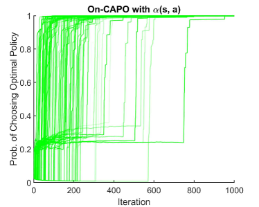
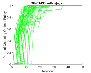
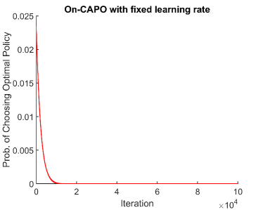
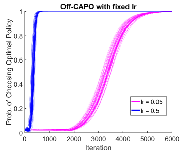
Figure 2: The probability weight of the trained policies on the optimal action at different iterations.

Appendix F Exploration Capability Provided by a Coordinate Generator in CAPO

In this section, we demonstrate empirically the exploration capability provided by the coordinate generator in CAPO.

F.1 Configuration

The Chain environment is visualized in Figure 3. This environment is meant to evaluate the agent’s ability to resist the temptation of immediate reward and look for the better long-term return. We compare the performance of Batch CAPO, Cyclic CAPO and Off-policy Actor Critic on Chain with $N=10$, and the result can be found in Figure 4. To eliminate the factor of critic estimation, true value of the value function is used during training. All the agents are trained for 1000 iterations with learning rate $=0.001$. The policies are represented by a neural network with a single hidden layer (with hidden layer size 256). Both Cyclic CAPO and Off-policy Actor Critic is trained with a batch size of 16 and a replay buffer size of 100. As Batch CAPO shall take all the $\mathcal{S}\mathcal{A}$-pairs into account by design, the effective batch size of Batch CAPO is equal to $\mathcal{S}\times\mathcal{A}$. Unlike the CAPO methods, Off-policy Actor Critic presumes the use of a fixed behavior policy. As a result, similar to the experimental setup of various prior works (e.g., (Liu et al., 2020b)), we use a uniform behavior policy for Off-policy Actor Critic. The use of a fixed behavior policy makes it difficult to identify an optimal policy, and this highlights the benefit of a coordinate generator in terms of exploration.

F.2 Discussion

From Figure 4 we can see that it is difficult for Off-policy Actor Critic to escape from a sub-optimal policy, despite that the true value of the value function is provided. Since both Cyclic CAPO and Batch CAPO satisfy 1, using such coordinate selection rules provides sufficient exploration for CAPO to identify the optimal policy. This feature can be particularly useful when the reward is sparse and the trajectory is long.

Figure 3: The Chain environment has a total of $n+1$ states, and the agent always starts at state $1$. The agent has two actions to choose from at every state, either receive a reward of $0.1$ and terminate immediately, or move one state to the right. While moving right will receive no reward in most states, the transition from $S_{n-1}$ to $S_{n}$ would induce a huge reward of $100$. A well-performing policy should prefer the delayed reward of 100 over the immediate reward of 0.1.

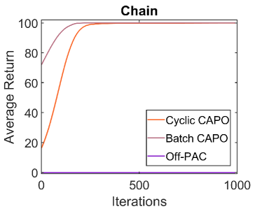
Figure 4: Comparison between Cyclic CAPO, Batch CAPO and off-policy Actor Critic, where the result is the average over 30 runs. We can see that despite the true value function is given and the optimal reward is much larger than the immediate reward (100 v.s. 0.1), Off-policy Actor Critic still suffers from a sub-optimal policy.

Appendix G Detailed Configuration of Experiments

G.1 Implementation Detail

Algorithm 3 shows the pseudo code of NCAPO. In order to demonstrate the off-policy capability of NCAPO, we use simple $\epsilon$-greedy with initial exploration $\epsilon_{start}$ and decayed exploration for off-policy exploration and estimates $A(s,a)$ with Retrace Munos et al. (2016). NCAPO uses four simple 2-layer feed-forward neural networks, a behavior network ($\theta^{b}$), a target network ($\theta$), a critic network ($\theta^{Q}$) and a target critic network ($\theta^{Q^{\prime}}$). In each episode, $N_{\text{rollouts}}$ rollouts are collected, and each rollout $r=[(s_{t},a_{t}),...,(s_{t+l},a_{t+l})]$ has length of $l$. Note that instead of storing a single $(s,a)$-pair in the replay buffer $R$, we store the entire rollout of length $l$ into $R$ to better compute $Q_{\text{retrace}}$. Due to the limited representation capability of floating-point numbers, during the CAPO update, the term $\log\frac{1}{\pi}$ can grow unbounded as $\pi\rightarrow 0$. To address this, we clip the term so that $\alpha(s,a)=\min(\log\frac{1}{\pi(a\mid s)},\text{clip})$. As the target networks have demonstrated the ability to stabilize training, the target networks are used and updated by polyak average update with coefficient $\tau_{\theta}$ and $\tau_{Q}$. The experiment is conducted on a computational node equipped with Xeon Platinum 8160M CPU with a total of 40 cores. Off-PAC shares a similar code base as NCAPO, the major difference is that the use of a fixed behavior policy. We choose such behavior policy to be a uniform policy.

G.2 Hyperparameters

We use the hyperparameters for Atari games of stable-baseline3 for (Raffin et al., 2019) for PPO and A2C, and the exact same hyperparameter from (Obando-Ceron and Castro, 2021) for Rainbow. The hyperparameters are listed in Table 2.

Table 2: Hyperparameters for CAPO and OffPAC

Hyperparameters	CAPO	PPO	A2C	OffPAC
batch size	32	16	-	32
learning rate	5e-4	2.5e-4	7e-4	5e-4
exploration fraction	10%	0	0	10%
Initial exploration rate*	0.3	0	0	0
Final exploration rate	0.05	0	0	0
Critic loss coefficient*	1	0.38	0.25	1
max gradient norm	0.8	0.5	0.5	0.8
gradient steps	30	1	1	30
train frequency	(64, steps)	(256, steps)	-	(64, steps)
$\tau_{Q}$	0.05	-	-	0.05
$\tau_{\theta}$	1	-	-	1
gamma	0.99	0.98	0.99	0.99
replay buffer	6400	-	-	6400
clip value	50	-	-	-
entropy coef	0	-	4.04e-6	0

For Asterix, the critic loss coefficient is $0.25$ and the initial exploration rate is $0.8$.

Appendix H Pseudo Code of the Proposed Algorithms

Algorithm 1 Coordinate Ascent Policy Optimization

1:  Initialize policy $\pi_{\theta}$, $\theta\in\mathcal{S}\times\mathcal{A}$

2:  for $m=1,\cdots,M$ do

3:     Generate $|\mathcal{B}|$ state-action pairs $((s_{0},a_{0}),...,(s_{|\mathcal{B}|},a_{|\mathcal{B}|}))$ from some coordinate selection rule satisfying 1.

4:     for $i=1,\cdots,|\mathcal{B}|$ do

5:        $\theta_{m+1}(s_{i},a_{i})\leftarrow\theta_{m}(s_{i},a_{i})+\alpha_{m}(s_{i},a_{i})\operatorname{sign}\left(A^{m}(s_{i},a_{i})\right)$

6:     end for

7:  end for

Algorithm 2 Neural Coordinate Ascent Policy Optimization

1:  Initialize actor network $f_{\theta}$, where policy is parameterized as $\pi_{\theta}(a|s)=\frac{f_{\theta}(s,a)}{\sum_{a^{\prime}\in\mathcal{A}}f_{\theta}(s,a^{\prime})}$

2:  for $m=1,\cdots,M$ do

3:     Generate state-action pairs $\left((s_{0},a_{0}),...,(s_{|\mathcal{B}|},a_{|\mathcal{B}|}\right))$ from some coordinate selection rule satisfying 1.

4:     Evaluate Advantage $A^{\pi_{m}}$ with arbitrary policy evaluation algorithm.

5:     Compute target $\hat{\theta}$ by (18).

6:     Compute target policy $\hat{\pi}$ by taking softmax over $\hat{\theta}$.

7:     Update the policy network with NCAPO loss:

8:     $\nabla_{\theta}L=\nabla_{\theta}D_{KL}\left(\pi_{f_{\theta_{m}}}\|\hat{\pi}\right)$

9:  end for

Algorithm 3 Neural Coordinate Ascent Policy Optimization with Replay Buffer

1:  Initialize behavior network $f(s,a\mid\theta^{b})$, critic $Q(s,a\mid\theta^{Q})$

2:  Initialize Replay Buffer $R$,

3:  Initialize target networks $f(s,a\mid\theta)\leftarrow f(s,a\mid\theta^{b})$, $Q(s,a|\theta^{Q^{\prime}})\leftarrow Q(s,a|\theta^{Q})$

4:  for episode $m=1,\cdots,M$ do

5:     Generate behavior policy and target policy by computing softmax $\pi_{\theta}(a\mid s)=\frac{e^{f(s,a\mid\theta)}}{\sum_{a^{\prime}\in\mathcal{A}}e^{f\left(s,a^{\prime}\mid\theta\right)}}$.

6:     Collect $N_{rollouts}$ rollouts with length $l$ by following $\pi_{\theta_{b}}$ with decayed ${\epsilon}$-greedy, store rollouts to $R$.

7:     Replace old rollouts if $len(R)>R_{max}$ .

8:     for gradient steps $=1,...,\mathcal{G}$ do

9:        Sample rollout $r$ from $R$.

10:        Compute $Q_{retrace}(s,a)$ for $(s,a)\in r$

11:        $\theta^{Q}_{Loss}\leftarrow\sum_{(s,a)\in r}(Q_{retrace}(s,a)-Q_{\theta^{Q}}(s,a))^{2}$

12:        $\theta_{Loss}\leftarrow D_{KL}\left(\pi_{m}(\cdot\mid s)\mid\pi_{\hat{\theta}}(\cdot\mid s\right)$

13:        Update $Q(s,a\mid\theta^{Q})$ with gradient $\nabla_{\theta^{Q}}\theta^{Q}_{Loss}$

14:        Update $f(s,a\mid\theta^{b})$ with gradient $\nabla_{\theta}\theta_{Loss}$

15:     end for

16:     Update target networks: $\theta^{Q^{\prime}}\leftarrow\tau_{Q}\theta^{Q}+(1-\tau_{Q})\theta^{Q^{\prime}}$ $\theta\leftarrow\tau_{\theta}\theta^{b}+(1-\tau_{\theta})\theta$

17:  end for

References

- Degris et al. (2012) Thomas Degris, Martha White, and Richard S Sutton. Off-Policy Actor-Critic. In International Conference on Machine Learning, pages 179–186, 2012.
- Lillicrap et al. (2016) Timothy P Lillicrap, Jonathan J Hunt, Alexander Pritzel, Nicolas Heess, Tom Erez, Yuval Tassa, David Silver, and Daan Wierstra. Continuous control with deep reinforcement learning. In International Conference on Learning Representations, 2016.
- Gu et al. (2017a) Shixiang Gu, Timothy Lillicrap, Zoubin Ghahramani, Richard E Turner, and Sergey Levine. Q-Prop: Sample-Efficient Policy Gradient with An Off-Policy Critic. In International Conference on Learning Representations, 2017a.
- Mnih et al. (2016) Volodymyr Mnih, Adrià Puigdomènech Badia, Mehdi Mirza, Alex Graves, Timothy P. Lillicrap, Tim Harley, David Silver, and Koray Kavukcuoglu. Asynchronous methods for deep reinforcement learning, 2016.
- Agarwal et al. (2019) Alekh Agarwal, Sham M Kakade, Jason D Lee, and Gaurav Mahajan. On the theory of policy gradient methods: Optimality, approximation, and distribution shift. arXiv:1908.00261, 2019.
- Bhandari and Russo (2019) Jalaj Bhandari and Daniel Russo. Global optimality guarantees for policy gradient methods. arXiv:1906.01786, 2019.
- Mei et al. (2020) Jincheng Mei, Chenjun Xiao, Csaba Szepesvari, and Dale Schuurmans. On the global convergence rates of softmax policy gradient methods. In International Conference on Machine Learning, pages 6820–6829, 2020.
- Cen et al. (2022) Shicong Cen, Chen Cheng, Yuxin Chen, Yuting Wei, and Yuejie Chi. Fast global convergence of natural policy gradient methods with entropy regularization. Operations Research, 70(4):2563–2578, 2022.
- Liu et al. (2020a) Yanli Liu, Kaiqing Zhang, Tamer Basar, and Wotao Yin. An improved analysis of (variance-reduced) policy gradient and natural policy gradient methods. Advances in Neural Information Processing Systems, 33:7624–7636, 2020a.
- Mei et al. (2021) Jincheng Mei, Bo Dai, Chenjun Xiao, Csaba Szepesvari, and Dale Schuurmans. Understanding the effect of stochasticity in policy optimization. Advances in Neural Information Processing Systems, 34:19339–19351, 2021.
- Chung et al. (2021) Wesley Chung, Valentin Thomas, Marlos C Machado, and Nicolas Le Roux. Beyond variance reduction: Understanding the true impact of baselines on policy optimization. In International Conference on Machine Learning, pages 1999–2009, 2021.
- Imani et al. (2018) Ehsan Imani, Eric Graves, and Martha White. An off-policy policy gradient theorem using emphatic weightings. Advances in Neural Information Processing Systems, 31, 2018.
- Maei (2018) Hamid Reza Maei. Convergent actor-critic algorithms under off-policy training and function approximation. arXiv:1802.07842, 2018.
- Wang et al. (2017) Ziyu Wang, Victor Bapst, Nicolas Heess, Volodymyr Mnih, Remi Munos, Koray Kavukcuoglu, and Nando de Freitas. Sample efficient actor-critic with experience replay. In International Conference on Learning Representations, 2017.
- Gu et al. (2017b) S Gu, T Lillicrap, Z Ghahramani, RE Turner, B Schölkopf, and S Levine. Interpolated Policy Gradient: Merging On-Policy and Off-Policy Gradient Estimation for Deep Reinforcement Learning. Advances in Neural Information Processing Systems, 2017:3847–3856, 2017b.
- Ciosek and Whiteson (2018) Kamil Ciosek and Shimon Whiteson. Expected policy gradients. In Proceedings of the AAAI Conference on Artificial Intelligence, volume 32, 2018.
- Espeholt et al. (2018) Lasse Espeholt, Hubert Soyer, Remi Munos, Karen Simonyan, Vlad Mnih, Tom Ward, Yotam Doron, Vlad Firoiu, Tim Harley, Iain Dunning, et al. IMPALA: Scalable Distributed Deep-RL With Importance Weighted Actor-Learner Architectures. In International Conference on Machine Learning, pages 1407–1416, 2018.
- Liu et al. (2020b) Yao Liu, Adith Swaminathan, Alekh Agarwal, and Emma Brunskill. Off-policy policy gradient with stationary distribution correction. In Uncertainty in Artificial Intelligence, pages 1180–1190, 2020b.
- Zhang et al. (2020) Shangtong Zhang, Bo Liu, Hengshuai Yao, and Shimon Whiteson. Provably convergent two-timescale off-policy actor-critic with function approximation. In International Conference on Machine Learning, pages 11204–11213, 2020.
- Nesterov (2012) Yu Nesterov. Efficiency of Coordinate Descent Methods on Huge-Scale Optimization Problems. SIAM Journal on Optimization, 22(2):341–362, 2012.
- Singh et al. (2000) Satinder Singh, Tommi Jaakkola, Michael L Littman, and Csaba Szepesvári. Convergence Results for Single-Step On-Policy Reinforcement-Learning Algorithms. Machine learning, 38(3):287–308, 2000.
- Munos et al. (2016) Remi Munos, Tom Stepleton, Anna Harutyunyan, and Marc Bellemare. Safe and Efficient Off-Policy Reinforcement Learning. Advances in Neural Information Processing Systems, 29:1054–1062, 2016.
- Young and Tian (2019) Kenny Young and Tian Tian. MinAtar: An Atari-Inspired Testbed for Thorough and Reproducible Reinforcement Learning Experiments. arXiv:1903.03176, 2019.
- Sutton et al. (1999) Richard S Sutton, David McAllester, Satinder Singh, and Yishay Mansour. Policy gradient methods for reinforcement learning with function approximation. Advances in Neural Information Processing Systems, 12, 1999.
- Zhang et al. (2019) Shangtong Zhang, Wendelin Boehmer, and Shimon Whiteson. Generalized off-policy actor-critic. Advances in Neural Information Processing Systems, 32, 2019.
- Saha and Tewari (2013) Ankan Saha and Ambuj Tewari. On the Nonasymptotic Convergence of Cyclic Coordinate Descent Methods. SIAM Journal on Optimization, 23(1):576–601, 2013.
- Tseng (2001) Paul Tseng. Convergence of a Block Coordinate Descent Method for Nondifferentiable Minimization. Journal of optimization theory and applications, 109(3):475–494, 2001.
- Beck and Tetruashvili (2013) Amir Beck and Luba Tetruashvili. On the convergence of block coordinate descent type methods. SIAM journal on Optimization, 23(4):2037–2060, 2013.
- Jordan et al. (1999) Michael I Jordan, Zoubin Ghahramani, Tommi S Jaakkola, and Lawrence K Saul. An introduction to variational methods for graphical models. Machine learning, 37(2):183–233, 1999.
- Kakade (2001) Sham M Kakade. A natural policy gradient. Advances in Neural Information Processing Systems, 14, 2001.
- Khodadadian et al. (2021a) Sajad Khodadadian, Prakirt Raj Jhunjhunwala, Sushil Mahavir Varma, and Siva Theja Maguluri. On the linear convergence of natural policy gradient algorithm. In IEEE Conference on Decision and Control (CDC), pages 3794–3799, 2021a.
- Ji et al. (2021) Geng Ji, Debora Sujono, and Erik B Sudderth. Marginalized stochastic natural gradients for black-box variational inference. In International Conference on Machine Learning, pages 4870–4881, 2021.
- Ilyas et al. (2019) Andrew Ilyas, Logan Engstrom, Shibani Santurkar, Dimitris Tsipras, Firdaus Janoos, Larry Rudolph, and Aleksander Madry. A closer look at deep policy gradients. In International Conference on Learning Representations, 2019.
- Cutler et al. (2014) Mark Cutler, Thomas J Walsh, and Jonathan P How. Reinforcement learning with multi-fidelity simulators. In IEEE International Conference on Robotics and Automation (ICRA), pages 3888–3895, 2014.
- Kandasamy et al. (2016) Kirthevasan Kandasamy, Gautam Dasarathy, Barnabas Poczos, and Jeff Schneider. The multi-fidelity multi-armed bandit. Advances in Neural Information Processing Systems, 29, 2016.
- Khairy and Balaprakash (2022) Sami Khairy and Prasanna Balaprakash. Multifidelity reinforcement learning with control variates. arXiv:2206.05165, 2022.
- Hessel et al. (2018) Matteo Hessel, Joseph Modayil, Hado Van Hasselt, Tom Schaul, Georg Ostrovski, Will Dabney, Dan Horgan, Bilal Piot, Mohammad Azar, and David Silver. Rainbow: Combining improvements in deep reinforcement learning. In Thirty-second AAAI conference on artificial intelligence, 2018.
- Obando-Ceron and Castro (2021) Johan S Obando-Ceron and Pablo Samuel Castro. Revisiting rainbow: Promoting more insightful and inclusive deep reinforcement learning research. In Proceedings of the 38th International Conference on Machine Learning, Proceedings of Machine Learning Research. PMLR, 2021.
- Schulman et al. (2017) John Schulman, Filip Wolski, Prafulla Dhariwal, Alec Radford, and Oleg Klimov. Proximal policy optimization algorithms. arXiv:1707.06347, 2017.
- Raffin et al. (2019) Antonin Raffin, Ashley Hill, Maximilian Ernestus, Adam Gleave, Anssi Kanervisto, and Noah Dormann. Stable baselines3. https://github.com/DLR-RM/stable-baselines3, 2019.
- Silver et al. (2014) David Silver, Guy Lever, Nicolas Heess, Thomas Degris, Daan Wierstra, and Martin Riedmiller. Deterministic policy gradient algorithms. In International conference on machine learning, pages 387–395, 2014.
- Schmitt et al. (2020) Simon Schmitt, Matteo Hessel, and Karen Simonyan. Off-Policy Actor-Critic With Shared Experience Replay. In International Conference on Machine Learning, pages 8545–8554, 2020.
- Khodadadian et al. (2021b) Sajad Khodadadian, Zaiwei Chen, and Siva Theja Maguluri. Finite-sample analysis of off-policy natural actor-critic algorithm. In International Conference on Machine Learning, pages 5420–5431, 2021b.
- Chen and Maguluri (2022) Zaiwei Chen and Siva Theja Maguluri. Sample complexity of policy-based methods under off-policy sampling and linear function approximation. In International Conference on Artificial Intelligence and Statistics, pages 11195–11214, 2022.
- Chen et al. (2022) Zaiwei Chen, Sajad Khodadadian, and Siva Theja Maguluri. Finite-sample analysis of off-policy natural actor–critic with linear function approximation. IEEE Control Systems Letters, 6:2611–2616, 2022.
- Xu et al. (2021) Tengyu Xu, Zhuoran Yang, Zhaoran Wang, and Yingbin Liang. Doubly robust off-policy actor-critic: Convergence and optimality. In International Conference on Machine Learning, pages 11581–11591, 2021.
- Huang and Jiang (2022) Jiawei Huang and Nan Jiang. On the convergence rate of off-policy policy optimization methods with density-ratio correction. In International Conference on Artificial Intelligence and Statistics, pages 2658–2705, 2022.
- Laroche and Tachet des Combes (2021) Romain Laroche and Remi Tachet des Combes. Dr Jekyll & Mr Hyde: the strange case of off-policy policy updates. Advances in Neural Information Processing Systems, 34:24442–24454, 2021.
- Laroche and Des Combes (2022) Romain Laroche and Remi Tachet Des Combes. Beyond the policy gradient theorem for efficient policy updates in actor-critic algorithms. In International Conference on Artificial Intelligence and Statistics, pages 5658–5688, 2022.
- Van Hasselt and Wiering (2007) Hado Van Hasselt and Marco A Wiering. Reinforcement Learning in Continuous Action Spaces. In IEEE International Symposium on Approximate Dynamic Programming and Reinforcement Learning, pages 272–279, 2007.
- Zimmer et al. (2016) Matthieu Zimmer, Yann Boniface, and Alain Dutech. Neural Fitted Actor-Critic. In European Symposium on Artificial Neural Networks, Computational Intelligence and Machine Learning (ESANN 2016), 2016.
- Zimmer and Weng (2019) Matthieu Zimmer and Paul Weng. Exploiting the sign of the advantage function to learn deterministic policies in continuous domains. In International Joint Conferences on Artificial Intelligence, 2019.
- Tessler et al. (2019) Chen Tessler, Guy Tennenholtz, and Shie Mannor. Distributional Policy Optimization: An Alternative Approach for Continuous Control. Advances in Neural Information Processing Systems, 32:1352–1362, 2019.
- Kakade and Langford (2002) Sham Kakade and John Langford. Approximately optimal approximate reinforcement learning. In International Conference on Machine Learning, 2002.