Progressive Multi-view Human Mesh Recovery with Self-Supervision

Abstract

To date, little attention has been given to multi-view 3D human mesh estimation, despite real-life applicability (e.g., motion capture, sport analysis) and robustness to single-view ambiguities. Existing solutions typically suffer from poor generalization performance to new settings, largely due to the limited diversity of image-mesh pairs in multi-view training data. To address this shortcoming, people have explored the use of synthetic images. But besides the usual impact of visual gap between rendered and target data, synthetic-data-driven multi-view estimators also suffer from overfitting to the camera viewpoint distribution sampled during training which usually differs from real-world distributions. Tackling both challenges, we propose a novel simulation-based training pipeline for multi-view human mesh recovery, which (a) relies on intermediate 2D representations which are more robust to synthetic-to-real domain gap; (b) leverages learnable calibration and triangulation to adapt to more diversified camera setups; and (c) progressively aggregates multi-view information in a canonical 3D space to remove ambiguities in 2D representations. Through extensive benchmarking, we demonstrate the superiority of the proposed solution especially for unseen in-the-wild scenarios.

Introduction

As a key step to several human-centric applications, 3D human mesh estimation from multi-view images has shown superiority beyond monocular image as it eliminates common ambiguities among single-image scenarios. Most successes in 3D human mesh recovery are demonstrated by supervised training. However, such models hardly generalize to in-the-wild scenarios due to the lack of sufficient and diverse 3D annotations paired with multi-view images. Generalizability of human mesh estimation models developed using supervision on large-scale in-studio datasets remains questionable, as these models often perform unsatisfactorily on unseen in-the-wild environments. Though weakly-supervised models can be an option to address this shortcoming, their performance highly relies on availability and diversity of unpaired 2D/3D annotations or temporal/multi-view image pairs, therefore limiting generalization capability.

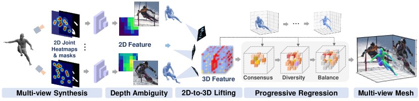
Figure 1: (1) Our method is purely synthetic-data-driven regressing human mesh from 2D representations. During training 2D representations are acquired from synthetic mesh rendering. During testing 2D representations are predicted with off-the-shelf detectors. The existing well-trained 2D detectors equip our method with better generalizability and robustness to in-the-wild scenarios. (2) By unifying multi-view knowledge in canonical 3D space, we explicitly explore consensus, diversity and balance to deal with the inherent inconsistency among different views.

When collected training data are insufficient and infeasible to generalize, simulated training data can be a useful alternative. Works have been done to synthetically generate and render images of human bodies for dense pose estimation (Zhu, Karlsson, and Bregler 2020), depth estimation (Varol et al. 2017), 3D pose estimation (Rogez and Schmid 2016; Varol et al. 2017; Kundu et al. 2020; Patel et al. 2021), 3D human reconstruction (Zheng et al. 2019; Sengupta, Budvytis, and Cipolla 2020; Yu et al. 2021). Most of the self-supervised approaches only focus on single view tasks. Although works such as Kocabas, Karagoz, and Akbas (2019); Wandt et al. (2021) employ multi-view geometry for self-supervised training, for testing they infer on individual images independently, even when multi-view data are available. We believe that there commonly exist multi-view images in real scenarios, but self-supervised multi-view human pose/mesh estimation remains relatively unexplored.

Some works have taken steps to eliminate the requirements of 3D human mesh annotation. Pavlakos et al. (2017b) explore 3D geometry of the camera setup to lift from multi-view 2D joints to 3D pictorial structure. But the training process highly relies on multi-view imagery and only estimate human pose excluding human shape. Liang and Lin (2019) generate multi-view human RGB images from existing SMPL (Loper et al. 2015) pose and shape parameters. But its synthetic paired data only helps to improve the performance of model trained with real image-3D annotations. Although these works have deliberately designed human textures, light, background during rendering, the model only trained with its synthetic data can hardly generalize to real scenarios due to the domain gap between real and synthetic images. It is obvious that the rendered images can hardly generalize to the real images in the wild.

On the other hand, proxy representations (e.g., joints, silhouettes) are commonly used as intermediate representation in human mesh recovery (HMR) task, and can serve as good transition to bridge RGB image and SMPL parameters: 1) synthetic-to-real domain gap is smaller for proxy representation, thus can be more easily bridged; 2) a vast amount of SMPL parameters can be rendered into proxy representations to formulate paired synthetic data; 3) there exist multiple well-trained models predicting image to these 2D lower-dimensionality representations, which are relatively more robust and generalized compared with 3D mesh predictors.

To this point, we propose to train with multi-view synthetic data for multi-view human mesh estimation. Compared to single-view synthetic training (Pavlakos et al. 2018; Sengupta, Budvytis, and Cipolla 2020; Yu et al. 2021; Gong et al. 2022; Zheng et al. 2022), two challenges specific to multi-view synthetic training arise. First, an additional domain gap between the real testing data and synthetic training data can be easily introduced due to inconsistency between the testing camera viewpoint distribution and the synthetic training viewpoints. Due to the lack of available multi-view SMPL parameters and camera calibration, the sampling of camera setups for multi-view synthesis should generalize to real multi-view settings which can be quite diverse across different datasets. The second challenge comes from the inherent inconsistency among multi-view representations in real scenarios. Limited by occlusion and depth ambiguity, 2D representations inferred from testing images are more likely to be biased from 3D ground-truth when compared with images which are used in those fully supervised multi-view methods.

To address the aforementioned issues, we propose a novel synthetic-data-driven training pipeline (Figure 1) for multi-view human mesh recovery. 1) We synthetically train a regression model from multi-view 2D representations to SMPL parameters. During inference off-the-shelf detection/segmentation models are used to predict these 2D representations from RGB images. 2) The viewpoint setup for synthetic training is consistent with real testing scenarios via learnable volumetric triangulation and calibration. 3) Multi-view 2D representations are aggregated in the shared 3D human space and progressively regressed to deal with the possible bias existing in 2D representation. As illustrated in Figure 2, we aim to let the regressor first focus on the consensual key area and then learn from the possible highlighted area for diversity. Once we get mesh prediction from these two regression iterations, we are able to better balance the multi-view volumetric features via reprojection consistency where views less consistent with the predicted mesh will be given less weight in the final mesh refinement iteration. Empirical evaluations show that our method achieves very competitive results on H3.6M (Ionescu et al. 2013), TotalCapture (Trumble et al. 2017) and challenging SkiPose (Spörri 2016; Rhodin et al. 2018) dataset compared with other fully/weakly supervised multi-view human mesh recovery and human pose estimation methods.

Our key contributions can be summarized as: 1) We propose a multi-view synthetic-data-driven training pipeline for multi-view human mesh recovery, mapping multi-view 2D representations to shared 3D human space to bridge the real-synthetic gap. 2) We progressively regress multi-view representations by first exploring the consensus and diversity among views in 3D space and then reaching evidential balance among views. This design can efficiently tolerate the bias commonly existing in single 2D representation thus generalizable to in-the-wild scenarios. 3) We conduct extensive experiments on standard benchmark datasets and demonstrate comparable numbers with fully/weakly supervised methods on conventional evaluation metrics.

Related Works

Monocular 3D Human Pose Estimation: 3D human pose estimation (HPE) (Agarwal and Triggs 2005; Song et al. 2021) problem can be categorized into 3D body keypoint/skeleton prediction and 3D human mesh recovery, based on representing the human body with kinematic or volumetric models. 3D keypoint/skeleton prediction can be further divided into: 1) end-to-end estimation models that output 3D keypoint locations given monocular images (Pavlakos et al. 2017a; Pavlakos, Zhou, and Daniilidis 2018; Sun et al. 2018; Li, Zhang, and Chan 2015); 2) two-stage 2D-to-3D lifting schemes that first estimate 2D human keypoints and then lift to 3D space (Chen and Ramanan 2017; Li and Lee 2019; Martinez et al. 2017; Zhou et al. 2019a; Su et al. 2022). The latter solutions typically outperform end-to-end ones by leveraging superior performance and generalizability of off-the-shelf 2D keypoint detectors. On the other hand, 3D human mesh recovery (HMR) (Loper et al. 2015) regresses and outputs mesh parameters, containing richer shape and texture information of the human body. Recently, numerous methods (Kolotouros et al. 2019; Arnab, Doersch, and Zisserman 2019; Bogo et al. 2016; Li et al. 2021) focus on estimating parameters of the Skinned Multi-Person Linear (SMPL) (Loper et al. 2015), a commonly-used volumetric human model with high compatibility, to statistically regress human meshes. Several works take steps to leverage a variety of easily-obtained clues, i.e., weak supervision, such as paired 2D landmarks and silhouettes (Tan, Budvytis, and Cipolla 2017; Pavlakos et al. 2018; Kanazawa et al. 2018; Rong et al. 2019; Wehrbein et al. 2021).

Multi-view 3D Human Pose Estimation Many methods (Dong et al. 2019; Liang and Lin 2019; Qiu et al. 2019; Rhodin, Salzmann, and Fua 2018; Pavlakos et al. 2017b; Zhang et al. 2021) have recently proposed for multi-view 3D HPE. While the majority focuses on 3D body keypoint/skeleton prediction (Pavlakos et al. 2017b; Dong et al. 2019; Rhodin, Salzmann, and Fua 2018), we consider the problem of multi-view 3D HMR, which reconstructs 3D SMPL (Loper et al. 2015) pose and shape parameters given multiple view images. Existing multi-view HMR methods are all supervised, fusing multi-view with probabilistic modeling (Kolotouros et al. 2021) or collaborative learning (Li, Oskarsson, and Heyden 2021) to regress SMPL parameters. Liang and Lin (2019) uses additional synthetic image-SMPL pairs to train a multi-view multi-stage regression network. (Dong et al. 2021) aggregates multi-view observation based on confidence-aware majority voting technique.

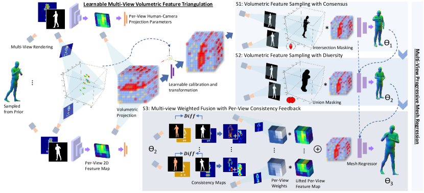
Figure 2: Overall illustration of the proposed pipeline. We unproject the 2D occupancy maps to 3D space to obtain intersection and union of 3D occupancy used to mask the volumetric features. The intersection and union masking in 3D space help to sample volumetric features according to multi-view consensus and diversity respectively. This progressive regression design can efficiently tolerate possible bias and seek consistency in real multi-view settings.

Method

Prerequisites

3D human mesh parameterization: Skinned Multi-Person Linear (SMPL) (Loper et al. 2015) is a parametric model providing independent body shape $\bm{\beta}$ and pose $\bm{\theta}$ parameters with very low-dimensional parameters (i.e., $\bm{\beta}\in\mathbb{R}^{10}$ and $\bm{\theta}\in\mathbb{R}^{72}$). Pose parameters $\bm{\theta}=\{\bm{\theta}_{\text{g}},\bm{\theta}_{\text{j}}\}$ include global body rotation $\bm{\theta}_{\text{g}}$ (3-DOF) and relative 3D rotations of 23 joints $\bm{\theta}_{\text{j}}$ (23$\times$3-DOF) in the axis-angle format. Shape parameters include individual heights and weights indicated by the first 10 coefficients of a PCA shape space. SMPL provides a differentiable kinematic function $\mathcal{S}$ from $\{\bm{\theta},\bm{\beta}\}$ to 6,890 mesh vertices: $\bm{v}=\mathcal{S}(\bm{\theta},\bm{\beta})\in\mathbb{R}^{6890\times 3}$. Besides, 3D locations for $N_{\text{J}}$ joints of interest are obtained as $\bm{j}^{\text{3D}}=\mathcal{J}\bm{v}$, where $\mathcal{J}\in\mathbb{R}^{N_{\text{J}}\times 6890}$ is a linear regression matrix.

Monocular training data synthesis: Existing synthetic based HMR methods (Sengupta, Budvytis, and Cipolla 2020; Sengupta, Budvytis, and Cipolla 2021b, a) generate paired 2D representations (i.e., binary mask, edge and 2D joints) and 3D meshes with SMPL parameters on the fly during training process. At each training step, pose $\{\bm{\theta}_{\text{g}},\bm{\theta}_{\text{j}}\}$ and shape $\bm{\beta}$ are sampled from MoCap (C 2003; Rogez and Schmid 2016) datasets and prior statistical normal distribution respectively. The camera translation $\bm{T}\in\mathbb{R}^{3}$ is also dynamically sampled from prior distribution. The intrinsic parameters are fixed and represented by focal length $\bm{f}\in\mathbb{R}^{2}$ and image center offset $\bm{t}=[H/2,W/2]$, where $H$, $W$ is rendered image size. $\{\bm{\theta}_{\text{g}},\bm{\theta}_{\text{j}},\bm{\beta}\}$ are forwarded into the SMPL model to obtain 3D joints $\bm{j}_{\text{3D}}$. 2D joints $\bm{j}_{\text{2D}}$ can be acquired by $\bm{j}_{\text{2D}}=\bm{f}\mathbf{\Pi}(\bm{j}_{\text{3D}}+\bm{T})+\bm{t}$, where $\mathbf{\Pi}$ denotes perspective projection. The 2D joints $\bm{j}_{\text{2D}}\in\mathbb{R}^{N_{\text{J}}\times 2}$ are transformed into 2D Gaussian joint heatmaps $\bm{J}\in\mathbb{R}^{N_{\text{J}}\times H\times W}$. Another 2D proxy representation, human mask, can be represented by $\bm{M}\in\mathbb{R}^{H\times W}$. The training model utilizes the synthesized paired data with 2D representations $\{\bm{J},\bm{M}\}$ as input and 3D meshes $\{\bm{\theta},\bm{\beta},\bm{v},\bm{j}_{\text{3D}}\}$ as output.

Volumetric triangulation: Beyond basic algebraic triangulation, volumetric triangulation (Iskakov et al. 2019) is able to unproject multi-view 2D features along projection rays to fill a shared 3D cube. The cube is a $L\times L\times L$ - sized 3D bounding box in the global space discretized by $G\times G\times G$ volumetric grids, where $G$ represents the number of voxels along each axis. Then each voxel is filled with the global coordinates of the voxel center to get $\bm{V}^{\text{coords}}\in\mathbb{R}^{G\times G\times G\times 3}$. $\bm{V}^{\text{coords}}$ is projected to the image plan to get its corresponding 2D pixel index $\bm{V}^{\text{proj}}\in\mathbb{R}^{G\times G\times G\times 2}$. Given 2D maps $\bm{F}\in\mathbb{R}^{C\times H\times W}$ in image space, we can fill a cube $\bm{V}\in\mathbb{R}^{G\times G\times G\times C}$ by bilinear sampling (Jaderberg et al. 2015) using $\bm{V}^{\text{proj}}$. The whole process is differentiable and agnostic to the number of views.

Multi-view Training Data Synthesis

As described above, the synthesis of 2D proxy representations relies on camera extrinsic parameters $\{\bm{R}_{\text{h}\rightarrow\text{c}},\bm{T}_{\text{h}\rightarrow\text{c}}\}$ (the transformation between human coordinate and camera coordinate) for each camera. The intuitive solution of multi-view synthesis is to randomly sample multi-view camera extrinsic parameters around the human body. But the lack of statistical priors makes it not ideal since some views (e.g., from below the human body) can never happen in real scenarios. It also requires manual tuning to ensure as much visible space as possible to avoid large area of blind spot.

We first sample one camera setting $\{\bm{R}_{\text{h}\rightarrow\text{c}^{1}},\bm{T}_{\text{h}\rightarrow\text{c}^{1}}\}$ from prior and then extend it to $N$ cameras according to the transformations among cameras in real scenarios. Though there exists no direct information, w.r.t., relations among camera setups, it can be inferred from the public camera calibrations for multi-view datasets (Ionescu et al. 2013; Trumble et al. 2017). Given $\{\bm{R}_{\text{w}\rightarrow\text{c}^{n}},\bm{T}_{\text{w}\rightarrow\text{c}^{n}}\}(n=1...N)$ as the rotation and translation from canonical world coordinate to the $n$-th camera coordinate, we calculate the transformation from the first camera to the other cameras:

$$\bm{R}_{\text{c}^{1}\rightarrow\text{c}^{n}}=\bm{R}_{\text{w}\rightarrow\text{c}^{n}}\cdot(\bm{R}_{\text{w}\rightarrow\text{c}^{1}})^{\text{T}},$$ (1)

$$\bm{T}_{\text{c}^{1}\rightarrow\text{c}^{n}}=\bm{T}_{\text{w}\rightarrow\text{c}^{n}}-\bm{R}_{\text{c}^{1}\rightarrow\text{c}^{n}}\cdot\bm{T}_{\text{w}\rightarrow\text{c}^{1}}~{}(n=2...N).$$

Utilizing these priors ensures that our synthetically trained model can better generalize to different testing multi-view images in the wild.

The overall multi-view synthesis process at each training step can be summarized as: (1) sample $\{\bm{\theta}_{\text{g}},\bm{\theta}_{\text{j}},\bm{\beta},\bm{T}\}$ following the same strategy as Sengupta, Budvytis, and Cipolla (2020); (2) sample one set of camera settings $\{\bm{R}_{\text{w}\rightarrow\text{c}^{n}},\bm{T}_{\text{w}\rightarrow\text{c}^{n}}|n=1...N\}$ (e.g., $N$ from 2 to 8); (3) calculate the transformation from camera 1 to the other cameras using Eq.1; (4) regress and render 2D joints heatmaps and binary mask $\{\bm{J}^{1},\bm{M}^{1}\}$ under camera-1 using $\bm{R}_{\text{h}\rightarrow\text{c}^{1}}$ (from $\bm{\theta}_{\text{g}}$) and $\bm{T}_{\text{h}\rightarrow\text{c}^{1}}$ as camera extrinsic parameters; (5) regress and render 2D representations $\{\bm{J}^{n},\bm{M}^{n}\}$ under other cameras using camera extrinsic parameters below:

$$\bm{R}_{\text{h}\rightarrow\text{c}^{n}}=\bm{R}_{\text{c}^{1}\rightarrow\text{c}^{n}}\cdot\bm{R}_{\text{h}\rightarrow\text{c}^{1}},$$ (2)

$$\bm{T}_{\text{h}\rightarrow\text{c}^{n}}=\bm{R}_{\text{h}\rightarrow\text{c}^{n}}\cdot\bm{T}_{\text{h}\rightarrow\text{c}^{1}}+\bm{T}_{\text{c}^{1}\rightarrow\text{c}^{n}}~{}(n=2...N).$$

We forward $\{\bm{0},\bm{\theta}_{\text{j}},\bm{\beta}\}$ into the SMPL statistical model and get $\{\bm{v},\bm{j}_{\text{3D}}\}$ in human coordinate system. We further transform $\{\bm{v},\bm{j}_{\text{3D}}\}$ with individual camera rotation $\bm{R}_{\text{h}\rightarrow\text{c}^{n}}$ to $\{\bm{v}^{n},\bm{j}_{\text{3D}}^{n}\}$ making it specific under each camera rotation. Then we project to 2D joints $\{\bm{J}^{n}$ and render to get binary mask $\bm{M}^{n}\}$ for each camera $n$. The training model utilizes the synthesized paired data with 2D representations $\{\bm{J}^{n},\bm{M}^{n}\}$ and 3D meshes $\{\bm{\theta}_{\text{j}},\bm{\beta},\bm{v}^{n},\bm{j}_{\text{3D}}^{n}\}$ where $\bm{\theta}_{\text{j}}$ and $\bm{\beta}$ are shared across all views. Note that the aforementioned camera extrinsic $\{\bm{R}_{\text{w}\rightarrow\text{c}^{n}},\bm{T}_{\text{w}\rightarrow\text{c}^{n}}\}$ and intrinsic matrix $\bm{K}$ will also be used in forwarding.

Learnable Volumetric Calibration

The 3D space for fusion is designed to be consistent with the human coordinate rather than world coordinate for mesh regression efficiency and model generalizability. However, for real testing images, we have no access to the transformation from human coordinate to image space which is necessary to do the volumetric triangulation. On the other hand, the camera intrinsic parameters $\bm{K}$ are always known and some testing datasets provide transformation from canonical world coordinate to camera coordinate. When this transformation is not available, we can simply define a world coordinate initialized with camera-1. The transformation between camera-1 and other cameras can be acquired from 2D joints in different views. Please refer to Kocabas, Karagoz, and Akbas (2019) for details. Based on the aforementioned known transformation from canonical world to each camera coordinate (${\bm{R}}_{\text{w}\rightarrow\text{c}^{n}}$, ${\bm{T}}_{\text{w}\rightarrow\text{c}^{n}}$), we design volumetric calibration to transform from canonical world to human coordinate ($\hat{\bm{R}}_{\text{w}\rightarrow\text{h}}$, $\hat{\bm{T}}_{\text{w}\rightarrow\text{h}}$) so that multi-view 2D space can be unified in a shared human space. Initialized with camera-1, the canonical world is first translated to be with the same origin as the human center which can be interpolated w.r.t. statistical torso length and 2D joints, and then rotated to be consistent with human global pose.

Translation estimation: Under each camera view, we obtain the 3D representation of pelvis heatmaps via volumetric triangulation (Iskakov et al. 2019). The per-voxel likelihood for pelvis is obtained by summing up multi-view 3D heatmaps. Via argmax (averaging the 3D positions of the voxels if there are multiple voxels containing the maximum value) we estimate the 3D pelvis position in world space as the translation from world origin to human origin $\hat{\bm{T}}_{\text{w}\rightarrow\text{h},\text{w}}$ under world space:

$$\hat{\bm{T}}_{\text{w}\rightarrow\text{h},\text{w}}=\text{argmax}\sum_{n}{\mathcal{V}(\bm{J}_{\text{pelvis}}^{n};{\bm{R}}_{\text{w}\rightarrow\text{c}^{n}},{\bm{T}}_{\text{w}\rightarrow\text{c}^{n}},\bm{K})},$$ (3)

where $\mathcal{V}(\cdot;\cdot)$ represents volumetric triangulation. Note we indicate all transformation by uniform sequence with rotation first and then translation, we therefore organize the transformation from human to each camera coordinate:

$$\hat{\bm{R}}_{\text{h}\rightarrow\text{c}^{n}}={\bm{R}}_{\text{w}\rightarrow\text{c}^{n}}\cdot\hat{\bm{R}}_{\text{w}\rightarrow\text{h}}^{\text{T}},$$ (4)

$$\hat{\bm{T}}_{\text{h}\rightarrow\text{c}^{n}}=\bm{T}_{\text{w}\rightarrow\text{c}^{n}}-\hat{\bm{R}}_{\text{w}\rightarrow\text{c}^{n}}\cdot\hat{\bm{T}}_{\text{w}\rightarrow\text{h},\text{w}}.$$

Rotation learning: For each camera view $n$, the encoder takes 2D joints heatmaps and binary mask $\{\bm{J}^{n},\bm{M}^{n}\}$ as input and output downsized features $\bm{F}^{n}\in\mathbb{R}^{C\times H_{0}\times W_{0}}$, where $C$ is channel size. To learn the rotation from canonical world to human, we unproject $\bm{F}^{n}$ to the corrected 3D space with human origin and world rotation (acquired by the estimated translation mentioned above). We first take average of the unprojected volumetric 3D features among views, then forward the flattened volumetric features into a fully-connected layer $\mathcal{F}_{\text{R}}$:

$$\hat{\bm{R}}_{\text{w}\rightarrow\text{h}}=\mathcal{F}_{\text{R}}(\cfrac{1}{N}\sum_{n}\mathcal{V}(\bm{F}^{n};\hat{\bm{R}}_{\text{w}\rightarrow\text{c}^{n}},\hat{\bm{T}}_{\text{h}\rightarrow\text{c}^{n}},\bm{K},\frac{H}{H_{0}},\frac{W}{W_{0}})$$ (5)

where $\frac{H}{H_{0}}$, $\frac{W}{W_{0}}$ are the scale factors from image space to its downsampled feature space. The output of the fully-connected layer is a continuous 6-dimensional representation (Zhou et al. 2019b) which can be converted to a discontinuous Euler rotation matrix $\hat{\bm{R}}_{\text{w}\rightarrow\text{h}}$. Note that both volumetric triangulation (grid sampling) and transformation are differentiable, thus $\hat{\bm{R}}_{\text{w}\rightarrow\text{h}}$ can be learned via projecting the predicted 3D mesh to 2D.

We note that the aforementioned calibration from canonical world to human is to unify diverse camera setups in common human space for efficient multi-view learning. The currently available $\bm{K}$ and $\hat{\bm{T}}_{\text{h}\rightarrow\text{c}^{n}}$ is not learnable and only a rough estimation which aims to correct the 3D cube center to be around the pelvis center. For more accurate joint learning together with the predicted 3D mesh, we employ reprojection loss with orthographic projection following Kanazawa et al. (2018). Specifically, we learn camera parameters from a fully-connected layer $\mathcal{F}_{\text{OP}}$ for individual view: $\hat{\bm{\pi}}^{n}=\mathcal{F}_{\text{OP}}(\bm{F}^{n})$, where $\hat{\bm{\pi}}^{n}=[\hat{\pi}_{\text{s}}^{n},\hat{\bm{\pi}}_{\text{t}}^{n}]$, $\hat{\pi}_{\text{s}}^{n}\in\mathbb{R}$ is the scale factor and $\hat{\bm{\pi}}_{\text{t}}^{n}\in\mathbb{R}^{2}$ is translation.

Progressive Multi-view Aggregation

From the aforementioned volumetric calibration, we are able to obtain the volumetric features $\bm{V}_{\text{F}}^{n}\in\mathbb{R}^{G\times G\times G\times C}$ for each camera-$n$ in the uniform 3D human space:

$$\bm{V}_{\text{F}}^{n}=\mathcal{V}(\bm{F}^{n};\hat{\bm{R}}_{\text{h}\rightarrow\text{c}^{n}},\hat{\bm{T}}_{\text{h}\rightarrow\text{c}^{n}},\bm{K},\frac{H}{H_{0}},\frac{W}{W_{0}}).$$ (6)

$\bm{V}_{\text{F}}^{n}$ from multiple views are fused (averaged or weighted summation), flattened, and then passed to the regressor $\mathcal{R}$ to predict pose and shape parameters $\bm{\Theta}=\{\hat{\bm{\theta}_{\text{j}}},\hat{\bm{\beta}}\}$. Note that we only predict 23 joints rotation $\hat{\bm{\theta}_{\text{j}}}$ shared by all views (excluding global root orientation) as we have learnt view-specific global orientation $\hat{\bm{R}}_{\text{h}\rightarrow\text{c}^{n}}$ in volumetric calibration.

Following the standard iterative error feedback (IEF) procedure (Kanazawa et al. 2018), we employ three iterative regressions to optimize $\bm{\Theta}$ and further propose progressive multi-view aggregation. We introduce how we progressively learn from consensus/diversity information from intersection and union occupancy mask, and then how we balance the multi-view 3D features from the consistency between consensus and diversity preserving mesh prediction.

Consensus and diversity sampling:

Under each camera-$n$, we consider all the possible nonzero areas of 2D joints heatmaps $\bm{J}^{n}$ and binary mask $\bm{M}^{n}$ as 2D occupancy mask $\bm{O}^{n}\in\{0,1\}^{H\times W}$ and then we obtain the volumetric occupancy mask in 3D human space $\bm{V}_{\text{O}}^{n}\in\{0,1\}^{G\times G\times G}$:

$$\bm{O}^{n}=\mathbf{1}((\sum\nolimits_{j=1}^{N_{\text{j}}}{\bm{J}_{j}^{n}}+\bm{M}^{n})>0),$$ (7)

$$\bm{V}_{\text{O}}^{n}=\mathcal{V}(\bm{O}^{n};\hat{\bm{R}}_{\text{h}\rightarrow\text{c}^{n}},\hat{\bm{T}}_{\text{h}\rightarrow\text{c}^{n}},\bm{K}).$$

To efficiently aggregate the volumetric occupancy masks, we take intersection of $\{\bm{V}_{\text{O}}^{n}|n=1...N\}$ as $\bm{V}_{\text{O}}^{\text{I}}$ representing the area of interest shared by all views (consensus), and take union of them as $\bm{V}_{\text{O}}^{\text{U}}$ which representing the area of interest masked by at least one view (diversity):

$$\bm{V}_{\text{O}}^{\text{I}}=\text{min}_{n}{\bm{V}_{\text{O}}^{n}},\\ ~{}\bm{V}_{\text{O}}^{\text{U}}=\text{max}_{n}{\bm{V}_{\text{O}}^{n}},\\$$ (8)

where $\bm{V}_{\text{O}}^{\text{I}},\bm{V}_{\text{O}}^{\text{U}}\in\{0,1\}^{G\times G\times G}$. To achieve consensus while also maintaining the diversity that is inherent among the multiple views, we mask the 3D volumetric features $\{\bm{V}_{\text{F}}^{n}\}$ spatial-wisely with occupancy intersection $\bm{V}_{\text{O}}^{\text{I}}$ and occupancy union $\bm{V}_{\text{O}}^{\text{U}}$ respectively:

$$\bm{V}_{\text{F}}^{\text{I}}=\bm{V}_{\text{O}}^{\text{I}}\odot{\frac{1}{N}\sum_{n}\bm{V}_{\text{F}}^{n}},\\ ~{}\bm{V}_{\text{F}}^{\text{U}}=\bm{V}_{\text{O}}^{\text{U}}\odot{\frac{1}{N}\sum_{n}\bm{V}_{\text{F}}^{n}}.\\$$ (9)

where $\odot$ is Hadamard product, and $\bm{V}_{\text{F}}^{\text{I}},\bm{V}_{\text{F}}^{\text{U}}\in\mathbb{R}^{G\times G\times G\times C}$ indicate the fused 3D features in consensus and diversity occupancy area respectively. Note that the diversity occupancy area is introduced to tolerate possible bias of one-view 3D occupancy which is easily caused by inaccurate camera calibration. We progressively forward $\bm{V}_{\text{F}}^{\text{I}},\bm{V}_{\text{F}}^{\text{U}}$ into the regressor $\mathcal{R}$ so that the regressor can first focus on the features in area commonly occupant by all views ($\bm{V}_{\text{O}}^{\text{I}}$), and then consider the features in all possible occupant areas ($\bm{V}_{\text{O}}^{\text{U}}$). The output of $\mathcal{R}$ can be represented by $\bm{\Theta}_{1}$ and $\bm{\Theta}_{2}$:

$$\bm{\Theta}_{1}=\bm{\Theta}_{0}+\mathcal{R}(\bm{V}_{\text{F}}^{\text{I}};\bm{\Theta}_{0}),\\ \bm{\Theta}_{2}=\bm{\Theta}_{1}+\mathcal{R}(\bm{V}_{\text{F}}^{\text{U}};\bm{\Theta}_{1}),\\$$ (10)

where $\bm{\Theta}_{0}$ is reposed pose and mean shape for initialization.

Multi-view balance via consistency weighting:

We take average of the multi-view 3D features for intersection and union fusion in the first two regression iteration. At the last iteration of regression we utilize the current 3D mesh prediction as evidence to seek consistency among views. Specifically, we project the 3D mesh to individual 2D image spaces for spatial-wise consistency as fusion confidence under each camera. Given the output of the regressor after the second iteration $\bm{\Theta}_{2}=\{\hat{\bm{\theta}}_{\text{j}},\hat{\bm{\beta}}\}$, SMPL takes $\{\bm{0},\hat{\bm{\theta}}_{\text{j}},\hat{\bm{\beta}}\}$ to infer 3D vertices $\hat{\bm{v}}$ and 3D joints $\hat{\bm{j}}^{\text{3D}}$. Using a differentiable renderer (Ravi et al. 2020), we generate a body mask $\hat{\bm{M}}^{n}$ from $\hat{\bm{v}}$ according to the camera parameters $\{\hat{\bm{R}}_{\text{h}\rightarrow\text{c}^{n}},\hat{\bm{\pi}}^{n}\}$. We also obtain the reprojected 2D joints $\hat{\bm{j}}_{\text{2D}}^{n}=\hat{{\pi}}_{s}^{n}\cdot\mathbf{\Pi}(\hat{\bm{R}}_{\text{h}\rightarrow\text{c}^{n}}\cdot\hat{\bm{j}}_{\text{3D}}^{\text{T}})+\hat{\bm{\pi}}_{t}^{n}$ and convert to heatmap version $\hat{\bm{J}}^{n}$ for each camera-$n$. Comparing these reprojected 2D representations $\{\hat{\bm{J}}^{n},\hat{\bm{M}}^{n}\}$ with the input $\{{\bm{J}}^{n},{\bm{M}}^{n}\}$, we calculate the consistency map $\bm{\phi}^{n}\in\mathbb{R}^{H\times W}$ under each 2D image space:

$$\bm{\phi}^{n}=\frac{1}{\epsilon+|\hat{\bm{M}}^{n}-\bm{M}^{n}|+\sum_{j=1}^{N_{\text{j}}}{|\hat{\bm{J}}_{j}^{n}-\bm{J}_{j}^{n}|/N_{\text{j}}}}.\\$$ (11)

We further unproject $\bm{\phi}^{n}$ to get the volumetric consistency representation $\bm{V}_{\phi}^{n}\in\mathbb{R}^{G\times G\times G}$ of each view under the commonly shared 3D human space, and then normalize these volumetric consistency among $N$ camera views:

$$\bar{\bm{V}}_{\phi}^{n}=\frac{\bm{V}_{\phi}^{n}}{\sum_{n}\bm{V}_{\phi}^{n}}=\frac{\mathcal{V}(\bm{\phi}^{n};\hat{\bm{R}}_{\text{h}\rightarrow\text{c}^{n}},\hat{\bm{T}}_{\text{h}\rightarrow\text{c}^{n}},\bm{K})}{\sum_{n}\mathcal{V}(\bm{\phi}^{n};\hat{\bm{R}}_{\text{h}\rightarrow\text{c}^{n}},\hat{\bm{T}}_{\text{h}\rightarrow\text{c}^{n}},\bm{K})}.$$ (12)

Taking $\bar{\bm{V}}_{\phi}^{n}$ as view-specific volumetric confidence, we are able to balance volumetric 3D features ${\bm{V}}_{\text{F}}^{n}$ under each camera into ${\bm{V}}_{\text{F}}^{\text{B}}$ where the view less consistent with jointly reached 3D mesh is given less confidence for fusion:

$${\bm{V}}_{\text{F}}^{\text{B}}=\sum_{n}\bar{\bm{V}}_{\phi}^{n}\odot{\bm{V}}_{\text{F}}^{n}.$$ (13)

At the final iteration, the regressor takes the consistency balanced 3D feature ${\bm{V}}_{\text{F}}^{\text{B}}$ for the final prediction :$\bm{\Theta}_{3}=\bm{\Theta}_{2}+\mathcal{R}(\bm{V}_{\text{F}}^{\text{B}};\bm{\Theta}_{2}).$

Loss Function

As described above, from the final description $\bm{\Theta}_{3}=\{\hat{\bm{\theta}}_{\text{j}},\hat{\bm{\beta}}\}$ we have vertices $\hat{\bm{v}}$ and 3D joints $\hat{\bm{j}}_{\text{3D}}$ based on SMPL regression. With camera parameters $\{\hat{\bm{R}}_{\text{h}\rightarrow\text{c}^{n}},\hat{\bm{\pi}}^{n}\}$, we infer to vertices and 3D joints under each camera rotation: $\hat{\bm{v}}^{n}=\hat{\bm{R}}_{\text{h}\rightarrow\text{c}^{n}}\cdot\hat{\bm{v}}^{\text{T}}$, $\hat{\bm{j}}_{\text{3D}}^{n}=\hat{\bm{R}}_{\text{h}\rightarrow\text{c}^{n}}\cdot\hat{\bm{j}}_{\text{3D}}^{\text{T}}$. $\hat{\bm{j}}_{\text{3D}}^{n}$ is then projected to 2D joints $\hat{\bm{j}}_{\text{2D}}^{n}$ with orthographic projection. The overall loss for mesh regression is therefore defined as

$$\mathcal{L}(\hat{\bm{R}}_{\text{h}\rightarrow\text{c}^{n}},\hat{\bm{\theta}}_{\text{j}},\hat{\bm{\beta}},\hat{\bm{v}}^{n},\hat{\bm{j}}_{\text{2D}}^{n},\hat{\bm{j}}_{\text{3D}}^{n},{\bm{R}}_{\text{h}\rightarrow\text{c}^{n}},{\bm{\theta}}_{\text{j}},{\bm{\beta}},,\bm{v}^{n},{\bm{j}}_{\text{2D}}^{n},{\bm{j}}_{\text{3D}}^{n})$$ (14)

$$= {\omega_{\theta}}{\mathcal{L}_{2}(\hat{\bm{\theta}}_{\text{j}},{\bm{\theta}}_{\text{j}}})+{\omega_{\beta}}{\mathcal{L}_{2}(\hat{\bm{\beta}},{\bm{\beta}})}+\sum_{n=1}^{N}{\omega_{\text{R}}}\mathcal{L}_{2}(\hat{\bm{R}}_{\text{h}\rightarrow\text{c}^{n}},{\bm{R}}_{\text{h}\rightarrow\text{c}^{n}})$$

$$\omega_{\text{v}}\mathcal{L}_{2}(\hat{\bm{v}}^{n},\bm{v}^{n})+\omega_{\text{j2D}}\mathcal{L}_{2}(\hat{\bm{j}}_{\text{2D}}^{n},{\bm{j}}_{\text{2D}}^{n})+{\omega_{\text{j3D}}}\mathcal{L}_{2}(\hat{\bm{j}}_{\text{3D}}^{n},{\bm{j}}_{\text{3D}}^{n})$$

where $\mathcal{L}_{2}$ denotes the mean square error (MSE), and $\omega_{\theta}$, $\omega_{\beta}$, ${\omega_{\text{R}}}$ $\omega_{\text{v}}$, $\omega_{\text{j2D}}$, and $\omega_{\text{j3D}}$ indicate weights for joints pose and shape, view-specific global pose, vertices, 2D joints, 3D joints respectively. Note for $\mathcal{L}_{2}(\hat{\bm{\theta}}_{\text{j}},{\bm{\theta}}_{\text{j}})$ both are first converted to rotation matrix for the MSE loss.

Method	Training Requirement			Metrics
	Superv.	Multi-view Imagery	Temporal Sequence	MPJPE$\downarrow$	PMPJPE$\downarrow$
Rhodin et al. (2018)	J3D	✓	✗	131.7	98.2
PVH-TSP (2017)	J3D	✓	✓	87.3	-
Tome et al. (2018)	J3D	✓	✗	52.8	-
Remelli et al. (2020)	J3D	✓	✗	30.2	-
Bartol et al. (2022)	J3D	✓	✗	29.1	-
Pavlakos et al. (2017b)	✗	✓	✗	56.9	-
Trumble et al. (2018)∗	J3D	✓	✓	62.5	-
Liang et al. (2019)∗	Mesh	✓	✗	79.8	45.1
Li et al. (2021)∗	Mesh	✓	✗	64.8	43.8
ProHMR (2021)∗	Mesh	✗	✗	62.2	34.5
Ours∗	✗	✗	✗	53.8	42.4

Table 1: Comparisons on MPJPE and PMPJPE (both in mm) on the Human3.6M test sets with multi-view human pose/mesh estimation methods. ^∗ indicates method which can recover human shape beyond human pose.

Experiments

Note that we train only one model generalized to different test sets, whereas most counterparts train individual model, with corresponding training data, for each specific test set.

Datasets And Metrics

Training data. Following the protocol by Sengupta, Budvytis, and Cipolla (2020), we sample SMPL pose parameters from the training sets of UP-3D (Lassner et al. 2017), 3DPW (von Marcard et al. 2018), and the five training subjects (S1, S5, S6, S7, S8) of Human3.6M (Ionescu et al. 2013).

Evaluation data. To evaluate the generalizability of our method, we test on both indoor and outdoor datasets with different number of views. Human3.6M is one of the largest/most commonly used 3D human pose estimation benchmark with SMPL annotation. Besides, we evaluate on TotalCapture (in-the-studio) and SkiPose (in-the-wild). Both only have 3D joint annotations (no body shape ones).

Human3.6M: The Human3.6M dataset (Ionescu et al. 2013) provides a total of 3.6 million frames in synchronized four-views. The camera placement is slightly different for each of the seven subjects. We follow the most popular protocol 1, testing on subjects S9, S11. We report mean per joint position error (MPJPE) and mean per joint position error after rigid alignment with Procrustes analysis (PMPJPE) on the 17 joints in H3.6M definition.

TotalCapture: TotalCapture dataset (Trumble et al. 2017) consists of 1.9 million frames, captured from 8 calibrated full HD video cameras recording at 60Hz. Following the typical data split (Trumble et al. 2017), we use “Walking2”, “Freestyle3”, and “Acting3” on subjects 1, 2, 3, 4, 5 for testing. We report the mean per joint position error (MPJPE) as 3D pose metric for comparison with prior arts.

Ski-Pose PTZ: This dataset (Spörri 2016; Rhodin et al. 2018) records competitive alpine skiers performing giant slalom runs with eight moving cameras. The cameras are rotating and zooming to keep the alpine skier in the field of view. We follow the typically used metrics: MPJPE, PMPJPE, and percentage of correct keypoints (PCK) thresholded at 150mm (Mehta et al. 2017).

Superv.	Method	Subjects (S1,2,3)			Subjects (S4,5)			Mean
		Walking2	Acting3	Freestyle3	Walking2	Acting3	Freestyle3
Image-Joints3D pairs (In)	PVH (2017)	48.3	94.3	122.3	84.3	154.5	168.5	107.3
	Tri-CPM (2016)	79.0	106.5	112.1	79.0	73.7	149.3	99.8
	IMUPVH (2017)	30.0	49.0	90.6	36.0	109.2	112.1	70.9
Image-Joints3D pairs (In)	Trumble et al. (2018)∗	42.0	59.8	120.5	58.4	103.4	162.1	85.4
Image-Mesh pairs (Cr)	ProHMR (2021)∗	125.7	118.9	134.3	131.9	125.2	135.8	127.8
Self	Ours∗	66.1	69.3	58.9	64.4	79.1	61.3	64.2

Table 2: Comparison of multi-view 3D human pose/mesh estimation methods in terms of 3D pose errors MPJPE $\downarrow$ (mm) on TotalCapture test set. ^∗ indicates method which can recover both body pose and shape. ‘In’ denotes training data from the same dataset as the testing data. ‘Cr’ denotes training data is from cross/different dataset. We report the results of ProHMR trained with Human3.6M and additional 2D keypoints fitting.

Implementation Details

Synthetic training. We generate multi-view paired data on the fly. To simulate noise and discrepancy between 2D joints and mask prediction and among different views, we apply a series of processing and augmentations. Training is done using Adam (Kingma and Ba 2014) optimizer for 6 epochs with a learning rate of $1e^{-4}$ and a batch size of 16. It takes ~3 days on one A100 GPU.

Testing. We infer 2D joints on the testing images with the pretrained Keypoint-RCNN (He et al. 2017) with ResNet-50 backbone. We predict the human mask using pretrained DensePose-RCNN (He et al. 2017) with ResNet-101 backbone. For consistency with training, we crop both the masks and 2D joints heatmaps with a scale of 1.2 before forwarding them to the network for 3D mesh inference .

Results

Human3.6M. Table 1 compares our method on test sets of Human3.6M Protocol 1 with other multi-view human pose estimation methods. The counterparts utilize fully-paired 3D annotation or auxiliary clues, e.g., multi-view images. Compared with the other self-supervised method (Pavlakos et al. 2017b), our method 1) is able to predict human shape beyond human pose, 2) does not rely on any auxiliary requirement. Comparing to the pose-only methods (top half), we note a large performance gap between self-supervised methods and fully-supervised arts. But our self-supervised mesh recovery method is comparable to the fully-supervised mesh recovery SOTA method (Kolotouros et al. 2021).

Superv.	Method	Train	Test	MPJPE$\downarrow$	PMPJPE$\downarrow$	PCK$\uparrow$
Semi	Pavllo et al. (2019)	T	T	106.0	88.1	-
Weak	AdaptPose (2021)	T	S	99.4	83.0	-
	Rhodin et al. (2018)	MV	S	85.0	-	-
Self	CanonPose (2021)	MV	S	128.1	89.6	67.1
Full	ProHMR (2021)∗	S(Cr)	S	122.7	82.6	73.4
	ProHMR (2021)∗	S(Cr)	MV	105.7	73.1	80.3
Self	Ours∗	✗	S	109.2	72.6	77.5
	Ours∗	✗	MV	89.6	64.8	86.0

Table 3: Comparison with 3D pose/mesh estimation methods on Ski-Pose PTZ test set in terms of MPJPE, PMPJPE (in mm) and PCK (%). ^∗ indicates additional ability to recover body shape. ‘S’, ‘T’, ‘MV’ denotes single, temporal consistent, and multi-view images respectively. ‘Cr’ denotes cross dataset (Human3.6M) different with the test data.

TotalCapture. Table 2 compares our HMR method with other multi-view human pose/mesh estimation methods on TotalCapture test set. All the methods for comparison take all view images as input for inference. We note that our self-supervised human pose and shape estimation method demonstrates better performance in terms of MPJPE (mm) than the fully-supervised methods (Trumble et al. 2017; Wei et al. 2016; Trumble et al. 2018) which are only able to predict human pose. The superiority of our method beyond the others is more obvious on S4,5 which are unseen subjects in TotalCapture training set, as those methods trained with paired image-3D annotation can hardly generalize. We can see the SOTA multi-view mesh predication method (Kolotouros et al. 2021) (trained with Human3.6M) can hardly generalize to TotalCapture test set though they are both in-the-studio datasets. In contrast, our model trained with synthetic 2D-3D pairs better generalize to diverse unseen data.

SkiPose PTZ. The comparison on the test set of SkiPose is shown in Table 3. With additional utility of body shape estimation, our method still outperforms self-supervised SOTA human pose estimation method (Wandt et al. 2021). Comparison with SOTA supervised multi-view human mesh recovery method (ProHMR (Kolotouros et al. 2021) trained with Human3.6M) shows our purely synthetic-data-trained method has superior generalization to in-the-wild scenarios even when ProHMR uses 2D keypoints fitting during testing while ours only use 2D keypoints as input.

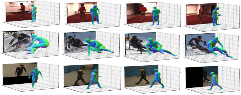
Figure 3: Visualization of reconstructed SMPL mesh for Human3.6M (row 1), SkiPose (rows 2) and TotalCapture (row 3) datasets (select four views for latter two datasets).

Qualitative results. Figure 3 gives qualitative examples where we visualize our predicted 3D mesh on images from the three testing datasets. Notably, we train only one model and test on different datasets. The results demonstrate the robustness and generalization ability of our synthetically-trained model to various unseen in-the-wild data.

Conclusion

To the best of our knowledge, we propose the first multi-view human mesh recovery method based on self-supervised synthetic training. Our solution first extracts intermediate 2D representations from each view and projects the corresponding features to a 3D canonical space with learnable volumetric calibration. Multi-stage progressive regressors then iteratively refine estimated mesh parameters based on different feature-sampling criteria. Extensive evaluations demonstrate the efficacy and superior performance of the proposed method, especially in challenging in-the-wild scenarios where 1) single-view-based methods suffer from depth ambiguities and 2) supervision-based methods have no access to any prior of in-domain image and annotation.

References

- Agarwal and Triggs (2005) Agarwal, A.; and Triggs, B. 2005. Recovering 3D human pose from monocular images. IEEE transactions on pattern analysis and machine intelligence, 28(1): 44–58.
- Arnab, Doersch, and Zisserman (2019) Arnab, A.; Doersch, C.; and Zisserman, A. 2019. Exploiting temporal context for 3D human pose estimation in the wild. In CVPR.
- Bartol et al. (2022) Bartol, K.; Bojanić, D.; Petković, T.; and Pribanić, T. 2022. Generalizable Human Pose Triangulation. In CVPR, 11028–11037.
- Bogo et al. (2016) Bogo, F.; Kanazawa, A.; Lassner, C.; Gehler, P.; Romero, J.; and Black, M. J. 2016. Keep it SMPL: Automatic estimation of 3D human pose and shape from a single image. In ECCV, 561–578. Springer.
- C (2003) C. 2003. MoCap. In mocap. cs. cmu.
- Chen and Ramanan (2017) Chen, C.-H.; and Ramanan, D. 2017. 3D Human Pose Estimation = 2D Pose Estimation + Matching. In CVPR, 5759–5767.
- Dong et al. (2019) Dong, J.; Jiang, W.; Huang, Q.; Bao, H.; and Zhou, X. 2019. Fast and Robust Multi-Person 3D Pose Estimation from Multiple Views.
- Dong et al. (2021) Dong, Z.; Song, J.; Chen, X.; Guo, C.; and Hilliges, O. 2021. Shape-aware multi-person pose estimation from multi-view images. In Proceedings of the IEEE/CVF International Conference on Computer Vision, 11158–11168.
- Gholami et al. (2021) Gholami, M.; Wandt, B.; Rhodin, H.; Ward, R.; and Wang, Z. J. 2021. AdaptPose: Cross-Dataset Adaptation for 3D Human Pose Estimation by Learnable Motion Generation. arXiv preprint arXiv:2112.11593.
- Gong et al. (2022) Gong, X.; Zheng, M.; Planche, B.; Karanam, S.; Chen, T.; Doermann, D.; and Wu, Z. 2022. Self-supervised Human Mesh Recovery with Cross-Representation Alignment. In European Conference on Computer Vision, 212–230. Springer.
- He et al. (2017) He, K.; Gkioxari, G.; Dollár, P.; and Girshick, R. 2017. Mask r-cnn. In ICCV, 2961–2969.
- Ionescu et al. (2013) Ionescu, C.; Papava, D.; Olaru, V.; and Sminchisescu, C. 2013. Human3. 6m: Large scale datasets and predictive methods for 3d human sensing in natural environments. PAMI, 36(7): 1325–1339.
- Iskakov et al. (2019) Iskakov, K.; Burkov, E.; Lempitsky, V.; and Malkov, Y. 2019. Learnable triangulation of human pose. In ICCV, 7718–7727.
- Jaderberg et al. (2015) Jaderberg, M.; Simonyan, K.; Zisserman, A.; et al. 2015. Spatial transformer networks. NeurIPS, 28.
- Kanazawa et al. (2018) Kanazawa, A.; Black, M. J.; Jacobs, D. W.; and Malik, J. 2018. End-to-end recovery of human shape and pose. In CVPR, 7122–7131.
- Kingma and Ba (2014) Kingma, D. P.; and Ba, J. 2014. Adam: A method for stochastic optimization. arXiv preprint arXiv:1412.6980.
- Kocabas, Karagoz, and Akbas (2019) Kocabas, M.; Karagoz, S.; and Akbas, E. 2019. Self-supervised learning of 3d human pose using multi-view geometry. In CVPR, 1077–1086.
- Kolotouros et al. (2019) Kolotouros, N.; Pavlakos, G.; Black, M. J.; and Daniilidis, K. 2019. Learning to reconstruct 3D human pose and shape via model-fitting in the loop. In ICCV, 2252–2261.
- Kolotouros et al. (2021) Kolotouros, N.; Pavlakos, G.; Jayaraman, D.; and Daniilidis, K. 2021. Probabilistic Modeling for Human Mesh Recovery. In ICCV.
- Kundu et al. (2020) Kundu, J. N.; Seth, S.; Jampani, V.; Rakesh, M.; Babu, R. V.; and Chakraborty, A. 2020. Self-supervised 3D human pose estimation via part guided novel image synthesis. In CVPR, 6152–6162.
- Lassner et al. (2017) Lassner, C.; Romero, J.; Kiefel, M.; Bogo, F.; Black, M. J.; and Gehler, P. V. 2017. Unite the people: Closing the loop between 3d and 2d human representations. In CVPR, 6050–6059.
- Li and Lee (2019) Li, C.; and Lee, G. H. 2019. Generating Multiple Hypotheses for 3D Human Pose Estimation With Mixture Density Network. In CVPR.
- Li et al. (2021) Li, J.; Xu, C.; Chen, Z.; Bian, S.; Yang, L.; and Lu, C. 2021. HybrIK: A Hybrid Analytical-Neural Inverse Kinematics Solution for 3D Human Pose and Shape Estimation. In CVPR.
- Li, Zhang, and Chan (2015) Li, S.; Zhang, W.; and Chan, A. B. 2015. Maximum-Margin Structured Learning with Deep Networks for 3D Human Pose Estimation. In 2015 IEEE International Conference on Computer Vision (ICCV), 2848–2856.
- Li, Oskarsson, and Heyden (2021) Li, Z.; Oskarsson, M.; and Heyden, A. 2021. 3D Human Pose and Shape Estimation Through Collaborative Learning and Multi-View Model-Fitting. In WACV, 1888–1897.
- Liang and Lin (2019) Liang, J.; and Lin, M. C. 2019. Shape-aware human pose and shape reconstruction using multi-view images. In ICCV, 4352–4362.
- Loper et al. (2015) Loper, M.; Mahmood, N.; Romero, J.; Pons-Moll, G.; and Black, M. J. 2015. SMPL: A skinned multi-person linear model. ACM transactions on graphics (TOG), 34(6): 1–16.
- Martinez et al. (2017) Martinez, J.; Hossain, R.; Romero, J.; and Little, J. J. 2017. A simple yet effective baseline for 3d human pose estimation. In ICCV.
- Mehta et al. (2017) Mehta, D.; Rhodin, H.; Casas, D.; Fua, P.; Sotnychenko, O.; Xu, W.; and Theobalt, C. 2017. Monocular 3d human pose estimation in the wild using improved cnn supervision. In 2017 international conference on 3D vision (3DV), 506–516. IEEE.
- Patel et al. (2021) Patel, P.; Huang, C.-H. P.; Tesch, J.; Hoffmann, D. T.; Tripathi, S.; and Black, M. J. 2021. AGORA: Avatars in geography optimized for regression analysis. In CVPR, 13468–13478.
- Pavlakos, Zhou, and Daniilidis (2018) Pavlakos, G.; Zhou, X.; and Daniilidis, K. 2018. Ordinal depth supervision for 3d human pose estimation. In CVPR, 7307–7316.
- Pavlakos et al. (2017a) Pavlakos, G.; Zhou, X.; Derpanis, K. G.; and Daniilidis, K. 2017a. Coarse-to-Fine Volumetric Prediction for Single-Image 3D Human Pose. In CVPR.
- Pavlakos et al. (2017b) Pavlakos, G.; Zhou, X.; Derpanis, K. G.; and Daniilidis, K. 2017b. Harvesting multiple views for marker-less 3d human pose annotations. In CVPR, 6988–6997.
- Pavlakos et al. (2018) Pavlakos, G.; Zhu, L.; Zhou, X.; and Daniilidis, K. 2018. Learning to estimate 3D human pose and shape from a single color image. In CVPR, 459–468.
- Pavllo et al. (2019) Pavllo, D.; Feichtenhofer, C.; Grangier, D.; and Auli, M. 2019. 3d human pose estimation in video with temporal convolutions and semi-supervised training. In CVPR, 7753–7762.
- Qiu et al. (2019) Qiu, H.; Wang, C.; Wang, J.; Wang, N.; and Zeng, W. 2019. Cross View Fusion for 3D Human Pose Estimation. In ICCV.
- Ravi et al. (2020) Ravi, N.; Reizenstein, J.; Novotny, D.; Gordon, T.; Lo, W.-Y.; Johnson, J.; and Gkioxari, G. 2020. Accelerating 3D Deep Learning with PyTorch3D. arXiv:2007.08501.
- Remelli et al. (2020) Remelli, E.; Han, S.; Honari, S.; Fua, P.; and Wang, R. 2020. Lightweight multi-view 3d pose estimation through camera-disentangled representation. In CVPR, 6040–6049.
- Rhodin, Salzmann, and Fua (2018) Rhodin, H.; Salzmann, M.; and Fua, P. 2018. Unsupervised geometry-aware representation for 3d human pose estimation. In ECCV, 750–767.
- Rhodin et al. (2018) Rhodin, H.; Spörri, J.; Katircioglu, I.; Constantin, V.; Meyer, F.; Müller, E.; Salzmann, M.; and Fua, P. 2018. Learning monocular 3d human pose estimation from multi-view images. In CVPR, 8437–8446.
- Rogez and Schmid (2016) Rogez, G.; and Schmid, C. 2016. MoCap-guided Data Augmentation for 3D Pose Estimation in the Wild. In NeurIPS, 3108–3116.
- Rong et al. (2019) Rong, Y.; Liu, Z.; Li, C.; Cao, K.; and Loy, C. C. 2019. Delving deep into hybrid annotations for 3d human recovery in the wild. In ICCV, 5340–5348.
- Sengupta, Budvytis, and Cipolla (2020) Sengupta, A.; Budvytis, I.; and Cipolla, R. 2020. Synthetic training for accurate 3d human pose and shape estimation in the wild. In BMVC.
- Sengupta, Budvytis, and Cipolla (2021a) Sengupta, A.; Budvytis, I.; and Cipolla, R. 2021a. Hierarchical Kinematic Probability Distributions for 3D Human Shape and Pose Estimation From Images in the Wild. In ICCV, 11219–11229.
- Sengupta, Budvytis, and Cipolla (2021b) Sengupta, A.; Budvytis, I.; and Cipolla, R. 2021b. Probabilistic 3D Human Shape and Pose Estimation From Multiple Unconstrained Images in the Wild. In CVPR, 16094–16104.
- Song et al. (2021) Song, L.; Yu, G.; Yuan, J.; and Liu, Z. 2021. Human pose estimation and its application to action recognition: A survey. Journal of Visual Communication and Image Representation, 76: 103055.
- Spörri (2016) Spörri, J. 2016. Reasearch dedicated to sports injury prevention-the’sequence of prevention’on the example of alpine ski racing. Habilitation with Venia Docendi in Biomechanics, 1(2): 7.
- Su et al. (2022) Su, J.; Wang, C.; Ma, X.; Zeng, W.; and Wang, Y. 2022. VirtualPose: Learning Generalizable 3D Human Pose Models from Virtual Data. In European Conference on Computer Vision, 55–71. Springer.
- Sun et al. (2018) Sun, X.; Xiao, B.; Liang, S.; and Wei, Y. 2018. Integral Human Pose Regression. In ECCV.
- Tan, Budvytis, and Cipolla (2017) Tan, J.; Budvytis, I.; and Cipolla, R. 2017. Indirect deep structured learning for 3D human body shape and pose prediction. In BMVC.
- Tome et al. (2018) Tome, D.; Toso, M.; Agapito, L.; and Russell, C. 2018. Rethinking pose in 3d: Multi-stage refinement and recovery for markerless motion capture. In International Conference on 3D vision (3DV), 474–483. IEEE.
- Trumble et al. (2018) Trumble, M.; Gilbert, A.; Hilton, A.; and Collomosse, J. 2018. Deep autoencoder for combined human pose estimation and body model upscaling. In ECCV, 784–800.
- Trumble et al. (2017) Trumble, M.; Gilbert, A.; Malleson, C.; Hilton, A.; and Collomosse, J. 2017. Total Capture: 3D Human Pose Estimation Fusing Video and Inertial Sensors. In BMVC.
- Varol et al. (2017) Varol, G.; Romero, J.; Martin, X.; Mahmood, N.; Black, M. J.; Laptev, I.; and Schmid, C. 2017. Learning from synthetic humans. In CVPR, 109–117.
- von Marcard et al. (2018) von Marcard, T.; Henschel, R.; Black, M. J.; Rosenhahn, B.; and Pons-Moll, G. 2018. Recovering accurate 3d human pose in the wild using imus and a moving camera. In ECCV, 601–617.
- Wandt et al. (2021) Wandt, B.; Rudolph, M.; Zell, P.; Rhodin, H.; and Rosenhahn, B. 2021. CanonPose: Self-supervised monocular 3D human pose estimation in the wild. In CVPR, 13294–13304.
- Wehrbein et al. (2021) Wehrbein, T.; Rudolph, M.; Rosenhahn, B.; and Wandt, B. 2021. Probabilistic Monocular 3D Human Pose Estimation With Normalizing Flows. In ICCV, 11199–11208.
- Wei et al. (2016) Wei, S.-E.; Ramakrishna, V.; Kanade, T.; and Sheikh, Y. 2016. Convolutional pose machines. In CVPR, 4724–4732.
- Yu et al. (2021) Yu, Z.; Wang, J.; Xu, J.; Ni, B.; Zhao, C.; Wang, M.; and Zhang, W. 2021. Skeleton2Mesh: Kinematics Prior Injected Unsupervised Human Mesh Recovery. In ICCV, 8619–8629.
- Zhang et al. (2021) Zhang, Y.; Li, Z.; An, L.; Li, M.; Yu, T.; and Liu, Y. 2021. Lightweight multi-person total motion capture using sparse multi-view cameras. In Proceedings of the IEEE/CVF International Conference on Computer Vision, 5560–5569.
- Zheng et al. (2022) Zheng, M.; Planche, B.; Gong, X.; Yang, F.; Chen, T.; and Wu, Z. 2022. Self-supervised 3d patient modeling with multi-modal attentive fusion. In International Conference on Medical Image Computing and Computer-Assisted Intervention, 115–125. Springer.
- Zheng et al. (2019) Zheng, Z.; Yu, T.; Wei, Y.; Dai, Q.; and Liu, Y. 2019. Deephuman: 3d human reconstruction from a single image. In ICCV, 7739–7749.
- Zhou et al. (2019a) Zhou, K.; Han, X.; Jiang, N.; Jia, K.; and Lu, J. 2019a. HEMlets Pose: Learning Part-Centric Heatmap Triplets for Accurate 3D Human Pose Estimation. In ICCV.
- Zhou et al. (2019b) Zhou, Y.; Barnes, C.; Lu, J.; Yang, J.; and Li, H. 2019b. On the continuity of rotation representations in neural networks. In CVPR, 5745–5753.
- Zhu, Karlsson, and Bregler (2020) Zhu, T.; Karlsson, P.; and Bregler, C. 2020. Simpose: Effectively learning densepose and surface normals of people from simulated data. In ECCV, 225–242. Springer.