The entropy production of stationary diffusions

Lancelot Da Costa1,2,12{}^{1,2,}\thanks{Correspondence: \url{l.da-costa@imperial.ac.uk}}\> & Grigorios A. Pavliotis1

1Department of Mathematics, Imperial College London
2Wellcome Centre for Human Neuroimaging, University College London
Correspondence: l.da-costa@imperial.ac.uk
Abstract

The entropy production rate is a central quantity in non-equilibrium statistical physics, scoring how far a stochastic process is from being time-reversible. In this paper, we compute the entropy production of diffusion processes at non-equilibrium steady-state under the condition that the time-reversal of the diffusion remains a diffusion. We start by characterising the entropy production of both discrete and continuous-time Markov processes. We investigate the time-reversal of time-homogeneous stationary diffusions and recall the most general conditions for the reversibility of the diffusion property, which includes hypoelliptic and degenerate diffusions, and locally Lipschitz vector fields. We decompose the drift into its time-reversible and irreversible parts, or equivalently, the generator into symmetric and antisymmetric operators. We show the equivalence with a decomposition of the backward Kolmogorov equation considered in hypocoercivity theory, and a decomposition of the Fokker-Planck equation in GENERIC form. The main result shows that when the time-irreversible part of the drift is in the range of the volatility matrix (almost everywhere) the forward and time-reversed path space measures of the process are mutually equivalent, and evaluates the entropy production. When this does not hold, the measures are mutually singular and the entropy production is infinite. We verify these results using exact numerical simulations of linear diffusions. We illustrate the discrepancy between the entropy production of non-linear diffusions and their numerical simulations in several examples and illustrate how the entropy production can be used for accurate numerical simulation. Finally, we discuss the relationship between time-irreversibility and sampling efficiency, and how we can modify the definition of entropy production to score how far a process is from being generalised reversible.

Keywords: measuring irreversibility; time-reversal; hypoelliptic; degenerate diffusion; Helmholtz decomposition; numerical simulation; Langevin equation; stochastic differential equation; entropy production rate.

1 Introduction

The entropy production rate epsubscript𝑒𝑝e_{p} is a central concept in statistical physics. In a nutshell, it is a measure of the time-irreversibility of a stochastic process, that is how much random motion differs statistically speaking as one plays it forward, or backward, in time.

At non-equilibrium steady-state, the epsubscript𝑒𝑝e_{p} is quantified by the relative entropy HH\operatorname{H} (a.k.a Kullback-Leibler divergence)

ep=1TH[𝐏[0,T]𝐏¯[0,T]]subscript𝑒𝑝1𝑇Hconditionalsubscript𝐏0𝑇subscript¯𝐏0𝑇\displaystyle e_{p}=\frac{1}{T}\operatorname{H}[\mathbf{P}_{[0,T]}\mid\bar{\mathbf{P}}_{[0,T]}]

between the path-wise distributions of the forward and time-reversed processes in some time interval [0,T]0𝑇[0,T], denoted by 𝐏[0,T],𝐏¯[0,T]subscript𝐏0𝑇subscript¯𝐏0𝑇\mathbf{P}_{[0,T]},\bar{\mathbf{P}}_{[0,T]}, respectively.

Physically, the epsubscript𝑒𝑝e_{p} measures the minimal amount of energy needed, per unit of time, to maintain a system at non-equilibrium steady-state. Equivalently, it quantifies the heat dissipated by a physical system at non-equilibrium steady-state per unit of time [1, p. 86]. The second law of thermodynamics for open systems is the non-negativity of the entropy production.

The epsubscript𝑒𝑝e_{p} plays a crucial role in stochastic thermodynamics. It is the central quantity in the so-called Gallavotti-Cohen fluctuation theorem, which quantifies the probability of entropy decrease along stochastic trajectories [2, 3, 4]. More recently, entropy production is at the heart of the so-called thermodynamic uncertainty relations, which provide estimates of epsubscript𝑒𝑝e_{p} from observations of the system [5]. The epsubscript𝑒𝑝e_{p} is also an important tool in biophysics, as a measure of the metabolic cost of molecular processes, such as molecular motors [2], and it was shown empirically that brain states associated with effortful activity correlated with a higher entropy production from neural activity [6].

In this paper, we will be primarily concerned with the entropy production of diffusion processes, that is, solutions of stochastic differential equations. Consider an Itô stochastic differential equation (SDE)

dxt=b(xt)dt+σ(xt)dwtdsubscript𝑥𝑡𝑏subscript𝑥𝑡d𝑡𝜎subscript𝑥𝑡dsubscript𝑤𝑡\mathrm{d}x_{t}=b\left(x_{t}\right)\mathrm{d}t+\sigma\left(x_{t}\right)\mathrm{d}w_{t}

with drift b:dd:𝑏superscript𝑑superscript𝑑b:\mathbb{R}^{d}\to\mathbb{R}^{d} and volatility σ:dd×m:𝜎superscript𝑑superscript𝑑𝑚\sigma:\mathbb{R}^{d}\to\mathbb{R}^{d\times m}, and wtsubscript𝑤𝑡w_{t} a standard Brownian motion on msuperscript𝑚\mathbb{R}^{m}, whose solution is stationary at a probability measure μ𝜇\mu with density ρ𝜌\rho. A result known as the Helmholtz decomposition, which is central in non-equilibrium statistical physics [7, 8, 9, 10] but also in statistical sampling [11, 12, 13, 14], tells us that we can decompose the drift into time-reversible and time-irreversible parts: b=brev+birr𝑏subscript𝑏revsubscript𝑏irrb=b_{\mathrm{rev}}+b_{\mathrm{irr}}. In particular, birrρsubscript𝑏irr𝜌b_{\mathrm{irr}}\rho is the stationary probability current, as considered by Nelson [15]. Jiang and colleagues derived the entropy production rate for such systems under the constraint that the coefficients of the SDE b,σ𝑏𝜎b,\sigma are globally Lipschitz, and the solution uniformly elliptic (i.e., the diffusion matrix field D=12σσ𝐷12𝜎superscript𝜎topD=\frac{1}{2}\sigma\sigma^{\top} is uniformly positive definite). This takes the form of [1, Chapter 4]:

ep=dbirrD1birrρ(x)dx.subscript𝑒𝑝subscriptsuperscript𝑑superscriptsubscript𝑏irrtopsuperscript𝐷1subscript𝑏irr𝜌𝑥differential-d𝑥\displaystyle e_{p}=\int_{\mathbb{R}^{d}}b_{\mathrm{irr}}^{\top}D^{-1}b_{\mathrm{irr}}\rho(x)\mathrm{d}x.

In this paper, we extend their work by computing the entropy production for a greater range of diffusion processes, which includes non-elliptic, hypoelliptic and degenerate diffusions, and SDEs driven by locally Lipschitz coefficients. Non-elliptic diffusions are solutions to SDEs whose diffusion matrix field D=12σσ𝐷12𝜎superscript𝜎topD=\frac{1}{2}\sigma\sigma^{\top} is not positive definite everywhere; this means that there are regions of space in which the random fluctuations cannot drive the process in every possible direction. Depending on how the volatility interacts with the drift (i.e., Hörmander’s theorem [16, Theorem 1.3]), solutions initialised at a point may still have a density—the hypoelliptic case—or not—the degenerate case; prominent examples are underdamped Langevin dynamics and deterministic dynamics, respectively. In our treatment, we only assume that the time-reversal of a diffusion is a diffusion (the necessary and sufficient conditions for which were first established by Millet, Nualart and Sanz [17]) and sufficient regularity to apply Girsanov’s theorem or the Stroock-Varadhan support theorem.

This extension has become important since many processes that are commonplace in non-equilibrium statistical physics or statistical machine learning are hypoelliptic. For instance, the underdamped and generalised Langevin equations in phase space [10], which model the motion of a particle interacting with a heat bath, and which form the basis of efficient sampling schemes such as Hamiltonian Monte-Carlo [13], or, stochastic gradient descent in deep neural networks [14], or, the linear diffusion process with the fastest convergence to stationary state [18], which informs us of the properties of efficient samplers. Much research in statistical sampling has drawn the connection between time-irreversibility and sampling efficiency [19, 13, 20, 21], so it is informative to understand the amount of time-irreversibility associated with the most efficient samplers. Lastly, it is known that numerically integrating a diffusion processes can modify the amount of irreversibility present in the original dynamic [22]. The entropy production rate is thus an important indicator of the fidelity of a numerical simulation, and can serve as a guide to developing sampling schemes that preserve the statistical properties of efficient (hypoelliptic) samplers.

The outline of the paper and our contribution are detailed below.

1.1 Paper outline and contribution

Section 2:

We give various characterisations and formulas for the epsubscript𝑒𝑝e_{p} of stationary Markov processes in discrete and continuous-time, and recall a crude but general recipe for numerical estimation.

Section 3:

We investigate the time-reversal of time-homogeneous diffusions. We give the general conditions under which the time-reversal of a time-homogeneous diffusion remains a diffusion, based on the results of Millet, Nualart and Sanz [17]. We then recall how the drift vector field of an SDE can be decomposed into time-reversible and irreversible parts. We show that this decomposition is equivalent to a decomposition of the generator of the process into symmetric and antisymmetric operators on a suitable function space. Then we show that this decomposition is equivalent to two other fundamental decompositions in the study of far from equilibrium systems: the decomposition of the backward Kolmogorov equation considered in hypocoercivity theory [23, 24] and the decomposition of the Fokker-Planck equation considered in the GENERIC formalism [23, 25].

Section 4:

We compute the epsubscript𝑒𝑝e_{p} of stationary diffusion processes under the condition that the time-reversal of the diffusion remains a diffusion. We show that:

  • Section 4.1: If birr(x)Rangeσ(x)subscript𝑏irr𝑥Range𝜎𝑥b_{\mathrm{irr}}(x)\in\operatorname{Range}\sigma(x), for μ𝜇\mu-almost every xd𝑥superscript𝑑x\in\mathbb{R}^{d}111μ𝜇\mu-almost everywhere: This means that the statement holds with probability 111 when x𝑥x is distributed according to the probability measure μ𝜇\mu. (in particular for elliptic or time-reversible diffusions). Then the forward and backward path-space measures are mutually equivalent, in other words, the sets of possible trajectories by forward and backward processes are equal—and the entropy production equals ep=birrDbirrdμsubscript𝑒𝑝superscriptsubscript𝑏irrtopsuperscript𝐷subscript𝑏irrdifferential-d𝜇e_{p}=\int b_{\mathrm{irr}}^{\top}D^{-}b_{\mathrm{irr}}\mathrm{d}\mu, where superscript\cdot^{-} denotes the Moore-Penrose matrix pseudo-inverse. See Theorems 4.1, 4.2 for details.

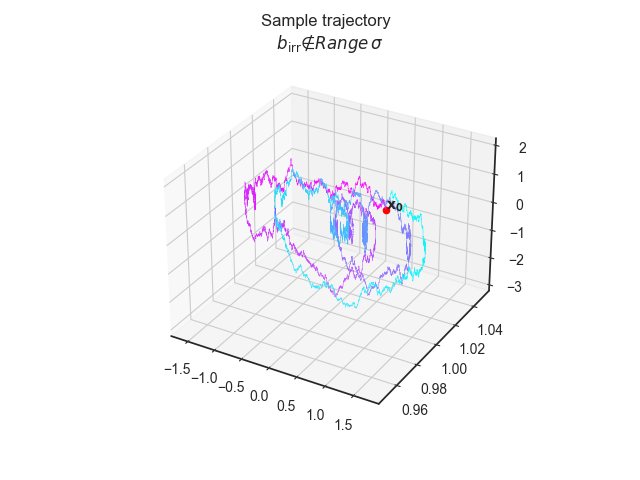
  • Section 4.2: When the above does not hold, the forward and backward path-space measures are mutually singular, in other words, there are trajectories that are taken by the forward process that cannot be taken by the backward process—and vice-versa222Precisely, two measures are mutual singular if and only if they are not mutually equivalent.. In particular, the entropy production rate is infinite ep=+subscript𝑒𝑝e_{p}=+\infty. See Theorem 4.4 for details.

Section 5:

We compute the epsubscript𝑒𝑝e_{p} of various models such as the multivariate Ornstein-Uhlenbeck and the underdamped Langevin process. We numerically simulate and verify the value of epsubscript𝑒𝑝e_{p} when the coefficients are linear. We then discuss how numerical discretisation can influence the value of epsubscript𝑒𝑝e_{p}. As examples, we compute and compare the epsubscript𝑒𝑝e_{p} of Euler-Maruyama and BBK [26, 27] discretisations of the underdamped Langevin process. We summarise the usefulness of epsubscript𝑒𝑝e_{p} as a measure of the accuracy of numerical schemes in preserving the time-irreversibility properties of the underlying process, and give guidelines, in terms of epsubscript𝑒𝑝e_{p}, for developing accurate simulations of underdamped Langevin dynamics.

Section 6:

We give a geometric interpretation of our main results and discuss future perspectives: what this suggests about the relationship between time-irreversibility and mixing in the context of sampling and optimisation, and how we could modify the definition—and computation—of epsubscript𝑒𝑝e_{p} to quantify how a process is far from being time-reversible up to a one-to-one transformation of its phase-space.

2 The epsubscript𝑒𝑝e_{p} of stationary Markov processes

In this section, (xt)t[0,T],T>0subscriptsubscript𝑥𝑡𝑡0𝑇𝑇0(x_{t})_{t\in[0,T]},T>0 is a time-homogeneous Markov process on a Polish space 𝒳𝒳\mathcal{X} with almost surely (a.s.) continuous trajectories.

Definition 2.1 (Time reversed process).

The time reversed process (x¯t)t[0,T]subscriptsubscript¯𝑥𝑡𝑡0𝑇(\bar{x}_{t})_{t\in[0,T]} is defined as x¯t=xTtsubscript¯𝑥𝑡subscript𝑥𝑇𝑡\bar{x}_{t}=x_{T-t}.

Note that since the final state of the forward process is the initial state of the backward process this definition makes sense only on finite time intervals.

We define (C([0,T],𝒳),d)𝐶0𝑇𝒳subscript𝑑\left(C([0,T],\mathcal{X}),d_{\infty}\right) as the space of 𝒳𝒳\mathcal{X}-valued continuous paths endowed with the supremum distance dsubscript𝑑d_{\infty}, defined as d(f,g)=supt[0,T]d(f(t),g(t))subscript𝑑𝑓𝑔subscriptsupremum𝑡0𝑇𝑑𝑓𝑡𝑔𝑡d_{\infty}(f,g)=\sup_{t\in[0,T]}d(f(t),g(t)), where d𝑑d is a choice of distance on the Polish space 𝒳𝒳\mathcal{X}. Naturally, when we later specialise to 𝒳=d𝒳superscript𝑑\mathcal{X}=\mathbb{R}^{d}, the supremum distance will be given by the Lsuperscript𝐿L^{\infty}-norm \|\cdot\|_{\infty}.

Definition 2.2 (Path space measure).

Each Markov process (xt)0tTsubscriptsubscript𝑥𝑡0𝑡𝑇(x_{t})_{0\leq t\leq T} with a.s. continuous trajectories defines probability measure 𝐏[0,T]subscript𝐏0𝑇\mathbf{P}_{[0,T]} on the canonical path space (C([0,T],𝒳),)𝐶0𝑇𝒳\left(C([0,T],\mathcal{X}),\mathscr{B}\right), where \mathscr{B} is the Borel sigma-algebra associated with the supremum distance. This probability measure determines the probability of the process to take any (Borel set of) paths.

Remark 2.3 (Cadlag Markov processes).

All definitions and results in this section hold more generally for Markov processes with cadlag paths (i.e., right continuous with left limits), simply replacing the canonical path-space (C([0,T],𝒳),d)𝐶0𝑇𝒳subscript𝑑\left(C([0,T],\mathcal{X}),d_{\infty}\right) with the Skorokhod space. We restrict ourselves to processes with continuous paths for simplicity.

Definition 2.4 (Restriction to a sub-interval of time).

Given a path space measure 𝐏[0,T]subscript𝐏0𝑇\mathbf{P}_{[0,T]} and times a<b[0,T]𝑎𝑏0𝑇a<b\in[0,T], we define 𝐏[a,b]subscript𝐏𝑎𝑏\mathbf{P}_{[a,b]} to be the path space measure describing (xt)t[a,b]subscriptsubscript𝑥𝑡𝑡𝑎𝑏\left(x_{t}\right)_{t\in[a,b]}. This is the restriction of 𝐏[0,T]subscript𝐏0𝑇\mathbf{P}_{[0,T]} to the sub sigma-algebra [a,b]:={A:A|[a,b]Borel sigma-algebra on(C([a,b],𝒳),d)}assignsubscript𝑎𝑏conditional-set𝐴evaluated-at𝐴𝑎𝑏Borel sigma-algebra on𝐶𝑎𝑏𝒳subscript𝑑\mathscr{B}_{[a,b]}:=\left\{A\in\mathscr{B}:\left.A\right|_{[a,b]}\in\text{Borel sigma-algebra on}\left(C([a,b],\mathcal{X}),d_{\infty}\right)\right\}.

Let 𝐏𝐏\mathbf{P} be the path space measure of the Markov process xtsubscript𝑥𝑡x_{t} and 𝐏¯¯𝐏\bar{\mathbf{P}} be that of its time-reversal x¯tsubscript¯𝑥𝑡\bar{x}_{t}, respectively. We can measure the statistical difference between the forward and time-reversed processes at time τ[0,T]𝜏0𝑇\tau\in[0,T] with the entropy production rate

limε01εH[𝐏[τ,τ+ε],𝐏¯[τ,τ+ε]],subscript𝜀01𝜀Hsubscript𝐏𝜏𝜏𝜀subscript¯𝐏𝜏𝜏𝜀\displaystyle\lim_{\varepsilon\downarrow 0}\frac{1}{\varepsilon}\operatorname{H}\left[\mathbf{P}_{[\tau,\tau+\varepsilon]},\bar{\mathbf{P}}_{[\tau,\tau+\varepsilon]}\right], (1)

where HH\operatorname{H} is the relative entropy (a.k.a. Kullback-Leibler divergence). This measures the rate at which the forward and backward path space measures differ in the relative entropy sense at time τ𝜏\tau.

The following result [1, Theorem 2.2.4] (see also [28, Theorem 10.4]) shows that the limit exists in stationary and time-homogeneous Markov processes. Obviously, the limit is independent of τ𝜏\tau in this case.

Theorem 2.5.

Suppose that (xt)t[0,T]subscriptsubscript𝑥𝑡𝑡0𝑇\left(x_{t}\right)_{t\in[0,T]} is a stationary time-homogeneous Markov process on a Polish space 𝒳𝒳\mathcal{X} with continuous sample paths. Stationarity implies that we can set the time-horizon T>0𝑇0T>0 of the process to arbitrarily large values. Then the quantity

1tH[𝐏[τ,τ+t]𝐏¯[τ,τ+t]] for all τ[0,+),t(0,+)formulae-sequence1𝑡Hconditionalsubscript𝐏𝜏𝜏𝑡subscript¯𝐏𝜏𝜏𝑡 for all 𝜏0𝑡0\displaystyle\frac{1}{t}\operatorname{H}\left[\mathbf{P}_{[\tau,\tau+t]}\mid\bar{\mathbf{P}}_{[\tau,\tau+t]}\right]\text{ for all }\tau\in[0,+\infty),t\in(0,+\infty)

is a constant [0,+]absent0\in[0,+\infty].

This yields the following general definition of entropy production rate for stationary Markov processes:

Definition 2.6 (Entropy production rate of a stationary Markov process).

Let (xt)t[0,T]subscriptsubscript𝑥𝑡𝑡0𝑇\left(x_{t}\right)_{t\in[0,T]} be a stationary time-homogeneous Markov process. Stationarity implies that we can set the time-horizon T>0𝑇0T>0 to be arbitrarily large. For such processes, the entropy production rate is a constant ep[0,+]subscript𝑒𝑝0e_{p}\in[0,+\infty] defined as

ep:=1tH[𝐏[0,t]𝐏¯[0,t]]assignsubscript𝑒𝑝1𝑡Hconditionalsubscript𝐏0𝑡subscript¯𝐏0𝑡e_{p}:=\frac{1}{t}\operatorname{H}\left[\mathbf{P}_{[0,t]}\mid\bar{\mathbf{P}}_{[0,t]}\right] (2)

for any t(0,+)𝑡0t\in(0,+\infty). epsubscript𝑒𝑝e_{p} scores the amount to which the forward and time-reversed processes differ per unit of time. In particular, Tep𝑇subscript𝑒𝑝Te_{p} is the total entropy production in a time interval of length T𝑇T. Note that, in the literature, the epsubscript𝑒𝑝e_{p} is often defined as ep=limt+1tH[𝐏[0,t]𝐏¯[0,t]]subscript𝑒𝑝subscript𝑡1𝑡Hconditionalsubscript𝐏0𝑡subscript¯𝐏0𝑡e_{p}=\lim_{t\to+\infty}\frac{1}{t}\operatorname{H}\left[\mathbf{P}_{[0,t]}\mid\bar{\mathbf{P}}_{[0,t]}\right], e.g., [1, Definition 4.1.1]; this is just (2) in the limit of large t𝑡t. However, Theorem 2.5 showed us that (2) is constant w.r.t. t(0,+)𝑡0t\in(0,+\infty) so we do not need to restrict ourselves to defining the epsubscript𝑒𝑝e_{p} as (2) in the limit of large t𝑡t. This added generality will be very helpful to compute epsubscript𝑒𝑝e_{p} later, by exploiting the fact that (2) is often more easily analysed in the regime of finite or small t𝑡t.

Remark 2.7 (Physical relevance of Definition 2.6).

In some stationary processes (e.g., Hamiltonian systems), physicists define entropy production as Definition 2.6 with an additional operator applied to the path space measure of the time-reversed process; that is,

epgen,θ:=limε01εH[𝐏[0,ε],θ#𝐏¯[0,ε]],assignsuperscriptsubscript𝑒𝑝gen𝜃subscript𝜀01𝜀Hsubscript𝐏0𝜀subscript𝜃#subscript¯𝐏0𝜀e_{p}^{\mathrm{gen},\theta}:=\lim_{\varepsilon\downarrow 0}\frac{1}{\varepsilon}\operatorname{H}\left[\mathbf{P}_{[0,\varepsilon]},\theta_{\#}\bar{\mathbf{P}}_{[0,\varepsilon]}\right], (3)

where θ#subscript𝜃#\theta_{\#} is the pushforward operator associated to an involution of phase-space θ𝜃\theta (e.g., the momentum flip [29, 30, 31]) that leaves the stationary distribution invariant333This generalised definition of entropy production is taken as a limit of ε0𝜀0\varepsilon\downarrow 0 analogously to (1) to capture the fact that we are modelling a rate. We cannot, a priori state that the expression is constant for any ε(0,+)𝜀0\varepsilon\in(0,+\infty), as in Definition 2.6, since we do not know whether a result analogous to Theorem 2.5 holds in this case.. In this article, we will refer to (2) as entropy production and to (3) as generalised entropy production, and proceed to derive general results for (2). The results we derive are informative of the process and applicable independently of whether (2) is the physically meaningful definition of entropy production; yet, physicists looking to interpret these results should bear in mind that they are physically informative about entropy production insofar as Definition 2.6 is physically meaningful for the system at hand. We will briefly revisit generalised entropy production in the discussion (Section 6.2).

Proposition 2.8.

Let (xt)t[0,T]subscriptsubscript𝑥𝑡𝑡0𝑇\left(x_{t}\right)_{t\in[0,T]} be a time-homogeneous Markov process on a Polish space 𝒳𝒳\mathcal{X}, stationary at the probability measure μ𝜇\mu. Then the entropy production rate equals

ep=1t𝔼xμ[H[𝐏[0,t]x𝐏¯[0,t]x]]subscript𝑒𝑝1𝑡subscript𝔼similar-to𝑥𝜇delimited-[]Hconditionalsubscriptsuperscript𝐏𝑥0𝑡subscriptsuperscript¯𝐏𝑥0𝑡e_{p}=\frac{1}{t}\mathbb{E}_{x\sim\mu}\left[\operatorname{H}\left[\mathbf{P}^{x}_{[0,t]}\mid\bar{\mathbf{P}}^{x}_{[0,t]}\right]\right]

for any t(0,+)𝑡0t\in(0,+\infty).

A proof is provided in Appendix A.1.1.

Notation 2.9.

By 𝐏xsuperscript𝐏𝑥\mathbf{P}^{x} we mean the path space measure of the process initialised (possibly out of stationarity) at a deterministic initial condition x0=x𝒳subscript𝑥0𝑥𝒳x_{0}=x\in\mathcal{X}.

Proposition 2.10 (epsubscript𝑒𝑝e_{p} in terms of transition kernels).

Let (xt)t[0,T]subscriptsubscript𝑥𝑡𝑡0𝑇\left(x_{t}\right)_{t\in[0,T]} be a time-homogeneous Markov process on a Polish space 𝒳𝒳\mathcal{X}, stationary at the probability measure μ𝜇\mu. Denote by pt(dy,x)subscript𝑝𝑡𝑑𝑦𝑥p_{t}(dy,x) the transition kernels of the Markov semigroup, and by p¯t(dy,x)subscript¯𝑝𝑡𝑑𝑦𝑥\bar{p}_{t}(dy,x) those of the time-reversed process. Then the entropy production rate equals

ep=limε01ε𝔼xμ[H[pε(,x)p¯ε(,x)]].subscript𝑒𝑝subscript𝜀01𝜀subscript𝔼similar-to𝑥𝜇delimited-[]Hconditionalsubscript𝑝𝜀𝑥subscript¯𝑝𝜀𝑥e_{p}=\lim_{\varepsilon\downarrow 0}\frac{1}{\varepsilon}\mathbb{E}_{x\sim\mu}\left[\operatorname{H}\left[p_{\varepsilon}(\cdot,x)\mid\bar{p}_{\varepsilon}(\cdot,x)\right]\right].

The fact that the time-reversed process possesses transition kernels holds as it is also a stationary Markov process [1, p. 113]. A proof of Proposition 2.10 is provided in Appendix A.1.2.

2.1 The epsubscript𝑒𝑝e_{p} of numerical simulations

Proposition 2.10 entails a formula for the epsubscript𝑒𝑝e_{p} of Markov processes in discrete time:

Definition 2.11.

The entropy production rate of a discrete-time Markov process with time-step ε𝜀\varepsilon equals

epNS(ε)=1ε𝔼xμ~pε(y,x)logpε(y,x)pε(x,y)dy,superscriptsubscript𝑒𝑝NS𝜀1𝜀subscript𝔼similar-to𝑥~𝜇subscript𝑝𝜀𝑦𝑥subscript𝑝𝜀𝑦𝑥subscript𝑝𝜀𝑥𝑦d𝑦e_{p}^{\text{NS}}(\varepsilon)=\frac{1}{\varepsilon}\mathbb{E}_{x\sim\tilde{\mu}}\int p_{\varepsilon}(y,x)\log\frac{p_{\varepsilon}(y,x)}{p_{\varepsilon}(x,y)}\mathrm{d}y, (4)

where μ~~𝜇\tilde{\mu} is the invariant measure of the process.

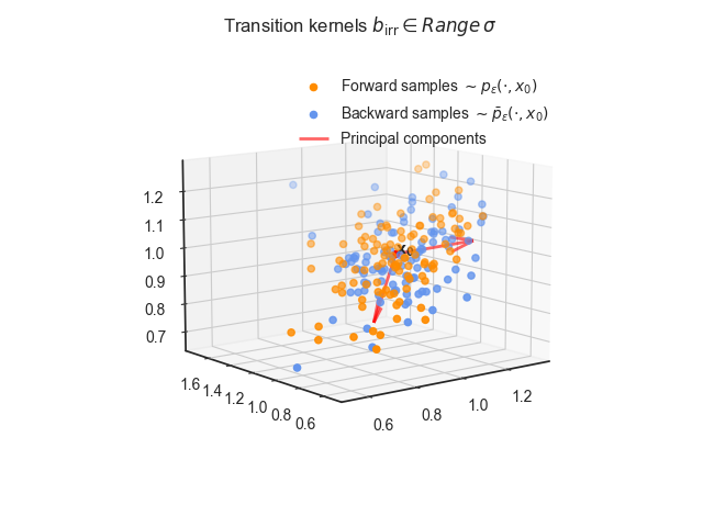
This definition is useful, for example, to quantify the entropy production of numerical simulations of a stochastic process [22]. In particular, it suggests a simple numerical estimator of the entropy production rate for numerical simulations (at stationarity). Consider a small δ𝛿\delta (e.g., δ𝛿\delta is the time-step of the numerical discretisation). Given samples from the process at δ𝛿\delta time intervals, discretise the state-space into a finite partition U1,,Unsubscript𝑈1subscript𝑈𝑛U_{1},\ldots,U_{n}, and approximate 𝐏[0,δ]subscript𝐏0𝛿\mathbf{P}_{[0,\delta]} and 𝐏¯[0,δ]subscript¯𝐏0𝛿\bar{\mathbf{P}}_{[0,\delta]} by the empirical transition probabilities pijsubscript𝑝𝑖𝑗p_{i\to j} between Ui,Ujsubscript𝑈𝑖subscript𝑈𝑗U_{i},U_{j} from time 00 to δ𝛿\delta.

epNS=limε01εH[𝐏[0,ε]𝐏¯[0,ε]]1δH[𝐏[0,δ]𝐏¯[0,δ]]1δi,jpijlogpijpji.superscriptsubscript𝑒𝑝NSsubscript𝜀01𝜀Hconditionalsubscript𝐏0𝜀subscript¯𝐏0𝜀1𝛿Hconditionalsubscript𝐏0𝛿subscript¯𝐏0𝛿1𝛿subscript𝑖𝑗subscript𝑝𝑖𝑗subscript𝑝𝑖𝑗subscript𝑝𝑗𝑖\displaystyle e_{p}^{\text{NS}}=\lim_{\varepsilon\to 0}\frac{1}{\varepsilon}\operatorname{H}\left[\mathbf{P}_{[0,\varepsilon]}\mid\bar{\mathbf{P}}_{[0,\varepsilon]}\right]\approx\frac{1}{\delta}\operatorname{H}\left[\mathbf{P}_{[0,\delta]}\mid\bar{\mathbf{P}}_{[0,\delta]}\right]\approx\frac{1}{\delta}\sum_{i,j}p_{i\to j}\log\frac{p_{i\to j}}{p_{j\to i}}.

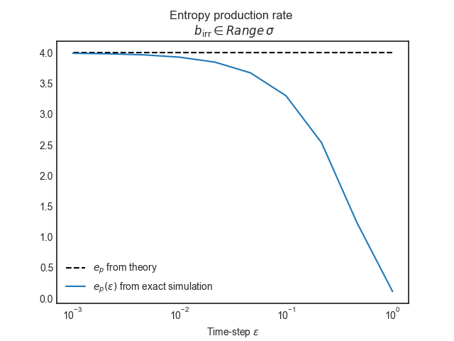
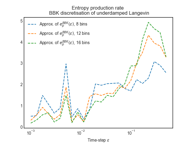
Note that this method measures the entropy production rate of the numerical discretisation as opposed to that of the continuous process. This typically produces results close to epsubscript𝑒𝑝e_{p}, but does not necessarily converge to epsubscript𝑒𝑝e_{p} in the continuum limit δ0𝛿0\delta\to 0 of the numerical discretisation. Indeed [22] showed that numerical discretisations can break detailed balance, so that the continuum limit of the numerical discretisation can differ from the initial process. Thus one should choose numerical schemes carefully when preserving the entropy production rate of a process is important. We will return to this in Section 5.

3 Time reversal of stationary diffusions

We now specialise to diffusion processes in dsuperscript𝑑\mathbb{R}^{d}. These are Markov processes with an infinitessimal generator that is a second order linear operator without a constant part [32, Definition 1.11.1], which entails almost surely (a.s.) continuous sample paths. Conveniently, diffusion processes are usually expressible as solutions to stochastic differential equations. From now on, we consider an Itô stochastic differential equation

dxt=b(xt)dt+σ(xt)dwtdsubscript𝑥𝑡𝑏subscript𝑥𝑡d𝑡𝜎subscript𝑥𝑡dsubscript𝑤𝑡\mathrm{d}x_{t}=b\left(x_{t}\right)\mathrm{d}t+\sigma\left(x_{t}\right)\mathrm{d}w_{t} (5)

with drift b:dd:𝑏superscript𝑑superscript𝑑b:\mathbb{R}^{d}\rightarrow\mathbb{R}^{d} and volatility σ:dd×m:𝜎superscript𝑑superscript𝑑𝑚\sigma:\mathbb{R}^{d}\rightarrow\mathbb{R}^{d\times m}, and wtsubscript𝑤𝑡w_{t} a standard Brownian motion on msuperscript𝑚\mathbb{R}^{m}.

Notation 3.1.

Let D=σσ/2d×d𝐷𝜎superscript𝜎top2superscript𝑑𝑑D=\sigma\sigma^{\top}/2\in\mathbb{R}^{{d\times d}} be the diffusion tensor. Denote by \|\cdot\| the Euclidean distance, and, for matrices

σ2:=i=1dj=1n|σij|2.assignsuperscriptnorm𝜎2superscriptsubscript𝑖1𝑑superscriptsubscript𝑗1𝑛superscriptsubscript𝜎𝑖𝑗2\|\sigma\|^{2}:=\sum_{i=1}^{d}\sum_{j=1}^{n}\left|\sigma_{ij}\right|^{2}.

Throughout, \nabla and \nabla\cdot are the gradient and the divergence in the distributional sense. We operationally define the divergence of a matrix field Q:dd×d:𝑄superscript𝑑superscript𝑑𝑑Q:\mathbb{R}^{d}\to\mathbb{R}^{{d\times d}} by (Q)i:=j=1djQijassignsubscript𝑄𝑖superscriptsubscript𝑗1𝑑subscript𝑗subscript𝑄𝑖𝑗(\nabla\cdot Q)_{i}:=\sum_{j=1}^{d}\partial_{j}Q_{ij} for 0id0𝑖𝑑0\leq i\leq d. We will denote by μ𝜇\mu the stationary probability measure of the process xtsubscript𝑥𝑡x_{t} and by ρ𝜌\rho its density with respect to the Lebesgue measure, i.e., μ(dx)=ρ(x)dx𝜇d𝑥𝜌𝑥d𝑥\mu(\mathrm{d}x)=\rho(x)\mathrm{d}x (assuming they exist).

3.1 On the time-reversibility of the diffusion property

There is a substantial literature studying the time-reversal of diffusion processes. In general, the time-reversal of a diffusion need not be a diffusion [17], but Haussman and Pardoux showed that the diffusion property is preserved under some mild regularity conditions on the diffusion process [33]. A few years later Millet, Nualart, Sanz derived necessary and sufficient conditions for the time-reversal of a diffusion to be a diffusion [17, Theorem 2.2 & p. 220]. We provide these conditions here, with a proof of a different nature that exploits the existence of a stationary distribution.

Lemma 3.2 (Conditions for the reversibility of the diffusion property).

Let an Itô SDE (5) with locally bounded, Lebesgue measurable coefficients b:dd,σ:dd×m:𝑏superscript𝑑superscript𝑑𝜎:superscript𝑑superscript𝑑𝑚b:\mathbb{R}^{d}\rightarrow\mathbb{R}^{d},\sigma:\mathbb{R}^{d}\rightarrow\mathbb{R}^{d\times m}. Consider a strong solution (xt)t[0,T]subscriptsubscript𝑥𝑡𝑡0𝑇(x_{t})_{t\in[0,T]}, i.e., a process satisfying

xt=x0+0tb(xs)𝑑s+0tσ(xs)𝑑ws,subscript𝑥𝑡subscript𝑥0superscriptsubscript0𝑡𝑏subscript𝑥𝑠differential-d𝑠superscriptsubscript0𝑡𝜎subscript𝑥𝑠differential-dsubscript𝑤𝑠\displaystyle x_{t}=x_{0}+\int_{0}^{t}b\left(x_{s}\right)ds+\int_{0}^{t}\sigma\left(x_{s}\right)dw_{s},

and assume that it is stationary with respect to a probability measure μ𝜇\mu with density ρ𝜌\rho. Consider the time-reversed stationary process (x¯t)t[0,T]subscriptsubscript¯𝑥𝑡𝑡0𝑇(\bar{x}_{t})_{t\in[0,T]}. Then, the following are equivalent:

  • (x¯t)t[0,T]subscriptsubscript¯𝑥𝑡𝑡0𝑇(\bar{x}_{t})_{t\in[0,T]} is a Markov diffusion process.

  • The distributional derivative (Dρ)𝐷𝜌\nabla\cdot(D\rho) is a function, which is then necessarily in Lloc1(d,d)subscriptsuperscript𝐿1locsuperscript𝑑superscript𝑑L^{1}_{\mathrm{loc}}(\mathbb{R}^{d},\mathbb{R}^{d}).

A proof is provided in Appendix A.2.1.

3.2 Setup for the time-reversal of diffusions

From now on, we will work under the assumption that the time-reversal of the diffusion is a diffusion. We assume that:

Assumption 3.3.
  1. 1.

    The coefficients of the SDE (5) b,σ𝑏𝜎b,\sigma are locally Lipschitz continuous. In other words, xd,r>0,k>0 s.t. yd::formulae-sequencefor-all𝑥superscript𝑑formulae-sequence𝑟0𝑘0 s.t. for-all𝑦superscript𝑑absent\forall x\in\mathbb{R}^{d},\exists r>0,k>0\text{ s.t. }\forall y\in\mathbb{R}^{d}:

    xy<rb(x)b(y)+σ(x)σ(y)kxy,norm𝑥𝑦𝑟norm𝑏𝑥𝑏𝑦norm𝜎𝑥𝜎𝑦𝑘norm𝑥𝑦\displaystyle\|x-y\|<r\Rightarrow\|b(x)-b(y)\|+\|\sigma(x)-\sigma(y)\|\leq k\|x-y\|,
  2. 2.

    The solution xtsubscript𝑥𝑡x_{t} to (5) is defined globally up to time T>0𝑇0T>0. Sufficient conditions in terms of the drift and volatility for Itô SDEs are given in Theorem [34, Theorem 3.1.1].

Assumption 3.3.1 ensures the existence and uniqueness of strong solutions locally in time [35, Chapter IV Theorem 3.1], while Assumption 3.3.2 ensures that this solution exists globally in time (i.e., non-explosiveness). Altogether, Assumption 3.3 ensures that the SDE (5) unambiguously defines a diffusion process.

Furthermore, we assume some regularity on the stationary distribution of the process.

Assumption 3.4.
  1. 1.

    (xt)t[0,T]subscriptsubscript𝑥𝑡𝑡0𝑇(x_{t})_{t\in[0,T]} is stationary at a probability distribution μ𝜇\mu, with density ρ𝜌\rho with respect to the Lebesgue measure, i.e., μ(dx)=ρ(x)dx𝜇d𝑥𝜌𝑥d𝑥\mu(\mathrm{d}x)=\rho(x)\mathrm{d}x.

Then, ρL1(d)𝜌superscript𝐿1superscript𝑑\rho\in L^{1}(\mathbb{R}^{d}) and, under local boundedness of the diffusion tensor (e.g., Assumption 3.3), DρLloc1(d,d×d)𝐷𝜌subscriptsuperscript𝐿1locsuperscript𝑑superscript𝑑𝑑D\rho\in L^{1}_{\mathrm{loc}}(\mathbb{R}^{d},\mathbb{R}^{d\times d}). Thus, we can define the distributional derivative (Dρ)𝐷𝜌\nabla\cdot(D\rho). We assume that:

  1. 2.

    (Dρ)Lloc1(d,d)𝐷𝜌subscriptsuperscript𝐿1locsuperscript𝑑superscript𝑑\nabla\cdot(D\rho)\in L^{1}_{\mathrm{loc}}(\mathbb{R}^{d},\mathbb{R}^{d}), i.e., the distributional derivative (Dρ)𝐷𝜌\nabla\cdot(D\rho) is a function.

Assumption 3.4 ensures that the time-reversal of the diffusion process remains a diffusion process, as demonstrated in Lemma 3.2.

3.3 The time reversed diffusion

Now that we know sufficient and necessary conditions for the time-reversibility of the diffusion property, we proceed to identify the drift and volatility of the time-reversed diffusion. This was originally done by Hausmann and Pardoux [33, Theorem 2.1], and then by Millet, Nualart, Sanz under slightly different conditions [17, Theorems 2.3 or 3.3]. Inspired by these, we provide a different proof, which applies to stationary diffusions with locally Lipschitz coefficients.

Theorem 3.5 (Characterisation of time-reversal of diffusion).

Let an Itô SDE (5) with coefficients satisfying Assumption 3.3. Assume that the solution (xt)t[0,T]subscriptsubscript𝑥𝑡𝑡0𝑇(x_{t})_{t\in[0,T]} is stationary with respect to a density ρ𝜌\rho satisfying Assumption 3.4. Then, the time-reversed process (x¯t)t[0,T]subscriptsubscript¯𝑥𝑡𝑡0𝑇(\bar{x}_{t})_{t\in[0,T]} is a Markov diffusion process, stationary at the density ρ𝜌\rho, with drift

b¯(x)=¯𝑏𝑥absent\displaystyle\bar{b}(x)= {b(x)+2ρ1(Dρ)(x)when ρ(x)>0,b(x)when ρ(x)=0.cases𝑏𝑥2superscript𝜌1𝐷𝜌𝑥when 𝜌𝑥0otherwise𝑏𝑥when 𝜌𝑥0otherwise\displaystyle\begin{cases}-b(x)+2\rho^{-1}\nabla\cdot\left(D\rho\right)(x)\quad\text{when }\rho(x)>0,\\ -b(x)\quad\text{when }\rho(x)=0.\end{cases} (6)

and diffusion D¯=D¯𝐷𝐷\bar{D}=D. Furthermore, any such stationary diffusion process induces the path space measure of the time-reversed process 𝐏¯[0,T]subscript¯𝐏0𝑇\bar{\mathbf{P}}_{[0,T]}.

A proof is provided in Appendix A.2.2. Similar time-reversal theorems exist in various settings: for more singular coefficients on the torus [36], under (entropic) regularity conditions on the forward path space measure [37, 38], for infinite-dimensional diffusions [39, 40, 41], for diffusions on open time-intervals [42], or with boundary conditions [43]. Furthermore, we did not specify the Brownian motion driving the time-reversed diffusion but this one was identified in [44, Remark 2.5].

We illustrate the time-reversal of diffusions with a well-known example:

Example 3.6 (Time reversal of underdamped Langevin dynamics).

Underdamped Langevin dynamics is an important model in statistical physics and sampling [10, 27, 45]. Consider a Hamiltonian H(q,p)𝐻𝑞𝑝H(q,p) function of positions qn𝑞superscript𝑛q\in\mathbb{R}^{n} and momenta pn𝑝superscript𝑛p\in\mathbb{R}^{n}. We assume that the Hamiltonian has the form

H(q,p)=V(q)+12pM1p,𝐻𝑞𝑝𝑉𝑞12superscript𝑝topsuperscript𝑀1𝑝\displaystyle H(q,p)=V(q)+\frac{1}{2}p^{\top}M^{-1}p,

for some smooth potential function V:d:𝑉superscript𝑑V:\mathbb{R}^{d}\to\mathbb{R} and diagonal mass matrix Md×d𝑀superscript𝑑𝑑M\in\mathbb{R}^{d\times d}. The underdamped Langevin process is given by the solution to the SDE [27, eq 2.41]

{dqt=M1ptdtdpt=V(qt)dtγM1ptdt+2γβ1dwtcasesdsubscript𝑞𝑡superscript𝑀1subscript𝑝𝑡d𝑡otherwisedsubscript𝑝𝑡𝑉subscript𝑞𝑡d𝑡𝛾superscript𝑀1subscript𝑝𝑡d𝑡2𝛾superscript𝛽1dsubscript𝑤𝑡otherwise\displaystyle\begin{cases}\mathrm{d}q_{t}=M^{-1}p_{t}\mathrm{d}t\\ \mathrm{d}p_{t}=-\nabla V\left(q_{t}\right)\mathrm{d}t-\gamma M^{-1}p_{t}\mathrm{d}t+\sqrt{2\gamma\beta^{-1}}\mathrm{d}w_{t}\end{cases} (7)

for some friction, and inverse temperature coefficients γ,β>0𝛾𝛽0\gamma,\beta>0. The stationary density, assuming it exists, is the canonical density [27, Section 2.2.3.1]

ρ(q,p)eβH(q,p)=eβV(q)β2pM1p.proportional-to𝜌𝑞𝑝superscript𝑒𝛽𝐻𝑞𝑝superscript𝑒𝛽𝑉𝑞𝛽2superscript𝑝topsuperscript𝑀1𝑝\displaystyle\rho(q,p)\propto e^{-\beta H(q,p)}=e^{-\beta V(q)-\frac{\beta}{2}p^{\top}M^{-1}p}. (8)

Thus, the time-reversal of the stationary process (Theorem 3.5) is a weak solution to the SDE

{dq¯t=M1p¯tdtdp¯t=V(q¯t)dtγM1p¯tdt+2γβ1dwt.casesdsubscript¯𝑞𝑡superscript𝑀1subscript¯𝑝𝑡d𝑡otherwisedsubscript¯𝑝𝑡𝑉subscript¯𝑞𝑡d𝑡𝛾superscript𝑀1subscript¯𝑝𝑡d𝑡2𝛾superscript𝛽1dsubscript𝑤𝑡otherwise\displaystyle\begin{cases}\mathrm{d}\bar{q}_{t}=-M^{-1}\bar{p}_{t}\mathrm{d}t\\ \mathrm{d}\bar{p}_{t}=\nabla V\left(\bar{q}_{t}\right)\mathrm{d}t-\gamma M^{-1}\bar{p}_{t}\mathrm{d}t+\sqrt{2\gamma\beta^{-1}}\mathrm{d}w_{t}.\end{cases}

Letting p^t=p¯tsubscript^𝑝𝑡subscript¯𝑝𝑡\hat{p}_{t}=-\bar{p}_{t}, the tuple (q¯t,p^t)subscript¯𝑞𝑡subscript^𝑝𝑡(\bar{q}_{t},\hat{p}_{t}) solves the same SDE as (qt,pt)subscript𝑞𝑡subscript𝑝𝑡(q_{t},p_{t}) but with a different Brownian motion w^tsubscript^𝑤𝑡\hat{w}_{t}

{dq¯t=M1p^tdtdp^t=V(q¯t)dtγM1p^tdt+2γβ1dw^t.casesdsubscript¯𝑞𝑡superscript𝑀1subscript^𝑝𝑡d𝑡otherwisedsubscript^𝑝𝑡𝑉subscript¯𝑞𝑡d𝑡𝛾superscript𝑀1subscript^𝑝𝑡d𝑡2𝛾superscript𝛽1dsubscript^𝑤𝑡otherwise\begin{cases}\mathrm{d}\bar{q}_{t}=M^{-1}\hat{p}_{t}\mathrm{d}t\\ \mathrm{d}\hat{p}_{t}=-\nabla V\left(\bar{q}_{t}\right)\mathrm{d}t-\gamma M^{-1}\hat{p}_{t}\mathrm{d}t+\sqrt{2\gamma\beta^{-1}}\mathrm{d}\hat{w}_{t}.\end{cases}

Since path space measures are agnostic to changes in the Brownian motion, this leads to the statement that time-reversal equals momentum reversal in underdamped Langevin dynamics (with equality in law, i.e., in the sense of path space measures)

(q¯t,p¯t)t[0,T]=(q¯t,p^t)t[0,T]=(qt,pt)t[0,T].subscriptsubscript¯𝑞𝑡subscript¯𝑝𝑡𝑡0𝑇subscriptsubscript¯𝑞𝑡subscript^𝑝𝑡𝑡0𝑇superscriptsubscriptsubscript𝑞𝑡subscript𝑝𝑡𝑡0𝑇\displaystyle(\bar{q}_{t},\bar{p}_{t})_{t\in[0,T]}=(\bar{q}_{t},-\hat{p}_{t})_{t\in[0,T]}\stackrel{{\scriptstyle\ell}}{{=}}(q_{t},-p_{t})_{t\in[0,T]}.

In other words, we have 𝐏[0,T]=θ#𝐏¯[0,T]subscript𝐏0𝑇subscript𝜃#subscript¯𝐏0𝑇\mathbf{P}_{[0,T]}=\theta_{\#}\bar{\mathbf{P}}_{[0,T]} where θ(q,p)=(q,p)𝜃𝑞𝑝𝑞𝑝\theta(q,p)=(q,-p) is the momentum flip transformation in phase space.

3.4 The Helmholtz decomposition

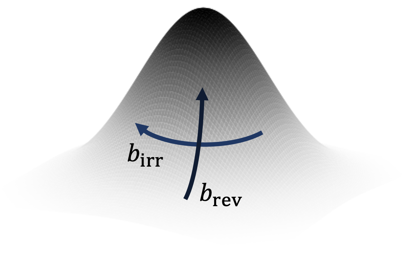
Armed with the time-reversal of diffusions we proceed to decompose the SDE into its time-reversible and time-irreversible components. This decomposition is called the Helmholtz decomposition because it can be obtained geometrically by decomposing the drift vector field b𝑏b into horizontal birrsubscript𝑏irrb_{\mathrm{irr}} (time-irreversible, conservative) and vertical brevsubscript𝑏revb_{\mathrm{rev}} (time-reversible, non-conservative) components with respect to the stationary density [11]. These vector fields are called horizontal and vertical, respectively, because the first flows along the contours of the stationary density, while the second ascends the landscape of the stationary density (see the schematic in the upper-left panel of Figure 1). For our purposes, we provide a self-contained, non-geometric proof of the Helmholtz decomposition in Appendix A.2.3.

Proposition 3.7 (Helmholtz decomposition).

Consider the solution (xt)t[0,T]subscriptsubscript𝑥𝑡𝑡0𝑇(x_{t})_{t\in[0,T]} of the Itô SDE (5) with coefficients satisfying Assumption 3.3. Let a probability density ρ𝜌\rho satisfying (Dρ)Lloc1(d,d)𝐷𝜌subscriptsuperscript𝐿1locsuperscript𝑑superscript𝑑\nabla\cdot(D\rho)\in L^{1}_{\mathrm{loc}}(\mathbb{R}^{d},\mathbb{R}^{d}). Then, the following are equivalent:

  1. 1.

    The density ρ𝜌\rho is stationary for (xt)t[0,T]subscriptsubscript𝑥𝑡𝑡0𝑇(x_{t})_{t\in[0,T]}.

  2. 2.

    We can write the drift as

    b=brev+birrbrev={Dlogρ+Dif ρ(x)>00if ρ(x)=0(birrρ)=0.𝑏subscript𝑏revsubscript𝑏irrsubscript𝑏revcases𝐷𝜌𝐷if 𝜌𝑥0otherwise0if 𝜌𝑥0otherwisesubscript𝑏irr𝜌0\begin{split}b&=b_{\mathrm{rev}}+b_{\mathrm{irr}}\\ b_{\mathrm{rev}}&=\begin{cases}D\nabla\log\rho+\nabla\cdot D\quad\text{if }\rho(x)>0\\ 0\quad\text{if }\rho(x)=0\end{cases}\\ \nabla\cdot(b_{\mathrm{irr}}\rho)&=0.\end{split} (9)

Furthermore, brevsubscript𝑏revb_{\mathrm{rev}} is time-reversible, while birrsubscript𝑏irrb_{\mathrm{irr}} is time-irreversible, i.e.,

b=brev+birr,b¯=brevbirr.formulae-sequence𝑏subscript𝑏revsubscript𝑏irr¯𝑏subscript𝑏revsubscript𝑏irr\displaystyle b=b_{\mathrm{rev}}+b_{\mathrm{irr}},\quad\bar{b}=b_{\mathrm{rev}}-b_{\mathrm{irr}}.

The fundamental importance of the Helmholtz decomposition was originally recognised in the context of non-equilibrium thermodynamics by Graham in 1977 [7], but its inception in this field dates from much earlier: for instance, the divergence free vector field birrρsubscript𝑏irr𝜌b_{\mathrm{irr}}\rho is precisely the stationary probability current or flux introduced by Nelson in 1967 [15]. More recently, the decomposition has recurrently been used in non-equilibrium statistical physics [8, 9, 46, 10, 47, 48, 49], and in statistical machine learning as the basis of Monte-Carlo sampling schemes [12, 11, 50, 10].
Refer to caption
Refer to caption
Refer to caption
Refer to caption
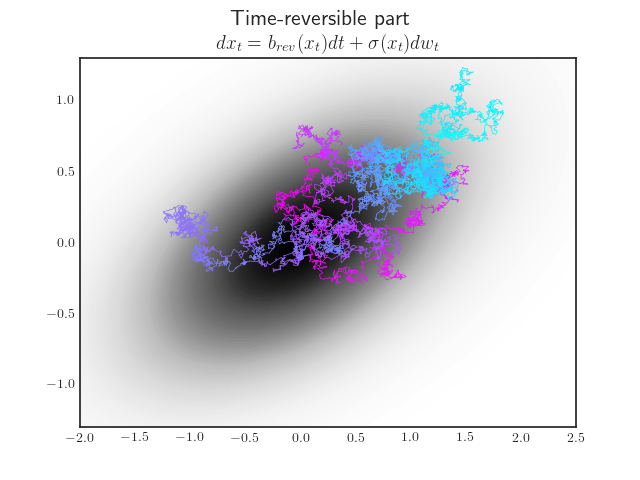
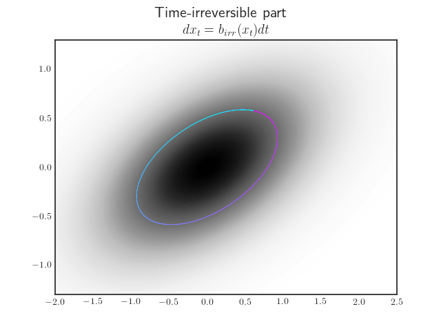
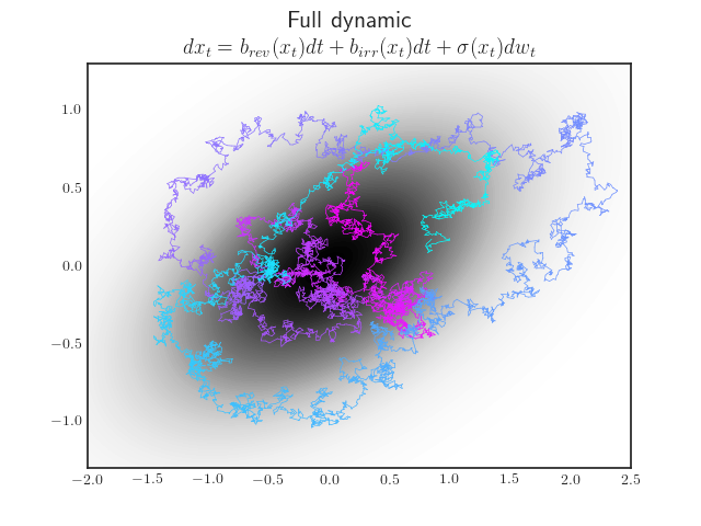
Figure 1: Helmholtz decomposition. The upper left panel illustrates the Helmholtz decomposition of the drift into time-reversible and time-irreversible parts: the time-reversible part of the drift flows towards the peak of the stationary density, while the time-irreversible part flows along its contours. The upper right panel shows a sample trajectory of a two-dimensional diffusion process stationary at a Gaussian distribution. The lower panels plot sample paths of the time-reversible (lower left) and time-irreversible (lower right) parts of the dynamic. Purely conservative dynamics (lower right) are reminiscent of the trajectories of massive bodies (e.g., planets) whose random fluctuations are negligible, as in Newtonian mechanics. Together, the lower panels illustrate time-irreversibility: If we were to reverse time, the trajectories of the time-reversible process would be statistically identical, while the trajectories of the time-irreversible process be distinguishable by flow, say, clockwise instead of counterclockwise. The full process (upper right) is a combination of both time-reversible and time-irreversible dynamics. The time-irreversible part defines a non-equilibrium steady-state and induces its characteristic wandering, cyclic behaviour.
Remark 3.8 (Probabilistic reversibility).

Here, time-reversible means reversibility in a probabilistic sense; that is, invariance under time reversal, also known as detailed balance [1, Proposition 3.3.4]. Probabilistic reversibility often leads to the non-conversation of quantities like the potential logρ(x)𝜌𝑥-\log\rho(x)For example, the identity (birrρ)=0subscript𝑏irr𝜌0\nabla\cdot(b_{\mathrm{irr}}\rho)=0 implies that the time-irreversible drift birrsubscript𝑏irrb_{\mathrm{irr}} flows along the contours of the probability density; in other words, the probability density and the potential are conserved along the time-irreversible vector field. In contrast, none of them are conserved when flowing along the time-reversible vector field brevsubscript𝑏revb_{\mathrm{rev}}. See Figure 1 for an illustration.

Remark 3.9 (Stratonovich formulation of Helmholtz decomposition).

There exists an equivalent decomposition of the drift of Stratonovich SDEs into time-reversible and irreversible parts. Assuming that σ𝜎\sigma is differentiable, we can rewrite the Itô SDE (5) into its equivalent Stratonovich SDE

dxt=bs(xt)dt+σ(xt)dwt.𝑑subscript𝑥𝑡superscript𝑏𝑠subscript𝑥𝑡𝑑𝑡𝜎subscript𝑥𝑡𝑑subscript𝑤𝑡\displaystyle dx_{t}=b^{s}(x_{t})dt+\sigma(x_{t})\circ dw_{t}.

where bs=bιsuperscript𝑏𝑠𝑏𝜄b^{s}=b-\iota and ι𝜄\iota is the Itô to Stratonovich correction [10, eq. 3.31]. Note that the correction is time-reversible. It follows that

birrssubscriptsuperscript𝑏𝑠irr\displaystyle b^{s}_{\mathrm{irr}} =birr,absentsubscript𝑏irr\displaystyle=b_{\mathrm{irr}}, (10)

and for x s.t. ρ(x)>0𝑥 s.t. 𝜌𝑥0x\text{ s.t. }\rho(x)>0,

brevs(x)subscriptsuperscript𝑏𝑠rev𝑥\displaystyle b^{s}_{\mathrm{rev}}(x) =(brevι)(x)=Dlogρ(x)+12σσ(x).absentsubscript𝑏rev𝜄𝑥𝐷𝜌𝑥12𝜎superscript𝜎top𝑥\displaystyle=(b_{\mathrm{rev}}-\iota)(x)=D\nabla\log\rho(x)+\frac{1}{2}\sigma\nabla\cdot\sigma^{\top}(x).

In particular, for x s.t. ρ(x)>0𝑥 s.t. 𝜌𝑥0x\text{ s.t. }\rho(x)>0,

bs(x)Rangeσ(x)superscript𝑏𝑠𝑥Range𝜎𝑥\displaystyle b^{s}(x)\in\operatorname{Range}\sigma(x) birrs(x)Rangeσ(x)iffabsentsubscriptsuperscript𝑏𝑠irr𝑥Range𝜎𝑥\displaystyle\iff b^{s}_{\mathrm{irr}}(x)\in\operatorname{Range}\sigma(x) (11)

as brevs(x)Rangeσ(x)subscriptsuperscript𝑏𝑠rev𝑥Range𝜎𝑥b^{s}_{\mathrm{rev}}(x)\in\operatorname{Range}\sigma(x). For diffusions driven by additive noise, Itô and Stratonovich formulations coincide bs=bsuperscript𝑏𝑠𝑏b^{s}=b. Thus, we conclude

σ is constant𝜎 is constant\displaystyle\sigma\text{ is constant} b(x)={Dlogρ(x)+birr(x)if ρ(x)>0birr(x)if ρ(x)=0absent𝑏𝑥cases𝐷𝜌𝑥subscript𝑏irr𝑥if 𝜌𝑥0otherwisesubscript𝑏irr𝑥if 𝜌𝑥0otherwise\displaystyle\Rightarrow b(x)=\begin{cases}D\nabla\log\rho(x)+b_{\mathrm{irr}}(x)\quad\text{if }\rho(x)>0\\ b_{\mathrm{irr}}(x)\quad\text{if }\rho(x)=0\end{cases}
(b(x)Rangeσ(x)birr(x)Rangeσ(x))\displaystyle\Rightarrow\left(b(x)\in\operatorname{Range}\sigma(x)\iff b_{\mathrm{irr}}(x)\in\operatorname{Range}\sigma(x)\right) (12)

These identities will be useful to compute the entropy production rate later on.

The time-irreversible part of the drift often takes a simple form:

Proposition 3.10 (Characterisation of time-irreversible drift).

Consider a smooth, strictly positive probability density ρ𝜌\rho and an arbitrary smooth vector field birrsubscript𝑏irrb_{\mathrm{irr}}. Then

(birrρ)=0birr=Qlogρ+Qiffsubscript𝑏irr𝜌0subscript𝑏irr𝑄𝜌𝑄\displaystyle\nabla\cdot(b_{\mathrm{irr}}\rho)=0\iff b_{\mathrm{irr}}=Q\nabla\log\rho+\nabla\cdot Q

where Q=Q𝑄superscript𝑄topQ=-Q^{\top} is a smooth antisymmetric matrix field.

A proof is provided in Appendix A.2.3. We conclude this section by unpacking the Helmholtz decomposition of underdamped Langevin dynamics.

Example 3.11 (Helmholtz decomposition of underdamped Langevin).

Following Example 3.6, it is straightforward to decompose underdamped Langevin dynamics into its time-irreversible and time-reversible parts. Indeed we just need to identify the parts of the drift whose sign changes, and remains invariant, under time reversal:

brev(q,p)=[0γM1p],birr(q,p)subscript𝑏rev𝑞𝑝matrix0𝛾superscript𝑀1𝑝subscript𝑏irr𝑞𝑝\displaystyle b_{\mathrm{rev}}(q,p)=\begin{bmatrix}0\\ -\gamma M^{-1}p\end{bmatrix},\quad b_{\mathrm{irr}}(q,p) =[M1pV(q)].absentmatrixsuperscript𝑀1𝑝𝑉𝑞\displaystyle=\begin{bmatrix}M^{-1}p\\ -\nabla V\left(q\right)\end{bmatrix}.

We can rewrite these in canonical form recalling the gradient of the stationary density (8)

brev(q,p)=Dlogρ(q,p),birr(q,p)=Qlogρ(q,p)formulae-sequencesubscript𝑏rev𝑞𝑝𝐷𝜌𝑞𝑝subscript𝑏irr𝑞𝑝𝑄𝜌𝑞𝑝\displaystyle b_{\mathrm{rev}}(q,p)=D\nabla\log\rho(q,p),\quad b_{\mathrm{irr}}(q,p)=Q\nabla\log\rho(q,p)
logρ(q,p)𝜌𝑞𝑝\displaystyle\nabla\log\rho(q,p) =β[V(q)M1p],D=[000γβ1Idn],Q=β1[0IdnIdn0].formulae-sequenceabsent𝛽matrix𝑉𝑞superscript𝑀1𝑝formulae-sequence𝐷matrix000𝛾superscript𝛽1subscriptId𝑛𝑄superscript𝛽1matrix0subscriptId𝑛subscriptId𝑛0\displaystyle=-\beta\begin{bmatrix}\nabla V(q)\\ M^{-1}p\end{bmatrix},\quad D=\begin{bmatrix}0&0\\ 0&\gamma\beta^{-1}\operatorname{Id}_{n}\end{bmatrix},\quad Q=\beta^{-1}\begin{bmatrix}0&-\operatorname{Id}_{n}\\ \operatorname{Id}_{n}&0\end{bmatrix}.

Clearly, the time-irreversible part of the process d[qt,pt]=birr(qt,pt)dtdsubscript𝑞𝑡subscript𝑝𝑡subscript𝑏irrsubscript𝑞𝑡subscript𝑝𝑡d𝑡\mathrm{d}[q_{t},p_{t}]=b_{\mathrm{irr}}(q_{t},p_{t})\mathrm{d}t is a Hamiltonian dynamic that preserves the energy (i.e., the Hamiltonian), while the time-reversible part is a reversible Ornstein-Uhlenbeck process. Example trajectories of the time-irreversible trajectory are exemplified in Figure 1 (bottom right).

3.5 Multiple perspectives on the Helmholtz decomposition

The Helmholtz decomposition is a cornerstone of the theory of diffusion processes. In addition to being a geometric decomposition of the drift [11], it is, equivalently, a time-reversible and irreversible decomposition of the SDE (13), of the generator and the (backward and forward) Kolmogorov PDEs describing the process. Briefly, the Helmholtz decomposition is equivalent to a functional analytic decomposition of the generator into symmetric and antisymmetric operators in a suitable function space. This corresponds to a decomposition of the backward Kolmogorov equation—which determines the evolution of (macroscopic) observables under the process—into a conservative and a dissipative flow. This decomposition can be used as a starting point to quantify the speed of convergence of the process to its stationary state from arbitrary initial conditions using hypocoercivity theory [24]. The same goes for the Fokker-Planck equation, which can be decomposed into a dissipative gradient flow, and a flow that is conservative in virtue of being orthogonal to the gradient flow in a suitable function space. This casts the Fokker-Planck equation in GENERIC form (General Equations for Non-Equilibrium Reversible-Irreversible Coupling), a general framework for analysing dynamical systems arising in non-equilibrium statistical physics [25, 23].

Below we outline these different equivalent perspectives. This section is provided for independent interest but will not be used to derive our main results on entropy production; you may conveniently skip it on a first reading.

3.5.1 Helmholtz decomposition of the SDE

Proposition 3.7 is equivalent to a Helmholtz decomposition of the SDE into its time-reversible and time-irreversible parts, noting that the volatility is invariant under time-reversal (Theorem 3.5)

dxt=birr(xt)dtTime-irreversible+brev(xt)dt+σ(xt)dwtTime-reversible.dsubscript𝑥𝑡subscriptsubscript𝑏irrsubscript𝑥𝑡d𝑡Time-irreversiblesubscriptsubscript𝑏revsubscript𝑥𝑡d𝑡𝜎subscript𝑥𝑡dsubscript𝑤𝑡Time-reversible\displaystyle\mathrm{d}x_{t}=\underbrace{b_{\mathrm{irr}}\left(x_{t}\right)\mathrm{d}t}_{\text{Time-irreversible}}+\underbrace{b_{\mathrm{rev}}\left(x_{t}\right)\mathrm{d}t+\sigma\left(x_{t}\right)\mathrm{d}w_{t}}_{\text{Time-reversible}}. (13)

Figure 1 illustrates this decomposition with simulations.

3.5.2 Helmholtz decomposition of the infinitesimal generator

Following the differential geometric viewpoint, a deterministic flow—namely, a vector field b𝑏b—is given by a first order differential operator b𝑏b\cdot\nabla. Similarly, a stochastic flow given by a diffusion—namely, a vector field b𝑏b and a diffusion tensor D𝐷D—is characterised by a second order differential operator

L=b+D,L𝑏𝐷\displaystyle\operatorname{L}=b\cdot\nabla+D\nabla\cdot\nabla, (14)

known as the generator. Note that the first order part is the deterministic flow given by the drift while the second order part is the stochastic flow determined by the diffusion. More precisely, the generator of a diffusion process solving the SDE (5) under Assumptions 3.3 and 3.4 is a linear, unbounded operator defined as

L:Cc(d)DomLLμp(d)Lμp(d),1p,Lf(y):=limt01t𝔼[f(xt)f(y)x0=y],\displaystyle\operatorname{L}:C_{c}^{\infty}(\mathbb{R}^{d})\subset\operatorname{Dom}\operatorname{L}\subset L^{p}_{\mu}(\mathbb{R}^{d})\to L^{p}_{\mu}(\mathbb{R}^{d}),1\leq p\leq\infty,\quad\operatorname{L}f(y):=\lim_{t\downarrow 0}\frac{1}{t}\mathbb{E}[f(x_{t})-f(y)\mid x_{0}=y], (15)
fDomL={fLμp(d)gLμp(d) s.t. 1t𝔼[f(xt)f(y)x0=y]t0g(y) in Lμp(d)}𝑓DomLconditional-set𝑓subscriptsuperscript𝐿𝑝𝜇superscript𝑑𝑔subscriptsuperscript𝐿𝑝𝜇superscript𝑑 s.t. 1𝑡𝔼delimited-[]𝑓subscript𝑥𝑡conditional𝑓𝑦subscript𝑥0𝑦𝑡0𝑔𝑦 in subscriptsuperscript𝐿𝑝𝜇superscript𝑑\displaystyle f\in\operatorname{Dom}\operatorname{L}=\left\{f\in L^{p}_{\mu}(\mathbb{R}^{d})\mid\exists g\in L^{p}_{\mu}(\mathbb{R}^{d})\text{ s.t. }\frac{1}{t}\mathbb{E}[f(x_{t})-f(y)\mid x_{0}=y]\xrightarrow{t\downarrow 0}g(y)\text{ in }L^{p}_{\mu}(\mathbb{R}^{d})\right\}

Diffusions are among the simplest and most canonical Markov processes because they are characterised by generators that are second order differential operators (with no constant part). Indeed, starting from (15), a quick computation using Itô’s formula yields (14).

Recall that we have a duality pairing ,μ:Lμp(d)Lμp(d):subscript𝜇tensor-productsubscriptsuperscript𝐿superscript𝑝𝜇superscript𝑑subscriptsuperscript𝐿𝑝𝜇superscript𝑑\langle\cdot,\cdot\rangle_{\mu}:L^{p^{\prime}}_{\mu}(\mathbb{R}^{d})\otimes L^{p}_{\mu}(\mathbb{R}^{d})\to\mathbb{R} defined by f,gμ=dfgdμsubscript𝑓𝑔𝜇subscriptsuperscript𝑑𝑓𝑔differential-d𝜇\langle f,g\rangle_{\mu}=\int_{\mathbb{R}^{d}}fg\>\mathrm{d}\mu, where 1p+1p=11superscript𝑝1𝑝1\frac{1}{p^{\prime}}+\frac{1}{p}=1.

A well-known fact is that the generator L¯¯L\bar{\operatorname{L}} of the time-reversed diffusion is the adjoint of the generator under the above duality pairing [51, 52], [1, Thm 4.3.2]. The adjoint L¯¯L\bar{\operatorname{L}} is implicitly defined by the relation

f,Lgμ=L¯f,gμ,fDomL¯,gDomL,formulae-sequencesubscript𝑓L𝑔𝜇subscript¯L𝑓𝑔𝜇formulae-sequencefor-all𝑓Dom¯L𝑔DomL\displaystyle\langle f,\operatorname{L}g\rangle_{\mu}=\langle\bar{\operatorname{L}}f,g\rangle_{\mu},\forall f\in\operatorname{Dom}\bar{\operatorname{L}},g\in\operatorname{Dom}\operatorname{L},
DomL¯=Dom¯Labsent\displaystyle\operatorname{Dom}\bar{\operatorname{L}}=\> {fLμ1(d)hLμ1(d),gDomL:f,Lgμ=h,gμ}.conditional-set𝑓subscriptsuperscript𝐿1𝜇superscript𝑑:formulae-sequencesubscriptsuperscript𝐿1𝜇superscript𝑑for-all𝑔DomLsubscript𝑓L𝑔𝜇subscript𝑔𝜇\displaystyle\{f\in L^{1}_{\mu}(\mathbb{R}^{d})\mid\exists h\in L^{1}_{\mu}(\mathbb{R}^{d}),\forall g\in\operatorname{Dom}\operatorname{L}:\langle f,\operatorname{L}g\rangle_{\mu}=\langle h,g\rangle_{\mu}\}.

(The concept of adjoint generalises the transpose of a matrix in linear algebra to operators on function spaces). The proof of Lemma 3.2 explicitly computes the adjoint and shows that it is a linear operator L¯:Lμ1(d)Lμ1(d):¯Lsubscriptsuperscript𝐿1𝜇superscript𝑑subscriptsuperscript𝐿1𝜇superscript𝑑\bar{\operatorname{L}}:L^{1}_{\mu}(\mathbb{R}^{d})\to L^{1}_{\mu}(\mathbb{R}^{d}) which equals

L¯f¯L𝑓\displaystyle\bar{\operatorname{L}}f =bf+2ρ1(Dρ)f+Df.absent𝑏𝑓2superscript𝜌1𝐷𝜌𝑓𝐷𝑓\displaystyle=-b\cdot\nabla f+2\rho^{-1}\nabla\cdot(D\rho)\cdot\nabla f+D\nabla\cdot\nabla f.

Notice how the first order part of the adjoint generator is the drift of the time-reversed diffusion, while the second order part is its diffusion, as expected (cf. Theorem 3.5).

Much like we derived the Helmholtz decomposition of the drift by identifying the time-reversible and irreversible parts (see the proof of Proposition 3.7), we proceed analogously at the level of the generator. Indeed, just as any matrix can be decomposed into a sum of antisymmetric and symmetric matrices, we may decompose the generator into a sum of antisymmetric and symmetric operators

L=A+S,A:=(LL¯)/2,S:=(L+L¯)/2,DomA=DomS=DomLDomL¯.\begin{split}\operatorname{L}&=\operatorname{A}+\operatorname{S},\quad\operatorname{A}:=\left(\operatorname{L}-\bar{\operatorname{L}}\right)/2,\quad\operatorname{S}:=\left(\operatorname{L}+\bar{\operatorname{L}}\right)/2,\quad\operatorname{Dom}\operatorname{A}=\operatorname{Dom}\operatorname{S}=\operatorname{Dom}\operatorname{L}\cap\operatorname{Dom}\bar{\operatorname{L}}.\end{split} (16)

By its analogous construction, this decomposition coincides with the Helmholtz decomposition; indeed, the symmetric operator recovers the time-reversible part of the dynamic while the antisymmetric operator recovers the time-irreversible part. In a nutshell, the Helmholtz decomposition of the generator is as follows

LL\displaystyle\operatorname{L} =A+S,A=birrTime-irreversibleS=brev+DTime-reversible,absentASsubscriptAsubscript𝑏irrTime-irreversiblesubscriptSsubscript𝑏rev𝐷Time-reversible\displaystyle=\operatorname{A}+\operatorname{S},\quad\underbrace{\operatorname{A}=b_{\mathrm{irr}}\cdot\nabla}_{\text{Time-irreversible}}\quad\underbrace{\operatorname{S}=b_{\mathrm{rev}}\cdot\nabla+D\nabla\cdot\nabla}_{\text{Time-reversible}},

where the summands are symmetric and antisymmetric operators because they behave accordingly under the duality pairing:

Af,gμ=f,AgμAntisymmetric,f,gDomA,Sf,gμ=f,SgμSymmetric,f,gDomS.formulae-sequencesubscriptsubscriptA𝑓𝑔𝜇subscript𝑓A𝑔𝜇Antisymmetricfor-all𝑓𝑔DomAsubscriptsubscriptS𝑓𝑔𝜇subscript𝑓S𝑔𝜇Symmetricfor-all𝑓𝑔DomS\displaystyle\underbrace{\langle\operatorname{A}f,g\rangle_{\mu}=-\langle f,\operatorname{A}g\rangle_{\mu}}_{\text{Antisymmetric}},\quad\forall f,g\in\operatorname{Dom}\operatorname{A},\quad\underbrace{\langle\operatorname{S}f,g\rangle_{\mu}=\langle f,\operatorname{S}g\rangle_{\mu}}_{\text{Symmetric}},\quad\forall f,g\in\operatorname{Dom}\operatorname{S}.

Noting that SS-\operatorname{S} is a positive semi-definite operator, we can go slightly further and decompose it into its square roots. To summarise:

Proposition 3.12.

We can rewrite the generator of the diffusion process as L=AΣΣLAsuperscriptΣΣ\operatorname{L}=\operatorname{A}-\operatorname{\Sigma}^{*}\operatorname{\Sigma} where AA\operatorname{A} is the antisymmetric part of the generator, and ΣΣsuperscriptΣΣ-\operatorname{\Sigma}^{*}\operatorname{\Sigma} is the symmetric part, as defined in (16). Here superscript\cdot^{*} denotes the adjoint with respect to the duality pairing ,μsubscript𝜇\langle\cdot,\cdot\rangle_{\mu}. The operators have the following functional forms: Af=birrfA𝑓subscript𝑏irr𝑓\operatorname{A}f=b_{\mathrm{irr}}\cdot\nabla f, 2Σf=σf2Σ𝑓superscript𝜎top𝑓\sqrt{2}\operatorname{\Sigma}f=\sigma^{\top}\nabla f, 2Σg=logρσg(σg)2superscriptΣ𝑔𝜌𝜎𝑔𝜎𝑔\sqrt{2}\operatorname{\Sigma}^{*}g=-\nabla\log\rho\cdot\sigma g-\nabla\cdot(\sigma g).

A proof is provided in Appendix A.2.4.

3.5.3 Helmholtz decomposition of the backward Kolmogorov equation

We say that a real-valued function over the state-space of the process f:d:𝑓superscript𝑑f:\mathbb{R}^{d}\to\mathbb{R} is an observable. Intuitively, this is a macroscopic quantity that can be measured or observed in a physical process (e.g., energy or pressure) when the (microscopic) process is not easily accessible. The evolution of an observable f𝑓f given that the process is prepared at a deterministic initial condition is given by ft(x)=𝔼[f(xt)|x0=x]subscript𝑓𝑡𝑥𝔼delimited-[]conditional𝑓subscript𝑥𝑡subscript𝑥0𝑥f_{t}(x)=\mathbb{E}[f(x_{t})|x_{0}=x].

The backward Kolmogorov equation is a fundamental equation describing a Markov process, as it encodes the motion of observables

tft=Lft,f0=fDomL.formulae-sequencesubscript𝑡subscript𝑓𝑡Lsubscript𝑓𝑡subscript𝑓0𝑓DomL\partial_{t}f_{t}=\operatorname{L}f_{t},\quad f_{0}=f\in\operatorname{Dom}\operatorname{L}.

In other words, ft=𝔼[f(xt)|x0=x]subscript𝑓𝑡𝔼delimited-[]conditional𝑓subscript𝑥𝑡subscript𝑥0𝑥f_{t}=\mathbb{E}[f(x_{t})|x_{0}=x] solves the equation. This highlights the central importance of the generator as providing a concise summary of the process.

The Helmholtz decomposition entails a decomposition of the backward Kolmogorov equation

tut=Aft+Sft=(AΣΣ)ft,f0=fDomL.formulae-sequencesubscript𝑡subscript𝑢𝑡Asubscript𝑓𝑡Ssubscript𝑓𝑡AsuperscriptΣΣsubscript𝑓𝑡subscript𝑓0𝑓DomL\partial_{t}u_{t}=\operatorname{A}f_{t}+\operatorname{S}f_{t}=(\operatorname{A}-\operatorname{\Sigma}^{*}\operatorname{\Sigma})f_{t},\quad f_{0}=f\in\operatorname{Dom}\operatorname{L}. (17)

This decomposition is appealing, as it allows us to further characterise the contributions of the time-reversible and irreversible parts of the dynamic. Along the time-irreversible part of the backward Kolmogorov equation tft=Aftsubscript𝑡subscript𝑓𝑡Asubscript𝑓𝑡\partial_{t}f_{t}=\operatorname{A}f_{t}, the Lμ2(d)subscriptsuperscript𝐿2𝜇superscript𝑑L^{2}_{\mu}(\mathbb{R}^{d})-norm μ\|\cdot\|_{\mu} is conserved. Indeed, since AA\operatorname{A} is antisymmetric, Af,fμ=0subscriptA𝑓𝑓𝜇0\langle\operatorname{A}f,f\rangle_{\mu}=0 for every fDomA𝑓DomAf\in\operatorname{Dom}\operatorname{A}, and hence

tftμ2=2Aft,ftμ=0.subscript𝑡superscriptsubscriptnormsubscript𝑓𝑡𝜇22subscriptAsubscript𝑓𝑡subscript𝑓𝑡𝜇0\partial_{t}\left\|f_{t}\right\|_{\mu}^{2}=2\left\langle\operatorname{A}f_{t},f_{t}\right\rangle_{\mu}=0.

On the other hand, along the time-reversible part of the backward Kolmogorov equation generated by ΣΣsuperscriptΣΣ-\operatorname{\Sigma}^{*}\operatorname{\Sigma}, the Lμ2(d)subscriptsuperscript𝐿2𝜇superscript𝑑L^{2}_{\mu}(\mathbb{R}^{d})-norm is dissipated:

tftμ2=2ΣΣft,ftμ=2Σftμ20.subscript𝑡superscriptsubscriptnormsubscript𝑓𝑡𝜇22subscriptsuperscriptΣΣsubscript𝑓𝑡subscript𝑓𝑡𝜇2superscriptsubscriptnormΣsubscript𝑓𝑡𝜇20\partial_{t}\left\|f_{t}\right\|_{\mu}^{2}=-2\left\langle\operatorname{\Sigma}^{*}\operatorname{\Sigma}f_{t},f_{t}\right\rangle_{\mu}=-2\left\|\operatorname{\Sigma}f_{t}\right\|_{\mu}^{2}\leq 0.

This offers another perspective on the fact that the time-irreversible part of the dynamic is conservative, while the time-reversible part is dissipative—of the Lμ2(d)superscriptsubscript𝐿𝜇2superscript𝑑L_{\mu}^{2}(\mathbb{R}^{d})-norm.

Beyond this, hypocoercivity theory allows us to analyse the backward Kolmogorov equation, once one has written its Helmholtz decomposition. Hypocoercivity is a functional analytic theory developed to analyse abstract evolution equations of the form (17), originally devised to systematically study the speed of convergence to stationary state of kinetic diffusion processes like the underdamped Langevin dynamics and the Boltzmann equation. As an important result, the theory provides sufficient conditions on the operators A,ΣAΣ\operatorname{A},\operatorname{\Sigma} to ensure an exponentially fast convergence of the backward Kolmogorov equation to a fixed point [24, Theorems 18 & 24]. Dually, these convergence rates quantify the speed of convergence of the process to its stationary density from a given initial condition.

3.5.4 GENERIC decomposition of the Fokker-Planck equation

This perspective can also be examined directly from the Fokker-Planck equation. The Fokker-Planck equation is another fundamental equation describing a diffusion process: it encodes the evolution of the density of the process over time (when it exists). The Fokker-Planck equation is the L2(d)superscript𝐿2superscript𝑑L^{2}(\mathbb{R}^{d})-dual to the backward Kolmogorov equation. It reads

tρt=Lρt=(bρt+(Dρt)),subscript𝑡subscript𝜌𝑡superscriptLsubscript𝜌𝑡𝑏subscript𝜌𝑡𝐷subscript𝜌𝑡\displaystyle\partial_{t}\rho_{t}=\operatorname{L}^{\prime}\rho_{t}=\nabla\cdot(-b\rho_{t}+\nabla\cdot(D\rho_{t})),

where LsuperscriptL\operatorname{L}^{\prime} is the adjoint of the generator with respect to the standard duality pairing ,\langle\cdot,\cdot\rangle; in other words Lf,g=f,LgsuperscriptL𝑓𝑔𝑓L𝑔\langle\operatorname{L}^{\prime}f,g\rangle=\langle f,\operatorname{L}g\rangle where f,g=dfg(x)dx𝑓𝑔subscriptsuperscript𝑑𝑓𝑔𝑥differential-d𝑥\langle f,g\rangle=\int_{\mathbb{R}^{d}}fg(x)\>\mathrm{d}x.

The Helmholtz decomposition implies a decomposition of the Fokker-Planck equation into two terms: assuming for now that ρt,ρ>0subscript𝜌𝑡𝜌0\rho_{t},\rho>0 (e.g., if the diffusion is elliptic)

tρt=(birrρt)+(brevρt+(Dρt))=(birrρt)+(ρtρ1(Dρ)+(Dρt))=(birrρt)+(ρtDlogρtρ).subscript𝑡subscript𝜌𝑡subscript𝑏irrsubscript𝜌𝑡subscript𝑏revsubscript𝜌𝑡𝐷subscript𝜌𝑡subscript𝑏irrsubscript𝜌𝑡subscript𝜌𝑡superscript𝜌1𝐷𝜌𝐷subscript𝜌𝑡subscript𝑏irrsubscript𝜌𝑡subscript𝜌𝑡𝐷subscript𝜌𝑡𝜌\begin{split}\partial_{t}\rho_{t}&=\nabla\cdot(-b_{\mathrm{irr}}\rho_{t})+\nabla\cdot(-b_{\mathrm{rev}}\rho_{t}+\nabla\cdot(D\rho_{t}))\\ &=\nabla\cdot(-b_{\mathrm{irr}}\rho_{t})+\nabla\cdot(-\rho_{t}\rho^{-1}\nabla\cdot(D\rho)+\nabla\cdot(D\rho_{t}))\\ &=\nabla\cdot(-b_{\mathrm{irr}}\rho_{t})+\nabla\cdot\left(\rho_{t}D\nabla\log\frac{\rho_{t}}{\rho}\right).\end{split} (18)

We will see that this decomposition casts the Fokker-Planck equation in pre-GENERIC form.

GENERIC (General Equations for Non-Equilibrium Reversible-Irreversible Coupling) is an important theory for analysing dynamical systems arising in non-equilibrium statistical physics like the Fokker-Planck equation. The framework rose to prominence through the seminal work of Ottinger [25] and was later developed by the applied physics and engineering communities. Only recently, the framework developed into a rigorous mathematical theory. We refer to [23] for mathematical details. The following Proposition shows how we can rewrite the Fokker-Planck equation in pre-GENERIC form:

tρt=W(ρt)time-irreversibleMρt(dH[ρtρ])time-reversible,subscript𝑡subscript𝜌𝑡subscriptWsubscript𝜌𝑡time-irreversiblesubscriptsubscriptMsubscript𝜌𝑡dHconditionalsubscript𝜌𝑡𝜌time-reversible\displaystyle\partial_{t}\rho_{t}=\underbrace{\operatorname{W}(\rho_{t})}_{\text{time-irreversible}}-\underbrace{\operatorname{M}_{\rho_{t}}\left(\mathrm{d}\operatorname{H}[\rho_{t}\mid\rho]\right)}_{\text{time-reversible}}, (19)
Proposition 3.13 (GENERIC decomposition of the Fokker-Planck equation).

The Fokker-Planck equation (18) is in pre-GENERIC form (19), with

W(ρt)=(birrρt),Mρt(dH[ρtρ])=(ρtDlogρtρ),formulae-sequence𝑊subscript𝜌𝑡subscript𝑏irrsubscript𝜌𝑡subscript𝑀subscript𝜌𝑡dHconditionalsubscript𝜌𝑡𝜌subscript𝜌𝑡𝐷subscript𝜌𝑡𝜌\displaystyle W(\rho_{t})=\nabla\cdot(-b_{\mathrm{irr}}\rho_{t}),\quad-M_{\rho_{t}}\left(\mathrm{d}\operatorname{H}[\rho_{t}\mid\rho]\right)=\nabla\cdot\left(\rho_{t}D\nabla\log\frac{\rho_{t}}{\rho}\right),
Mρt(ξ)=Σ(ρtΣξ)=(ρtDξ),dH[ρtρ]=logρtρ+1,formulae-sequencesubscript𝑀subscript𝜌𝑡𝜉superscriptΣsubscript𝜌𝑡Σ𝜉subscript𝜌𝑡𝐷𝜉dHconditionalsubscript𝜌𝑡𝜌subscript𝜌𝑡𝜌1\displaystyle M_{\rho_{t}}(\xi)=\Sigma^{\prime}(\rho_{t}\Sigma\xi)=-\nabla\cdot(\rho_{t}D\nabla\xi),\quad\mathrm{d}\operatorname{H}[\rho_{t}\mid\rho]=\log\frac{\rho_{t}}{\rho}+1,

where H[]\operatorname{H}[\cdot\mid\cdot] is the relative entropy, superscript\cdot^{\prime} denotes the adjoint under the standard duality pairing ,\langle\cdot,\cdot\rangle, dd\mathrm{d} is the Fréchet derivative in L2(d)superscript𝐿2superscript𝑑L^{2}(\mathbb{R}^{d}), and W,Mρt𝑊subscript𝑀subscript𝜌𝑡W,M_{\rho_{t}} satisfy the following relations:

  • Orthogonality: W(ρt),dH[ρtρ]=0Wsubscript𝜌𝑡dHconditionalsubscript𝜌𝑡𝜌0\langle\operatorname{W}(\rho_{t}),\mathrm{d}\operatorname{H}[\rho_{t}\mid\rho]\rangle=0,

  • Semi-positive definiteness: Mρt(h),g=h,Mρt(g)subscriptMsubscript𝜌𝑡𝑔subscriptMsubscript𝜌𝑡𝑔\langle\operatorname{M}_{\rho_{t}}(h),g\rangle=\langle h,\operatorname{M}_{\rho_{t}}(g)\rangle, and Mρt(g),g0subscriptMsubscript𝜌𝑡𝑔𝑔0\langle\operatorname{M}_{\rho_{t}}(g),g\rangle\geq 0.

A proof is provided in Appendix A.2.4.

Writing the Fokker-Planck equation in pre-GENERIC form (19) explicits the contributions of the time-reversible and time-irreversible parts at the level of density dynamics. Indeed, the relative entropy functional H[ρtρ]Hconditionalsubscript𝜌𝑡𝜌\operatorname{H}[\rho_{t}\mid\rho] is conserved along the time-irreversible part of the Fokker-Planck equation tρt=W(ρt)subscript𝑡subscript𝜌𝑡Wsubscript𝜌𝑡\partial_{t}\rho_{t}=\operatorname{W}(\rho_{t})

dH[ρtρ]dt=tρt,dH[ρtρ]=W(ρt),dH[ρtρ]=0.𝑑Hconditionalsubscript𝜌𝑡𝜌𝑑𝑡subscript𝑡subscript𝜌𝑡dHconditionalsubscript𝜌𝑡𝜌Wsubscript𝜌𝑡dHconditionalsubscript𝜌𝑡𝜌0\displaystyle\frac{d\operatorname{H}[\rho_{t}\mid\rho]}{dt}=\left\langle\partial_{t}\rho_{t},\mathrm{d}\operatorname{H}[\rho_{t}\mid\rho]\right\rangle=\langle\operatorname{W}(\rho_{t}),\mathrm{d}\operatorname{H}[\rho_{t}\mid\rho]\rangle=0.

Contrariwise, the relative entropy is dissipated along the time-reversible part of the equation

dH[ρtρ]dt=tρt,dH[ρtρ]=Mρt(dH[ρtρ]),dH[ρtρ]0.𝑑Hconditionalsubscript𝜌𝑡𝜌𝑑𝑡subscript𝑡subscript𝜌𝑡dHconditionalsubscript𝜌𝑡𝜌subscriptMsubscript𝜌𝑡dHconditionalsubscript𝜌𝑡𝜌dHconditionalsubscript𝜌𝑡𝜌0\displaystyle\frac{d\operatorname{H}[\rho_{t}\mid\rho]}{dt}=\left\langle\partial_{t}\rho_{t},\mathrm{d}\operatorname{H}[\rho_{t}\mid\rho]\right\rangle=-\left\langle\operatorname{M}_{\rho_{t}}\left(\mathrm{d}\operatorname{H}[\rho_{t}\mid\rho]\right),\mathrm{d}\operatorname{H}[\rho_{t}\mid\rho]\right\rangle\leq 0.

Aggregating these results, we obtain the well-known fact that the relative entropy with respect to the stationary density is a Lyapunov function of the Fokker-Planck equation; a result sometimes known as de Bruijn’s identity or Boltzmann’s H-theorem [53, Proposition 1.1].

4 The epsubscript𝑒𝑝e_{p} of stationary diffusions

We are now ready to investigate the entropy production of stationary diffusions. First, we give sufficient conditions guaranteeing the mutual absolute continuity of the forward and time-reversed path space measures and compute the entropy production rate. Second, we demonstrate that when these conditions fail the entropy production is infinite.

4.1 Regular case
Refer to caption
Refer to caption
Refer to caption
Refer to caption
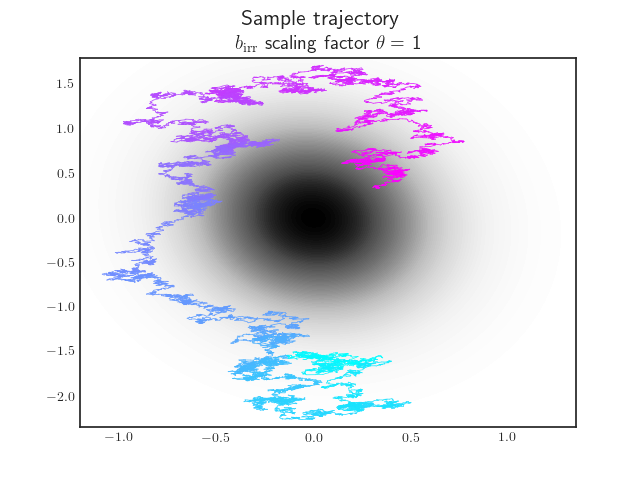
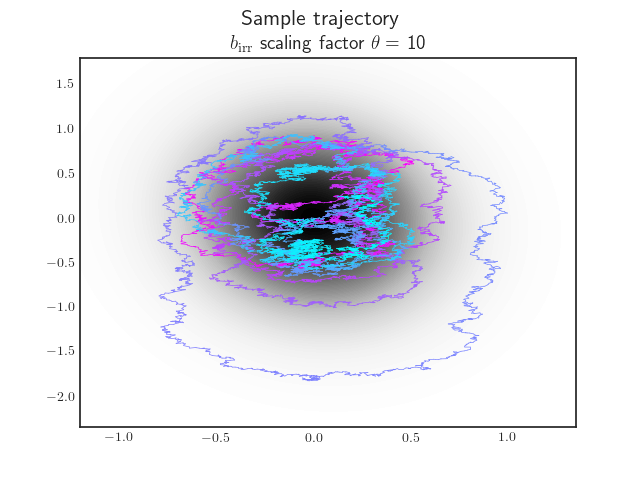
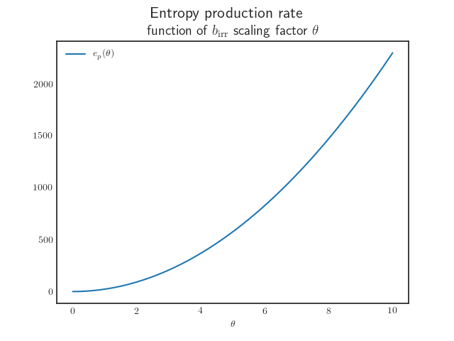
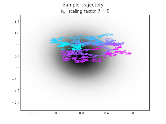
Figure 2: Entropy production as a function of time-irreversible drift. This figure illustrates the behaviour of sample paths and the entropy production rate as one scales the irreversible drift birrsubscript𝑏irrb_{\mathrm{irr}} by a parameter θ𝜃\theta. The underlying process is a two-dimensional Ornstein-Uhlenbeck process, for which exact sample paths and entropy production rate are available (Section 5.1). The heat map represents the density of the associated Gaussian steady-state. One sees that a non-zero irreversible drift induces circular, wandering behaviour around the contours of the steady-state, characteristic of a non-equilibrium steady-state (top right and bottom left). This is accentuated by increasing the strength of the irreversible drift. The entropy production rate measures the amount of irreversibility of the stationary process. It grows quadratically as a function of the irreversible scaling factor θ𝜃\theta (bottom right). When there is no irreversibility (top left), we witness an equilibrium steady-state. This is characterised by a vanishing entropy production (bottom right).
Theorem 4.1.

Let an Itô SDE (5) with coefficients satisfying Assumption 3.3. Assume that the solution (xt)t[0,T]subscriptsubscript𝑥𝑡𝑡0𝑇(x_{t})_{t\in[0,T]} is stationary with respect to a density ρ𝜌\rho satisfying Assumption 3.4. Denote by birrsubscript𝑏irrb_{\mathrm{irr}} the time-irreversible part of the drift (Proposition 3.7), and by superscript\cdot^{-} the Moore-Penrose matrix pseudo-inverse. Suppose that:

  1. 1.

    For ρ𝜌\rho-almost every xd𝑥superscript𝑑x\in\mathbb{R}^{d}, birr(x)Rangeσ(x)subscript𝑏irr𝑥Range𝜎𝑥b_{\mathrm{irr}}(x)\in\operatorname{Range}\sigma(x), and

  2. 2.

    The product σbirr:dm:superscript𝜎subscript𝑏irrsuperscript𝑑superscript𝑚\sigma^{-}b_{\mathrm{irr}}:\mathbb{R}^{d}\to\mathbb{R}^{m} is Borel measurable (e.g., if σbirrsuperscript𝜎subscript𝑏irr\sigma^{-}b_{\mathrm{irr}} is continuous), and

  3. 3.

    dbirrDbirrρ(x)dx<+subscriptsuperscript𝑑superscriptsubscript𝑏irrtopsuperscript𝐷subscript𝑏irr𝜌𝑥differential-d𝑥\int_{\mathbb{R}^{d}}b_{\mathrm{irr}}^{\top}D^{-}b_{\mathrm{irr}}\rho(x)\mathrm{d}x<+\infty.

Denote by 𝐏[0,T],𝐏¯[0,T]subscript𝐏0𝑇subscript¯𝐏0𝑇\mathbf{P}_{[0,T]},\bar{\mathbf{P}}_{[0,T]} the path space measures of the forward and time-reversed diffusions, respectively, on C([0,T],d)𝐶0𝑇superscript𝑑C([0,T],\mathbb{R}^{d}) (Definition 2.2). Then,

  1. 1.

    The path-space measures are equivalent 𝐏[0,T]𝐏¯[0,T]similar-tosubscript𝐏0𝑇subscript¯𝐏0𝑇\mathbf{P}_{[0,T]}\sim\bar{\mathbf{P}}_{[0,T]}, and

  2. 2.

    ep=dbirrDbirrρ(x)dxsubscript𝑒𝑝subscriptsuperscript𝑑superscriptsubscript𝑏irrtopsuperscript𝐷subscript𝑏irr𝜌𝑥differential-d𝑥e_{p}=\int_{\mathbb{R}^{d}}b_{\mathrm{irr}}^{\top}D^{-}b_{\mathrm{irr}}\rho(x)\mathrm{d}x.

Under the assumptions of Theorem 4.1, the epsubscript𝑒𝑝e_{p} is a quadratic form of the time-irreversible drift, see Figure 2.

A proof of Theorem 4.1 is provided in Appendix A.3.1. The idea of the proof is simple: in the elliptic case, the approach follows [1, Chapter 4] with some generalisations. In the non-elliptic case, the condition birr(x)Rangeσ(x)subscript𝑏irr𝑥Range𝜎𝑥b_{\mathrm{irr}}(x)\in\operatorname{Range}\sigma(x) intuitively ensures that the solution to the SDE, when initialised at any point, evolves on a sub-manifold of dsuperscript𝑑\mathbb{R}^{d} and is elliptic on this manifold (e.g., Figure 3). The pseudo-inverse of the diffusion tensor is essentially the inverse on this sub-manifold. Thus, a proof analogous to the elliptic case, but on the sub-manifold (essentially replacing all matrix inverses by pseudo-inverses and making sure everything still holds), shows that the path space measures of the forward and backward processes initialised at a given point are equivalent—and Girsanov’s theorem gives us their Radon-Nykodym derivative. Finally, Proposition 2.8 gives us the usual formula for the entropy production rate but with the matrix inverse replaced by the pseudo-inverse. Please see Section 6.3 for a geometric discussion of this proof.

Suppose either of assumptions 2, 3 of Theorem 4.1 do not hold. Then we have the following more general (and technical) result:

Theorem 4.2.

Let (Ω,,P)Ω𝑃(\Omega,\mathscr{F},P) be a probability space and (wt)t0subscriptsubscript𝑤𝑡𝑡0\left(w_{t}\right)_{t\geqslant 0} a standard Wiener process on msuperscript𝑚\mathbb{R}^{m}, with respect to the filtration (t)t0subscriptsubscript𝑡𝑡0(\mathscr{F}_{t})_{t\geq 0} [34, Definition 2.1.12]. Consider the Itô SDE (5) with coefficients satisfying Assumption 3.3. Consider its unique strong solution (xt)t[0,T]subscriptsubscript𝑥𝑡𝑡0𝑇(x_{t})_{t\in[0,T]} with respect to the given Brownian motion on the filtered probability space (Ω,,(t)t0,P)Ωsubscriptsubscript𝑡𝑡0𝑃(\Omega,\mathscr{F},(\mathscr{F}_{t})_{t\geq 0},P). Assume that the solution is stationary with respect to a density ρ𝜌\rho satisfying Assumption 3.4. Denote by birrsubscript𝑏irrb_{\mathrm{irr}} the time-irreversible part of the drift (Proposition 3.7), and by superscript\cdot^{-} the Moore-Penrose matrix pseudo-inverse. Suppose that:

  1. 1.

    For ρ𝜌\rho-almost every xd𝑥superscript𝑑x\in\mathbb{R}^{d}, birr(x)Rangeσ(x)subscript𝑏irr𝑥Range𝜎𝑥b_{\mathrm{irr}}(x)\in\operatorname{Range}\sigma(x), and

  2. 2.

    σbirr(xt)superscript𝜎subscript𝑏irrsubscript𝑥𝑡\sigma^{-}b_{\mathrm{irr}}(x_{t}) is an tsubscript𝑡\mathscr{F}_{t}-adapted process (e.g., σbirr:dm:superscript𝜎subscript𝑏irrsuperscript𝑑superscript𝑚\sigma^{-}b_{\mathrm{irr}}:\mathbb{R}^{d}\to\mathbb{R}^{m} is Borel measurable), and

  3. 3.

    The following holds

    𝔼P[ZT]=1,ZT:=exp(20Tσbirr(xt),dwt+|σbirr(xt)|2dt).formulae-sequencesubscript𝔼𝑃delimited-[]subscript𝑍𝑇1assignsubscript𝑍𝑇2superscriptsubscript0𝑇superscript𝜎subscript𝑏irrsubscript𝑥𝑡𝑑subscript𝑤𝑡superscriptsuperscript𝜎subscript𝑏irrsubscript𝑥𝑡2𝑑𝑡\mathbb{E}_{P}\left[Z_{T}\right]=1,Z_{T}:=\exp\left(-2\int_{0}^{T}\langle\sigma^{-}b_{\mathrm{irr}}(x_{t}),dw_{t}\rangle+|\sigma^{-}b_{\mathrm{irr}}(x_{t})|^{2}dt\right). (20)

Denote by 𝐏[0,T],𝐏¯[0,T]subscript𝐏0𝑇subscript¯𝐏0𝑇\mathbf{P}_{[0,T]},\bar{\mathbf{P}}_{[0,T]} the path space measures on C([0,T],d)𝐶0𝑇superscript𝑑C([0,T],\mathbb{R}^{d}) of the forward and time-reversed diffusions, respectively (Definition 2.2). Then,

  1. 1.

    The path-space measures are equivalent 𝐏[0,T]𝐏¯[0,T]similar-tosubscript𝐏0𝑇subscript¯𝐏0𝑇\mathbf{P}_{[0,T]}\sim\bar{\mathbf{P}}_{[0,T]}, and

  2. 2.

    ep=dbirrDbirrρ(x)dxsubscript𝑒𝑝subscriptsuperscript𝑑superscriptsubscript𝑏irrtopsuperscript𝐷subscript𝑏irr𝜌𝑥differential-d𝑥e_{p}=\int_{\mathbb{R}^{d}}b_{\mathrm{irr}}^{\top}D^{-}b_{\mathrm{irr}}\rho(x)\mathrm{d}x.

A proof is provided in Appendix A.3.1. The proof is similar to that of Theorem 4.1, but much shorter, since (20) allows one to apply Girsanov’s theorem directly; in contrast, a large part of the proof of Theorem 4.1 is dedicated to showing that indeed, a version of Girsanov’s theorem can be applied.

In relation to assumption 2 of Theorem 4.2, note that if a matrix field σ:dd×m:𝜎superscript𝑑superscript𝑑𝑚\sigma:\mathbb{R}^{d}\to\mathbb{R}^{d\times m} is Borel measurable, then its pseudo-inverse σ:dm×d:superscript𝜎superscript𝑑superscript𝑚𝑑\sigma^{-}:\mathbb{R}^{d}\to\mathbb{R}^{m\times d} is also Borel measurable. We now give sufficient conditions for the exponential condition (20).

Proposition 4.3.

Consider a stochastic process (xt)t[0,T]subscriptsubscript𝑥𝑡𝑡0𝑇(x_{t})_{t\in[0,T]} on the probability space (Ω,,(t)t0,P)Ωsubscriptsubscript𝑡𝑡0𝑃(\Omega,\mathscr{F},(\mathscr{F}_{t})_{t\geq 0},P), which is stationary at the density ρ𝜌\rho. Assume that σbirr(xt)superscript𝜎subscript𝑏irrsubscript𝑥𝑡\sigma^{-}b_{\mathrm{irr}}(x_{t}) is tsubscript𝑡\mathscr{F}_{t}-adapted. Then, either of the following conditions implies (20):

  1. 1.

    Zt=exp(20tσbirr(xs),dws+|σbirr(xs)|2ds),t[0,T]formulae-sequencesubscript𝑍𝑡2superscriptsubscript0𝑡superscript𝜎subscript𝑏irrsubscript𝑥𝑠𝑑subscript𝑤𝑠superscriptsuperscript𝜎subscript𝑏irrsubscript𝑥𝑠2𝑑𝑠𝑡0𝑇Z_{t}=\exp\left(-2{\int_{0}^{t}\langle\sigma^{-}b_{\mathrm{irr}}(x_{s}),dw_{s}\rangle+|\sigma^{-}b_{\mathrm{irr}}(x_{s})|^{2}ds}\right),t\in[0,T] is a martingale on the probability space (Ω,,{t}t0,P)Ωsubscriptsubscript𝑡𝑡0𝑃(\Omega,\mathscr{F},\{\mathscr{F}_{t}\}_{t\geq 0},P).

  2. 2.

    𝔼P(e20T|σbirr(xt)|2𝑑t)<+subscript𝔼𝑃superscript𝑒2superscriptsubscript0𝑇superscriptsuperscript𝜎subscript𝑏irrsubscript𝑥𝑡2differential-d𝑡\mathbb{E}_{P}\left(e^{2\int_{0}^{T}|\sigma^{-}b_{\mathrm{irr}}(x_{t})|^{2}dt}\right)<+\infty (Novikov’s condition).

  3. 3.

    There exists δ>0𝛿0\delta>0 such that 𝔼ρ(eδ|σbirr(x)|2)<+subscript𝔼𝜌superscript𝑒𝛿superscriptsuperscript𝜎subscript𝑏irr𝑥2\mathbb{E}_{\rho}\left(e^{\delta|\sigma^{-}b_{\mathrm{irr}}(x)|^{2}}\right)<+\infty.

  4. 4.

    supt[0,T]𝔼P[exp(0tσbirr(xs),dws)]<+subscriptsupremum𝑡0𝑇subscript𝔼𝑃delimited-[]superscriptsubscript0𝑡superscript𝜎subscript𝑏irrsubscript𝑥𝑠𝑑subscript𝑤𝑠\sup_{t\in[0,T]}\mathbb{E}_{P}\left[\exp\left(-\int_{0}^{t}\langle\sigma^{-}b_{\mathrm{irr}}(x_{s}),dw_{s}\rangle\right)\right]<+\infty (Kazamaki’s criterion).

  5. 5.

    There exists K<1𝐾1K<1 s.t. for all t[0,T]𝑡0𝑇t\in[0,T]

    𝔼P[2tT|σbirr(xt)|2𝑑s|t]K.subscript𝔼𝑃delimited-[]conditional2superscriptsubscript𝑡𝑇superscriptsuperscript𝜎subscript𝑏𝑖𝑟𝑟subscript𝑥𝑡2differential-d𝑠subscript𝑡𝐾\mathbb{E}_{P}\left[\left.2\int_{t}^{T}\left|\sigma^{-}b_{irr}(x_{t})\right|^{2}ds\>\right|\mathscr{F}_{t}\right]\leq K.
  6. 6.

    The tail of |σbirr(x)|2,xρsimilar-tosuperscriptsuperscript𝜎subscript𝑏irr𝑥2𝑥𝜌|\sigma^{-}b_{\mathrm{irr}}(x)|^{2},x\sim\rho decays exponentially fast, i.e., there exists positive constants c,C,R>0𝑐𝐶𝑅0c,C,R>0 such that for all r>R𝑟𝑅r>R

    P(|σbirr(x)|2>r)Cecr.𝑃superscriptsuperscript𝜎subscript𝑏irr𝑥2𝑟𝐶superscript𝑒𝑐𝑟\displaystyle P(|\sigma^{-}b_{\mathrm{irr}}(x)|^{2}>r)\leq Ce^{-cr}. (21)

Furthermore, (2 or 4) \Rightarrow 1; 5 \Rightarrow 2; and 6 \Rightarrow 3.

A proof is provided in Appendix A.3.1.

4.2 Singular case

When the time-irreversible part of the drift is not always in the range of the volatility matrix field, we have a different result.

Theorem 4.4.

Suppose that the Itô SDE (5) satisfies Assumption 3.3 and that the volatility is twice continuously differentiable σC2(d,d×m)𝜎superscript𝐶2superscript𝑑superscript𝑑𝑚\sigma\in C^{2}(\mathbb{R}^{d},\mathbb{R}^{d\times m}). Furthermore suppose that the solution (xt)t[0,T]subscriptsubscript𝑥𝑡𝑡0𝑇(x_{t})_{t\in[0,T]} is stationary with respect to a density ρ𝜌\rho satisfying Assumption 3.4. Denote by 𝐏[0,T],𝐏¯[0,T]subscript𝐏0𝑇subscript¯𝐏0𝑇\mathbf{P}_{[0,T]},\bar{\mathbf{P}}_{[0,T]} the path space measures on C([0,T],d)𝐶0𝑇superscript𝑑C([0,T],\mathbb{R}^{d}) of the forward and time-reversed processes, respectively (Definition 2.2). If birr(x)Rangeσ(x)subscript𝑏irr𝑥Range𝜎𝑥b_{\mathrm{irr}}(x)\in\operatorname{Range}\sigma(x) does not hold for ρ𝜌\rho-a.e. xd𝑥superscript𝑑x\in\mathbb{R}^{d}, then

𝐏[0,T]𝐏¯[0,T] and ep=+.perpendicular-tosubscript𝐏0𝑇subscript¯𝐏0𝑇 and subscript𝑒𝑝\displaystyle\mathbf{P}_{[0,T]}\perp\bar{\mathbf{P}}_{[0,T]}\text{ and }e_{p}=+\infty.

A proof is provided in Appendix A.3.2. The proof uses a version of the Stroock-Varadhan support theorem to show that there are paths that can be taken by the forward diffusion process that cannot be taken by the backward diffusion process—and vice-versa. Specifically, when considering the two processes initialised at a point xd𝑥superscript𝑑x\in\mathbb{R}^{d} where birr(x)Rangeσ(x)subscript𝑏irr𝑥Range𝜎𝑥b_{\mathrm{irr}}(x)\notin\operatorname{Range}\sigma(x), we can see that the derivatives of their respective possible paths at time 00 span different tangent sub-spaces at x𝑥x. Thus the path space measures 𝐏[0,T]x,𝐏¯[0,T]xsubscriptsuperscript𝐏𝑥0𝑇subscriptsuperscript¯𝐏𝑥0𝑇\mathbf{P}^{x}_{[0,T]},\bar{\mathbf{P}}^{x}_{[0,T]} are mutually singular. Since such x𝑥x occur with positive probability under the stationary density, it follows that the path space measures of the forward and time-reversed stationary processes 𝐏[0,T]x,𝐏¯[0,T]xsubscriptsuperscript𝐏𝑥0𝑇subscriptsuperscript¯𝐏𝑥0𝑇\mathbf{P}^{x}_{[0,T]},\bar{\mathbf{P}}^{x}_{[0,T]} are also mutually singular. Finally, the relative entropy between two mutually singular measures is infinity, hence the epsubscript𝑒𝑝e_{p} must be infinite.

By Theorem 4.4 and (12) we can readily see that the underdamped (7) and generalised Langevin [10, eq. 8.33] processes in phase-space have infinite entropy production. Expert statistical physicists will note that this contrasts with previous results in the literature stating that these diffusions have finite entropy production. There is no contradiction as physicists usually add an additional operator to the definition of the entropy production in these systems (Remark 2.7). While obviously informative of the underlying process, statistical physicists should take the results of Theorems 4.1, 4.2 and 4.4 to be physically relevant to entropy production insofar as the definition of entropy production we adopted (Definition 2.6) is physically meaningful for the system at hand. What if it is not? We will return to this in the discussion (Section 6.2).

In contrast to the underdamped and generalised Langevin equations, there exist hypoelliptic, non-elliptic diffusions with finite entropy production. For example, consider the following volatility matrix field

σ(x,y,z)=[x11101].𝜎𝑥𝑦𝑧matrix𝑥11101\displaystyle\sigma(x,y,z)=\begin{bmatrix}x&1\\ 1&1\\ 0&1\end{bmatrix}.

By Hörmander’s theorem [16, Theorem 1.3], for any smooth, confining (e.g., quadratic) potential V:3:𝑉superscript3V:\mathbb{R}^{3}\to\mathbb{R}, the process solving the SDE

dxt=DV(xt)dt+D(xt)dt+σ(xt)dwt𝑑subscript𝑥𝑡𝐷𝑉subscript𝑥𝑡𝑑𝑡𝐷subscript𝑥𝑡𝑑𝑡𝜎subscript𝑥𝑡𝑑subscript𝑤𝑡dx_{t}=-D\nabla V(x_{t})dt+\nabla\cdot D(x_{t})dt+\sigma(x_{t})dw_{t}

is hypoelliptic and non-elliptic. Furthermore, it is stationary and time-reversible at the Gibbs density ρ(x)exp(V(x))proportional-to𝜌𝑥𝑉𝑥\rho(x)\propto\exp(-V(x)).

5 Examples and epsubscript𝑒𝑝e_{p} of numerical simulations

We illustrate these results for linear diffusion processes, underdamped Langevin dynamics and their numerical simulations.

5.1 Linear diffusion processes

Given matrices Bd×d,σd×mformulae-sequence𝐵superscript𝑑𝑑𝜎superscript𝑑𝑚B\in\mathbb{R}^{d\times d},\sigma\in\mathbb{R}^{d\times m}, and a standard Brownian motion (wt)t[0,+)subscriptsubscript𝑤𝑡𝑡0(w_{t})_{t\in[0,+\infty)} on msuperscript𝑚\mathbb{R}^{m}, consider a linear diffusion process (i.e., a multivariate Ornstein-Uhlenbeck process)

dxt=b(xt)dt+σ(xt)dwt,b(x)=Bx,σ(x)σ.\begin{split}dx_{t}&=b(x_{t})dt+\sigma(x_{t})dw_{t},\quad b(x)=-Bx,\quad\sigma(x)\equiv\sigma.\end{split} (22)

This process arises, for example, in statistical physics as a model of the velocity of a massive Brownian particle subject to friction [54]; it covers the case of interacting particle systems when the interactions are linear in the states (e.g., the one dimensional ferromagnetic Gaussian spin model [55]); or when one linearises the equations of generic diffusion processes near the stationary density.

By solving the linear diffusion process (e.g., [55, Section 2.2]) one sees that the solution can be expressed as a linear operation on Brownian motion—a Gaussian process—thus the process must itself be Gaussian, and its stationary density as well (when it exists). Consider a Gaussian density ρ𝜌\rho

ρ(x)=𝒩(x;0,Π1),logρ(x)=12xΠx,formulae-sequence𝜌𝑥𝒩𝑥0superscriptΠ1𝜌𝑥12superscript𝑥topΠ𝑥\displaystyle\rho(x)=\mathcal{N}(x;0,\Pi^{-1}),\quad-\log\rho(x)=\frac{1}{2}x^{\top}\Pi x,

where Πd×dΠsuperscript𝑑𝑑\Pi\in\mathbb{R}^{d\times d} is the symmetric positive definite precision matrix. By the Helmholtz decomposition (Propositions 3.7 & 3.10), ρ𝜌\rho is a stationary density if and only if we can decompose the drift as follows:

b=brev+birr,brev(x)=DΠx,birr(x)=QΠx,formulae-sequence𝑏subscript𝑏revsubscript𝑏irrformulae-sequencesubscript𝑏rev𝑥𝐷Π𝑥subscript𝑏irr𝑥𝑄Π𝑥\displaystyle b=b_{\mathrm{rev}}+b_{\mathrm{irr}},\quad b_{\mathrm{rev}}(x)=-D\Pi x,\quad b_{\mathrm{irr}}(x)=-Q\Pi x,

where Q=Qd×d𝑄superscript𝑄topsuperscript𝑑𝑑Q=-Q^{\top}\in\mathbb{R}^{d\times d} is an arbitrary antisymmetric matrix, and, recall D=σσ/2d×d𝐷𝜎superscript𝜎top2superscript𝑑𝑑D=\sigma\sigma^{\top}/2\in\mathbb{R}^{d\times d} is the diffusion tensor. In particular, the drift of the forward and the time-reversed dynamic, are, respectively,

b(x)=Bx,B=(D+Q)Π,b¯(x)=Cx,C:=(DQ)Π.formulae-sequence𝑏𝑥𝐵𝑥formulae-sequence𝐵𝐷𝑄Πformulae-sequence¯𝑏𝑥𝐶𝑥assign𝐶𝐷𝑄Π\displaystyle b(x)=-Bx,\quad B=(D+Q)\Pi,\quad\bar{b}(x)=-Cx,\quad C:=(D-Q)\Pi.

Suppose that birr(x)Rangeσsubscript𝑏irr𝑥Range𝜎b_{\mathrm{irr}}(x)\in\operatorname{Range}\sigma for any xd𝑥superscript𝑑x\in\mathbb{R}^{d}. By definiteness of ΠΠ\Pi this is equivalent to RangeQRangeσRange𝑄Range𝜎\operatorname{Range}Q\subseteq\operatorname{Range}\sigma. By Theorem 4.1, and applying the trace trick to compute the Gaussian expectations of a bilinear form, we obtain444To obtain the last equality we used Tr(DDΠQ)=Tr(ΠQDD)=Tr(DDQΠ)Trsuperscript𝐷𝐷Π𝑄TrΠ𝑄superscript𝐷𝐷Tr𝐷superscript𝐷𝑄Π\operatorname{Tr}(D^{-}D\Pi Q)=\operatorname{Tr}(\Pi QD^{-}D)=-\operatorname{Tr}(DD^{-}Q\Pi). By standard properties of the pseudo-inverse DD𝐷superscript𝐷DD^{-} is the orthogonal projector onto RangeD=RangeσRange𝐷Range𝜎\operatorname{Range}D=\operatorname{Range}\sigma. Thus, RangeQRangeσRange𝑄Range𝜎\operatorname{Range}Q\subseteq\operatorname{Range}\sigma implies DDQ=Q𝐷superscript𝐷𝑄𝑄DD^{-}Q=Q. Finally, the trace of a symmetric matrix ΠΠ\Pi times an antisymmetric matrix Q𝑄Q vanishes.

ep=dbirrDbirrρ(x)dx=dxΠQDQΠxρ(x)dx=Tr(ΠQDQΠΠ1)=Tr(DQΠQ)=Tr(DBQ)+Tr(DDΠQ)=0=Tr(DBQ).subscript𝑒𝑝subscriptsuperscript𝑑superscriptsubscript𝑏irrtopsuperscript𝐷subscript𝑏irr𝜌𝑥differential-d𝑥subscriptsuperscript𝑑superscript𝑥topΠ𝑄superscript𝐷𝑄Π𝑥𝜌𝑥differential-d𝑥TrΠ𝑄superscript𝐷𝑄ΠsuperscriptΠ1Trsuperscript𝐷𝑄Π𝑄Trsuperscript𝐷𝐵𝑄subscriptTrsuperscript𝐷𝐷Π𝑄absent0Trsuperscript𝐷𝐵𝑄\begin{split}e_{p}&=\int_{\mathbb{R}^{d}}b_{\mathrm{irr}}^{\top}D^{-}b_{\mathrm{irr}}\rho(x)\mathrm{d}x=-\int_{\mathbb{R}^{d}}x^{\top}\Pi QD^{-}Q\Pi x\,\rho(x)\mathrm{d}x\\ &=-\operatorname{Tr}(\Pi QD^{-}Q\Pi\Pi^{-1})=-\operatorname{Tr}(D^{-}Q\Pi Q)\\ &=-\operatorname{Tr}(D^{-}BQ)+\underbrace{\operatorname{Tr}(D^{-}D\Pi Q)}_{=0}=-\operatorname{Tr}(D^{-}BQ).\end{split} (23)

This expression for the entropy production is nice as it generalises the usual formula to linear diffusion processes to degenerate noise, simply by replacing inverses with pseudo-inverses, cf. [55, eqs. 2.28-2.29] and [56, 57].

Contrariwise, suppose that RangeQRangeσnot-subset-of-or-equalsRange𝑄Range𝜎\operatorname{Range}Q\not\subseteq\operatorname{Range}\sigma. Then by Theorem 4.4,

ep=+.subscript𝑒𝑝\displaystyle e_{p}=+\infty. (24)

5.1.1 Exact numerical simulation and entropy production rate

Linear diffusion processes can be simulated exactly as their transition kernels are known. Indeed, by solving the process, one obtains the transition kernels of the Markov semigroup as a function of the drift and volatility [58, Theorem 9.1.1]. The forward and time-reserved transition kernels are the following:

pε(,x)=𝒩(eεBx,Sε),Sε:=0εetBσσetBdt,p¯ε(,x)=𝒩(eεCx,S¯ε),S¯ε:=0εetCσσetCdt.\begin{split}p_{\varepsilon}(\cdot,x)&=\mathcal{N}(e^{-\varepsilon B}x,S_{\varepsilon}),\quad S_{\varepsilon}:=\int_{0}^{\varepsilon}e^{-tB}\sigma\sigma^{\top}e^{-tB^{\top}}\mathrm{d}t,\\ \bar{p}_{\varepsilon}(\cdot,x)&=\mathcal{N}(e^{-\varepsilon C}x,\bar{S}_{\varepsilon}),\quad\bar{S}_{\varepsilon}:=\int_{0}^{\varepsilon}e^{-tC}\sigma\sigma^{\top}e^{-tC^{\top}}\mathrm{d}t.\end{split} (25)

Sampling from the transition kernels allows one to simulate the process exactly, and offers an alternative way to express the entropy production rate. Recall from Proposition 2.10 that the epsubscript𝑒𝑝e_{p} is the infinitesimal limit of the entropy production rate of an exact numerical simulation ep(ε)subscript𝑒𝑝𝜀e_{p}(\varepsilon) with time-step ε𝜀\varepsilon

epsubscript𝑒𝑝\displaystyle e_{p} =limε0ep(ε),ep(ε)=1ε𝔼xρ[H[pε(,x)p¯ε(,x)]].formulae-sequenceabsentsubscript𝜀0subscript𝑒𝑝𝜀subscript𝑒𝑝𝜀1𝜀subscript𝔼similar-to𝑥𝜌delimited-[]Hconditionalsubscript𝑝𝜀𝑥subscript¯𝑝𝜀𝑥\displaystyle=\lim_{\varepsilon\downarrow 0}e_{p}(\varepsilon),\quad e_{p}(\varepsilon)=\frac{1}{\varepsilon}\mathbb{E}_{x\sim\rho}[\operatorname{H}[p_{\varepsilon}(\cdot,x)\mid\bar{p}_{\varepsilon}(\cdot,x)]].

We can leverage the Gaussianity of the transition kernels to compute the relative entropy and obtain an alternative formula for the entropy production rate:

Lemma 5.1.

The entropy production rate of the stationary linear diffusion process can also be expressed as

ep=limε0ep(ε),ep(ε)=12ε[Tr(S¯εSε)rankσ+logdet(S¯ε)det(Sε)+Tr(Π1(eεCeεB)S¯ε(eεCeεB))],formulae-sequencesubscript𝑒𝑝subscript𝜀0subscript𝑒𝑝𝜀subscript𝑒𝑝𝜀12𝜀delimited-[]Trsuperscriptsubscript¯𝑆𝜀subscript𝑆𝜀rank𝜎superscriptdetsubscript¯𝑆𝜀superscriptdetsubscript𝑆𝜀TrsuperscriptΠ1superscriptsuperscript𝑒𝜀𝐶superscript𝑒𝜀𝐵topsuperscriptsubscript¯𝑆𝜀superscript𝑒𝜀𝐶superscript𝑒𝜀𝐵\begin{split}e_{p}&=\lim_{\varepsilon\downarrow 0}e_{p}(\varepsilon),\\ e_{p}(\varepsilon)&=\frac{1}{2\varepsilon}\left[\operatorname{Tr}(\bar{S}_{\varepsilon}^{-}S_{\varepsilon})-\operatorname{rank}\sigma+\log\frac{\operatorname{det}^{*}(\bar{S}_{\varepsilon})}{\operatorname{det}^{*}(S_{\varepsilon})}\right.\\ &\left.+\operatorname{Tr}\left(\Pi^{-1}(e^{-\varepsilon C}-e^{-\varepsilon B})^{\top}\bar{S}_{\varepsilon}^{-}(e^{-\varepsilon C}-e^{-\varepsilon B})\right)\right],\end{split} (26)

where superscript\cdot^{-} is the Moore-Penrose pseudo-inverse and detsuperscriptdet\operatorname{det}^{*} is the pseudo-determinant.

A proof is provided in Appendix A.4. Computing the limit (26) analytically, gives us back (23), (24), however, we will omit those details here. For our purposes, this gives us a way to numerically verify the value of epsubscript𝑒𝑝e_{p} that was obtained from theory. See Figures 3 and 4 for illustrations.
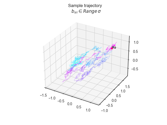
Refer to caption
Refer to caption
Refer to caption
Figure 3: Exact simulation of linear diffusion process with birr(x)Rangeσsubscript𝑏irr𝑥Range𝜎b_{\mathrm{irr}}(x)\in\operatorname{Range}\sigma. This figure considers an OU process in 3d space driven by degenerate noise, i.e., rankσ<3rank𝜎3\operatorname{rank}\sigma<3. The coefficients are such that σ=Q𝜎𝑄\sigma=Q are of rank 222. In particular, birr(x)Rangeσsubscript𝑏irr𝑥Range𝜎b_{\mathrm{irr}}(x)\in\operatorname{Range}\sigma holds for every x𝑥x. The process is not elliptic nor hypoelliptic, but it is elliptic over the subspace in which it evolves. The upper-left panel shows a sample trajectory starting from x0=(1,1,1)subscript𝑥0111x_{0}=(1,1,1). The upper-right panel shows samples from different trajectories after a time-step ε𝜀\varepsilon. There are only two principal components to this point cloud as the process evolves on a two dimensional subspace. In the bottom panel, we verify the theoretically predicted value of epsubscript𝑒𝑝e_{p} by evaluating the entropy production of an exact simulation ep(ε)subscript𝑒𝑝𝜀e_{p}(\varepsilon) with time-step ε𝜀\varepsilon. As predicted, we recover the true epsubscript𝑒𝑝e_{p} in the infinitesimal limit as the time-step of the exact simulation tends to zero ε0𝜀0\varepsilon\to 0. Furthermore, since the process is elliptic in its subspace, the entropy production is finite.
Refer to caption
Refer to caption
Refer to caption
Figure 4: Exact simulation of linear diffusion process with birr(x)Rangeσsubscript𝑏irr𝑥Range𝜎b_{\mathrm{irr}}(x)\not\in\operatorname{Range}\sigma. This figure considers an OU process in 3d space driven by degenerate noise. The coefficients are such that RangebirrRangesubscript𝑏irr\operatorname{Range}b_{\mathrm{irr}} is two-dimensional while RangeσRange𝜎\operatorname{Range}\sigma is one-dimensional, and such that the process does not satisfy Hörmander’s hypoellipticity condition. As such the process is hypoelliptic on a two-dimensional subspace; see a sample trajectory in the upper-left panel. By hypoellipticity its transition kernels are equivalent in the sense of measures, although far removed: On the upper right panel we show samples from different trajectories after a time-step ε𝜀\varepsilon. There are only two principal components to this data-cloud as the process evolves on a two dimensional subspace. In the bottom panel, we verify the theoretically predicted epsubscript𝑒𝑝e_{p} by evaluating the entropy production of an exact simulation ep(ε)subscript𝑒𝑝𝜀e_{p}(\varepsilon) with time-step ε𝜀\varepsilon. As predicted, we recover ep=+subscript𝑒𝑝e_{p}=+\infty in the infinitessimal limit as the time-step of the exact simulation tends to zero ε0𝜀0\varepsilon\downarrow 0. This turns out to be as the transition kernels of the forward and time-reversed processes become more and more mutually singular as the time-step decreases.

5.2 Underdamped Langevin dynamics

In this sub-section, we consider the entropy production rate of underdamped Langevin dynamics and its numerical simulations. Recall that the epsubscript𝑒𝑝e_{p} we compute here is defined without an additional momentum flip operator on the path space measure of the time-reversed process (i.e., (2) and not (3)), and may be a distinct quantity from the entropy production that physicists usually consider in such systems (see the discussion in Section 6.2).

Consider a Hamiltonian H(q,p)𝐻𝑞𝑝H(q,p) function of positions qn𝑞superscript𝑛q\in\mathbb{R}^{n} and momenta pn𝑝superscript𝑛p\in\mathbb{R}^{n} of the form

H(q,p)=V(q)+12pM1p𝐻𝑞𝑝𝑉𝑞12superscript𝑝topsuperscript𝑀1𝑝H(q,p)=V(q)+\frac{1}{2}p^{\top}M^{-1}p (27)

for some smooth potential function V:n:𝑉superscript𝑛V:\mathbb{R}^{n}\to\mathbb{R} and diagonal mass matrix Mn×n𝑀superscript𝑛𝑛M\in\mathbb{R}^{n\times n}.

The underdamped Langevin process is the solution to the SDE [27, eq 2.41]

{dqt=M1ptdtdpt=V(qt)dtγM1ptdt+2γβ1dwtcases𝑑subscript𝑞𝑡superscript𝑀1subscript𝑝𝑡𝑑𝑡otherwise𝑑subscript𝑝𝑡𝑉subscript𝑞𝑡𝑑𝑡𝛾superscript𝑀1subscript𝑝𝑡𝑑𝑡2𝛾superscript𝛽1𝑑subscript𝑤𝑡otherwise\begin{cases}dq_{t}=M^{-1}p_{t}dt\\ dp_{t}=-\nabla V\left(q_{t}\right)dt-\gamma M^{-1}p_{t}dt+\sqrt{2\gamma\beta^{-1}}dw_{t}\end{cases} (28)

for some friction coefficient γ>0𝛾0\gamma>0. This process arises in statistical physics, as a model of a particle coupled to a heat bath [59], [10, Chapter 8]; in Markov chain Monte-Carlo as an accelerated sampling scheme [45, 13]; and also as a model of interacting kinetic particles.

The invariant density, assuming it exists, is [27, Section 2.2.3.1]

ρ(q,p)=1ZeβH(q,p)=1ZeβV(q)eβ2pM1p.𝜌𝑞𝑝1𝑍superscript𝑒𝛽𝐻𝑞𝑝1𝑍superscript𝑒𝛽𝑉𝑞superscript𝑒𝛽2superscript𝑝topsuperscript𝑀1𝑝\displaystyle\rho(q,p)=\frac{1}{Z}e^{-\beta H(q,p)}=\frac{1}{Z}e^{-\beta V(q)}e^{-\frac{\beta}{2}p^{\top}M^{-1}p}.

Since the noise is additive the Itô interpretation of the SDE coincides with the Stratonovich interpretation, thus the irreversible drift is in the range of the volatility if and only if the drift is in the range of the volatility (12). Observe that when the momentum is non-zero p0𝑝0p\neq 0 the drift is not in the image of the volatility: in the q𝑞q components the drift is non-zero while the volatility vanishes. Since p0𝑝0p\neq 0 has full measure under the stationary density ρ(q,p)𝜌𝑞𝑝\rho(q,p) we obtain, from Theorem 4.4,

ep=+.subscript𝑒𝑝\displaystyle e_{p}=+\infty. (29)

Note that the entropy production of an exact numerical simulation with time-step ε>0𝜀0\varepsilon>0 is usually finite by hypoellipticity555(30) always holds in a quadratic potential, whence the process is a linear diffusion and the results from Section 5.1 apply. We conjecture this to hold in the non-linear case as well, as hypoellipticity guarantees that the transition kernels are mutually equivalent in the sense of measures.

ep(ε)<+.subscript𝑒𝑝𝜀\displaystyle e_{p}(\varepsilon)<+\infty. (30)

Figure 5 illustrates this with an exact simulation of underdamped Langevin dynamics in a quadratic potential.
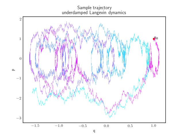
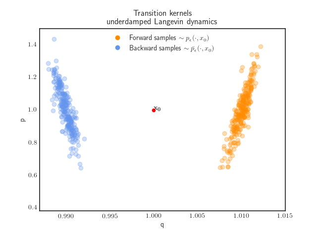
Refer to caption
Refer to caption
Refer to caption
Figure 5: Exact simulation of underdamped Langevin dynamics. This figure plots underdamped Langevin dynamics in a quadratic potential. Here, the process is two dimensional, i.e., positions and momenta evolve on the real line. We exploit the fact that underdamped Langevin in a quadratic potential is an Ornstein-Uhlenbeck process to simulate sample paths exactly. The choice of parameters was: V(q)=q2/2,M=γ=1formulae-sequence𝑉𝑞superscript𝑞22𝑀𝛾1V(q)=q^{2}/2,M=\gamma=1. The upper left panel plots a sample trajectory. One observes that the process is hypoelliptic: it is not confined to a prespecified region of space, cf. Figures 3, 4, even though random fluctuations affect the momenta only. The upper right panel plots samples of the forward and time-reversed processes after a time-step of ε𝜀\varepsilon. In the bottom panel, we verify the theoretically predicted epsubscript𝑒𝑝e_{p} by evaluating the entropy production of an exact simulation ep(ε)subscript𝑒𝑝𝜀e_{p}(\varepsilon) with time-step ε𝜀\varepsilon. As predicted, we recover ep=+subscript𝑒𝑝e_{p}=+\infty in the infinitessimal limit as the time-step of the exact simulation tends to zero ε0𝜀0\varepsilon\downarrow 0. This turns out to be because the transition kernels of the forward and time-reversed processes become more and more mutually singular as the time-step decreases.
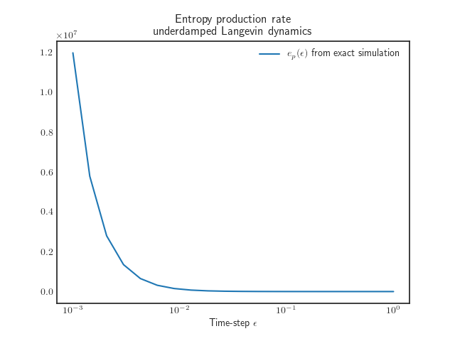
When the potential is non-quadratic, the underdamped process is a non-linear diffusion and one is usually unable to simulate it exactly. Instead, one resolves to numerical approximations to the solution of the process. We now turn to two common numerical discretisations of underdamped: the Euler-Maruyama and BBK discretisations. We will examine whether these discretisations are good approximations to the true process by computing their entropy production rate.

5.2.1 Euler-Maruyama discretisation

In this section, we show that an Euler-Maruyama (E-M) discretisation of underdamped Langevin dynamics at any time-step ε>0𝜀0\varepsilon>0 has infinite entropy production

epE-M(ε)=+.superscriptsubscript𝑒𝑝E-M𝜀\displaystyle e_{p}^{\text{E-M}}(\varepsilon)=+\infty. (31)

To see this, we take a step back and consider an arbitrary Itô SDE in dsuperscript𝑑\mathbb{R}^{d}

dxt=b(xt)dt+σ(xt)dwt𝑑subscript𝑥𝑡𝑏subscript𝑥𝑡𝑑𝑡𝜎subscript𝑥𝑡𝑑subscript𝑤𝑡\displaystyle dx_{t}=b(x_{t})dt+\sigma(x_{t})dw_{t}

The Euler-Maruyama discretisation for some time-step ε>0𝜀0\varepsilon>0 is

xi+1=xi+b(xi)ε+σ(xi)ωi,ωi𝒩(0,εIdd).formulae-sequencesubscript𝑥𝑖1subscript𝑥𝑖𝑏subscript𝑥𝑖𝜀𝜎subscript𝑥𝑖subscript𝜔𝑖similar-tosubscript𝜔𝑖𝒩0𝜀subscriptId𝑑\displaystyle x_{i+1}=x_{i}+b(x_{i})\varepsilon+\sigma(x_{i})\omega_{i},\quad\omega_{i}\sim\mathcal{N}(0,\varepsilon\operatorname{Id}_{d}).

This is a Markov chain with the following transition kernels

pεE-M(xi+1,xi)=𝒩(xi+1;xi+εb(xi),2εD(xi)),p¯εE-M(xi+1,xi):=pεE-M(xi,xi+1),formulae-sequencesubscriptsuperscript𝑝E-M𝜀subscript𝑥𝑖1subscript𝑥𝑖𝒩subscript𝑥𝑖1subscript𝑥𝑖𝜀𝑏subscript𝑥𝑖2𝜀𝐷subscript𝑥𝑖assignsubscriptsuperscript¯𝑝E-M𝜀subscript𝑥𝑖1subscript𝑥𝑖subscriptsuperscript𝑝E-M𝜀subscript𝑥𝑖subscript𝑥𝑖1\begin{split}p^{\text{E-M}}_{\varepsilon}\left(x_{i+1},x_{i}\right)&=\mathcal{N}(x_{i+1};x_{i}+\varepsilon b(x_{i}),2\varepsilon D(x_{i})),\\ \bar{p}^{\text{E-M}}_{\varepsilon}\left(x_{i+1},x_{i}\right)&:=p^{\text{E-M}}_{\varepsilon}\left(x_{i},x_{i+1}\right),\end{split} (32)

where p¯εE-Msubscriptsuperscript¯𝑝E-M𝜀\bar{p}^{\text{E-M}}_{\varepsilon} denotes the transition kernel of the backward chain666Caution: this is different from the E-M discretisation of the time-reversed process..

It turns out that when the SDE is not elliptic the transition kernels pεE-M(,x),p¯εE-M(,x)subscriptsuperscript𝑝E-M𝜀𝑥subscriptsuperscript¯𝑝E-M𝜀𝑥p^{\text{E-M}}_{\varepsilon}\left(\cdot,x\right),\bar{p}^{\text{E-M}}_{\varepsilon}\left(\cdot,x\right) tend to have different supports:

Lemma 5.2.

For any xd𝑥superscript𝑑x\in\mathbb{R}^{d}

supppεE-M(,x)suppsubscriptsuperscript𝑝E-M𝜀𝑥\displaystyle\operatorname{supp}p^{\mathrm{E}\text{-}\mathrm{M}}_{\varepsilon}\left(\cdot,x\right) ={y:yx+εb(x)+RangeD(x)}¯absent¯conditional-set𝑦𝑦𝑥𝜀𝑏𝑥Range𝐷𝑥\displaystyle=\overline{\{y:y\in x+\varepsilon b(x)+\operatorname{Range}D(x)\}}
suppp¯εE-M(,x)suppsubscriptsuperscript¯𝑝E-M𝜀𝑥\displaystyle\operatorname{supp}\bar{p}^{\mathrm{E}\text{-}\mathrm{M}}_{\varepsilon}\left(\cdot,x\right) ={y:xy+εb(y)+RangeD(y)}¯absent¯conditional-set𝑦𝑥𝑦𝜀𝑏𝑦Range𝐷𝑦\displaystyle=\overline{\{y:x\in y+\varepsilon b(y)+\operatorname{Range}D(y)\}}

Lemma 5.2 is immediate from (32) by noting that the support of p¯εE-M(,x)subscriptsuperscript¯𝑝E-M𝜀𝑥\bar{p}^{\text{E-M}}_{\varepsilon}\left(\cdot,x\right) is the closure of those elements whose successor by the forward process can be x𝑥x.

Unpacking the result of Lemma 5.2 in the case of underdamped Langevin dynamics yields

supppεE-M(,x)={y:yq=xq+εxp}¯,suppp¯εE-M(,x)={y:yq+εyp=xq}¯,formulae-sequencesuppsubscriptsuperscript𝑝E-M𝜀𝑥¯conditional-set𝑦subscript𝑦𝑞subscript𝑥𝑞𝜀subscript𝑥𝑝suppsubscriptsuperscript¯𝑝E-M𝜀𝑥¯conditional-set𝑦subscript𝑦𝑞𝜀subscript𝑦𝑝subscript𝑥𝑞\displaystyle\operatorname{supp}p^{\text{E-M}}_{\varepsilon}\left(\cdot,x\right)=\overline{\{y:y_{q}=x_{q}+\varepsilon x_{p}\}},\quad\operatorname{supp}\bar{p}^{\text{E-M}}_{\varepsilon}\left(\cdot,x\right)=\overline{\{y:y_{q}+\varepsilon y_{p}=x_{q}\}},

where x:=(xq,xp)assign𝑥subscript𝑥𝑞subscript𝑥𝑝x:=(x_{q},x_{p}) respectively denote position and momenta. One can see that pεE-M(,x)p¯εE-M(,x),xdformulae-sequenceperpendicular-tosubscriptsuperscript𝑝E-M𝜀𝑥subscriptsuperscript¯𝑝E-M𝜀𝑥for-all𝑥superscript𝑑p^{\text{E-M}}_{\varepsilon}\left(\cdot,x\right)\perp\bar{p}^{\text{E-M}}_{\varepsilon}\left(\cdot,x\right),\forall x\in\mathbb{R}^{d}. From Definition 2.11, we deduce that the entropy production rate of E-M applied to the underdamped process is infinite for any time-step ε>0𝜀0\varepsilon>0.

Refer to caption
Refer to caption
Figure 6: Euler-Maruyama simulation of underdamped Langevin dynamics. This figure compares the Euler-Maruyama simulation of underdamped Langevin dynamics with the exact simulation available in Figure 5. The choice of parameters was the same: V(q)=q2/2,M=γ=1formulae-sequence𝑉𝑞superscript𝑞22𝑀𝛾1V(q)=q^{2}/2,M=\gamma=1. The upper left panel plots a sample trajectory of the numerical scheme. One observes that the numerical scheme is not confined to a prespecified region of space like the true process. The upper right panel plots samples of the numerical scheme after a time-step of ε𝜀\varepsilon (in orange) given an initial condition at x0subscript𝑥0x_{0} (in red). This is superimposed onto a heat map of the true transition kernel (in black). We see that samples from the numerical scheme are in the right region of space, but are confined to a subspace which is not aligned with the heat map of the true transition kernel. The support of the transition kernel of the time-reversed scheme is shown in blue. One sees that the supports of forward and reverse transition kernels are mutually singular, thus the entropy production of the numerical discretisation is infinite for any time-step, which differs from the true process which has finite entropy production for any positive time-step.

5.2.2 BBK discretisation

Contrariwise to Euler, the BBK integrator [26, 27] is a splitting scheme that when applied to underdamped Langevin yields absolutely continuous transition kernels. The numerical scheme consists of three intermediate steps

pi+12=piV(qi)ε2γM1piε2+2γβ1ωisubscript𝑝𝑖12subscript𝑝𝑖𝑉subscript𝑞𝑖𝜀2𝛾superscript𝑀1subscript𝑝𝑖𝜀22𝛾superscript𝛽1subscript𝜔𝑖\displaystyle p_{i+\frac{1}{2}}=p_{i}-\nabla V\left(q_{i}\right)\frac{\varepsilon}{2}-\gamma M^{-1}p_{i}\frac{\varepsilon}{2}+\sqrt{2\gamma\beta^{-1}}\omega_{i}
qi+1=qi+M1pi+12εsubscript𝑞𝑖1subscript𝑞𝑖superscript𝑀1subscript𝑝𝑖12𝜀\displaystyle q_{i+1}=q_{i}+M^{-1}p_{i+\frac{1}{2}}\varepsilon
pi+1=pi+12V(qi+1)ε2γM1pi+12ε2+2γβ1ωi+12subscript𝑝𝑖1subscript𝑝𝑖12𝑉subscript𝑞𝑖1𝜀2𝛾superscript𝑀1subscript𝑝𝑖12𝜀22𝛾superscript𝛽1subscript𝜔𝑖12\displaystyle p_{i+1}=p_{i+\frac{1}{2}}-\nabla V\left(q_{i+1}\right)\frac{\varepsilon}{2}-\gamma M^{-1}p_{i+\frac{1}{2}}\frac{\varepsilon}{2}+\sqrt{2\gamma\beta^{-1}}\omega_{i+\frac{1}{2}}

with ωi,ωi+12N(0,ε2Id)similar-tosubscript𝜔𝑖subscript𝜔𝑖12𝑁0𝜀2Id\omega_{i},\omega_{i+\frac{1}{2}}\sim N\left(0,\frac{\varepsilon}{2}\operatorname{Id}\right). Its stability and convergence properties were studied in [26, 27] and its ergodic properties in [60, 61, 62].

It was shown in [22, Theorem 4.3] that the BBK discretisation of the underdamped Langevin process is quasi time-reversible, so that

epBBKO(ε).superscriptsubscript𝑒𝑝BBK𝑂𝜀\displaystyle e_{p}^{\mathrm{BBK}}\leq O(\varepsilon). (33)

One sees from Figure 7 that the BBK integrator better approximates the transition kernels than E-M, however it still is largely inaccurate from the point of view of the entropy production rate as the simulation becomes reversible when the time-step tends to zero.
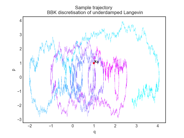
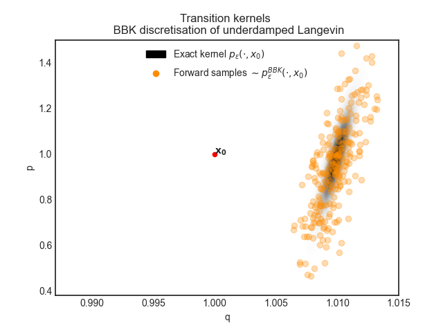
Refer to caption
Refer to caption
Refer to caption
Figure 7: BBK simulation of underdamped Langevin dynamics. This figure compares the BBK simulation of underdamped Langevin dynamics with the exact simulation available in Figure 5. The choice of parameters was the same: V(q)=q2/2,M=γ=1formulae-sequence𝑉𝑞superscript𝑞22𝑀𝛾1V(q)=q^{2}/2,M=\gamma=1. The upper left panel plots a sample trajectory of the numerical scheme. One observes that the numerical scheme is not confined to a prespecified region of space like the true process. The upper right panel plots samples of the numerical scheme after a time-step of ε𝜀\varepsilon (in orange) given an initial condition at x0subscript𝑥0x_{0} (in red). This is superimposed onto a heat map of the true transition kernel (in black). We see that samples from the numerical scheme fit the true transition kernel relatively well, but have a higher variance. The bottom panel estimates the entropy production rate of the numerical scheme for several choices of time-step ε𝜀\varepsilon. This is done by discretising the state-space into a number of bins and numerically evaluating the entropy production of the resulting Markov chain using samples, see Section 2.1 for details. The numerical values are consistent with the theoretical result (33).

5.2.3 Summary

In summary, the underdamped Langevin process has infinite entropy production rate in phase space777Recall that the epsubscript𝑒𝑝e_{p} we computed here is defined without an additional momentum flip operator on the path space measure of the time-reversed process, i.e., (2) and not (3). See also the discussion in Section 6.2,, but finite entropy production rate for any exact simulation with a positive time-step. When the potential is non-quadratic, the process is a non-linear diffusion that one usually cannot simulate exactly. To simulate it as accurately as possible, one should seek an approximating numerical scheme that has finite entropy production for any time-step, and whose entropy production tends to infinity for infinitesimally small time-steps.

Two well-known choices of numerical discretisation are the Euler-Maruyama and BBK schemes. By comparing their transition kernels with an exact simulation, we saw that the BBK scheme is a much better approximation to the true process than Euler-Maruyama. Analysis of the entropy production rate shows how these discretisations still far short in capturing important statistical properties of the process: the E-M discretisation has infinite entropy production for any time-step; while the BBK discretisation has finite entropy production for any time-step, and vanishing entropy production for infinitesimally small time-steps. Whenever possible, a good way to choose a time-step size for the BBK integrator might be matching its entropy production rate with that of an exact simulation. These results indicate that employing a BBK scheme with very small time-steps might be inadequate. Luckily, large step-sizes are usually preferred in practice.

In conclusion, the entropy production rate is a useful statistic of stochastic processes that can be used as a tool to devise accurate numerical schemes, particularly in a non-equilibrium statistical physics or sampling context where preserving the amount of time-irreversibility is important. Future development of numerical schemes should take entropy production into account; for example, in developing numerical schemes for underdamped Langevin, one should seek a finite entropy production rate for any positive time-step, which tends to infinity when time-steps become infinitesimally small. Other numerical schemes should be analysed in future work, such as those based on the lexicon for the approximation of the underdamped process developed by Leimkühler and Matthews [63, p. 269 & 271].

6 Discussion

Briefly, we unpack a couple of observations and possible extensions of this work.

6.1 epsubscript𝑒𝑝e_{p} and sampling efficiency

A well-known criterion for efficient sampling is time-irreversibility [21, 20, 64, 13]. Intuitively, non-reversible processes backtrack less often and thus furnish more diverse samples [65]. Furthermore, the time-irreversible part of the drift flows along the contours of the stationary probability density which yields mixing and accelerates convergence to the target measure. It is well known that removing non-reversibility worsens the spectral gap and the asymptotic variance of the MCMC estimator [20, 64, 21], which are two main indicators of the speed of convergence to stationary state [13]. Thus efficient samplers at non-equilibrium steady-state have positive entropy production.

In elliptic linear diffusions, one can construct the optimal time-irreversible drift to optimise the spectral gap [50, 66] or the asymptotic variance [64]. This indicates that one cannot optimise elliptic samplers by simply increasing their entropy production at steady-state without any other constraints, as, we recall, epsubscript𝑒𝑝e_{p} is a quadratic form of the strength of the time-irreversible drift (Figure 2).

Beyond this, the entropy production rate of general diffusions (Theorems 4.1, 4.2) bears a formal resemblance to the Donsker-Varadhan functional [20, Theorem 2.2], from which the asymptotic variance of MCMC estimators is derived [20]. It is entirely possible that one might be able to relate the non-stationary entropy production rate ((1) or [1, eq. 3.19]) to the Donsker-Varadhan functional, and thus give a more complete characterisation of sampling efficiency in terms of entropy production.

Many diffusion models of efficient sampling (the underdamped (7) and generalised [10, eq. 8.33] Langevin dynamics, the fastest converging linear diffusion [18]), and stochastic optimisation (stochastic gradient descent in deep neural networks [14]) are not elliptic; that is, they are driven by less Brownian drivers than there are dimensions to their phase space. In particular, these processes have their forward and backward path space measures which are mutually singular, and infinite entropy production888[14, Section 5] shows that stochastic gradient descent is out of equilibrium. Furthermore, it shows empirically that the rank of the diffusion matrix is about 1% of its dimension in deep neural networks. The sparsity of the noise with respect to the highly out-of-equilibrium behaviour they observe conjectures birr(x)Rangeσ(x)subscript𝑏irr𝑥Range𝜎𝑥b_{\mathrm{irr}}(x)\not\in\operatorname{Range}\sigma(x) and thus, mutual singularity of forward and backward path space measures.. In light of this, we conjecture that mutual singularity of the forward and backward path space measures is an important facet of sampling efficiency (provided the process is ergodic). Mutual singularity apparently exacerbates the mixing effect that time-irreversibility introduces in the elliptic case. Heuristically, if some paths can be taken by the forward process and not by the backward process, these trajectories cannot be reversed, thus the process is constantly forced to visit new regions of phase space, which contributes to the (non-reversible) convergence to steady-state.

If the above intuition holds, a useful statistic of sampling efficiency might be the probability that the forward process takes paths that cannot be taken by the backward process. By the Lebesgue decomposition theorem we can decompose the forward path space measure 𝐏𝐏\mathbf{P} into 𝐏reg+𝐏singsubscript𝐏regsubscript𝐏sing\mathbf{P}_{\textrm{reg}}+\mathbf{P}_{\textrm{sing}} such that 𝐏reg𝐏¯much-less-thansubscript𝐏reg¯𝐏\mathbf{P}_{\textrm{reg}}\ll\bar{\mathbf{P}} and 𝐏sing𝐏¯perpendicular-tosubscript𝐏sing¯𝐏\mathbf{P}_{\textrm{sing}}\perp\bar{\mathbf{P}}. This statistic is the non-negative real number

𝐏({γC([0,T],d):d𝐏/d𝐏¯(γ)=+})=𝐏sing(C([0,T],d)),𝐏conditional-set𝛾𝐶0𝑇superscript𝑑𝑑𝐏𝑑¯𝐏𝛾subscript𝐏sing𝐶0𝑇superscript𝑑\displaystyle\mathbf{P}(\{\gamma\in C([0,T],\mathbb{R}^{d}):d\mathbf{P}/d\bar{\mathbf{P}}(\gamma)=+\infty\})=\mathbf{P}_{\textrm{sing}}\left(C([0,T],\mathbb{R}^{d})\right),

where d𝐏/d𝐏¯𝑑𝐏𝑑¯𝐏d\mathbf{P}/d\bar{\mathbf{P}} is the Lebesgue derivative between forward and backward path space measures. Note that the linear diffusion that converges fastest to steady-state maximises the latter (under the constraint that the process remains ergodic) since it has only one Brownian driver [18]. However, this statistic does not tell us all since the direction of the Brownian driver with respect to the drift and the stationary density is important to determine sampling efficiency. Yet, these observations indicate that employing diffusions with less Brownian drivers might be an advantage for sampling and optimisation (provided ergodicity is maintained). A careful investigation of these relationships is left to future work.

6.2 Generalised non-reversibility and entropy production rate

Many diffusions studied in statistical physics are not time-reversible but they are generalised reversible; that is, they are time-reversible up to a one-to-one transformation θ𝜃\theta of phase-space which leaves the stationary measure invariant [23, Section 5.1], [27, eq. 2.32]. For example, the underdamped langevin equation is generalised reversible—it is reversible up to momentum reversal (Example 3.6); the generalised Langevin equation is also generalised reversible.

The entropy production, as defined in Definition 2.6, measures time-irreversibility as opposed to generalised non-reversibility. However, as pointed out in Remark 2.7, the physically meaningful definition of entropy production rate sometimes comprises additional operators applied to the path-space measure of the time-reversed process. This modified notion of epsubscript𝑒𝑝e_{p}, which we refer to as generalised entropy production, usually takes the form of

epgen,θ:=limε01εH[𝐏[0,ε],θ#𝐏¯[0,ε]],assignsuperscriptsubscript𝑒𝑝gen𝜃subscript𝜀01𝜀Hsubscript𝐏0𝜀subscript𝜃#subscript¯𝐏0𝜀e_{p}^{\mathrm{gen},\theta}:=\lim_{\varepsilon\downarrow 0}\frac{1}{\varepsilon}\operatorname{H}\left[\mathbf{P}_{[0,\varepsilon]},\theta_{\#}\bar{\mathbf{P}}_{[0,\varepsilon]}\right], (34)

where θ#subscript𝜃#\theta_{\#} is the pushforward operator associated to an involution of phase-space θ𝜃\theta that leaves the stationary distribution invariant. The generalised entropy production rate measures the generalised non-reversibility of the process; that is, the extent to which the process is time-irreversible up to the one-to-one transformation θ𝜃\theta. Of course, generalised entropy production reduces to entropy production, as defined in Definition 2.6, when θId𝜃Id\theta\equiv\operatorname{Id}.

Since generalised entropy production can sometimes be more physically meaningful, we spend the rest of this section computing it in a couple of examples.

It seems to be a general consensus in statistical physics that the physically relevant notion of entropy production for the underdamped Langevin process is the generalised entropy production when θ𝜃\theta is the momentum reversal [29, 30, 31, 67]. It is then a by-product of Example (3.6) that underdamped Langevin dynamics has zero (generalised) entropy production epgen,θ=0superscriptsubscript𝑒𝑝gen𝜃0e_{p}^{\mathrm{gen},\theta}=0, which contrasts with the infinite entropy production one obtains in the non-generalised case (Section 4.2) when one sets θId𝜃Id\theta\equiv\operatorname{Id}.

Beyond this, generalised entropy production could be a useful construct to quantify how far certain diffusion processes are from being generalised reversible. For example we can quantify to what extent certain time-irreversible perturbations of underdamped Langevin dynamics are far from being generalised reversible up to momentum reversal.

Example 6.1 (epgen,θsuperscriptsubscript𝑒𝑝gen𝜃e_{p}^{\mathrm{gen},\theta} of perturbed underdamped Langevin dynamics).

Consider the following perturbations of underdamped Langevin dynamics [68, eq. 8]

{dqt=M1ptdtQ1V(qt)dtdpt=V(qt)dtQ2M1ptdtγM1ptdt+2γβ1dwt,casesdsubscript𝑞𝑡superscript𝑀1subscript𝑝𝑡d𝑡subscript𝑄1𝑉subscript𝑞𝑡d𝑡otherwisedsubscript𝑝𝑡𝑉subscript𝑞𝑡d𝑡subscript𝑄2superscript𝑀1subscript𝑝𝑡d𝑡𝛾superscript𝑀1subscript𝑝𝑡d𝑡2𝛾superscript𝛽1dsubscript𝑤𝑡otherwise\begin{cases}\mathrm{d}q_{t}=M^{-1}p_{t}\mathrm{\leavevmode\nobreak\ d}t-Q_{1}\nabla V\left(q_{t}\right)\mathrm{d}t\\ \mathrm{d}p_{t}=-\nabla V\left(q_{t}\right)\mathrm{d}t-Q_{2}M^{-1}p_{t}\mathrm{\leavevmode\nobreak\ d}t-\gamma M^{-1}p_{t}\mathrm{\leavevmode\nobreak\ d}t+\sqrt{2\gamma\beta^{-1}}\mathrm{d}w_{t},\end{cases} (35)

where Q1,Q2d×dsubscript𝑄1subscript𝑄2superscript𝑑𝑑Q_{1},Q_{2}\in\mathbb{R}^{d\times d} are constant antisymmetric matrices. By inspection this equation has a Helmholtz decomposition that is similar to underdamped Langevin dynamics (cf. Example 3.11)

brev(q,p)=Dlogρ(q,p),birr(q,p)=Qlogρ(q,p)formulae-sequencesubscript𝑏rev𝑞𝑝𝐷𝜌𝑞𝑝subscript𝑏irr𝑞𝑝𝑄𝜌𝑞𝑝\displaystyle b_{\mathrm{rev}}(q,p)=D\nabla\log\rho(q,p),\quad b_{\mathrm{irr}}(q,p)=Q\nabla\log\rho(q,p)
logρ(q,p)𝜌𝑞𝑝\displaystyle\nabla\log\rho(q,p) =β[V(q)M1p],D=[000γβ1Idn],Q=β1[Q1IdnIdnQ2].formulae-sequenceabsent𝛽matrix𝑉𝑞superscript𝑀1𝑝formulae-sequence𝐷matrix000𝛾superscript𝛽1subscriptId𝑛𝑄superscript𝛽1matrixsubscript𝑄1subscriptId𝑛subscriptId𝑛subscript𝑄2\displaystyle=-\beta\begin{bmatrix}\nabla V(q)\\ M^{-1}p\end{bmatrix},\quad D=\begin{bmatrix}0&0\\ 0&\gamma\beta^{-1}\operatorname{Id}_{n}\end{bmatrix},\quad Q=\beta^{-1}\begin{bmatrix}Q_{1}&-\operatorname{Id}_{n}\\ \operatorname{Id}_{n}&Q_{2}\end{bmatrix}.

The time-reversed process solves the following SDE (Section 3.4)

{dq¯t=M1p¯tdt+Q1V(q¯t)dtdp¯t=V(q¯t)dt+Q2M1p¯tdtγM1p¯tdt+2γβ1dwt.casesdsubscript¯𝑞𝑡superscript𝑀1subscript¯𝑝𝑡d𝑡subscript𝑄1𝑉subscript¯𝑞𝑡d𝑡otherwisedsubscript¯𝑝𝑡𝑉subscript¯𝑞𝑡d𝑡subscript𝑄2superscript𝑀1subscript¯𝑝𝑡d𝑡𝛾superscript𝑀1subscript¯𝑝𝑡d𝑡2𝛾superscript𝛽1dsubscript𝑤𝑡otherwise\displaystyle\begin{cases}\mathrm{d}\bar{q}_{t}=-M^{-1}\bar{p}_{t}\mathrm{d}t+Q_{1}\nabla V\left(\bar{q}_{t}\right)\mathrm{d}t\\ \mathrm{d}\bar{p}_{t}=\nabla V\left(\bar{q}_{t}\right)\mathrm{d}t+Q_{2}M^{-1}\bar{p}_{t}\mathrm{\leavevmode\nobreak\ d}t-\gamma M^{-1}\bar{p}_{t}\mathrm{d}t+\sqrt{2\gamma\beta^{-1}}\mathrm{d}w_{t}.\end{cases}

Define θ(q,p)=(q,p)𝜃𝑞𝑝𝑞𝑝\theta(q,p)=(q,-p) to be the momentum reversal transformation of phase space (that leaves underdamped Langevin dynamics invariant as shown in Example 3.6). Letting p^t=p¯tsubscript^𝑝𝑡subscript¯𝑝𝑡\hat{p}_{t}=-\bar{p}_{t}, the time-reversed momentum-flipped equation looks like

{dq¯t=M1p^tdt+Q1V(q¯t)dtdp^t=V(q¯t)dt+Q2M1p^tdtγM1p^tdt+2γβ1dw^t.casesdsubscript¯𝑞𝑡superscript𝑀1subscript^𝑝𝑡d𝑡subscript𝑄1𝑉subscript¯𝑞𝑡d𝑡otherwisedsubscript^𝑝𝑡𝑉subscript¯𝑞𝑡d𝑡subscript𝑄2superscript𝑀1subscript^𝑝𝑡d𝑡𝛾superscript𝑀1subscript^𝑝𝑡d𝑡2𝛾superscript𝛽1dsubscript^𝑤𝑡otherwise\displaystyle\begin{cases}\mathrm{d}\bar{q}_{t}=M^{-1}\hat{p}_{t}\mathrm{d}t+Q_{1}\nabla V\left(\bar{q}_{t}\right)\mathrm{d}t\\ \mathrm{d}\hat{p}_{t}=-\nabla V\left(\bar{q}_{t}\right)\mathrm{d}t+Q_{2}M^{-1}\hat{p}_{t}\mathrm{\leavevmode\nobreak\ d}t-\gamma M^{-1}\hat{p}_{t}\mathrm{d}t+\sqrt{2\gamma\beta^{-1}}\mathrm{d}\hat{w}_{t}.\end{cases} (36)

Denote by birrgen,θsubscriptsuperscript𝑏gen𝜃irrb^{\mathrm{gen},\theta}_{\mathrm{irr}} the vector field whose sign changes after successively applying these two transformations:

birrgen,θ(q,p)=[Q1V(q)Q2M1p].subscriptsuperscript𝑏gen𝜃irr𝑞𝑝matrixsubscript𝑄1𝑉𝑞subscript𝑄2superscript𝑀1𝑝\displaystyle b^{\mathrm{gen},\theta}_{\mathrm{irr}}(q,p)=\begin{bmatrix}-Q_{1}\nabla V\left(q\right)\\ -Q_{2}M^{-1}p\end{bmatrix}.

It follows that the time-reversed, momentum-flipped equation (36) does not induce the same path space measure as the initial equation (35) unless Q1=Q2=0subscript𝑄1subscript𝑄20Q_{1}=Q_{2}=0. To see this, we follow the proofs of Theorems 4.4 and 4.1 to compute the generalised entropy production rate

Q10𝐏θ#𝐏¯epgen,θsubscript𝑄10𝐏perpendicular-tosubscript𝜃#¯𝐏superscriptsubscript𝑒𝑝gen𝜃\displaystyle Q_{1}\neq 0\Rightarrow\mathbf{P}\perp\theta_{\#}\bar{\mathbf{P}}\Rightarrow e_{p}^{\mathrm{gen},\theta} =+,absent\displaystyle=+\infty,
Q1=0𝐏θ#𝐏¯epgen,θsubscript𝑄10𝐏similar-tosubscript𝜃#¯𝐏superscriptsubscript𝑒𝑝gen𝜃\displaystyle Q_{1}=0\Rightarrow\mathbf{P}\sim\theta_{\#}\bar{\mathbf{P}}\Rightarrow e_{p}^{\mathrm{gen},\theta} =nbirrgen,θDbirrgen,θρ(q,p)dpdqabsentsubscriptdouble-integralsuperscript𝑛subscriptsuperscript𝑏gen𝜃irrsuperscript𝐷subscriptsuperscript𝑏gen𝜃irr𝜌𝑞𝑝differential-d𝑝differential-d𝑞\displaystyle=\iint_{\mathbb{R}^{n}}b^{\mathrm{gen},\theta}_{\mathrm{irr}}\cdot D^{-}b^{\mathrm{gen},\theta}_{\mathrm{irr}}\rho(q,p)\,\mathrm{d}p\,\mathrm{d}q
=γ1βn(Q2M1p)2ρ(p)dpabsentsuperscript𝛾1𝛽subscriptsuperscript𝑛superscriptsubscript𝑄2superscript𝑀1𝑝2𝜌𝑝differential-d𝑝\displaystyle=\gamma^{-1}\beta\int_{\mathbb{R}^{n}}(Q_{2}M^{-1}p)^{2}\rho(p)\mathrm{d}p
=γ1βTr(Q2M1Q2)<+.absentsuperscript𝛾1𝛽Trsubscript𝑄2superscript𝑀1subscript𝑄2\displaystyle=-\gamma^{-1}\beta\operatorname{Tr}\left(Q_{2}M^{-1}Q_{2}\right)<+\infty.

The last line equality follows from a standard result about expectations of bilinear forms under Gaussian distributions, since ρ(p)𝜌𝑝\rho(p) is Gaussian with covariance matrix M𝑀M. As usual, the generalised entropy production rate is a quadratic form of the (generalised) irreversible drift.

6.3 Geometric interpretation of results

Our main results concerning the value of entropy production have a straightforward geometric interpretation. The Stratonovich interpretation of the SDE

dxt=bs(xt)+σ(xt)dwt𝑑subscript𝑥𝑡superscript𝑏𝑠subscript𝑥𝑡𝜎subscript𝑥𝑡𝑑subscript𝑤𝑡\displaystyle dx_{t}=b^{s}(x_{t})+\sigma(x_{t})\circ dw_{t}

is the natural one to consider in a geometric context, when looking at the directions of the drift bssuperscript𝑏𝑠b^{s} and volatility vector fields σi,i=1,,mformulae-sequencesubscript𝜎absent𝑖𝑖1𝑚\sigma_{\cdot i},i=1,\ldots,m (i.e., the columns of the volatility matrix field).

Recall from Remark 3.9 that the Stratonovich SDE also admits a Helmholtz decomposition bs=brevs+birrssuperscript𝑏𝑠subscriptsuperscript𝑏𝑠revsubscriptsuperscript𝑏𝑠irrb^{s}=b^{s}_{\mathrm{rev}}+b^{s}_{\mathrm{irr}} with birrs=birrsubscriptsuperscript𝑏𝑠irrsubscript𝑏irrb^{s}_{\mathrm{irr}}=b_{\mathrm{irr}}, so that

bs(x)Rangeσ(x)birrs(x)Rangeσ(x)b¯s(x)Rangeσ(x) for any xsuppμ,iffsuperscript𝑏𝑠𝑥Range𝜎𝑥subscriptsuperscript𝑏𝑠irr𝑥Range𝜎𝑥iffsuperscript¯𝑏𝑠𝑥Range𝜎𝑥 for any 𝑥supp𝜇b^{s}(x)\in\operatorname{Range}\sigma(x)\iff b^{s}_{\mathrm{irr}}(x)\in\operatorname{Range}\sigma(x)\iff\bar{b}^{s}(x)\in\operatorname{Range}\sigma(x)\text{ for any }x\in\operatorname{supp}\mu, (37)

where b¯ssuperscript¯𝑏𝑠\bar{b}^{s} is the drift of the time-reversed Stratonovich SDE. In particular, time-reversal is a transformation that sends bssuperscript𝑏𝑠b^{s} to b¯ssuperscript¯𝑏𝑠\bar{b}^{s}, birrssuperscriptsubscript𝑏irr𝑠b_{\mathrm{irr}}^{s} to birrssuperscriptsubscript𝑏irr𝑠-b_{\mathrm{irr}}^{s}, or, equivalently, adds 2birrs2superscriptsubscript𝑏irr𝑠-2b_{\mathrm{irr}}^{s} to the drift.

Our main results can be summarised in a nutshell:

μ({xd:bs(x)Rangeσ(x)})=1ep=dbirrsDbirrsdμ(see Theorem 4.1 or 4.2 for details),μ({xd:bs(x)Rangeσ(x)})<1ep=+(see Theorem 4.4 for details).formulae-sequence𝜇conditional-set𝑥superscript𝑑superscript𝑏𝑠𝑥Range𝜎𝑥1subscript𝑒𝑝subscriptsuperscript𝑑superscriptsubscript𝑏irr𝑠superscript𝐷superscriptsubscript𝑏irr𝑠differential-d𝜇(see Theorem 4.1 or 4.2 for details)𝜇conditional-set𝑥superscript𝑑superscript𝑏𝑠𝑥Range𝜎𝑥1subscript𝑒𝑝(see Theorem 4.4 for details)\begin{split}\mu\left(\left\{x\in\mathbb{R}^{d}:b^{s}(x)\in\operatorname{Range}\sigma(x)\right\}\right)=1&\Rightarrow e_{p}=\int_{\mathbb{R}^{d}}b_{\mathrm{irr}}^{s}\cdot D^{-}b_{\mathrm{irr}}^{s}\mathrm{d}\mu\quad\text{(see Theorem \ref{thm: epr regular case simple} or \ref{thm: epr regular case general} for details)},\\ \mu\left(\left\{x\in\mathbb{R}^{d}:b^{s}(x)\in\operatorname{Range}\sigma(x)\right\}\right)<1&\Rightarrow e_{p}=+\infty\quad\text{(see Theorem \ref{thm: epr singular} for details)}.\end{split} (38)

We derived our main results using the Itô interpretation of an SDE because this allowed us to make more general statements, notably in the context of the general existence and uniqueness theorem of strong solutions to Itô SDEs; it turns out, however, that these results are more naturally interpreted in the Stratonovich context.

Consider the case where there is noise in the direction of the vector field bssuperscript𝑏𝑠b^{s}, (almost every-) where the process is; in other words, assume that μ({xd:bs(x)Rangeσ(x)})=1𝜇conditional-set𝑥superscript𝑑superscript𝑏𝑠𝑥Range𝜎𝑥1\mu\left(\left\{x\in\mathbb{R}^{d}:b^{s}(x)\in\operatorname{Range}\sigma(x)\right\}\right)=1. Consider the process at any point xsuppμ𝑥supp𝜇x\in\operatorname{supp}\mu. In virtue of (37), the drifts of the forward and time reversed processes both live in Rangeσ(x)Range𝜎𝑥\operatorname{Range}\sigma(x), the subset of the tangent space that is spanned by the volatility vector fields. Since the driving fluctuations are Gaussian on Rangeσ(x)Range𝜎𝑥\operatorname{Range}\sigma(x), the time-reversal transformation will be reversed by the random fluctuations with positive probability. Thus, the forward and time-reversed Markov transition kernels (for an infinitesimally small time-step) have the same support—they are mutually equivalent. Under sufficient regularity, made explicit in Theorems 4.1 or 4.2, their relative entropy is finite. The epsubscript𝑒𝑝e_{p} is the relative entropy between such Markov kernels on an infinitesimally small time-step (Proposition 2.10), so it too will be finite.

On the other hand, if there exists xsuppμ𝑥supp𝜇x\in\operatorname{supp}\mu such that there is no noise in the direction of the vector field bssuperscript𝑏𝑠b^{s}, that is bs(x)Rangeσ(x)superscript𝑏𝑠𝑥Range𝜎𝑥b^{s}(x)\not\in\operatorname{Range}\sigma(x), then the direction of the forward and time-reversed dynamics in an infinitesimal time-step lie on different tangent spaces, bs(x)+Rangeσ(x)superscript𝑏𝑠𝑥Range𝜎𝑥b^{s}(x)+\operatorname{Range}\sigma(x) and b¯s(x)+Rangeσ(x)superscript¯𝑏𝑠𝑥Range𝜎𝑥\bar{b}^{s}(x)+\operatorname{Range}\sigma(x), respectively. This means that the forward and time-reversed transition kernels (for an infinitesimally small time-step) are mutually singular and their relative entropy is infinite; thus, the epsubscript𝑒𝑝e_{p} is also infinite.

In particular, it should be straightforward to extend these observations and calculations to diffusions on manifolds.

Additional information

Data accessibility

All data and numerical simulations can be reproduced with code freely available at https://github.com/lancelotdacosta/entropy_production_stationary_diffusions.

Funding statement

LD is supported by the Fonds National de la Recherche, Luxembourg (Project code: 13568875). This publication is based on work partially supported by the EPSRC Centre for Doctoral Training in Mathematics of Random Systems: Analysis, Modelling and Simulation (EP/S023925/1). The work of GAP was partially funded by the EPSRC, grant number EP/P031587/1, and by JPMorgan Chase & Co. Any views or opinions expressed herein are solely those of the authors listed, and may differ from the views and opinions expressed by JPMorgan Chase & Co. or its affiliates. This material is not a product of the Research Department of J.P. Morgan Securities LLC. This material does not constitute a solicitation or offer in any jurisdiction.

Authors’ contributions

All authors made substantial contributions to conception and design, and writing of the article; and approved publication of the final version.

Competing interests

We have no competing interests.

Acknowledgements

We thank Dalton A. R. Sakthivadivel for interesting discussions. We are grateful to our anonymous reviewers for many helpful comments that improved the manuscript.

Appendix A Proofs

Here we provide proofs supporting the main text.

A.1 The epsubscript𝑒𝑝e_{p} of stationary Markov processes

A.1.1 epsubscript𝑒𝑝e_{p} in terms of path space measures with deterministic initial condition

We prove Proposition 2.8:

Proof.

The proof is straightforward

ep=1tH[𝐏[0,t]𝐏¯[0,t]]=1t𝔼x𝐏[logd𝐏[0,t]d𝐏¯[0,t](x)]=1t𝔼xμ[𝔼x𝐏[0,t]x[logd𝐏[0,t]d𝐏¯[0,t](x)]]=1t𝔼xμ[𝔼x𝐏[0,t]x[logd𝐏[0,t]xd𝐏¯[0,t]x(x)]]=1t𝔼xμ[H[𝐏[0,t]x𝐏¯[0,t]x]].subscript𝑒𝑝1𝑡Hconditionalsubscript𝐏0𝑡subscript¯𝐏0𝑡1𝑡subscript𝔼similar-tosubscript𝑥𝐏delimited-[]𝑑subscript𝐏0𝑡𝑑subscript¯𝐏0𝑡subscript𝑥1𝑡subscript𝔼similar-to𝑥𝜇delimited-[]subscript𝔼similar-tosubscript𝑥subscriptsuperscript𝐏𝑥0𝑡delimited-[]𝑑subscript𝐏0𝑡𝑑subscript¯𝐏0𝑡subscript𝑥1𝑡subscript𝔼similar-to𝑥𝜇delimited-[]subscript𝔼similar-tosubscript𝑥subscriptsuperscript𝐏𝑥0𝑡delimited-[]𝑑subscriptsuperscript𝐏𝑥0𝑡𝑑subscriptsuperscript¯𝐏𝑥0𝑡subscript𝑥1𝑡subscript𝔼similar-to𝑥𝜇delimited-[]Hconditionalsubscriptsuperscript𝐏𝑥0𝑡subscriptsuperscript¯𝐏𝑥0𝑡\begin{split}e_{p}&=\frac{1}{t}\operatorname{H}\left[\mathbf{P}_{[0,t]}\mid\bar{\mathbf{P}}_{[0,t]}\right]=\frac{1}{t}\mathbb{E}_{x_{\bullet}\sim\mathbf{P}}\left[\log\frac{d\mathbf{P}_{[0,t]}}{d\bar{\mathbf{P}}_{[0,t]}}(x_{\bullet})\right]\\ &=\frac{1}{t}\mathbb{E}_{x\sim\mu}\left[\mathbb{E}_{x_{\bullet}\sim\mathbf{P}^{x}_{[0,t]}}\left[\log\frac{d\mathbf{P}_{[0,t]}}{d\bar{\mathbf{P}}_{[0,t]}}(x_{\bullet})\right]\right]\\ &=\frac{1}{t}\mathbb{E}_{x\sim\mu}\left[\mathbb{E}_{x_{\bullet}\sim\mathbf{P}^{x}_{[0,t]}}\left[\log\frac{d\mathbf{P}^{x}_{[0,t]}}{d\bar{\mathbf{P}}^{x}_{[0,t]}}(x_{\bullet})\right]\right]=\frac{1}{t}\mathbb{E}_{x\sim\mu}\left[\operatorname{H}\left[\mathbf{P}^{x}_{[0,t]}\mid\bar{\mathbf{P}}^{x}_{[0,t]}\right]\right].\end{split}

A.1.2 epsubscript𝑒𝑝e_{p} in terms of transition kernels

We prove Proposition 2.10:

Proof.

By Proposition 2.8,

ep=limε01ε𝔼xμ[𝔼x𝐏[0,ε]x[logd𝐏[0,ε]xd𝐏¯[0,ε]x(x)]]=limε01ε𝔼xμ[𝔼ypε(,x)[logdpε(,x)dp¯ε(,x)(y)]]=limε01ε𝔼xμ[H[pε(,x)p¯ε(,x)]].subscript𝑒𝑝subscript𝜀01𝜀subscript𝔼similar-to𝑥𝜇delimited-[]subscript𝔼similar-tosubscript𝑥subscriptsuperscript𝐏𝑥0𝜀delimited-[]𝑑subscriptsuperscript𝐏𝑥0𝜀𝑑subscriptsuperscript¯𝐏𝑥0𝜀subscript𝑥subscript𝜀01𝜀subscript𝔼similar-to𝑥𝜇delimited-[]subscript𝔼similar-to𝑦subscript𝑝𝜀𝑥delimited-[]𝑑subscript𝑝𝜀𝑥𝑑subscript¯𝑝𝜀𝑥𝑦subscript𝜀01𝜀subscript𝔼similar-to𝑥𝜇delimited-[]Hconditionalsubscript𝑝𝜀𝑥subscript¯𝑝𝜀𝑥\begin{split}e_{p}&=\lim_{\varepsilon\downarrow 0}\frac{1}{\varepsilon}\mathbb{E}_{x\sim\mu}\left[\mathbb{E}_{x_{\bullet}\sim\mathbf{P}^{x}_{[0,\varepsilon]}}\left[\log\frac{d\mathbf{P}^{x}_{[0,\varepsilon]}}{d\bar{\mathbf{P}}^{x}_{[0,\varepsilon]}}(x_{\bullet})\right]\right]\\ &=\lim_{\varepsilon\downarrow 0}\frac{1}{\varepsilon}\mathbb{E}_{x\sim\mu}\left[\mathbb{E}_{y\sim p_{\varepsilon}(\cdot,x)}\left[\log\frac{dp_{\varepsilon}(\cdot,x)}{d\bar{p}_{\varepsilon}(\cdot,x)}(y)\right]\right]\\ &=\lim_{\varepsilon\downarrow 0}\frac{1}{\varepsilon}\mathbb{E}_{x\sim\mu}\left[\operatorname{H}\left[p_{\varepsilon}(\cdot,x)\mid\bar{p}_{\varepsilon}(\cdot,x)\right]\right].\end{split}

A.2 Time-reversal of stationary diffusions

A.2.1 Conditions for the reversibility of the diffusion property

We prove Lemma 3.2:

Proof.

Recall the following facts:

  • (xt)t[0,T]subscriptsubscript𝑥𝑡𝑡0𝑇(x_{t})_{t\in[0,T]} is a Markov diffusion process. Its generator is an unbounded, linear operator given by

    L:Cc(d)DomLLμp(d)Lμp(d),1p,Lf=bf+Df.\begin{split}\operatorname{L}:C_{c}^{\infty}(\mathbb{R}^{d})&\subset\operatorname{Dom}\operatorname{L}\subset L^{p}_{\mu}(\mathbb{R}^{d})\to L^{p}_{\mu}(\mathbb{R}^{d}),\quad 1\leq p\leq\infty,\quad\operatorname{L}f=b\cdot\nabla f+D\nabla\cdot\nabla f.\end{split} (39)
  • The time-reversal of a Markov process is also a Markov process. Let L¯¯L\bar{\operatorname{L}} be the generator of the time-reversed process (x¯t)t[0,T]subscriptsubscript¯𝑥𝑡𝑡0𝑇(\bar{x}_{t})_{t\in[0,T]}. It is known that L¯¯L\bar{\operatorname{L}} is the adjoint of LL\operatorname{L}. In other words, we have the identity

    dfLgdμ=dgL¯fdμ,fDomL¯,gDomL,formulae-sequencesubscriptsuperscript𝑑𝑓L𝑔d𝜇subscriptsuperscript𝑑𝑔¯L𝑓differential-d𝜇formulae-sequencefor-all𝑓Dom¯L𝑔DomL\displaystyle\int_{\mathbb{R}^{d}}f\operatorname{L}g\>\mathrm{d}\mu=\int_{\mathbb{R}^{d}}g\bar{\operatorname{L}}f\>\mathrm{d}\mu,\quad\forall f\in\operatorname{Dom}\bar{\operatorname{L}},g\in\operatorname{Dom}\operatorname{L}, (40)

    where DomL¯={fLμ1(d)hLμ1(d),gDomL:dfLgdμ=dhgdμ}Dom¯Lconditional-set𝑓subscriptsuperscript𝐿1𝜇superscript𝑑:formulae-sequencesubscriptsuperscript𝐿1𝜇superscript𝑑for-all𝑔DomLsubscriptsuperscript𝑑𝑓L𝑔d𝜇subscriptsuperscript𝑑𝑔differential-d𝜇\operatorname{Dom}\bar{\operatorname{L}}=\left\{f\in L^{1}_{\mu}(\mathbb{R}^{d})\mid\exists h\in L^{1}_{\mu}(\mathbb{R}^{d}),\forall g\in\operatorname{Dom}\operatorname{L}:\int_{\mathbb{R}^{d}}f\operatorname{L}g\mathrm{d}\mu=\int_{\mathbb{R}^{d}}hg\mathrm{d}\mu\right\}. This follows from the fact that the Markov semigroup of the time-reversed process is the adjoint semigroup [1, p. 113], and thus the infinitesimal generator is the adjoint generator [51, 52], [1, Thm 4.3.2].

  • Lloc1subscriptsuperscript𝐿1locL^{1}_{\mathrm{loc}}-functions define distributions, and hence admit distributional derivatives (which need not be functions).

We identify the generator of the time-reversed process by computing the adjoint of the generator. In the following, all integrals are with respect to the d𝑑d-dimensional Lebesgue measure. Let f,gCc(d)𝑓𝑔superscriptsubscript𝐶𝑐superscript𝑑f,g\in C_{c}^{\infty}(\mathbb{R}^{d}). Noting that fρbg,fρDgL1(d)𝑓𝜌𝑏𝑔𝑓𝜌𝐷𝑔superscript𝐿1superscript𝑑f\rho b\cdot\nabla g,f\rho D\nabla\cdot\nabla g\in L^{1}(\mathbb{R}^{d}), we have

dfLgρ=dfρbg+dfρDg.subscriptsuperscript𝑑𝑓L𝑔𝜌subscriptsuperscript𝑑𝑓𝜌𝑏𝑔subscriptsuperscript𝑑𝑓𝜌𝐷𝑔\displaystyle\int_{\mathbb{R}^{d}}f\operatorname{L}g\rho=\int_{\mathbb{R}^{d}}f\rho b\cdot\nabla g+\int_{\mathbb{R}^{d}}f\rho D\nabla\cdot\nabla g.

On the one hand, noting that fρb,ρbLloc1(d,d)𝑓𝜌𝑏𝜌𝑏subscriptsuperscript𝐿1locsuperscript𝑑superscript𝑑f\rho b,\rho b\in L^{1}_{\mathrm{loc}}(\mathbb{R}^{d},\mathbb{R}^{d}), we have

dfρbgsubscriptsuperscript𝑑𝑓𝜌𝑏𝑔\displaystyle\int_{\mathbb{R}^{d}}f\rho b\cdot\nabla g =dg(fρb)=dg(ρbf+f(ρb))absentsubscriptsuperscript𝑑𝑔𝑓𝜌𝑏subscriptsuperscript𝑑𝑔𝜌𝑏𝑓𝑓𝜌𝑏\displaystyle=-\int_{\mathbb{R}^{d}}g\nabla\cdot(f\rho b)=-\int_{\mathbb{R}^{d}}g\left(\rho b\cdot\nabla f+f\nabla\cdot(\rho b)\right)
=dg(ρbf+f(ρD)),absentsubscriptsuperscript𝑑𝑔𝜌𝑏𝑓𝑓𝜌𝐷\displaystyle=-\int_{\mathbb{R}^{d}}g\left(\rho b\cdot\nabla f+f\nabla\cdot\nabla\cdot(\rho D)\right),

where the last equality follows from the stationary Fokker-Planck equation. (Recall that local boundedness of coefficients b,σ𝑏𝜎b,\sigma, and Itô’s formula imply that the stationary density ρ𝜌\rho satisfies (bρ+(Dρ))=0𝑏𝜌𝐷𝜌0\nabla\cdot(-b\rho+\nabla\cdot(D\rho))=0 where the equality is in a distributional sense).

On the other hand, noting that fρD,ρDLloc1(d,d×d)𝑓𝜌𝐷𝜌𝐷subscriptsuperscript𝐿1locsuperscript𝑑superscript𝑑𝑑f\rho D,\rho D\in L^{1}_{\mathrm{loc}}(\mathbb{R}^{d},\mathbb{R}^{d\times d}), we have

dfρDgsubscriptsuperscript𝑑𝑓𝜌𝐷𝑔\displaystyle\int_{\mathbb{R}^{d}}f\rho D\nabla\cdot\nabla g =dfρDg=dg(fρD)absentsubscriptsuperscript𝑑𝑓𝜌𝐷𝑔subscriptsuperscript𝑑𝑔𝑓𝜌𝐷\displaystyle=\int_{\mathbb{R}^{d}}f\rho D\cdot\nabla\cdot\nabla g=\int_{\mathbb{R}^{d}}g\nabla\cdot\nabla\cdot(f\rho D)
=dg(ρDf+f(ρD))absentsubscriptsuperscript𝑑𝑔𝜌𝐷𝑓𝑓𝜌𝐷\displaystyle=\int_{\mathbb{R}^{d}}g\nabla\cdot\left(\rho D\nabla f+f\nabla\cdot(\rho D)\right)
=dg(2(ρD)f+ρDf+f(ρD)).absentsubscriptsuperscript𝑑𝑔2𝜌𝐷𝑓𝜌𝐷𝑓𝑓𝜌𝐷\displaystyle=\int_{\mathbb{R}^{d}}g\left(2\nabla\cdot(\rho D)\cdot\nabla f+\rho D\nabla\cdot\nabla f+f\nabla\cdot\nabla\cdot(\rho D)\right).

Finally, summing the previous two equations yields:

dfLgρ=dg(ρbf+2(Dρ)f+ρDf)=dgL¯fρ.subscriptsuperscript𝑑𝑓L𝑔𝜌subscriptsuperscript𝑑𝑔𝜌𝑏𝑓2𝐷𝜌𝑓𝜌𝐷𝑓subscriptsuperscript𝑑𝑔¯L𝑓𝜌\displaystyle\int_{\mathbb{R}^{d}}f\operatorname{L}g\rho=\int_{\mathbb{R}^{d}}g\left(-\rho b\cdot\nabla f+2\nabla\cdot(D\rho)\cdot\nabla f+\rho D\nabla\cdot\nabla f\right)=\int_{\mathbb{R}^{d}}g\bar{\operatorname{L}}f\rho.

And thus, the generator of the time-reversed process satisfies ρL¯f=ρbf+2(Dρ)f+ρDf𝜌¯L𝑓𝜌𝑏𝑓2𝐷𝜌𝑓𝜌𝐷𝑓\rho\bar{\operatorname{L}}f=-\rho b\cdot\nabla f+2\nabla\cdot(D\rho)\cdot\nabla f+\rho D\nabla\cdot\nabla f for all fCc(d)𝑓superscriptsubscript𝐶𝑐superscript𝑑f\in C_{c}^{\infty}(\mathbb{R}^{d}). The time-reversed process is a diffusion if its generator is a second order differential operator with no constant part. This is the case here, except for the fact that the generator outputs distributions as opposed to functions. For the generator to be a diffusion operator we need to assume that the distributional derivative (Dρ)𝐷𝜌\nabla\cdot(D\rho) is indeed a function (which is then necessarily in Lloc1(d,d)subscriptsuperscript𝐿1locsuperscript𝑑superscript𝑑L^{1}_{\mathrm{loc}}(\mathbb{R}^{d},\mathbb{R}^{d})). Thus, the following are equivalent:

  • (Dρ)Lloc1(d,d)𝐷𝜌subscriptsuperscript𝐿1locsuperscript𝑑superscript𝑑\nabla\cdot(D\rho)\in L^{1}_{\mathrm{loc}}(\mathbb{R}^{d},\mathbb{R}^{d}),

  • L¯fLμ1(d)¯L𝑓subscriptsuperscript𝐿1𝜇superscript𝑑\bar{\operatorname{L}}f\in L^{1}_{\mu}(\mathbb{R}^{d}) for any fCc(d)𝑓superscriptsubscript𝐶𝑐superscript𝑑f\in C_{c}^{\infty}(\mathbb{R}^{d}), where L¯f=bf+2ρ1(Dρ)f+Df¯L𝑓𝑏𝑓2superscript𝜌1𝐷𝜌𝑓𝐷𝑓\bar{\operatorname{L}}f=-b\cdot\nabla f+2\rho^{-1}\nabla\cdot(D\rho)\cdot\nabla f+D\nabla\cdot\nabla f,

  • (x¯t)t[0,T]subscriptsubscript¯𝑥𝑡𝑡0𝑇(\bar{x}_{t})_{t\in[0,T]} is a Markov diffusion process.

A.2.2 The time-reversed diffusion

We prove Theorem 3.5.

Proof.

Since (x¯t)t[0,T]subscriptsubscript¯𝑥𝑡𝑡0𝑇(\bar{x}_{t})_{t\in[0,T]} is a Markov diffusion process with generator L¯¯L\bar{\operatorname{L}}, we have shown that its drift and diffusion are indeed b¯,D¯𝑏𝐷\bar{b},D, in the proof of Lemma 3.2.

To show that any such diffusion process induces the path space measure of the time-reversed process, it suffices to show that the martingale problem associated to (L¯,ρ)¯L𝜌(\bar{\operatorname{L}},\rho) is well-posed. First note that, by Assumption 3.3, the Itô SDE (5) has a unique strong solution. Therefore it also has a unique weak solution. Therefore, (xt)t[0,T]subscriptsubscript𝑥𝑡𝑡0𝑇(x_{t})_{t\in[0,T]} is the unique solution to the martingale problem associated to the generator L=b+DL𝑏𝐷\operatorname{L}=b\cdot\nabla+D\nabla\cdot\nabla [69, Theorem 1.1]. In other words, the martingale problem associated to (L,ρ)L𝜌(\operatorname{L},\rho) is well-posed. It remains to show that there is a one-to-one correspondence between stationary solutions to the martingale problem associated to LL\operatorname{L} and L¯¯L\bar{\operatorname{L}}.

Consider Markov processes (yt)t[0,T]subscriptsubscript𝑦𝑡𝑡0𝑇(y_{t})_{t\in[0,T]}, (y¯t)t[0,T]subscriptsubscript¯𝑦𝑡𝑡0𝑇(\bar{y}_{t})_{t\in[0,T]}, y¯t=yTtsubscript¯𝑦𝑡subscript𝑦𝑇𝑡\bar{y}_{t}=y_{T-t} stationary at the density ρ𝜌\rho. We show that (y¯t)t[0,T]subscriptsubscript¯𝑦𝑡𝑡0𝑇(\bar{y}_{t})_{t\in[0,T]} solves the martingale problem wrt L¯¯L\bar{\operatorname{L}} if and only if (yt)t[0,T]subscriptsubscript𝑦𝑡𝑡0𝑇(y_{t})_{t\in[0,T]} solves the martingale problem wrt LL\operatorname{L}.

  • (y¯t)t[0,T]subscriptsubscript¯𝑦𝑡𝑡0𝑇(\bar{y}_{t})_{t\in[0,T]} solves the martingale problem wrt L¯¯L\bar{\operatorname{L}} if and only if for arbitrary 0stT0𝑠𝑡𝑇0\leq s\leq t\leq T, f,gCc(d)𝑓𝑔superscriptsubscript𝐶𝑐superscript𝑑f,g\in C_{c}^{\infty}(\mathbb{R}^{d})

    𝔼[f(y¯t)0tL¯f(y¯r)dry¯θ,0θs]=f(y¯s)0sL¯f(xr)drMarkov𝔼[f(y¯t)0tL¯f(y¯r)dry¯s]=f(y¯s)0sL¯f(xr)dr𝔼[f(y¯t)f(y¯s)stL¯f(y¯r)dry¯s]=0𝔼[(f(y¯t)f(y¯s)stL¯f(y¯r)dr)g(y¯s)]=0.iff𝔼delimited-[]𝑓subscript¯𝑦𝑡conditionalsuperscriptsubscript0𝑡¯L𝑓subscript¯𝑦𝑟differential-d𝑟subscript¯𝑦𝜃0𝜃𝑠𝑓subscript¯𝑦𝑠superscriptsubscript0𝑠¯L𝑓subscript𝑥𝑟differential-d𝑟superscriptiffMarkov𝔼delimited-[]𝑓subscript¯𝑦𝑡conditionalsuperscriptsubscript0𝑡¯L𝑓subscript¯𝑦𝑟differential-d𝑟subscript¯𝑦𝑠𝑓subscript¯𝑦𝑠superscriptsubscript0𝑠¯L𝑓subscript𝑥𝑟differential-d𝑟𝔼delimited-[]𝑓subscript¯𝑦𝑡𝑓subscript¯𝑦𝑠conditionalsuperscriptsubscript𝑠𝑡¯L𝑓subscript¯𝑦𝑟differential-d𝑟subscript¯𝑦𝑠0iff𝔼delimited-[]𝑓subscript¯𝑦𝑡𝑓subscript¯𝑦𝑠superscriptsubscript𝑠𝑡¯L𝑓subscript¯𝑦𝑟differential-d𝑟𝑔subscript¯𝑦𝑠0\begin{split}&\mathbb{E}\left[f(\bar{y}_{t})-\int_{0}^{t}\bar{\operatorname{L}}f(\bar{y}_{r})\mathrm{d}r\mid\bar{y}_{\theta},0\leq\theta\leq s\right]=f(\bar{y}_{s})-\int_{0}^{s}\bar{\operatorname{L}}f(x_{r})\mathrm{d}r\\ \stackrel{{\scriptstyle\text{Markov}}}{{\iff}}&\mathbb{E}\left[f(\bar{y}_{t})-\int_{0}^{t}\bar{\operatorname{L}}f(\bar{y}_{r})\mathrm{d}r\mid\bar{y}_{s}\right]=f(\bar{y}_{s})-\int_{0}^{s}\bar{\operatorname{L}}f(x_{r})\mathrm{d}r\\ \iff&\mathbb{E}\left[f(\bar{y}_{t})-f(\bar{y}_{s})-\int_{s}^{t}\bar{\operatorname{L}}f(\bar{y}_{r})\mathrm{d}r\mid\bar{y}_{s}\right]=0\\ \iff&\mathbb{E}\left[\left(f(\bar{y}_{t})-f(\bar{y}_{s})-\int_{s}^{t}\bar{\operatorname{L}}f(\bar{y}_{r})\mathrm{d}r\right)g(\bar{y}_{s})\right]=0.\end{split} (41)

    If we make the change of variable tTs,sTtformulae-sequence𝑡𝑇𝑠𝑠𝑇𝑡t\leftarrow T-s,s\leftarrow T-t, so that 0stT0𝑠𝑡𝑇0\leq s\leq t\leq T, this is equivalent to:

    iff\displaystyle\iff 𝔼[(f(ys)f(yt)TtTsL¯f(yTr)dr)g(yt)]=0𝔼delimited-[]𝑓subscript𝑦𝑠𝑓subscript𝑦𝑡superscriptsubscript𝑇𝑡𝑇𝑠¯L𝑓subscript𝑦𝑇𝑟differential-d𝑟𝑔subscript𝑦𝑡0\displaystyle\mathbb{E}\left[\left(f(y_{s})-f(y_{t})-\int_{T-t}^{T-s}\bar{\operatorname{L}}f(y_{T-r})\mathrm{d}r\right)g(y_{t})\right]=0
    iff\displaystyle\iff 𝔼[(f(ys)f(yt)stL¯f(yr)dr)g(yt)]=0𝔼delimited-[]𝑓subscript𝑦𝑠𝑓subscript𝑦𝑡superscriptsubscript𝑠𝑡¯L𝑓subscript𝑦𝑟differential-d𝑟𝑔subscript𝑦𝑡0\displaystyle\mathbb{E}\left[\left(f(y_{s})-f(y_{t})-\int_{s}^{t}\bar{\operatorname{L}}f(y_{r})\mathrm{d}r\right)g(y_{t})\right]=0
  • Repeating the equivalences in (41), (yt)t[0,T]subscriptsubscript𝑦𝑡𝑡0𝑇(y_{t})_{t\in[0,T]} solves the martingale problem wrt LL\operatorname{L} if and only if for arbitrary 0stT0𝑠𝑡𝑇0\leq s\leq t\leq T, f,gCc(d)𝑓𝑔superscriptsubscript𝐶𝑐superscript𝑑f,g\in C_{c}^{\infty}(\mathbb{R}^{d})

    𝔼[(g(yt)g(ys)stLg(yr)dr)f(ys)]=0.𝔼delimited-[]𝑔subscript𝑦𝑡𝑔subscript𝑦𝑠superscriptsubscript𝑠𝑡L𝑔subscript𝑦𝑟differential-d𝑟𝑓subscript𝑦𝑠0\displaystyle\mathbb{E}\left[\left(g(y_{t})-g(y_{s})-\int_{s}^{t}\operatorname{L}g(y_{r})\mathrm{d}r\right)f(y_{s})\right]=0.
  • Thus, it suffices to show that the two last expressions are equal, i.e.,

    𝔼[(f(ys)f(yt)stL¯f(yr)dr)g(yt)]=𝔼[(g(yt)g(ys)stLg(yr)dr)f(ys)]𝔼delimited-[]𝑓subscript𝑦𝑠𝑓subscript𝑦𝑡superscriptsubscript𝑠𝑡¯L𝑓subscript𝑦𝑟differential-d𝑟𝑔subscript𝑦𝑡𝔼delimited-[]𝑔subscript𝑦𝑡𝑔subscript𝑦𝑠superscriptsubscript𝑠𝑡L𝑔subscript𝑦𝑟differential-d𝑟𝑓subscript𝑦𝑠\displaystyle\mathbb{E}\left[\left(f(y_{s})-f(y_{t})-\int_{s}^{t}\bar{\operatorname{L}}f(y_{r})\mathrm{d}r\right)g(y_{t})\right]=\mathbb{E}\left[\left(g(y_{t})-g(y_{s})-\int_{s}^{t}\operatorname{L}g(y_{r})\mathrm{d}r\right)f(y_{s})\right]

    By stationarity, we have

    𝔼[(f(ys)f(yt))g(yt)]𝔼delimited-[]𝑓subscript𝑦𝑠𝑓subscript𝑦𝑡𝑔subscript𝑦𝑡\displaystyle\mathbb{E}\left[\left(f(y_{s})-f(y_{t})\right)g(y_{t})\right] =𝔼[f(ys)g(yt)f(yt)g(yt)]absent𝔼delimited-[]𝑓subscript𝑦𝑠𝑔subscript𝑦𝑡𝑓subscript𝑦𝑡𝑔subscript𝑦𝑡\displaystyle=\mathbb{E}\left[f(y_{s})g(y_{t})-f(y_{t})g(y_{t})\right]
    =𝔼[f(ys)g(yt)f(ys)g(ys)]absent𝔼delimited-[]𝑓subscript𝑦𝑠𝑔subscript𝑦𝑡𝑓subscript𝑦𝑠𝑔subscript𝑦𝑠\displaystyle=\mathbb{E}\left[f(y_{s})g(y_{t})-f(y_{s})g(y_{s})\right] =𝔼[(g(yt)g(ys))f(ys)].absent𝔼delimited-[]𝑔subscript𝑦𝑡𝑔subscript𝑦𝑠𝑓subscript𝑦𝑠\displaystyle=\mathbb{E}\left[\left(g(y_{t})-g(y_{s})\right)f(y_{s})\right].

    Thus, it remains to show that

    𝔼[stg(yt)L¯f(yr)dr]=𝔼[stf(ys)Lg(yr)dr]𝔼delimited-[]superscriptsubscript𝑠𝑡𝑔subscript𝑦𝑡¯L𝑓subscript𝑦𝑟differential-d𝑟𝔼delimited-[]superscriptsubscript𝑠𝑡𝑓subscript𝑦𝑠L𝑔subscript𝑦𝑟differential-d𝑟\displaystyle\mathbb{E}\left[\int_{s}^{t}g(y_{t})\bar{\operatorname{L}}f(y_{r})\mathrm{d}r\right]=\mathbb{E}\left[\int_{s}^{t}f(y_{s})\operatorname{L}g(y_{r})\mathrm{d}r\right]

    We proceed to do this. On the one hand:

    𝔼[stf(ys)Lg(yr)dr]𝔼delimited-[]superscriptsubscript𝑠𝑡𝑓subscript𝑦𝑠L𝑔subscript𝑦𝑟differential-d𝑟\displaystyle\mathbb{E}\left[\int_{s}^{t}f(y_{s})\operatorname{L}g(y_{r})\mathrm{d}r\right] =st𝔼[f(ys)Lg(yr)]drabsentsuperscriptsubscript𝑠𝑡𝔼delimited-[]𝑓subscript𝑦𝑠L𝑔subscript𝑦𝑟differential-d𝑟\displaystyle=\int_{s}^{t}\mathbb{E}\left[f(y_{s})\operatorname{L}g(y_{r})\right]\mathrm{d}r
    =st𝔼[𝔼[f(ys)Lg(yr)ys]]drabsentsuperscriptsubscript𝑠𝑡𝔼delimited-[]𝔼delimited-[]conditional𝑓subscript𝑦𝑠L𝑔subscript𝑦𝑟subscript𝑦𝑠differential-d𝑟\displaystyle=\int_{s}^{t}\mathbb{E}\left[\mathbb{E}\left[f(y_{s})\operatorname{L}g(y_{r})\mid y_{s}\right]\right]\mathrm{d}r
    =st𝔼[f(ys)𝔼[Lg(yr)ys]]drabsentsuperscriptsubscript𝑠𝑡𝔼delimited-[]𝑓subscript𝑦𝑠𝔼delimited-[]conditionalL𝑔subscript𝑦𝑟subscript𝑦𝑠differential-d𝑟\displaystyle=\int_{s}^{t}\mathbb{E}\left[f(y_{s})\mathbb{E}\left[\operatorname{L}g(y_{r})\mid y_{s}\right]\right]\mathrm{d}r
    =st𝔼[f(ys)PrsLg(ys)]drabsentsuperscriptsubscript𝑠𝑡𝔼delimited-[]𝑓subscript𝑦𝑠subscriptP𝑟𝑠L𝑔subscript𝑦𝑠differential-d𝑟\displaystyle=\int_{s}^{t}\mathbb{E}\left[f(y_{s})\operatorname{P}_{r-s}\operatorname{L}g(y_{s})\right]\mathrm{d}r
    =stdf(y)PrsLg(y)ρ(y)dydr(stationarity)absentsuperscriptsubscript𝑠𝑡subscriptsuperscript𝑑𝑓𝑦subscriptP𝑟𝑠L𝑔𝑦𝜌𝑦differential-d𝑦differential-d𝑟(stationarity)\displaystyle=\int_{s}^{t}\int_{\mathbb{R}^{d}}f(y)\operatorname{P}_{r-s}\operatorname{L}g(y)\rho(y)\mathrm{d}y\mathrm{d}r\quad\text{(stationarity)}
    =df(y)stPrsLg(y)drρ(y)dyabsentsubscriptsuperscript𝑑𝑓𝑦superscriptsubscript𝑠𝑡subscriptP𝑟𝑠L𝑔𝑦differential-d𝑟𝜌𝑦differential-d𝑦\displaystyle=\int_{\mathbb{R}^{d}}f(y)\int_{s}^{t}\operatorname{P}_{r-s}\operatorname{L}g(y)\mathrm{d}r\rho(y)\mathrm{d}y
    =df(y)(PtsP0)g(y)ρ(y)dy(tPt=PtL)absentsubscriptsuperscript𝑑𝑓𝑦subscriptP𝑡𝑠subscriptP0𝑔𝑦𝜌𝑦differential-d𝑦(tPt=PtL)\displaystyle=\int_{\mathbb{R}^{d}}f(y)\left(\operatorname{P}_{t-s}-\operatorname{P}_{0}\right)g(y)\rho(y)\mathrm{d}y\quad\text{($\partial_{t}\operatorname{P}_{t}=\operatorname{P}_{t}\operatorname{L}$)}
    =dg(y)(P¯tsP¯0)f(y)ρ(y)dyabsentsubscriptsuperscript𝑑𝑔𝑦subscript¯P𝑡𝑠subscript¯P0𝑓𝑦𝜌𝑦differential-d𝑦\displaystyle=\int_{\mathbb{R}^{d}}g(y)\left(\bar{\operatorname{P}}_{t-s}-\bar{\operatorname{P}}_{0}\right)f(y)\rho(y)\mathrm{d}y

    On the other hand:

    𝔼[stg(yt)L¯f(yr)dr]𝔼delimited-[]superscriptsubscript𝑠𝑡𝑔subscript𝑦𝑡¯L𝑓subscript𝑦𝑟differential-d𝑟\displaystyle\mathbb{E}\left[\int_{s}^{t}g(y_{t})\bar{\operatorname{L}}f(y_{r})\mathrm{d}r\right] =st𝔼[g(yt)L¯g(yr)]drabsentsuperscriptsubscript𝑠𝑡𝔼delimited-[]𝑔subscript𝑦𝑡¯L𝑔subscript𝑦𝑟differential-d𝑟\displaystyle=\int_{s}^{t}\mathbb{E}\left[g(y_{t})\bar{\operatorname{L}}g(y_{r})\right]\mathrm{d}r
    =st𝔼[𝔼[g(yt)L¯f(yr)yt]]drabsentsuperscriptsubscript𝑠𝑡𝔼delimited-[]𝔼delimited-[]conditional𝑔subscript𝑦𝑡¯L𝑓subscript𝑦𝑟subscript𝑦𝑡differential-d𝑟\displaystyle=\int_{s}^{t}\mathbb{E}\left[\mathbb{E}\left[g(y_{t})\bar{\operatorname{L}}f(y_{r})\mid y_{t}\right]\right]\mathrm{d}r
    =st𝔼[g(yt)𝔼[L¯f(yr)yt]]drabsentsuperscriptsubscript𝑠𝑡𝔼delimited-[]𝑔subscript𝑦𝑡𝔼delimited-[]conditional¯L𝑓subscript𝑦𝑟subscript𝑦𝑡differential-d𝑟\displaystyle=\int_{s}^{t}\mathbb{E}\left[g(y_{t})\mathbb{E}\left[\bar{\operatorname{L}}f(y_{r})\mid y_{t}\right]\right]\mathrm{d}r
    =st𝔼[g(yt)P¯trL¯f(yt)]drabsentsuperscriptsubscript𝑠𝑡𝔼delimited-[]𝑔subscript𝑦𝑡subscript¯P𝑡𝑟¯L𝑓subscript𝑦𝑡differential-d𝑟\displaystyle=\int_{s}^{t}\mathbb{E}\left[g(y_{t})\bar{\operatorname{P}}_{t-r}\bar{\operatorname{L}}f(y_{t})\right]\mathrm{d}r
    =stdg(y)P¯trL¯f(y)ρ(y)dydr(stationarity)absentsuperscriptsubscript𝑠𝑡subscriptsuperscript𝑑𝑔𝑦subscript¯P𝑡𝑟¯L𝑓𝑦𝜌𝑦differential-d𝑦differential-d𝑟(stationarity)\displaystyle=\int_{s}^{t}\int_{\mathbb{R}^{d}}g(y)\bar{\operatorname{P}}_{t-r}\bar{\operatorname{L}}f(y)\rho(y)\mathrm{d}y\mathrm{d}r\quad\text{(stationarity)}
    =dg(y)stP¯trL¯f(y)drρ(y)dyabsentsubscriptsuperscript𝑑𝑔𝑦superscriptsubscript𝑠𝑡subscript¯P𝑡𝑟¯L𝑓𝑦differential-d𝑟𝜌𝑦differential-d𝑦\displaystyle=\int_{\mathbb{R}^{d}}g(y)\int_{s}^{t}\bar{\operatorname{P}}_{t-r}\bar{\operatorname{L}}f(y)\mathrm{d}r\rho(y)\mathrm{d}y
    =dg(y)(P¯tsP¯0)f(y)ρ(y)dy(tP¯t=P¯tL¯)absentsubscriptsuperscript𝑑𝑔𝑦subscript¯P𝑡𝑠subscript¯P0𝑓𝑦𝜌𝑦differential-d𝑦(tP¯t=P¯tL¯)\displaystyle=\int_{\mathbb{R}^{d}}g(y)\left(\bar{\operatorname{P}}_{t-s}-\bar{\operatorname{P}}_{0}\right)f(y)\rho(y)\mathrm{d}y\quad\text{($\partial_{t}\bar{\operatorname{P}}_{t}=\bar{\operatorname{P}}_{t}\bar{\operatorname{L}}$)}

This shows the one-to-one correspondence and completes the proof. ∎

A.2.3 The Helmholtz decomposition

We prove Proposition 3.7.

Proof.
  • \Rightarrow

    We define the time-reversible and time-irreversible parts of the drift

    brev:=b+b¯2,birr:=bb¯2.formulae-sequenceassignsubscript𝑏rev𝑏¯𝑏2assignsubscript𝑏irr𝑏¯𝑏2\displaystyle b_{\mathrm{rev}}:=\frac{b+\bar{b}}{2},\quad b_{\mathrm{irr}}:=\frac{b-\bar{b}}{2}.

    We now show that the have the predicted functional form. For x𝑥x such that ρ(x)=0𝜌𝑥0\rho(x)=0, brev=(b+b¯)/2=0subscript𝑏rev𝑏¯𝑏20b_{\mathrm{rev}}=\left(b+\bar{b}\right)/{2}=0. For x𝑥x such that ρ(x)>0𝜌𝑥0\rho(x)>0

    brevsubscript𝑏rev\displaystyle b_{\mathrm{rev}} =b+b¯2=ρ1(Dρ)=ρ1Dρ+ρ1ρD=Dlogρ+D.absent𝑏¯𝑏2superscript𝜌1𝐷𝜌superscript𝜌1𝐷𝜌superscript𝜌1𝜌𝐷𝐷𝜌𝐷\displaystyle=\frac{b+\bar{b}}{2}=\rho^{-1}\nabla\cdot(D\rho)=\rho^{-1}D\nabla\rho+\rho^{-1}\rho\nabla\cdot D=D\nabla\log\rho+\nabla\cdot D. (42)

    For the time-irreversible drift, first note that the stationary density ρ𝜌\rho solves the stationary Fokker-Planck equation [10, 70]

    (bρ+(Dρ))=0.𝑏𝜌𝐷𝜌0\nabla\cdot(-b\rho+\nabla\cdot(D\rho))=0.

    Decomposing the drift into time-reversible and time-irreversible parts, from (42)

    bρ+(Dρ)=brevρbirrρ+(Dρ)=birrρ,𝑏𝜌𝐷𝜌subscript𝑏rev𝜌subscript𝑏irr𝜌𝐷𝜌subscript𝑏irr𝜌\displaystyle-b\rho+\nabla\cdot(D\rho)=-b_{\mathrm{rev}}\rho-b_{\mathrm{irr}}\rho+\nabla\cdot(D\rho)=-b_{\mathrm{irr}}\rho,

    we obtain that the time-irreversible part produces divergence-free (i.e., conservative) flow w.r.t. the steady-state density

    (birrρ)=0.subscript𝑏irr𝜌0\nabla\cdot(b_{\mathrm{irr}}\rho)=0.
  • \Leftarrow

    From (42) the time-reversible part of the drift satisfies the following identity

    brevρsubscript𝑏rev𝜌\displaystyle b_{\mathrm{rev}}\rho =(Dρ).absent𝐷𝜌\displaystyle=\nabla\cdot(D\rho). (43)

    It follows that the density ρ𝜌\rho solves the stationary Fokker-Planck equation

    (bρ+(Dρ))𝑏𝜌𝐷𝜌\displaystyle\nabla\cdot(-b\rho+\nabla\cdot(D\rho)) =(brevρbirrρ+(Dρ))=(birrρ)=0.absentsubscript𝑏rev𝜌subscript𝑏irr𝜌𝐷𝜌subscript𝑏irr𝜌0\displaystyle=\nabla\cdot(-b_{\mathrm{rev}}\rho-b_{\mathrm{irr}}\rho+\nabla\cdot(D\rho))=\nabla\cdot(-b_{\mathrm{irr}}\rho)=0.

We prove Proposition 3.10:

Proof.
  • \Rightarrow

    Recall that any smooth divergence-free vector field is the divergence of a smooth antisymmetric matrix field A=A𝐴superscript𝐴topA=-A^{\top} [71, 72, 7, 8]

    birrρ=A.subscript𝑏irr𝜌𝐴b_{\mathrm{irr}}\rho=\nabla\cdot A.

    This result holds most generally a consequence of Poincaré duality in de Rham cohomology [72, Appendix D]. We define a new antisymmetric matrix field Q:=ρ1Aassign𝑄superscript𝜌1𝐴Q:=\rho^{-1}A. From the product rule for divergences we can rewrite the time-irreversible drift as required

    birr=Qlogρ+Q.subscript𝑏irr𝑄𝜌𝑄b_{\mathrm{irr}}=Q\nabla\log\rho+\nabla\cdot Q.
  • \Leftarrow

    Conversely, we define the auxiliary antisymmetric matrix field A:=ρQassign𝐴𝜌𝑄A:=\rho Q. Using the product rule for divergences it follows that

    birr=ρ1A.subscript𝑏irrsuperscript𝜌1𝐴b_{\mathrm{irr}}=\rho^{-1}\nabla\cdot A.

    Finally,

    (birrρ)=(A)=0subscript𝑏irr𝜌𝐴0\nabla\cdot(b_{\mathrm{irr}}\rho)=\nabla\cdot(\nabla\cdot A)=0

    as the matrix field A𝐴A is smooth and antisymmetric.

A.2.4 Multiple perspectives on the Helmholtz decomposition

We prove Proposition 3.12:

Proof of Proposition 3.12.

The proof is analogous to [24, Proposition 3]. In view of Section 3.5.2, we only need to check that: 1) if 2Σf=σf2Σ𝑓superscript𝜎top𝑓\sqrt{2}\operatorname{\Sigma}f=\sigma^{\top}\nabla f, then 2Σg=(σg)logρσg2superscriptΣ𝑔𝜎𝑔𝜌𝜎𝑔\sqrt{2}\operatorname{\Sigma}^{*}g=-\nabla\cdot(\sigma g)-\nabla\log\rho\cdot\sigma g; 2) the symmetric part of the generator factorises as S=ΣΣSsuperscriptΣΣ\operatorname{S}=-\Sigma^{*}\Sigma.

  1. 1)

    For any f,gCc(d)::𝑓𝑔superscriptsubscript𝐶𝑐superscript𝑑absentf,g\in C_{c}^{\infty}(\mathbb{R}^{d}):

    f,2ΣgLμ2(d)subscript𝑓2superscriptΣ𝑔subscriptsuperscript𝐿2𝜇superscript𝑑\displaystyle\langle f,\sqrt{2}\Sigma^{*}g\rangle_{L^{2}_{\mu}(\mathbb{R}^{d})} =2Σf,gLμ2(d)=gσfρ(x)dxabsentsubscript2Σ𝑓𝑔subscriptsuperscript𝐿2𝜇superscript𝑑𝑔superscript𝜎top𝑓𝜌𝑥differential-d𝑥\displaystyle=\langle\sqrt{2}\Sigma f,g\rangle_{L^{2}_{\mu}(\mathbb{R}^{d})}=\int g\sigma^{\top}\nabla f\rho(x)\>\mathrm{d}x
    =σgρf(x)dx=f(σgρ)(x)dxabsent𝜎𝑔𝜌𝑓𝑥differential-d𝑥𝑓𝜎𝑔𝜌𝑥differential-d𝑥\displaystyle=\int\sigma g\rho\cdot\nabla f(x)\>\mathrm{d}x=-\int f\nabla\cdot(\sigma g\rho)(x)\>\mathrm{d}x
    =flogρσgρ(x)f(σg)ρ(x)dxabsent𝑓𝜌𝜎𝑔𝜌𝑥𝑓𝜎𝑔𝜌𝑥d𝑥\displaystyle=\int-f\nabla\log\rho\cdot\sigma g\rho(x)-f\nabla\cdot(\sigma g)\rho(x)\>\mathrm{d}x
    =f,logρσg(σg)Lμ2(d)absentsubscript𝑓𝜌𝜎𝑔𝜎𝑔subscriptsuperscript𝐿2𝜇superscript𝑑\displaystyle=\langle f,-\nabla\log\rho\cdot\sigma g-\nabla\cdot(\sigma g)\rangle_{L^{2}_{\mu}(\mathbb{R}^{d})}

    This implies 2Σg=logρσg(σg)2superscriptΣ𝑔𝜌𝜎𝑔𝜎𝑔\sqrt{2}\Sigma^{*}g=-\nabla\log\rho\cdot\sigma g-\nabla\cdot(\sigma g).

  2. 2)

    For any fCc(d)𝑓superscriptsubscript𝐶𝑐superscript𝑑f\in C_{c}^{\infty}(\mathbb{R}^{d}):

    ΣΣfsuperscriptΣΣ𝑓\displaystyle-\Sigma^{*}\Sigma f =logρDf+(Df)absent𝜌𝐷𝑓𝐷𝑓\displaystyle=\nabla\log\rho\cdot D\nabla f+\nabla\cdot(D\nabla f)
    =logρDf+(D)f+Dfabsent𝜌𝐷𝑓𝐷𝑓𝐷𝑓\displaystyle=\nabla\log\rho\cdot D\nabla f+(\nabla\cdot D)\cdot\nabla f+D\nabla\cdot\nabla f
    =brevf+Df=Sfabsentsubscript𝑏rev𝑓𝐷𝑓S𝑓\displaystyle=b_{\mathrm{rev}}\cdot\nabla f+D\nabla\cdot\nabla f=\operatorname{S}f

    where the penultimate equality follows since brev=Dlogρ+Dsubscript𝑏rev𝐷𝜌𝐷b_{\mathrm{rev}}=D\nabla\log\rho+\nabla\cdot D, μ𝜇\mu-a.e.

We now prove Proposition 3.13:

Proof of Proposition 3.13.
  • We compute the Fréchet derivative of H[ρ]\operatorname{H}[\cdot\mid\rho]. First of all, we compute its Gâteaux derivative in the direction of η𝜂\eta.

    ddεH[ρt+εηρ]𝑑𝑑𝜀Hsubscript𝜌𝑡conditional𝜀𝜂𝜌\displaystyle\frac{d}{d\varepsilon}\operatorname{H}[\rho_{t}+\varepsilon\eta\mid\rho] =ddεd(ρt+εη)logρt+εηρdx=dηlogρt+εηρ+ηdx=dη(logρt+εηρ+1)dx.absent𝑑𝑑𝜀subscriptsuperscript𝑑subscript𝜌𝑡𝜀𝜂subscript𝜌𝑡𝜀𝜂𝜌d𝑥subscriptsuperscript𝑑𝜂subscript𝜌𝑡𝜀𝜂𝜌𝜂d𝑥subscriptsuperscript𝑑𝜂subscript𝜌𝑡𝜀𝜂𝜌1differential-d𝑥\displaystyle=\frac{d}{d\varepsilon}\int_{\mathbb{R}^{d}}(\rho_{t}+\varepsilon\eta)\log\frac{\rho_{t}+\varepsilon\eta}{\rho}\mathrm{d}x=\int_{\mathbb{R}^{d}}\eta\log\frac{\rho_{t}+\varepsilon\eta}{\rho}+\eta\mathrm{d}x=\int_{\mathbb{R}^{d}}\eta\left(\log\frac{\rho_{t}+\varepsilon\eta}{\rho}+1\right)\mathrm{d}x.

    By definition of the Fréchet derivative, we have ddεH[ρt+εηρ]|ε=0=dH[ρtρ],ηevaluated-at𝑑𝑑𝜀Hsubscript𝜌𝑡conditional𝜀𝜂𝜌𝜀0dHconditionalsubscript𝜌𝑡𝜌𝜂\frac{d}{d\varepsilon}\left.\operatorname{H}[\rho_{t}+\varepsilon\eta\mid\rho]\right|_{\varepsilon=0}=\langle\mathrm{d}\operatorname{H}[\rho_{t}\mid\rho],\eta\rangle. This implies dH[ρtρ]=logρtρ+1dHconditionalsubscript𝜌𝑡𝜌subscript𝜌𝑡𝜌1\mathrm{d}\operatorname{H}[\rho_{t}\mid\rho]=\log\frac{\rho_{t}}{\rho}+1 by the Riesz representation theorem.

  • Recall, from Proposition 3.12, that 2Σ=σ2Σsuperscript𝜎top\sqrt{2}\Sigma=\sigma^{\top}\nabla. We identify ΣsuperscriptΣ\Sigma^{\prime}. For any f,gCc(d)𝑓𝑔superscriptsubscript𝐶𝑐superscript𝑑f,g\in C_{c}^{\infty}(\mathbb{R}^{d})

    g,2Σf=dgσfdx=dσgfdx=df(σg)dx.𝑔2Σ𝑓subscriptsuperscript𝑑𝑔superscript𝜎top𝑓d𝑥subscriptsuperscript𝑑𝜎𝑔𝑓d𝑥subscriptsuperscript𝑑𝑓𝜎𝑔differential-d𝑥\displaystyle\langle g,\sqrt{2}\Sigma f\rangle=\int_{\mathbb{R}^{d}}g\sigma^{\top}\nabla f\mathrm{d}x=\int_{\mathbb{R}^{d}}\sigma g\cdot\nabla f\mathrm{d}x=-\int_{\mathbb{R}^{d}}f\nabla\cdot(\sigma g)\mathrm{d}x.

    This yields 2Σg=(σg)2superscriptΣ𝑔𝜎𝑔\sqrt{2}\Sigma^{\prime}g=-\nabla\cdot(\sigma g). And in particular, Σ(ρtΣξ)=(ρtDξ)superscriptΣsubscript𝜌𝑡Σ𝜉subscript𝜌𝑡𝐷𝜉\Sigma^{\prime}(\rho_{t}\Sigma\xi)=-\nabla\cdot(\rho_{t}D\nabla\xi).

  • We define Mρt(ξ):=Σ(ρtΣξ)=(ρtDξ)assignsubscript𝑀subscript𝜌𝑡𝜉superscriptΣsubscript𝜌𝑡Σ𝜉subscript𝜌𝑡𝐷𝜉M_{\rho_{t}}(\xi):=\Sigma^{\prime}(\rho_{t}\Sigma\xi)=-\nabla\cdot(\rho_{t}D\nabla\xi) and verify that this is a symmetric semi-positive definite operator. For any g,hCc(d)𝑔superscriptsubscript𝐶𝑐superscript𝑑g,h\in C_{c}^{\infty}(\mathbb{R}^{d}):

    Mρth,g=Σh,Σg=h,Mρtg,Mρtg,g=Σg,Σgρt0.formulae-sequencesubscriptMsubscript𝜌𝑡𝑔ΣΣ𝑔subscriptMsubscript𝜌𝑡𝑔subscriptMsubscript𝜌𝑡𝑔𝑔subscriptΣ𝑔Σ𝑔subscript𝜌𝑡0\displaystyle\langle\operatorname{M}_{\rho_{t}}h,g\rangle=\langle\Sigma h,\Sigma g\rangle=\langle h,\operatorname{M}_{\rho_{t}}g\rangle,\quad\langle\operatorname{M}_{\rho_{t}}g,g\rangle=\langle\Sigma g,\Sigma g\rangle_{\rho_{t}}\geq 0.

    Also, Mρt(dH[ρtρ])=(ρtDlogρtρ)subscript𝑀subscript𝜌𝑡dHconditionalsubscript𝜌𝑡𝜌subscript𝜌𝑡𝐷subscript𝜌𝑡𝜌-M_{\rho_{t}}\left(\mathrm{d}\operatorname{H}[\rho_{t}\mid\rho]\right)=\nabla\cdot(\rho_{t}D\nabla\log\frac{\rho_{t}}{\rho}) is immediate.

  • We define W(ρt)=(birrρt)𝑊subscript𝜌𝑡subscript𝑏irrsubscript𝜌𝑡W(\rho_{t})=\nabla\cdot(-b_{\mathrm{irr}}\rho_{t}) and verify the orthogonality relation:

    W(ρt),dH[ρtρ]Wsubscript𝜌𝑡dHconditionalsubscript𝜌𝑡𝜌\displaystyle\langle\operatorname{W}(\rho_{t}),\mathrm{d}\operatorname{H}[\rho_{t}\mid\rho]\rangle =d(logρtρ+1)(birrρt)dx=dbirrρt(logρtρ+1)dxabsentsubscriptsuperscript𝑑subscript𝜌𝑡𝜌1subscript𝑏irrsubscript𝜌𝑡differential-d𝑥subscriptsuperscript𝑑subscript𝑏irrsubscript𝜌𝑡subscript𝜌𝑡𝜌1d𝑥\displaystyle=\int_{\mathbb{R}^{d}}\left(\log\frac{\rho_{t}}{\rho}+1\right)\nabla\cdot(-b_{\mathrm{irr}}\rho_{t})\mathrm{d}x=\int_{\mathbb{R}^{d}}b_{\mathrm{irr}}\rho_{t}\nabla\left(\log\frac{\rho_{t}}{\rho}+1\right)\mathrm{d}x
    =dbirrρtρρt(ρtρ)dx=d(birrρ)ρtρdx=0,absentsubscriptsuperscript𝑑subscript𝑏irrsubscript𝜌𝑡𝜌subscript𝜌𝑡subscript𝜌𝑡𝜌d𝑥subscriptsuperscript𝑑subscript𝑏irr𝜌subscript𝜌𝑡𝜌differential-d𝑥0\displaystyle=\int_{\mathbb{R}^{d}}b_{\mathrm{irr}}\rho_{t}\frac{\rho}{\rho_{t}}\nabla\left(\frac{\rho_{t}}{\rho}\right)\mathrm{d}x=-\int_{\mathbb{R}^{d}}\nabla\cdot(b_{\mathrm{irr}}\rho)\frac{\rho_{t}}{\rho}\mathrm{d}x=0,

    where the last equality holds by Proposition 3.7.

A.3 The epsubscript𝑒𝑝e_{p} of stationary diffusions

A.3.1 Regular case

We prove Theorem 4.1:

Proof.

By Assumption 3.3 the Itô SDE (5) has a unique non-explosive strong solution (xt)t0subscriptsubscript𝑥𝑡𝑡0\left(x_{t}\right)_{t\geq 0} with respect to the given Brownian motion (wt)t0subscriptsubscript𝑤𝑡𝑡0\left(w_{t}\right)_{t\geq 0} on a filtered probability space (Ω,,{t}t0,P)Ωsubscriptsubscript𝑡𝑡0𝑃(\Omega,\mathscr{F},\left\{\mathscr{F}_{t}\right\}_{t\geq 0},P). (Even though Assumption 3.3 ensures non-explosiveness of the solution on a finite time-interval, stationarity implies that we may prolong the solution up to arbitrary large times).

By Theorem 3.5 we know that a solution to the following SDE

dx¯t=b¯(x¯t)dt+σ(x¯t)dwt,x¯0=x0,formulae-sequence𝑑subscript¯𝑥𝑡¯𝑏subscript¯𝑥𝑡𝑑𝑡𝜎subscript¯𝑥𝑡𝑑subscript𝑤𝑡subscript¯𝑥0subscript𝑥0\displaystyle d\bar{x}_{t}=\bar{b}(\bar{x}_{t})dt+\sigma(\bar{x}_{t})dw_{t},\quad\bar{x}_{0}=x_{0}, (44)

induces the path space measure of the time-reversed process. By Proposition 3.7, we can rewrite the (forward and time-reversed) drifts as b=brev+birr𝑏subscript𝑏revsubscript𝑏irrb=b_{\mathrm{rev}}+b_{\mathrm{irr}} and b¯=brevbirr¯𝑏subscript𝑏revsubscript𝑏irr\bar{b}=b_{\mathrm{rev}}-b_{\mathrm{irr}}.

We define the localised coefficients

b(n)(x)superscript𝑏𝑛𝑥\displaystyle b^{(n)}(x) :=b((1n|x|)x)={b(x) if |x|nb(nx|x|) if |x|>n,assignabsent𝑏1𝑛𝑥𝑥cases𝑏𝑥 if 𝑥𝑛otherwise𝑏𝑛𝑥𝑥 if 𝑥𝑛otherwise\displaystyle:=b\left(\left(1\land\frac{n}{|x|}\right)x\right)=\begin{cases}b(x)\text{ if }|x|\leq n\\ b\left(n\frac{x}{|x|}\right)\text{ if }|x|>n,\end{cases}

and analogously for b¯(n),σ(n),brev(n),birr(n)superscript¯𝑏𝑛superscript𝜎𝑛superscriptsubscript𝑏rev𝑛superscriptsubscript𝑏irr𝑛\bar{b}^{(n)},\sigma^{(n)},b_{\mathrm{rev}}^{(n)},b_{\mathrm{irr}}^{(n)}. Note that the assignment (n)superscript𝑛\cdot^{(n)} respects sums and products, in particular

b(n)=(brev+birr)(n)=brev(n)+birr(n),b¯(n)=(brevbirr)(n)=brev(n)birr(n).formulae-sequencesuperscript𝑏𝑛superscriptsubscript𝑏revsubscript𝑏irr𝑛superscriptsubscript𝑏rev𝑛superscriptsubscript𝑏irr𝑛superscript¯𝑏𝑛superscriptsubscript𝑏revsubscript𝑏irr𝑛superscriptsubscript𝑏rev𝑛superscriptsubscript𝑏irr𝑛\begin{split}b^{(n)}&=(b_{\mathrm{rev}}+b_{\mathrm{irr}})^{(n)}=b_{\mathrm{rev}}^{(n)}+b_{\mathrm{irr}}^{(n)},\\ \bar{b}^{(n)}&=(b_{\mathrm{rev}}-b_{\mathrm{irr}})^{(n)}=b_{\mathrm{rev}}^{(n)}-b_{\mathrm{irr}}^{(n)}.\end{split} (45)

It is easy to see that the localised SDE

dxt(n)=b(n)(xt(n))dt+σ(n)(xt(n))dwt,x0(n)=x0formulae-sequence𝑑superscriptsubscript𝑥𝑡𝑛superscript𝑏𝑛superscriptsubscript𝑥𝑡𝑛𝑑𝑡superscript𝜎𝑛superscriptsubscript𝑥𝑡𝑛𝑑subscript𝑤𝑡superscriptsubscript𝑥0𝑛subscript𝑥0\displaystyle dx_{t}^{(n)}=b^{(n)}(x_{t}^{(n)})dt+\sigma^{(n)}(x_{t}^{(n)})dw_{t},\quad x_{0}^{(n)}=x_{0}

also has a unique strong solution x(n)=(xt(n))t0superscript𝑥𝑛subscriptsuperscriptsubscript𝑥𝑡𝑛𝑡0x^{(n)}=(x_{t}^{(n)})_{t\geq 0} with respect to the given Brownian motion (wt)t0subscriptsubscript𝑤𝑡𝑡0(w_{t})_{t\geq 0} on the probability space (Ω,,{t}t0,P)Ωsubscriptsubscript𝑡𝑡0𝑃(\Omega,\mathscr{F},\left\{\mathscr{F}_{t}\right\}_{t\geq 0},P). This follows from the fact that the localised SDE has locally Lipschitz continuous and bounded coefficients that satisfy the assumptions of Theorem [34, Theorem 3.1.1].

From assumption 1, we obtain that for ρ𝜌\rho-a.e. xd𝑥superscript𝑑x\in\mathbb{R}^{d}

birr(x)Rangeσ(x)birr(x)=σσbirr(x)birr(n)(x)Rangeσ(n)(x)birr(n)(x)=σ(n)σ(n)birr(n)(x).subscript𝑏irr𝑥Range𝜎𝑥subscript𝑏irr𝑥𝜎superscript𝜎subscript𝑏irr𝑥superscriptsubscript𝑏irr𝑛𝑥Rangesuperscript𝜎𝑛𝑥superscriptsubscript𝑏irr𝑛𝑥superscript𝜎𝑛superscript𝜎superscript𝑛superscriptsubscript𝑏irr𝑛𝑥\begin{split}b_{\mathrm{irr}}(x)\in\operatorname{Range}\sigma(x)&\Rightarrow b_{\mathrm{irr}}(x)=\sigma\sigma^{-}b_{\mathrm{irr}}(x)\\ b_{\mathrm{irr}}^{(n)}(x)\in\operatorname{Range}\sigma^{(n)}(x)&\Rightarrow b_{\mathrm{irr}}^{(n)}(x)=\sigma^{(n)}\sigma^{(n)^{-}}b_{\mathrm{irr}}^{(n)}(x).\end{split} (46)

Then, (45) and (46) imply that we can rewrite the localised SDE as

dxt(n)=brev(n)(xt(n))dt+σ(n)(xt(n))[σ(n)birr(n)(xt(n))dt+dwt],x0(n)=x0.formulae-sequence𝑑superscriptsubscript𝑥𝑡𝑛superscriptsubscript𝑏rev𝑛superscriptsubscript𝑥𝑡𝑛𝑑𝑡superscript𝜎𝑛superscriptsubscript𝑥𝑡𝑛delimited-[]superscript𝜎superscript𝑛superscriptsubscript𝑏irr𝑛superscriptsubscript𝑥𝑡𝑛𝑑𝑡𝑑subscript𝑤𝑡superscriptsubscript𝑥0𝑛subscript𝑥0\displaystyle dx_{t}^{(n)}=b_{\mathrm{rev}}^{(n)}(x_{t}^{(n)})dt+\sigma^{(n)}(x_{t}^{(n)})\left[\sigma^{(n)^{-}}b_{\mathrm{irr}}^{(n)}\left(x_{t}^{(n)}\right)dt+dw_{t}\right],\quad x_{0}^{(n)}=x_{0}.

By the definition of Itô’s stochastic calculus, xt(n)superscriptsubscript𝑥𝑡𝑛x_{t}^{(n)} is an tsubscript𝑡\mathscr{F}_{t}-adapted process. By assumption 2, σbirrsuperscript𝜎subscript𝑏irr\sigma^{-}b_{\mathrm{irr}} is Borel measurable and thus it follows that the localised map σ(n)birr(n)superscript𝜎superscript𝑛superscriptsubscript𝑏irr𝑛\sigma^{(n)^{-}}b_{\mathrm{irr}}^{(n)} is Borel measurable. Thus 2σ(n)birr(n)(xt(n))2superscript𝜎superscript𝑛superscriptsubscript𝑏irr𝑛superscriptsubscript𝑥𝑡𝑛-2\sigma^{(n)^{-}}b_{\mathrm{irr}}^{(n)}\left(x_{t}^{(n)}\right) is also an tsubscript𝑡\mathscr{F}_{t}-adapted process. In addition, by continuity and localisation, σ(n)birr(n)superscript𝜎superscript𝑛superscriptsubscript𝑏irr𝑛\sigma^{(n)^{-}}b_{\mathrm{irr}}^{(n)} is bounded. Therefore, by [73, Proposition 10.17 (i)] applied to 2σ(n)birr(n)(xs(n))2superscript𝜎superscript𝑛superscriptsubscript𝑏irr𝑛superscriptsubscript𝑥𝑠𝑛-2\sigma^{(n)^{-}}b_{\mathrm{irr}}^{(n)}\left(x_{s}^{(n)}\right),

Zt(n)superscriptsubscript𝑍𝑡𝑛\displaystyle Z_{t}^{(n)} =exp[20tσ(n)birr(n)(xs(n)),dws+|σ(n)birr(n)(xs(n))|2ds],t0,formulae-sequenceabsent2superscriptsubscript0𝑡superscript𝜎superscript𝑛superscriptsubscript𝑏irr𝑛superscriptsubscript𝑥𝑠𝑛𝑑subscript𝑤𝑠superscriptsuperscript𝜎superscript𝑛superscriptsubscript𝑏irr𝑛superscriptsubscript𝑥𝑠𝑛2𝑑𝑠𝑡0\displaystyle=\exp\left[-2\int_{0}^{t}\left\langle\sigma^{(n)^{-}}b_{\mathrm{irr}}^{(n)}\left(x_{s}^{(n)}\right),dw_{s}\right\rangle+\left|\sigma^{(n)^{-}}b_{\mathrm{irr}}^{(n)}\left(x_{s}^{(n)}\right)\right|^{2}ds\right],t\geq 0,

is a martingale on the probability space (Ω,,{t}t0,P)Ωsubscriptsubscript𝑡𝑡0𝑃\left(\Omega,\mathscr{F},\left\{\mathscr{F}_{t}\right\}_{t\geq 0},P\right). We define a new probability measure P¯nsubscript¯𝑃𝑛\bar{P}_{n} on the sample space ΩΩ\Omega through

dP¯ndP|t=Zt(n),t0.formulae-sequenceevaluated-at𝑑subscript¯𝑃𝑛𝑑𝑃subscript𝑡superscriptsubscript𝑍𝑡𝑛for-all𝑡0\left.\frac{d\bar{P}_{n}}{dP}\right|_{\mathscr{F}_{t}}=Z_{t}^{(n)},\quad\forall t\geq 0. (47)

By Girsanov’s theorem [73, Theorem 10.14], xt(n)superscriptsubscript𝑥𝑡𝑛x_{t}^{(n)} solves the SDE

dxt(n)𝑑superscriptsubscript𝑥𝑡𝑛\displaystyle dx_{t}^{(n)} =brev(n)(xt(n))dtσ(n)(xt(n))[σ(n)birr(n)(xt(n))dt+dwt],x0(n)=x0.formulae-sequenceabsentsuperscriptsubscript𝑏rev𝑛superscriptsubscript𝑥𝑡𝑛𝑑𝑡superscript𝜎𝑛superscriptsubscript𝑥𝑡𝑛delimited-[]superscript𝜎superscript𝑛superscriptsubscript𝑏irr𝑛superscriptsubscript𝑥𝑡𝑛𝑑𝑡𝑑subscript𝑤𝑡superscriptsubscript𝑥0𝑛subscript𝑥0\displaystyle=b_{\mathrm{rev}}^{(n)}(x_{t}^{(n)})dt-\sigma^{(n)}(x_{t}^{(n)})\left[\sigma^{(n)^{-}}b_{\mathrm{irr}}^{(n)}\left(x_{t}^{(n)}\right)dt+dw_{t}\right],\quad x_{0}^{(n)}=x_{0}.

on the probability space (Ω,,{t}t0,P¯n)Ωsubscriptsubscript𝑡𝑡0subscript¯𝑃𝑛\left(\Omega,\mathscr{F},\left\{\mathscr{F}_{t}\right\}_{t\geq 0},\bar{P}_{n}\right). Using (46), xt(n)superscriptsubscript𝑥𝑡𝑛x_{t}^{(n)} solves

dxt(n)𝑑superscriptsubscript𝑥𝑡𝑛\displaystyle dx_{t}^{(n)} =b¯(n)(xt(n))dt+σ(n)(xt(n))dwt,x0(n)=x0formulae-sequenceabsentsuperscript¯𝑏𝑛superscriptsubscript𝑥𝑡𝑛𝑑𝑡superscript𝜎𝑛superscriptsubscript𝑥𝑡𝑛𝑑subscript𝑤𝑡superscriptsubscript𝑥0𝑛subscript𝑥0\displaystyle=\bar{b}^{(n)}(x_{t}^{(n)})dt+\sigma^{(n)}(x_{t}^{(n)})dw_{t},\quad x_{0}^{(n)}=x_{0}

on said probability space.

We define a sequence of stopping times τ0=0subscript𝜏00\tau_{0}=0 and τn=inf{t0:|xt|>n}subscript𝜏𝑛infimumconditional-set𝑡0subscript𝑥𝑡𝑛\tau_{n}=\inf\left\{t\geq 0:\left|x_{t}\right|>n\right\} for n>0𝑛0n>0. Since (xt)t0subscriptsubscript𝑥𝑡𝑡0\left(x_{t}\right)_{t\geq 0} is non-explosive, P𝑃P-a.s. limnτn=+subscript𝑛subscript𝜏𝑛\lim_{n\to\infty}\tau_{n}=+\infty. As xt=xt(n)subscript𝑥𝑡subscriptsuperscript𝑥𝑛𝑡x_{t}=x^{(n)}_{t} when tτn𝑡subscript𝜏𝑛t\leq\tau_{n}, we have P𝑃P-a.s.

Ztτn(n)superscriptsubscript𝑍𝑡subscript𝜏𝑛𝑛\displaystyle Z_{t\land\tau_{n}}^{(n)} =exp[20tτnσbirr(xs),dws+|σbirr(xs)|2ds].absent2superscriptsubscript0𝑡subscript𝜏𝑛superscript𝜎subscript𝑏irrsubscript𝑥𝑠𝑑subscript𝑤𝑠superscriptsuperscript𝜎subscript𝑏irrsubscript𝑥𝑠2𝑑𝑠\displaystyle=\exp\left[-2\int_{0}^{t\land\tau_{n}}\left\langle\sigma^{-}b_{\mathrm{irr}}(x_{s}),dw_{s}\right\rangle+\left|\sigma^{-}b_{\mathrm{irr}}(x_{s})\right|^{2}ds\right].

As Zt(n+1)𝟙{t<τn}=Zt(n)𝟙{t<τn}superscriptsubscript𝑍𝑡𝑛1subscript1𝑡subscript𝜏𝑛superscriptsubscript𝑍𝑡𝑛subscript1𝑡subscript𝜏𝑛Z_{t}^{(n+1)}\mathds{1}_{\left\{t<\tau_{n}\right\}}=Z_{t}^{(n)}\mathds{1}_{\left\{t<\tau_{n}\right\}}, we define the limit as n+𝑛n\to+\infty

Ztn=1+Zt(n)𝟙{τn1t<τn}=limn+Zt(n)𝟙{t<τn}=limn+Ztτn(n).subscript𝑍𝑡superscriptsubscript𝑛1superscriptsubscript𝑍𝑡𝑛subscript1subscript𝜏𝑛1𝑡subscript𝜏𝑛subscript𝑛superscriptsubscript𝑍𝑡𝑛subscript1𝑡subscript𝜏𝑛subscript𝑛superscriptsubscript𝑍𝑡subscript𝜏𝑛𝑛\displaystyle Z_{t}\equiv\sum_{n=1}^{+\infty}Z_{t}^{(n)}\mathds{1}_{\left\{\tau_{n-1}\leq t<\tau_{n}\right\}}=\lim_{n\rightarrow+\infty}Z_{t}^{(n)}\mathds{1}_{\left\{t<\tau_{n}\right\}}=\lim_{n\rightarrow+\infty}Z_{t\wedge\tau_{n}}^{(n)}.

By definition, Ztsubscript𝑍𝑡Z_{t} is a continuous local martingale on (Ω,,{t}t0,P)Ωsubscriptsubscript𝑡𝑡0𝑃\left(\Omega,\mathscr{F},\left\{\mathscr{F}_{t}\right\}_{t\geq 0},P\right).

We compute Ztsubscript𝑍𝑡Z_{t}. Let’s write logZtτn(n)=Mt(n)+Yt(n)superscriptsubscript𝑍𝑡subscript𝜏𝑛𝑛superscriptsubscript𝑀𝑡𝑛superscriptsubscript𝑌𝑡𝑛-\log Z_{t\wedge\tau_{n}}^{(n)}=M_{t}^{(n)}+Y_{t}^{(n)}, where

Mt(n)=20tτnσbirr(xs),dws, and, Yt(n)=20tτn|σbirr(xs)|2𝑑s.formulae-sequencesuperscriptsubscript𝑀𝑡𝑛2superscriptsubscript0𝑡subscript𝜏𝑛superscript𝜎subscript𝑏irrsubscript𝑥𝑠𝑑subscript𝑤𝑠 and, superscriptsubscript𝑌𝑡𝑛2superscriptsubscript0𝑡subscript𝜏𝑛superscriptsuperscript𝜎subscript𝑏irrsubscript𝑥𝑠2differential-d𝑠\displaystyle M_{t}^{(n)}=2\int_{0}^{t\land\tau_{n}}\left\langle\sigma^{-}b_{\mathrm{irr}}(x_{s}),dw_{s}\right\rangle,\text{ and, }Y_{t}^{(n)}=2\int_{0}^{t\land\tau_{n}}\left|\sigma^{-}b_{\mathrm{irr}}(x_{s})\right|^{2}ds.

We also define Mt=20tσbirr(xs),dwssubscript𝑀𝑡2superscriptsubscript0𝑡superscript𝜎subscript𝑏irrsubscript𝑥𝑠𝑑subscript𝑤𝑠M_{t}=2\int_{0}^{t}\left\langle\sigma^{-}b_{\mathrm{irr}}(x_{s}),dw_{s}\right\rangle and Yt=20t|σbirr(xs)|2𝑑ssubscript𝑌𝑡2superscriptsubscript0𝑡superscriptsuperscript𝜎subscript𝑏irrsubscript𝑥𝑠2differential-d𝑠Y_{t}=2\int_{0}^{t}\left|\sigma^{-}b_{\mathrm{irr}}(x_{s})\right|^{2}ds.

From assumption 3, we have

d|σbirr(x)|2ρ(x)𝑑x=12dbirrDbirrρ(x)dx<+.subscriptsuperscript𝑑superscriptsuperscript𝜎subscript𝑏irr𝑥2𝜌𝑥differential-d𝑥12subscriptsuperscript𝑑superscriptsubscript𝑏irrtopsuperscript𝐷subscript𝑏irr𝜌𝑥differential-d𝑥\displaystyle\int_{\mathbb{R}^{d}}\left|\sigma^{-}b_{\mathrm{irr}}(x)\right|^{2}\rho(x)dx=\frac{1}{2}\int_{\mathbb{R}^{d}}b_{\mathrm{irr}}^{\top}D^{-}b_{\mathrm{irr}}\rho(x)\mathrm{d}x<+\infty.

Thus, we obtain that

𝔼P|Mt(n)Mt|2subscript𝔼𝑃superscriptsuperscriptsubscript𝑀𝑡𝑛subscript𝑀𝑡2\displaystyle\mathbb{E}_{P}\left|M_{t}^{(n)}-M_{t}\right|^{2} =4𝔼P|0tσbirr(xs)𝟙{s>τn},dws|2absent4subscript𝔼𝑃superscriptsuperscriptsubscript0𝑡superscript𝜎subscript𝑏irrsubscript𝑥𝑠subscript1𝑠subscript𝜏𝑛𝑑subscript𝑤𝑠2\displaystyle=4\mathbb{E}_{P}\left|\int_{0}^{t}\left\langle\sigma^{-}b_{\mathrm{irr}}(x_{s})\mathds{1}_{\left\{s>\tau_{n}\right\}},dw_{s}\right\rangle\right|^{2}
=4𝔼P0t|σbirr(xs)|2𝟙{s>τn}𝑑s(Itô’s isometry)absent4subscript𝔼𝑃superscriptsubscript0𝑡superscriptsuperscript𝜎subscript𝑏irrsubscript𝑥𝑠2subscript1𝑠subscript𝜏𝑛differential-d𝑠(Itô’s isometry)\displaystyle=4\mathbb{E}_{P}\int_{0}^{t}\left|\sigma^{-}b_{\mathrm{irr}}(x_{s})\right|^{2}\mathds{1}_{\left\{s>\tau_{n}\right\}}ds\quad\text{(It\^{o}'s isometry)}
n+0,𝑛absent0\displaystyle\xrightarrow{n\to+\infty}0,
𝔼P|Yt(n)Yt|subscript𝔼𝑃superscriptsubscript𝑌𝑡𝑛subscript𝑌𝑡\displaystyle\mathbb{E}_{P}\left|Y_{t}^{(n)}-Y_{t}\right| =2𝔼P0t|σbirr(xs)|2𝟙{s>τn}𝑑sn+0.absent2subscript𝔼𝑃superscriptsubscript0𝑡superscriptsuperscript𝜎subscript𝑏irrsubscript𝑥𝑠2subscript1𝑠subscript𝜏𝑛differential-d𝑠𝑛0\displaystyle=2\mathbb{E}_{P}\int_{0}^{t}\left|\sigma^{-}b_{\mathrm{irr}}(x_{s})\right|^{2}\mathds{1}_{\left\{s>\tau_{n}\right\}}ds\xrightarrow{n\to+\infty}0.

Thus, logZt=Mt+Ytsubscript𝑍𝑡subscript𝑀𝑡subscript𝑌𝑡-\log Z_{t}=M_{t}+Y_{t}. By Itô calculus, Mtsubscript𝑀𝑡M_{t} is a martingale on the probability space (Ω,,{t}t0,P)Ωsubscriptsubscript𝑡𝑡0𝑃\left(\Omega,\mathscr{F},\left\{\mathscr{F}_{t}\right\}_{t\geq 0},P\right), and in particular 𝔼P[Mt]=0subscript𝔼𝑃delimited-[]subscript𝑀𝑡0\mathbb{E}_{P}[M_{t}]=0.

Let T>0𝑇0T>0. Let (C([0,T],d),)𝐶0𝑇superscript𝑑\left(C([0,T],\mathbb{R}^{d}),\mathscr{B}\right) denote the path space, where \mathscr{B} is the Borel sigma-algebra generated by the sup norm \|\cdot\|_{\infty}. Denote trajectories of the process by x:=(xt)t[0,T]:ΩC([0,T],d):assignsubscript𝑥subscriptsubscript𝑥𝑡𝑡0𝑇Ω𝐶0𝑇superscript𝑑x_{\bullet}:=(x_{t})_{t\in[0,T]}:\Omega\to C([0,T],\mathbb{R}^{d}). By definition of Itô calculus, ZTsubscript𝑍𝑇Z_{T} is measurable with respect to xs:0tTdelimited-⟨⟩:subscript𝑥𝑠0𝑡𝑇\langle x_{s}:0\leq t\leq T\rangle, so there exists a positive measurable function ZTCsuperscriptsubscript𝑍𝑇𝐶Z_{T}^{C} on the path space, such that P𝑃P-a.s. ZTC(x(ω))=ZT(ω)subscriptsuperscript𝑍𝐶𝑇subscript𝑥𝜔subscript𝑍𝑇𝜔Z^{C}_{T}(x_{\bullet}(\omega))=Z_{T}(\omega) for ωΩ𝜔Ω\omega\in\Omega, i.e., the following diagram commutes

C([0,T],d)𝐶0𝑇superscript𝑑{C([0,T],\mathbb{R}^{d})}ΩΩ{\Omega}>0.subscriptabsent0{\mathbb{R}_{>0}.}ZTCsuperscriptsubscript𝑍𝑇𝐶\scriptstyle{Z_{T}^{C}}xsubscript𝑥\scriptstyle{x_{\bullet}}ZTsubscript𝑍𝑇\scriptstyle{Z_{T}}

Note that the path space (C([0,T],d),)𝐶0𝑇superscript𝑑\left(C([0,T],\mathbb{R}^{d}),\mathscr{B}\right) admits a canonical filtration (t)t[0,T]subscriptsubscript𝑡𝑡0𝑇(\mathscr{B}_{t})_{t\in[0,T]}, where

t={AC([0,T],d):A|[0,t]Borel sigma-algebra on(C([0,t],d),)}.\displaystyle\mathscr{B}_{t}=\left\{A\subset C([0,T],\mathbb{R}^{d}):\left.A\right|_{[0,t]}\in\text{Borel sigma-algebra on}\left(C([0,t],\mathbb{R}^{d}),\|\cdot\|_{\infty}\right)\right\}.

For any path γC([0,T],d)𝛾𝐶0𝑇superscript𝑑\gamma\in C([0,T],\mathbb{R}^{d}) and n𝑛n\in\mathbb{N}, we define the hitting time tn(γ)=inf{t0:|γt|>n}subscript𝑡𝑛𝛾infimumconditional-set𝑡0subscript𝛾𝑡𝑛t_{n}(\gamma)=\inf\left\{t\geq 0:\left|\gamma_{t}\right|>n\right\}.

Claim: These hitting times are stopping times wrt to the canonical filtration, i.e., {γC([0,T],d):tn(γ)t}tconditional-set𝛾𝐶0𝑇superscript𝑑subscript𝑡𝑛𝛾𝑡subscript𝑡\{\gamma\in C([0,T],\mathbb{R}^{d}):t_{n}(\gamma)\leq t\}\in\mathscr{B}_{t} for any t[0,T]𝑡0𝑇t\in[0,T].

Proof of claim. Let A:={γC([0,T],d):tn(γ)t}assign𝐴conditional-set𝛾𝐶0𝑇superscript𝑑subscript𝑡𝑛𝛾𝑡A:=\{\gamma\in C([0,T],\mathbb{R}^{d}):t_{n}(\gamma)\leq t\}. Then,

A|[0,t]evaluated-at𝐴0𝑡\displaystyle\left.A\right|_{[0,t]} ={γC([0,t],d):tn(γ)t}absentconditional-set𝛾𝐶0𝑡superscript𝑑subscript𝑡𝑛𝛾𝑡\displaystyle=\{\gamma\in C([0,t],\mathbb{R}^{d}):t_{n}(\gamma)\leq t\}
={γC([0,t],d):min{s0:|γs|>n}t} (continuity of γ)absentconditional-set𝛾𝐶0𝑡superscript𝑑:𝑠0subscript𝛾𝑠𝑛𝑡 (continuity of γ)\displaystyle=\left\{\gamma\in C([0,t],\mathbb{R}^{d}):\min\{s\geq 0:\left|\gamma_{s}\right|>n\}\leq t\right\}\text{ (continuity of $\gamma$)}
={γC([0,t],d):γ>n},absentconditional-set𝛾𝐶0𝑡superscript𝑑subscriptnorm𝛾𝑛\displaystyle=\left\{\gamma\in C([0,t],\mathbb{R}^{d}):\|\gamma\|_{\infty}>n\right\},

which is clearly a Borel set in (C([0,t],d),)\left(C([0,t],\mathbb{R}^{d}),\|\cdot\|_{\infty}\right). \blacksquare

Thus we can define stopping time sigma-algebras in the usual way

Ttn={AT:A{γC([0,T],d):Ttn(γ)t}t,t[0,T]}.subscript𝑇subscript𝑡𝑛conditional-set𝐴subscript𝑇formulae-sequence𝐴conditional-set𝛾𝐶0𝑇superscript𝑑𝑇subscript𝑡𝑛𝛾𝑡subscript𝑡for-all𝑡0𝑇\displaystyle\mathscr{B}_{T\land t_{n}}=\left\{A\in\mathscr{B}_{T}:A\cap\{\gamma\in C([0,T],\mathbb{R}^{d}):T\land t_{n}(\gamma)\leq t\}\in\mathscr{B}_{t},\forall t\in[0,T]\right\}.

We showed above that, under P,P¯n𝑃subscript¯𝑃𝑛P,\bar{P}_{n}, the distributions of x𝑥x restricted to (C([0,T],d),Ttn)𝐶0𝑇superscript𝑑subscript𝑇subscript𝑡𝑛(C([0,T],\mathbb{R}^{d}),\mathscr{B}_{T\land t_{n}}) are 𝐏[0,Ttn]:=𝐏[0,T]|Ttnassignsubscript𝐏0𝑇subscript𝑡𝑛evaluated-atsubscript𝐏0𝑇subscript𝑇subscript𝑡𝑛\mathbf{P}_{\left[0,T\wedge t_{n}\right]}:=\left.\mathbf{P}_{\left[0,T\right]}\right|_{\mathscr{B}_{T\land t_{n}}} and 𝐏¯[0,Ttn]:=𝐏¯[0,T]|Ttnassignsubscript¯𝐏0𝑇subscript𝑡𝑛evaluated-atsubscript¯𝐏0𝑇subscript𝑇subscript𝑡𝑛\bar{\mathbf{P}}_{\left[0,T\wedge t_{n}\right]}:=\left.\bar{\mathbf{P}}_{\left[0,T\right]}\right|_{\mathscr{B}_{T\land t_{n}}}, respectively.

By inspection, we have, for any t0𝑡0t\geq 0,

{T<τn}{Tτnt}={{T<τn}Tt if Ttt if T>t.𝑇subscript𝜏𝑛𝑇subscript𝜏𝑛𝑡cases𝑇subscript𝜏𝑛subscript𝑇subscript𝑡 if 𝑇𝑡otherwisesubscript𝑡 if 𝑇𝑡otherwise\displaystyle\{T<\tau_{n}\}\cap\{T\land\tau_{n}\leq t\}=\begin{cases}\{T<\tau_{n}\}\in\mathscr{F}_{T}\subset\mathscr{F}_{t}\text{ if }T\leq t\\ \emptyset\subset\mathscr{F}_{t}\text{ if }T>t.\end{cases}

Setting t=Tτn𝑡𝑇subscript𝜏𝑛t=T\land\tau_{n}, we have {T<τn}Tτn𝑇subscript𝜏𝑛subscript𝑇subscript𝜏𝑛\{T<\tau_{n}\}\in\mathscr{F}_{T\land\tau_{n}}, which also yields {Tτn}Tτn𝑇subscript𝜏𝑛subscript𝑇subscript𝜏𝑛\{T\geq\tau_{n}\}\in\mathscr{F}_{T\land\tau_{n}} and {τn1T<τn}Tτnsubscript𝜏𝑛1𝑇subscript𝜏𝑛subscript𝑇subscript𝜏𝑛\{\tau_{n-1}\leq T<\tau_{n}\}\in\mathcal{F}_{T\land\tau_{n}}.

Fix i0𝑖0i\geq 0 and ATti𝐴subscript𝑇subscript𝑡𝑖A\in\mathscr{B}_{T\wedge t_{i}}. Then x1Asubscriptsuperscript𝑥1𝐴x^{-1}_{\bullet}A\in\mathscr{F} as xsubscript𝑥x_{\bullet} is measurable. Thus x1A{T<τi}Tτisubscriptsuperscript𝑥1𝐴𝑇subscript𝜏𝑖subscript𝑇subscript𝜏𝑖x^{-1}_{\bullet}A\cap\{T<\tau_{i}\}\subset\mathscr{F}_{T\land\tau_{i}} and x1A{τn1T<τn}Tτnsubscriptsuperscript𝑥1𝐴subscript𝜏𝑛1𝑇subscript𝜏𝑛subscript𝑇subscript𝜏𝑛x^{-1}_{\bullet}A\cap\{\tau_{n-1}\leq T<\tau_{n}\}\subset\mathscr{F}_{T\land\tau_{n}} for any n>i𝑛𝑖n>i. Finally,

𝔼𝐏[ZTC𝟙A]=𝔼P[ZT𝟙x1A]subscript𝔼𝐏delimited-[]superscriptsubscript𝑍𝑇𝐶subscript1𝐴subscript𝔼𝑃delimited-[]subscript𝑍𝑇subscript1subscriptsuperscript𝑥1𝐴\displaystyle\mathbb{E}_{\mathbf{P}}\left[Z_{T}^{C}\mathds{1}_{A}\right]=\mathbb{E}_{P}\left[Z_{T}\mathds{1}_{x^{-1}_{\bullet}A}\right]
=𝔼P[ZT(i)𝟙x1A{T<τi}]+n=i+1+𝔼P[ZT(n)𝟙x1A{τn1T<τn}]absentsubscript𝔼𝑃delimited-[]superscriptsubscript𝑍𝑇𝑖subscript1subscriptsuperscript𝑥1𝐴𝑇subscript𝜏𝑖superscriptsubscript𝑛𝑖1subscript𝔼𝑃delimited-[]superscriptsubscript𝑍𝑇𝑛subscript1subscriptsuperscript𝑥1𝐴subscript𝜏𝑛1𝑇subscript𝜏𝑛\displaystyle=\mathbb{E}_{P}\left[Z_{T}^{(i)}\mathds{1}_{x^{-1}_{\bullet}A\cap\left\{T<\tau_{i}\right\}}\right]+\sum_{n=i+1}^{+\infty}\mathbb{E}_{P}\left[Z_{T}^{(n)}\mathds{1}_{x^{-1}_{\bullet}A\cap\left\{\tau_{n-1}\leq T<\tau_{n}\right\}}\right]
=𝔼P¯i[𝟙x1A{T<τi}]+n=i+1+𝔼P¯n[𝟙x1A{τn1T<τn}]absentsubscript𝔼subscript¯𝑃𝑖delimited-[]subscript1subscriptsuperscript𝑥1𝐴𝑇subscript𝜏𝑖superscriptsubscript𝑛𝑖1subscript𝔼subscript¯𝑃𝑛delimited-[]subscript1subscriptsuperscript𝑥1𝐴subscript𝜏𝑛1𝑇subscript𝜏𝑛\displaystyle=\mathbb{E}_{\bar{P}_{i}}\left[\mathds{1}_{x^{-1}_{\bullet}A\cap\left\{T<\tau_{i}\right\}}\right]+\sum_{n=i+1}^{+\infty}\mathbb{E}_{\bar{P}_{n}}\left[\mathds{1}_{x^{-1}_{\bullet}A\cap\left\{\tau_{n-1}\leq T<\tau_{n}\right\}}\right]
=𝔼𝐏¯[𝟙A{T<ti}]+n=i+1+𝔼𝐏¯[𝟙A{tn1T<tn}]=𝔼𝐏¯[𝟙A].absentsubscript𝔼¯𝐏delimited-[]subscript1𝐴𝑇subscript𝑡𝑖superscriptsubscript𝑛𝑖1subscript𝔼¯𝐏delimited-[]subscript1𝐴subscript𝑡𝑛1𝑇subscript𝑡𝑛subscript𝔼¯𝐏delimited-[]subscript1𝐴\displaystyle=\mathbb{E}_{\bar{\mathbf{P}}}\left[\mathds{1}_{A\cap\left\{T<t_{i}\right\}}\right]+\sum_{n=i+1}^{+\infty}\mathbb{E}_{\bar{\mathbf{P}}}\left[\mathds{1}_{A\cap\left\{t_{n-1}\leq T<t_{n}\right\}}\right]=\mathbb{E}_{\bar{\mathbf{P}}}\left[\mathds{1}_{A}\right].

From the arbitrariness of i𝑖i and that limnτn=+subscript𝑛subscript𝜏𝑛\lim_{n\to\infty}\tau_{n}=+\infty P𝑃P-a.s., it follows that

d𝐏¯[0,T]d𝐏[0,T]=ZTC.𝑑subscript¯𝐏0𝑇𝑑subscript𝐏0𝑇superscriptsubscript𝑍𝑇𝐶\displaystyle\frac{d\bar{\mathbf{P}}_{[0,T]}}{d\mathbf{P}_{[0,T]}}=Z_{T}^{C}.

Finally, we compute the relative entropy between the forward and backward path-space measures

H[𝐏[0,T],𝐏¯[0,T]]Hsubscript𝐏0𝑇subscript¯𝐏0𝑇\displaystyle\operatorname{H}\left[\mathbf{P}_{[0,T]},\bar{\mathbf{P}}_{[0,T]}\right] =𝔼𝐏[logd𝐏[0,T]d𝐏¯[0,T](γ)]absentsubscript𝔼𝐏delimited-[]𝑑subscript𝐏0𝑇𝑑subscript¯𝐏0𝑇𝛾\displaystyle=\mathbb{E}_{\mathbf{P}}\left[\log\frac{d\mathbf{P}_{[0,T]}}{d\bar{\mathbf{P}}_{[0,T]}}(\gamma)\right]
=𝔼P[logd𝐏[0,T]d𝐏¯[0,T](x(ω))]absentsubscript𝔼𝑃delimited-[]𝑑subscript𝐏0𝑇𝑑subscript¯𝐏0𝑇𝑥𝜔\displaystyle=\mathbb{E}_{P}\left[\log\frac{d\mathbf{P}_{[0,T]}}{d\bar{\mathbf{P}}_{[0,T]}}(x(\omega))\right]
=𝔼P[logZTC(x(ω))]=𝔼P[logZT]=𝔼P[MT]=0+𝔼P[YT]absentsubscript𝔼𝑃delimited-[]superscriptsubscript𝑍𝑇𝐶𝑥𝜔subscript𝔼𝑃delimited-[]subscript𝑍𝑇superscriptsubscript𝔼𝑃delimited-[]subscript𝑀𝑇absent0subscript𝔼𝑃delimited-[]subscript𝑌𝑇\displaystyle=\mathbb{E}_{P}\left[-\log Z_{T}^{C}(x(\omega))\right]=\mathbb{E}_{P}\left[-\log Z_{T}\right]=\overbrace{\mathbb{E}_{P}\left[M_{T}\right]}^{=0}+\mathbb{E}_{P}[Y_{T}]
=𝔼P[20T|σbirr(xs)|2𝑑s]=2Td|σbirr(x)|2ρ(x)𝑑xabsentsubscript𝔼𝑃delimited-[]2superscriptsubscript0𝑇superscriptsuperscript𝜎subscript𝑏irrsubscript𝑥𝑠2differential-d𝑠2𝑇subscriptsuperscript𝑑superscriptsuperscript𝜎subscript𝑏irr𝑥2𝜌𝑥differential-d𝑥\displaystyle=\mathbb{E}_{P}\left[2\int_{0}^{T}\left|\sigma^{-}b_{\mathrm{irr}}(x_{s})\right|^{2}ds\right]=2T\int_{\mathbb{R}^{d}}\left|\sigma^{-}b_{\mathrm{irr}}(x)\right|^{2}\rho(x)dx
=TdbirrDbirrρ(x)𝑑x,absent𝑇subscriptsuperscript𝑑superscriptsubscript𝑏irrtopsuperscript𝐷subscript𝑏irr𝜌𝑥differential-d𝑥\displaystyle=T\int_{\mathbb{R}^{d}}b_{\mathrm{irr}}^{\top}D^{-}b_{\mathrm{irr}}\rho(x)dx,

where we used Tonelli’s theorem and stationarity for the penultimate equality. By Theorem 2.5, we obtain the entropy production rate

ep=1TH[𝐏[0,T],𝐏¯[0,T]]=dbirrDbirrρ(x)dx.subscript𝑒𝑝1𝑇Hsubscript𝐏0𝑇subscript¯𝐏0𝑇subscriptsuperscript𝑑superscriptsubscript𝑏irrtopsuperscript𝐷subscript𝑏irr𝜌𝑥differential-d𝑥\displaystyle e_{p}=\frac{1}{T}\operatorname{H}\left[\mathbf{P}_{[0,T]},\bar{\mathbf{P}}_{[0,T]}\right]=\int_{\mathbb{R}^{d}}b_{\mathrm{irr}}^{\top}D^{-}b_{\mathrm{irr}}\rho(x)\>\mathrm{d}x.

We now prove Theorem 4.2:

Proof.

By assumption 1, for ρ𝜌\rho-a.e. xd𝑥superscript𝑑x\in\mathbb{R}^{d}

birr(x)Rangeσ(x)birr(x)=σσbirr(x).subscript𝑏irr𝑥Range𝜎𝑥subscript𝑏irr𝑥𝜎superscript𝜎subscript𝑏irr𝑥\begin{split}b_{\mathrm{irr}}(x)\in\operatorname{Range}\sigma(x)&\Rightarrow b_{\mathrm{irr}}(x)=\sigma\sigma^{-}b_{\mathrm{irr}}(x).\end{split} (48)

Then, (48) implies that we can rewrite the SDE (5) as

dxt=brev(xt)dt+σ(xt)[σbirr(xt)dt+dwt],x0ρ.formulae-sequence𝑑subscript𝑥𝑡subscript𝑏revsubscript𝑥𝑡𝑑𝑡𝜎subscript𝑥𝑡delimited-[]superscript𝜎subscript𝑏irrsubscript𝑥𝑡𝑑𝑡𝑑subscript𝑤𝑡similar-tosubscript𝑥0𝜌\displaystyle dx_{t}=b_{\mathrm{rev}}(x_{t})dt+\sigma(x_{t})\left[\sigma^{-}b_{\mathrm{irr}}\left(x_{t}\right)dt+dw_{t}\right],\quad x_{0}\sim\rho.

By assumptions 2, 3, we may define a new probability measure P¯¯𝑃\bar{P} on the sample space ΩΩ\Omega through the relation

dP¯dP|T=ZT,evaluated-at𝑑¯𝑃𝑑𝑃subscript𝑇subscript𝑍𝑇\left.\frac{d\bar{P}}{dP}\right|_{\mathscr{F}_{T}}=Z_{T}, (49)

and it follows by Girsanov’s theorem [73, Theorem 10.14] applied to the process 2σbirr(xt)2superscript𝜎subscript𝑏irrsubscript𝑥𝑡-2\sigma^{-}b_{\mathrm{irr}}\left(x_{t}\right), that (xt)t[0,T]subscriptsubscript𝑥𝑡𝑡0𝑇\left(x_{t}\right)_{t\in[0,T]} solves the SDE

dxt𝑑subscript𝑥𝑡\displaystyle dx_{t} =brev(xt)dtσ(xt)[σbirr(xt)dt+dwt],x0ρ.formulae-sequenceabsentsubscript𝑏revsubscript𝑥𝑡𝑑𝑡𝜎subscript𝑥𝑡delimited-[]superscript𝜎subscript𝑏irrsubscript𝑥𝑡𝑑𝑡𝑑subscript𝑤𝑡similar-tosubscript𝑥0𝜌\displaystyle=b_{\mathrm{rev}}(x_{t})dt-\sigma(x_{t})\left[\sigma^{-}b_{\mathrm{irr}}\left(x_{t}\right)dt+dw_{t}\right],\quad x_{0}\sim\rho.

on the probability space (Ω,,{t}t0,P¯)Ωsubscriptsubscript𝑡𝑡0¯𝑃(\Omega,\mathscr{F},\left\{\mathscr{F}_{t}\right\}_{t\geq 0},\bar{P}). Using (48), (xt)t[0,T]subscriptsubscript𝑥𝑡𝑡0𝑇\left(x_{t}\right)_{t\in[0,T]} solves

dxt𝑑subscript𝑥𝑡\displaystyle dx_{t} =b¯(xt)dt+σ(xt)dwt,x0ρformulae-sequenceabsent¯𝑏subscript𝑥𝑡𝑑𝑡𝜎subscript𝑥𝑡𝑑subscript𝑤𝑡similar-tosubscript𝑥0𝜌\displaystyle=\bar{b}(x_{t})dt+\sigma(x_{t})dw_{t},\quad x_{0}\sim\rho

on said probability space. By Theorem 3.5 we know that under P¯¯𝑃\bar{P}, (xt)t[0,T]subscriptsubscript𝑥𝑡𝑡0𝑇\left(x_{t}\right)_{t\in[0,T]} induces the path space measure of the time-reversed process.

Let (C([0,T],d),)𝐶0𝑇superscript𝑑\left(C([0,T],\mathbb{R}^{d}),\mathscr{B}\right) denote the path space, where \mathscr{B} is the Borel sigma-algebra generated by the sup norm \|\cdot\|_{\infty}. Denote trajectories of the process by x:=(xt)t[0,T]:ΩC([0,T],d):assignsubscript𝑥subscriptsubscript𝑥𝑡𝑡0𝑇Ω𝐶0𝑇superscript𝑑x_{\bullet}:=(x_{t})_{t\in[0,T]}:\Omega\to C([0,T],\mathbb{R}^{d}). In summary, we showed that, under P,P¯𝑃¯𝑃P,\bar{P}, the distribution of xsubscript𝑥x_{\bullet} on (C([0,T],d),)𝐶0𝑇superscript𝑑(C([0,T],\mathbb{R}^{d}),\mathscr{B}) are 𝐏[0,T]subscript𝐏0𝑇\mathbf{P}_{\left[0,T\right]} and 𝐏¯[0,T]subscript¯𝐏0𝑇\bar{\mathbf{P}}_{\left[0,T\right]}, respectively.

By definition of Itô calculus, ZTsubscript𝑍𝑇Z_{T} is measurable with respect to xs:0tTdelimited-⟨⟩:subscript𝑥𝑠0𝑡𝑇\langle x_{s}:0\leq t\leq T\rangle, so there exists a positive measurable function ZTCsuperscriptsubscript𝑍𝑇𝐶Z_{T}^{C} on the path space, such that P𝑃P-a.s. ZTC(x(ω))=ZT(ω)subscriptsuperscript𝑍𝐶𝑇subscript𝑥𝜔subscript𝑍𝑇𝜔Z^{C}_{T}(x_{\bullet}(\omega))=Z_{T}(\omega) for ωΩ𝜔Ω\omega\in\Omega, i.e., the following diagram commutes

C([0,T],d)𝐶0𝑇superscript𝑑{C([0,T],\mathbb{R}^{d})}ΩΩ{\Omega}>0.subscriptabsent0{\mathbb{R}_{>0}.}ZTCsuperscriptsubscript𝑍𝑇𝐶\scriptstyle{Z_{T}^{C}}xsubscript𝑥\scriptstyle{x_{\bullet}}ZTsubscript𝑍𝑇\scriptstyle{Z_{T}}

Fix A𝐴A\in\mathscr{B}. Then x1Asuperscriptsubscript𝑥1𝐴x_{\bullet}^{-1}A\in\mathscr{F} as xsubscript𝑥x_{\bullet} is measurable. Obviously,

𝔼𝐏[ZTC𝟙A]=𝔼P[ZT𝟙x1A]=𝔼P¯[𝟙x1A]=𝔼𝐏¯[𝟙A].subscript𝔼𝐏delimited-[]superscriptsubscript𝑍𝑇𝐶subscript1𝐴subscript𝔼𝑃delimited-[]subscript𝑍𝑇subscript1superscriptsubscript𝑥1𝐴subscript𝔼¯𝑃delimited-[]subscript1superscriptsubscript𝑥1𝐴subscript𝔼¯𝐏delimited-[]subscript1𝐴\displaystyle\mathbb{E}_{\mathbf{P}}\left[Z_{T}^{C}\mathds{1}_{A}\right]=\mathbb{E}_{P}\left[Z_{T}\mathds{1}_{x_{\bullet}^{-1}A}\right]=\mathbb{E}_{\bar{P}}\left[\mathds{1}_{x_{\bullet}^{-1}A}\right]=\mathbb{E}_{\bar{\mathbf{P}}}\left[\mathds{1}_{A}\right].

It follows that

d𝐏¯[0,T]d𝐏[0,T]=ZTC.𝑑subscript¯𝐏0𝑇𝑑subscript𝐏0𝑇superscriptsubscript𝑍𝑇𝐶\displaystyle\frac{d\bar{\mathbf{P}}_{[0,T]}}{d\mathbf{P}_{[0,T]}}=Z_{T}^{C}.

Through this, we obtain the relative entropy between the forward and backward path-space measures

H[𝐏[0,T],𝐏¯[0,T]]Hsubscript𝐏0𝑇subscript¯𝐏0𝑇\displaystyle\operatorname{H}\left[\mathbf{P}_{[0,T]},\bar{\mathbf{P}}_{[0,T]}\right] =𝔼𝐏[logd𝐏[0,T]d𝐏¯[0,T](γ)]absentsubscript𝔼𝐏delimited-[]𝑑subscript𝐏0𝑇𝑑subscript¯𝐏0𝑇𝛾\displaystyle=\mathbb{E}_{\mathbf{P}}\left[\log\frac{d\mathbf{P}_{[0,T]}}{d\bar{\mathbf{P}}_{[0,T]}}(\gamma)\right]
=𝔼P[logd𝐏[0,T]d𝐏¯[0,T](x(ω))]absentsubscript𝔼𝑃delimited-[]𝑑subscript𝐏0𝑇𝑑subscript¯𝐏0𝑇𝑥𝜔\displaystyle=\mathbb{E}_{P}\left[\log\frac{d\mathbf{P}_{[0,T]}}{d\bar{\mathbf{P}}_{[0,T]}}(x(\omega))\right]
=𝔼P[logZTC(x(ω))]=𝔼P[logZT]absentsubscript𝔼𝑃delimited-[]superscriptsubscript𝑍𝑇𝐶𝑥𝜔subscript𝔼𝑃delimited-[]subscript𝑍𝑇\displaystyle=\mathbb{E}_{P}\left[-\log Z_{T}^{C}(x(\omega))\right]=\mathbb{E}_{P}\left[-\log Z_{T}\right]
=𝔼P[20Tσbirr(xt),dwt]+𝔼P[20T|σbirr(xt)|2𝑑t]absentsubscript𝔼𝑃delimited-[]2superscriptsubscript0𝑇superscript𝜎subscript𝑏irrsubscript𝑥𝑡𝑑subscript𝑤𝑡subscript𝔼𝑃delimited-[]2superscriptsubscript0𝑇superscriptsuperscript𝜎subscript𝑏irrsubscript𝑥𝑡2differential-d𝑡\displaystyle=\mathbb{E}_{P}\left[2\int_{0}^{T}\langle\sigma^{-}b_{\mathrm{irr}}(x_{t}),dw_{t}\rangle\right]+\mathbb{E}_{P}\left[2\int_{0}^{T}|\sigma^{-}b_{\mathrm{irr}}(x_{t})|^{2}dt\right]
=2Td|σbirr(x)|2ρ(x)𝑑xabsent2𝑇subscriptsuperscript𝑑superscriptsuperscript𝜎subscript𝑏irr𝑥2𝜌𝑥differential-d𝑥\displaystyle=2T\int_{\mathbb{R}^{d}}\left|\sigma^{-}b_{\mathrm{irr}}(x)\right|^{2}\rho(x)dx
=TdbirrDbirrρ(x)𝑑x.absent𝑇subscriptsuperscript𝑑superscriptsubscript𝑏irrtopsuperscript𝐷subscript𝑏irr𝜌𝑥differential-d𝑥\displaystyle=T\int_{\mathbb{R}^{d}}b_{\mathrm{irr}}^{\top}D^{-}b_{\mathrm{irr}}\rho(x)dx.

The penultimate equality follows from the fact that Itô stochastic integrals are martingales (and hence vanish in expectation), Tonelli’s theorem and stationarity. Finally, by Theorem 2.5, we obtain the entropy production rate

ep=1TH[𝐏[0,T],𝐏¯[0,T]]=dbirrDbirrρ(x)𝑑x.subscript𝑒𝑝1𝑇Hsubscript𝐏0𝑇subscript¯𝐏0𝑇subscriptsuperscript𝑑superscriptsubscript𝑏irrtopsuperscript𝐷subscript𝑏irr𝜌𝑥differential-d𝑥\displaystyle e_{p}=\frac{1}{T}\operatorname{H}\left[\mathbf{P}_{[0,T]},\bar{\mathbf{P}}_{[0,T]}\right]=\int_{\mathbb{R}^{d}}b_{\mathrm{irr}}^{\top}D^{-}b_{\mathrm{irr}}\rho(x)dx.

We prove Proposition 4.3:

Proof.
  1. 1.

    Follows as Z0=1subscript𝑍01Z_{0}=1 and by definition of a martingale.

We define the tsubscript𝑡\mathscr{F}_{t}-adapted process ψt=2σbirr(xt)subscript𝜓𝑡2superscript𝜎subscript𝑏irrsubscript𝑥𝑡\psi_{t}=-2\sigma^{-}b_{\mathrm{irr}}(x_{t}).

  1. 2 \Rightarrow 1.

    This follows from [74, Theorem 1].

  2. 3.

    By [73, Proposition 10.17 (ii)], a sufficient condition for (20) is the existence of a δ>0𝛿0\delta>0 such that supt[0,T]𝔼P(eδ|ψt|2)<+subscriptsupremum𝑡0𝑇subscript𝔼𝑃superscript𝑒𝛿superscriptsubscript𝜓𝑡2\sup_{t\in[0,T]}\mathbb{E}_{P}\left(e^{\delta|\psi_{t}|^{2}}\right)<+\infty. By stationarity of xtsubscript𝑥𝑡x_{t} at ρ𝜌\rho, 𝔼P(eδ|ψt|2)=𝔼ρ(e4δ|σbirr(x)|2)subscript𝔼𝑃superscript𝑒𝛿superscriptsubscript𝜓𝑡2subscript𝔼𝜌superscript𝑒4𝛿superscriptsuperscript𝜎subscript𝑏irr𝑥2\mathbb{E}_{P}\left(e^{\delta|\psi_{t}|^{2}}\right)=\mathbb{E}_{\rho}\left(e^{4\delta|\sigma^{-}b_{\mathrm{irr}}(x)|^{2}}\right), and so the result follows.

  3. 4 \Rightarrow 1.

    Follows from [74, Theorem 1].

  4. 5 \Rightarrow 2.

    At:=120t|ψs|2𝑑s=20t|σbirr(xs)|2𝑑sassignsubscript𝐴𝑡12superscriptsubscript0𝑡superscriptsubscript𝜓𝑠2differential-d𝑠2superscriptsubscript0𝑡superscriptsuperscript𝜎subscript𝑏irrsubscript𝑥𝑠2differential-d𝑠A_{t}:=\frac{1}{2}\int_{0}^{t}\left|\psi_{s}\right|^{2}ds=2\int_{0}^{t}\left|\sigma^{-}b_{\mathrm{irr}}(x_{s})\right|^{2}ds is a non-decreasing, tsubscript𝑡\mathcal{F}_{t}-adapted process. By assumption, 𝔼P[ATAtt]Ksubscript𝔼𝑃delimited-[]subscript𝐴𝑇conditionalsubscript𝐴𝑡subscript𝑡𝐾\mathbb{E}_{P}\left[A_{T}-A_{t}\mid\mathcal{F}_{t}\right]\leq K for all t[0,T]𝑡0𝑇t\in[0,T]. By [75, Theorem 105 (b)] 𝔼P[exp(AT)]<+subscript𝔼𝑃delimited-[]subscript𝐴𝑇\mathbb{E}_{P}\left[\exp(A_{T})\right]<+\infty.

  5. 6 \Rightarrow 3.

    Let δ(0,c)𝛿0𝑐\delta\in(0,c). The first equality follows a standard fact about non-negative random variables:

    𝔼ρ[eδ|σbirr(x)|2]subscript𝔼𝜌delimited-[]superscript𝑒𝛿superscriptsuperscript𝜎subscript𝑏irr𝑥2\displaystyle\mathbb{E}_{\rho}\left[e^{\delta|\sigma^{-}b_{\mathrm{irr}}(x)|^{2}}\right] =0P(eδ|σbirr(x)|2>r)𝑑rabsentsuperscriptsubscript0𝑃superscript𝑒𝛿superscriptsuperscript𝜎subscript𝑏irr𝑥2𝑟differential-d𝑟\displaystyle=\int_{0}^{\infty}P\left(e^{\delta|\sigma^{-}b_{\mathrm{irr}}(x)|^{2}}>r\right)dr
    1+ecRP(eδ|σbirr(x)|2>r)𝑑rabsent1superscriptsubscriptsuperscript𝑒𝑐𝑅𝑃superscript𝑒𝛿superscriptsuperscript𝜎subscript𝑏irr𝑥2𝑟differential-d𝑟\displaystyle\leq 1+\int_{e^{cR}}^{\infty}P\left(e^{\delta|\sigma^{-}b_{\mathrm{irr}}(x)|^{2}}>r\right)dr
    =1+ecRP(|σbirr(x)|2>δ1logr)𝑑rabsent1superscriptsubscriptsuperscript𝑒𝑐𝑅𝑃superscriptsuperscript𝜎subscript𝑏irr𝑥2superscript𝛿1𝑟differential-d𝑟\displaystyle=1+\int_{e^{cR}}^{\infty}P\left(|\sigma^{-}b_{\mathrm{irr}}(x)|^{2}>\delta^{-1}\log r\right)dr
    1+CecRrcδ1𝑑r(by 6 as δ1logr>R)absent1𝐶superscriptsubscriptsuperscript𝑒𝑐𝑅superscript𝑟𝑐superscript𝛿1differential-d𝑟(by 6 as δ1logr>R)\displaystyle\leq 1+C\int_{e^{cR}}^{\infty}r^{-c\delta^{-1}}dr\quad\text{(by \ref{item: suff cond tail} as $\delta^{-1}\log r>R$)}
    <+.absent\displaystyle<+\infty.

A.3.2 Singularity

We prove Theorem 4.4:

Proof.

Under the assumption that birr(x)Rangeσ(x)subscript𝑏irr𝑥Range𝜎𝑥b_{\mathrm{irr}}(x)\in\operatorname{Range}\sigma(x) does not hold for ρ𝜌\rho-a.e. xd𝑥superscript𝑑x\in\mathbb{R}^{d}, we will show that there are paths taken by the forward process that are not taken by the backward process—and vice-versa—resulting in the mutual singularity of forward and backward path space measures.

Recall from Theorem 3.5 that any solution to the following SDE

dx¯t=b¯(x¯t)dt+σ(x¯t)dwt,x¯0ρ,formulae-sequence𝑑subscript¯𝑥𝑡¯𝑏subscript¯𝑥𝑡𝑑𝑡𝜎subscript¯𝑥𝑡𝑑subscript𝑤𝑡similar-tosubscript¯𝑥0𝜌\displaystyle d\bar{x}_{t}=\bar{b}(\bar{x}_{t})dt+\sigma(\bar{x}_{t})dw_{t},\quad\bar{x}_{0}\sim\rho, (50)

induces the path space measure of the time-reversed process.

We rewrite the forward and backward SDEs into their equivalent Stratonovich SDEs [10, eq. 3.31]

dxt𝑑subscript𝑥𝑡\displaystyle dx_{t} =bs(xt)dt+σ(xt)dwt,x0ρ,formulae-sequenceabsentsuperscript𝑏𝑠subscript𝑥𝑡𝑑𝑡𝜎subscript𝑥𝑡𝑑subscript𝑤𝑡similar-tosubscript𝑥0𝜌\displaystyle=b^{s}(x_{t})dt+\sigma(x_{t})\circ dw_{t},\quad x_{0}\sim\rho,
dx¯t𝑑subscript¯𝑥𝑡\displaystyle d\bar{x}_{t} =b¯s(x¯t)dt+σ(x¯t)dwt,x¯0ρ,formulae-sequenceabsentsuperscript¯𝑏𝑠subscript¯𝑥𝑡𝑑𝑡𝜎subscript¯𝑥𝑡𝑑subscript𝑤𝑡similar-tosubscript¯𝑥0𝜌\displaystyle=\bar{b}^{s}(\bar{x}_{t})dt+\sigma(\bar{x}_{t})\circ dw_{t},\quad\bar{x}_{0}\sim\rho,

By Remark 3.9, time-reversal and the transformation from Itô to Stratonovich commute so b¯ssuperscript¯𝑏𝑠\bar{b}^{s} is unambiguous, and birr=bs(x)b¯s(x)subscript𝑏irrsuperscript𝑏𝑠𝑥superscript¯𝑏𝑠𝑥b_{\mathrm{irr}}=b^{s}(x)-\bar{b}^{s}(x). The volatility and Stratonovich drifts are locally Lipschitz as σC2𝜎superscript𝐶2\sigma\in C^{2}.

Consider an initial condition x=x0=x¯0𝑥subscript𝑥0subscript¯𝑥0x=x_{0}=\bar{x}_{0} to the trajectories, with ρ(x)>0𝜌𝑥0\rho(x)>0. Consider trajectories in the Cameron-Martin space

γ𝒞:={γAC([0,T];m)γ(0)=0 and γ˙L2([0,T];m)}𝛾𝒞assignconditional-set𝛾𝐴𝐶0𝑇superscript𝑚𝛾00 and ˙𝛾superscript𝐿20𝑇superscript𝑚\displaystyle\gamma\in\mathcal{C}:=\{\gamma\in AC\left([0,T];\mathbb{R}^{m}\right)\>\mid\>\gamma(0)=0\text{ and }\dot{\gamma}\in L^{2}\left([0,T];\mathbb{R}^{m}\right)\}

Given such a trajectory, the approximating ODEs

dxt𝑑subscript𝑥𝑡\displaystyle dx_{t} =bs(xt)dt+σ(xt)dγt,x0=x,formulae-sequenceabsentsuperscript𝑏𝑠subscript𝑥𝑡𝑑𝑡𝜎subscript𝑥𝑡𝑑subscript𝛾𝑡subscript𝑥0𝑥\displaystyle=b^{s}(x_{t})dt+\sigma(x_{t})d\gamma_{t},\quad x_{0}=x,
dx¯t𝑑subscript¯𝑥𝑡\displaystyle d\bar{x}_{t} =b¯s(x¯t)dt+σ(x¯t)dγt,x¯0=x,formulae-sequenceabsentsuperscript¯𝑏𝑠subscript¯𝑥𝑡𝑑𝑡𝜎subscript¯𝑥𝑡𝑑subscript𝛾𝑡subscript¯𝑥0𝑥\displaystyle=\bar{b}^{s}(\bar{x}_{t})dt+\sigma(\bar{x}_{t})d\gamma_{t},\quad\bar{x}_{0}=x,

have a unique solution in [0,T]0𝑇[0,T], with T>0𝑇0T>0 uniform in γ𝛾\gamma.

We can thus apply the Stroock-Varadhan support theorem [76, Theorem 3.10] to state the possible paths under the forward and backward protocols. These are as follows

supp𝐏[0,T]xsuppsubscriptsuperscript𝐏𝑥0𝑇\displaystyle\operatorname{supp}\mathbf{P}^{x}_{[0,T]} ={xtγ=x+0tbs(xsγ)𝑑s+0tσ(xsγ)γ(s)𝑑s,t[0,T]γ𝒞}¯,absent¯conditional-setformulae-sequencesuperscriptsubscript𝑥𝑡𝛾𝑥superscriptsubscript0𝑡superscript𝑏𝑠superscriptsubscript𝑥𝑠𝛾differential-d𝑠superscriptsubscript0𝑡𝜎superscriptsubscript𝑥𝑠𝛾superscript𝛾𝑠differential-d𝑠𝑡0𝑇𝛾𝒞\displaystyle=\overline{\left\{x_{t}^{\gamma}=x+\int_{0}^{t}b^{s}(x_{s}^{\gamma})ds+\int_{0}^{t}\sigma(x_{s}^{\gamma})\gamma^{\prime}(s)ds,t\in[0,T]\mid\gamma\in\mathcal{C}\right\}},
supp𝐏¯[0,T]xsuppsubscriptsuperscript¯𝐏𝑥0𝑇\displaystyle\operatorname{supp}\bar{\mathbf{P}}^{x}_{[0,T]} ={x¯tγ=x+0tb¯s(x¯sγ)𝑑s+0tσ(x¯sγ)γ(s)𝑑s,t[0,T]γ𝒞}¯.absent¯conditional-setformulae-sequencesuperscriptsubscript¯𝑥𝑡𝛾𝑥superscriptsubscript0𝑡superscript¯𝑏𝑠superscriptsubscript¯𝑥𝑠𝛾differential-d𝑠superscriptsubscript0𝑡𝜎superscriptsubscript¯𝑥𝑠𝛾superscript𝛾𝑠differential-d𝑠𝑡0𝑇𝛾𝒞\displaystyle=\overline{\left\{\bar{x}_{t}^{\gamma}=x+\int_{0}^{t}\bar{b}^{s}(\bar{x}_{s}^{\gamma})ds+\int_{0}^{t}\sigma(\bar{x}_{s}^{\gamma})\gamma^{\prime}(s)ds,t\in[0,T]\mid\gamma\in\mathcal{C}\right\}}.

where the closure is with respect to the supremum norm on C([0,T];d)𝐶0𝑇superscript𝑑C\left([0,T];\mathbb{R}^{d}\right). The time derivatives of these paths at t=0𝑡0t=0 are

tsupp𝐏[0,T]xt=0evaluated-atsubscript𝑡suppsubscriptsuperscript𝐏𝑥0𝑇𝑡0\displaystyle\partial_{t}\operatorname{supp}\mathbf{P}^{x}_{[0,T]}\mid_{t=0} ={txtγ|t=0dγ𝒞}¯={bs(x)+σ(x)vvd},absent¯evaluated-atsubscript𝑡superscriptsubscript𝑥𝑡𝛾𝑡0conditionalsuperscript𝑑𝛾𝒞conditional-setsuperscript𝑏𝑠𝑥𝜎𝑥𝑣𝑣superscript𝑑\displaystyle=\overline{\{\partial_{t}x_{t}^{\gamma}|_{t=0}\in\mathbb{R}^{d}\mid\gamma\in\mathcal{C}\}}=\{b^{s}(x)+\sigma(x)v\mid v\in\mathbb{R}^{d}\},
tsupp𝐏¯[0,T]xt=0evaluated-atsubscript𝑡suppsubscriptsuperscript¯𝐏𝑥0𝑇𝑡0\displaystyle\partial_{t}\operatorname{supp}\bar{\mathbf{P}}^{x}_{[0,T]}\mid_{t=0} ={tx¯tγ|t=0dγ𝒞}¯={b¯s(x)+σ(x)vvd}.absent¯evaluated-atsubscript𝑡superscriptsubscript¯𝑥𝑡𝛾𝑡0conditionalsuperscript𝑑𝛾𝒞conditional-setsuperscript¯𝑏𝑠𝑥𝜎𝑥𝑣𝑣superscript𝑑\displaystyle=\overline{\{\partial_{t}\bar{x}_{t}^{\gamma}|_{t=0}\in\mathbb{R}^{d}\mid\gamma\in\mathcal{C}\}}=\{\bar{b}^{s}(x)+\sigma(x)v\mid v\in\mathbb{R}^{d}\}.

where the closure is with respect to the sup norm on dsuperscript𝑑\mathbb{R}^{d}.

Consider an initial condition x𝑥x with birr(x)Rangeσ(x)subscript𝑏irr𝑥Range𝜎𝑥b_{\mathrm{irr}}(x)\not\in\operatorname{Range}\sigma(x). This implies that the forward and backward path space measures are mutually singular because the time derivatives of the possible paths differ at the origin

2birr(x)=bs(x)b¯s(x)Rangeσ(x)2subscript𝑏irr𝑥superscript𝑏𝑠𝑥superscript¯𝑏𝑠𝑥Range𝜎𝑥\displaystyle 2b_{\mathrm{irr}}(x)=b^{s}(x)-\bar{b}^{s}(x)\not\in\operatorname{Range}\sigma(x)
iff\displaystyle\iff bs(x)+Rangeσ(x)b¯s(x)+Rangeσ(x)superscript𝑏𝑠𝑥Range𝜎𝑥superscript¯𝑏𝑠𝑥Range𝜎𝑥\displaystyle b^{s}(x)+\operatorname{Range}\sigma(x)\neq\bar{b}^{s}(x)+\operatorname{Range}\sigma(x)
iff\displaystyle\iff tsupp𝐏[0,T]xt=0tsupp𝐏¯[0,T]xt=0and vice-versanot-subset-ofevaluated-atsubscript𝑡suppsubscriptsuperscript𝐏𝑥0𝑇𝑡0evaluated-atsubscript𝑡suppsubscriptsuperscript¯𝐏𝑥0𝑇𝑡0and vice-versa\displaystyle\partial_{t}\operatorname{supp}\mathbf{P}^{x}_{[0,T]}\mid_{t=0}\not\subset\partial_{t}\operatorname{supp}\bar{\mathbf{P}}^{x}_{[0,T]}\mid_{t=0}\text{and vice-versa}
\displaystyle\Rightarrow supp𝐏[0,T]xsupp𝐏¯[0,T]x and vice-versanot-subset-ofsuppsubscriptsuperscript𝐏𝑥0𝑇suppsubscriptsuperscript¯𝐏𝑥0𝑇 and vice-versa\displaystyle\operatorname{supp}\mathbf{P}^{x}_{[0,T]}\not\subset\operatorname{supp}\bar{\mathbf{P}}^{x}_{[0,T]}\text{ and vice-versa}
\displaystyle\Rightarrow 𝐏[0,T]x𝐏¯[0,T]xperpendicular-tosubscriptsuperscript𝐏𝑥0𝑇subscriptsuperscript¯𝐏𝑥0𝑇\displaystyle\mathbf{P}^{x}_{[0,T]}\perp\bar{\mathbf{P}}^{x}_{[0,T]}

Finally, from Proposition 2.8

epsubscript𝑒𝑝\displaystyle e_{p} =𝔼xρ[H[𝐏[0,T]x𝐏¯[0,T]x]]absentsubscript𝔼similar-to𝑥𝜌delimited-[]Hconditionalsubscriptsuperscript𝐏𝑥0𝑇subscriptsuperscript¯𝐏𝑥0𝑇\displaystyle=\mathbb{E}_{x\sim\rho}\left[\operatorname{H}\left[\mathbf{P}^{x}_{[0,T]}\mid\bar{\mathbf{P}}^{x}_{[0,T]}\right]\right]
ρ({xd𝐏[0,T]x𝐏¯[0,T]x})absent𝜌conditional-set𝑥superscript𝑑perpendicular-tosubscriptsuperscript𝐏𝑥0𝑇subscriptsuperscript¯𝐏𝑥0𝑇\displaystyle\geq\rho\left(\{x\in\mathbb{R}^{d}\mid\mathbf{P}^{x}_{[0,T]}\perp\bar{\mathbf{P}}^{x}_{[0,T]}\}\right)\cdot\infty
ρ({xd:birr(x)Rangeσ(x)})>0absentsubscript𝜌conditional-set𝑥superscript𝑑subscript𝑏irr𝑥Range𝜎𝑥absent0\displaystyle\geq\underbrace{\rho\left(\{x\in\mathbb{R}^{d}:b_{\mathrm{irr}}(x)\not\in\operatorname{Range}\sigma(x)\}\right)}_{>0}\cdot\infty
=+.absent\displaystyle=+\infty.

A.4 Entropy production rate of the linear diffusion process

We require the following Lemma, which can be proved by adjusting the derivation of the relative entropy between non-degenerate Gaussian distributions, cf. [77, Section 9].

Lemma A.1.

On dsuperscript𝑑\mathbb{R}^{d}

2H[𝒩(μ0,Σ0)𝒩(μ1,Σ1)]2Hconditional𝒩subscript𝜇0subscriptΣ0𝒩subscript𝜇1subscriptΣ1\displaystyle 2\operatorname{H}[\mathcal{N}(\mu_{0},\Sigma_{0})\mid\mathcal{N}(\mu_{1},\Sigma_{1})] =tr(Σ1Σ0)rankΣ0+log(detΣ1detΣ0)absenttrsuperscriptsubscriptΣ1subscriptΣ0ranksubscriptΣ0superscriptdetsubscriptΣ1superscriptdetsubscriptΣ0\displaystyle=\operatorname{tr}\left(\Sigma_{1}^{-}\Sigma_{0}\right)-\operatorname{rank}\Sigma_{0}+\log\left(\frac{\operatorname{det}^{*}\Sigma_{1}}{\operatorname{det}^{*}\Sigma_{0}}\right)
+(μ1μ0)Σ1(μ1μ0).superscriptsubscript𝜇1subscript𝜇0topsuperscriptsubscriptΣ1subscript𝜇1subscript𝜇0\displaystyle+\left(\mu_{1}-\mu_{0}\right)^{\top}\Sigma_{1}^{-}\left(\mu_{1}-\mu_{0}\right).

where superscript\cdot^{-} is the Moore-Penrose pseudo-inverse and detsuperscriptdet\operatorname{det}^{*} is the pseudo-determinant.

Proof of Lemma 5.1.

We insert the definitions of the transition kernels (25) into Lemma A.1.

𝔼xρ[2H[pε(,x)p¯ε(,x)]]=Tr(S¯εSε)rankσ+logdet(S¯ε)det(Sε)+𝔼xρ[x(eεCeεB)S¯ε(eεCeεB)x]=Tr(S¯εSε)rankσ+logdet(S¯ε)det(Sε)+Tr(Π1(eεCeεB)S¯ε(eεCeεB))subscript𝔼similar-to𝑥𝜌delimited-[]2Hconditionalsubscript𝑝𝜀𝑥subscript¯𝑝𝜀𝑥Trsuperscriptsubscript¯𝑆𝜀subscript𝑆𝜀rank𝜎superscriptdetsubscript¯𝑆𝜀superscriptdetsubscript𝑆𝜀subscript𝔼similar-to𝑥𝜌delimited-[]superscript𝑥topsuperscriptsuperscript𝑒𝜀𝐶superscript𝑒𝜀𝐵topsuperscriptsubscript¯𝑆𝜀superscript𝑒𝜀𝐶superscript𝑒𝜀𝐵𝑥Trsuperscriptsubscript¯𝑆𝜀subscript𝑆𝜀rank𝜎superscriptdetsubscript¯𝑆𝜀superscriptdetsubscript𝑆𝜀TrsuperscriptΠ1superscriptsuperscript𝑒𝜀𝐶superscript𝑒𝜀𝐵topsuperscriptsubscript¯𝑆𝜀superscript𝑒𝜀𝐶superscript𝑒𝜀𝐵\begin{split}&\mathbb{E}_{x\sim\rho}[2\operatorname{H}[p_{\varepsilon}(\cdot,x)\mid\bar{p}_{\varepsilon}(\cdot,x)]]\\ &=\operatorname{Tr}(\bar{S}_{\varepsilon}^{-}S_{\varepsilon})-\operatorname{rank}\sigma+\log\frac{\operatorname{det}^{*}(\bar{S}_{\varepsilon})}{\operatorname{det}^{*}(S_{\varepsilon})}\\ &+\mathbb{E}_{x\sim\rho}\left[x^{\top}(e^{-\varepsilon C}-e^{-\varepsilon B})^{\top}\bar{S}_{\varepsilon}^{-}(e^{-\varepsilon C}-e^{-\varepsilon B})x\right]\\ &=\operatorname{Tr}(\bar{S}_{\varepsilon}^{-}S_{\varepsilon})-\operatorname{rank}\sigma+\log\frac{\operatorname{det}^{*}(\bar{S}_{\varepsilon})}{\operatorname{det}^{*}(S_{\varepsilon})}\\ &+\operatorname{Tr}(\Pi^{-1}(e^{-\varepsilon C}-e^{-\varepsilon B})^{\top}\bar{S}_{\varepsilon}^{-}(e^{-\varepsilon C}-e^{-\varepsilon B}))\end{split}

To obtain the last line, we used the trace trick for computing Gaussian integrals of bilinear forms. The proof follows by Proposition 2.10. ∎

References

  • [1] Da-Quan Jiang, Min Qian, and Ming-Ping Qian. Mathematical Theory of Nonequilibrium Steady States: On the Frontier of Probability and Dynamical Systems. Lecture Notes in Mathematics. Springer-Verlag, Berlin Heidelberg, 2004.
  • [2] Udo Seifert. Stochastic thermodynamics, fluctuation theorems and molecular machines. Reports on Progress in Physics, 75(12):126001, November 2012.
  • [3] G. Gallavotti and E. G. D. Cohen. Dynamical Ensembles in Nonequilibrium Statistical Mechanics. Physical Review Letters, 74(14):2694–2697, April 1995.
  • [4] Joel L. Lebowitz and Herbert Spohn. A Gallavotti-Cohen Type Symmetry in the Large Deviation Functional for Stochastic Dynamics. Journal of Statistical Physics, 95(1/2):333–365, 1999.
  • [5] Andreas Dechant. Multidimensional thermodynamic uncertainty relations. Journal of Physics A: Mathematical and Theoretical, 52(3):035001, December 2018.
  • [6] Christopher W. Lynn, Eli J. Cornblath, Lia Papadopoulos, Maxwell A. Bertolero, and Danielle S. Bassett. Broken detailed balance and entropy production in the human brain. arXiv:2005.02526 [cond-mat, physics:physics, q-bio], March 2021.
  • [7] Robert Graham. Covariant formulation of non-equilibrium statistical thermodynamics. Zeitschrift für Physik B Condensed Matter, 26(4):397–405, December 1977.
  • [8] Gregory L. Eyink, Joel L. Lebowitz, and Herbert Spohn. Hydrodynamics and fluctuations outside of local equilibrium: Driven diffusive systems. Journal of Statistical Physics, 83(3):385–472, May 1996.
  • [9] P. Ao. Potential in stochastic differential equations: Novel construction. Journal of Physics A: Mathematical and General, 37(3):L25–L30, January 2004.
  • [10] Grigorios A. Pavliotis. Stochastic Processes and Applications: Diffusion Processes, the Fokker-Planck and Langevin Equations. Number volume 60 in Texts in Applied Mathematics. Springer, New York, 2014.
  • [11] Alessandro Barp, So Takao, Michael Betancourt, Alexis Arnaudon, and Mark Girolami. A Unifying and Canonical Description of Measure-Preserving Diffusions. arXiv:2105.02845 [math, stat], May 2021.
  • [12] Yi-An Ma, Tianqi Chen, and Emily B. Fox. A Complete Recipe for Stochastic Gradient MCMC. arXiv:1506.04696 [math, stat], October 2015.
  • [13] Alessandro Barp, Lancelot Da Costa, Guilherme França, Karl Friston, Mark Girolami, Michael I. Jordan, and Grigorios A. Pavliotis. Geometric Methods for Sampling, Optimisation, Inference and Adaptive Agents. volume 46, pages 21–78. 2022.
  • [14] Pratik Chaudhari and Stefano Soatto. Stochastic gradient descent performs variational inference, converges to limit cycles for deep networks. In International Conference on Learning Representations, February 2018.
  • [15] Edward Nelson. Dynamical Theories of Brownian Motion. Princeton University Press, 1967.
  • [16] Martin Hairer. On Malliavin’s proof of H\"ormander’s theorem. arXiv:1103.1998 [math], March 2011.
  • [17] A. Millet, D. Nualart, and M. Sanz. Integration by Parts and Time Reversal for Diffusion Processes. The Annals of Probability, 17(1):208–238, January 1989.
  • [18] Arnaud Guillin and Pierre Monmarché. Optimal linear drift for the speed of convergence of an hypoelliptic diffusion. arXiv:1604.07295 [math], October 2021.
  • [19] Michela Ottobre. Markov Chain Monte Carlo and Irreversibility. Reports on Mathematical Physics, 77:267–292, June 2016.
  • [20] Luc Rey-Bellet and Kostantinos Spiliopoulos. Irreversible Langevin samplers and variance reduction: A large deviation approach. Nonlinearity, 28(7):2081–2103, July 2015.
  • [21] Chii-Ruey Hwang, Shu-Yin Hwang-Ma, and Shuenn-Jyi Sheu. Accelerating diffusions. The Annals of Applied Probability, 15(2):1433–1444, May 2005.
  • [22] Markos Katsoulakis, Yannis Pantazis, and Luc Rey-Bellet. Measuring the Irreversibility of Numerical Schemes for Reversible Stochastic Differential Equations. ESAIM: Mathematical Modelling and Numerical Analysis - Modélisation Mathématique et Analyse Numérique, 48(5):1351–1379, 2014.
  • [23] Manh Hong Duong and Michela Ottobre. Non-reversible processes: GENERIC, Hypocoercivity and fluctuations, October 2021.
  • [24] Cédric Villani. Hypocoercivity, volume 202 of Memoirs of the American Mathematical Society. American Mathematical Society, November 2009.
  • [25] Hans Christian Öttinger. Beyond Equilibrium Thermodynamics. Wiley-Interscience, Hoboken, N.J, 1st edition edition, February 2005.
  • [26] Axel Brünger, Charles L. Brooks, and Martin Karplus. Stochastic boundary conditions for molecular dynamics simulations of ST2 water. Chemical Physics Letters, 105(5):495–500, March 1984.
  • [27] Mathias Rousset, Gabriel Stoltz, and Tony Lelievre. Free Energy Computations: A Mathematical Perspective. World Scientific, June 2010.
  • [28] S. R. S. Varadhan. Large deviations and applications. In Persi Diaconis, David Elworthy, Hans Föllmer, Edward Nelson, George Papanicolaou, Srinivasa R. S. Varadhan, and Paul-Louis Hennequin, editors, École d’Été de Probabilités de Saint-Flour XV–XVII, 1985–87, Lecture Notes in Mathematics, pages 1–49, Berlin, Heidelberg, 1988. Springer.
  • [29] Tan Van Vu and Yoshihiko Hasegawa. Uncertainty relations for underdamped Langevin dynamics. Physical Review E, 100(3):032130, September 2019.
  • [30] Jean-Pierre Eckmann, Claude-Alain Pillet, and Luc Rey-Bellet. Entropy Production in Nonlinear, Thermally Driven Hamiltonian Systems. Journal of Statistical Physics, 95(1):305–331, April 1999.
  • [31] Richard E. Spinney and Ian J. Ford. Nonequilibrium Thermodynamics of Stochastic Systems with Odd and Even Variables. Physical Review Letters, 108(17):170603, April 2012.
  • [32] Dominique Bakry, Ivan Gentil, and Michel Ledoux. Analysis and Geometry of Markov Diffusion Operators. Grundlehren Der Mathematischen Wissenschaften. Springer International Publishing, 2014.
  • [33] U. G. Haussmann and E. Pardoux. Time Reversal of Diffusions. Annals of Probability, 14(4):1188–1205, October 1986.
  • [34] Claudia Prévôt and Michael Rockner. A Concise Course on Stochastic Partial Differential Equations. Springer Berlin Heidelberg, Berlin, 2007th edition edition, October 2008.
  • [35] S. Watanabe and N. Ikeda. Stochastic Differential Equations and Diffusion Processes. North Holland, Amsterdam ; New York : Tokyo : New York, NY, 0 edition edition, February 1981.
  • [36] Jeremy Quastel. Time Reversal of Degenerate Diffusions. In Vladas Sidoravicius, editor, In and Out of Equilibrium: Probability with a Physics Flavor, Progress in Probability, pages 249–257. Birkhäuser, Boston, MA, 2002.
  • [37] H. Föllmer. Time reversal on Wiener space. In Sergio A. Albeverio, Philippe Blanchard, and Ludwig Streit, editors, Stochastic Processes — Mathematics and Physics, Lecture Notes in Mathematics, pages 119–129, Berlin, Heidelberg, 1986. Springer.
  • [38] Patrick Cattiaux, Giovanni Conforti, Ivan Gentil, and Christian Léonard. Time reversal of diffusion processes under a finite entropy condition, April 2021.
  • [39] Ya. Belopolskaya. Time Reversal of Diffusion Processes in Hilbert Spaces and Manifolds. In N. Balakrishnan, I. A. Ibragimov, and V. B. Nevzorov, editors, Asymptotic Methods in Probability and Statistics with Applications, Statistics for Industry and Technology, pages 65–79. Birkhäuser, Boston, MA, 2001.
  • [40] Annie Millet, David Nualart, and Marta Sanz. Time reversal for infinite-dimensional diffusions. Probability Theory and Related Fields, 82(3):315–347, August 1989.
  • [41] H. Föllmer and A. Wakolbinger. Time reversal of infinite-dimensional diffusions. Stochastic Processes and their Applications, 22(1):59–77, May 1986.
  • [42] Masao Nagasawa and Thomas Domenig. Diffusion processes on an open time interval and their time reversal. In Nobuyuki Ikeda, Shinzo Watanabe, Masatoshi Fukushima, and Hiroshi Kunita, editors, Itô’s Stochastic Calculus and Probability Theory, pages 261–280. Springer Japan, Tokyo, 1996.
  • [43] Patrick Cattiaux. Time reversal of diffusion processes with a boundary condition. Stochastic Processes and their Applications, 28(2):275–292, June 1988.
  • [44] E. Pardoux. Time-reversal of diffusion processes and non-linear smoothing. In Arunabha Bagchi and Hubertus Theodorus Jongen, editors, Systems and Optimization, Lecture Notes in Control and Information Sciences, pages 171–181, Berlin, Heidelberg, 1985. Springer.
  • [45] Yi-An Ma, Niladri S. Chatterji, Xiang Cheng, Nicolas Flammarion, Peter L. Bartlett, and Michael I. Jordan. Is there an analog of Nesterov acceleration for gradient-based MCMC? Bernoulli, 27(3):1942–1992, May 2021.
  • [46] Hong Qian. A decomposition of irreversible diffusion processes without detailed balance. Journal of Mathematical Physics, 54(5):053302, May 2013.
  • [47] Karl Friston, Conor Heins, Kai Ueltzhöffer, Lancelot Da Costa, and Thomas Parr. Stochastic Chaos and Markov Blankets. Entropy, 23(9):1220, September 2021.
  • [48] Lancelot Da Costa, Karl Friston, Conor Heins, and Grigorios A. Pavliotis. Bayesian mechanics for stationary processes. Proceedings of the Royal Society A: Mathematical, Physical and Engineering Sciences, 477(2256):20210518, December 2021.
  • [49] Ying-Jen Yang and Yu-Chen Cheng. Potentials of continuous Markov processes and random perturbations. Journal of Physics A: Mathematical and Theoretical, 54(19):195001, April 2021.
  • [50] Tony Lelièvre, Francis Nier, and Grigorios A. Pavliotis. Optimal non-reversible linear drift for the convergence to equilibrium of a diffusion. Journal of Statistical Physics, 152(2):237–274, July 2013.
  • [51] Kösaku Yosida. Functional Analysis. Classics in Mathematics. Springer-Verlag, Berlin Heidelberg, sixth edition, 1995.
  • [52] Pazy. Semigroups of Linear Operators and Applications to Partial Differential Equations. Springer-Verlag New York Inc., softcover reprint of the original 1st ed. 1983 edition, October 2011.
  • [53] Djalil Chafaï. Entropies, convexity, and functional inequalities, On $\Phi $-entropies and $\Phi $-Sobolev inequalities. Journal of Mathematics of Kyoto University, 44(2):325–363, January 2004.
  • [54] G. E. Uhlenbeck and L. S. Ornstein. On the Theory of the Brownian Motion. Physical Review, 36(5):823–841, September 1930.
  • [55] Claude Godrèche and Jean-Marc Luck. Characterising the nonequilibrium stationary states of Ornstein-Uhlenbeck processes. Journal of Physics A: Mathematical and Theoretical, 52(3):035002, January 2019.
  • [56] Alain Mazzolo and Cécile Monthus. Nonequilibrium diffusion processes via non-Hermitian electromagnetic quantum mechanics with application to the statistics of entropy production in the Brownian gyrator. Physical Review E, 107(1):014101, January 2023.
  • [57] Johan du Buisson and Hugo Touchette. Dynamical large deviations of linear diffusions, December 2022.
  • [58] Luca Lorenzi, Marcello Bertoldi, and Marcello Bertoldi. Analytical Methods for Markov Semigroups. Chapman and Hall/CRC, July 2006.
  • [59] Luc Rey-Bellet. Open Classical Systems. In Stéphane Attal, Alain Joye, and Claude-Alain Pillet, editors, Open Quantum Systems II: The Markovian Approach, Lecture Notes in Mathematics, pages 41–78. Springer, Berlin, Heidelberg, 2006.
  • [60] Jonathan C. Mattingly, Andrew M. Stuart, and M. V. Tretyakov. Convergence of Numerical Time-Averaging and Stationary Measures Via Poisson Equations. SIAM Journal on Numerical Analysis, 48(2):552–577, 2010.
  • [61] J. C. Mattingly, A. M. Stuart, and D. J. Higham. Ergodicity for SDEs and approximations: Locally Lipschitz vector fields and degenerate noise. Stochastic Processes and their Applications, 101(2):185–232, October 2002.
  • [62] Denis Talay. Stochastic Hamiltonian Systems: Exponential Convergence to the Invariant Measure, and Discretization by the Implicit Euler Scheme. Markov Processes and Related Fields, (8):1–36, 2002.
  • [63] Ben Leimkuhler and Charles Matthews. Molecular Dynamics: With Deterministic and Stochastic Numerical Methods. Springer, Cham, 2015th edition edition, June 2015.
  • [64] A. B. Duncan, T. Lelièvre, and G. A. Pavliotis. Variance Reduction Using Nonreversible Langevin Samplers. Journal of Statistical Physics, 163(3):457–491, May 2016.
  • [65] Radford M. Neal. Improving Asymptotic Variance of MCMC Estimators: Non-reversible Chains are Better. arXiv:math/0407281, July 2004.
  • [66] Sheng-Jhih Wu, Chii-Ruey Hwang, and Moody T. Chu. Attaining the Optimal Gaussian Diffusion Acceleration. Journal of Statistical Physics, 155:571–590, May 2014.
  • [67] David Luposchainsky and Haye Hinrichsen. Entropy Production in Continuous Phase Space Systems. Journal of Statistical Physics, 153(5):828–841, December 2013.
  • [68] A. B. Duncan, N. Nüsken, and G. A. Pavliotis. Using Perturbed Underdamped Langevin Dynamics to Efficiently Sample from Probability Distributions. Journal of Statistical Physics, 169(6):1098–1131, December 2017.
  • [69] Thomas G. Kurtz. Equivalence of Stochastic Equations and Martingale Problems. In Dan Crisan, editor, Stochastic Analysis 2010, pages 113–130. Springer, Berlin, Heidelberg, 2011.
  • [70] Hannes Risken and Till Frank. The Fokker-Planck Equation: Methods of Solution and Applications. Springer Series in Synergetics. Springer-Verlag, Berlin Heidelberg, second edition, 1996.
  • [71] Real analysis - Every divergence-free vector field generated from skew-symmetric matrix. https://math.stackexchange.com/questions/578898/every-divergence-free-vector-field-generated-from-skew-symmetric-matrix.
  • [72] Ying-Jen Yang and Hong Qian. Bivectorial Nonequilibrium Thermodynamics: Cycle Affinity, Vorticity Potential, and Onsager’s Principle. Journal of Statistical Physics, 182(3):46, February 2021.
  • [73] Giuseppe Da Prato and Jerzy Zabczyk. Stochastic Equations in Infinite Dimensions. Cambridge University Press, April 2014.
  • [74] Johannes Ruf. A new proof for the conditions of Novikov and Kazamaki. Stochastic Processes and their Applications, 123(2):404–421, February 2013.
  • [75] Claude Dellacherie and Paul-Andre Meyer. Probabilities and Potential: Theory of Martingales Pt. B. Elsevier Science Ltd, Amsterdam, December 1982.
  • [76] Simon Prokop. Topological Support of Solutions to Stochastic Differential Equations. Master’s thesis, Charles University in Prague, Prague, 2016.
  • [77] John Duchi. Derivations for Linear Algebra and Optimization.