Energy spectra of buoyancy-driven bubbly flow in a vertical Hele-Shaw cell

Abstract

We present direct numerical simulations (DNS) study of confined buoyancy-driven bubbly flows in a Hele-Shaw setup. We investigate the spectral properties of the flow and make comparisons with experiments. The energy spectrum obtained from the gap-averaged velocity field shows $E(k)\sim k$ for $k<k_{d}$, $E(k)\sim k^{-5}$ for $k>k_{d}$, and an intermediate scaling range with $E(k)\sim k^{-3}$ around $k\sim k_{d}$. We perform an energy budget analysis to understand the dominant balances and explain the observed scaling behavior. We also show that the Navier-Stokes equation with a linear drag can be used to approximate large scale flow properties of bubbly Hele-Shaw flow.

1 Keywords:

Buoyancy driven bubbly flows, Hele-Shaw flows

2 Introduction

Flows generated by dilute bubble suspensions (bubbly flows) are relevant in many natural and industrial processes (Clift et al., 1978). As the bubbles rise due to buoyancy and stir the fluid, they generate complex spatiotemporal flow structures “pseudo-turbulence” (Lance and Bataille, 1991; Risso, 2018; Mudde, 2005; Mathai et al., 2020; Pandey et al., 2020). The underlying physical mechanisms responsible for the flow are the interaction between wakes caused by individual bubbles and the interaction of bubbles with the flow generated by their neighbors (Risso, 2018; Mathai et al., 2020).

Early experiments characterized pseudo-turbulence in bubbly flows at a low-volume fraction by measuring the energy spectrum $E(k)\sim k^{-3}$ (where $k$is the wave number). They argued that the power-law scaling appears due to a balance of energy production with viscous dissipation (Lance and Bataille, 1991). Subsequent experimental studies have verified the power-law scaling in the energy spectrum (Riboux et al., 2010; Prakash et al., 2016; Mendez-Diaz et al., 2013; Mathai et al., 2020).

Only recent numerical studies have started investigating pseudo-turbulence at experimentally relevant parameter ranges (Pandey et al., 2020; Innocenti et al., 2021; Pandey et al., 2022). A scale-by-scale energy budget analysis has unraveled the details of the energy transfer mechanism. Buoyancy injects energy at scales comparable to the bubble diameter; it is then transferred to smaller scales by nonlinear fluxes due to surface tension and kinetic energy, where it gets dissipated by viscosity. Quite remarkably, these studies also reveal that the statistics of the velocity fluctuations do not depend either on the viscosity or density contrast (Pandey et al., 2020; Ramadugu et al., 2020; Pandey et al., 2022).

How does the physics of bubbly flows altered in the presence of confinement? Earlier studies have investigated this question in a Hele-Shaw setup with bubbles whose unconfined diameter is larger than the confinement width (Roig et al., 2012; Bouche et al., 2012, 2014). Numerical simulations and experiments (Clift et al., 1978; Kelley and Wu, 1997; Wang et al., 2014; Filella et al., 2015) on an isolated rising bubble show that, compared to an unconfined bubble, the wake flow of the confined bubble is severely attenuated. Nevertheless, the experiments on bubbly flows in the Hele-Shaw setup still observe the power-law scaling of pseudo-turbulence between scales comparable to the bubble diameter and twenty times the bubble diameter.

In this paper, we perform a numerical investigation of buoyancy-driven bubbly flow in a Hele-Shaw setup. To make a comparison with experiments, we choose moderate volume fractions $\phi=5-10\%$. We investigate the energy spectrum of the gap-averaged velocity field and, consistent with experiments, observe an interediate power-law scaling in the energy spectrum $E(k)\sim k^{-3}$. Using a scale-by-scale energy budget analysis, we show that confinement dramatically alters the energy budget compared to the unbounded bubbly flows. The viscous drag due to the confining walls balances energy injected by buoyancy at large scales. Nonlinear transfer mechanisms due to surface tension and kinetic energy are negligible. Finally, we show that two-dimensional Navier-Stokes equations with an added drag term can be used as a model to study large scale flow properties.

The rest of the paper is organised as follows. In section 3, we discuss the governing equations and the details of the numerical method used. In section 4, we present results for bubbly flows in the Hele-Shaw setup and study the energy budget. We then show that the two-dimensional Navier-Stokes equations with a linear drag is a good model to study large scale properties of bubbly flows under confinement. Finally, in section 5, we present our conclusions.

3 Equations and numerical methods

We study the dynamics of bubbly flows in a vertical Hele-Shaw cell (see Fig. 1) by solving the Navier-Stokes equations with surface tension force acting at the interface

$$\partial_{t}c+{\bf v}\cdot\nabla^{*}c = 0,{\nabla}^{*}\cdot{\mathbf{v}}=0,~{}\rm{and}$$ (1)

$$\rho(c)(\partial_{t}+\mathbf{v}\cdot{\nabla}^{*}){\bf v} = {\nabla}^{*}\cdot\left[\mu(c)(\nabla^{*}{\bf v}+\nabla^{*}{\bf v}^{T})\right]-\nabla^{*}P+\mathbf{F}^{g}+\mathbf{F}^{\sigma}.$$ (2)

Here, $\nabla^{*}\equiv(\partial_{x},\partial_{y},\partial_{z})$, $c$ is an indicator function whose value is $0$ inside the bubble phase and $1$ in the fluid phase, $\mathbf{F}^{g}\equiv[\rho_{a}-\rho(c)]g\hat{\mathbf{e}}_{z}$ is the buoyancy force, $\mathbf{v}=(v_{x},v_{y},v_{z})$ is the hydrodynamic velocity, $P$ is the pressure, the local density $\rho(c)\equiv\rho_{1}c+\rho_{2}(1-c)$, the local viscosity $\mu(c)\equiv\mu_{1}c+\mu_{2}(1-c)$, $\rho_{2}$ ($\rho_{1}$) is the bubble (fluid) density, $\mu_{2}$ ($\mu_{1}$) is the bubble (fluid) viscosity, and $\mathbf{F}^{\sigma}\equiv\sigma\kappa\nabla c$ is the surface tension force at the interface (Brackbill et al., 1992) with $\sigma$ as the coefficient of surface tension and $\kappa$ the interface curvature. The bubble volume fraction $\phi\equiv[\int(1-c)d\mathbf{x}]/(L^{2}H)$, where $L$ is the length along the $x-$ and $z-$ directions, and $H$ is the gap width between the two parallel plates of the Hele-Shaw cell. In what follows, $\rho_{1}$ ($\mu_{1}$) denotes the density (viscosity) of the liquid phase, and $\rho_{2}$ ($\mu_{2}$) denotes the density (viscosity) of the bubble phase.

The non-dimensional numbers that characterize the flow are the Galilei number $\mbox{Ga}\equiv{\rho_{1}\sqrt{\delta\rho gd}d}/{\mu_{1}}$, the Bond number $\mbox{Bo}\equiv{\delta\rho gd^{2}}/{\sigma}$, and the Atwood number $\mbox{At}\equiv{\delta\rho}/{(\rho_{1}+\rho_{2})}$ with $\delta\rho=(\rho_{1}-\rho_{2})$. For brevity, in the following sections, we will refer to Eq. (2) as NSHS.

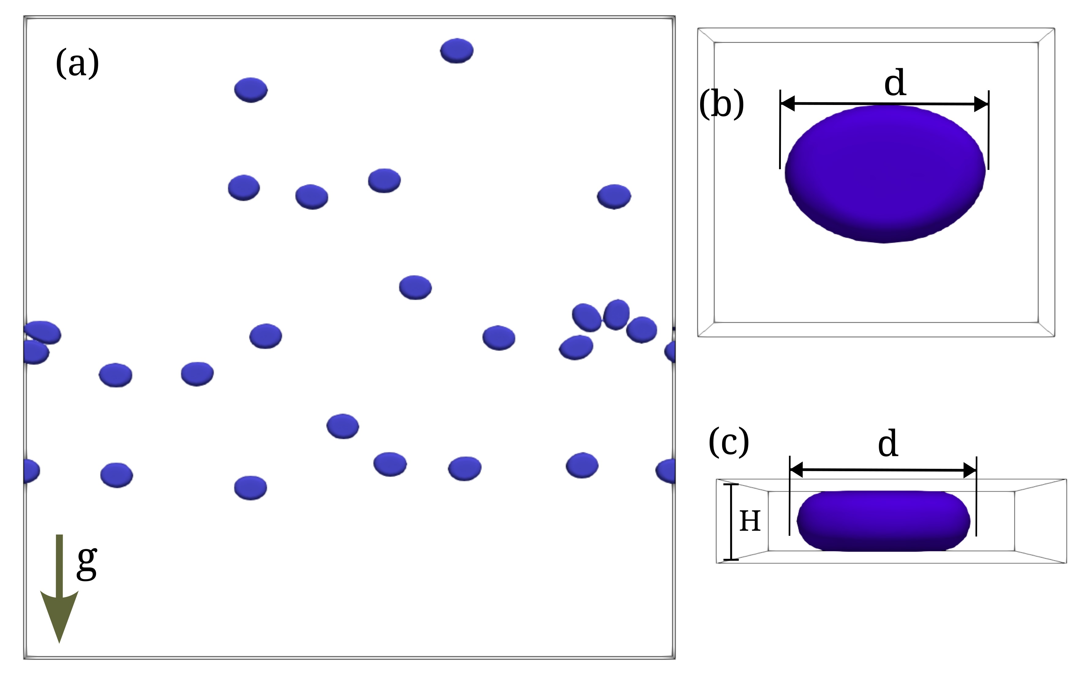
Figure 1: (a) Representative plot showing showing bubbles of diameter $d$ in a Hele-Shaw setup. The length along $x-$ and $z-$ directions is $L$, and the gap width in $y-$ direction is $H$; (b) Top view of a bubble (zoomed view); (c) Front view of the bubble (zoomed view).

3.1 Gap width averaged equations:

Experiments often use gap width averaged velocities to study statistical properties of the flow. Following the procedure outline in (Gondret and Rabaud, 1997; Alexakis and Biferale, 2018), and by assuming density $\rho$ to be constant along wall-normal direction, we get the following equations for the averaged in-plane horizontal components of the velocity:

$$(\partial_{t}+{\bf u}\cdot\nabla)\overline{c} = 0,~{}\rm{and}~{}\nabla\cdot{\bf u}=0,$$ (3)

$$\overline{\rho}(\partial_{t}+{\bf u}\cdot\nabla){\bf u} = -\overline{\rho}\nabla\cdot\overline{{\bf v}^{\prime}{\bf v}^{\prime}}+\nabla\cdot\left(2{{\mu}\mathbfsf{S}}\right)+\mathbf{\overline{F}}^{d}-\nabla\overline{P}+\mathbf{\overline{F}}^{g}+\mathbf{\overline{F}}^{\sigma}.$$ (4)

Here, $\overline{(.)}\equiv(1/H)\int_{0}^{H}(.)dy$ denotes gap averaging, $\nabla\equiv(\partial_{x},\partial_{z})$, ${\bf u}\equiv(u_{x}(x,z),u_{z}(x,z))$ is the gap averaged velocity field with $u_{x}=\overline{v}_{x}$, $u_{z}=\overline{v}_{z}$, ${\bf v}^{\prime}({\bf x})=(v_{x}-u_{x},v_{z}-u_{z})$ are the three-dimensional residual velocity fluctuations, $\overline{P}(x,z)$ is the gap-averaged pressure field, $\mathbfsf{S}=\nabla{{\bf u}}+\nabla{\bf u}^{T}$ is the gap-averaged strain-rate tensor, $\overline{\rho}(x,z)$ is the density field, ${\overline{\bf{F}}}^{g}=[\rho_{a}-\overline{\rho}]g\hat{z}$ is the buoyancy force, $\overline{\bf{F}}^{\sigma}$ is the surface tension force. The viscous dissipation contributes in two parts: (a) small-scale dissipation $\nabla\cdot\left(2\overline{{\mu}}\mathbfsf{S}\right)$, and (b) viscous drag due to walls ${\overline{\bf F}}^{d}=[\mu(\nabla{\bf v}+\nabla{\bf v}^{T})\cdot\hat{y}]^{H}_{0}$.

3.2 Numerical Method

We use a second-order finite-volume solver PARIS (Aniszewski et al., 2021) to simulate NSHS (Eq. (2)). For bubble tracking PARIS employs a front tracking method, and the time marching is performed either using the first order Euler method or the second order Crank-Nicolson method.

3.3 Initial conditions and parameters

We consider a cuboid of breadth $L_{y}=H$, and with equal length and height ($L_{x}=L_{z}=L$) [see Fig. 1]. We use periodic boundary conditions in the $x$ and $z$ directions, and impose no-slip velocity boundary ${\mathbf{u}}=0$ at the walls ($y=0$ and $y=H$). We place $N_{b}$ bubbles in random positions and initialize each one as an ellipsoid of volume $V=4.73\times 10^{3}$ (mono-disperse suspension). The bubbles are allowed to relax in the absence of gravity until they achieve the equilibrium pan-cake-like configuration (Ganesh et al., 2020) with diameter $d/H=2$. In table 1 we summarize the parameters used in our simulations.

Table 1: Parameters used in our simulations. We fix $L=512$, $H=12$, $N_{x}=N_{z}$, and $d=24$ for all the runs.

#	$N_{b}$	$N_{x}$	$N_{y}$	$\rho_{1}$	$\mu_{1}$	$\mu_{1}/\mu_{2}$	Ga	Bo	At	$\phi$
$\tt{H1}$	$24$	$1024$	$24$	$1.0$	$0.16$	$1$	$294$	$1.8$	$0.08$	$0.0552$
$\tt{H2}$	$46$	$512$	$32$	$1.0$	$0.16$	$1$	$294$	$1.8$	$0.08$	$0.1058$
$\tt{H3}$	$24$	$512$	$32$	$1.0$	$0.42$	$20$	$274$	$3.4$	$0.9$	$0.0552$

4 Results

In this section, we present the results of our numerical investigations. We monitor the time evolution of the gap-averaged energy and investigate the corresponding flow properties in a statistically steady state. The plot in Fig. 2 shows a typical snapshot of the bubble configuration along with the flow streamlines in the steady-state. Similar to the experiments (Bouche et al., 2014), we observe that the flow disturbances are mostly localized in the bubble vicinity. Furthermore, the horizontal alignment of bubbles is also observed in experiments (Bouche et al., 2014) as well as numerical simulation of stratified bubbly flows in a Hele-Shaw setup (Ganesh et al., 2020). As is conventional in the experiments (Bouche et al., 2012, 2014), we also investigate the spectral properties of the gap-averaged velocity field (4).

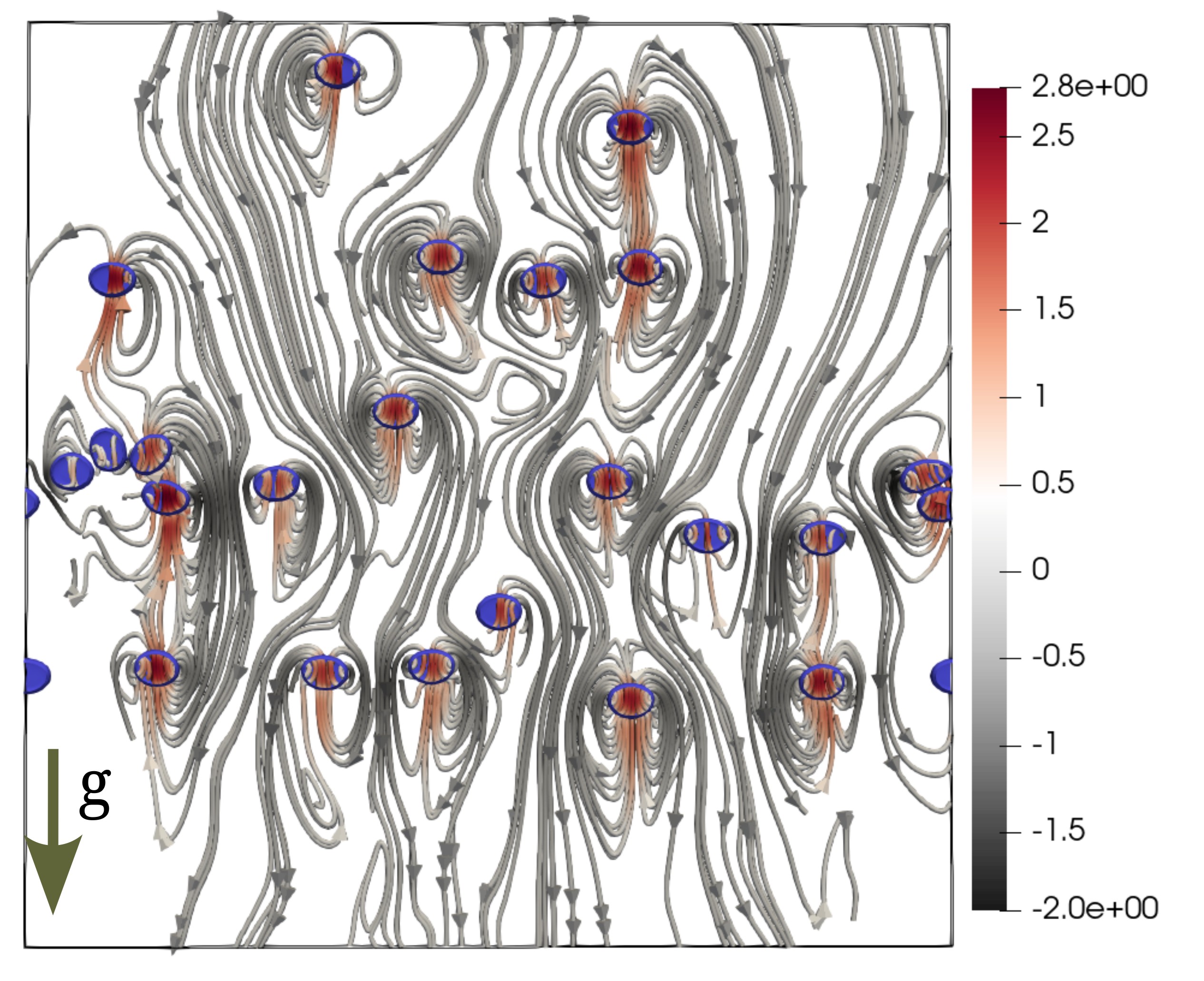
Figure 2: Instantaneous bubble configuration superimposed with flow streamlines in the steady-state (run ${\tt H1}$). The streamlines are colored according to the z-component of the velocity.

4.1 Time evolution

From (4), we obtain the following balance equation for the gap-averaged kinetic energy $E$

$$\partial_{t}\underbrace{\langle\frac{\overline{\rho}~{}{\bf u}^{2}}{2}\rangle}_{E}=-\underbrace{2\langle\overline{\mu}\mathscr{\mathbfsf{S}}:\mathscr{\mathbfsf{S}}\rangle}_{\epsilon_{\mu}}+\underbrace{\langle[\rho_{a}-\overline{\rho}]u_{z}g\rangle}_{\epsilon_{inj}}+\underbrace{\langle\mathbf{\overline{F}}^{\sigma}\cdot{\bf u}\rangle}_{\epsilon_{\sigma}}+\underbrace{\langle\mathbf{\overline{F}}^{d}\cdot{\bf u}\rangle}_{\epsilon_{d}},$$ (5)

where $\epsilon_{\mu}$ is the gap-averaged viscous energy dissipation, $\epsilon_{d}$ is the dissipation due to drag, $\epsilon_{inj}$ is the gap-averaged energy injected due to buoyancy, $\epsilon_{\sigma}$ is the contribution due to the surface tension, and the angular brackets denote spatial averaging.

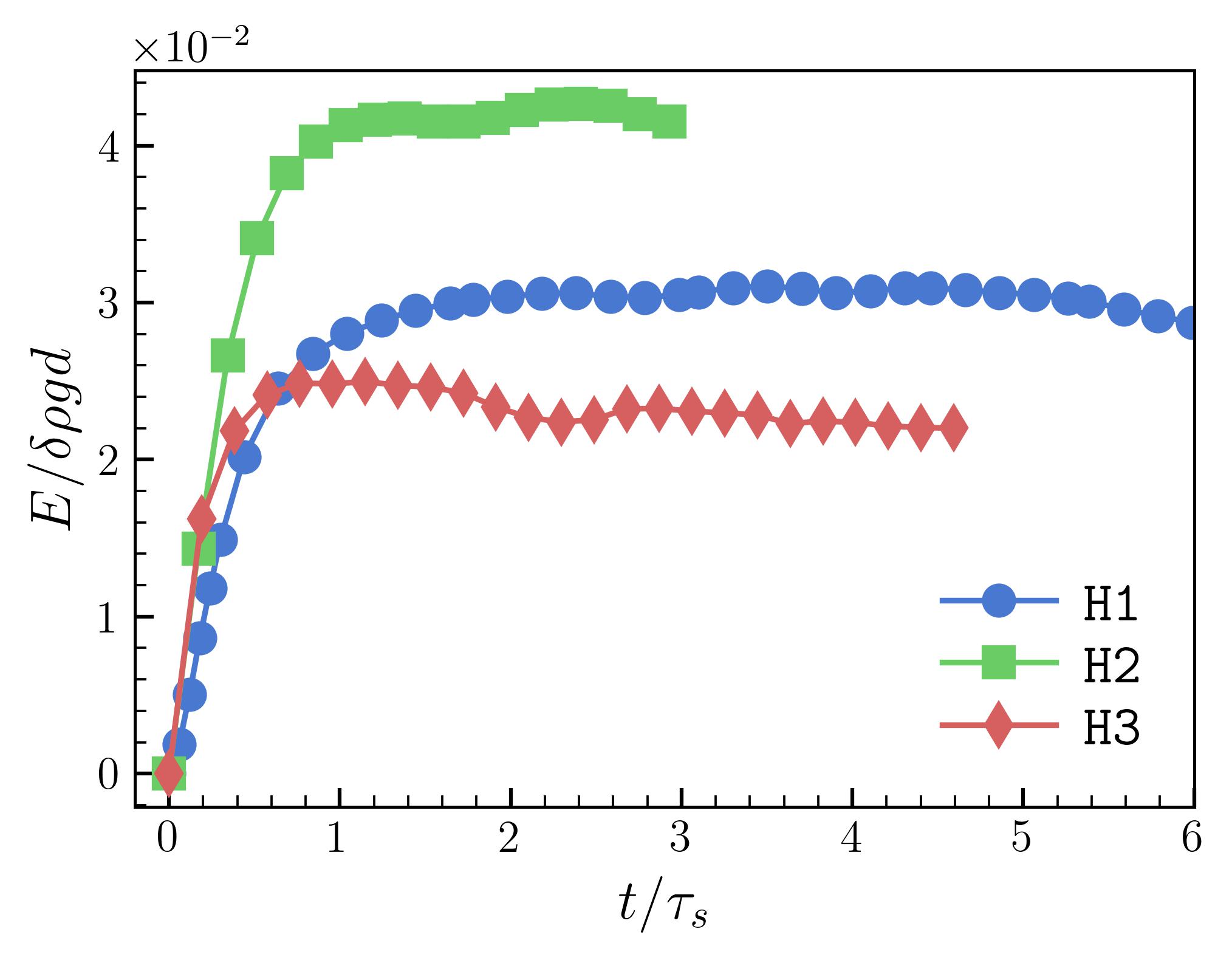
Figure 3: Time evolution of the kinetic energy $E$. A steady-state is attained for $t\geq 0.8\tau_{s}$, where $\tau_{s}=L/\sqrt{gd}$.

In Fig. 3, we plot the time-evolution of the kinetic energy $E$ and observe that a statistically steady state is achieved for $t>0.8\tau_{s}$. Furthermore, in table 2 we show that the energy injected by buoyancy is primarily balanced by the dissipation due to drag in the steady state ($\partial_{t}E\approx 0$).

Table 2: Time-averaged values of the energy injection $\epsilon_{inj}$, viscous dissipation $\epsilon_{\mu}$, and dissipation due to drag $\epsilon_{d}$ in the statistically steady state.

#	$\epsilon_{\mu}\times 10^{-3}$	$-\epsilon_{d}\times 10^{-3}$	$\epsilon_{inj}\times 10^{-3}$
$\tt{H1}$	$0.8$	$5.6$	$6.5$
$\tt{H2}$	$1.1$	$11.6$	$11.6$
$\tt{H3}$	$0.8$	$8.8$	$9.1$

4.2 Energy spectra and scale-by-scale energy budget

The energy spectrum and co-spectra for the gap-averaged velocity field are defined as:

$$E(k) \equiv \sum_{k-1/2<m<k+1/2}|\hat{\mathbf{u}}({\bf m})|^{2},$$

$$E^{\rho u}(k) \equiv \sum_{k-1/2<m<k+1/2}\Re[\hat{(\rho\mathbf{u})}({-\bf m})\hat{\mathbf{u}}({\bf m})].$$

Here, $\hat{(\cdot)}$ denotes the Fourier transformed fields.

In Fig. 4, we plot the energy spectra $E(k)$ and cospectra $E^{\rho u}(k)$ for our simulations ${\tt H1-H3}$ . From the plots, we can identify different scaling regimes: (a) For $k<<k_{d}$ we observe $E(k)\sim k$, where $k_{d}$ is the wavenumber corresponding to the bubble diameter; (b) Around $k\sim k_{d}$, we find a short $-3$ scaling regime followed by a steeper decay of the spectrum. Our simulations are also consistent with earlier experiments that also observe an intermediate $k^{-3}$ scaling subrange for $0.2\lessapprox k/k_{d}\lessapprox 1$ (Bouche et al., 2014).

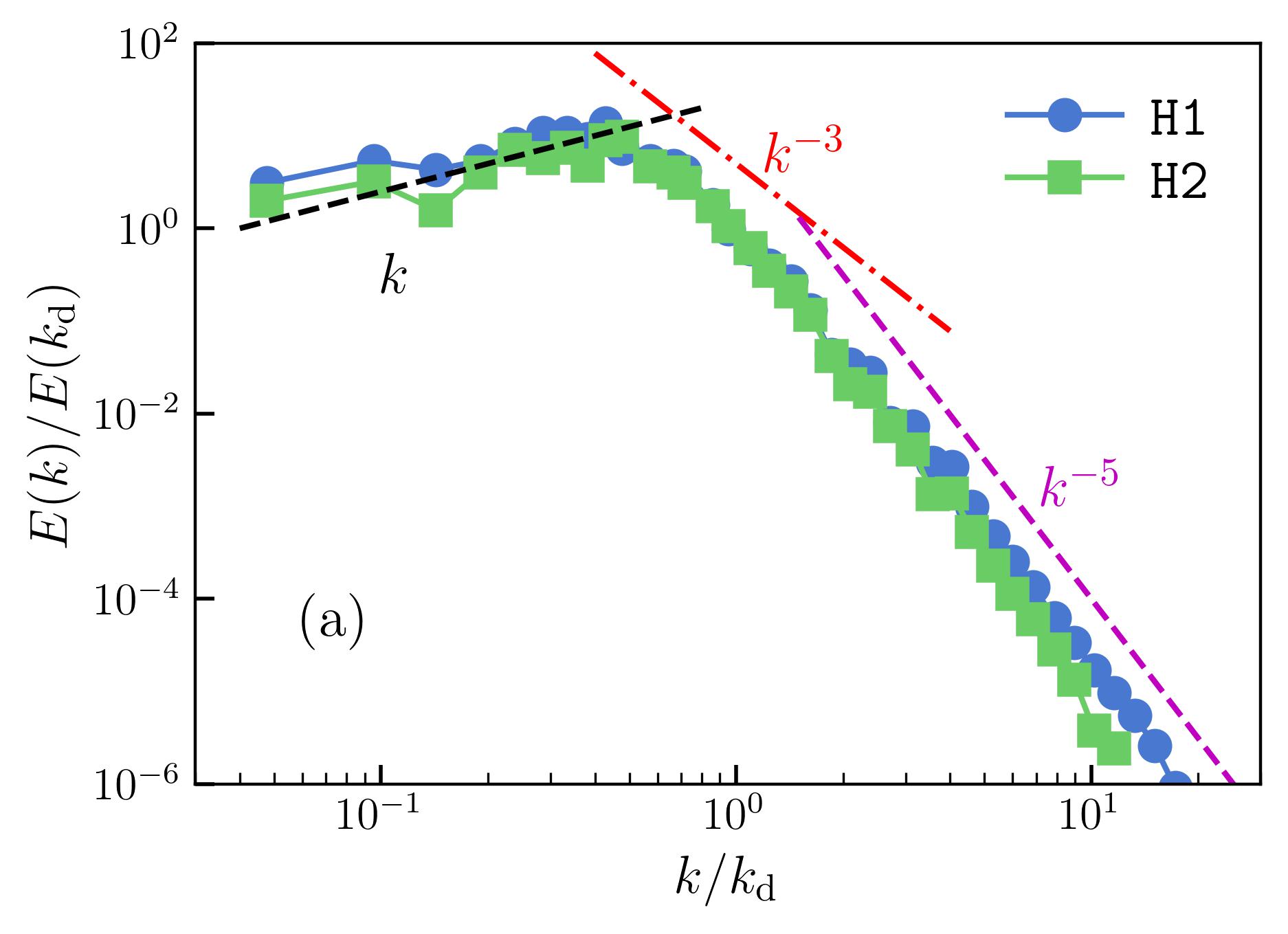
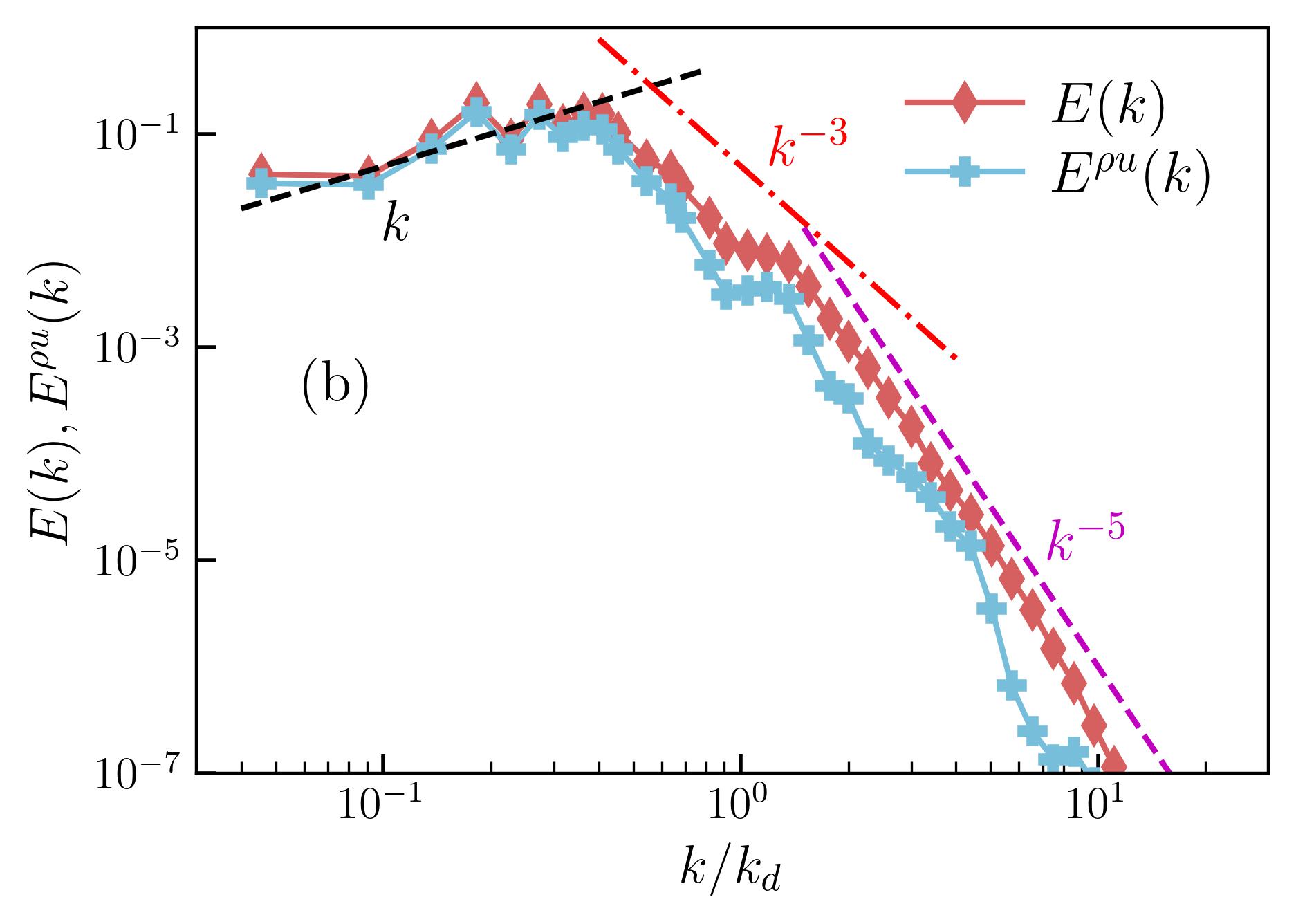
Figure 4: (a) Log-log of the energy spectra ($E(k)$ versus $k$) for low At runs ${\tt H1}$ and ${\tt H2}$. (b) Log-log plot of the energy spectra ($E(k)$) and cospectra ($E^{\rho u}(k)$) for high $\mbox{At}=0.9$ run $H3$ ($\mbox{Ga}=274$, $\phi=0.05$).

Risso (2011) argues that the $k^{-3}$ scaling could be modelled as a signal consisting of a sum of localized random bursts. Although this explanation is consistent with Fig. 2, it does not highlight the underlying mechanisms that generate the observed scaling. Lance and Bataille (1991) take an alternate viewpoint and argue that the balance of energy production and viscous dissipation leads to the $k^{-3}$ scaling.

The scaling of the energy spectrum we observe differs earlier studies on two-dimensional unbounded flows (Ramadugu et al., 2020; Innocenti et al., 2021) at comparable Ga. They find an inverse energy cascade with $E(k)\sim k^{-5/3}$ for $k<k_{d}$ and a $E(k)\sim k^{-3}$ scaling for $k>k_{d}$ due to the balance of energy injected by surface tension with viscous dissipation.

In what follows, we present an energy budget analysis to explain the observed scaling of the energy spectrum.

4.2.1 Energy budget

Since the scaling behaviour observed in our simulations ${\tt H1-H3}$ is identical, we perform the energy budget analysis using our highest resolution simulation ${\tt H1}$. Ignoring inertia and assuming a statistically steady state, from (4) we get the following energy budget equation (Verma, 2019; Pope, 2012):

$${\mathscr{F}}(k)+T^{\sigma}(k)=\underbrace{\nu k^{2}E(k)}_{D(k)}+\mathscr{D}(k),$$ (6)

where $T(k)$ is the nonlinear kinetic energy transfer, $D(k)$ is the viscous dissipation, $T^{\sigma}(k)=\sum^{\prime}\Re[\hat{\bf F}^{\sigma}({\bf m})\cdot\hat{{\bf u}}(-{\bf m})]$ is the nonlinear transfer due to surface tension, $\mathscr{D}(k)=-\sum^{\prime}\Re[\hat{\bf F}^{d}({\bf m})\cdot\hat{{\bf u}}(-{\bf m})]$ is the viscous dissipation due to drag, $\mathscr{F}(k)=\sum^{\prime}\Re[\hat{F}^{g}({\bf m})\hat{u}_{z}(-{\bf m})]$ is the energy injection due to buoyancy. Here, $\sum^{\prime}\equiv\sum_{|{\bf m}|<{k-1/2}}^{k+1/2}$ indicates summation over all wave-numbers in a circular shell around wavenumber $k$.

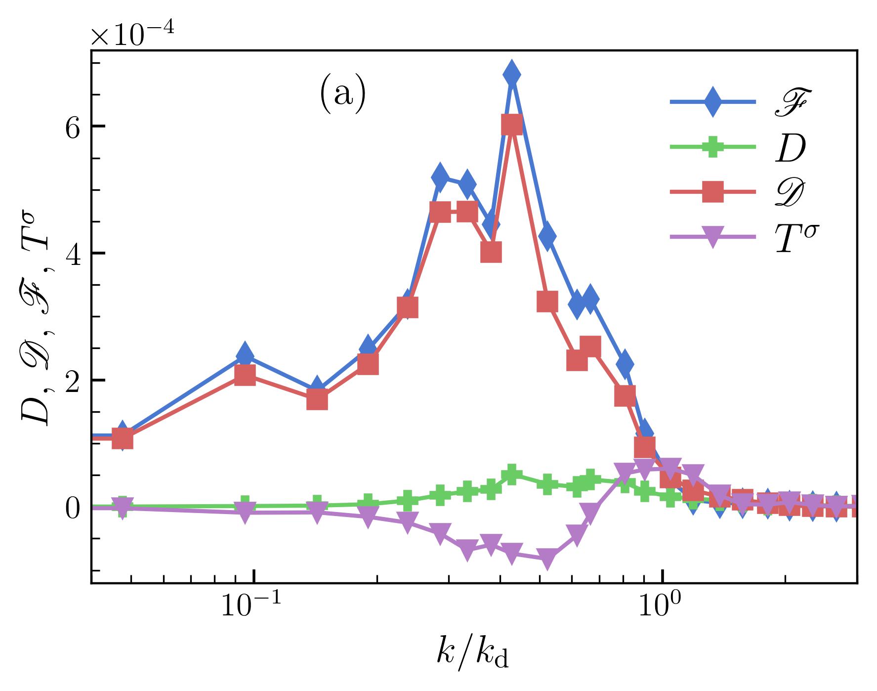
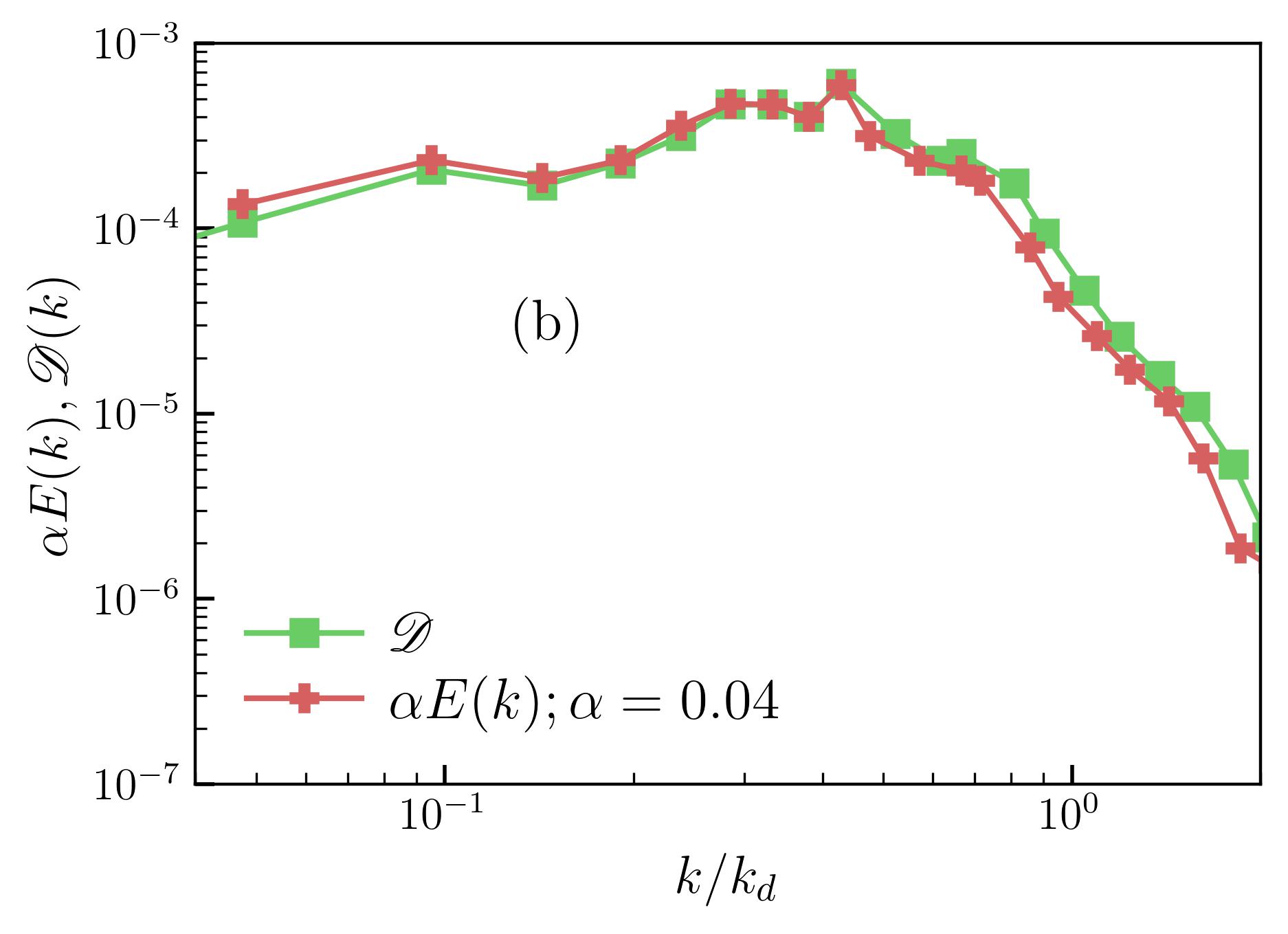
Figure 5: (a) Lin-log plot of the different contributions to the spectral energy budget (6) obtained from run ${\tt H1}$. (b) Log-log plot showing comparison of the scaled energy spectrum $\alpha E(k)$ and the dissipation due to drag ${\mathscr{D}}$(k) for $k/k_{d}<2$.

The plot in Fig. 5(a) shows the different contributions to the budget. Clearly for $k<k_{d}$, the energy injected by buoyancy is balanced by the drag ($F^{g}(k)\sim\mathscr{D}(k)$) and other contributions are subdominant. This justifies our assumption of ignoring the inertial terms. In Fig. 5(b), we show that a linear drag approximation $F^{d}(k)\sim\alpha E(k)$ (with $\alpha=0.04$) is in excellent agreement with ${\mathscr{D}}(k)$. Next we approximate the energy injected by buoyancy as $F^{g}(k)\sim\sqrt{E(k)E_{\rho}(k)}$, where $E_{\rho}(k)=\sum^{\prime}|\hat{\rho}({\bf m})|^{2}$. Noting that for $k<<k_{d}$, i.e. for scales much larger than bubble size, the density field can be approximated by white noise $E_{\rho}(k)\sim k$ and by balancing the energy injected by buoyancy with drag, we obtain $E(k)\sim k$. This explains the scaling observed in our simulations for $k<k_{d}$.

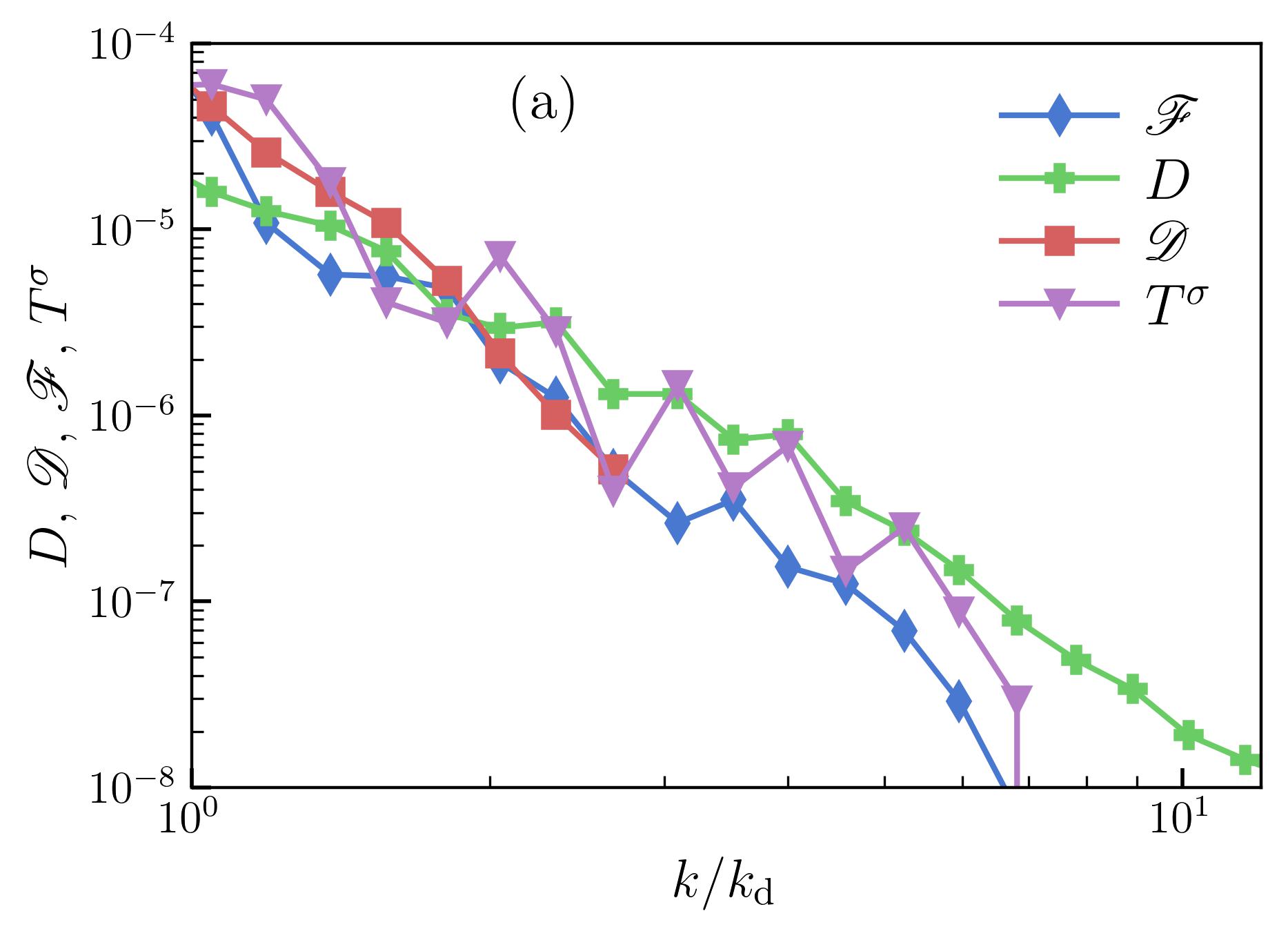
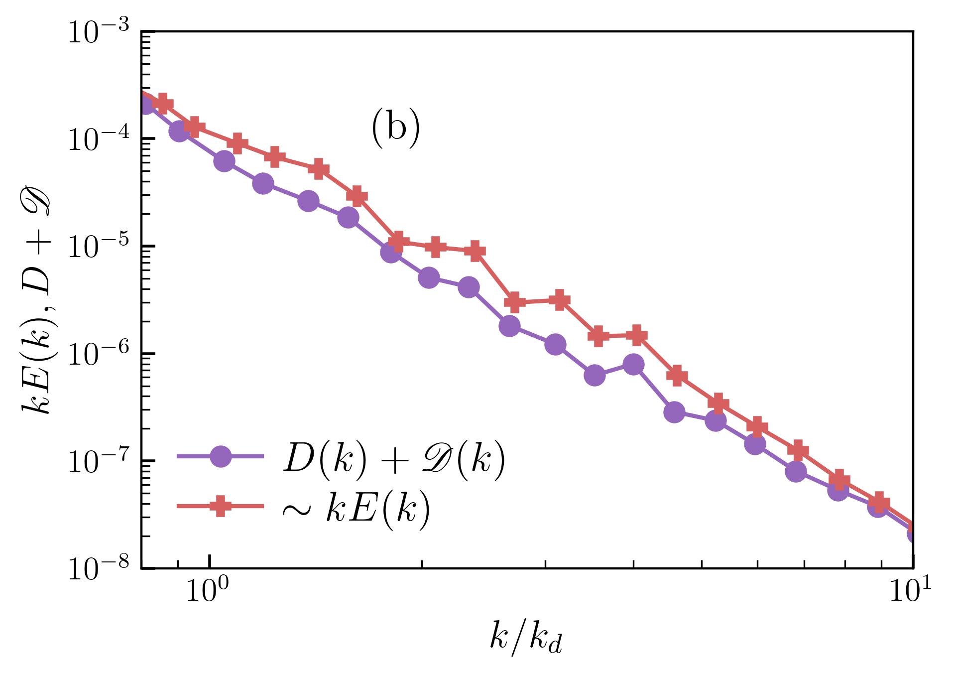
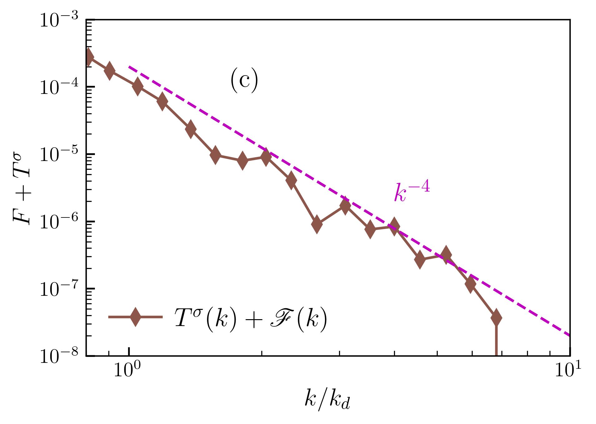
Figure 6: (a) Zoomed in plot showing contributions to the spectral energy budget for $k>k_{d}$. (b) Log-log plot showing comparison of the scaled dissipation spectrum $\sim kE(k)$ and the net dissipation $D(k)+{\mathscr{D}}(k)$ for $k>k_{d}$. (c) Log-log plot showing different scaling regimes in the net energy injection ${\mathscr{F}}(k)+T^{\sigma}(k)$ for $k>k_{d}$.

The situation is more complicated for $k>k_{d}$. The zoomed-in plot of the energy balance (see Fig. 6(a)) reveals that both buoyancy and the surface tension inject energy that gets dissipated by the viscous forces ($D+\mathscr{D}$), and there is no dominant balance ($\mathscr{F}+T^{\sigma}\sim D+\mathscr{D}$). In Fig. 6(b), we show that the net dissipation $D+{\mathscr{D}}\sim kE(k)$. Similarly, the net production $\mathscr{F}+T^{\sigma}\sim k^{-4}$ for $k>k_{d}$. Therefore, by balancing the net injection with dissipation we get $E(k)\sim k^{-5}$ scaling for $k>k_{d}$. Given the limited cross-over scaling range $E(k)\sim k^{-3}$ in Fig. 4, we are unable to argue about the underlying mechanisms. Thus the plausible explanation for the $-3$ scaling is the argument by Risso (2011) that we have discussed in the previous section.

4.3 Two-dimensional Navier-Stokes equations with a linear drag (NSD)

In this section we investigate whether two-dimensional Navier-Stokes with a linear drag coefficient (8) is able to model the confined bubbly flows. In the following, we assume all the fields are two-dimensional and for comparison with the gap-averaged quantities, we choose the same symbols.

$$D_{t}c = 0,~{}\rm{and}~{}\nabla\cdot{{\bf u}}=0,$$ (7)

$$\rho(c)D_{t}\mathbf{u} = \nabla\cdot\left[2\mu(c)\mathbfsf{S}\right]-\nabla P+{\bf F}^{g}+{\bf F}^{\sigma}-\alpha{\bf u}.$$ (8)

We perform the NSD simulations with a square domain of area $L^{2}$ and discretize it with $2048^{2}$ equi-spaced points. The bubbles are initialized as circles of diameter $d=24$ and all the parameters of the simulation are identical to our run ${\tt H1}$ and we fix the drag coefficient $\alpha=0.04$. Our choice for the value of $\alpha$ is motivated by Fig. 5. We use a front-tracking-pseudo-spectral method to evolve (8). For details of the numerical scheme, we refer the reader to Ramadugu et al. (2020). Below we discuss the statistical properties of the flow in the steady state.

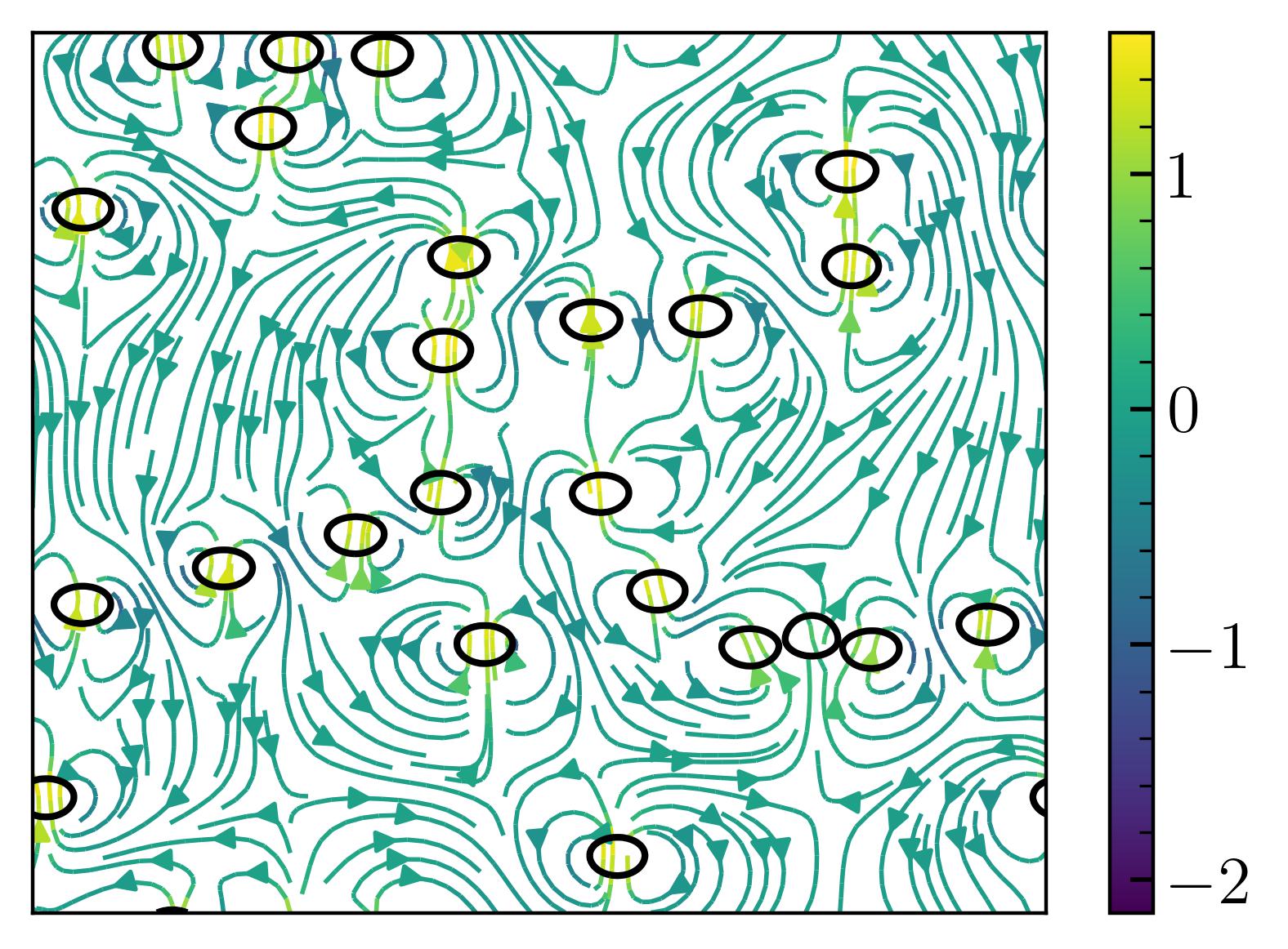
Figure 7: (a) Snapshot of the bubble positions overlaid with flow streamlines. (b) Comparison of the gap-averaged energy spectra for our NSHS run ${\tt H1}$ with the energy spectra obtained using simulation of the NSD equation (8).

In Fig. 7(a), we plot the bubble configuration and the flow streamlines. Clearly the large scale flow properties resemble those observed for the NSHS simulation. The flow disturbances are localized in the vicinity of the bubbles and we also observe horizontal alignment of bubbles.

The plot in Fig. 7(b) shows a comparison of the gap-averaged energy spectrum $E(k)$ obtained from the NSHS equation with that obtained from NSD equation (8). We find that the energy spectrum are nearly identical for $k<k_{d}$, $E(k)\sim k$. However, discrepancies are observed for $k>k_{d}$, in contrast to $E(k)\sim k^{-5}$ for the NSHS simulations we find $E(k)\sim k^{-3}$ for the NSD simulations.

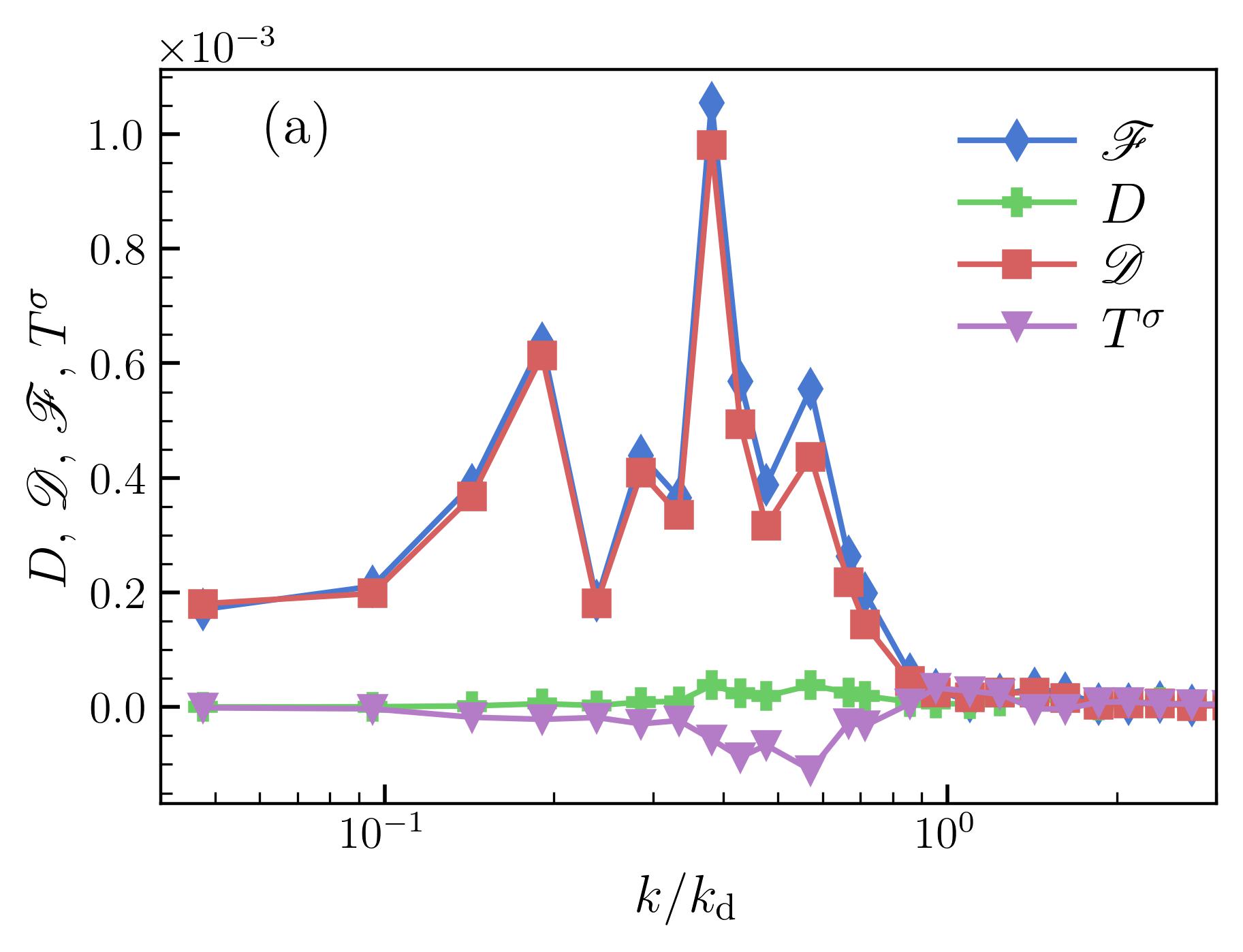
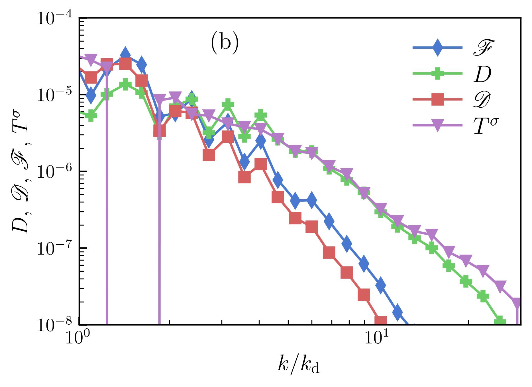
Figure 8: Different contributions towards the energy budget for (a) $k<k_{d}$ and (b) $k>k_{d}$ obtained from NSD simulation.

Using (8), and ignoring the inertial contributions, we obtain the following energy balance

$${\mathscr{F}}(k)+T^{\sigma}(k)=\underbrace{\nu k^{2}E(k)}_{\mathscr{D}}+\underbrace{\alpha E(k)}_{D}.$$ (9)

In Fig. 8, we plot the contribution of different terms in (9) towards energy balance. For $k<k_{d}$, similar to NSHS, we observe that energy injected by buoyancy is balanced by the linear drag. However, a different balance appears for $k>k_{d}$. In contrast to NSHS, a dominant balance is observed in the NSD equations. The energy transfer by surface tension to small scales balances viscous dissipation leading to the observed $E(k)\sim k^{-3}$ scaling in the energy spectrum. Similar small-scale balance has also been reported in earlier two-dimensional unbounded bubbly flow simulations (Ramadugu et al., 2020).

Therefore, we conclude that although the NSD model captures the large scale dynamics of the Hele-Shaw flow (NSHS), it is unable to correctly capture the small scale physics.

5 Conclusion

We have investigated the spectral properties of the two-dimensional bubbly flows under confinement in a Hele-Shaw setup for experimentally relevant Ga and $\phi$. The flow visualization in the steady state is similar to earlier experimental observations (Bouche et al., 2014). The energy spectrum obtained from the gap-averaged velocity field shows $E(k)\sim k$ for $k<k_{d}$ and $E(k)\sim k^{-5}$ for $k>k_{d}$. We also observe an intermediate scaling range with $E(k)\sim k^{-3}$ around $k\sim k_{d}$. A scale-by-scale energy budget analysis reveals the dominant balances. For $k<k_{d}$, energy injection balances dissipation due to drag, whereas for $k>k_{d}$, the net injection balances net dissipation. Finally, we show that the Navier-Stokes equation with a linear drag can be used to approximate large scale flow properties of bubbly Hele-Shaw flow but it fails to correctly capture energy balance at scales smaller than the bubble diameter.

Conflict of Interest Statement

The authors declare that the research was conducted in the absence of any commercial or financial relationships that could be construed as a potential conflict of interest.

Author Contributions

P.P contributed to conception and design of the study. R.R. and V.P. contributed equally. R.R. performed initial NSHS and NSD simulations. V.P. performed NSHS simulations. V.P. and P.P. performed the analysis and wrote the manuscript. All authors read, and approved the submitted version.

Funding

We acknowledge support from the Department of Atomic Energy (DAE), India under Project Identification No. RTI 4007, and DST (India) Project Nos. ECR/2018/001135 and DST/NSM/R&D_HPC_Applications/2021/29.

References

- Alexakis and Biferale (2018) Alexakis, A. and Biferale, L. (2018). Cascades and transitions in turbulent flows. Phys. Rep. 767, 1–101
- Aniszewski et al. (2021) Aniszewski, W., Arrufat, T., Crialesi-Esposito, M., Dabiri, S., Fuster, D., Ling, Y., et al. (2021). Parallel, robust, interface simulator (paris). Comp. Phys. Communications 263, 107849
- Bouche et al. (2012) Bouche, E., Roig, V., Risso, F., and Billet, A. (2012). Homogeneous swarm of high-reynolds-number bubbles rising within a thin gap. part 1. bubble dynamics. J. Fluid. Mech. 704, 211–231
- Bouche et al. (2014) Bouche, E., Roig, V., Risso, F., and Billet, A. (2014). Homogeneous swarm of high-reynolds-number bubbles rising within a thin gap. part 2. liquid dynamics. J. Fluid. Mech. 758, 508–521
- Brackbill et al. (1992) Brackbill, J. U., Kothe, D. B., and Zemach, C. (1992). A continuum method for modeling surface tension. J. Comput. Phys. 100, 335 – 354
- Clift et al. (1978) Clift, R., Grace, J. R., and Weber, M. E. (1978). Bubbles, drops and particles (Academic Press, New York)
- Filella et al. (2015) Filella, A., Patricia, E., and Roig, V. (2015). Oscillatory motion and wake of a bubble rising in a thin-gap cell. J. Fluid Mech. 778, 60–88
- Ganesh et al. (2020) Ganesh, M., Kim, S., and Dabiri, S. (2020). Induced mixing in stratified fluids by rising bubbles in a thin gap. Phys. Rev. Fluids 5, 043601
- Gondret and Rabaud (1997) Gondret, P. and Rabaud, M. (1997). Shear instability of two-fluid parallel flow in a hele–shaw cell. Physics of Fluids 9, 3267–3274
- Innocenti et al. (2021) Innocenti, A., Jaccod, A., Popinet, S., and Chibbaro, S. (2021). Direct numerical simulation of bubble-induced turbulence. Journal of Fluid Mechanics 918
- Kelley and Wu (1997) Kelley, E. and Wu, M. (1997). Path instabilities of rising air bubbles in a hele-shaw cell. Physical review letters 79, 1265
- Lance and Bataille (1991) Lance, M. and Bataille, J. (1991). Turbulence in the liquid phase of a uniform bubbly air–water flow. Journal of Fluid Mechanics 222, 95–118
- Mathai et al. (2020) Mathai, V., Lohse, D., and Sun, C. (2020). Bubble and buoyant particle laden turbulent flows. Annu. Rev. Condens. Matter Phys. 11, 529
- Mendez-Diaz et al. (2013) Mendez-Diaz, S., Serrano-Garcia, J. C., Zenit, R., and Hernández-Cordero, J. A. (2013). Power spectral distributions of pseudo-turbulent bubbly flows. Phys. Fluids 25, 043303
- Mudde (2005) Mudde, R. F. (2005). Gravity-driven bubbly flows. Annu. Rev. Fluid Mech. 37, 393–423
- Pandey et al. (2022) Pandey, V., Mitra, D., and Perlekar, P. (2022). Turbulence modulation in buoyancy-driven bubbly flows. Journal of Fluid Mechanics 932, A19. 10.1017/jfm.2021.942
- Pandey et al. (2020) Pandey, V., Ramadugu, R., and Perlekar, P. (2020). Liquid velocity fluctuations and energy spectra in three-dimensional buoyancy-driven bubbly flows. J. Fluid Mech. 884, R6
- Pope (2012) Pope, S. (2012). Turbulent Flows (Cambridge University Press)
- Prakash et al. (2016) Prakash, V. N., Mercado, J. M., van Wijngaarden, L., Mancilla, E., Tagawa, Y., Lohse, D., et al. (2016). Energy spectra in turbulent bubbly flows. J. Fluid Mech. 791, 174–190
- Ramadugu et al. (2020) Ramadugu, R., Pandey, V., and Perlekar, P. (2020). Pseudo-turbulence in two-dimensional buoyancy-driven bubbly flows: a dns study. The European Physical Journal E 43, 1–8
- Riboux et al. (2010) Riboux, G., Risso, F., and Legendre, D. (2010). Experimental characterization of the agitation generated by bubbles rising at high reynolds number. J. Fluid Mech. 643, 509–539
- Risso (2011) Risso, F. (2011). Theoretical model for psectra in dispersed multiphase flows. Phys. Fluids 23, 011701
- Risso (2018) Risso, F. (2018). Agitation, mixing, and transfers induced by bubbles. Annu. Rev. Fluid Mech. 50, 25
- Roig et al. (2012) Roig, V., Roudet, M., Risso, F., and Billet, A.-M. (2012). Dynamics of a high-reynolds-number bubble rising within a thin gap. J. Fluid Mech. 707, 444–466
- Verma (2019) Verma, M. (2019). Energy transfers in fluid flows (Cambridge University Press)
- Wang et al. (2014) Wang, X., Klaasen, B., Degrève, J., Blanpain, B., and Verhaeghe, F. (2014). Experimental and numerical study of buoyancy-driven single bubble dynamics in a vertical hele-shaw cell. Phys. Fluids 26, 123303