Understanding stock market instability via graph auto-encoders

Abstract

Understanding stock market instability is a key question in financial management as practitioners seek to forecast breakdowns in asset co-movements which expose portfolios to rapid and devastating collapses in value. The structure of these co-movements can be described as a graph where companies are represented by nodes and edges capture correlations between their price movements. Learning a timely indicator of co-movement breakdowns (manifested as modifications in the graph structure) is central in understanding both financial stability and volatility forecasting. We propose to use the edge reconstruction accuracy of a graph auto-encoder (GAE) as an indicator for how spatially homogeneous connections between assets are, which, based on financial network literature, we use as a proxy to infer market volatility. Our experiments on the S&P 500 over the 2015-2022 period show that higher GAE reconstruction error values are correlated with higher volatility. We also show that out-of-sample autoregressive modeling of volatility is improved by the addition of the proposed measure. Our paper contributes to the literature of machine learning in finance particularly in the context of understanding stock market instability.

Keywords
Graph Based Learning, Graph Neural Networks, Graph Autoencoder, Stock Market Information, Volatility Forecasting

1 Introduction

Financial market instability has long interested investors, as, during financial collapses, previously uncorrelated companies collapse in value together, which exposes the market to a systemic level of risk that goes beyond the level of the company and requires a more global outlook (Andersen et al., , 2006). Understanding this market-wide systemic risk driven by asset co-movement requires framing connections between firms as formed by evolving ‘complex adaptive networks’ (Haldane, , 2009). This turns instability detection into a network analysis task. These networks are usually constructed by transforming and filtering correlation matrices of price returns (Mantegna, , 1999). They capture key structures of the correlation matrices, and, at the same time they avoid potentially noisy features derived from correlations directly (Serur and Avellaneda, , 2021). Topological features of the resulting financial graphs, such as shorter diameters (Mantegna, , 1999), higher cluster density (Mantegna, , 1999; Onnela et al., , 2004; Tumminello et al., , 2010), or lower Ricci curvature (Samal et al., , 2021; Sandhu et al., , 2016), are shown to be positively linked to market instability measures such as higher volatility.

This suggests that higher market instability results from breakdowns to previously homogeneous patterns of network connectivity. Homogeneity is defined here as regular connection patterns across the entire network Xue et al., (2022). In financial networks, homogeneous patterns are connections between companies of the same industry sectors and with similar returns (Kukreti et al., , 2020). Homogeneity-disturbing shocks arise from news announcements about financial events or asset bubbles and affect the ways in which the assets co-move by modifying the way investors form opinions about how companies are related and how they will co-evolve (Campbell et al., , 2002; Lim et al., , 2020; Preis et al., , 2012). From this perspective, market instability can be seen as modifying the underlying mechanism through which inter-company connectivity structures appear. Kukreti et al., (2020) points out that heterogeneously connected graphs indicates higher instability, as any shock could travel further across the entire market and not be limited to a single sector (Artzner et al., , 1999; Das et al., , 2019). Heterogeneity in a network is defined as difference over all pairs of linked nodes of a function applied to node features Estrada, (2010). Heterogeneous market networks are therefore characterised by high connectivity between companies which differ in industry sector, market capitalisation or long-run returns. Increase in this heterogeneity has been shown to granger-cause increases in the VIX volatility index Zhao et al., (2016). Conversely, more homogeneous periods when strong connections only exist between similar assets would indicate lower risk, as any shock would propagate at most throughout that asset’s immediate neighbourhood in the financial graph and not the entire market (Samal et al., , 2021; Heiberger, , 2014).

However, the “network-only” approaches mentioned above may not fully capture homogeneity of connections between different types of nodes. Indeed, once networks are constructed, they do not make further use of any form of node features. This means they implicitly assume that all information about company nodes is captured by their connectivity. This discount information from the underlying price returns which traditional volatility forecasting models like multivariate GARCH (Chandra, , 2003) or HEAVY (Noureldin et al., , 2012) successfully use in forecasting volatility. Thus, a measure which accounts for both the network and node features is lacking. This leads to the open question of how to measure market instability using financial networks with company characteristics such as returns.

The graph machine learning literature has provided tools for the joint learning of these features (Chami et al., , 2022). However, their applications to financial graphs remain mostly limited to return forecasting, with very few works looking at volatility forecasting directly (Saha et al., , 2022). Wang et al., (2022) point to the lack of unsupervised models in graph neural network applications to the stock market that can learn representations of market states instead of only directly forecasting them. We propose a graph auto-encoder (GAE) (Kipf and Welling, , 2016) to capture both connectivity and node feature information as part of an edge reconstruction task. Good GAE performance would indicate good node embeddings and a more stable and homogeneous market as homogeneity in edge connectivity helps reconstruction performance. Assuming the GAE is well trained, it should be able to group companies of similar returns together. If, once trained, the GAE performs poorly in reconstructing structures of financial graphs of future time steps, we argue this indicates a shift in the way connections are formed in the future graph. We interpret this shift as an increased instability in the financial network. Indeed, if the GAE performs worse, then the future graph has heterogeneous connections between companies of different returns and different sectors. A worse reconstruction performance then reflects the definition of a non-homogeneous, unstable graph from literature Kukreti et al., (2020); Onnela et al., (2004); Xue et al., (2022).

2 Problem setting and methodology

2.1 Problem setting

Consider a financial network represented by a graph $\mathcal{G}=\{\mathcal{E},\mathcal{V}\}$, with nodes representing firms and edges the similarities or correlations between firm prices. In addition, consider a matrix $\mathbf{X}$ where the $u$-th column of $\mathbf{X}^{T}$, $\mathbf{x}_{u}$, is a vector of features that characterise the firm $u$ (e.g., its stock prices at given time intervals). Our goal is to develop a measure of the instability of the financial market given $\mathcal{G}$ and $\mathbf{X}$.

Recent works have analysed market instability by investigating the connectivity of $\mathcal{G}$ alone (Onnela et al., , 2004; Samal et al., , 2021). To take into account further information in $\mathbf{X}$, we utilise the GAE proposed in (Kipf and Welling, , 2016) which learns vector representations of nodes using both $\mathcal{G}$ and $\mathbf{X}$. The auto-encoder is trained on an edge reconstruction task described in Sec. 2.3 where we use a random subset of edges for training and the remaining edges for testing. A good performance on this task would indicate a more homogeneous pattern of edge formation across the graph.

With this understanding, we frame the problem of measuring market instability as one that quantifies heterogeneity in connectivity patterns between different areas of $\mathcal{G}$. As shown in Kukreti et al., (2020), homogeneous connectivity patterns are usually observed in low volatility periods where companies in related sectors are often exposed to similar fluctuations and overall more connected to each other than to companies outside their industries. On the other hand, more volatile markets are characterised by highly perturbed correlation structures leading to areas of the graph with highly different connectivity patterns. We therefore treat the generalisation ability of the edge reconstruction task above as a proxy for market instability. A high reconstruction performance on average with a randomly chosen split of training and test sets would indicate more stable market, while a low performance suggests the opposite due to heterogeneous connectivity patterns across the graph.

2.2 Data

We provide a practical context of the problem described above. Our data set consists of 6 years of stock market price data for stocks in the S&P 500 at the minute-level frequency from 2015 to 2021. From these price movements which we define as $p(n,t)$ where where the $nt$-th entry is the price for company $n$ at $t$, we calculate a log return matrix $\mathbf{X}\in\mathbb{R}^{N\times T}$ of $N$ companies over $T$ time periods at frequency $\Delta t$ :

$$r(t,n)=\text{log}(p(t,n))-\text{log}(p(t-\Delta t,n))$$ (1)

Based on this return matrix, we calculate a Pearson correlation matrix based on a rolling window of length $S$ days. This correlation matrix measures for all stock return pairs the covariance normalised by the square root of the product of the variances. It represents the strength of linear relationships between all the stock pairs. Given a return matrix of of $N$ companies over $T$, this gives us $T-S$ correlation matrices in total. Following Kukreti et al., (2020), we define an adjacency matrix $\mathbf{A}$ as $\mathbf{A}_{uv}=1$ if the ($u,v$) return pair has a correlation higher than 0.7 and otherwise we set $\mathbf{A}_{uv}$ to 0. The 0.7 threshold is selected to only keep strongly connected pairs and discount correlations of insufficient strengths Caccioli et al., (2018)Kukreti et al., (2020).

We calculate the return volatility (RV) that is used throughout the following sections as a proxy for instability according to the formula set out in Eq. (2). It is a measure of the variance of the returns of the average price returns over $\Delta t$ periods:

$$\text{RV}_{t}^{t+\Delta t}=\sum_{t}^{t+\Delta t}(r(t,n)^{2})$$ (2)

Because of the power law distribution of market volatility with orders of magnitude larger swings on high-volatility days, volatility is often measured as the natural logarithm of RV and termed log-RV.

We summarise the way we construct the financial network in Fig. (1) where a series of stock prices is transformed into a return matrix. From those returns, we calculate the correlation matrix as described above. Lastly, through a threshold applied to that correlation matrix, we obtain a network of connected companies.

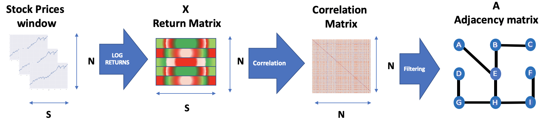
Figure 1: Pipeline generating networks from N returns over a window of time S

2.3 Proposed methodology

Based on the problem setting and data description in the previous two sections, we now formally describe our methodology. Given the financial graph $\mathcal{G}$ with adjacency matrix $\mathbf{A}$ and node features $\mathbf{X}$ defined above, we propose to use the GAE (Kipf and Welling, , 2016) as the edge reconstruction model whose generalisation ability is used to approximate market instability.

The GAE is an unsupervised representation learning model with an encoder and a decoder. The encoder is a function defined in Eq. (3). It describes an operation mapping the input $\mathbf{X}$ to the latent embedding $\mathbf{Z}$ via a 2-layer graph convolutional network (GCN) encoder (Kipf and Welling, , 2017). Once the encoder generates the embedding $\mathbf{Z}$, the decoder in equation Eq. (4) aims to reconstruct the edges present in the initial adjacency matrix. The embedding $\mathbf{Z}$ is of “good quality” if the reconstruction $\mathbf{\hat{A}}$ is close to the initial adjacency matrix. The GAE is trained by minimising a binary cross-entropy (BCE) loss defined in Eq. (5) on training edges $\mathbf{A}_{uv}$:

$$\mathbf{Z}=\text{GCN}(\mathbf{A},\mathbf{X})=\mathbf{\tilde{A}}*\text{ReLU}(\mathbf{\tilde{A}}*\mathbf{X}*\mathbf{W_{0}})*\mathbf{W_{1}}$$ (3)

$$\forall(u,v)\in\mathcal{V}*\mathcal{V},\mathbf{\hat{A}}=\sigma(\mathbf{z_{u}}*\mathbf{z_{v}})=\frac{1}{(1+e^{-\mathbf{z_{u}}*\mathbf{z_{v}}})}$$ (4)

$$(\mathbf{A}_{uv},\mathbf{\hat{A}}_{uv})=-\mathbf{A}_{uv}*log(\mathbf{\hat{A}}_{uv})-(1-\mathbf{A}_{uv})*log(1-\mathbf{\hat{A}}_{uv})$$ (5)

With the following definitions :

• $\mathbf{\tilde{A}}=\mathbf{D}^{-\frac{1}{2}}\mathbf{A}\mathbf{D}^{-\frac{1}{2}}$ is the normalised adjacency matrix of the graph. Where $\mathbf{D}=diag(d)$ is the diagonal matrix of the graph $\mathcal{G}$ where the values on the diagonal correspond to the degree of the node.

• ReLU($\mathbf{x}$) = max($\mathbf{x}$,0) is the non-linear activation function of the GCN.

• $\mathbf{W_{0}}$ and $\mathbf{W_{1}}$ are learnable weight matrices

The end-to-end training is done using gradient descent for which we selected a standard Adam algorithm (Kingma and Ba, , 2015). Fig. 2 below summarises how the GAE operates.

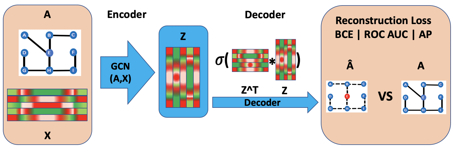
Figure 2: Summary of GAE operations

We now describe how we make use of the GAE model to derive a measure of market instability. We first extract the returns data $\mathbf{X}$ from a window of length $S=20$ days. From those returns, we generate the corresponding market graph $\mathcal{G}_{t}$ with $t$ denoting the last day in the time window using the methodology described in 2.2. We selected a span of 20 days as this represents one month of trading data, which is long enough to capture relations between companies without too much noise from unstable correlations in shorter windows Kukreti et al., (2020). Shifting the window by one day, we generate the next day market graph $\mathcal{G}_{t+1}$.

We trained and validated the GAE on $\mathcal{G}_{t}$, and test its performance by applying the trained model to reconstruct edges in $\mathcal{G}_{t+1}$, the market graph of next day $t+1$. We assume the GAE is trained on a period of stable market, which means a graph with spatially homogeneous connectivity structures. Following the reasoning in Section 2.1, once a GAE is trained, it can reconstruct the adjacency matrix of an unobserved graph in proportion to how spatially homogeneous the unobserved graph is Kipf and Welling, (2016). Consequently, any drop of the GAE testing accuracy on $\mathcal{G}_{t+1}$ can be viewed as an increase in graph heterogeneity. This increased heterogeneity measures how different the edge formation mechanism in $\mathcal{G}_{t+1}$ is different from $\mathcal{G}_{t}$. Previous results in the literature, such as Zhao et al., (2016) suggest that the change in market network homogeneity, measured by edit distance of edges between two successive time periods, granger-causes increases in market volatility. Following that approach, we interpret the difference in edge formation mechanism between $\mathcal{G}_{t}$ and $\mathcal{G}_{t+1}$ as resulting from shocks to investor opinion which push the market towards a more volatile state Lim et al., (2020); Preis et al., (2012). These shocks also form the basis of market instability, and thus we expect this change in network homogeneity between day $t$ and day $t+1$ to correlate with increased volatility on day $t+2$. The reconstruction accuracy measure which we use in our paper to signify the next day edge reconstruction accuracy for any given test graph $\mathcal{G}_{t+1}$ is area under receiver operating characteristic curve ($\mathbf{AUROC}_{t+1}$). We recognise that this approach leads to leakage in the quality of the reconstruction between the training period covered by $\mathcal{G}_{t}$ and the testing period covered by $\mathcal{G}_{t+1}$ and that this is an issue in direct predictive settings. However, here the main task task is forecasting volatility not graph prediction. As such, we use the training of the GAE only as a synthetic objective to produce $\mathbf{AUROC}_{t+1}$ which serves only as the input for a downstream volatility measurement. As such, the data leakage is only present in the synthetic task and as there is no leakage in calculating the volatility measurements, our main task of volatility forecasting does not suffer from leakage. The process is summarised in Fig. 3 below, where the shift between data at time point $t$ and $t+1$ is shown as a shift of the two time series $\mathbf{X}_{t}$ and $\mathbf{X}_{t+1}$, with the former being used to train the GAE and the latter for testing.

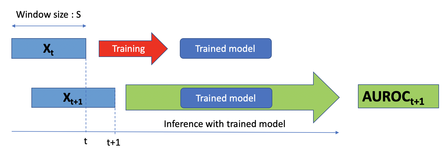
Figure 3: Process of generating $\mathbf{AUROC}_{t+1}$ from model trained at $t$

To asses the performance of the proposed measure, we will first look at correlations between $\mathbf{AUROC}_{t+1}$ (the next day GAE reconstruction) and $\text{RV}_{t+1}^{t+2}$ (the following day’s return volatility). This comparison is done by observing the variation of the time series, observing the KDE plots and the Spearman rank correlation of $\mathbf{AUROC}_{t+1}$ and $\text{RV}_{t+1}^{t+2}$. We chose the Spearman rank correlation as it is less vulnerable to outliers. High correlation between $\mathbf{AUROC}_{t+1}$ and $\text{RV}_{t+1}^{t+2}$ would indicate that changes in $\mathcal{G}_{t+1}$’s homogeneity compared with $\mathcal{G}_{t}$ are in sync with market instability.

As a second step, we then test the usefulness of $\mathbf{AUROC}_{t+1}$ for the forecasting of $\text{log}(\text{RV})$ at the following ${t+2}$ timestep ($\text{log}(\text{RV}_{t}^{t+2})$). We perform this forecasting with the HAR model for log-RV forecasting by Corsi, (2009). The HAR is a strong and industry recognised benchmark model for volatility forecasting Lim et al., (2020). It uses auto-regressive components of lower frequency past volatility to predict future volatility. Lower frequency volatility measurements are weekly and monthly volatility. Eq. 6 shows how the the HAR($\text{RV}_{t+2}$) operates, it learns a parameter $\beta_{n}$ for each previous volatility measure from the past time periods. We look at an 1-hour frequency of forecasting as it is a frequency of interest for industry practitioners Andersen et al., (2006); Onnela et al., (2004); Lim et al., (2020). We calculate the $R^{2}$ of this estimation for a linear regression, a XGBoost tree and an MLP as well as the $R^{2}$ of the estimation to which we add the $\mathbf{AUROC}_{t+1}$ as in Eq. 7. An increase in the $R^{2}$ of the forecasting model with the GAE-based measure added would suggest that the GAE encodes useful information for out-of-sample stability forecasting.

$$\text{log}(\text{RV}_{t+1}^{t+2})=HAR(\text{log}(\text{RV}_{t}^{t+1}))\sim\beta_{1}*\text{log}(\text{RV}_{t}^{t+1})+\beta_{2}*\text{log}(\text{RV}_{t-6}^{t+1})$$ (6)

$$\text{log}(\text{RV}_{t+1}^{t+2})\sim HAR(\text{log}(\text{RV}_{t}^{t+1}))+\beta_{3}*\mathbf{AUROC}_{t+1}$$ (7)

3 Results

3.1 Correlation between $\mathbf{AUROC}$ t+1 and volatility

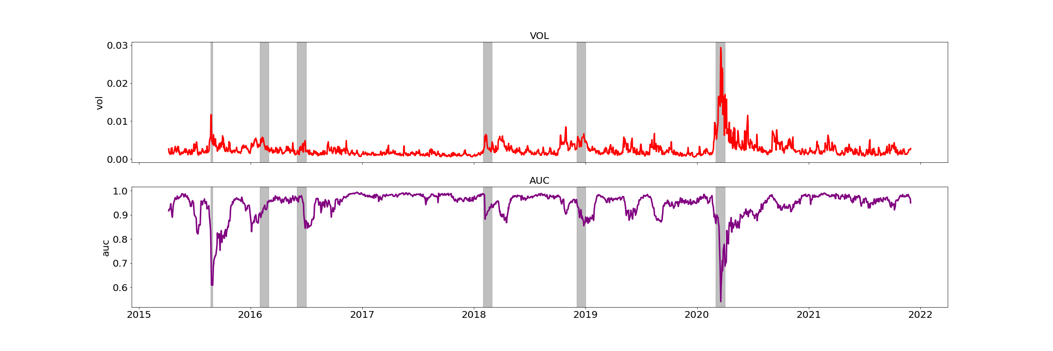
Figure 4: Time series of volatility vs $\mathbf{AUROC}_{t+1}$

When comparing the $\mathbf{AUROC}_{t+1}$ and market volatility, we remark that $\mathbf{AUROC}_{t+1}$ appears to co-move with volatility. $\mathbf{AUROC}_{t+1}$ is high in periods of relative market stability where volatility is lower and sharply fall during downturns and high-volatility markets where volatility is high. As GAE model performance is linked to the homogeneity of edge formation across a graph, the model shows lower performance during high-volatility periods. This suggests a more volatile market at $t+1$ correlates to heterogeneous edge formation in the market graph $\mathcal{G}_{t+1}$ which the GAE cannot learn as easily as those in more stable settings confirming the expectation laid out in the literature and our problem setting.

The six grey bands highlight periods of market instability, either due to so called ‘flash crashes’ as in late 2015 or those due to fundamental shifts in market stability such as the 2020 pandemic stock market collapse. These further allow us to remark that the $\mathbf{AUROC}_{t+1}$ seem to dip slightly before a volatility upswing, suggesting a useful application of these measures in forecasting, which is further investigated in the regression analysis results presented in Sec. 3.2.

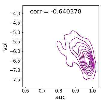
Figure 5: KDE of $\mathbf{AUROC}_{t+1}$ compared to volatility

The plots above show the kernel density distribution and Spearman rank correlation between log volatility and the $\mathbf{AUROC}_{t+1}$. The relationship between log volatility and the $\mathbf{AUROC}_{t+1}$ and the correlation in Fig. 5 displays an inverse relation between market stability and the GAE’s performance. This provides evidence in support of the expectation that the GAE produces a good measure for market instability as it encodes graph homogeneity, and drops in $\mathbf{AUROC}_{t+1}$ are correlated with increased volatility.

3.2 Next-day volatility forecasting

In this section, we move on from looking at how well the $\mathbf{AUROC}_{t+1}$ represents market instability. We shift our focus to looking at the usefulness of the $\mathbf{AUROC}_{t+1}$ to predict $\text{log}(\text{RV}_{t}^{t+1})$ the following day’s volatility.

Model	$R^{2}$ with $\mathbf{AUROC}_{t+1}$	$R^{2}$ without $\mathbf{AUROC}_{t+1}$	$p$-value of difference
Linear	$\mathbf{0.360^{*}}$	0.107	0.00
Tree	$\mathbf{0.357^{*}}$	0.310	0.043
MLP	$\mathbf{0.380^{*}}$	0.317	0.003

Note : * and bold font indicate $p$-value < 0.05.

Table 1: Results of log-RV forecasting at the 1-hour frequency

Table 1 presents the results of the log-RV forecasting task at time period $t+2$ defined in the methods by Eq. 6 and Eq. 7. The table compares the $R^{2}$ with and without the $\mathbf{AUROC}_{t+1}$. The $p$-value displayed on the rightmost column corresponds to a bootstrapped estimate of the significance of the difference between the MSE of the prediction in a one-sided statistical significance test checking whether the $R^{2}$ with the added $\mathbf{AUROC}_{t+1}$ is larger than the $R^{2}$ without. The $H_{0}$ null hypothesis is that the $R^{2}$ with $\mathbf{AUROC}_{t+1}$ is not significantly larger than the one without while the $H_{1}$ is that there is a statistically significant increase in $R^{2}$. The results show a statistically significant positive effect of the $\mathbf{AUROC}_{t+1}$ on the forecasting of hourly volatility. This result suggests that the $\mathbf{AUROC}_{t+1}$ of the GAE provides a signal that is useful in forecasting $t+2$ volatility.

4 Discussion and Conclusion

Our research investigated the link between the encoding ability of an unsupervised node-embedding model and market instability. The results above support our hypothesis that the the edge reconstruction accuracy of a GAE would serve as a good proxy to detect changes in the homogeneity of connectivity across a financial graph and thus serve as a good proxy for market volatility. The GAE’s encoding of market returns and connectivity at time step $t+1$ is correlated with market instability at the same time step as shown in Section 3.1 and useful in forecasting out-of-sample volatility as demonstrated in the regression analysis of Section 3.2. The novelty of our contribution lies in underlining the importance of looking at node features as well as the adjacency matrix when deriving stability indicators from financial networks. Moreover, we extended the literature on the use of graph neural networks in finance by successfully applying an unsupervised methodology to generating good-quality latent node representations which encode financial states.

Our approach is flexible and can be applied to other financial networks used in the literature to describe inter firm relations. Thus we aim to apply this approach to graphs constructed from news corpuses (Heiberger, , 2014) Wan et al., (2021), supply chains (Matsunaga et al., , 2019) or knowledge graphs (Hamilton, , 2020). These other types of graphs capture qualitatively different connections than correlations. That allows them to go beyond the statistical correlations we use to build the graph in this paper. This would allow us to learn instability-predictive features derived from other types of co-movement relations, and in turn refine the volatility forecasting. This same flexibility would allow us to study other edge formation structures which have seen intense interest from the standpoint of propagation of systemic risk such as inter-banking markets (Acemoglu et al., , 2015) or national stock markets indices. This methodology requires data on price movements of all considered companies for at least 20 days of price returns in order to generate a network. Thus one limitation of the proposed approach is that it cannot deal well with emergent companies with incomplete price data as those new firms price information could not be included in the network formation step.

We argue that by showing that homogeneity of graph connections is an important feature in market stability, this work also opens future areas for research. With that in mind, we discuss a set of extensions that address the limitations in our solution. The first proposed extension addresses a limitation of the current implementation related to static embeddings: we are currently learning node embeddings for a single static graph and testing the accuracy of the reconstruction on another static graph. In future work, we would like to explore a dynamic feature to the graph auto-encoder as in DynGAE (Mahdavi et al., , 2020). Another extension stems from the agreement between our unsupervised method using graph features and previously observed good performance of non-graph auto-encoder models in finance which attempted to reconstruct only returns Lim et al., (2020). We propose extending the current implementation to reconstruct both adjacency and returns such as in GALA architecture (Park et al., , 2019).

References

- Acemoglu et al., (2015) Acemoglu, D., Ozdaglar, A., and Tahbaz-Salehi, A. (2015). Systemic risk and stability in financial networks. American Economic Review, 105(2):564–608.
- Andersen et al., (2006) Andersen, T. G., Bollerslev, T., Christoffersen, P. F., and Diebold, F. X. (2006). Chapter 15 Volatility and Correlation Forecasting. Handbook of Economic Forecasting, 1:777–878.
- Artzner et al., (1999) Artzner, P., Delbaen, F., Eber, J. M., and Heath, D. (1999). Coherent measures of risk. Mathematical Finance, 9(3):203–228.
- Caccioli et al., (2018) Caccioli, F., Barucca, P., and Kobayashi, T. (2018). Network models of financial systemic risk: a review. Journal of Computational Social Science, 1(1):81–114.
- Campbell et al., (2002) Campbell, R., Koedijk, K., and Kofman, P. (2002). Increased Correlation in Bear Markets. Financial Analysts Journal, 58(1):87–94.
- Chami et al., (2022) Chami, I., Abu-El-Haija, S., Perozzi, B., Ré, C., and Murphy, K. (2022). Machine Learning on Graphs: A Model and Comprehensive Taxonomy. Journal of Machine Learning Research, 23(89):1–64.
- Chandra, (2003) Chandra, M. (2003). Multivariate GARCH modelling of volatility and comovements in Multivariate GARCH modelling of volatility and comovements in Asia Pacific markets Asia Pacific markets. Edith Cowan University.
- Corsi, (2009) Corsi, F. (2009). A simple approximate long-memory model of realized volatility. Journal of Financial Econometrics, 7(2):174–196.
- Das et al., (2019) Das, S. R., Kim, S., and N., O. D. (2019). Dynamic Systemic Risk:. Journal of Financial Data Science, pages 141–158.
- Estrada, (2010) Estrada, E. (2010). Quantifying network heterogeneity. Physical Review E - Statistical, Nonlinear, and Soft Matter Physics, 82(6):066102.
- Haldane, (2009) Haldane, A. (2009). Rethinking the Financial Network, Speech by Andrew Haldane, Executive Director, Financial Stability. Network, (April):1–41.
- Hamilton, (2020) Hamilton, W. L. (2020). Graph Representation Learning Hamilton. Synthesis Lectures on Artificial Intelligence and Machine Learning, 14(3):1–159.
- Heiberger, (2014) Heiberger, R. H. (2014). Stock network stability in times of crisis. Physica A: Statistical Mechanics and its Applications, 393:376–381.
- Kingma and Ba, (2015) Kingma, D. P. and Ba, J. L. (2015). Adam: A method for stochastic optimization. 3rd International Conference on Learning Representations, ICLR 2015 - Conference Track Proceedings.
- Kipf and Welling, (2016) Kipf, T. N. and Welling, M. (2016). Variational Graph Auto-Encoders.
- Kipf and Welling, (2017) Kipf, T. N. and Welling, M. (2017). Semi-supervised classification with graph convolutional networks. 5th International Conference on Learning Representations, ICLR 2017 - Conference Track Proceedings.
- Kukreti et al., (2020) Kukreti, V., Pharasi, H. K., Gupta, P., and Kumar, S. (2020). A Perspective on Correlation-Based Financial Networks and Entropy Measures. Frontiers in Physics, 8:323.
- Lim et al., (2020) Lim, B., Zohren, S., and Roberts, S. (2020). Detecting Changes in Asset Co-Movement Using the Autoencoder Reconstruction Ratio. SSRN Electronic Journal.
- Mahdavi et al., (2020) Mahdavi, S., Khoshraftar, S., and An, A. (2020). Dynamic joint variational graph autoencoders. Communications in Computer and Information Science, 1167 CCIS:385–401.
- Mantegna, (1999) Mantegna, R. N. (1999). Information and hierarchical structure in financial markets. Computer Physics Communications, 121:153–156.
- Matsunaga et al., (2019) Matsunaga, D., Suzumura, T., and Takahashi, T. (2019). Exploring Graph Neural Networks for Stock Market Predictions with Rolling Window Analysis. * Equal contribution. NeurIPS.
- Noureldin et al., (2012) Noureldin, D., Shephard, N., and Sheppard, K. (2012). Multivariate high-frequency-based volatility (HEAVY) models. Journal of Applied Econometrics, 27(6):907–933.
- Onnela et al., (2004) Onnela, J. P., Kaski, K., and Kertész, J. (2004). Clustering and information in correlation based financial networks. European Physical Journal B, 38(2):353–362.
- Park et al., (2019) Park, J., Lee, M., Chang, H. J., Lee, K., and Choi, J. Y. (2019). Symmetric graph convolutional autoencoder for unsupervised graph representation learning. Proceedings of the IEEE International Conference on Computer Vision, 2019-Octob:6518–6527.
- Preis et al., (2012) Preis, T., Kenett, D. Y., Stanley, H. E., Helbing, D., and Ben-Jacob, E. (2012). Quantifying the behavior of stock correlations under market stress. Scientific Reports, 2(1):1–5.
- Saha et al., (2022) Saha, S., Gao, J., and Gerlach, R. (2022). A survey of the application of graph-based approaches in stock market analysis and prediction. International Journal of Data Science and Analytics, 14(1):1–15.
- Samal et al., (2021) Samal, A., Pharasi, H. K., Ramaia, S. J., Kannan, H., Saucan, E., Jost, J., and Chakraborti, A. (2021). Network geometry and market instability. Royal Society Open Science, 8(2).
- Sandhu et al., (2016) Sandhu, R. S., Georgiou, T. T., and Tannenbaum, A. R. (2016). Ricci curvature: An economic indicator for market fragility and systemic risk. Science Advances, 2(5).
- Serur and Avellaneda, (2021) Serur, J. A. and Avellaneda, M. (2021). Hierarchical PCA and Modeling Asset Correlations. SSRN Electronic Journal.
- Tumminello et al., (2010) Tumminello, M., Lillo, F., and Mantegna, R. N. (2010). Correlation, hierarchies, and networks in financial markets. Journal of Economic Behavior and Organization, 75(1):40–58.
- Wan et al., (2021) Wan, X., Yang, J., Marinov, S., Calliess, J. P., Zohren, S., and Dong, X. (2021). Sentiment correlation in financial news networks and associated market movements. Scientific Reports, 11(1):1–12.
- Wang et al., (2022) Wang, J., Zhang, S., Xiao, Y., and Song, R. (2022). A Review on Graph Neural Network Methods in Financial Applications. Journal of Data Science, pages 111–134.
- Xue et al., (2022) Xue, J., Jiang, N., Liang, S., Pang, Q., Yabe, T., Ukkusuri, S. V., and Ma, J. (2022). Quantifying the spatial homogeneity of urban road networks via graph neural networks. Nature Machine Intelligence, 4(3):246–257.
- Zhao et al., (2016) Zhao, L., Li, W., and Cai, X. (2016). Structure and dynamics of stock market in times of crisis. Physics Letters A, 380(5-6):654–666.