PDE-LEARN: Using Deep Learning to Discover Partial Differential Equations from Noisy, Limited Data
Abstract
In this paper, we introduce PDE-LEARN, a novel deep learning algorithm that can identify governing partial differential equations (PDEs) directly from noisy, limited measurements of a physical system of interest. PDE-LEARN uses a Rational Neural Network, , to approximate the system response function and a sparse, trainable vector, , to characterize the hidden PDE that the system response function satisfies. Our approach couples the training of and using a loss function that (1) makes approximate the system response function, (2) encapsulates the fact that satisfies a hidden PDE that characterizes, and (3) promotes sparsity in using ideas from iteratively reweighted least-squares. Further, PDE-LEARN can simultaneously learn from several data sets, allowing it to incorporate results from multiple experiments. This approach yields a robust algorithm to discover PDEs directly from realistic scientific data. We demonstrate the efficacy of PDE-LEARN by identifying several PDEs from noisy and limited measurements.
Keywords: Deep Learning, Sparse Regression, Partial Differential Equation Discovery, Physics Informed Machine Learning
1 Introduction
Scientific progress is contingent upon finding predictive models for the natural world. Historically, scientists have discovered new laws by studying physical systems to distill the first principles that govern those systems. This first-principles approach has yielded predictive models in many fields, including fluid mechanics, population dynamics, quantum mechanics, and general relativity. Unfortunately, despite years of concerted effort, many systems currently lack predictive models, particularly those in the biological sciences [1], [3].
These roadblocks call for a new approach to identifying governing equations. At its core, discovering new scientific laws relies on identifying simple governing equations from complex data sets. Pattern recognition is, notably, one of the core goals of machine learning. Advances in machine learning, specifically deep learning, offer an intriguing alternative approach to discovering scientific laws. The burgeoning field of physics-informed machine learning seeks to use machine learning for scientific and engineering applications by designing models whose architecture incorporates knowledge of the physical system. PDE discovery, a sub-field of physics-informed machine learning, seeks to use machine learning models to identify partial differential equations (PDEs) from data. PDE discovery may be able to discover predictive models for physical systems that have proven difficult to model.
Crucially, any approach that aims to discover scientific laws must be able to work with scientific data. Scientific data sets are often limited (sometimes only a few hundred data points) and may contain substantial noise. Therefore, PDE discovery algorithms must be able to work with limited, noisy data. Further, scientists often perform multiple experiments on the same system. As such, PDE discovery algorithms should be able to incorporate information from multiple data sets. This paper presents a novel PDE discovery algorithm that meets these challenges.
Contributions: In this paper, we develop a novel PDE discovery algorithm, PDE-LEARN, that can learn a general class of PDEs directly from data. In particular, PDE-LEARN can identify both linear and nonlinear PDEs with several spatial variables. Significantly, PDE-LEARN is also robust to noise and limited data. Further, PDE-LEARN can pool information from multiple experiments, by learning from multiple data sets simultaneously. We confirm PDE-LEARN’s efficacy through a set of numerical experiments. These experiments demonstrate that PDE-LEARN can discover a variety of linear and nonlinear PDEs, even when its training set is limited and noisy.
Outline: The rest of this paper is organized as follows: First, in section 2, we state our assumptions on the data and the form of the hidden PDE. Next, in section 3, we survey related work on PDE discovery, focusing on methods that encode the hidden PDE into their loss functions. In section 4, we give a comprehensive description of the PDE-LEARN algorithm. In section 5, we demonstrate the efficacy of PDE-LEARN by discovering a variety of PDEs from limited, noisy data sets. Section 6 discusses our rationale behind the PDE-LEARN algorithm, practical considerations, limitations, and potential future research directions. Finally, we provide concluding remarks in section 7.
2 Problem Statement
Our algorithm uses noisy measurements of one or more system response functions to identify a hidden PDE that those system response functions satisfy. This section mainly serves to make the preceding statement more precise. First, we introduce the notation we use throughout this paper. We then define what we mean by system response functions and state our assumptions about the hidden PDE they satisfy. We then specify our assumptions about our noisy measurements of the system response function. Finally, we conclude this section by formally stating the problem that our approach seeks to solve.
Problem domain: Let and be a collection of open, connected sets. We refer to as the th spatial problem domain. We assume that for each , a physical process evolves on the domain during the time interval , for some . Thus, there exists a system response function that describes the state of the th physical process at each position and time. In particular, denotes the system state at time and position . We refer to the Cartesian product as the th problem domain. If , we drop the subscript notation and refer to as the problem domain.
Roughly speaking, we assume that each system response function corresponds to an experiment. Thus, by allowing multiple system response functions, we can deal with the case when the user has has data from several experiments. It is also possible, and perfectly admissible, to have just one problem domain and response function.
Derivative Notation: In this paper, denotes the th partial derivative of any sufficiently smooth function with respect to the variable . Thus, for example,
For brevity, we abbreviate as . Throughout this paper, it will be helpful to have a concise notation for all partial derivative operators below a certain order. With that in mind, let
denote an enumeration of the partial derivatives of of order (with the convention that the identity map is a th-order partial derivative). Note that includes mixed partials if is a function of multiple variables.
As an example, let’s consider the case when and . Thus, we are interested in all partial derivatives of order of a function of three variables, , , and . In this case, , and one possible enumeration is
As this example demonstrates, does not necessarily represent a fifth-order partial derivative of . Rather, denotes the fifth term in our specific enumeration of the partial derivatives of .
Hidden PDE: We assume there exists a hidden PDE of order such that satisfies the hidden PDE on . We further assume this PDE takes the following form:
| (1) |
Critically, we assume that equation 1 holds with the same coefficients for each . In this expression, we refer to the functions as the library terms. We refer to as the left-hand side term or LHS term for short. We also refer to as the right-hand side terms or RHS terms for short. Each library term is a function of and its partial derivatives (both in space and time) of order .
At a high level, the algorithm we propose attempts to learn the coefficients using noisy, limited measurements of the system response functions and an assumed set of library terms. Before we can state our algorithm precisely, we need to make a few assumptions about the library and the system response data.
Monomial Library Terms: Many physical systems are governed by equation 1 for a particular and set of coefficients. In many cases of practical interest (e.g. solid and fluid mechanics, thermodynamics, and quantum mechanics), the governing PDE consists of terms that are monomials of and its partial derivatives. That is, the terms are of the form
| (2) |
For some . We call library functions of this form monomial library functions. In this paper, we consider libraries consisting of monomial library terms. In principle, however, our proposed algorithm can work with any library.
Data Points: Let and let be a collection of data points in the th problem domain. We assume that we have noisy measurements of at these data points, which we denote by
We refer to the collection of these measurements as the th noisy data set. Further, we refer to the corresponding set as the th noise-free data set. Critically, we only assume knowledge of the noisy data set. In general, since the measurements are noisy,
We assume, however, that for each ,
for some . We refer to this difference as the noise at the data point . We assume that the noises at different data points are independent and identically distributed. We define the noise level of a data set as the ratio of to the standard deviation of the noise-free data set. Finally, if , we write for .
Goals: Our goal is to use the noisy data sets, , and the library, , to learn the coefficients in equation 1. To do this, we learn an approximation to each that satisfies equation 1 for some set of coefficients. To maximize the applicability of our approach, we make as few assumptions as possible about the hidden PDE. In particular, we generally use a large library. The goal here is to select a library that is broad enough to include the terms that are present (have non-zero coefficients) in the hidden PDE without requiring the user to identify those terms beforehand. This approach means our library includes many extraneous terms; i.e., most of the coefficients should be zero. Therefore, we tacitly assume the right-hand side of equation 1 is sparse.
For reference, table 1 lists the notation we introduced in this section.
| Notation | Meaning |
|---|---|
| The number of spatial dimensions in the spatial problem domain. | |
| The number of system response functions. | |
| The th spatial domain111For a given problem, all spatial domains come from the SAME Euclidean subspace. That is, for each .: an open, connected subset of . | |
| The time interval over which evolves on . | |
| The th system response function. If , we denote . | |
| The number of distinct partial derivatives of of order . | |
| An enumeration of the partial derivatives of order (including the identity map). | |
| the th derivative of some function with respect to the variable . | |
| abbreviated notation for . | |
| Number of data points in the th noisy-data set. If , we write . | |
| The data points for the th system response function. | |
| A noisy measurement of at . | |
| The number of library functions. See equation 1 | |
| The left-hand side term. See equation 1. | |
| The right-hand side terms. See equation 1. | |
| The coefficients of the RHS terms terms in equation 1. | |
| Noise level | The ratio of the standard deviation of the noise to that of the noise-free data set. |
3 Related Work
In this section, we discuss relevant previous work on PDE discovery to contextualize our contributions. PDE discovery began in the late 2000s with two papers, [9] and [29]. While neither paper is directly concerned with identifying PDEs (the former focuses on discovering dynamical systems, while the latter focuses on identifying invariant and conservation laws), they set the stage for using machine learning to discover scientific laws from data. Both approaches use genetic algorithms to learn relationships (hidden dynamical system in the former and conservation laws in the latter) that the system response function satisfies.
A significant advance came a few years after [29] when Rudy et al. introduced PDE-FIND [27]. Developed as a modification of the Sparse Identification of Nonlinear DYnamics (SINDY) algorithm [13], PDE-FIND represents one of the earliest and most important breakthroughs in identifying PDEs directly from data. PDE-FIND uses similar assumptions to the ones listed in section 2 but additionally assumes that (a single experiment), , and the RHS terms depend only on the lone system response function, , and its spatial partial derivatives. Critically, PDE-FIND also assumes the data points occur on a regular grid. This additional constraint allows PDE-FIND to use numerical differentiation techniques to approximate the partial derivatives of . Using these approximations, PDE-FIND can evaluate the library terms at the data points, which engenders a linear system for the coefficients . PDE-FIND then finds a sparse, approximate solution to this system using an algorithm called Sequentially Thresholded Least Squares, or ST-Ridge for short. PDE-FIND can successfully identify a wide range of PDEs directly from data. With that said, PDE-FIND does have some fundamental limitations. In particular, since numerical differentiation tends to amplify noise, PDE-FIND’s performance decreases considerably in the presence of moderate noise levels. Further, requiring the data to occur on a regular grid is a cumbersome limitation for scientific applications, where data can be difficult and expensive to acquire.
In addition to PDE-FIND, two other notable examples of early PDE discovery algorithms are [28] and [8]. The former is similar to PDE-FIND but uses spectral methods to approximate the derivatives. This change enables their approach to identify a variety of PDEs, even in the presence of significant noise. Like PDE-FIND, however, [28] does require that the data points occur on a regular grid. The latter trains a neural network, , to match a noisy data set (thereby learning an approximation to the system response function) and then uses sparse regression to identify the coefficients . Using a network to interpolate the data allows the data points to be dispersed anywhere in the problem domain.
Another significant contribution to PDE discovery came a few years later with DeepMoD [11]. DeepMoD learns an approximation, , to the coefficients , while simultaneously training a neural network, , to match a noisy data set. Thus, their approach learns the hidden PDE and the system response function at the same time. Further, like [8], the data points for DeepMoD can be arbitrarily distributed throughout the problem domain. DeepMoD uses Automatic Differentiation [7] to calculate the partial derivatives of the neural network at randomly selected collocation points in the problem domain. DeepMoD can then use these partial derivatives to evaluate the library terms at the collocation points. To train and , DeepMoD uses a three-part loss function. The first part measures how well matches the data set, the second measures how well satisfies the hidden PDE 1 with the components of in place of , and the third is the norm of (this promotes sparsity in ). The second and third parts of the loss function embed the LASSO loss function within DeepMoD’s loss function. These parts encourage to learn the function that roughly matches the data but also satisfies a PDE of the form of equation 1. This approach embeds the fact that the system response function satisfies a PDE characterized by into the loss function. This loss function produces a robust algorithm that can identify PDEs, even from noisy and limited data. DeepMoD served as the original inspiration for PDE-LEARN. Finally, it is worth noting that [15] proposed an approach similar to DeepMoD but uses an innovative training scheme that achieves impressive results on several PDEs.
More recently, the authors of this paper proposed another algorithm, PDE-READ [31]. PDE-READ uses two neural networks: The first, , learns the system response function, and the second, , learns an abstract representation of the right-hand side of equation 1. That approach is based on Raissi’s deep hidden physics models algorithm [26]. Like DeepMoD, PDE-READ learns an approximation of the system response function while simultaneously identifying the hidden PDE. Significantly, PDE-READ utilizes Rational Neural Networks [12], a type of fully connected neural network whose activation functions are trainable rational functions. After training both networks, PDE-READ uses a modified version of the Recursive Feature Elimination algorithm [19] to extract from . This approach proves impressively robust, as PDE-READ can identify a variety of PDEs even from limited measurements with very high noise levels.
The methods discussed above mostly use a standard fully connected neural network to approximate the system response function and identify the hidden PDE. The PDE-discovery community has, however, proposed many other approaches. [18] and [24] learn the hidden PDE via a weak-formulation approach. Using weak forms places additional restrictions on the form of the hidden PDE but engenders an algorithm that is remarkably robust to noise. Further, [4] uses a Gaussian process to approximate the system response function and a genetic algorithm to identify the hidden PDE. Finally, [10] uses Bayesian Neural networks to learn the system response function and identify the hidden PDE.
In this paper, we introduce a new PDE discovery algorithm, PDE-LEARN. PDE-LEARN can learn a broad class of PDEs directly from noisy and limited data. Like PDE-READ, PDE-LEARN utilizes Rational Neural Networks [12] to learn an approximation of the system response functions. Further, like DeepMoD, PDE-LEARN uses a sparse, trainable vector, , to learn an approximation to the coefficients . What sets PDE-LEARN apart, however, is its three-part loss function that incorporates aspects of the iteratively reweighted least-squares algorithm [14] to help promote sparsity in . Equally important, PDE-LEARN uses an adaptive procedure to place additional collocation points in regions where the collocation loss is the greatest. This process helps accelerate convergence and yields an algorithm that is highly effective in the low-data, high-noise data limit.
4 Methodology
In this section, we describe our algorithm - PDE discovery via Error Approximation and Rational Neural networks - or PDE-LEARN for short. PDE-LEARN does the following: First, it uses noisy data sets, , to learn an approximation to each system response function, . Second, it uses the fact that the system response functions satisfy a PDE of the form of equation 1 to learn the coefficients . Significantly, PDE-LEARN can learn any PDE of the form of equation 1 and can operate with multiple spatial variables.
PDE-LEARN uses a Rational Neural Network [12], , to approximate the th system response function, . It approximates the coefficients in equation 1 using a trainable vector, . During training, PDE-LEARN learns and each by minimizing the loss function
| (3) |
Here, , , and are user-selected scalar hyperparameters. Further,
| (4) | |||
| (5) | |||
| (6) |
In equation 6, PDE-LEARN updates the constants at the start of each epoch such that the loss approximates the norm of . We discuss this in detail in section 4.2. In equation 5, is the PDE-Residual, defined by
| (7) |
where is an abbreviation for . PDE-LEARN uses automatic differentiation [7] to calculate the partial derivatives of and subsequently evaluate the library functions. The points are the collocation points. We discuss these in detail below in section 4.1.
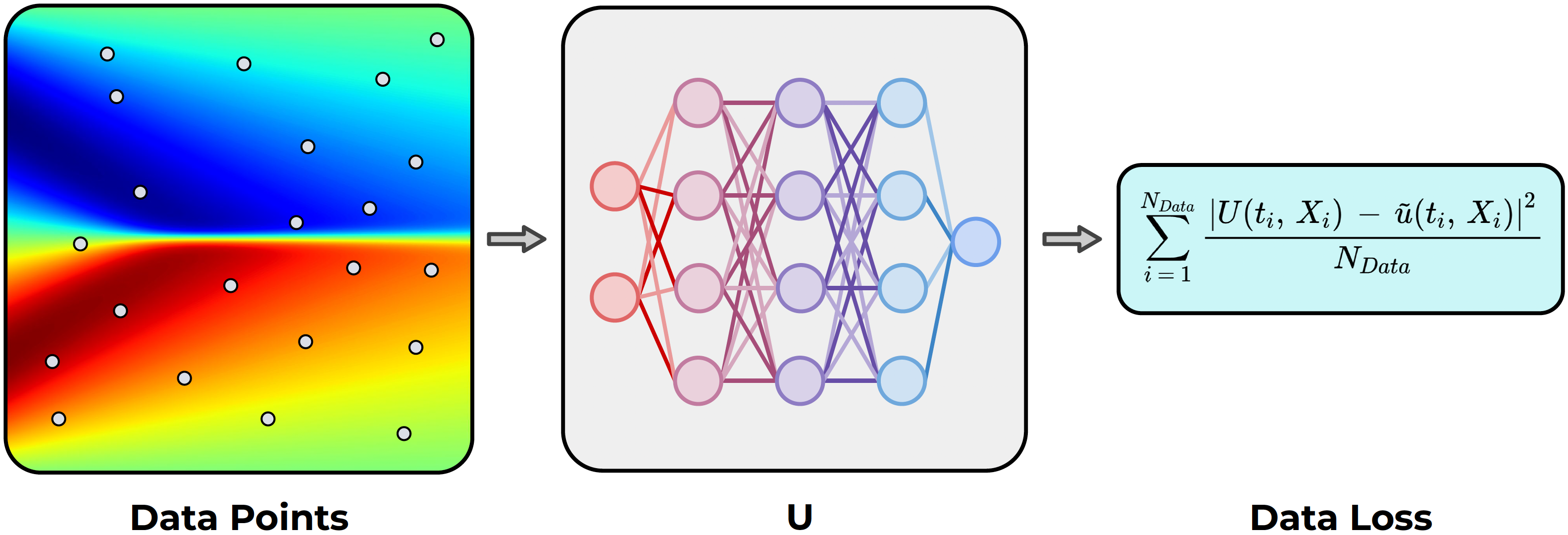
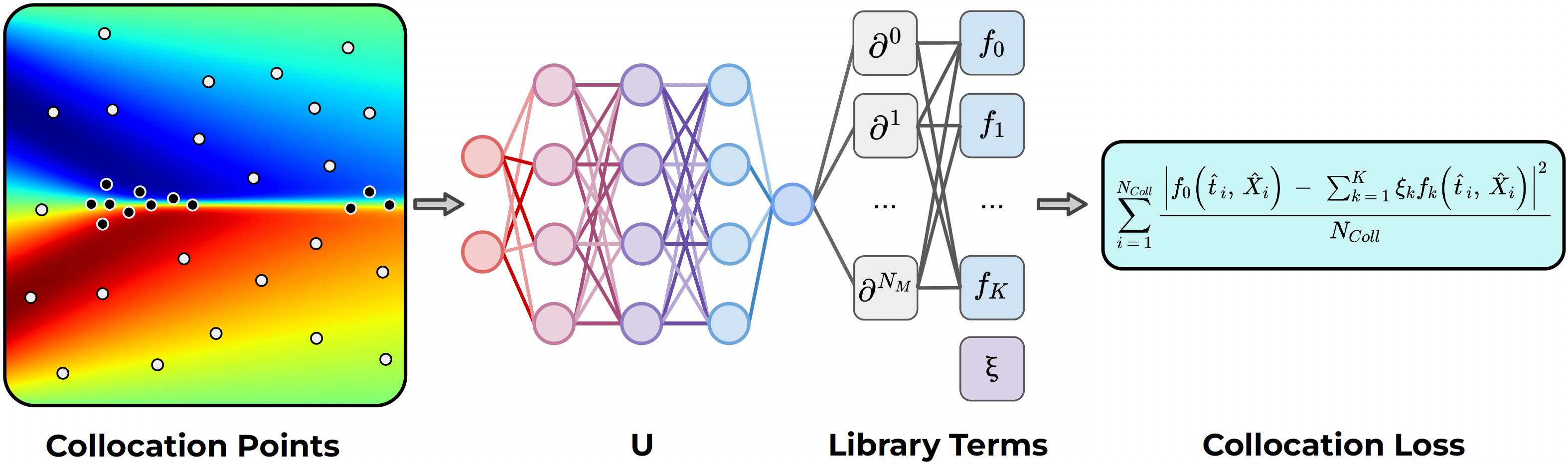
We refer to , , and as the Data, Collocation, and Lp losses, respectively. Figures 1 and 2 depict how PDE-LEARN evaluates the Data and Collocation Losses, respectively.
The Data Loss forces to satisfy the noisy data, at the data points. It is the mean square error between ’s predictions and the noisy data set. The collocation loss forces to satisfy the PDE encoded in
at the collocation points . It is what couples the training of and . Finally, encodes our assumption that most of the coefficients in equation 1 are zero by promoting sparsity in . It is a weighted sum of the squares of components of . PDE-LEARN accomplishes this by re-selecting the weights, , at the start of each epoch. We discuss this in detail in section 4.2.
To use PDE-LEARN, one must provide a noisy data set, select an architecture for , and select an appropriate collection of library terms. Here, appropriate means that the right-hand side of the hidden PDE can be expressed as a sparse linear combination of the library terms. Once PDE-LEARN has finished training, it reports identified PDE.
4.1 Collocation Loss
In equation 7, is the PDE residual of at the collocation point . PDE-LEARN uses two types of collocation points: random collocation points and targeted collocation points. Each problem domain has collocation points (both random and targeted). For each problem domain, PDE-LEARN selects the random collocation points by repeatedly sampling from a uniform distribution over the problem domain,
The number of random collocation points in each problem domain, , is a hyperparameter. PDE-LEARN re-samples the random collocation points for each problem domain at the start of each epoch. The targeted collocation points are the random collocation points from previous epochs at which the PDE residual is unusually large. At the start of training, we initialize the targeted collocation points to be the empty set. During subsequent epochs, PDE-LEARN uses the following procedure for each system response function:
-
1.
During each epoch PDE-LEARN records the absolute value of the PDE residual at each collocation point (both random and targeted) for the th system response function. PDE-LEARN records this set of non-negative values.
-
2.
PDE-LEARN then computes the mean and standard deviation of this set.
-
3.
PDE-LEARN then determines which collocation points have an absolute PDE-Residual that is more than three standard deviations larger than the mean. These points are the targeted collocation points for the next epoch.
This procedure accelerates training by adaptively focusing the training of and on regions of the problem domain where the PDE residual is large. If the PDE residual is large in a particular region of the th problem domain, any collocation points in that region will become targeted collocation points. Because the random collocation points are re-sampled, new collocation points will appear in the problematic region at the start of each epoch. Thus, targeted collocation points will accumulate in that region. Eventually, the PDE residual in that region will dominate the collocation loss. This forces and to adjust until the PDE residual in the problematic region shrinks.
Though PDE-LEARN can work with an arbitrary collection of library functions, we only consider monomial library functions in this paper. To evaluate these functions efficiently, PDE-LEARN records every partial derivative operator that is present in at least one library function (equivalently, ). At the start of each epoch, PDE-LEARN evaluates these partial derivatives of each at each collocation point. We implemented this process to be as efficient as possible. In particular, it starts by computing the lowest-order partial derivatives of . For subsequent partial derivatives, PDE-LEARN uses the following rule: if we can express a partial derivative of as a partial derivative operator applied to another partial derivative of that we have already computed, then compute the new partial derivative from the old one. This approach allows us to compute all the necessary partial derivatives of without any redundant computations. After computing the partial derivatives of , PDE-LEARN uses them to evaluate the library terms at the collocation points. It then evaluates the PDE-Residual, equation 7, at each collocation point. Finally, from the PDE residuals, PDE-LEARN can compute the collocation loss, equation 5. Figure 2 depicts the process that PDE-LEARN uses to calculate the Collocation Loss.
4.2 Lp Loss
The collocation and losses embed the iteratively reweighted least-squares [14] loss function into ours. At the start of each epoch, PDE-LEARN updates the weights in equation 6 using the following rule:
| (8) |
Here, is a small constant to prevent division by zero, and is a hyperparameter. Crucially, the value that appears in this equation is the th component of at the start of the epoch; thus is treated as a constant during backpropagation. Notably, if is sufficiently large, then
and so,
Critically, PDE-LEARN evaluates each at the start of every epoch and treats them as constants during that epoch. This subtle detail allows to closely approximate while remaining a smooth, convex function of ’s components. We discuss this in section 6.3.
4.3 Training
PDE-LEARN identifies the hidden PDE using a three-step training process. We use the Adam [20] optimizer to minimize 3 in all three steps.
We call the first step the burn-in step. PDE-LEARN first initializes and the ’s. It initializes to a vector of zeros. It initializes the weights matrices and bias vectors in using the initialization procedure in [17]. Finally, it initializes the rational activation functions using the procedure in [12]. PDE-LEARN then sets to zero and begins training. During this step, learns an approximation to . Since , almost all components of become non-zero; we do not attempt to identify the PDE during this step.
At the end of the burn-in step, PDE-LEARN prunes by eliminating all RHS terms whose corresponding component of is smaller than a threshold. Throughout this paper, we select the threshold to be slightly larger than , where is machine epsilon for single-precision floating numbers. We discuss the implications of pruning in section 6.2.
In the second step, which we call the sparsification step, we set to a small, non-zero value and then resume training. During this step, becomes sparse, only retaining the components of that correspond to RHS terms that are present in the hidden PDE. After training, we repeat the pruning process (which usually eliminates the bulk of the extraneous RHS terms). By the end of this step, PDE-LEARN identifies which RHS terms have non-zero coefficients. However, since the loss encourages each coefficient to go to zero, the magnitudes of the retained coefficients are usually too small at this point.
In the third step, which we call the fine-tuning step, we set to zero once again and resume training. This step retains only the RHS terms that survived the sparsification step. By removing the loss, the components of are no longer under pressure to be as close to as possible, which allows them to converge to the values in the hidden PDE. PDE-LEARN trains until the loss stops increasing. PDE-LEARN then reports the identified PDE encoded in .
For brevity, we will let , , and denote the number of burn-in, sparsification, and fine-tuning epochs, respectively
Table 2 lists the notation we introduced in this section.
| Notation | Meaning |
|---|---|
| Neural Network to approximate . | |
| A trainable vector in whose components approximate . See equation 1. | |
| A hyperparameter representing the “p” in “”. See equation 6. | |
| The data loss. It measures the mean square error between and the noisy measurements of at the th data points. See equation 4 | |
| The collocation loss. It measures how well satisfies the hidden PDE encoded in at the collocation points. See equation 5. | |
| The loss. It represents the quasi-norm of raised to the th power. See equation 6. | |
| The PDE-residual. See equation 7. | |
| An abbreviation of . | |
| Hyperparameters that specify the weight of , , and , respectively. See equation 3. | |
| The number of collocation points for . See equation 5. | |
| A hyperparameter specifying the number of random collocation points. We use the same value for each system response function. See sub-section 4.1. | |
| The th set of collocation points. See equation 5. | |
| The number of burn-in epochs. | |
| The number of sparsification epochs. | |
| The number of fine-tuning epochs. |
5 Experiments
We implemented PDE-LEARN as an open-source Python library. Our implementation is publicly available at https://github.com/punkduckable/PDE-LEARN, along with auxiliary MATLAB scripts to generate our data sets.
As stated in section 4, each is a rational neural network [12]. Thus, ’s activation functions are trainable rational functions (rd order polynomial in the numerator, second-order polynomial in the denominator). In other words, the coefficients that define the numerator and denominator polynomials are trainable parameters that the network learns along with its weight matrices and bias vectors. Each hidden layer gets its own activation function, which we apply to each hidden unit in that layer.
In this section, we test PDE-LEARN on several PDEs, both linear and non-linear. All of the data we use in these experiments come from numerical simulations. The data sets from these simulations represent our noise-free data sets. To create noisy, limited data sets with points and a noise level , we use the following procedure:
-
1.
Calculate the standard deviation, , the samples of the system response function in the noise-free data set.
-
2.
Select a subset of size from the noise-free data set by sampling points from the noise-free data set without replacement. The resulting subset is the limited data set.
-
3.
Independently sample a Gaussian Distribution with mean and standard deviation once for each point in the limited data set. Add the th value to the th point in the limited data set. The resulting set is our noisy, limited data set.
As discussed in section 4.3, we use a three-step training process to train and . In our experiments, we stop the burn-in step when loss stops decreasing, which often takes between and epochs. For the sparsification step, we select a small value (usually ) and train until the loss stabilizes for a few hundred epochs (usually to epochs after burn-in). Finally, for the fine-tuning step, we stop training once the loss stops increasing or once an equation-specific222For every equation except the Allen-Cahn equation, we use an upper limit of fine-tuning epochs. In these experiments, the loss generally stops changing by that time. For the Allen-Cahn equation, however, the loss takes much longer to stabilize, so we use an upper limit of fine-tuning epochs. of fine-tuning epochs are complete.
In our experiments, all three steps use the Adam optimizer [20] with a learning rate of . Though we do not use it in our experiments, our implementation supports the LBFGS optimizer [23].
In every experiment in this section, we set and (see section 4.3). We did not attempt to optimize these values and do not claim they are optimal. However, we found them to be sufficient in our experiments.
5.1 Burgers’ equation
Burgers’ equation is a non-linear second-order non-linear PDE. It was first studied in [6] but arises in many contexts, including Fluid Mechanics, Nonlinear Acoustics, Gas Dynamics, and Traffic Flow [5]. Burgers’ equation has the form
| (9) |
where velocity, , is a function of and . Here, is the diffusion coefficient. Significantly, solutions to Burgers’ equation can develop shocks (discontinuities).
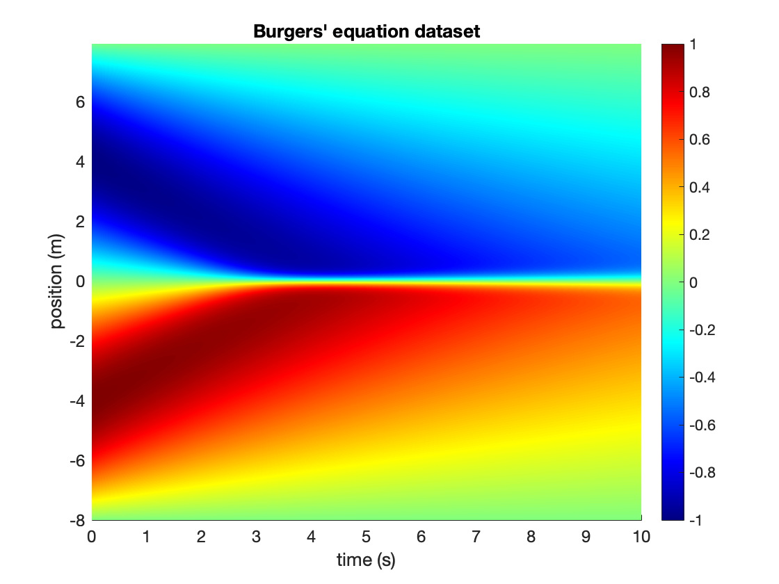
We test PDE-LEARN on a Burgers’ equation with on the domain . Thus, for these experiments, . For this data set,
To make the noise-free data set, we partition the problem domain using a spatiotemporal grid with grid lines along the -axis and along the -axis. Thus, each grid square has a length of along the -axis and a length of along the -axis. Our script Burgers_Sine.m (in the MATLAB sub-directory of our repository) uses Chebfun’s [16] spin class to find a numerical solution to Burgers’ equation on this grid. Figure 3 depicts the noise-free data set.
Using the procedure outlined at the beginning of section 5, we generate several noisy, limited data sets from the noise-free data set. We test PDE-LEARN on each data set. In each experiment, contains five layers with neurons per layer. For these experiments, the left-hand side term is
Likewise, the right-hand side terms are
Thus, our library includes terms with up to third-order spatial derivatives and fourth-order multiplicative products. For these experiments, we use burn-in epochs (), sparsification epochs () with , and a variable number of fine-tuning epochs (). Table 3 reports the results of our experiments with Burgers’ equation.
| Noise | Identified PDE | ||||
|---|---|---|---|---|---|
| 1 | |||||
| 1 | |||||
-
1
For these experiment, we use during the sparsification step. If we set , PDE-LEARN identifies in the , noise experiment and in the , noise experiment.
Thus, PDE-LEARN successfully learns Burgers’ equation in all but one of the experiments. PDE-LEARN can identify Burgers’ equation from data points even when we corrupt the data set with noise. If the noise level decreases to just , PDE-LEARN can reliably identify Burgers’ equation with as few as data points. Increasing the noise tends to increase the relative error between the identified and the corresponding coefficients in the hidden PDE. With that said, in the noise and data point experiment, the relative error of identified coefficients is .
Notably, PDE-LEARN fails to identify Burgers’ equation in one of the experiments. Even in this experiment, however, PDE-LEARN correctly identifies the RHS term . This result suggests that even when PDE-LEARN fails, it may still extract useful information about the hidden PDE. Interestingly, when , PDE-LEARN successfully identifies Burgers’ equation when the noise level is but not when it is . This result suggests that the number of measurements, not the noise level, is the main limiting factor in the low-data limit.
5.2 KdV Equation
Next, we consider The Korteweg–De Vries (KdV) equation, a non-linear third-order equation. [21] derived the KdV equation to describe the evolution of one-dimensional, shallow-water waves. With appropriate scaling, the KdV equation is
| (10) |
where wave height, , is a function of and .
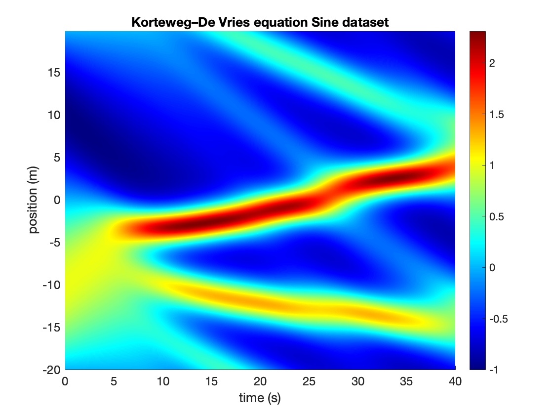
We test PDE-LEARN on the KdV equation on the domain . For this equation, we consider two initial conditions:
and
We partition the problem domain into a spatiotemporal grid with grid lines along the -axis and along the -axis. We use Chebfun’s [16] spin class to solve the KdV equation with each initial condition on this grid. We refer to the resulting solutions as our noise-free KdV- and KdV-- data sets, respectively. The scripts KdV_Sine.m and KdV_Exp_Cos.m in the MATLAB sub-directory of our repository generate these data sets. Figures 4 and 5 depict the data sets.
In all of our experiments with the KdV equation, contains four layers with neurons per layer333We tried using the same architecture as in the Burgers’ experiments. However, we found that architecture was too simple to learn the intricacies of the KdV data sets.. Further, we use the same left and right-hand side terms as in the Burgers’ experiments.
5.2.1 KdV sin data set
We test PDE-LEARN on several noisy, limited data sets built using the two noise-free data sets. We test PDE-LEARN on each data set. For these experiments, burn-in takes between and epochs using the Adam optimizer (stopping once the data loss stops decreasing). For the sparsification step, we use and train for between and epochs (stopping once the loss remains roughly constant for at least epochs). Table 4 reports our experimental results with the KdV- data set.
| Noise | Identified PDE | ||||
|---|---|---|---|---|---|
These results show that PDE-LEARN can identify the KdV equation from limited measurements, even at high noise levels. As in the Burgers experiments, the identified coefficients tend to be more accurate in lower noise experiments. Interestingly, PDE-LEARN can identify the KdV equation from the data set with as few as data points and % noise.
With that said, PDE-LEARN does have its limits. In particular, PDE-LEARN fails to identify the KdV equation in a few experiments. The identified PDE is too sparse in the data points, % noise, and data points, % noise experiments. In both cases, however, PDE-LEARN correctly identifies the RHS-term . By contrast, the identified PDE contains extra terms in the data points, % noise, and data points, noise experiments. In these experiments, the identified PDE contains both terms of the KdV equation (in addition to some extra ones). These results strengthen our assertion that PDE-LEARN identifies useful information even when it fails. If the identified PDE is too sparse, the terms in the identified PDE are likely to be present in the hidden PDE. Likewise, if the identified is not sparse enough, the terms of the hidden PDE are likely to be in the identified PDE.
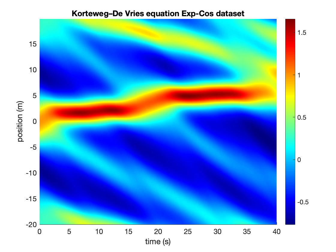
5.2.2 KdV exp-cos data set
Next, we test PDE-LEARN on the KdV - data set. For these experiments, burn-in takes epochs. For the sparsification step, we set and train for epochs. Table 5 reports our experimental results with the KdV - data set.
| Noise | Identified PDE | ||||
|---|---|---|---|---|---|
| 1 | |||||
-
1
We stop the burn in step after just epochs for the data point, % noise experiment. This is because the solution network began over-fitting the data set.
Once again, PDE-LEARN correctly identified the KdV equation under several noise levels across several data set sizes. Significantly, it identifies the KdV equation from just data points with % noise. Further, as in with the data set, PDE-LEARN successfully identified the KdV equation from data points and % noise.
As with the data set, however, PDE-LEARN does have limits. It fails to identify Burger’s equation in the data points, % noise experiment, and the data points, % noise experiments. In the former, the identified PDE is too sparse, though the lone term in the identified PDE, , is present in the KdV equation. The latter is more concerning, as the term is in the identified PDE, while one of the terms of the KdV equation, , is not. With that said, even in this case, PDE-LEARN did correctly identify one of the terms in the KdV equation, . These result suggest that PDE-LEARN fails only under extreme conditions and can still yield useful information when it does fail.
5.2.3 Combined data sets
Finally, to demonstrate that PDE-LEARN can learn from multiple data sets simultaneously (assuming the corresponding system response functions satisfy a common PDE), we test with the and - data sets simultaneously. For these experiments, burn-in takes epochs using the Adam optimizer (stopping once the data loss stops decreasing). For the sparsification step, we use and train for between epochs. For the combined data sets, we only consider conditions that cause PDE-LEARN trouble when learning from a single data set. Table 6 reports our experimental results for the combined KdV data set experiments.
| Noise | Identified PDE | ||||
|---|---|---|---|---|---|
-
1
Due to over-fitting, we stop burn in after epochs in the data point, % noise experiment.
Notably, PDE-LEARN successfully identifies the KdV equation when each data set contains data points and % noise, even though it can not identify the KdV equation from either data set individually. Further, in the experiments we ran on both the individual and the combined data sets, the identified coefficients tend to be more accurate in the combined experiments. These results suggest that using multiple data sets can improve PDE-LEARN’s performance.
Even with the combined data set, PDE-LEARN has limitations. It fails to identify the KdV equation in the data points, % noise, and the data points, % noise experiments. As in previous experiments, even when PDE-LEARN fails, the terms in the identified PDEs are present in the KdV equation. Thus, PDE-LEARN can still uncover useful information, even when it can not identify the hidden PDE.
Our experiments with the KdV equation suggest that PDE-LEARN’s performance degrades when using fewer than data points, irrespective of the noise level. Above this threshold, however, PDE-LEARN appears to be reliable, even in the presence of significant noise.
5.3 Kuramoto–Sivashinsky equation
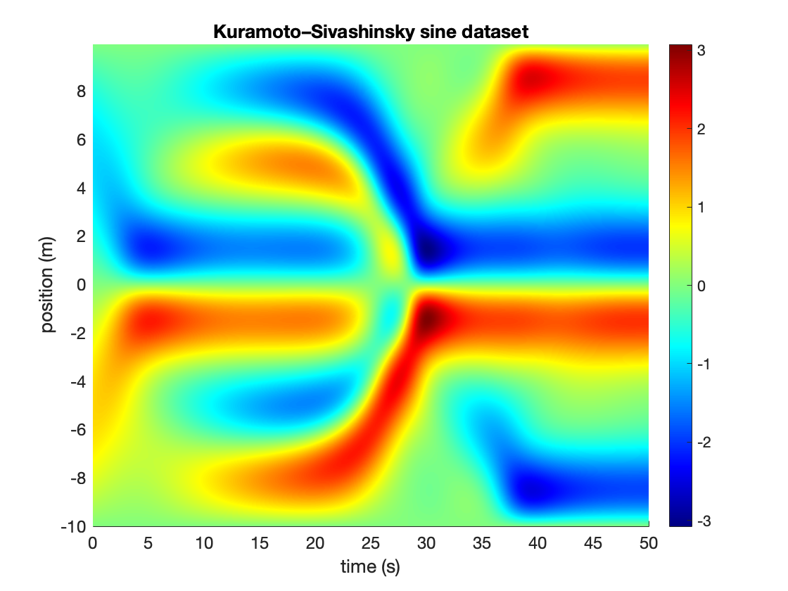
The Kuramoto–Sivashinsky (KS) equation [22] [30] is a non-linear fourth-order equation that arises in many physical contexts, including flame propagation, plasma physics, chemical physics, and combustion dynamics [25]. In one dimension, the KS equation takes the following form:
| (11) |
We test PDE-LEARN on the KS equation with , , and . For these experiments, our problem domain is . We partition into equally-sized sub-intervals and into equally-sized sub-intervals. This partition engenders a regular grid with equally-spaced grid lines along the -axis and along the -axis. We use Chebfun’s spin class to solve the KS equation on this grid subject to the initial condition
The resulting solution is our noise-free data set, which we depict in figure 6.
Using the procedure outlined at the beginning of section 5, we generate several noisy, limited data sets from the noise-free data set. We test PDE-LEARN on each data set. In each experiment, contains four layers with neurons per layer. Further, we use the same left-hand and right-hand side terms as in the previous experiments, except that we add to the RHS terms. For these experiments, we use burn-in epochs (), sparsification epochs () with , and a variable number of fine-tuning epochs (). Further, during the sparsification step, we set . Table 7 reports the results of our experiments with the KS equation.
| Noise | Identified PDE | ||||
|---|---|---|---|---|---|
Thus, PDE-LEARN can successfully identify the KS equation with up to noise. In the noise experiment, the identified PDE does not contain the term but does contain terms that are not present in the KS equation. This result is a notable departure from the results we observe with other equations, where misidentified PDEs contain too many or too few terms but never both. Even in this case, however, the identified PDE contains two of the terms of the KS equation. Thus, PDE-LEARN still recovers useful information. These results suggest that while PDE-LEARN can identify the KS equation, it appears to be less robust with this equation than with other equations we consider in this section. We discuss this result in section 6.5.
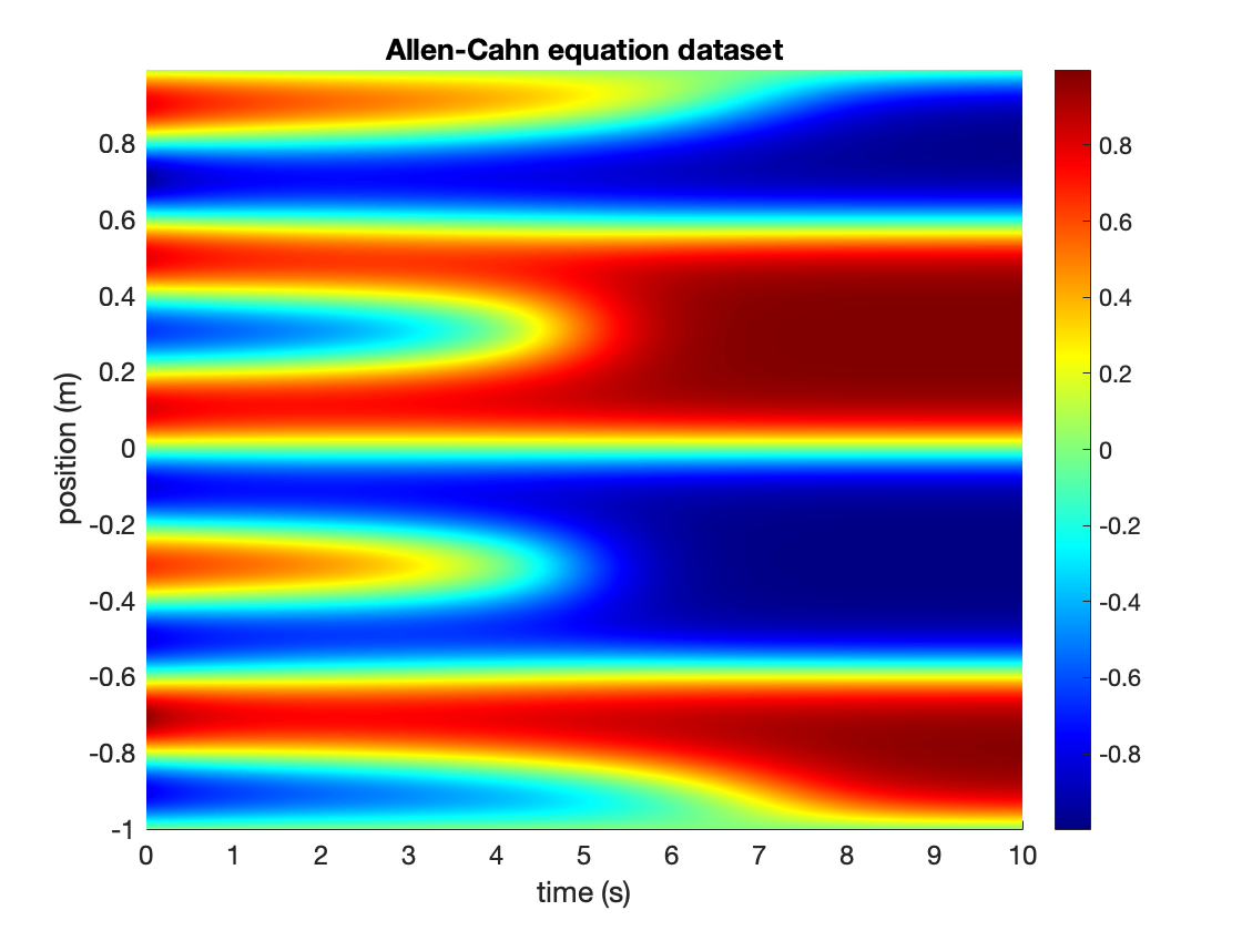
5.4 Allen-Cahn equation
Next, we consider the Allen-Cahn equation. This second-order non-linear PDE describes the separation of the constituent metals in of multi-component molten alloy mixture [2]. The Allen-Cahn equation has the following form:
| (12) |
We test PDE-LEARN on the Allen-Cahn equation with on the domain with the initial condition
The Allen-Cahn equation with this value of presents an interesting challenge for PDE-LEARN because it contains a small coefficient. As described in section 4, PDE-LEARN eliminates all components of which are smaller than a pre-defined threshold. In all our e.pngxperiments444Notably, we could rewrite PDE-LEARN to use double-precision floating point numbers, allowing for a much smaller threshold. We discuss this in section 6.3., the threshold is around . As such, the Allen-Cahn equation contains a coefficient close to the threshold. Therefore, if the identified coefficient is too far off from the true value, it risks being thresholded. Notwithstanding, PDE-LEARN performs admirably, even when the hidden PDE contains coefficients that are close to the threshold.
We partition the problem domain into a spatiotemporal grid with equally-spaced grid lines along the -axis and along the -axis. We use Chebfun’s [16] spin class to solve the Allen-Cahn equation on this grid. We refer to the resulting solutions as our noise-free Allen-Cahn data set. The script Allen_Cahn.m in the MATLAB sub-directory of our repository generates this data set. Figure 7 depicts the data sets.
For these experiments, contains five layers with neurons per layer. Further, we use the same left-hand and right-hand side terms as in the Burgers’ and KdV experiments. Table 8 reports the results of our Allen-Cahn equation experiments. In each experiment, the burn-in step lasts for epochs (), the sparsification step lasts epochs (), and the fine-tuning step lasts for epochs (). Further, during the sparsification step, we set .
| Noise | Identified PDE | ||||
|---|---|---|---|---|---|
| 1 |
-
1
For this experiment, we use during the sparsification step. If we set , PDE-LEARN identifies .
Thus, PDE-LEARN correctly identifies the Allen-Cahn equation in all but one of our experiments. Significantly, in every experiment, the right-hand side of the identified PDE contains the term with its small coefficient. These results suggest that PDE-LEARN can reliably identify small coefficients in hidden PDEs, even when they are close to the threshold. Notably, PDE-LEARN identifies the Allen-Cahn equation with up to noise and data points. Further, it correctly identifies the Allen-Cahn equation with noise using just data points. With that said, PDE-LEARN’s robustness to noise does decrease with the number of data points. In particular, it fails to identify the Allen-Cahn equation in the data points, noise experiment. In this experiment, the identified PDE is too sparse, though the two RHS terms that PDE-LEARN identifies are present in the Allen-Cahn equation.
5.5 2D Wave equation
All of the experiments we have considered thus far deal with a single spatial variable () and a Hidden PDE whose left-hand side is a time derivative. While PDEs of this form are not uncommon in physics, they do not constitute all possible PDEs of practical interest. As stated in section 4, PDE-LEARN can learn a more general class of PDEs. In this subsection, we demonstrate this ability by testing PDE-LEARN on the 2D wave equation. This second-order PDE appears in electromagnetism, structural mechanics, etc. With two spatial variables, the wave equation takes on the following form:
Here, is called the wave speed. Rearranging the above equation gives
| (13) |
where . We test PDE-LEARN on this form of the 2D wave equation with and the problem domain . We use a known solution to generate the noise-free data set. In particular,
satisfies the heat equation on the problem domain. To make our noise-free data set, we evaluate this function at points drawn from a uniform distribution over the problem domain. We then corrupt this data set using varying noise levels, engendering our noisy and limited data sets.
In all of our experiments with the wave equation, contains four layers with neurons per layer. For these experiments, we use the left-hand side term
Further, we use the following library of right-hand side terms
Table 9 reports the results of our wave equation experiments. In each experiment, the burn-in step lasts for epochs (), the sparsification step lasts epochs (), and the fine-tuning step lasts for up to epochs (). Further, during the sparsification step, we set .
| Noise | Identified PDE | ||||
|---|---|---|---|---|---|
| 1 |
-
1
For this experiment, we use during the sparsification step. If we set , PDE-LEARN identifies .
Thus, PDE-LEARN successfully identifies the wave equation in all experiments, though we did have to increase in the noise experiment. Further, in most cases, the coefficients in the identified PDE closely match those of the true PDE, deviating less than from their true values in the % and % noise experiments. However, as with other equations, these experiments reveal that PDE-LEARN does have some limitations. If we do not increase to in the % noise experiment, the identified PDE contains terms that are not present in the heat equation. However, even in this case, the identified PDE contains both RHS terms of the wave equation. Further, the coefficients of the extra terms are significantly smaller than those of the RHS terms present in the wave equation. This result adds to our observation that PDE-LEARN extracts useful information about the hidden PDE even when it fails. These experiments demonstrate that PDE-LEARN can identify PDEs with multiple spatial variables and works with arbitrary left-hand side terms.
6 Discussion
This section discusses further aspects of PDE-LEARN, with a special emphasis on our rationale behind the algorithm’s design. First, in section 6.1, we discuss hyperparameter selection with PDE-LEARN. Section 6.2 discusses why pruning (between the burn-in, sparsification, and fine-tuning steps) is necessary. In section 6.3, we discuss the loss. Section 6.4 analyzes why the coefficients in the identified PDE tend to be smaller than the corresponding coefficients in the hidden PDE. Finally, in section 6.5, we discuss some limitations of PDE-LEARN as well as potential future directions.
6.1 Hyperparameter Selection
PDE-LEARN contains many hyperparameters, including the library terms, loss function weights, , and network architecture. We did not perform hyperparameter selection in our experiments. Therefore, we do not claim our choices in the experiments are optimal; they may not be suitable in every situation.
We found that works well for the equations in our experiments. With that said, other values of may work well in other situations. is a hyperparameter and should be treated as such (with as a good default value). Our loss function weights work well in our experiments. However, we believe it may make sense to use different weights for the data and collocation losses if the data set is unusually limited or noisy. As for the library terms, our experiments suggest that PDE-LEARN can identify sparse PDEs even from a relatively large library of RHS terms. Using a large library increases the likelihood that the terms in the hidden PDE are in the library. Therefore, choosing a large library is a good default choice. Finally, for the network architecture, we believe the default choice of network architecture should contain the fewest parameters possible to learn the underlying data set (which can be empirically determined).
6.2 Pruning
Even after the sparsification step, most components of are small (a few orders of magnitude above machine epsilon) but non-zero. One likely reason for this is that PDE-LEARN works with finite precision floating-point arithmetic. Let denote machine-epsilon. If a component of , , is smaller than , then in equation 6 is smaller than machine epsilon, meaning that PDE-LEARN can not accurately compute . These results make thresholding necessary and are why we set the threshold slightly above .
The biggest drawback of pruning is that PDE-LEARN can not identify coefficients in the hidden PDE whose magnitude is smaller than the threshold. In our experiments, we use single-precision floating-point arithmetic, meaning that our threshold is around . However, PDE-LEARN can be implemented using double-precision floating-point arithmetic, allowing for a smaller threshold should the need arise.
6.3 Lp loss
As discussed in section 4, the loss effectively embeds the Iteratively Reweighted Least Squares loss into our loss function. At the start of each epoch, the loss is equal to . Crucially, however, since the weights, , in the loss are treated as constants during back-propagation, the loss is a convex function of . By contrast, the p-norm for is not convex. In particular, it contains sharp cusps along the coordinate axes. These cusps make it nearly impossible for standard optimizers (such as the Adam optimizer we use to train PDE-LEARN) to converge to a minimum of the p-norm. To illustrate this point, we tried replacing the loss with . Unsurprisingly, this change renders PDE-LEARN unusable; it fails to converge, even when training on noise-free data sets. Thus, the Iteratively Reweighted Least Squares loss function is an essential aspect of PDE-LEARN.
6.4 The coefficients in the identified PDEs are too small
In many of our experiments, the coefficients in the identified PDE are smaller than those in the hidden PDE. This effect appears to get worse as the noise level increases. We believe this is a result of how we sparsify the PDE.
During the sparsification step, the loss pushes the components of to zero. Our choice of means that the loss does a reasonable job of penalizing the number of non-zero terms, though it still pushes all components of towards zero. In principle, the collocation loss will grow if the components of deviate too much from corresponding values in the hidden PDE. Thus, the components of must balance the collocation and losses. The result is usually a compromise; the components of become as small as they can be without causing a significant increase in the collocation loss. Thus, the components of corresponding to terms in the hidden PDE generally survive the sparsification step but end up with artificially small magnitudes. This result is why we include the fine-tuning step, during which the coefficients recover and approach the corresponding values in the hidden PDE. With that said, noise makes it difficult for PDE-LEARN to precisely resolve the coefficients. This means that the collocation loss does not significantly decrease once the components of are reasonably close to the corresponding values in the hidden PDE. This result may explain why the coefficients in the identified PDE tend to shrink as the noise level increase.
Running more fine-tuning epochs generally improves the accuracy of the identified coefficients. However, if the noise is high and the data is limited, the networks can over-fit the data set. Over-fitting begins when the testing data loss increases while the training data loss decreases. In our experiments, we use an early stopping procedure to stop the fine-tuning step as soon as over-fitting begins.
6.5 Limitations and Future Directions
Our experiments in section 5 demonstrate that PDE-LEARN can learn a wide variety of PDEs. PDE-LEARN places relatively weak assumptions on the form of the underlying PDE. While the previous works discussed in section 3 assume the left-hand side of the hidden PDE is a time derivative, PDE-LEARN can learn PDEs with arbitrary left-hand side terms. With that said, the hidden PDE must be in the form of equation 1. Therefore, the user must select an appropriate library of terms. Without specialized domain knowledge, selecting an appropriate library may be challenging.
Our implementation of PDE-LEARN exclusively uses monomial library terms. However, assuming that monomial terms will work in all cases is not reasonable; thus we point out that our implementation of PDE-LEARN can be modified to work with other library terms. Even with this change, it is unclear how PDE-LEARN would perform when trying to identify PDEs whose terms are not monomials of the ’s, and their associated partial derivatives. Therefore, generalizing PDE-LEARN to use other library terms, and exploring how this impacts PDE-LEARN’s performance, represents a potential future area of research.
Finally, it is worth noting that PDE-LEARN’s performance varies by equation. PDE-LEARN had little trouble discovering the Brugers’, KdV, Allen-Cahn, and Heat equations. However, PDE-LEARN only identify the KS equation with noise. It is not immediately clear why this equation is more challenging for PDE-LEARN to identify, though past works have reported similar results [15]. Identifying factors (both in the hidden PDE and the data set) that impact PDE-LEARN’s performance represents an important area of future research.
7 Conclusion
This paper introduced PDE-LEARN, a novel PDE-discovery algorithm to identify human-readable PDEs from noisy and limited data. PDE-LEARN utilizes Rational Neural Networks, targeted collocation points, and a three-part loss function inspired by Iteratively Reweighted Least Squares. Further, unlike many previous works, PDE-LEARN can identify PDEs with multiple spatial variables and arbitrary left-hand side terms (see equation 1). The general form of the hidden PDE, equation 1, gives PDE-LEARN tremendous flexibility in discovering PDEs from data. Our experiments in section 5 demonstrate that PDE-LEARN can identify a variety of PDEs from noisy, limited data sets.
PDE-LEARN appears to be an effective tool for PDE discovery. Its ability to identify a variety of linear and non-linear PDEs, including those with multiple spatial variables, suggests that PDE-LEARN may be useful in discovering governing equations for physical systems that, until now, have evaded such descriptions.
8 Acknowledgements
This work is supported by the Office of Naval Research (ONR), under grant N00014-22-1-2055. Further, Robert Stephany is supported his NDSEG fellowship.
References
- [1] Clare I Abreu, Jonathan Friedman, Vilhelm L Andersen Woltz and Jeff Gore “Mortality causes universal changes in microbial community composition” In Nature communications 10.1 Nature Publishing Group, 2019, pp. 1–9
- [2] Samuel M Allen and John W Cahn “A microscopic theory for antiphase boundary motion and its application to antiphase domain coarsening” In Acta metallurgica 27.6 Elsevier, 1979, pp. 1085–1095
- [3] Daniel R Amor, Christoph Ratzke and Jeff Gore “Transient invaders can induce shifts between alternative stable states of microbial communities” In Science advances 6.8 American Association for the Advancement of Science, 2020, pp. eaay8676
- [4] Steven Atkinson et al. “Data-driven discovery of free-form governing differential equations” In arXiv preprint arXiv:1910.05117, 2019
- [5] Cea Basdevant et al. “Spectral and finite difference solutions of the Burgers equation” In Computers & fluids 14.1 Elsevier, 1986, pp. 23–41
- [6] Harry Bateman “Some recent researches on the motion of fluids” In Monthly Weather Review 43.4, 1915, pp. 163–170
- [7] Atilim Gunes Baydin, Barak A Pearlmutter, Alexey Andreyevich Radul and Jeffrey Mark Siskind “Automatic differentiation in machine learning: a survey” In Journal of machine learning research 18 Journal of Machine Learning Research, 2018
- [8] Jens Berg and Kaj Nyström “Neural network augmented inverse problems for PDEs” In arXiv preprint arXiv:1712.09685, 2017
- [9] Josh Bongard and Hod Lipson “Automated reverse engineering of nonlinear dynamical systems” In Proceedings of the National Academy of Sciences 104.24 National Acad Sciences, 2007, pp. 9943–9948
- [10] Christophe Bonneville and Christopher J Earls “Bayesian Deep Learning for Partial Differential Equation Parameter Discovery with Sparse and Noisy Data” In arXiv preprint arXiv:2108.04085, 2021
- [11] Gert-Jan Both, Subham Choudhury, Pierre Sens and Remy Kusters “DeepMoD: Deep learning for Model Discovery in noisy data” In Journal of Computational Physics 428 Elsevier, 2021, pp. 109985
- [12] Nicolas Boullé, Yuji Nakatsukasa and Alex Townsend “Rational neural networks” In Advances in Neural Information Processing Systems 33, 2020, pp. 14243–14253
- [13] Steven L Brunton, Joshua L Proctor and J Nathan Kutz “Discovering governing equations from data by sparse identification of nonlinear dynamical systems” In Proceedings of the national academy of sciences 113.15 National Acad Sciences, 2016, pp. 3932–3937
- [14] Rick Chartrand and Wotao Yin “Iteratively reweighted algorithms for compressive sensing” In 2008 IEEE international conference on acoustics, speech and signal processing, 2008, pp. 3869–3872 IEEE
- [15] Zhao Chen, Yang Liu and Hao Sun “Physics-informed learning of governing equations from scarce data” In Nature communications 12.1 Nature Publishing Group, 2021, pp. 1–13
- [16] Tobin A Driscoll, Nicholas Hale and Lloyd N Trefethen “Chebfun guide” Pafnuty Publications, Oxford, 2014
- [17] Xavier Glorot and Yoshua Bengio “Understanding the difficulty of training deep feedforward neural networks” In Proceedings of the thirteenth international conference on artificial intelligence and statistics, 2010, pp. 249–256 JMLR WorkshopConference Proceedings
- [18] Daniel R Gurevich, Patrick AK Reinbold and Roman O Grigoriev “Robust and optimal sparse regression for nonlinear PDE models” In Chaos: An Interdisciplinary Journal of Nonlinear Science 29.10 AIP Publishing LLC, 2019, pp. 103113
- [19] Isabelle Guyon, Jason Weston, Stephen Barnhill and Vladimir Vapnik “Gene selection for cancer classification using support vector machines” In Machine learning 46.1 Springer, 2002, pp. 389–422
- [20] Diederik P Kingma and Jimmy Ba “Adam: A method for stochastic optimization” In arXiv preprint arXiv:1412.6980, 2014
- [21] Diederik Johannes Korteweg and Gustav De Vries “XLI. On the change of form of long waves advancing in a rectangular canal, and on a new type of long stationary waves” In The London, Edinburgh, and Dublin Philosophical Magazine and Journal of Science 39.240 Taylor & Francis, 1895, pp. 422–443
- [22] Yoshiki Kuramoto and Toshio Tsuzuki “Persistent propagation of concentration waves in dissipative media far from thermal equilibrium” In Progress of theoretical physics 55.2 Oxford University Press, 1976, pp. 356–369
- [23] Dong C Liu and Jorge Nocedal “On the limited memory BFGS method for large scale optimization” In Mathematical programming 45.1 Springer, 1989, pp. 503–528
- [24] Daniel A Messenger and David M Bortz “Weak SINDy for partial differential equations” In Journal of Computational Physics 443 Elsevier, 2021, pp. 110525
- [25] Demetrios T Papageorgiou and Yiorgos S Smyrlis “The route to chaos for the Kuramoto-Sivashinsky equation” In Theoretical and Computational Fluid Dynamics 3.1 Springer, 1991, pp. 15–42
- [26] Maziar Raissi “Deep hidden physics models: Deep learning of nonlinear partial differential equations” In The Journal of Machine Learning Research 19.1 JMLR. org, 2018, pp. 932–955
- [27] Samuel H Rudy, Steven L Brunton, Joshua L Proctor and J Nathan Kutz “Data-driven discovery of partial differential equations” In Science Advances 3.4 American Association for the Advancement of Science, 2017, pp. e1602614
- [28] Hayden Schaeffer “Learning partial differential equations via data discovery and sparse optimization” In Proceedings of the Royal Society A: Mathematical, Physical and Engineering Sciences 473.2197 The Royal Society Publishing, 2017, pp. 20160446
- [29] Michael Schmidt and Hod Lipson “Distilling free-form natural laws from experimental data” In science 324.5923 American Association for the Advancement of Science, 2009, pp. 81–85
- [30] Gregory I Sivashinsky “Nonlinear analysis of hydrodynamic instability in laminar flames—I. Derivation of basic equations” In Acta astronautica 4.11, 1977, pp. 1177–1206
- [31] Robert Stephany and Christopher Earls “PDE-READ: Human-readable partial differential equation discovery using deep learning” In Neural Networks 154 Elsevier, 2022, pp. 360–382